Other Topics
The last chapter of the book is a tour: ten topics in sixteen pages, most stated in a paragraph with a pointer to the literature. These notes keep the book's order and fill in what a reader needs to work with each topic: why measurement error attenuates a slope and how SIMEX and deconvolution undo it (and why deconvolution with Normal errors converges only at a logarithmic rate), why inverse problems are ill-posed, how the Dirichlet process works, how to estimate the parametric part of a partially linear model at the \(\sqrt n\) rate, why cross-validation fails under correlation, why classification is easier than regression, how sieves trade bias for variance, why isotonic regression needs no bandwidth and converges at \(n^{-1/3}\), and where the \(n^{1/4}\) detection boundary of nonparametric testing comes from.
Ch. 1 Introduction Ch. 2 The cdf and functionals Ch. 3 Bootstrap and jackknife Ch. 4 Smoothing Ch. 5 Regression Ch. 6 Density estimation Ch. 7 Normal means and minimax Ch. 8 Orthogonal functions Ch. 9 Wavelets Ch. 10 Other topics
How to read these notes
They follow the book. Sections carry the book's numbers (10.1, 10.2, ...) and every displayed equation that appears in the book carries the book's own equation number, e.g. \((10.5)\). Equations without a number are steps that the book skips.
Filling the gaps. The chapter states almost everything without proof. A Filling the gap box gives the argument for each claim: complete proofs where the result is elementary or central, and a precise statement with a proof sketch and a reference where a full proof would take a paper (the lower bound for deconvolution, the limit law of isotonic regression). Proofs start hidden: open one with its bar, or use the button below.
Figures and demonstrations. The book has two figures. Figure 10.1 is a diagram (three nodes and two arrows) and is not reproduced; Figure 10.2 is a sketch of SIMEX and is computed here from simulated data. Because the chapter is a survey, eleven supplementary figures (10.S1 to 10.S11) illustrate the topics and solve the computational exercises. All are made by the Python code. The ▶ Demo boxes open an interactive demonstration already set to the case being discussed.
Main reference
L. Wasserman, All of Nonparametric Statistics, Springer (2006), Chapter 10, pages 227–242 (book website: www.stat.cmu.edu/~larry/all-of-nonpar). Section, equation, figure and exercise numbers below refer to this book. Further reading is listed in the references.
The explanations, derivations, figures and code are my own; equations are cited by their numbers in the book.
Companion courses
Each topic of this chapter touches material elsewhere in this course and in the companion courses on this site:
- This course: linear smoothers and cross-validation (Sections 5.2 and 5.3), local polynomial bias (5.4), kernels (4.2), kernel density estimation (Chapter 6), the Normal means model, Sobolev ellipsoids and minimax rates (Chapter 7), orthogonal series (Chapter 8) and adaptive methods (Chapter 9).
- Probability and Statistical Inference (Wasserman 2004, same author and notation): least squares (Section 13.1), Bayesian inference (11.2, large-sample behaviour in 11.5), tests and their power (10.6), the Bayes classifier (22.2), kernel density estimation (20.3).
- Statistical Learning: Theory and Methods: logistic regression (Section 4.4), statistical decision theory for classification (2.4), cross-validation (7.10), additive and partially linear models (9.1).
- Bayesian and Probabilistic Machine Learning: Gaussian processes, the most common nonparametric prior for regression functions (Section 6.4); kernel density estimators (2.5). (The site has no Dirichlet process material yet; Filling the gap 10.9 develops it here.)
New here: the SIMEX limit curve and why the rational extrapolant is exact, the excess bias (10.3) via Tweedie's formula, the full second-order correction (10.14), the exact risk of the deconvolution estimator and its logarithmic rate, Backus–Gilbert kernels, the Dirichlet process posterior, the double-residual estimator, the bias of cross-validation under correlation, the plug-in classification bound, isotonic regression from first principles, and Ingster's \(n^{1/4}\) boundary with both bounds proved.
The chapter at a glance
- 10.1 Errors in \(X\) attenuate the slope by \(\lambda=\sigma_x^2/(\sigma_x^2+\sigma_u^2)\); method of moments and SIMEX correct it (Figure 10.2); deconvolution estimates the density of \(X\) by dividing characteristic functions, at the price of a slow rate.
- 10.2 Blurred regression \(Y_i=\int K_ir+\epsilon_i\): the Backus–Gilbert kernel, ill-posedness and Tikhonov regularisation.
- 10.3 Nonparametric Bayes: the Dirichlet process (Filling the gap 10.9) and, in Exercise 10.7, Gaussian priors in the Normal means model.
- 10.4 The partially linear model (10.29): \(\beta\) at rate \(\sqrt n\) by double residuals.
- 10.5–10.7 Correlated errors break leave-one-out cross-validation; plug-in classification; sieves.
- 10.8 Isotonic regression: convex minorant, pool-adjacent-violators, the \(n^{-1/3}\) rate (10.30).
- 10.9–10.10 Ingster's critical radius \(R_n^*\); testing qualitative hypotheses; binning for fast computation.
Notation. \(\Xb=X+U\) is the error-prone covariate (the demos call it \(W\)); \(\psi\), \(\psi^\bullet\), \(\psi_U\) are the characteristic functions of \(X\), \(\Xb\), \(U\) (\(\psi(t)=\E e^{itX}\)) and \(\psi_K(t)=\int e^{itx}K(x)\,\d x\); \(\phi_\sigma\) is the \(N(0,\sigma^2)\) density.
Prerequisites. Linear smoothers and cross-validation (Chapter 5), kernel density estimation, characteristic functions and Parseval's identity, conjugate Bayesian updating.
10.1 Measurement Error
pp. 227–233 In the errors-in-variables model we want the regression of \(Y\) on \(X\), but observe \(\Xb\) instead of \(X\):
\[ Y_i=r(X_i)+\epsilon_i,\qquad \Xb_i=X_i+U_i,\qquad \E(U_i)=0. \]Throughout, \(U\) is independent of \((X,\epsilon)\) and its distribution is known (from replicate measurements or from knowledge of the instrument). Figure 10.1 of the book draws this as a graph \(X\to Y\), \(X\to\Xb\) with \(X\) unobserved; it is a diagram and is not reproduced. Regressing \(Y\) on \(\Xb\) estimates \(m(w)=\E(Y\given\Xb=w)=\E(r(X)\given\Xb=w)\), which is not \(r\).
The linear case: attenuation
For \(Y=\beta_0+\beta_1X+\epsilon\) with \(\V(X)=\sigma_x^2\), \(\V(U)=\sigma_u^2\), the least squares slope \(\hb_1\) of \(Y\) on \(\Xb\) satisfies
\[ \hb_1\xrightarrow{\text{a.s.}}\lambda\beta_1, \tag{10.1} \] \[ \lambda=\frac{\sigma_x^2}{\sigma_x^2+\sigma_u^2}\lt1. \tag{10.2} \]Filling the gap 10.1: proof of (10.1) (Exercise 10.2) p. 228
Proof
Assume \((X_i,\epsilon_i,U_i)\) iid with finite second moments, \(\epsilon\) and \(U\) mean zero, \(U\) independent of \((X,\epsilon)\) and \(\epsilon\) uncorrelated with \(X\). The slope is a ratio of sample moments, \(\hb_1=S_{\bullet Y}/S_{\bullet\bullet}\) with \(S_{\bullet Y}=n^{-1}\sum(\Xb_i-\bar X^\bullet)(Y_i-\bar Y)\) and \(S_{\bullet\bullet}=n^{-1}\sum(\Xb_i-\bar X^\bullet)^2\). By the strong law of large numbers applied to \(\Xb_iY_i\), \(\Xb_i\), \(Y_i\) and \((\Xb_i)^2\),
\[ S_{\bullet Y}\to\cov(X+U,\beta_0+\beta_1X+\epsilon)=\beta_1\sigma_x^2,\qquad S_{\bullet\bullet}\to\V(X+U)=\sigma_x^2+\sigma_u^2 \]almost surely: the cross covariances \(\cov(U,X)\), \(\cov(U,\epsilon)\), \(\cov(X,\epsilon)\) vanish. The map \((a,b)\mapsto a/b\) is continuous at \(b=\sigma_x^2+\sigma_u^2\gt0\), so \(\hb_1\to\beta_1\sigma_x^2/(\sigma_x^2+\sigma_u^2)=\lambda\beta_1\) almost surely. ∎
The same argument shows that the intercept is biased too: \(\hb_0\to\beta_0+(1-\lambda)\beta_1\E X\). The noise in the covariate behaves like a regression towards the mean of \(X\): a large observed \(\Xb\) is, on average, partly a large \(U\).
With \(\sigma_u^2\) known and \(\sigma_\bullet^2=\sigma_x^2+\sigma_u^2\), estimate \(\sigma_x^2\) by \(\hat\sigma_x^2=\hat\sigma_\bullet^2-\sigma_u^2\) (10.4), then \(\hat\lambda=(\hat\sigma_\bullet^2-\sigma_u^2)/\hat\sigma_\bullet^2\) and
\[ \tb_1=\frac{\hb_1}{\hat\lambda}=\frac{\hat\sigma_\bullet^2}{\hat\sigma_\bullet^2-\sigma_u^2}\,\hb_1, \tag{10.5} \]the method of moments estimator. SIMEX (simulation extrapolation; Cook and Stefanski 1994) instead adds more error on purpose: with \(Z_i\sim N(0,1)\) independent of the data, regress \(Y\) on \(\widetilde X_i=\Xb_i+\sqrt\rho\,\sigma_uZ_i\). The slope then estimates
\[ \Omega(\rho)=\frac{\beta_1\sigma_x^2}{\sigma_x^2+(1+\rho)\sigma_u^2}. \tag{10.6} \]Average the slopes over \(B\) independent draws to get \(\widehat\Omega(\rho)\) at \(\rho=0,0.25,\dots,2\), fit a curve, and evaluate it at \(\rho=-1\), where \(\Omega(-1)=\beta_1\). The book suggests the rational curve
\[ G(\rho;\gamma_1,\gamma_2,\gamma_3)=\gamma_1+\frac{\gamma_2}{\gamma_3+\rho}, \tag{10.7} \] \[ \tb_1=G(-1;\hat\gamma_1,\hat\gamma_2,\hat\gamma_3), \tag{10.8} \]or, more simply, a quadratic \(Q(\rho)=\gamma_1+\gamma_2\rho+\gamma_3\rho^2\) with \(\tb_1=\hat\gamma_1-\hat\gamma_2+\hat\gamma_3\).
Filling the gap 10.2: why SIMEX works, and when the quadratic is not enough pp. 229–230
Derivation
(10.5). \(\hat\sigma_\bullet^2\to\sigma_x^2+\sigma_u^2\) almost surely, so \(\hat\lambda\to\lambda\) and \(\tb_1=\hb_1/\hat\lambda\to\lambda\beta_1/\lambda=\beta_1\) by (10.1) and continuity. The estimator is unstable when \(\hat\sigma^2_\bullet\) is close to \(\sigma_u^2\) (a small reliability ratio): \(\hat\lambda\) can then be near zero or negative.
(10.6). Given the data, \(\widetilde X_i=X_i+(U_i+\sqrt\rho\,\sigma_uZ_i)\), and the combined error \(U_i+\sqrt\rho\,\sigma_uZ_i\) has mean zero, variance \((1+\rho)\sigma_u^2\) and is independent of \((X_i,\epsilon_i)\). Applying (10.1)–(10.2) with \(\sigma_u^2\) replaced by \((1+\rho)\sigma_u^2\) gives the limit (10.6). The scaling by \(\sigma_u\) matters: the book's text adds \(\sqrt\rho\,Z_i\) without it, which would give the limit \(\beta_1\sigma_x^2/(\sigma_x^2+\sigma_u^2+\rho)\) and a wrong extrapolation point (see the notes on the book). Averaging over \(b=1,\dots,B\) removes the simulation noise, not any bias.
The rational extrapolant is exact. Divide numerator and denominator of (10.6) by \(\sigma_u^2\):
\[ \Omega(\rho)=\frac{\beta_1\sigma_x^2/\sigma_u^2}{(1+\sigma_x^2/\sigma_u^2)+\rho}=G(\rho;\,0,\ \beta_1\sigma_x^2/\sigma_u^2,\ 1+\sigma_x^2/\sigma_u^2). \]So the curve (10.7) contains the true limit curve, with \(\gamma_3=1+\sigma_x^2/\sigma_u^2\gt1\) (the pole lies to the left of \(-1\)), and \(G(-1)=\gamma_2/(\gamma_3-1)=\beta_1\). Fitted to the exact \(\Omega\), the rational extrapolant returns \(\beta_1\) to machine precision, and as \(n\to\infty\) the fitted \(\hat\gamma\) converge to these values.
The quadratic leaves a bias. A polynomial fitted on \([0,2]\) cannot follow the pole at \(-\gamma_3\) when \(\gamma_3\) is close to 1 (large measurement error). With the grid \(\rho=0,0.25,\dots,2\), the least squares quadratic fitted to the exact \(\Omega\) gives \(Q(-1)=0.899\,\beta_1\) when \(\sigma_u^2/\sigma_x^2=0.49\) (the case of Figure 10.2), and \(0.688\,\beta_1\) when \(\sigma_u^2/\sigma_x^2=1.21\). It is still much better than the naive \(\lambda\beta_1\) (0.671 and 0.452). SIMEX with a quadratic is therefore approximately consistent; its appeal is that it needs nothing beyond the ability to refit the estimator, so it applies unchanged to nonlinear and nonparametric estimators. ∎
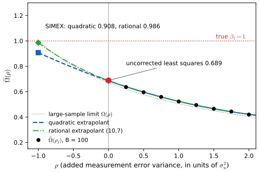
fig_10_2. Reproduces Wasserman (2006), Figure 10.2. Download: PDF · SVGSee also (companion course): Probability and Statistical Inference, Section 13.1 (simple linear regression).
The nonparametric case
Staudenmayer and Ruppert (2004): if a local polynomial of odd degree is fitted to \((\Xb_i,Y_i)\), its asymptotic bias exceeds the usual one by
\[ \sigma_u^2\left(\frac{f'(x)}{f(x)}\,r'(x)+\frac{r''(x)}{2}\right), \tag{10.3} \]with \(f\) the density of \(X\). The derivation below shows where both terms come from.
Filling the gap 10.3: the excess bias (10.3) from Tweedie's formula p. 228
Derivation
Take \(U\sim N(0,\sigma^2)\) independent of \(X\), and let \(f_\bullet=f*\phi_\sigma\) be the density of \(\Xb\). The naive smoother estimates \(m(w)=\E(r(X)\given\Xb=w)\) with the usual (error-free) bias, so the excess bias is \(m(w)-r(w)\). Two exact identities hold for Normal errors (Tweedie's formulas). Differentiating \(f_\bullet(w)=\int f(x)\phi_\sigma(w-x)\,\d x\) under the integral, with \(\phi_\sigma'(u)=-(u/\sigma^2)\phi_\sigma(u)\) and \(\phi_\sigma''(u)=(u^2/\sigma^4-1/\sigma^2)\phi_\sigma(u)\),
\[ \E(X-w\given\Xb=w)=\sigma^2\frac{f_\bullet'(w)}{f_\bullet(w)},\qquad \E\big((X-w)^2\given\Xb=w\big)=\sigma^2+\sigma^4\frac{f_\bullet''(w)}{f_\bullet(w)}. \](For the first: \(f_\bullet'(w)=-\sigma^{-2}\int(w-x)f(x)\phi_\sigma(w-x)\,\d x=-\sigma^{-2}f_\bullet(w)\E(w-X\given\Xb=w)\); the second is the same computation with \(\phi''_\sigma\).) Now expand \(r\) around \(w\) with a remainder, assuming \(r'''\) bounded:
\[ m(w)=r(w)+r'(w)\,\E(X-w\given\Xb=w)+\tfrac12r''(w)\,\E\big((X-w)^2\given\Xb=w\big)+O\big(\E(|X-w|^3\given\Xb=w)\big). \]The conditional third absolute moment is \(O(\sigma^3)\) when \(f\) is bounded away from zero near \(w\), and \(f_\bullet'/f_\bullet=f'/f+O(\sigma^2)\) when \(f\) has three bounded derivatives. Substituting,
\[ m(w)-r(w)=\sigma^2\Big(\frac{f'(w)}{f(w)}r'(w)+\frac{r''(w)}{2}\Big)+O(\sigma^3), \]which is (10.3). The first term is a shift: the true \(X\) behind an observed \(\Xb=w\) tends to lie towards the denser side. The second is a smearing: \(r\) is averaged over a window of width \(\sigma\), which flattens peaks (\(r''\lt0\)) and fills valleys. Panel (c) of Figure 10.S1 compares the exact \(m-r\) with \(\sigma^2r''/2\) for the function of Exercise 10.5 (uniform \(X\), so \(f'=0\) inside the support): the approximation is good at \(\sigma_u=0.05\) and overshoots the dip at \(\sigma_u=0.1\), where \(\sigma_u\) is no longer small against the width 0.18 of the peak. ∎
Besides SIMEX, which applies pointwise to \(\hr_n(x,\rho)\), the book describes the Fan and Truong (1993) kernel estimator
\[ \hr_n(x)=\frac{\sum_{i=1}^nK_n\big(\frac{x-\Xb_i}{h_n}\big)Y_i}{\sum_{i=1}^nK_n\big(\frac{x-\Xb_i}{h_n}\big)},\qquad K_n(x)=\frac{1}{2\pi}\int e^{-itx}\frac{\phi_K(t)}{\phi_U(t/h_n)}\,\d t, \tag{10.9} \]whose kernel is the deconvolving kernel of (10.21) below, and Stefanski's "small \(\sigma_u\)" correction. Write the naive estimator as \(\hr_n(x)=\sum_iY_i\ell_i(x,\Xb_i)\) (10.10), and \(r_n^*(x)=\sum_iY_i\ell_i(x,X_i)\) for the infeasible estimator using the true covariates. Expanding in \(U_i=\Xb_i-X_i\) gives (10.11), the excess bias (10.12) and its estimate (10.13), and the corrected estimator
\[ \widetilde r_n(x)=\hr_n(x)-\hat b(x)=\hr_n(x)-\frac{\sigma_u^2}{2}\sum_{i=1}^n\hr_n(\Xb_i)\,\ell''(x,\Xb_i). \tag{10.14} \]Filling the gap 10.4: the second-order correction, done carefully p. 231, (10.11)–(10.14)
Derivation
For a kernel smoother the weight \(\ell_i\) depends on all covariates, not on \(X_i\) alone: for Nadaraya–Watson, \(\ell_i=K_i/D\) with \(K_i=K((x-X_i)/h)\) and \(D=\sum_jK_j\). Treat \(\hr_n(x)\) as a function of the vector \((X_1,\dots,X_n)\) and expand to second order in the errors \(U_i\):
\[ \hr_n(x)=r_n^*(x)+\sum_iU_i\,\partial_i r_n^*(x)+\frac12\sum_{i,k}U_iU_k\,\partial_i\partial_kr_n^*(x)+\dots \]Conditionally on \((X,Y)\) the \(U_i\) are independent with mean 0 and variance \(\sigma_u^2\): the linear term has mean zero, and only the diagonal \(i=k\) survives in the quadratic term. Averaging also over \(\epsilon\) (which replaces \(Y_j\) by \(r(X_j)\)), the excess bias is
\[ b(x)=\frac{\sigma_u^2}{2}\sum_{i=1}^n\frac{\partial^2r_n^*(x)}{\partial X_i^2}. \]For Nadaraya–Watson, with \(a_i=\partial K_i/\partial X_i\) and \(c_i=\partial^2K_i/\partial X_i^2\), the quotient rule gives the closed form
\[ \sum_i\frac{\partial^2r_n^*}{\partial X_i^2}=\sum_i\big(Y_i-r_n^*(x)\big)\Big(\frac{c_i}{D}-\frac{2a_i^2}{D^2}\Big), \]which I confirmed against finite differences. Estimating it at the observed \(\Xb_i\), with \(Y_i\) replaced by a pilot fit \(\hr_n(\Xb_i)\), gives the correction used in the code. The factor \(Y_i-r_n^*(x)\) is the important difference from (10.12)–(10.13) read literally (only the numerator weight differentiated): the correct correction vanishes when \(r\) is constant, as it must since every smoother reproduces constants, while the literal one does not (it is not invariant to adding a constant to \(Y\)). Exercise 10.5 and Figure 10.S1 show the corrected estimator removing about 40% of the integrated squared error of the naive one. ∎
Deconvolution
Now \(X_1,\dots,X_n\sim F\) are unobserved and \(\Xb_i=X_i+U_i\). The density of \(\Xb\) is the convolution
\[ f^\bullet(x)=\int f(s)f_U(x-s)\,\d s, \tag{10.15} \]so \(\psi^\bullet(t)=\psi(t)\psi_U(t)\) and
\[ \psi(t)=\frac{\psi^\bullet(t)}{\psi_U(t)}. \tag{10.16} \]An estimate \(\hf^\bullet\) gives \(\widehat\psi^\bullet(t)=\int e^{itx}\hf^\bullet(x)\,\d x\) (10.17); Fourier inversion \(f(x)=(2\pi)^{-1}\int e^{-itx}\psi(t)\,\d t\) (10.18) suggests
\[ \hf(x)=\frac1{2\pi}\int e^{-itx}\frac{\widehat\psi^\bullet(t)}{\psi_U(t)}\,\d t. \tag{10.19} \]When \(\hf^\bullet\) is a kernel estimator this becomes a kernel estimator with a special kernel:
\[ \hf(x)=\frac1{nh}\sum_{j=1}^nK^*\Big(\frac{x-\Xb_j}{h},h\Big), \tag{10.20} \] \[ K^*(t,h)=\frac1{2\pi}\int e^{-itu}\frac{\psi_K(u)}{\psi_U(u/h)}\,\d u. \tag{10.21} \]Filling the gap 10.5: proof of (10.16) and (10.20) (Exercise 10.3) p. 232
Proof
(10.16). By independence, \(\psi^\bullet(t)=\E e^{it(X+U)}=\E e^{itX}\E e^{itU}=\psi(t)\psi_U(t)\). Division requires \(\psi_U(t)\ne0\) for all \(t\); this holds for Normal, Laplace and Cauchy errors, and it is the condition for \(f\) to be identified (if \(\psi_U\) vanished on an interval, two densities differing only at those frequencies would give the same \(f^\bullet\)).
(10.20). Assume \(\psi_K\) vanishes outside \([-1,1]\) (so all integrals below are over a bounded set) and \(\psi_U\) has no zeros. The kernel estimate \(\hf^\bullet(x)=(nh)^{-1}\sum_jK((x-\Xb_j)/h)\) has Fourier transform
\[ \widehat\psi^\bullet(t)=\frac1n\sum_{j=1}^n\int e^{itx}\frac1hK\Big(\frac{x-\Xb_j}{h}\Big)\d x=\frac1n\sum_{j=1}^ne^{it\Xb_j}\psi_K(th) \](substitute \(x=\Xb_j+hv\)). Insert this in (10.19) and exchange the finite sum and the integral:
\[ \hf(x)=\frac1n\sum_{j=1}^n\frac1{2\pi}\int e^{-it(x-\Xb_j)}\frac{\psi_K(th)}{\psi_U(t)}\d t=\frac1{nh}\sum_{j=1}^n\frac1{2\pi}\int e^{-iu(x-\Xb_j)/h}\frac{\psi_K(u)}{\psi_U(u/h)}\d u, \]after the substitution \(u=th\). The inner integral is \(K^*((x-\Xb_j)/h,h)\). ∎
Remarks. (i) The book writes \(e^{+itu}\) in (10.21); for a symmetric kernel and a symmetric error both \(\psi_K\) and \(\psi_U\) are real and even, and the two signs give the same real kernel. (ii) \(\int K^*(t,h)\,\d t=\psi_K(0)/\psi_U(0)=1\), but \(K^*\) takes negative values, so \(\hf\) can be negative. (iii) The kernel used throughout these notes has \(\psi_K(s)=(1-s^2)^3\) on \([-1,1]\); I checked numerically that the two forms of the estimator agree to \(10^{-16}\). (iv) The regression kernel \(K_n\) of (10.9) is the same \(K^*\): numerator and denominator of (10.9) are deconvolution estimates of \(\int r f\) and \(f\) near \(x\).
The risk is
\[ \E(\hf(y)-f(y))^2\approx ch^4+\frac1{2\pi nh}\int\Big(\frac{\psi_K(t)}{|\psi_U(t/h)|}\Big)^2\d t, \tag{10.22} \] \[ c=\frac14\Big(\int y^2K(y)\,\d y\Big)^2\int(f''(y))^2\,\d y \tag{10.23} \](integrated over \(y\); the book prints the first integral of (10.23) without the square, see the notes on the book). Because \(\psi_U(t/h)\) sits in the denominator, a smooth error density (fast-decaying \(\psi_U\)) makes the variance explode: for Normal errors the best rate is \(O((\log n)^{-2})\), and the best bandwidth is about \(\sigma_u/\sqrt{\log n}\) (Stefanski 1990).
Filling the gap 10.6: the exact risk, (10.22)–(10.23), and the logarithmic rate p. 233
Derivation
Exact MISE. Write the estimator through its Fourier transform, \(\widehat\psi(t)=\widehat\psi_{\rm emp}(t)\psi_K(th)m(t)\) with \(\widehat\psi_{\rm emp}(t)=n^{-1}\sum_je^{it\Xb_j}\) and \(m=1/\psi_U\) (the same formula with \(m=1\) is the naive kernel estimator). Since \(\E\widehat\psi_{\rm emp}=\psi^\bullet\) and \(\E|\widehat\psi_{\rm emp}(t)-\psi^\bullet(t)|^2=(1-|\psi^\bullet(t)|^2)/n\), Parseval's identity \(\int|g|^2=(2\pi)^{-1}\int|\widehat g|^2\) gives
\[ \mise(h)=\frac1{2\pi}\int\Big\{\big|\psi_K(th)m(t)\psi_U(t)-1\big|^2|\psi(t)|^2+\frac{\psi_K(th)^2|m(t)|^2\big(1-|\psi(t)\psi_U(t)|^2\big)}n\Big\}\d t. \]This is exact, for every \(n\) and \(h\); a simulation with 300 samples agreed with it within its standard error. The code and the demo use it for all risk curves.
(10.22)–(10.23). With \(m=1/\psi_U\) the first term is \((2\pi)^{-1}\int|\psi_K(th)-1|^2|\psi|^2\): exactly the integrated squared bias of an ordinary kernel estimator built from the unobserved \(X_i\). Indeed \(\E\hf(x)=(K_h*f)(x)\): deconvolution removes the measurement error bias completely. The usual Taylor argument (Chapter 6) gives \(\int(K_h*f-f)^2=\tfrac14h^4\sigma_K^4\int(f'')^2+o(h^4)\) with \(\sigma_K^2=\int y^2K\); this is (10.23) with the square. For \(\psi_K(s)=(1-s^2)^3\), \(\sigma_K^2=-\psi_K''(0)=6\), and the exact bias term divided by \(h^4\) is 1.88 at \(h=0.05\) for \(f=\phi\), against \(\frac14\cdot36\cdot\frac{3}{8\sqrt\pi}=1.90\) (with the unsquared moment it would be 0.32). The variance term, after substituting \(t=s/h\), is \((2\pi nh)^{-1}\int\psi_K(s)^2|\psi_U(s/h)|^{-2}\d s\) minus the \(O(1/n)\) part \(\int|\psi\psi_K|^2/(2\pi n)\): this is (10.22).
The Normal-error rate. For \(\psi_U(t)=e^{-\sigma^2t^2/2}\) the variance is \((2\pi nh)^{-1}\int_{-1}^1(1-s^2)^6e^{\sigma^2s^2/h^2}\d s\). Put \(a=\sigma^2/h^2\). Near \(s=1\), with \(s=1-v\), \((1-s^2)^6\le(2v)^6\) and \(e^{as^2}\le e^{a}e^{-2a v+av^2}\le e^ae^{-av}\) for \(v\le1\), so the integral is at most \(2e^a\int_0^\infty64v^6e^{-av}\d v=2\cdot64\cdot720\,e^aa^{-7}\). Choose \(h=\sigma/\sqrt{\log n}\), i.e. \(e^a=n\): the variance is \(O(h^{-1}(\log n)^{-7})=O((\log n)^{-6.5})\), negligible next to the bias \(ch^4=c\sigma^4(\log n)^{-2}\). Hence \(\mise=O((\log n)^{-2})\). A smaller \(h\) (with \(e^{a}\) a larger power of \(n\)) makes the variance grow polynomially, so \(h\) cannot shrink faster than \(\sigma/\sqrt{\log n}\) to first order, and this choice is asymptotically right. The matching lower bound (no estimator does better over a class of twice-differentiable densities) is due to Fan (1991); the intuition is that frequencies above about \(\sqrt{\log n}/\sigma\) are damped by \(e^{-\sigma^2t^2/2}\) below the sampling noise \(n^{-1/2}\) of \(\widehat\psi_{\rm emp}\) and cannot be recovered by any method.
Ordinary smooth errors. For a Laplace error, \(1/\psi_U(t)=1+\sigma^2t^2/2\), so the variance term is of order \(1/(nh^5)\) and \(h^4+1/(nh^5)\) is minimised at \(h\asymp n^{-1/9}\), giving \(\mise\asymp n^{-4/9}\): polynomial, slower than the error-free \(n^{-4/5}\). Figure 10.S3 shows the three regimes computed exactly; the optimal \(h\) for Normal errors stays within 10% of \(\sigma_u/\sqrt{\log n}\) from \(n=10^2\) to \(10^7\). ∎
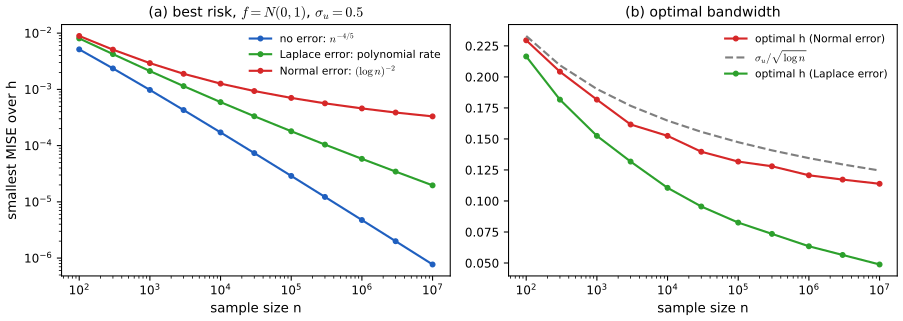
fig_s3. Download: PDF · SVGIf instead \(\sigma_u\to0\) with \(n\), the small-\(\sigma_u\) approach suggests the corrected density estimator \(\hf_n(x)-\frac{\sigma_u^2}{2nh^3}\sum_jK''\big(\frac{\Xb_j-x}{h}\big)\), where \(\hf_n\) is the naive kernel estimate from the \(\Xb_j\) (the book prints \(2nh\) in the denominator; see below).
Filling the gap 10.7: the small-\(\sigma_u\) density correction, and its Fourier meaning p. 233
Derivation
Fix \(X_j\) and expand in \(U_j\): \(h^{-1}K((x-X_j-U_j)/h)=h^{-1}K((x-X_j)/h)-h^{-2}U_jK'(\cdot)+\tfrac12h^{-3}U_j^2K''(\cdot)+\dots\). Taking expectations (the odd terms vanish if \(U\) is symmetric),
\[ \E\hf_n(x)=(K_h*f)(x)+\frac{\sigma_u^2}{2}\,\E\Big[\frac1{h^3}K''\Big(\frac{x-X}h\Big)\Big]+O(\sigma_u^4),\qquad K_h(u)=h^{-1}K(u/h). \]The excess is \(\frac{\sigma_u^2}2\) times the second derivative of the kernel estimate, \(\hf_n''(x)=(nh^3)^{-1}\sum_jK''((x-\Xb_j)/h)\), which is estimated from the data; subtracting it gives
\[ \hf_n(x)-\frac{\sigma_u^2}{2}\hf_n''(x)=\hf_n(x)-\frac{\sigma_u^2}{2nh^3}\sum_{j=1}^nK''\Big(\frac{\Xb_j-x}h\Big), \]with bias \(O(\sigma_u^4)\) beyond the usual kernel bias. (\(K''\) is even, so the sign of its argument is immaterial.) With a Gaussian kernel and \(f=\phi\), \(\sigma_u=0.15\), \(h=0.4\), at \(x=0.3\): the naive estimator's expectation misses the target \(K_h*f\) by \(-3.2\times10^{-3}\), the corrected one by \(-4\times10^{-5}\), and the version printed in the book (\(2nh\), which equals \(h^2\) times the correction) by \(-2.6\times10^{-3}\).
Fourier view. Differentiation twice multiplies the Fourier transform by \(-t^2\), so the corrected estimator is the general formula with multiplier \(m(t)=1+\sigma_u^2t^2/2\): the first two terms of \(1/\psi_U(t)=e^{\sigma_u^2t^2/2}\) for Normal errors. For a Laplace error with variance \(\sigma_u^2\), \(1/\psi_U(t)=1+\sigma_u^2t^2/2\) exactly, so the small-\(\sigma_u\) correction is the deconvolution estimator; in the demo the two curves coincide. For a Cauchy error (no variance) the correction is undefined, but deconvolution still works because \(1/\psi_U(t)=e^{\sigma|t|}\) grows only exponentially in \(|t|\). ∎
See also: kernel density estimation in Chapter 6 of this course and in Probability and Statistical Inference, Section 20.3.
10.2 Inverse Problems
pp. 233–235 In an inverse problem we observe a transformed version of the object of interest, \(Y_i=T_i(r)+\epsilon_i\) (10.24). Following O'Sullivan (1986) take \(T_i(r)=\int K_i(s)r(s)\,\d s\) with a smooth \(K_i\), such as \(K_i(s)=e^{-(s-x_i)^2/2}\):
\[ Y_i=\int K_i(s)r(s)\,\d s+\epsilon_i. \tag{10.25} \]If \(K_i\) is a point mass at \(x_i\) this is ordinary regression. For a linear smoother \(\hr_n(x)=\sum_iY_i\ell_i(x)\) (10.26) the variance is unchanged, \(\sigma^2\sum_i\ell_i(x)^2\), and the mean is \(\int A(x,s)r(s)\,\d s\) with the Backus–Gilbert averaging kernel
\[ A(x,s)=\sum_{i=1}^n\ell_i(x)K_i(s). \tag{10.27} \]Expanding \(r=\sum_{j=1}^k\theta_j\phi_j\) turns (10.25) into a linear model \(Y=Z\theta+\epsilon\) (10.28) with \(Z_{ij}=\int K_i\phi_j\). The least squares estimator usually fails because \(Z^\T Z\) is (nearly) singular: the problem is ill-posed. The regularised estimator \(\hat\theta=LY\), \(L=(Z^\T Z+\lambda I)^{-1}Z^\T\), with \(\lambda\) chosen by cross-validation, is the standard remedy.
Filling the gap 10.8: (10.27), ill-posedness and what cross-validation estimates pp. 234–235
Derivation
(10.27). \(\E\hr_n(x)=\sum_i\ell_i(x)\E Y_i=\sum_i\ell_i(x)\int K_i(s)r(s)\,\d s=\int\big(\sum_i\ell_i(x)K_i(s)\big)r(s)\,\d s\), exchanging a finite sum and an integral. For the basis estimator \(\hr_n(x)=\phi(x)^\T LY\), the weights are \(\ell(x)=L^\T\phi(x)\). The ideal \(A(x,\cdot)\) is a narrow bump at \(x\); how narrow it can be made, at what variance, is the resolution of the experiment.
Ill-posedness. Let \(Z=UDV^\T\) be a singular value decomposition with singular values \(d_1\ge\dots\ge d_k\). Then
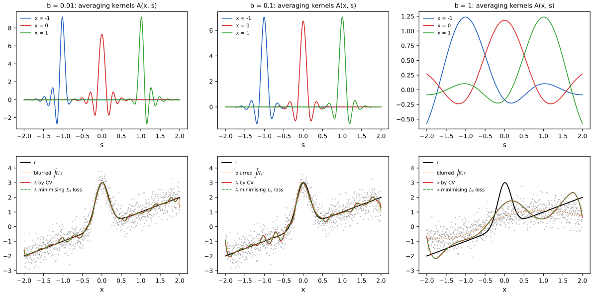
\[ \hat\theta_\lambda=\sum_{m=1}^k\frac{d_m}{d_m^2+\lambda}(u_m^\T Y)\,v_m,\qquad \E\|\hat\theta_0-\theta\|^2=\sigma^2\sum_m d_m^{-2}. \]Smooth kernels \(K_i\) make the \(d_m\) decay quickly (blurring kills high frequencies), so least squares (\(\lambda=0\)) divides noise by tiny numbers. In Exercise 10.6 with \(b=1\), \(Z^\T Z\) has condition number about \(10^{33}\). Ridge replaces \(1/d_m\) by \(d_m/(d_m^2+\lambda)\le1/(2\sqrt\lambda)\): a filter that discards the directions the data cannot see, at the cost of a bias in those directions. This is the same spectral picture as deconvolution, where \(\psi_U\) plays the role of the singular values.
What CV estimates. Leave-one-out cross-validation predicts \(Y_i\) by \(Z_i^\T\hat\theta_{(-i)}\), and for ridge it has the shortcut \(Y_i-Z_i^\T\hat\theta_{(-i)}=(Y_i-\widehat Y_i)/(1-H_{ii})\) with \(H=Z(Z^\T Z+\lambda I)^{-1}Z^\T\) (Sherman–Morrison, as for linear smoothers in Section 5.3; confirmed against brute force). It therefore estimates the prediction error \(n^{-1}\sum_i(\int K_i\hr-\int K_ir)^2\) of the blurred function. The loss we care about, \(\int(\hr-r)^2\), depends on the components of \(r\) in directions with tiny \(d_m\), about which the data carry almost no information; no estimate of it can be reliable without prior assumptions on \(r\). ∎
fig_s4. Download: PDF · SVG10.3 Nonparametric Bayes
p. 235 The book stays frequentist and only points to the literature on Bayesian nonparametrics. The two basic priors are the Gaussian process, for regression functions (covered in the companion course, Bayesian and Probabilistic Machine Learning, Section 6.4), and the Dirichlet process, for distributions. The box below develops the Dirichlet process; Exercise 10.7 studies Gaussian priors in the Normal means model and finds out whether Bayesian credible balls have frequentist coverage.
Filling the gap 10.9: the Dirichlet process p. 235
Definition, posterior and consistency
Definition (Ferguson 1973). Let \(F_0\) be a distribution on \(\R\) and \(\alpha\gt0\). A random distribution \(P\) is a Dirichlet process, \(P\sim\DP(\alpha,F_0)\), if for every finite partition \(A_1,\dots,A_k\) of \(\R\) into measurable sets,
\[ (P(A_1),\dots,P(A_k))\sim\Dir\big(\alpha F_0(A_1),\dots,\alpha F_0(A_k)\big). \]These finite-dimensional laws are consistent (merging cells of a Dirichlet vector adds the parameters, which is the aggregation property of the Dirichlet distribution), so by Kolmogorov's extension theorem such a process exists. Each \(P(A)\) is Beta\((\alpha F_0(A),\alpha(1-F_0(A)))\), so \(\E P(A)=F_0(A)\) and \(\V P(A)=F_0(A)(1-F_0(A))/(\alpha+1)\): \(F_0\) is the prior guess and \(\alpha\) the prior sample size.
Posterior. Let \(X_1,\dots,X_n\given P\) be iid \(P\). Then \(P\given X_{1:n}\sim\DP\big(\alpha+n,\ (\alpha F_0+\sum_i\delta_{X_i})/(\alpha+n)\big)\). Proof for one partition. Given \(P\), the counts \(N_j=\#\{i:X_i\in A_j\}\) are multinomial\((n;P(A_1),\dots,P(A_k))\). The Dirichlet density times the multinomial likelihood is \(\prod_jp_j^{\alpha F_0(A_j)-1}\prod_jp_j^{N_j}\), the kernel of \(\Dir(\alpha F_0(A_j)+N_j)\), which is the claimed finite-dimensional law since \((\alpha F_0+\sum\delta_{X_i})(A_j)=\alpha F_0(A_j)+N_j\). That conditioning on the exact positions \(X_i\) (not just the counts) gives the same answer requires a refinement argument over partitions; see Ferguson (1973) or Ghosh and Ramamoorthi (2003), Chapter 3. ∎
Posterior mean and consistency. With \(A=(-\infty,x]\),
\[ \E(F(x)\given X_{1:n})=\frac{\alpha}{\alpha+n}F_0(x)+\frac{n}{\alpha+n}F_n(x),\qquad \V(F(x)\given X_{1:n})=\frac{\bar F(x)(1-\bar F(x))}{\alpha+n+1}\le\frac1{4(n+1)}, \]where \(\bar F\) is the posterior mean and \(F_n\) the empirical cdf. The posterior mean is a shrinkage of the empirical cdf towards \(F_0\) by a weight \(\alpha/(\alpha+n)\to0\), so by Glivenko–Cantelli (Chapter 2) \(\sup_x|\E(F(x)\given X_{1:n})-F(x)|\to0\) almost surely under any true \(F\), and the posterior variance is \(O(1/n)\): the posterior concentrates at the truth.
Structure. Sethuraman (1994): \(P=\sum_{k\ge1}w_k\delta_{\xi_k}\) with \(\xi_k\) iid \(F_0\), \(w_1=v_1\), \(w_k=v_k\prod_{l\lt k}(1-v_l)\), \(v_k\) iid Beta\((1,\alpha)\) (stick-breaking). So \(P\) is discrete with probability one: a Dirichlet process is a poor prior for a density, and is used instead as the mixing distribution of a mixture, \(f(x)=\int\phi_\sigma(x-\mu)\,\d P(\mu)\), the Dirichlet process mixture. For densities and regression the good behaviour above is not automatic: Diaconis and Freedman (1986) give inconsistent examples, and posterior consistency and rates depend on prior mass near the truth and on the size of the model (Schwartz 1965; Barron, Schervish and Wasserman 1999; Ghosal, Ghosh and van der Vaart 2000).
See also (companion courses): Probability and Statistical Inference, Section 11.2 (the Bayesian method) and 11.9 (strengths and weaknesses); Bayesian and Probabilistic Machine Learning, Section 6.4 (Gaussian processes).
10.4 Semiparametric Inference
pp. 235–236 A semiparametric model has a parametric part of interest and a nonparametric nuisance part, as in the partially linear model
\[ Y=\beta X+r(Z)+\epsilon. \tag{10.29} \]The book suggests regressing \(Y_i-\hr_n(Z_i)\) on \(X_i\), "if \(\hr_n\) is chosen carefully". The care is essential: if \(\hr_n\) is a smooth of \(Y\) on \(Z\), the estimate is inconsistent.
Filling the gap 10.10: the double-residual estimator and its \(\sqrt n\) rate p. 236
Derivation
Assume \(\E(\epsilon\given X,Z)=0\), \(\V(\epsilon\given X,Z)=\sigma^2\), and let \(m_Y(z)=\E(Y\given Z=z)\), \(m_X(z)=\E(X\given Z=z)\), \(V=X-m_X(Z)\) with \(\E V^2\gt0\). Taking conditional expectations of (10.29) given \(Z\): \(m_Y(Z)=\beta m_X(Z)+r(Z)\). Subtracting,
\[ Y-m_Y(Z)=\beta\big(X-m_X(Z)\big)+\epsilon, \]a linear model without intercept in which the nuisance \(r\) has disappeared. Robinson (1988) estimates \(m_Y\) and \(m_X\) by nonparametric smoothers and regresses the residual \(Y-\widehat m_Y(Z)\) on the residual \(X-\widehat m_X(Z)\). With the true \(m\)'s the estimator is \(\beta+\sum V_i\epsilon_i/\sum V_i^2\), so \(\sqrt n(\hb-\beta)\to N(0,\sigma^2/\E V^2)\) by the central limit theorem; the estimation of \(m_Y,m_X\) adds terms such as \(n^{-1/2}\sum(\widehat m_X-m_X)(\widehat m_Y-m_Y)(Z_i)\), which are negligible when both smoothers converge faster than \(n^{-1/4}\) (true for twice-differentiable \(m\)'s in one dimension). The limit variance \(\sigma^2/\E V^2\) is the semiparametric efficiency bound for this model under Normal errors (Bickel et al. 1993; van der Vaart 1998, Chapter 25): \(\beta\) is learned only from the variation of \(X\) not explained by \(Z\).
The naive version. Regressing \(Y-\widehat m_Y(Z)\approx\beta V+\epsilon\) on \(X=m_X(Z)+V\) (with an intercept) gives slope \(\beta\E V^2/\V(X)\), biased towards zero whenever \(X\) depends on \(Z\). Ignoring \(r\) altogether is worse: \(r(Z)\) is an omitted variable correlated with \(X\). In Figure 10.S5, \(\E V^2/\V X=1/3\), the naive estimates average 0.45 (1/3 plus a contribution from the smoothing bias of \(\widehat m_Y\)), and the double-residual estimates average 1.02 with standard deviation 0.068, against the efficient \(\sigma/\sqrt{n\E V^2}=0.071\). An equivalent form of the "careful" \(\hr_n\) is \(\widehat m_Y-\hb\,\widehat m_X\). ∎
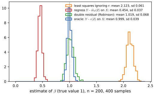
fig_s5. Download: PDF · SVGSee also (companion course): Statistical Learning, Section 9.1 (additive models and backfitting); backfitting a partially linear model converges to the same estimator (Speckman 1988).
10.5 Correlated Errors
p. 236 With positively correlated errors, cross-validation tends to choose bandwidths that are far too small. Modified cross-validation leaves out a block of neighbouring observations; partitioned cross-validation splits the data into interleaved subsamples, cross-validates within each, and averages (Chu and Marron 1991; Opsomer, Wang and Yang 2001).
Filling the gap 10.11: the bias of cross-validation under correlation p. 236
Derivation
Let \(Y=r+\epsilon\) with \(\cov(\epsilon)=\Gamma\), \(\Gamma_{ij}=\gamma(i-j)\) (fixed design \(x_1\lt\dots\lt x_n\)). Let \(L\) be the leave-one-out smoother matrix: row \(i\) gives \(\hr_{(-i)}(x_i)=\sum_jL_{ij}Y_j\), with \(L_{ii}=0\). Then \(Y-LY=(I-L)r+(I-L)\epsilon\) and
\[ \E\,\mathrm{CV}=\frac1n\|(I-L)r\|^2+\frac1n\Tr\big((I-L)\Gamma(I-L)^\T\big)=\underbrace{\frac1n\|(I-L)r\|^2+\frac1n\Tr(L\Gamma L^\T)}_{\text{risk of }\hr_{(-i)}}+\gamma(0)-\frac2n\sum_i\sum_{j\ne i}L_{ij}\gamma(i-j). \]With independent errors the last term is zero and CV estimates the risk plus \(\sigma^2\) (Section 5.3). With \(\gamma(k)\gt0\) for small \(|k|\), the last term is negative, and it grows in size as \(h\) shrinks, because a small bandwidth puts the weights \(L_{ij}\) on the nearest neighbours, whose errors are most correlated with \(\epsilon_i\). The smoother "predicts" \(\epsilon_i\) from its correlated neighbours, CV rewards it, and the minimiser drifts to tiny \(h\). For AR(1) errors with \(\phi=0.6\), \(n=100\) and \(h=0.02\) the term equals \(-0.21\) against \(\gamma(0)=0.25\) (the closed form agreed with a simulation of \(\E\,\mathrm{CV}\) to 0.6%). Leaving out \(|i-j|\le l\) sets those \(L_{ij}\) to zero, so the term becomes \(-\frac2n\sum_{|i-j|\gt l}L_{ij}\gamma(i-j)\), negligible once \(\gamma(k)\) is small for \(|k|\gt l\). ∎
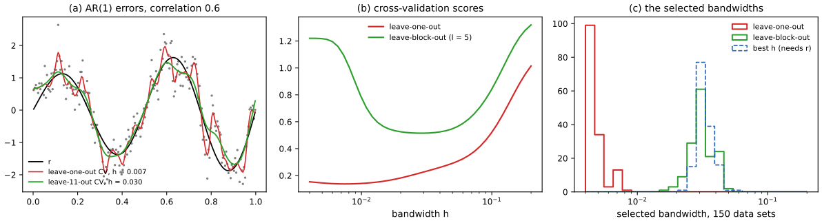
fig_s6. Download: PDF · SVGSee also (companion course): Statistical Learning, Section 7.10 (cross-validation).
10.6 Classification
pp. 236–237 With \(Y\in\{0,1\}\), a classifier \(h\) has risk \(L(h)=\P(Y\ne h(X))\). The optimal rule, the Bayes rule, is \(h^*(x)=\I(r(x)\ge1/2)\) with \(r(x)=\E(Y\given X=x)\), and the plug-in rule is \(\hat h(x)=\I(\hr_n(x)\ge1/2)\). A poor \(\hr_n\) can still classify well: if \(r(x)=0.6\) and \(\hr_n(x)=0.9\), both rules say 1.
Filling the gap 10.12: the Bayes rule is optimal, and the plug-in bound p. 237
Proof
For any \(h\), conditioning on \(X\): \(\P(Y\ne h(X)\given X=x)=r(x)\I(h(x)=0)+(1-r(x))\I(h(x)=1)\), which is minimised pointwise by choosing 1 when \(r(x)\ge1-r(x)\), i.e. \(h^*\). Moreover
\[ L(h)-L(h^*)=\E\big[\,|2r(X)-1|\,\I(h(X)\ne h^*(X))\big]. \]If \(\hat h(x)\ne h^*(x)\), then \(r(x)\) and \(\hr_n(x)\) lie on opposite sides of \(1/2\) (or one equals it), so \(|2r(x)-1|=2|r(x)-\tfrac12|\le2|r(x)-\hr_n(x)|\). Hence
\[ L(\hat h)-L(h^*)\le2\,\E\big|\hr_n(X)-r(X)\big|\le2\big(\E(\hr_n(X)-r(X))^2\big)^{1/2}. \]The bound is crude: errors far from the boundary \(\{r=1/2\}\) cost nothing, and errors near it cost little because \(|2r-1|\) is small there. Classification is "easier" than regression in this sense. In Figure 10.S7 the excess risk is minimised at \(h=0.076\), the integrated squared error of \(\hr_n\) at \(h=0.047\): the classifier tolerates oversmoothing, because only the location of the crossings of 1/2 matters. ∎
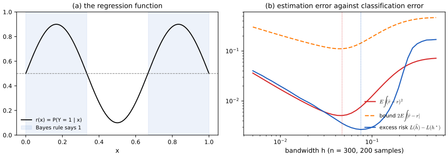
fig_s7. Download: PDF · SVGSee also (companion courses): Probability and Statistical Inference, Section 22.2 (error rates and the Bayes classifier); Statistical Learning, Section 2.4 and 4.4 (logistic regression).
10.7 Sieves
p. 237 A sieve is a sequence of models of growing complexity indexed by \(n\), for instance polynomials of degree \(p(n)\) (Grenander 1981; Geman and Hwang 1982). Choosing the complexity is a bias–variance trade-off, like choosing a bandwidth.
Filling the gap 10.13: the risk of a linear sieve and the best dimension p. 237
Derivation
Take a fixed design and \(k\) basis vectors orthonormal on it (for the design \(x_i=(i-\tfrac12)/n\), the discrete cosine basis \(\sqrt{2/n}\cos(\pi j x_i)\), \(j\ge1\), plus the constant, is exactly orthonormal). Write \(r(x_i)=\sqrt n\sum_j\theta_j\varphi_j(x_i)\) in this basis. Least squares on the first \(k\) vectors keeps the first \(k\) empirical coefficients, each the true one plus independent \(N(0,\sigma^2/n)\) noise, so
\[ \frac1n\sum_i\E(\hr_n(x_i)-r(x_i))^2=\frac{\sigma^2k}{n}+\sum_{j\gt k}\theta_j^2. \]If \(\sum_jj^{2s}\theta_j^2\le c^2\) (a Sobolev ellipsoid, Chapter 7), the tail is at most \(c^2k^{-2s}\), and minimising \(\sigma^2k/n+c^2k^{-2s}\) gives \(k\asymp n^{1/(2s+1)}\) and risk \(\asymp n^{-2s/(2s+1)}\), the minimax rate over the ellipsoid. The function of Figure 10.S8 has a kink, so \(|\theta_j|\asymp j^{-2}\), the tail is \(\asymp k^{-3}\), and the best \(k\) grows like \(n^{1/4}\) with risk \(n^{-3/4}\). The formula above was confirmed by simulation. Choosing \(k\) from the data (by \(C_p\), cross-validation or penalised likelihood) is the subject of Chapter 8; the general theory of sieve and penalised estimators uses entropy bounds (Shen and Wong 1994; van de Geer 2000). ∎
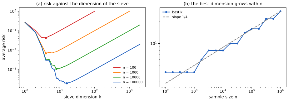
fig_s8. Download: PDF · SVG10.8 Shape-Restricted Inference
pp. 237–238 Shape restrictions can replace smoothness. Let \(Y_i=r(x_i)+\epsilon_i\), \(x_1\lt\dots\lt x_n\), with \(r\) nondecreasing. The isotonic regression estimator minimises \(\sum_i(Y_i-r(x_i))^2\) over nondecreasing \(r\). With \(P_0=(0,0)\), \(P_j=(j,\sum_{i\le j}Y_i)\) and \(G\) the greatest convex minorant of \(P_0,\dots,P_n\), the solution is \(\hr_n(x_j)=G(j)-G(j-1)\), the left derivative of \(G\) at \(j\); the pool-adjacent-violators (PAV) algorithm computes it in \(O(n)\) operations. Zhang (2002): with \(R_{n,p}(r)=(n^{-1}\sum_i\E|\hr_n(x_i)-r(x_i)|^p)^{1/p}\), \(1\le p\le3\), and \(V(r)\) the total variation,
\[ 0.64+o(1)\le\frac{n^{1/3}}{\sigma^{2/3}V^{1/3}}\sup_{V(r)\le V}R_{n,p}(r)\le M_p+o(1). \tag{10.30} \]Filling the gap 10.14: the convex minorant solves the problem, and PAV computes it p. 238
Proof
Write \(\theta_i=r(x_i)\); the problem is the projection of \(Y\) onto the closed convex cone \(\mathcal C=\{\theta:\theta_1\le\dots\le\theta_n\}\). Projection onto a cone. \(\hat\theta=\Pi_{\mathcal C}Y\) if and only if \(\hat\theta\in\mathcal C\), \(\langle Y-\hat\theta,\hat\theta\rangle=0\) and \(\langle Y-\hat\theta,\theta\rangle\le0\) for all \(\theta\in\mathcal C\) (the variational inequality \(\langle Y-\hat\theta,\theta-\hat\theta\rangle\le0\), applied with \(\theta=2\hat\theta\) and \(\theta=0\), gives the equality; the rest follows). The cone is generated by \(\pm\mathbf1\) and the step vectors \(e^{(j)}=(0,\dots,0,1,\dots,1)\) (ones from position \(j\), \(j=2,\dots,n\)), so the last condition reads: \(\sum_{i}(Y_i-\hat\theta_i)=0\) and \(\sum_{i\ge j}(Y_i-\hat\theta_i)\le0\) for all \(j\).
The minorant satisfies them. Let \(S_j=\sum_{i\le j}Y_i\) and \(\hat\theta_j=G(j)-G(j-1)\), so \(G(j)=\sum_{i\le j}\hat\theta_i\). (a) \(G\) is convex and piecewise linear, so its slopes increase: \(\hat\theta\in\mathcal C\). (b) \(P_0\) and \(P_n\) are vertices of the minorant, so \(G(0)=0\), \(G(n)=S_n\), and \(G(j)\le S_j\) for all \(j\). Then \(\sum_{i\ge j}(Y_i-\hat\theta_i)=(S_n-S_{j-1})-(G(n)-G(j-1))=G(j-1)-S_{j-1}\le0\), with equality for \(j=1\). (c) By summation by parts, with \(D_j=S_j-G(j)\ge0\) and \(D_0=D_n=0\),
\[ \langle Y-\hat\theta,\hat\theta\rangle=\sum_{j=1}^{n}(D_j-D_{j-1})\hat\theta_j=\sum_{j=1}^{n-1}D_j(\hat\theta_j-\hat\theta_{j+1}). \]\(\hat\theta_j\ne\hat\theta_{j+1}\) only where \(G\) has a vertex at \(j\), and there \(D_j=0\); so every term vanishes. Hence \(\hat\theta=\Pi_{\mathcal C}Y\), unique because the projection onto a closed convex set is unique. ∎
Min-max formula. Equivalently \(\hat\theta_i=\max_{s\le i}\min_{t\ge i}\bar Y_{s:t}\), the average of \(Y_s,\dots,Y_t\) (Robertson, Wright and Dykstra 1988, Theorem 1.4.4): slopes of the lower convex hull are max-min of chord slopes.
PAV. Process the points from left to right, keeping a stack of blocks with increasing means; push each new point as a block, and while the last block's mean is below the previous block's mean, merge them (the merged mean is the weighted average). The key fact is that if two adjacent blocks, each known to be constant in the solution, have decreasing means, the solution is constant on their union: otherwise moving the two levels towards each other lowers the sum of squares without breaking monotonicity. Each merge reduces the number of blocks, so the total work is \(O(n)\). The book's description joins segments only from \(P_0\) onward and omits the backward merging (see the notes on the book). The code and the demo implement the stack version; it agrees with the min-max formula, with the slopes of the convex minorant and with scikit-learn's implementation.
Filling the gap 10.15: why the rate is \(n^{-1/3}\), and the form of (10.30) p. 238
Heuristic and the exact limit
Near a point \(x\) where \(r'(x)\gt0\), the fit is an average over a block of about \(m\) neighbouring points. Its noise is \(\sigma/\sqrt m\); its bias is the variation of \(r\) across the block, about \(r'(x)m/n\). The algorithm pools until the noise no longer dominates the trend, so \(\sigma/\sqrt m\asymp r'(x)m/n\), i.e. \(m\asymp(\sigma n/r'(x))^{2/3}\) and the error is \(\asymp(\sigma^2r'(x)/n)^{1/3}\). Averaging over \(x\in[0,1]\) and using Jensen's inequality for the concave map \(u\mapsto u^{1/3}\),
\[ \int_0^1\big(\sigma^2r'(x)/n\big)^{1/3}\d x\le\sigma^{2/3}n^{-1/3}\Big(\int_0^1r'(x)\,\d x\Big)^{1/3}=\sigma^{2/3}V^{1/3}n^{-1/3}, \]exactly the normalisation of (10.30). Rigorously, Brunk (1970) showed \(n^{1/3}(\hr_n(x)-r(x))\to(4\sigma^2r'(x))^{1/3}\,\mathbb Z\) in distribution (for a uniform design on \([0,1]\)), where \(\mathbb Z\) is the location of the minimum of two-sided Brownian motion plus \(t^2\) (Chernoff's distribution). The constants in (10.30) are Zhang's (2002) and are quoted, not proved, here. In Figure 10.S9 the root mean squared error falls with slope \(-0.35\) on the log–log scale, and \(n^{1/3}R_{n,2}/(\sigma^2V)^{1/3}\) stays between 0.85 and 0.95 from \(n=50\) to 10000. If \(r\) is constant, \(V=0\) and the risk is much smaller, of order \(\sigma\sqrt{\log n/n}\).
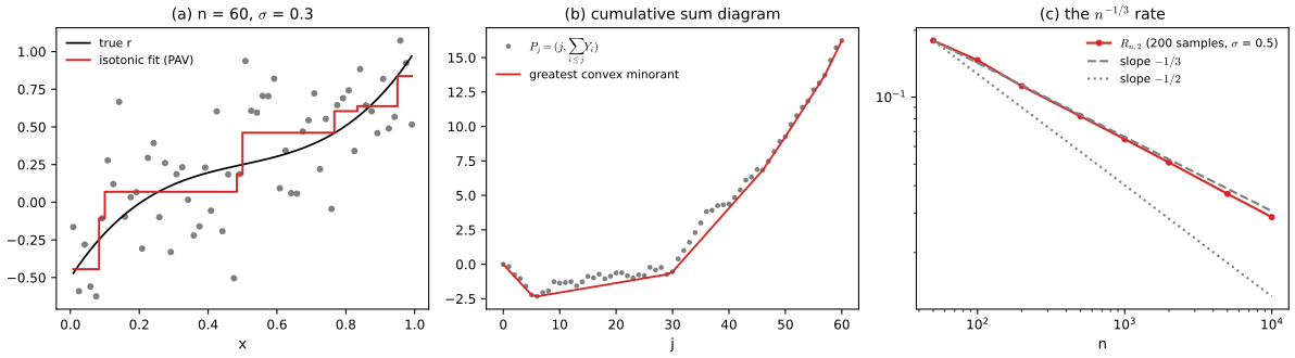
fig_s9. Download: PDF · SVGOptimal confidence bands for monotone functions are in Dümbgen (2003) and Dümbgen and Johns (2004), and for monotone densities in Hengartner and Stark (1995).
10.9 Testing
pp. 238–239 In the Normal means model \(Y_i=\theta_i+\epsilon_i\), \(\epsilon_i\sim N(0,1)\), \(i=1,\dots,n\), test \(H_0:\theta=0\) against \(H_1:\theta\in V_n=\{\theta:\|\theta\|_p\ge R_n\}\). For a test \(\psi\) let \(\alpha_n(\psi)=\E_0\psi\), \(\beta_n(\psi,\theta)=\E_\theta(1-\psi)\) and \(\gamma_n=\inf_\psi(\alpha_n(\psi)+\sup_{\theta\in V_n}\beta_n(\psi,\theta))\). Ingster showed \(\gamma_n\to0\) iff \(R_n/R_n^*\to\infty\) and \(\gamma_n\to1\) iff \(R_n/R_n^*\to0\), with
\[ R_n^*=\begin{cases}n^{1/p-1/4}&p\le2,\\ n^{1/(2p)}&p\gt2.\end{cases} \]Filling the gap 10.16: Ingster's boundary for \(p=2\), both directions p. 239
Proof
Upper bound: the \(\chi^2\) test. Let \(T=\sum_iY_i^2\). Under \(\theta\), \(T\) is noncentral \(\chi^2_n(\|\theta\|^2)\) with mean \(n+\|\theta\|^2\) and variance \(2n+4\|\theta\|^2\). Reject when \(T\gt n+z\sqrt{2n}\); then \(\alpha_n\to1-\Phi(z)\) by the central limit theorem. For \(\|\theta\|\ge R_n\) with \(R_n^2/\sqrt n\to\infty\), Chebyshev gives
\[ \beta_n(\theta)=\P_\theta(T\le n+z\sqrt{2n})\le\frac{2n+4\|\theta\|^2}{(\|\theta\|^2-z\sqrt{2n})^2}\to0 \]uniformly over \(V_n\) (the bound decreases in \(\|\theta\|\) once \(\|\theta\|^2\gt z\sqrt{2n}\)). Letting \(z\to\infty\) slowly, \(\gamma_n\to0\) whenever \(R_n/n^{1/4}\to\infty\).
Lower bound: a random alternative. Put a prior \(\pi\) on \(V_n\): \(\theta=a\varepsilon\), \(a=R_n/\sqrt n\), \(\varepsilon\) uniform on \(\{-1,1\}^n\), so \(\|\theta\|_2=R_n\) exactly. For any test, \(\alpha_n+\sup_{V_n}\beta_n\ge\alpha_n+\int\beta_n\,\d\pi\ge1-\TV(P_0,P_\pi)\), where \(P_\pi\) is the mixture. With likelihood ratio \(L=\d P_\pi/\d P_0=\prod_i\cosh(aY_i)e^{-a^2/2}\), the Cauchy–Schwarz inequality gives \(\TV\le\tfrac12(\E_0L^2-1)^{1/2}\), and taking the expectation over two independent copies \(\varepsilon,\varepsilon'\),
\[ \E_0L^2=\E_{\varepsilon,\varepsilon'}\prod_i\E_0\,e^{a(\varepsilon_i+\varepsilon_i')Y_i-a^2}=\E\prod_ie^{a^2\varepsilon_i\varepsilon_i'}=\cosh(a^2)^n\le e^{na^4/2}=e^{R_n^4/(2n)}, \]using \(\E_0e^{cY}=e^{c^2/2}\) and \(\cosh u\le e^{u^2/2}\). If \(R_n/n^{1/4}\to0\), then \(\E_0L^2\to1\), \(\TV\to0\) and \(\gamma_n\to1\). ∎
Both bounds are exact functions of \(R_n/n^{1/4}\) in the limit (Figure 10.S10): the \(\chi^2\) test has power \(1-\Phi(z_\alpha-c^2/\sqrt2)\) at \(\|\theta\|=cn^{1/4}\). Other \(p\). For \(p\lt2\) the hardest alternatives are spread out: \(\theta_i=R_nn^{-1/p}\) has \(\|\theta\|_2=R_nn^{1/2-1/p}\), which is at the \(\ell_2\) boundary \(n^{1/4}\) when \(R_n=n^{1/p-1/4}\). For \(p\gt2\) they are sparse: about \(\sqrt n\) coordinates of size of order one are invisible to the \(\chi^2\) test (sum of squares \(\sqrt n\)) and too small for a max test, and have \(\ell_p\) norm \(n^{1/(2p)}\). Proofs are in Ingster and Suslina (2003). This critical radius is also what limits the radius of adaptive confidence balls in Chapter 7.
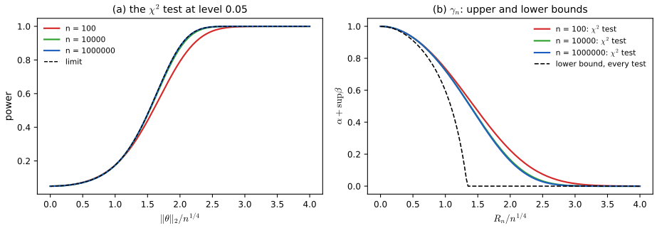
fig_s10. Download: PDF · SVGQualitative hypotheses (\(f\) monotone, positive, convex) are convex cones: closed under addition and under multiplication by nonnegative scalars. For testing that \(r\) is nonincreasing when \(r\) belongs to the Hölder class \(\{|r(x)-r(y)|\le L|x-y|^s\}\), \(0\lt s\le1\), there are tests with uniformly large power against every \(r\) at distance at least of order \(L^{1/(1+2s)}n^{-s/(1+2s)}\) from the null (Dümbgen and Spokoiny 2001, where the distance is in sup norm and a \(\log n\) factor appears; Baraud, Huet and Laurent 2003; Juditsky and Nemirovski 2002).
Filling the gap 10.17: what "cone" buys p. 239
Remark
For a convex cone \(\mathcal C\), the least squares fit under the null is the projection \(\Pi_{\mathcal C}Y\), and the likelihood ratio statistic in the Normal model is \(\|Y\|^2-\|Y-\Pi_{\mathcal C}Y\|^2=\|\Pi_{\mathcal C}Y\|^2\) when the null is \(\theta=0\), or the distance \(\|Y-\Pi_{\mathcal C}Y\|^2\) when the null is \(\theta\in\mathcal C\). The identity \(\langle Y-\Pi Y,\Pi Y\rangle=0\) used in Filling the gap 10.14 holds for every closed convex cone, and the null distribution of \(\|Y-\Pi_{\mathcal C}Y\|^2\) at \(\theta=0\) is a mixture of \(\chi^2\) distributions (the "chi-bar-squared" distribution; Robertson, Wright and Dykstra 1988). The least favourable point of the null is the apex \(\theta=0\), because \(\|Y-\Pi_{\mathcal C}Y\|\) is stochastically largest there; this is what makes cone hypotheses tractable. Closure under addition alone, as the book says, does not make a set a cone (the set of nonnegative integers is closed under addition).
10.10 Computational Issues
p. 240 Nonparametric methods shine on large data sets, and that is exactly where naive implementations (\(n\) kernel evaluations at each of \(m\) points) become slow. Binning (Fan and Marron 1994; Hall and Wand 1996) replaces the data by counts on a grid; k-d trees (Loader 1999, Chapter 12) partition the data so that distant points are summarised in bulk.
Filling the gap 10.18: why binning is accurate and fast p. 240
Derivation
Round each \(X_i\) to the nearest point \(g_i\) of a grid of spacing \(\delta\), so \(|X_i-g_i|\le\delta/2\). For a kernel estimate with differentiable \(K\), by the mean value theorem
\[ \Big|\frac1{nh}\sum_iK\Big(\frac{x-g_i}h\Big)-\frac1{nh}\sum_iK\Big(\frac{x-X_i}h\Big)\Big|\le\frac{\delta\,\sup|K'|}{2h^2}, \]uniformly in \(x\); with \(\delta\) a small fraction of \(h^2\) the error is negligible next to the statistical error. (Linear binning, which splits each point between its two neighbours, makes the first-order error cancel and achieves \(O(\delta^2/h^3)\).) On the grid the estimate is a discrete convolution of the \(M\) bin counts with the kernel weights \(K(k\delta/h)\), \(|k|\le c h/\delta\): \(O(M\,h/\delta)\) operations directly or \(O(M\log M)\) with the fast Fourier transform, after an \(O(n)\) binning pass, instead of \(O(nm)\). Local polynomial fits only need the binned moments \(\sum_iK(\cdot)(g_i-x)^l\) and \(\sum_iK(\cdot)(g_i-x)^lY_i\), so the same trick applies to regression and to all bandwidths at once.
10.11 Exercises
Exercise 10.1. In the "errors in \(Y\)" model \(Y_i=r(X_i)+\epsilon_i\), \(Y^\bullet_i=Y_i+U_i\) with \(\E(U_i)=0\), we observe \((X_i,Y_i^\bullet)\). How does this affect the estimation of \(r\)?
Solution
If \(\E(U\given X)=0\) (for instance \(U\) independent of \(X\)), then \(\E(Y^\bullet\given X=x)=r(x)+\E(\epsilon\given X=x)+\E(U\given X=x)=r(x)\): the regression function is unchanged, and \(Y^\bullet=r(X)+\epsilon'\) with \(\epsilon'=\epsilon+U\) is an ordinary regression model with noise variance \(\sigma^2+\sigma_u^2\) (if \(U\) and \(\epsilon\) are uncorrelated). So every estimator of Chapter 5 remains consistent with the same bias; only the variance increases, by the factor \((\sigma^2+\sigma_u^2)/\sigma^2\). The optimal bandwidth grows accordingly (for a local linear smoother, \(h_*\propto(\sigma^2+\sigma_u^2)^{1/5}n^{-1/5}\)), cross-validation and variance estimation work unchanged (they estimate the total noise variance), and confidence bands widen. Error in the response is a variance problem; error in the covariate (Section 10.1) is a bias problem. The exception is error correlated with \(X\) (\(\E(U\given X)\ne0\), e.g. a miscalibrated instrument), which shifts the regression function and cannot be detected from the data.
Exercise 10.2. Prove (10.1).
Solution
See Filling the gap 10.1: the slope is the ratio of the sample covariance of \((\Xb,Y)\) and the sample variance of \(\Xb\); by the strong law these converge to \(\beta_1\sigma_x^2\) and \(\sigma_x^2+\sigma_u^2\), and the ratio converges by continuity. A simulation with \(n=200{,}000\), \(\beta_1=1.5\), \(\sigma_u=0.7\) gives 1.0056 against \(\lambda\beta_1=1.0067\).
Exercise 10.3. Prove (10.20).
Solution
See Filling the gap 10.5: the Fourier transform of the kernel estimate is \(\psi_K(th)\) times the empirical characteristic function; substituting it in (10.19), exchanging sum and integral and changing variables \(u=th\) gives (10.20) with the kernel (10.21).
Exercise 10.4. Draw \(X_1,\dots,X_{100}\sim N(0,1)\). (a) Estimate the density with a kernel estimator. (b) Let \(W_i=X_i+\sigma_uU_i\), \(U_i\sim N(0,1)\); compute the uncorrected and corrected density estimators from the \(W_i\) and compare them, for several \(\sigma_u\). (c) Repeat (b) with Cauchy \(U_i\).
Solution
Method. All estimators are computed by Fourier inversion with \(\psi_K(s)=(1-s^2)^3\) (Filling the gap 10.6): naive (\(m=1\)), deconvolution (\(m=1/\psi_U\), equation (10.20)) and small-\(\sigma_u\) corrected (\(m=1+\sigma_u^2t^2/2\)). Since \(f\) is known here, each bandwidth is the minimiser of the exact MISE for that estimator (an oracle choice; in practice one would use a plug-in rule or the deconvolution cross-validation of Stefanski and Carroll 1990). One sample, the same \(X_i\) throughout.
case estimator \(h\) exact MISE ISE (this sample) (a) \(X\) observed kernel 0.17 0.0052 0.0026 (b) Normal, \(\sigma_u=0.25\) naive 0.17 0.0062 0.0029 deconvolution 0.19 0.0060 0.0028 small \(\sigma_u\) 0.19 0.0060 0.0027 (b) Normal, \(\sigma_u=0.5\) naive 0.15 0.0100 0.0050 deconvolution 0.23 0.0089 0.0038 small \(\sigma_u\) 0.22 0.0086 0.0037 (c) Cauchy, scale 0.25 naive 0.14 0.0155 0.0111 deconvolution 0.22 0.0095 0.0063 Findings (Figure 10.S2). With \(n=100\) the error variance \(\sigma_u^2=0.06\) is too small to matter: all estimates are within sampling noise of each other. At \(\sigma_u=0.5\) the naive estimate is visibly too flat (it estimates \(N(0,1.25)\)), and both corrections help, the small-\(\sigma_u\) one slightly more at this sample size because its multiplier grows only quadratically. The corrected estimators need a larger bandwidth, as the theory predicts. With Cauchy errors the naive estimate has heavy tails and the worst risk; the small-\(\sigma_u\) correction does not exist (no variance) but deconvolution works and cuts the MISE by 40%. With Normal errors, increasing \(n\) helps deconvolution only slowly (Figure 10.S3).
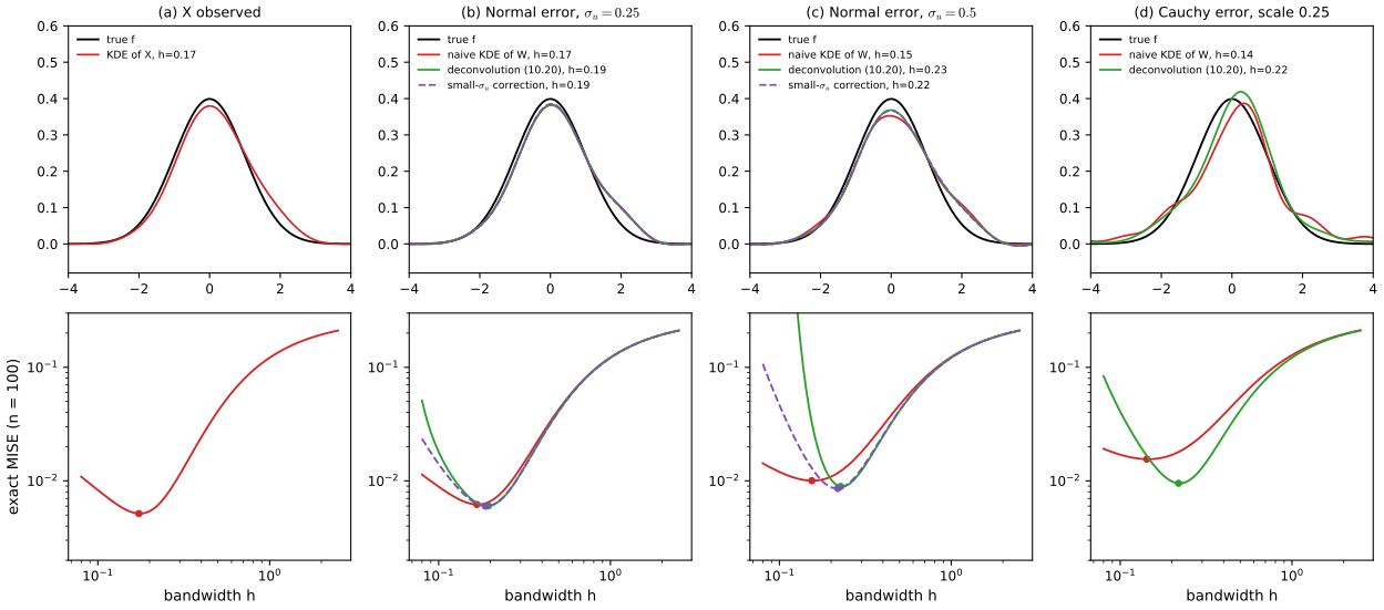
Figure 10.S2 (supplementary). Exercise 10.4: estimates from one sample of 100 (top) and exact MISE curves (bottom), with each bandwidth at the minimum of its curve. Code: fig_s2. Download: PDF · SVG▶ DemoExercise 4(b)The same set-up, with other samples, errors and bandwidths; preset 4 is part (c).Exercise 10.5. Generate 1000 observations from \(Y_i=r(X_i)+\sigma_\epsilon\epsilon_i\), \(W_i=X_i+\sigma_uU_i\), with \(r(x)=x+3e^{-16x^2}\), \(X_i\sim\mathrm{Unif}(-2,2)\), \(\sigma_\epsilon=0.5\), \(\sigma_u=0.1\). (a) Kernel regression of \(Y\) on \(X\) with \(h\) by cross-validation: \(r_n^*\). (b) Kernel regression of \(Y\) on \(W\) with the same \(h\): \(\hr_n\). (c) The corrected estimator (10.14). (d) Compare. (e) Find a good bandwidth from \((W,Y)\) only and compare.
Solution
Method. Nadaraya–Watson with a Gaussian kernel. (a) Leave-one-out CV on \((X,Y)\) over 40 bandwidths gives \(h=0.059\). (c) The correction of Filling the gap 10.4, with \(r(W_i)\) replaced by the pilot \(\hr_n(W_i)\). I also computed SIMEX (\(\rho=0,0.5,\dots,2\), \(B=20\), quadratic extrapolation pointwise). (e) SIMEX cross-validation: compute the CV score of \((W+\sqrt\rho\,\sigma_uZ,Y)\) for \(\rho=0,0.5,\dots,2\) (8 pseudo-samples each), extrapolate the score curve quadratically to \(\rho=-1\) at each \(h\), and minimise; this mimics the CV score we would get from the true \(X\).
Results (integrated squared error over \([-1.9,1.9]\)): \(r_n^*\) 0.027; naive \(\hr_n\) 0.107; corrected (10.14) 0.062; SIMEX 0.059; (e) \(h=0.086\) and, with the correction, 0.078. (d) The naive fit flattens the peak at 0 from 3 to about 2.5 and fills the dips beside it, exactly the \(\sigma_u^2r''/2\) pattern of (10.3) (panel (c) of Figure 10.S1); both corrections restore most of the peak, at the price of more wiggle elsewhere (they add variance). (e) The extrapolated CV curve has the shape of the true one but its minimum is at the same place as plain CV on \((W,Y)\), larger than the oracle 0.059: choosing \(h\) under measurement error is hard, as the book says, and an active research topic (Delaigle and Hall 2008 propose a SIMEX approach of this kind).
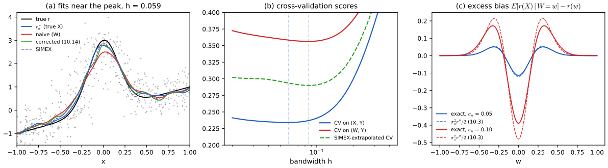
Figure 10.S1 (supplementary). Exercise 10.5: (a) fits near the peak; (b) cross-validation scores; (c) the exact excess bias \(\E(r(X)\given W=w)-r(w)\) and its approximation (10.3). Code: fig_s1,ex5_fit. Download: PDF · SVGExercise 10.6. Generate 1000 observations from \(Y_i=\int K_i(s)r(s)\,\d s+\sigma\epsilon_i\) with \(r(x)=x+3e^{-16x^2}\), \(\sigma=0.5\), \(K_i(s)=e^{-(s-x_i)^2/b^2}\), \(x_i=4(i/n)-2\), for \(b=0.01,0.1,1\). (a) Plot the Backus–Gilbert averaging kernel for several \(x\) and interpret. (b) Estimate \(r\) by the method of this section.
Solution
Set-up. The book writes \(\int K_i(s)\,\d s\); the integrand must contain \(r(s)\), as in (10.25). Taken literally, \(K_i\) has mass \(b\sqrt\pi\), so for \(b=0.01\) the signal is \(0.018\,r\) buried in noise of sd 0.5. I normalise \(K_i\) to integrate to one, so the three cases differ only in the amount of blur; \(s\) ranges over \([-2,2]\). Basis: 40 cubic B-splines on \([-2,2]\); \(Z_{ij}=\int K_i\phi_j\) by the trapezoid rule on 8001 points; ridge estimator with \(\lambda\) by leave-one-out CV (shortcut of Filling the gap 10.8).
(a) (Figure 10.S4, top.) For \(b=0.01\) and \(0.1\), \(A(x,\cdot)\) is a sharp peak at \(x\) of width about 0.1 with small oscillating side lobes: the estimate at \(x\) averages \(r\) over a small window, like an ordinary smoother. For \(b=1\), \(A(x,\cdot)\) is a broad bump of width about 1 with negative lobes: \(\hr(x)\) is a heavily blurred average of \(r\), and no choice of \(\lambda\) can make it narrow without exploding variance. (b) CV chooses \(\lambda=0.25\), \(0.25\) and \(0.025\). The \(L_2\) losses \(\int(\hr-r)^2\) are 0.038, 0.120 and 0.996; for \(b=0.1\) the \(\lambda\) minimising the \(L_2\) loss is 0.40 (loss 0.113), so CV is close to optimal there; for \(b=0.01\) and \(1\) the two choices coincide. With \(b=1\) the peak of \(r\) is gone: the blurred signal \(\int K_ir\) shows only a gentle rise (orange in the figure), the singular values of \(Z\) span 33 orders of magnitude, and the estimate is a smooth curve with spurious wiggles that misses the peak entirely. Information destroyed by blurring is not recovered by any amount of regularisation.
Exercise 10.7. In the infinite Normal means model \(Y_i=\theta_i+n^{-1/2}\epsilon_i\), \(i=1,2,\dots\), with \(\theta\) in the Sobolev ellipsoid \(\{\sum\theta_j^2j^2\le c^2\}\), put independent priors \(\theta_i\sim N(0,\tau_i^2)\). (a) Find the posterior and the posterior mean \(\hat\theta\). (b) Find conditions on \(\tau_i^2\) for consistency, \(\P_\theta(\|\hat\theta-\theta\|\gt\epsilon)\to0\). (c) With \(\theta_j=j^{-4}\) and \(n=100\), find \(b_n\) with \(\P(\|\theta-\hat\theta\|\le b_n\given\text{data})=0.95\), and estimate the frequentist coverage of \(B_n=\{\theta:\|\theta-\hat\theta\|\le b_n\}\) by simulation. (d) Repeat for \(\theta=0\).
Solution
(a) Coordinates are independent a posteriori, and each is a Normal–Normal update with prior precision \(\tau_i^{-2}\) and data precision \(n\):
\[ \theta_i\given Y\sim N\big(s_iY_i,\ v_i\big),\qquad s_i=\frac{\tau_i^2}{\tau_i^2+1/n},\qquad v_i=\frac{\tau_i^2/n}{\tau_i^2+1/n}=\frac{s_i}{n}, \]so \(\hat\theta_i=s_iY_i\), a linear shrinkage estimator (Chapter 7).
(b) \(\hat\theta_i-\theta_i=-(1-s_i)\theta_i+s_i\epsilon_i/\sqrt n\), so
\[ \E_\theta\|\hat\theta-\theta\|^2=\sum_i(1-s_i)^2\theta_i^2+\sum_i\frac{s_i^2}{n}. \]The first sum tends to 0 for every \(\theta\in\ell_2\) and every choice of \(\tau_i\gt0\), by dominated convergence (\((1-s_i)^2\theta_i^2\le\theta_i^2\) and \(1-s_i\to0\) for each \(i\) as \(n\to\infty\)). With \(u_i=n\tau_i^2\), the second sum is \(n^{-1}\sum_iu_i^2/(1+u_i)^2\), which lies between \(\frac14\sum_i\min(1/n,n\tau_i^4)\) and \(\sum_i\min(1/n,n\tau_i^4)\). So the posterior mean is consistent (in mean square, hence in probability by Markov's inequality) if and only if \(\sum_i\min(1/n,n\tau_i^4)\to0\). A simple sufficient condition is \(\sum_i\tau_i^2\lt\infty\) (since \(\min(1/n,n\tau^4)\le\tau^2\cdot\min(1/(n\tau^2),n\tau^2)\le\tau^2\), and each term tends to 0, dominated convergence applies); for \(\tau_i^2=i^{-2a}\) the condition is equivalent to \(a\gt1/2\). The posterior itself contracts (posterior spread \(\sum_iv_i\to0\)) if and only if \(\sum_i\tau_i^2\lt\infty\), because \(v_i\asymp\min(\tau_i^2,1/n)\).
(c), (d) \(b_n\) does not depend on the data: \(\|\theta-\hat\theta\|^2\given Y\sim\sum_iv_iZ_i^2\). I used \(\tau_j^2=j^{-2a}\) for \(a=1,1.5,2,3,5\), the first 2000 coordinates exactly and the (tiny, essentially deterministic) tail in mean, 20000 posterior draws for \(b_n\) and 4000 data sets for the coverage (Figure 10.S11).
prior \(\tau_j^2\) \(j^{-2}\) \(j^{-3}\) \(j^{-4}\) \(j^{-6}\) \(j^{-10}\) \(b_n\) 0.471 0.316 0.267 0.225 0.199 coverage, \(\theta_j=j^{-4}\) 0.999 0.988 0.977 0.966 0.941 coverage, \(\theta=0\) 0.999 0.988 0.978 0.969 0.956 Findings. For this very smooth truth, credible balls are conservative for rough priors and close to nominal for smooth ones; only the smoothest prior falls slightly below 0.95 for \(\theta_j=j^{-4}\), because it shrinks \(\theta_2=1/16\) almost to zero and the bias is then comparable to the radius. For \(\theta=0\) the coverage is always at least 0.95, and this can be proved: the frequentist law of \(\|\hat\theta-\theta\|^2\) is that of \(\sum_is_i^2\epsilon_i^2/n\), which is stochastically smaller than the posterior law \(\sum_is_iZ_i^2/n\) since \(s_i^2\le s_i\). In general (Freedman 1999; Knapik, van der Vaart and van Zanten 2011), credible sets cover when the prior is rougher than the truth, and can have coverage near zero when the prior is smoother than the truth and \(n\) is large; at \(n=100\) and this smooth \(\theta\) the effect is barely visible.
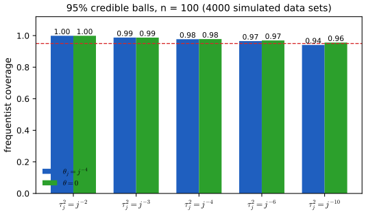
Figure 10.S11 (supplementary). Exercise 10.7(c)–(d): frequentist coverage of Bayesian 95% credible balls in the Normal means model with \(n=100\). Code: fig_s11,ex7_coverage. Download: PDF · SVG
Notes on the book
The book's website has no errata list. The points below are mine, each with the evidence.
Page 229: the SIMEX pseudo-errors need the factor \(\sigma_u\)
The text adds \(\sqrt\rho\,U_i\) with \(U_i\sim N(0,1)\) and then claims the limit (10.6). That limit needs \(\widetilde X_i=\Xb_i+\sqrt\rho\,\sigma_uU_i\), so that the total error variance is \((1+\rho)\sigma_u^2\) and \(\rho=-1\) corresponds to no error. With unit-variance pseudo-errors the limit is \(\beta_1\sigma_x^2/(\sigma_x^2+\sigma_u^2+\rho)\), confirmed by simulation (Filling the gap 10.2), and extrapolating to \(\rho=-1\) would target \(\beta_1\sigma_x^2/(\sigma_x^2+\sigma_u^2-1)\) instead of \(\beta_1\).
Page 231, (10.12)–(10.13): the weights depend on all the covariates
The expansion treats \(\ell_i\) as a function of \(\Xb_i\) alone. For a normalised smoother such as Nadaraya–Watson every weight depends on every covariate, and the second-order term must include all \(\partial^2/\partial X_i^2\) derivatives of the estimator. Read literally, (10.13) gives a correction that does not vanish when \(r\) is constant: in the design of Exercise 10.5 with \(r\equiv1\) it reaches 0.65, against exactly 0 for the full version, although no smoother is biased for a constant. The full version is in Filling the gap 10.4.
Page 233, (10.23): the second moment of \(K\) should be squared
The bias of a kernel density estimator is \(\tfrac12h^2\sigma_K^2f''\), so the integrated squared bias is \(\tfrac14h^4(\int y^2K)^2\int(f'')^2\). The exact risk confirms the square: 1.88 against 1.90 with it and 0.32 without (Filling the gap 10.6). The same page writes \(\hf_Y(y)\) for the estimator of \(f\); the subscript has no meaning here.
Page 233: the small-\(\sigma_u\) density correction has \(h^3\), not \(h\)
The correction is \(\frac{\sigma_u^2}{2}\hf_n''(x)=\frac{\sigma_u^2}{2nh^3}\sum_jK''((\Xb_j-x)/h)\); the book prints \(2nh\), which makes the correction \(h^2\) times too small, and sums over \(i\) a term indexed by \(j\). Numerically, the printed version removes only 16% of the bias in the example of Filling the gap 10.7, the corrected one 99%.
Page 238: the description of pool-adjacent-violators
The text always joins from \(P_0\) ("replace these two segments with one line segment joining \(P_0\) and \(P_2\) ... \(P_0\) and \(P_3\)"), which is only the special case in which every violation propagates back to the start. In general a violation is between two adjacent blocks anywhere, and merging can cascade backwards: with \(Y=(1,3,4,0)\) the last point pools with 4, then with 3, giving \((1,7/3,7/3,7/3)\), while the first block stays at 1. The stack algorithm of Filling the gap 10.14 handles this.
Page 239: cones
A cone is a set closed under multiplication by nonnegative scalars; the sets in question (monotone, positive, convex functions) are convex cones, closed also under addition. Closure under addition alone does not define a cone (Filling the gap 10.17).
Exercise 6 (p. 241): the integrand is missing \(r(s)\)
The model should read \(Y_i=\int K_i(s)r(s)\,\d s+\sigma\epsilon_i\), as in (10.25); as printed, \(Y_i\) does not depend on \(r\). Note also that the unnormalised kernels have mass \(b\sqrt\pi\), which for \(b=0.01\) shrinks the signal by a factor 56 (solution). Two typographical slips: "far to large" (p. 235) should be "far too large", and Section 10.5 has "to choose" for "choose".
Demonstrations for this chapter
Each demonstration runs in the browser, with seeded random numbers, and links back to these notes. The ▶ Demo boxes above open them already set to the case under discussion.
| Demonstration | What you can see | Sections and results |
|---|---|---|
| SIMEX and attenuation bias | Simulated errors-in-variables data: the naive slope, the method of moments, and SIMEX with quadratic and rational extrapolants, as the measurement error, \(n\) and \(B\) change. Presets: 1 Figure 10.2; 2 small error; 3 large error; 4 small sample; 5 few pseudo-data sets. | 10.1; Filling the gaps 10.1, 10.2 |
| Deconvolving a density | Naive, deconvolving and small-\(\sigma\) kernel estimates for Normal, Laplace and Cauchy errors, one or two bumps, \(n\) up to 10000, with exact MISE curves. Presets: 1 Exercise 4(b); 2 two bumps; 3 Laplace error; 4 Exercise 4(c); 5 too small a bandwidth. | 10.1; Filling the gaps 10.5–10.7, Exercise 10.4 |
| Isotonic regression and pool-adjacent-violators | Step through PAV point by point next to the cumulative sum diagram and its convex minorant, for five monotone functions, with the \(n^{-1/3}\) reference rate. Presets: 1 Figure 10.S9; 2 stepping; 3 a jump; 4 a flat function; 5 more data. | 10.8; Filling the gaps 10.14, 10.15 |
The Python code that produces every figure of this page is code/ch10_other_topics.py (see the code index).
References
- Wasserman, L. (2006). All of Nonparametric Statistics. Springer, New York. Chapter 10, pp. 227–242. www.stat.cmu.edu/~larry/all-of-nonpar.
- Barron, A., Schervish, M. J. and Wasserman, L. (1999). The consistency of posterior distributions in nonparametric problems. Annals of Statistics, 27, 536–561.
- Bickel, P. J., Klaassen, C. A. J., Ritov, Y. and Wellner, J. A. (1993). Efficient and Adaptive Estimation for Semiparametric Models. Johns Hopkins University Press.
- Brunk, H. D. (1970). Estimation of isotonic regression. In Nonparametric Techniques in Statistical Inference, Cambridge University Press, 177–195.
- Carroll, R. J., Ruppert, D. and Stefanski, L. A. (1995). Measurement Error in Nonlinear Models. Chapman and Hall.
- Chu, C.-K. and Marron, J. S. (1991). Comparison of two bandwidth selectors with dependent errors. Annals of Statistics, 19, 1906–1918.
- Cook, J. R. and Stefanski, L. A. (1994). Simulation-extrapolation estimation in parametric measurement error models. Journal of the American Statistical Association, 89, 1314–1328.
- Delaigle, A. and Hall, P. (2008). Using SIMEX for smoothing-parameter choice in errors-in-variables problems. Journal of the American Statistical Association, 103, 280–287.
- Diaconis, P. and Freedman, D. (1986). On the consistency of Bayes estimates. Annals of Statistics, 14, 1–26.
- Dümbgen, L. and Spokoiny, V. G. (2001). Multiscale testing of qualitative hypotheses. Annals of Statistics, 29, 124–152.
- Fan, J. (1991). On the optimal rates of convergence for nonparametric deconvolution problems. Annals of Statistics, 19, 1257–1272.
- Fan, J. and Marron, J. S. (1994). Fast implementations of nonparametric curve estimators. Journal of Computational and Graphical Statistics, 3, 35–56.
- Fan, J. and Truong, Y. K. (1993). Nonparametric regression with errors in variables. Annals of Statistics, 21, 1900–1925.
- Ferguson, T. S. (1973). A Bayesian analysis of some nonparametric problems. Annals of Statistics, 1, 209–230.
- Freedman, D. (1999). On the Bernstein–von Mises theorem with infinite-dimensional parameters. Annals of Statistics, 27, 1119–1140.
- Ghosal, S., Ghosh, J. K. and van der Vaart, A. W. (2000). Convergence rates of posterior distributions. Annals of Statistics, 28, 500–531.
- Ghosh, J. K. and Ramamoorthi, R. V. (2003). Bayesian Nonparametrics. Springer.
- Hall, P. and Wand, M. P. (1996). On the accuracy of binned kernel density estimators. Journal of Multivariate Analysis, 56, 165–184.
- Ingster, Yu. I. and Suslina, I. A. (2003). Nonparametric Goodness-of-Fit Testing under Gaussian Models. Springer.
- Knapik, B. T., van der Vaart, A. W. and van Zanten, J. H. (2011). Bayesian inverse problems with Gaussian priors. Annals of Statistics, 39, 2626–2657.
- Loader, C. (1999). Local Regression and Likelihood. Springer.
- Opsomer, J., Wang, Y. and Yang, Y. (2001). Nonparametric regression with correlated errors. Statistical Science, 16, 134–153.
- O'Sullivan, F. (1986). A statistical perspective on ill-posed inverse problems. Statistical Science, 1, 502–527.
- Robertson, T., Wright, F. T. and Dykstra, R. L. (1988). Order Restricted Statistical Inference. Wiley.
- Robinson, P. M. (1988). Root-N-consistent semiparametric regression. Econometrica, 56, 931–954.
- Sethuraman, J. (1994). A constructive definition of Dirichlet priors. Statistica Sinica, 4, 639–650.
- Speckman, P. (1988). Kernel smoothing in partial linear models. Journal of the Royal Statistical Society B, 50, 413–436.
- Stefanski, L. A. (1990). Rates of convergence of some estimators in a class of deconvolution problems. Statistics and Probability Letters, 9, 229–235.
- Stefanski, L. A. and Carroll, R. J. (1990). Deconvoluting kernel density estimators. Statistics, 21, 169–184.
- Staudenmayer, J. and Ruppert, D. (2004). Local polynomial regression and simulation-extrapolation. Journal of the Royal Statistical Society B, 66, 17–30.
- van der Vaart, A. W. (1998). Asymptotic Statistics. Cambridge University Press.
- van de Geer, S. (2000). Empirical Processes in M-Estimation. Cambridge University Press.
- Zhang, C.-H. (2002). Risk bounds in isotonic regression. Annals of Statistics, 30, 528–555.
The numerical statements in the text (the SIMEX limits, the excess bias, the second-order correction, the deconvolution identity and exact risks, the kernel constants, the ridge shortcut, the semiparametric and cross-validation simulations, the classification bound, the sieve risk, the isotonic fits and rate, the testing bounds and the coverage table) were confirmed numerically.