Sampling Methods
When an integral over a posterior distribution cannot be done exactly, we can draw random samples from the distribution and average over them. This chapter builds the samplers: transformations of uniform numbers, rejection and importance sampling, and then Markov chains (Metropolis-Hastings, Gibbs, slice sampling and hybrid Monte Carlo) whose long-run distribution is the one we want. Every proof that the book sketches or leaves to the reader is written out below.
Ch. 1 Introduction Ch. 2 Probability distributions Ch. 3 Linear regression Ch. 4 Linear classification Ch. 5 Neural networks Ch. 6 Kernel methods Ch. 7 Sparse kernel machines Ch. 8 Graphical models Ch. 9 Mixture models and EM Ch. 10 Approximate inference Ch. 11 Sampling methods Ch. 12 Continuous latent variables Ch. 13 Sequential data Ch. 14 Combining models
How to read these notes
They follow the book. Sections carry Bishop's numbers (11.1, 11.1.2, ...) and every displayed equation that appears in the book carries the book's own equation number, e.g. (11.14), so you can read these notes next to the book. Equations without a number are steps that the book skips.
Filling the gaps. Wherever the book says that a result "can be shown", "is easily seen" or is left as an exercise, an orange Filling the gap box gives the full argument. Proofs and derivations start hidden: open one with its bar, or use the button below.
Figures and demonstrations. Every numerical figure of the chapter is reproduced from scratch by the Python code, with real samplers, and the ▶ Demo boxes open an interactive demonstration already set to the case being discussed. Gaussian and gamma identities are proved once in the mathematical toolkit.
Main reference
C. M. Bishop, Pattern Recognition and Machine Learning, Springer (2006), Chapter 11, pages 523–558. Section, equation, figure and exercise numbers below refer to this book. Further reading is listed in the references.
The explanations, derivations and code are my own; equations are cited by their numbers in the book.
The chapter at a glance
- Introduction. An average of \(L\) independent draws estimates an expectation without bias, with variance \(\var[f]/L\) whatever the dimension (Result 11.1). Correlated draws inflate the variance by the integrated autocorrelation time (Result 11.2).
- 11.1 Exact samplers built from uniform numbers: the inverse distribution function, changes of variables (Box-Muller, Cholesky), rejection sampling (accept a proposal with probability \(\widetilde p/kq\)) and its adaptive version for log-concave densities. Importance sampling reweights proposals instead of discarding them; its weak point is the variance of the weights, measured by the effective sample size. Sampling-importance-resampling turns weighted samples into (approximately) unweighted ones; Monte Carlo EM and data augmentation use samples inside EM.
- 11.2 Markov chain Monte Carlo: design a Markov chain whose invariant distribution is \(p\) (detailed balance is the usual tool) and which forgets its start (ergodicity, proved for finite chains in Result 11.17). The Metropolis-Hastings acceptance probability makes any proposal satisfy detailed balance. Random-walk proposals need about \((\sigma_{\max}/\sigma_{\min})^2\) steps per independent sample.
- 11.3–11.4 Gibbs sampling updates one variable from its full conditional (a Metropolis-Hastings step that is always accepted); over-relaxation and blocking reduce its random walk. Slice sampling samples uniformly under the graph of \(\widetilde p\) and adapts its step size automatically.
- 11.5 Hybrid (Hamiltonian) Monte Carlo adds momentum variables and follows Hamiltonian dynamics, which conserves energy and phase-space volume; the leapfrog integrator keeps volume and reversibility exactly, and a Metropolis test corrects its energy error.
- 11.6 Ratios of normalising constants (model evidences) by importance sampling, and chaining through intermediate distributions.
Notation. The target density is \(p(\mathbf{z})=\widetilde p(\mathbf{z})/Z_p\), where \(\widetilde p\) can be evaluated and \(Z_p=\int\widetilde p(\mathbf{z})\,\d\mathbf{z}\) usually cannot. A proposal (or sampling) density is \(q\). Samples are \(\mathbf{z}^{(1)},\dots,\mathbf{z}^{(L)}\). For Markov chains, \(T(\mathbf{z},\mathbf{z}')\) is the probability (or density) of moving from \(\mathbf{z}\) to \(\mathbf{z}'\), and \(\tau\) counts steps. "Density" means density with respect to Lebesgue measure for continuous variables and probability mass for discrete ones; sums and integrals are interchangeable throughout.
Prerequisites. Change of variables in integrals (the Jacobian), the multivariate Gaussian and its conditionals (Section 2.3; toolkit), the gamma distribution (toolkit), EM (Chapter 9), and directed and undirected graphical models (Chapter 8) for the remarks on ancestral sampling and Markov blankets.
Printings. The text used here is a corrected printing. Where Bishop's errata list corrects an equation of this chapter, the notes give the corrected form and a short Erratum note naming the original.
Monte Carlo estimates
pp. 523–526 Most of what we want from a posterior distribution is an expectation: a posterior mean, a predictive probability, a posterior probability of a set. So the basic problem of the chapter is to compute
\[ \E[f]=\int f(\mathbf{z})\,p(\mathbf{z})\,\d\mathbf{z} \tag{11.1} \]for a function \(f\) and a distribution \(p\) (a sum replaces the integral for discrete \(\mathbf{z}\)), when the integral cannot be done analytically. The idea of Monte Carlo is to replace the distribution by a sample: if \(\mathbf{z}^{(1)},\dots,\mathbf{z}^{(L)}\) are drawn independently from \(p\), use
\[ \widehat f=\frac1L\sum_{l=1}^{L} f(\mathbf{z}^{(l)}) . \tag{11.2} \]Result 11.1 (the Monte Carlo estimator; Exercise 11.1) p. 524, (11.2)–(11.3)
Let \(\mathbf{z}^{(1)},\dots,\mathbf{z}^{(L)}\) be independent draws from \(p\) and let \(f\) have \(\E[f^2]\lt\infty\). Then
\[ \E[\widehat f]=\E[f],\qquad \var[\widehat f]=\frac1L\,\E\big[(f-\E[f])^2\big]=\frac{\var[f]}{L}. \tag{11.3} \]Moreover \(\widehat f\to\E[f]\) with probability one as \(L\to\infty\) (strong law of large numbers), and \(\sqrt L(\widehat f-\E[f])\) is approximately \(\N(0,\var[f])\) for large \(L\) (central limit theorem). Neither statement involves the dimension of \(\mathbf{z}\).
Proof
Write \(f_l=f(\mathbf{z}^{(l)})\). Each \(f_l\) has the distribution of \(f(\mathbf{z})\) with \(\mathbf{z}\sim p\), so \(\E[f_l]=\E[f]\) and \(\var[f_l]=\var[f]\).
Mean. Expectation is linear: \(\E[\widehat f]\)
Variance. Let \(g_l=f_l-\E[f]\), so \(\E[g_l]=0\) and \(\widehat f-\E[f]=\frac1L\sum_l g_l\). Then
\[ \var[\widehat f]=\E\Big[\Big(\frac1L\sum_{l}g_l\Big)^2\Big]=\frac1{L^2}\sum_{l=1}^{L}\sum_{m=1}^{L}\E[g_lg_m]. \]For \(l\ne m\), independence gives \(\E[g_lg_m]=\E[g_l]\,\E[g_m]=0\). Only the \(L\) diagonal terms survive, each equal to \(\E[g_l^2]=\E[(f-\E[f])^2]\), so \(\var[\widehat f]\)
Dimension. \(\var[f]\) is a property of the scalar random variable \(f(\mathbf{z})\); the dimension of \(\mathbf{z}\) enters only through it. So the standard error \(\sqrt{\var[f]/L}\) falls like \(L^{-1/2}\) in any dimension, whereas a grid with \(m\) points per axis needs \(m^D\) evaluations. Ten or twenty independent draws give a rough estimate (standard error about a quarter to a third of the standard deviation of \(f\)), which is the sense of the book's remark on p. 524. The limit theorems are the classical ones for independent, identically distributed \(f_l\) with finite mean (strong law) and finite variance (central limit theorem). ∎
The book adds two warnings p. 524. First, the samplers of Section 11.2 produce dependent draws, and then (11.3) no longer holds. Second, if \(f\) is large where \(p\) is small (Figure 11.1), \(\var[f]\) is large and so is the required \(L\). The next result quantifies the first warning; it is the reason why "effective sample size" appears throughout the chapter.
Result 11.2 (correlated samples and the effective sample size) p. 524
Let \(f_1,f_2,\dots\) be a stationary sequence (each \(f_l\) has the distribution of \(f(\mathbf{z})\), \(\mathbf{z}\sim p\)) with autocorrelations \(\rho_k=\mathrm{corr}(f_l,f_{l+k})\). Then \(\widehat f=\frac1L\sum_{l=1}^L f_l\) is still unbiased, and
\[ \var[\widehat f]=\frac{\var[f]}{L}\Big[1+2\sum_{k=1}^{L-1}\Big(1-\frac kL\Big)\rho_k\Big]\;\approx\;\frac{\var[f]}{L}\,\tau_{\rm int},\qquad \tau_{\rm int}=1+2\sum_{k=1}^{\infty}\rho_k, \]for large \(L\) when \(\sum_k|\rho_k|\lt\infty\). So \(L\) correlated draws are worth \(L_{\rm eff}=L/\tau_{\rm int}\) independent ones. For an autoregressive sequence with \(\rho_k=\phi^k\), \(\tau_{\rm int}=(1+\phi)/(1-\phi)\), which is about \(2/(1-\phi)\) when \(\phi\) is close to 1.
Proof
Unbiasedness was shown above without independence. With \(g_l=f_l-\E[f]\) and stationarity, \(\E[g_lg_m]=\var[f]\,\rho_{|l-m|}\). In the double sum \(\sum_{l,m}\E[g_lg_m]\) the lag \(k=|l-m|\) occurs \(L\) times for \(k=0\) and \(2(L-k)\) times for \(1\le k\le L-1\) (ordered pairs with \(m=l\pm k\)). Hence
\[ \var[\widehat f]=\frac{\var[f]}{L^2}\Big[L+2\sum_{k=1}^{L-1}(L-k)\rho_k\Big], \]which is the formula. If \(\sum_k|\rho_k|\lt\infty\), then \(\sum_{k\lt L}(1-k/L)\rho_k\to\sum_{k\ge1}\rho_k\) by dominated convergence (each term converges and is bounded by \(|\rho_k|\)). For \(\rho_k=\phi^k\) with \(|\phi|\lt1\): \(1+2\sum_{k\ge1}\phi^k\)
Negative correlations give \(\tau_{\rm int}\lt1\): antithetic schemes such as over-relaxation (Section 11.3) can beat independent sampling for some functions. Thinning (keeping every \(M\)th draw, as suggested on p. 538) makes the kept draws nearly independent, but it never reduces the variance of the estimate from a fixed run; it only saves storage.
Ancestral and logic sampling pp. 524–525, (11.4)
For a directed graphical model the joint distribution factorises as
\[ p(\mathbf{z})=\prod_{i=1}^{M}p(\mathbf{z}_i\given \mathrm{pa}_i). \tag{11.4} \]Ancestral sampling visits the nodes in an order in which parents come before children and draws each \(\mathbf{z}_i\) from \(p(\mathbf{z}_i\given\mathrm{pa}_i)\) with the parents set to their sampled values. The probability of producing \(\mathbf{z}\) is the product of the factors drawn, that is (11.4) itself, so one pass gives an exact draw from the joint. Logic sampling (Henrion, 1988) deals with observed nodes by sampling them too and throwing the whole draw away if a sampled value disagrees with the observation.
Filling the gap 11.1: logic sampling is exact, and how often it succeeds p. 525
The book argues informally that logic sampling "samples correctly from the posterior" and that its acceptance probability falls quickly. Both statements in one line each.
Derivation
Split the variables into hidden \(\mathbf{h}\) and observed \(\mathbf{x}\), with observed value \(\mathbf{x}_0\) (discrete). A complete ancestral pass yields \((\mathbf{h},\mathbf{x})\) with probability \(p(\mathbf{h},\mathbf{x})\), and the draw is kept iff \(\mathbf{x}=\mathbf{x}_0\). Stopping early as soon as one observed node disagrees does not change which draws are kept. So
\[ \Pr(\text{kept})=\sum_{\mathbf{h}}p(\mathbf{h},\mathbf{x}_0)=p(\mathbf{x}_0),\qquad \Pr(\mathbf{h}\given\text{kept})=\frac{p(\mathbf{h},\mathbf{x}_0)}{p(\mathbf{x}_0)}=p(\mathbf{h}\given\mathbf{x}_0). \]The kept draws are exact posterior draws, and the expected number of passes per kept draw is \(1/p(\mathbf{x}_0)\) (a geometric number of trials). The evidence \(p(\mathbf{x}_0)\) is a probability of a joint event over all observed nodes: with \(n\) observed nodes, each with \(K\) roughly comparable states, it is typically of order \(K^{-n}\), which is the exponential decay the book describes. ∎
For undirected graphs there is no ordering that makes one pass exact; Gibbs sampling (Section 11.3) is used instead. To sample a marginal \(p(\mathbf{u})\) from a joint sampler for \(p(\mathbf{u},\mathbf{v})\), simply ignore \(\mathbf{v}\) p. 525: the \(\mathbf{u}\)-component of a draw from the joint has the marginal distribution by definition.
11.1 Basic sampling algorithms
p. 526 We assume a supply of independent numbers uniform on \((0,1)\). (In practice these are pseudo-random numbers: a deterministic sequence that passes statistical tests of randomness. Their construction is outside the scope of the book and of these notes.) Everything in Section 11.1 transforms, filters or reweights such numbers.
11.1.1 Standard distributions
pp. 526–528 If \(z\) is uniform on \((0,1)\) and \(y=f(z)\) for a smooth monotone \(f\), the density of \(y\) is
\[ p(y)=p(z)\left|\frac{\d z}{\d y}\right| , \tag{11.5} \]with \(p(z)=1\) on \((0,1)\). We want to choose \(f\) so that \(y\) has a prescribed density \(p(y)\). Integrating (11.5) suggests
\[ z=h(y)\equiv\int_{-\infty}^{y}p(\widehat y)\,\d\widehat y , \tag{11.6} \]the distribution function of \(y\), and \(y=h^{-1}(z)\) (Figure 11.2).
Erratum. Some printings omit the absolute value in (11.5). It is needed when \(f\) is decreasing.
Result 11.3 (the inverse distribution function method; Exercise 11.2) p. 526, (11.5)–(11.6)
Let \(h\) be a distribution function on \(\R\) and define its generalised inverse \(h^{-}(z)=\inf\{y:h(y)\ge z\}\) for \(z\in(0,1)\). If \(z\) is uniform on \((0,1)\), then \(y=h^{-}(z)\) has distribution function \(h\). When \(h\) is continuous and strictly increasing on an interval, \(h^{-}=h^{-1}\) and \(y\) has density \(p(y)=h'(y)\).
Proof
The key equivalence. For \(z\in(0,1)\) and \(a\in\R\): \(h^{-}(z)\le a\iff z\le h(a)\). Indeed, if \(z\le h(a)\), then \(a\) belongs to the set \(\{y:h(y)\ge z\}\), so its infimum is at most \(a\). Conversely, distribution functions are right-continuous and nondecreasing, so the set \(\{y:h(y)\ge z\}\) is a closed half-line \([h^-(z),\infty)\); if \(h^{-}(z)\le a\), then \(a\) is in that half-line and \(h(a)\ge z\).
Conclusion. \(\Pr(y\le a)\)
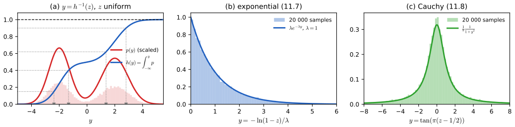
fig11_2. Download: PDF · SVGFilling the gap 11.2: the exponential and Cauchy examples pp. 526–527, (11.7)–(11.8); Exercise 11.3
The book gives the exponential transformation and says the Cauchy one is expressed with the tangent. Both in full.
Derivation
Exponential. For
\[ p(y)=\lambda\exp(-\lambda y),\qquad 0\le y\lt\infty, \tag{11.7} \]the lower limit in (11.6) is 0 (the density vanishes below it), and \(h(y)\)
Cauchy. For
\[ p(y)=\frac1\pi\,\frac{1}{1+y^2}, \tag{11.8} \]\(h(y)\)
Equivalently: if \(\theta\) is uniform on \((-\pi/2,\pi/2)\), then \(\tan\theta\) is standard Cauchy, since \(|\d\theta/\d y|\)
Several variables p. 527. If \(\mathbf{y}=\mathbf{f}(\mathbf{z})\) is a smooth bijection between open sets of \(\R^M\), then
\[ p(y_1,\dots,y_M)=p(z_1,\dots,z_M)\left|\frac{\partial(z_1,\dots,z_M)}{\partial(y_1,\dots,y_M)}\right| , \tag{11.9} \]where the last factor is the absolute value of the determinant of the matrix of partial derivatives \(\partial z_i/\partial y_j\) (the Jacobian of the inverse map).
Filling the gap 11.3: why the Jacobian appears in (11.9) p. 527, (11.9)
Derivation
Let \(\mathbf{g}=\mathbf{f}^{-1}\), so \(\mathbf{z}=\mathbf{g}(\mathbf{y})\). For any set \(B\) in the \(\mathbf{y}\) space, \(\mathbf{y}\in B\) exactly when \(\mathbf{z}\in\mathbf{g}(B)\), so
\[ \Pr(\mathbf{y}\in B)=\int_{\mathbf{g}(B)}p_{\mathbf{z}}(\mathbf{z})\,\d\mathbf{z}=\int_{B}p_{\mathbf{z}}(\mathbf{g}(\mathbf{y}))\,\big|\det \mathbf{J}_{\mathbf{g}}(\mathbf{y})\big|\,\d\mathbf{y}, \]by the change-of-variables theorem for multiple integrals (substitute \(\mathbf{z}=\mathbf{g}(\mathbf{y})\); a small box of volume \(\d\mathbf{y}\) is mapped to a parallelepiped of volume \(|\det\mathbf{J}_{\mathbf{g}}|\,\d\mathbf{y}\), with \((\mathbf{J}_{\mathbf{g}})_{ij}\)
The Box-Muller method pp. 527–528, (11.10)–(11.12)
Draw \(z_1,z_2\) uniform on \((-1,1)\) (from \(z\mapsto2z-1\)) and keep the pair only if \(z_1^2+z_2^2\le1\). The kept pairs are uniform on the unit disc, with density \(1/\pi\) (Figure 11.3). With \(r^2=z_1^2+z_2^2\), set
\[ y_1=z_1\left(\frac{-2\ln r^2}{r^2}\right)^{1/2}, \tag{11.10} \] \[ y_2=z_2\left(\frac{-2\ln r^2}{r^2}\right)^{1/2}. \tag{11.11} \]Then
\[ p(y_1,y_2)=p(z_1,z_2)\left|\frac{\partial(z_1,z_2)}{\partial(y_1,y_2)}\right|=\left[\frac{1}{\sqrt{2\pi}}\exp(-y_1^2/2)\right]\left[\frac{1}{\sqrt{2\pi}}\exp(-y_2^2/2)\right], \tag{11.12} \]so \(y_1\) and \(y_2\) are independent standard Gaussians.
Erratum. Some printings have \(\ln z_1\) and \(\ln z_2\) in the numerators of (11.10) and (11.11); both should be \(\ln r^2\), as above.
Result 11.4 (Box-Muller, polar form; Exercise 11.4) p. 528, (11.10)–(11.12)
(a) The kept pairs \((z_1,z_2)\) are uniform on the unit disc, and a pair is kept with probability \(\pi/4\approx0.785\).
(b) The map (11.10)–(11.11) is a bijection from the punctured disc \(0\lt r^2\lt1\) onto \(\R^2\setminus\{\mathbf{0}\}\), with Jacobian determinant \(\partial(y_1,y_2)/\partial(z_1,z_2)=-2/r^2\).
(c) Hence (11.12) holds: \(y_1,y_2\) are independent \(\N(0,1)\).
(d) Equivalently (the trigonometric form of Box and Muller, 1958): if \(u_1,u_2\) are independent uniforms on \((0,1)\), then \(\sqrt{-2\ln u_1}\cos(2\pi u_2)\) and \(\sqrt{-2\ln u_1}\sin(2\pi u_2)\) are independent \(\N(0,1)\).
Proof
(a) \((z_1,z_2)\) is uniform on the square \((-1,1)^2\) of area 4. Conditioning a uniform distribution on a subset gives the uniform distribution on that subset, so the kept pairs are uniform on the disc of area \(\pi\), with density \(1/\pi\); the probability of keeping a pair is the ratio of areas, \(\pi/4\). (This is rejection sampling with a uniform proposal, Section 11.1.2.)
(b) Write \(s=r^2=z_1^2+z_2^2\) and \(g(s)=\sqrt{-2\ln s/s}\), so \(y_i=z_i\,g(s)\). The map keeps the direction of \((z_1,z_2)\) and sends the radius \(r\) to \(\rho=r\,g(r^2)=\sqrt{-2\ln r^2}\), which decreases strictly from \(+\infty\) (as \(r\to0\)) to \(0\) (as \(r\to1\)). Hence each ray of the punctured disc is mapped one-to-one onto the corresponding open ray of the plane, and the map is a bijection onto \(\R^2\setminus\{\mathbf 0\}\). For the Jacobian, \(\partial s/\partial z_j=2z_j\), so
\[ \frac{\partial y_i}{\partial z_j}=\delta_{ij}\,g(s)+2z_iz_j\,g'(s),\qquad\text{i.e.}\qquad \mathbf{J}=g\,\mathbf{I}+2g'\,\mathbf{z}\mathbf{z}^\T . \]The matrix \(\mathbf{z}\mathbf{z}^\T\) has eigenvalue \(s\) (eigenvector \(\mathbf{z}\)) and \(0\) (the perpendicular direction), so \(\mathbf{J}\) has eigenvalues \(g+2sg'\) and \(g\), and \(\det\mathbf{J}=g\,(g+2sg')\). Now \(\ln g=\tfrac12\ln(-2\ln s)-\tfrac12\ln s\), so
\[ \frac{g'}{g}=\frac12\cdot\frac{-2/s}{-2\ln s}-\frac{1}{2s}=\frac{1}{2s\ln s}-\frac1{2s},\qquad g+2sg'=g\Big(1+\frac{1}{\ln s}-1\Big)=\frac{g}{\ln s}. \]Therefore \(\det\mathbf{J}=g^2/\ln s\)
(c) By (11.9) with the inverse Jacobian \(|\partial(z_1,z_2)/\partial(y_1,y_2)|\)
which factorises as (11.12). The single point \(\mathbf{y}=\mathbf 0\) and the null event \(s=0\) do not matter.
(d) In polar coordinates the uniform point on the disc has \(s=r^2\) uniform on \((0,1)\) (because \(\Pr(r^2\le t)=\pi t/\pi=t\)) and angle \(\theta\) uniform on \((0,2\pi)\), independent of \(s\). The output has radius \(\sqrt{-2\ln s}\) and the same angle. Replacing \((s,\theta)\) by \((u_1,2\pi u_2)\) gives the trigonometric form. As a by-product, \(y_1^2+y_2^2=-2\ln s\) is exponential with mean 2, the \(\chi^2_2\) distribution, as it must be. The polar form avoids evaluating sine and cosine at the price of rejecting \(1-\pi/4\approx21\%\) of the pairs (Marsaglia and Bray, 1964). ∎
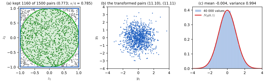
fig11_3. Download: PDF · SVGCorrelated Gaussians p. 528. If \(y\sim\N(0,1)\), then \(\sigma y+\mu\sim\N(\mu,\sigma^2)\). For a vector with mean \(\bm\mu\) and covariance \(\bm\Sigma\), factorise \(\bm\Sigma=\mathbf{L}\mathbf{L}^\T\) with \(\mathbf{L}\) lower triangular (the Cholesky decomposition) and use \(\mathbf{y}=\bm\mu+\mathbf{L}\mathbf{z}\) with \(\mathbf{z}\) a vector of independent standard Gaussians.
Result 11.5 (sampling a multivariate Gaussian; Exercise 11.5) p. 528
Let \(\mathbf{z}\sim\N(\mathbf 0,\mathbf{I}_D)\), let \(\bm\Sigma\) be symmetric positive definite and let \(\mathbf{A}\) be any \(D\times D\) matrix with \(\mathbf{A}\mathbf{A}^\T=\bm\Sigma\) (for example the Cholesky factor \(\mathbf{L}\)). Then \(\mathbf{y}\)
Proof
Moments. \(\E[\mathbf{y}]\)
Gaussianity. \(\mathbf{A}\) is invertible because \(\det(\mathbf{A})^2=\det\bm\Sigma\gt0\). The inverse map is \(\mathbf{z}=\mathbf{A}^{-1}(\mathbf{y}-\bm\mu)\) with constant Jacobian determinant \(\det\mathbf{A}^{-1}\), so by (11.9)
\[ p(\mathbf{y})=\frac{1}{(2\pi)^{D/2}}\exp\Big\{-\tfrac12(\mathbf{y}-\bm\mu)^\T\mathbf{A}^{-\T}\mathbf{A}^{-1}(\mathbf{y}-\bm\mu)\Big\}\frac{1}{|\det\mathbf{A}|}=\N(\mathbf{y}\given\bm\mu,\bm\Sigma), \]since \(\mathbf{A}^{-\T}\mathbf{A}^{-1}\)
The transformation method needs a distribution function that can be computed and inverted, which is rare. The next two techniques need much less: the ability to evaluate \(\widetilde p\) and to sample a simpler \(q\) p. 528.
11.1.2 Rejection sampling
pp. 528–530 Suppose we can evaluate
\[ p(z)=\frac{1}{Z_p}\,\widetilde p(z) \tag{11.13} \]up to the unknown constant \(Z_p\), and can sample a proposal density \(q(z)\). Choose a constant \(k\) with \(kq(z)\ge\widetilde p(z)\) for all \(z\); the function \(kq\) is the comparison function or envelope (Figure 11.4).
Algorithm 11.1 (rejection sampling) p. 529
- Draw \(z_0\sim q\).
- Draw \(u_0\) uniform on \([0,kq(z_0)]\).
- If \(u_0\le\widetilde p(z_0)\), accept \(z_0\) as a draw from \(p\); otherwise reject it and return to step 1.
Steps 2 and 3 together accept \(z_0\) with probability \(\widetilde p(z_0)/kq(z_0)\); one usually draws \(v\) uniform on \((0,1)\) and accepts if \(v\,kq(z_0)\le\widetilde p(z_0)\).
Result 11.6 (uniform under the graph) p. 529
Let \(g\ge0\) be integrable with \(\int g\gt0\), and let \(A_g=\{(z,u):0\le u\le g(z)\}\) be the region under its graph. Then a pair \((z,u)\) is uniform on \(A_g\) if and only if \(z\) has density \(g/\int g\) and, given \(z\), \(u\) is uniform on \([0,g(z)]\).
Proof
The area of \(A_g\) is \(\int g(z)\,\d z\), so the uniform density on \(A_g\) is \(\mathbb{1}\{0\le u\le g(z)\}/\int g\). Integrating out \(u\) gives the marginal \(g(z)/\int g\); dividing the joint by this marginal gives the conditional \(\mathbb 1\{0\le u\le g(z)\}/g(z)\), the uniform density on \([0,g(z)]\). Conversely, multiplying that marginal and that conditional gives back the uniform joint density. ∎
Result 11.7 (rejection sampling is exact; Exercise 11.6) p. 529, (11.14)
Assume \(kq(z)\ge\widetilde p(z)\) for all \(z\). Then (a) a proposal \(z_0\) is accepted with probability \(\widetilde p(z_0)/kq(z_0)\); (b) the overall acceptance probability is
\[ p(\text{accept})=\int\Big\{\frac{\widetilde p(z)}{kq(z)}\Big\}q(z)\,\d z=\frac1k\int\widetilde p(z)\,\d z=\frac{Z_p}{k}; \tag{11.14} \](c) an accepted value has density \(p\); (d) the number of proposals needed per accepted value is geometric with mean \(k/Z_p\), and successive accepted values are independent.
Proof
(a) Given \(z_0\), \(u_0\) is uniform on \([0,kq(z_0)]\) and \(0\le\widetilde p(z_0)\le kq(z_0)\), so \(\Pr(u_0\le\widetilde p(z_0)\given z_0)\)
(b) Average (a) over \(z_0\sim q\): the factors \(q\) cancel, which is (11.14).
(c) By the product rule, the joint density of "propose \(z\) and accept it" is \(q(z)\,\widetilde p(z)/kq(z)\)
Geometrically: \((z_0,u_0)\) is uniform under the graph of \(kq\) (Result 11.6 with \(g=kq\)); conditioning on the subset \(A_{\widetilde p}\) leaves it uniform there, and then Result 11.6 with \(g=\widetilde p\) says that \(z_0\) has density \(p\).
(d) Attempts are independent and each succeeds with probability \(Z_p/k\), so the number of attempts is geometric with that success probability and mean \(k/Z_p\). Because each attempt uses fresh random numbers, the accepted value of one round is independent of the others. ∎
So the waste is the fraction of the area under \(kq\) that is not under \(\widetilde p\), and \(k\) should be as small as the condition \(kq\ge\widetilde p\) allows: \(k^\star=\sup_z\widetilde p(z)/q(z)\). If \(p\) has heavier tails than \(q\), the ratio is unbounded and no \(k\) exists.
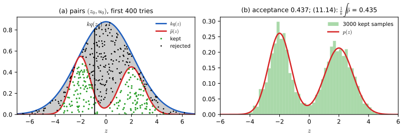
fig11_4. Download: PDF · SVGErratum. In some printings the label of the lower curve of Figure 11.4 (and of Figure 11.13) is \(p\); it should be \(\widetilde p\).
The gamma distribution with a Cauchy envelope pp. 529–530, (11.15)–(11.16)
The gamma density
\[ \Gam(z\given a,b)=\frac{b^a z^{a-1}\exp(-bz)}{\Gamma(a)} \tag{11.15} \]is bell-shaped for \(a\gt1\), with mode \((a-1)/b\) (toolkit). A Cauchy density is also bell-shaped, easy to sample by the transformation method, and has heavier tails than the gamma, so a scaled Cauchy can serve as an envelope:
\[ q(z)=\frac{k}{1+(z-c)^2/b^2}, \tag{11.16} \]which is generated by \(z=b\tan y+c\) with \(y\) uniform on \((-\pi/2,\pi/2)\) (Exercise 11.7). The book states that the rejection rate is smallest for \(c=a-1\), \(b^2=2a-1\), with \(k\) as small as possible. Here the letter \(b\) in (11.16) is the Cauchy scale; for these formulas to make sense the gamma must have rate 1, and we take \(b=1\) in (11.15) for this example (a general rate only rescales \(z\)). The book's Figure 11.5 uses \(a=10\).
Filling the gap 11.4: where \(c=a-1\), \(b^2=2a-1\) and the optimal \(k\) come from p. 530, (11.16)
The book gives the values without derivation. We show that with the envelope centred at the mode and touching the gamma there, \(b^2=2a-1\) is exactly the smallest Cauchy scale that keeps the envelope above the gamma everywhere, compute \(k\) and the acceptance rate, and check numerically how far this is from the best possible Cauchy envelope.
Derivation
Setting. Target \(p(z)=\Gam(z\given a,1)\), \(a\gt1\), with mode \(m=a-1\). Write \(s\) for the Cauchy scale (the book's \(b\) in (11.16)) to avoid a clash, and \(g(z)=1/(1+(z-c)^2/s^2)\), so the envelope is \(kg\). The smallest valid \(k\) for given \((c,s)\) is \(k(c,s)=\sup_{z\gt0}p(z)/g(z)\), and since \(\int kg\,\d z=k\pi s\), the acceptance probability (11.14) is \(1/(k\pi s)\).
Centre the envelope at the mode. Take \(c=m\) and ask the envelope to touch the gamma at its mode, \(k=p(m)\). Then \(kg\ge p\) everywhere iff \(\varphi(z)\le0\) for all \(z\gt0\), where
\[ \varphi(z)=\ln p(z)-\ln p(m)+\ln\Big(1+\frac{(z-m)^2}{s^2}\Big)=(a-1)\ln\frac zm-(z-m)+\ln\Big(1+\frac{(z-m)^2}{s^2}\Big). \]With \(t=z-m\) and using \((a-1)/z-1=(m-z)/z=-t/z\),
\[ \varphi'(z)=-\frac tz+\frac{2t}{s^2+t^2}=\frac{t\,\{2z-s^2-t^2\}}{z\,(s^2+t^2)}=\frac{t\,\{-t^2+2t+(2a-2-s^2)\}}{z\,(s^2+t^2)}, \]using \(2z=2m+2t=2a-2+2t\). If \(s^2\ge2a-1\), the quadratic \(-t^2+2t+(2a-2-s^2)\)
The optimal constant. In the book's parametrisation (11.16), where \(q\) already includes \(k\),
\[ k=\Gam(a-1\given a,1)=\frac{(a-1)^{a-1}e^{-(a-1)}}{\Gamma(a)},\qquad p(\text{accept})=\frac{1}{k\pi\sqrt{2a-1}}=\frac{\Gamma(a)\,e^{a-1}}{\pi\,(a-1)^{a-1}\sqrt{2a-1}} . \]For \(a=10\): \(k=0.13176\) (the peak height in Figure 11.5) and the acceptance probability is \(0.554\). By Stirling's formula, \(\Gamma(a)\)
Is it the best Cauchy envelope? Not quite. Minimising the area \(k(c,s)\pi s\) over both \(c\) and \(s\) numerically (my computation: a fine grid for the supremum, Nelder–Mead for \((c,s)\)) gives, for \(a=10\), \(c\approx9.33\), \(s^2\approx9.55\) and acceptance \(0.646\); for \(a=3\), \(0.615\) instead of \(0.526\). The optimal envelope is narrower, centred slightly right of the mode, and taller than the gamma's peak. So the book's "minimum reject rate" holds within the family of envelopes centred at the mode with the mode's height; the advantage of that family is the closed form above. ∎
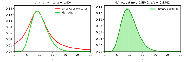
fig11_5. Download: PDF · SVG11.1.3 Adaptive rejection sampling
pp. 530–532 Finding a tight envelope by hand is often hard. Gilks and Wild (1992) build it automatically when \(p\) is log-concave, that is, when \(\ell(z)=\ln\widetilde p(z)\) is concave (for differentiable \(\ell\): \(\ell'\) is nonincreasing). Many densities met in Gibbs sampling are log-concave: Gaussian, gamma with shape \(\ge1\), beta with both parameters \(\ge1\), logistic regression posteriors, and products of these.
Result 11.8 (tangent envelopes of a log-concave density; Exercise 11.8) pp. 530–531, (11.17)
Let \(\ell=\ln\widetilde p\) be concave and differentiable, and let \(z_1\lt z_2\lt\dots\lt z_n\) be grid points with \(\ell'(z_1)\gt0\gt\ell'(z_n)\). Let \(t_i(z)=\ell(z_i)+\ell'(z_i)(z-z_i)\) be the tangent at \(z_i\), and \(u(z)=\min_i t_i(z)\). Then
(a) \(u(z)\ge\ell(z)\) for all \(z\), with equality at the grid points, so \(e^{u}\ge\widetilde p\) is an envelope;
(b) \(u=t_i\) on the interval \(\widehat z_{i-1,i}\lt z\le\widehat z_{i,i+1}\), where \(\widehat z_{i,i+1}\) is the intersection of the tangents at \(z_i\) and \(z_{i+1}\) (with \(\widehat z_{0,1}=-\infty\), \(\widehat z_{n,n+1}=+\infty\)):
(c) the normalised envelope is the piecewise exponential density
\[ q(z)=k_i\lambda_i\exp\{-\lambda_i(z-z_i)\},\qquad \widehat z_{i-1,i}\lt z\le\widehat z_{i,i+1}, \tag{11.17} \]with \(\lambda_i=-\ell'(z_i)\) (so the tangent at \(z_i\) has slope \(-\lambda_i\)) and \(k_i=\widetilde p(z_i)/(\lambda_iC)\), where
\[ C=\sum_{i=1}^{n}\frac{\widetilde p(z_i)}{\lambda_i}\Big[e^{-\lambda_i(\widehat z_{i-1,i}-z_i)}-e^{-\lambda_i(\widehat z_{i,i+1}-z_i)}\Big] \]is the area under \(e^{u}\) (a term with \(\lambda_i=0\) is read as its limit \(\widetilde p(z_i)(\widehat z_{i,i+1}-\widehat z_{i-1,i})\)). Equivalently, the \(k_i\) are fixed by continuity of \(q\) at the intersection points and by \(\int q=1\).
Proof
(a) A differentiable concave function lies below each of its tangents: for concave \(\ell\) and any \(z,z_i\), \(\ell(z)\le\ell(z_i)+\ell'(z_i)(z-z_i)\). (Proof: by concavity, for \(0\lt\theta\le1\), \(\ell(z_i+\theta(z-z_i))\)
(b) Because \(\ell'\) is nonincreasing, the slopes satisfy \(\ell'(z_1)\ge\ell'(z_2)\ge\dots\). Two lines with slopes \(\ell'(z_i)\gt\ell'(z_{i+1})\) cross once; to the left of the crossing the line with the larger slope is lower. So \(t_i\le t_{i+1}\) exactly for \(z\le\widehat z_{i,i+1}\), and the crossing points are ordered, \(\widehat z_{i-1,i}\le\widehat z_{i,i+1}\) (a standard property of the lower envelope of lines with decreasing slopes). Hence the minimum is \(t_i\) between consecutive crossing points. The formula for \(\widehat z_{i,i+1}\) is the solution of \(t_i(z)=t_{i+1}(z)\), a linear equation in \(z\). (If \(\ell'(z_i)=\ell'(z_{i+1})\), then \(\ell\) is linear between the points and either tangent can be used.)
(c) On piece \(i\), \(e^{t_i(z)}\)
Algorithm 11.2 (adaptive rejection sampling; Exercise 11.9) pp. 530–531
- Start with a few grid points on both sides of the mode (\(\ell'(z_1)\gt0\gt\ell'(z_n)\)); compute \(\ell\), \(\ell'\), the intersections \(\widehat z\) and the piece masses \(M_i=\int_{\text{piece }i}q\)
\({}=k_i\big[e^{-\lambda_i(\widehat z_{i-1,i}-z_i)}-e^{-\lambda_i(\widehat z_{i,i+1}-z_i)}\big]\), which sum to 1. - Choose a piece \(i\) with probability \(M_i\) (a discrete draw by Result 11.3).
- Sample within the piece by inverting its distribution function: with \(v\) uniform on \((0,1)\), \(a=\widehat z_{i-1,i}\) and \(b=\widehat z_{i,i+1}\), \[ z=a-\frac1{\lambda_i}\ln\Big[1-v\big(1-e^{-\lambda_i(b-a)}\big)\Big] \] (for the unbounded left piece, \(a=-\infty\) and \(\lambda_1\lt0\): \(z=b+|\lambda_1|^{-1}\ln v\); for the unbounded right piece, \(b=\infty\) and \(\lambda_n\gt0\): \(z=a-\lambda_n^{-1}\ln v\)).
- Accept \(z\) with probability \(\widetilde p(z)/e^{u(z)}\). If it is rejected, add \(z\) to the grid (the envelope tightens), and return to step 2.
Gilks and Wild also use a lower "squeeze" function (the chords between grid points, which lie below a concave \(\ell\)): if \(v\le\exp\{\text{chord}(z)-u(z)\}\) the draw is accepted without evaluating \(\widetilde p\).
Filling the gap 11.5: sampling the piecewise exponential, and why adapting the envelope is allowed pp. 530–531; Exercise 11.9
Derivation
Within a piece. On \([a,b]\) the density is proportional to \(e^{-\lambda(z-a)}\) (the factor \(e^{\lambda(z_i-a)}\) is a constant). Its distribution function is \(F(z)\)
Adaptation. The envelope used at a given attempt depends on the earlier rejected points, but conditionally on everything that happened before the attempt it is a fixed valid envelope, and Result 11.7 applied conditionally says that an accepted value has density \(p\) given the past. A value whose conditional distribution given the past is always \(p\) is independent of the past; hence the accepted values are independent draws from \(p\). Each rejection adds a grid point where the envelope was loose, so the expected acceptance probability increases towards 1. ∎
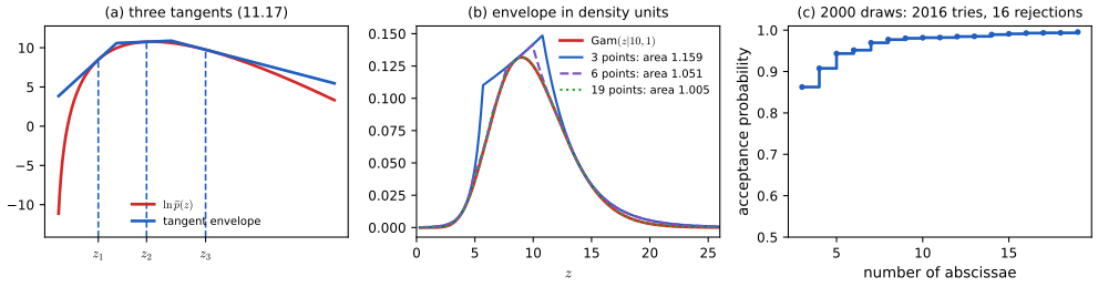
fig11_6. Download: PDF · SVGErratum. Some printings print the range in (11.17) and the following sentence incorrectly; the corrected form is the one above: the piece for \(z_i\) runs between \(\widehat z_{i-1,i}\) and \(\widehat z_{i,i+1}\), the intersections of the tangent at \(z_i\) with its neighbours.
Variants p. 531: a derivative-free version uses chords through pairs of grid points instead of tangents (Gilks, 1992), and adaptive rejection Metropolis sampling (Gilks, Best and Tan, 1995) handles densities that are not log-concave by following each rejection step with a Metropolis-Hastings step (Section 11.2.2).
Rejection sampling in high dimensions pp. 531–532
To see what dimension does to rejection sampling, the book samples \(p=\N(\mathbf 0,\sigma_p^2\mathbf I)\) in \(D\) dimensions using the proposal \(q=\N(\mathbf 0,\sigma_q^2\mathbf I)\), a nearly perfect proposal.
Result 11.9 (acceptance falls exponentially with dimension) p. 531
A finite \(k\) with \(kq\ge p\) exists iff \(\sigma_q\ge\sigma_p\). The smallest one is \(k=(\sigma_q/\sigma_p)^D\), and the acceptance probability is \(1/k=(\sigma_p/\sigma_q)^D\). For \(\sigma_q=1.01\,\sigma_p\) and \(D=1000\) it is \(1.01^{-1000}\approx4.8\times10^{-5}\), about 1 in 21 000.
Proof
The ratio of the two densities is
\[ \frac{p(\mathbf z)}{q(\mathbf z)}=\frac{(2\pi\sigma_p^2)^{-D/2}e^{-\lVert\mathbf z\rVert^2/2\sigma_p^2}}{(2\pi\sigma_q^2)^{-D/2}e^{-\lVert\mathbf z\rVert^2/2\sigma_q^2}}=\Big(\frac{\sigma_q}{\sigma_p}\Big)^D\exp\Big\{-\frac{\lVert\mathbf z\rVert^2}{2}\Big(\frac1{\sigma_p^2}-\frac1{\sigma_q^2}\Big)\Big\}. \]If \(\sigma_q\lt\sigma_p\), the exponent is positive and the ratio is unbounded as \(\lVert\mathbf z\rVert\to\infty\), so no \(k\) works. If \(\sigma_q\ge\sigma_p\), the exponent is \(\le0\) and the supremum, attained at \(\mathbf z=\mathbf 0\), is \((\sigma_q/\sigma_p)^D\). Both densities are normalised (\(Z_p=1\)), so by (11.14) the acceptance probability is \(1/k\). Numerically \(1000\ln1.01=9.950\), and \(e^{-9.950}=4.77\times10^{-5}=1/20\,959\), in line with the book's "approximately 1/20 000". The loss comes from the peak: in \(D\) dimensions, a 1% mismatch of scale is a factor \(1.01^D\) mismatch of height at the mode. ∎
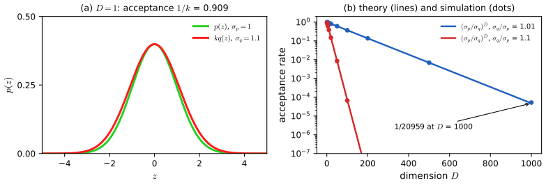
fig11_7. Download: PDF · SVGThe exponential loss is generic: an envelope must dominate \(\widetilde p\) everywhere, and in high dimensions any mismatch is multiplied across dimensions. Rejection sampling is useful in one or two dimensions and as a building block (for example inside Gibbs sampling) but not on its own in high dimensions p. 532.
11.1.4 Importance sampling
pp. 532–534 Importance sampling estimates expectations directly, without producing draws from \(p\). A grid approximation
\[ \E[f]\simeq\sum_{l=1}^{L}p(\mathbf z^{(l)})\,f(\mathbf z^{(l)}) \tag{11.18} \](times the volume of a grid cell, which the book absorbs) needs a number of points exponential in the dimension and wastes nearly all of them where \(p\) is negligible. Instead, draw \(\mathbf z^{(l)}\) from a proposal \(q\) and correct by the ratio \(p/q\):
\[ \E[f]=\int f(\mathbf z)p(\mathbf z)\,\d\mathbf z=\int f(\mathbf z)\frac{p(\mathbf z)}{q(\mathbf z)}q(\mathbf z)\,\d\mathbf z\simeq\frac1L\sum_{l=1}^{L}\frac{p(\mathbf z^{(l)})}{q(\mathbf z^{(l)})}f(\mathbf z^{(l)}). \tag{11.19} \]The \(r_l=p(\mathbf z^{(l)})/q(\mathbf z^{(l)})\) are the importance weights. All samples are kept.
Result 11.10 (importance sampling: unbiasedness and variance) pp. 532–533, (11.19)
Assume \(q(\mathbf z)\gt0\) wherever \(f(\mathbf z)p(\mathbf z)\ne0\). Then the estimator \(\widehat f_{\rm IS}\)
which may be infinite. The variance is smallest (over all \(q\)) for \(q^\star(\mathbf z)\)
Proof
Apply Result 11.1 to the function \(\mathbf z\mapsto f(\mathbf z)p(\mathbf z)/q(\mathbf z)\) under \(q\). Its mean is \(\int f\frac pq\,q=\int fp=\E[f]\) (this is where positivity of \(q\) is needed: on a set where \(q=0\) but \(fp\ne0\), the integral of \(fp\) would be missed). Its second moment is \(\int f^2\frac{p^2}{q^2}q=\int f^2p^2/q\), which gives the variance.
For the optimum, by the Cauchy–Schwarz inequality, for any \(q\),
\[ \Big(\int|f|p\Big)^2=\Big(\int\frac{|f|p}{\sqrt q}\sqrt q\Big)^2\le\int\frac{f^2p^2}{q}\int q=\int\frac{f^2p^2}{q}, \]with equality iff \(|f|p/\sqrt q\) is proportional to \(\sqrt q\), i.e. \(q\propto|f|p\). So the second moment is minimised by \(q^\star\), where it equals \((\E|f|)^2\); if \(f\ge0\), that is \(\E[f]^2\) and the variance is zero. The optimum needs \(\int|f|p\), the very kind of integral we are trying to compute, so it is a guide (put proposal mass where \(|f|p\) is large, as the book says on p. 532) rather than a recipe. ∎
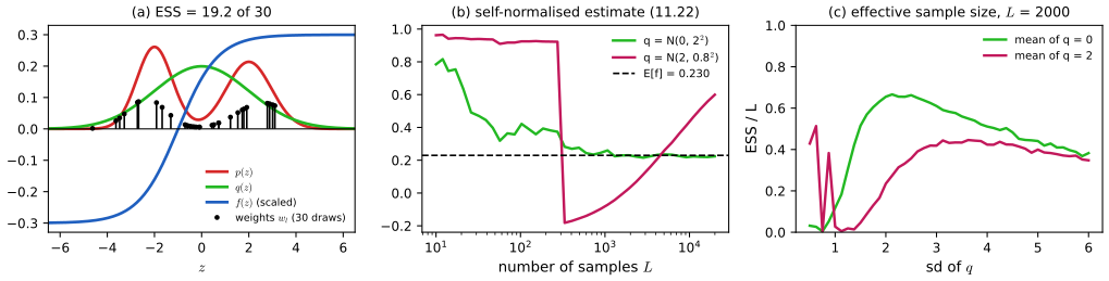
fig11_8. Download: PDF · SVGUnnormalised densities p. 533. Usually \(p=\widetilde p/Z_p\) with \(Z_p\) unknown, and perhaps \(q=\widetilde q/Z_q\) too. Then
\[ \E[f]=\int f(\mathbf z)p(\mathbf z)\,\d\mathbf z=\frac{Z_q}{Z_p}\int f(\mathbf z)\frac{\widetilde p(\mathbf z)}{\widetilde q(\mathbf z)}q(\mathbf z)\,\d\mathbf z\simeq\frac{Z_q}{Z_p}\,\frac1L\sum_{l=1}^{L}\widetilde r_lf(\mathbf z^{(l)}), \tag{11.20} \]with \(\widetilde r_l\)
and dividing (11.20) by (11.21) gives the self-normalised estimator
\[ \E[f]\simeq\sum_{l=1}^{L}w_lf(\mathbf z^{(l)}), \tag{11.22} \] \[ w_l=\frac{\widetilde r_l}{\sum_m\widetilde r_m}=\frac{\widetilde p(\mathbf z^{(l)})/q(\mathbf z^{(l)})}{\sum_m\widetilde p(\mathbf z^{(m)})/q(\mathbf z^{(m)})}. \tag{11.23} \]Result 11.11 (the self-normalised estimator) p. 533, (11.20)–(11.23)
Assume \(q\gt0\) wherever \(\widetilde p\gt0\) and \(\E_p|f|\lt\infty\). Then (a) \(\widehat f_{\rm SN}=\sum_lw_lf(\mathbf z^{(l)})\) converges to \(\E_p[f]\) with probability one; it needs neither \(Z_p\) nor \(Z_q\), and the weights \(w_l\) are the same whether \(q\) or \(\widetilde q\) is used. (b) It is biased for finite \(L\), with bias of order \(1/L\). (c) Writing \(w(\mathbf z)=p(\mathbf z)/q(\mathbf z)\) for the normalised weight function and \(\mu=\E_p[f]\), for large \(L\)
\[ \var[\widehat f_{\rm SN}]\approx\frac1L\,\E_q\big[w(\mathbf z)^2\{f(\mathbf z)-\mu\}^2\big]=\frac1L\,\E_p\big[w(\mathbf z)\{f(\mathbf z)-\mu\}^2\big]. \]Proof
(a) Write \(\widehat f_{\rm SN}=A_L/B_L\) with \(A_L\)
(b, c) Linearise the ratio around the limits (the delta method). With \(a=Z_p\mu\), \(b=Z_p\),
\[ \frac{A_L}{B_L}-\mu=\frac{A_L-\mu B_L}{B_L}=\frac{1}{b}(A_L-\mu B_L)\Big\{1-\frac{B_L-b}{b}+O_p(L^{-1})\Big\}. \]The leading term \((A_L-\mu B_L)/b\)
When importance sampling fails pp. 533–534
If \(p\,f\) puts much of its mass where \(q\) is small, a few weights dominate and the effective number of samples is far below \(L\). Worse, if no sample has landed there yet, the weights may look harmless and the estimate may still be badly wrong, "with no diagnostic indication" (p. 534). The cleanest way to see this is through the tails.
Filling the gap 11.6: light-tailed proposals give infinite variance pp. 533–534
The book warns that \(q\) "should not be small or zero in regions where \(p(\mathbf z)\) may be significant". Here is an exact calculation showing what goes wrong when \(q\) has lighter tails than \(p\), and a run that shows why the sample itself does not reveal it.
Derivation
Second moment of the weights. Take \(p=\N(0,\sigma_p^2)\) and \(q=\N(0,\sigma_q^2)\) in one dimension. Then
\[ \E_q[w^2]=\int\frac{p(z)^2}{q(z)}\,\d z=\frac{\sigma_q}{\sqrt{2\pi}\,\sigma_p^2}\int\exp\Big\{-z^2\Big(\frac1{\sigma_p^2}-\frac1{2\sigma_q^2}\Big)\Big\}\d z . \]The integral is finite iff \(1/\sigma_p^2\gt1/(2\sigma_q^2)\), i.e. \(\sigma_q^2\gt\sigma_p^2/2\), and then a Gaussian integral gives
\[ \E_q[w^2]=\frac{\sigma_q^2}{\sigma_p\sqrt{2\sigma_q^2-\sigma_p^2}}\qquad(\text{and }(\cdot)^D\text{ in }D\text{ independent dimensions}). \]It equals 1 at \(\sigma_q=\sigma_p\) and is larger otherwise (Jensen's inequality, below). For \(\sigma_q^2\le\sigma_p^2/2\) it is infinite, so the weights have infinite variance, and so does the estimator of \(\E[f]\) for \(f=1\) or \(f=z^2\). The estimator is still unbiased and consistent (the strong law needs only a finite mean), but it converges slower than \(L^{-1/2}\) and erratically. In \(D\) dimensions the finite value is raised to the power \(D\): even a well-matched proposal degrades exponentially, as rejection sampling did.
Why the sample does not warn you. The sample variance of \(L\) weights is always finite. Large weights come from the tails of \(p\) that \(q\) rarely visits; until one of those rare draws occurs, the weights look well behaved. When one does occur, it dominates the sum. My run (seed 0), estimating \(\E_p[z^2]=1\) for \(p=\N(0,1)\) with the self-normalised estimator:
| Proposal | \(L=10^3\) | \(L=10^4\) | \(L=10^5\) | \(L=10^6\) |
|---|---|---|---|---|
| \(q=\N(0,0.5^2)\) (light tails, \(\E_q[w^2]=\infty\)): estimate (ESS/\(L\)) | 1.304 (0.036) | 0.743 (0.147) | 0.999 (0.014) | 0.931 (0.015) |
| \(q=\N(0,2^2)\) (heavy tails, \(\E_q[w^2]=4/\sqrt7\)): estimate (ESS/\(L\)) | 0.979 (0.675) | 1.001 (0.659) | 0.995 (0.664) | 0.999 (0.662) |
With the light-tailed proposal the estimate wanders and the effective sample size (defined in the next box) jumps around, from 147 per 1000 draws down to 14 per 1000, rather than settling; with the heavy-tailed proposal it settles at \(\sqrt7/4=0.661\) per draw, exactly \(1/\E_q[w^2]\). Rule: choose \(q\) with tails at least as heavy as those of \(p\) (a Student \(t\) instead of a Gaussian, for example; see the toolkit), so that \(w=p/q\) is bounded. ∎
Result 11.12 (effective sample size) p. 534
Compared with \(L\) independent draws from \(p\), self-normalised importance sampling has variance inflated by approximately \(\E_q[w^2]=1+\var_q[w]\ge1\), so it is worth about
\[ L_{\rm eff}=\frac{L}{\E_q[w^2]}\quad\text{draws, estimated by}\quad \widehat L_{\rm eff}=\frac{\big(\sum_l\widetilde r_l\big)^2}{\sum_l\widetilde r_l^2}=\frac{1}{\sum_lw_l^2}, \]which lies between 1 (one weight carries everything) and \(L\) (equal weights).
Proof
The approximation (Kong, 1992; Kong, Liu and Wong, 1994). By Result 11.11c, the variance is about \(\frac1L\E_p[w(f-\mu)^2]\), while independent sampling from \(p\) gives \(\frac1L\E_p[(f-\mu)^2]\). Write \(\E_p[w(f-\mu)^2]\)
The estimate. Replace \(\E_q[w^2]\)
Importance sampling on graphical models p. 534, (11.24)
With evidence \(\mathbf x\) on some nodes of a directed graph, the target is the posterior of the other nodes, \(p(\mathbf z\given\mathbf x)\)
Filling the gap 11.7: the likelihood-weighting weight p. 534, (11.24)
Derivation
Ancestral sampling with the evidence nodes clamped produces a configuration \(\mathbf z\) (evidence nodes at their observed values) with probability \(q(\mathbf z)\)
11.1.5 Sampling-importance-resampling
pp. 534–536 Rejection sampling needs a constant \(k\), which may be unknown or so large that almost nothing is accepted. Sampling-importance-resampling (SIR; Rubin, 1987, 1988) avoids \(k\):
Algorithm 11.3 (sampling-importance-resampling) p. 535
- Draw \(\mathbf z^{(1)},\dots,\mathbf z^{(L)}\) independently from \(q\).
- Compute the normalised weights \(w_1,\dots,w_L\) of (11.23).
- Draw a second set of \(L\) values from the discrete distribution that puts probability \(w_l\) on \(\mathbf z^{(l)}\) (with replacement).
Result 11.13 (SIR is exact as \(L\to\infty\)) p. 535, (11.25)–(11.26)
Assume \(q\gt0\) wherever \(\widetilde p\gt0\). For a resampled value \(z^\ast\) (univariate case), conditionally on the first-stage sample,
\[ p(z^\ast\le a)=\sum_{l:\,z^{(l)}\le a}w_l=\frac{\sum_l I(z^{(l)}\le a)\,\widetilde p(z^{(l)})/q(z^{(l)})}{\sum_l\widetilde p(z^{(l)})/q(z^{(l)})}, \tag{11.25} \]and as \(L\to\infty\) this tends, with probability one and for every \(a\), to
\[ \frac{\int I(z\le a)\{\widetilde p(z)/q(z)\}q(z)\,\d z}{\int\{\widetilde p(z)/q(z)\}q(z)\,\d z}=\frac{\int I(z\le a)\widetilde p(z)\,\d z}{\int\widetilde p(z)\,\d z}=\int I(z\le a)\,p(z)\,\d z, \tag{11.26} \]the distribution function of \(p\). So the resampled values converge in distribution to \(p\). The same holds in several dimensions with \(I(\mathbf z\in B)\) for any set \(B\).
Proof
Given the first stage, the resampled value equals \(z^{(l)}\) with probability \(w_l\), so its distribution function is the sum of the weights of the points \(\le a\), which is (11.25) after inserting (11.23). Numerator and denominator divided by \(L\) are sample means of \(I(z\le a)\widetilde p/q\) and of \(\widetilde p/q\) under \(q\); both have finite means (\(\int I\,\widetilde p\le Z_p\) and \(Z_p\)), so by the strong law they converge almost surely to the integrals in (11.26), the denominator to \(Z_p\gt0\). The ratio converges to their ratio. Convergence of distribution functions at every \(a\) is convergence in distribution; unconditionally, \(\Pr(z^\ast\le a)\) is the expectation of (11.25), which converges too by bounded convergence (the ratio is between 0 and 1). For a fixed \(L\) the resampled values are only approximately from \(p\): their distribution is the self-normalised estimator of Result 11.11, with the same \(O(1/L)\) bias. If \(q=p\), all weights equal \(1/L\) and resampling returns draws from \(p\). ∎
For moments, resampling only adds noise: use the weighted original sample directly p. 536,
\[ \E[f(\mathbf z)]=\frac{\int f(\mathbf z)[\widetilde p(\mathbf z)/q(\mathbf z)]q(\mathbf z)\,\d\mathbf z}{\int[\widetilde p(\mathbf z)/q(\mathbf z)]q(\mathbf z)\,\d\mathbf z}\simeq\sum_{l=1}^{L}w_lf(\mathbf z^{(l)}). \tag{11.27} \](Given the first stage, the average of \(f\) over the resampled values has conditional mean \(\sum_lw_lf(\mathbf z^{(l)})\) and a positive conditional variance, so by the law of total variance it is never more precise than (11.27).) Resampling is useful when unweighted draws are needed, as in particle filters (Section 13.3.4).
Erratum. Some printings write \(\mathbf z_l\) in the last line of (11.27); it should be \(\mathbf z^{(l)}\).
11.1.6 Sampling and the EM algorithm
pp. 536–537 When the E step of EM (Chapter 9) cannot be done in closed form, it can be done by sampling. With hidden variables \(\mathbf Z\), data \(\mathbf X\) and parameters \(\bm\theta\), the M step maximises
\[ Q(\bm\theta,\bm\theta^{\rm old})=\int p(\mathbf Z\given\mathbf X,\bm\theta^{\rm old})\ln p(\mathbf Z,\mathbf X\given\bm\theta)\,\d\mathbf Z, \tag{11.28} \]and Monte Carlo EM (Wei and Tanner, 1990) replaces it by an average over draws \(\mathbf Z^{(l)}\) from \(p(\mathbf Z\given\mathbf X,\bm\theta^{\rm old})\):
\[ Q(\bm\theta,\bm\theta^{\rm old})\simeq\frac1L\sum_{l=1}^{L}\ln p(\mathbf Z^{(l)},\mathbf X\given\bm\theta). \tag{11.29} \]Filling the gap 11.8: what Monte Carlo EM keeps and loses, MAP, and stochastic EM p. 536, (11.28)–(11.29)
Derivation
Unbiased for each \(\bm\theta\). For fixed \(\bm\theta\), (11.29) is a Monte Carlo average of the function \(\mathbf Z\mapsto\ln p(\mathbf Z,\mathbf X\given\bm\theta)\) under \(p(\mathbf Z\given\mathbf X,\bm\theta^{\rm old})\), so by Result 11.1 it is unbiased for \(Q(\bm\theta,\bm\theta^{\rm old})\) with variance of order \(1/L\). The M step then maximises the random function \(\widehat Q\) "in the usual way": for exponential-family complete-data models it only needs the averages of the sufficient statistics over the \(L\) draws.
What is lost. EM's monotonicity (Chapter 9, Result 9.15) comes from \(Q(\bm\theta^{\rm new},\bm\theta^{\rm old})\)
MAP. The MAP version of EM maximises \(Q(\bm\theta,\bm\theta^{\rm old})\)
Stochastic EM (Celeux and Diebolt, 1985) is the case \(L=1\) for a finite mixture. The E step draws one label per point, \(\mathbf z_n\)
Data augmentation p. 537. For a full Bayesian treatment we want draws from \(p(\bm\theta\given\mathbf X)\) (or from the joint \(p(\bm\theta,\mathbf Z\given\mathbf X)\)), and suppose that the complete-data posterior \(p(\bm\theta\given\mathbf Z,\mathbf X)\) is easy to sample. The IP algorithm of Tanner and Wong (1987) alternates two steps, built on the identities
\[ p(\mathbf Z\given\mathbf X)=\int p(\mathbf Z\given\bm\theta,\mathbf X)\,p(\bm\theta\given\mathbf X)\,\d\bm\theta, \tag{11.30} \] \[ p(\bm\theta\given\mathbf X)=\int p(\bm\theta\given\mathbf Z,\mathbf X)\,p(\mathbf Z\given\mathbf X)\,\d\mathbf Z. \tag{11.31} \]Algorithm 11.4 (IP algorithm, data augmentation) p. 537, (11.30)–(11.32)
- I step (imputation). For \(l=1,\dots,L\): draw \(\bm\theta^{(l)}\) from the current approximation of \(p(\bm\theta\given\mathbf X)\), then \(\mathbf Z^{(l)}\)
\({}\sim p(\mathbf Z\given\bm\theta^{(l)},\mathbf X)\). - P step (posterior). Update the approximation to \[ p(\bm\theta\given\mathbf X)\simeq\frac1L\sum_{l=1}^{L}p(\bm\theta\given\mathbf Z^{(l)},\mathbf X), \tag{11.32} \] a mixture that is easy to sample: pick \(l\) uniformly, then draw from \(p(\bm\theta\given\mathbf Z^{(l)},\mathbf X)\).
Result 11.14 (why the IP algorithm works) p. 537
Let \(K(\bm\theta',\bm\theta)\)
Proof
The map. The I step draws \(\bm\theta'\sim g\) and \(\mathbf Z\)
(a) If \(g=p(\cdot\given\mathbf X)\), the I-step density of \(\mathbf Z\) is \(p(\mathbf Z\given\mathbf X)\) by (11.30), and then the P step returns \(p(\bm\theta\given\mathbf X)\) by (11.31). The two identities are the sum rule applied to the joint \(p(\bm\theta,\mathbf Z\given\mathbf X)\), factorised by the product rule in the two possible orders.
(b) By Bayes' rule, \(p(\mathbf Z\given\bm\theta',\mathbf X)p(\bm\theta'\given\mathbf X)\)
which is symmetric in \(\bm\theta\) and \(\bm\theta'\): this is detailed balance (11.40), and it implies (a) again (Result 11.16 below).
(c) With \(\pi=p(\cdot\given\mathbf X)\) and (a), \(g_{\rm new}-\pi\)
(d) With \(L=1\), the P step's "mixture" is the single density \(p(\bm\theta\given\mathbf Z^{(1)},\mathbf X)\), and the next I step draws \(\bm\theta\) from it and then \(\mathbf Z\) given \(\bm\theta\): alternately drawing \(\bm\theta\given\mathbf Z\) and \(\mathbf Z\given\bm\theta\) from their full conditionals is Gibbs sampling. ∎
The distinction between parameters and hidden variables is artificial here p. 537; from now on the problem is simply to sample a given distribution \(p(\mathbf z)\).
11.2 Markov chain Monte Carlo
pp. 537–539 Rejection and importance sampling degrade exponentially with dimension because a single fixed proposal must cover the whole of \(p\). Markov chain Monte Carlo (MCMC) instead lets the proposal depend on the current state: from \(\mathbf z^{(\tau)}\) it proposes a candidate \(\mathbf z^\star\)
In the Metropolis algorithm the proposal is symmetric, \(q(\mathbf z_A\given\mathbf z_B)\)
Algorithm 11.5 (Metropolis; Metropolis-Hastings with \(q_k\) and (11.44)) pp. 538, 541
- Start from some \(\mathbf z^{(1)}\) with \(\widetilde p(\mathbf z^{(1)})\gt0\).
- For \(\tau=1,2,\dots\): draw \(\mathbf z^\star\)
\({}\sim q(\mathbf z\given\mathbf z^{(\tau)})\) and \(u\) uniform on \((0,1)\). - If \(u\lt A(\mathbf z^\star,\mathbf z^{(\tau)})\), set \(\mathbf z^{(\tau+1)}=\mathbf z^\star\); otherwise set \(\mathbf z^{(\tau+1)}=\mathbf z^{(\tau)}\) (the current state is repeated in the output).
A move uphill (\(\widetilde p(\mathbf z^\star)\)
Repeating the current state after a rejection is essential: dropping repeats would over-represent the states that are easy to leave. The draws are dependent, so Result 11.2 applies; the book suggests keeping every \(M\)th draw, which gives nearly independent draws but, as noted there, does not make estimates from a given run more precise.
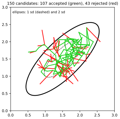
fig11_9. Download: PDF · SVGRandom walks p. 539. To see why local moves are slow, take the random walk on the integers with
\[ p(z^{(\tau+1)}=z^{(\tau)})=0.5, \tag{11.34} \] \[ p(z^{(\tau+1)}=z^{(\tau)}+1)=0.25, \tag{11.35} \] \[ p(z^{(\tau+1)}=z^{(\tau)}-1)=0.25, \tag{11.36} \]started at \(z^{(0)}=0\).
Erratum. Some printings say \(z^{(1)}=0\) after (11.36); the walk starts at \(z^{(0)}=0\).
Result 11.15 (random walks travel like \(\sqrt\tau\); Exercise 11.10) p. 539
For the walk (11.34)–(11.36), \(\E[z^{(\tau)}]=0\) and \(\E[(z^{(\tau)})^2]=\E[(z^{(\tau-1)})^2]+\tfrac12\), so \(\E[(z^{(\tau)})^2]=\tau/2\): the root-mean-square distance travelled after \(\tau\) steps is \(\sqrt{\tau/2}\).
Proof
Write \(z^{(\tau)}=z^{(\tau-1)}+\xi_\tau\), where the step \(\xi_\tau\in\{-1,0,1\}\) has probabilities \(0.25,0.5,0.25\) and is independent of the past. Then \(\E[\xi_\tau]=0\) and \(\E[\xi_\tau^2]=0.25+0.25=\tfrac12\). By induction \(\E[z^{(\tau)}]=\E[z^{(\tau-1)}]=\dots=0\). Squaring, \(\E[(z^{(\tau)})^2]\)
This square-root law is the central inefficiency of MCMC with local proposals, and avoiding it motivates over-relaxation (Section 11.3) and hybrid Monte Carlo (Section 11.5).
11.2.1 Markov chains
pp. 539–541 We now make precise when a Markov chain "converges to \(p\)".
Definition 11.1 (Markov chain, homogeneity, invariance, detailed balance) pp. 539–540, (11.37)–(11.40)
(a) A sequence \(\mathbf z^{(1)},\mathbf z^{(2)},\dots\) is a (first-order) Markov chain if
\[ p(\mathbf z^{(m+1)}\given\mathbf z^{(1)},\dots,\mathbf z^{(m)})=p(\mathbf z^{(m+1)}\given\mathbf z^{(m)}). \tag{11.37} \]It is specified by an initial distribution and the transition probabilities \(T_m(\mathbf z^{(m)},\mathbf z^{(m+1)})\)
(b) A distribution \(p^\star\) is invariant (stationary) for \(T\) if one step leaves it unchanged:
\[ p^\star(\mathbf z)=\sum_{\mathbf z'}T(\mathbf z',\mathbf z)\,p^\star(\mathbf z'). \tag{11.39} \](c) \(T\) satisfies detailed balance with respect to \(p^\star\) (the chain is reversible) if
\[ p^\star(\mathbf z)\,T(\mathbf z,\mathbf z')=p^\star(\mathbf z')\,T(\mathbf z',\mathbf z)\quad\text{for all }\mathbf z,\mathbf z'. \tag{11.40} \]For continuous states, sums become integrals and \(T(\mathbf z,\cdot)\) is a probability distribution that may contain a point mass at \(\mathbf z\) (a rejected move); (11.40) is then read as equality of the measures \(p^\star(\d\mathbf z)T(\mathbf z,\d\mathbf z')\) and \(p^\star(\d\mathbf z')T(\mathbf z',\d\mathbf z)\).
In words, (11.38) says that the probability of being at \(\mathbf z\) next is the probability of being at each \(\mathbf z'\) now times the probability of moving from there to \(\mathbf z\), summed over \(\mathbf z'\). Detailed balance says more: in equilibrium the probability flow from \(\mathbf z\) to \(\mathbf z'\) equals the flow back, for each pair separately. Equivalently, if \(\mathbf z^{(m)}\sim p^\star\), the pair \((\mathbf z^{(m)},\mathbf z^{(m+1)})\) has the same joint distribution as \((\mathbf z^{(m+1)},\mathbf z^{(m)})\): a film of the stationary chain looks the same run backwards, hence "reversible".
Result 11.16 (detailed balance implies invariance) p. 540, (11.41)
If \(T\) satisfies detailed balance (11.40) with respect to \(p^\star\), then \(p^\star\) is invariant for \(T\):
\[ \sum_{\mathbf z'}p^\star(\mathbf z')T(\mathbf z',\mathbf z)=\sum_{\mathbf z'}p^\star(\mathbf z)T(\mathbf z,\mathbf z')=p^\star(\mathbf z)\sum_{\mathbf z'}p(\mathbf z'\given\mathbf z)=p^\star(\mathbf z). \tag{11.41} \]The converse fails: invariance does not imply detailed balance.
Proof
The first equality replaces each term by the other side of (11.40); the second takes \(p^\star(\mathbf z)\) out of the sum; the third uses that the transition probabilities out of \(\mathbf z\) sum to one. In the continuous case, integrate both sides of (11.40) over \(\mathbf z'\) in the same way.
The converse fails. On three states, let the chain move deterministically \(1\to2\to3\to1\). The uniform distribution is invariant (each state receives exactly the mass of its predecessor), but \(p^\star(1)T(1,2)=\tfrac13\ne0=p^\star(2)T(2,1)\). A chain can circulate in equilibrium; detailed balance forbids net circulation. So detailed balance is sufficient but not necessary, as the book says. ∎
Ergodicity p. 540. Invariance is not enough: the identity transition leaves every distribution invariant and never moves. We also need the chain to forget its starting point: \(p(\mathbf z^{(m)})\to p^\star\) as \(m\to\infty\) for every initial distribution. Such a chain is ergodic, and \(p^\star\) is then its unique equilibrium distribution. Even detailed balance plus "can reach every state" is not enough: the two-state chain that always switches state satisfies detailed balance with respect to \((\tfrac12,\tfrac12)\), but started in state 1 it is in state 1 at every even step, so \(p(\mathbf z^{(m)})\) oscillates and never converges (periodicity). The book quotes Neal (1993) for "weak restrictions" that suffice; for finite state spaces a complete proof is short.
Result 11.17 (convergence of finite Markov chains) p. 540
Let the state space be finite, let \(T\) be a transition matrix, and suppose some power \(T^m\) has all entries positive (equivalently, for a finite chain: \(T\) is irreducible and aperiodic). Let \(\beta\)
(a) \(T\) has exactly one invariant distribution \(p^\star\);
(b) for every initial distribution \(\mu\), with \(\mu_n\) the distribution after \(n\) steps,
(c) (ergodic theorem) for every function \(f\) and every starting state, \(\frac1L\sum_{l=1}^{L}f(\mathbf z^{(l)})\)
Proof
Treat distributions as row vectors, so one step maps \(\mu\) to \(\mu T\) (this is (11.38)), and write \(\lVert d\rVert_1=\sum|d(\mathbf z)|\).
Step 1 (contraction). Let \(P=T^m\) and \(c(\mathbf z')\)
The braces are \(\ge0\) and, summed over \(\mathbf z'\), equal \(1-\beta\). Hence
\[ \lVert dP\rVert_1\le\sum_{\mathbf z'}\sum_{\mathbf z}|d(\mathbf z)|\big\{P(\mathbf z,\mathbf z')-c(\mathbf z')\big\}=(1-\beta)\lVert d\rVert_1 . \]The same argument with \(c\equiv0\) shows \(\lVert dT\rVert_1\le\lVert d\rVert_1\): one step of any chain never increases the distance between two distributions.
Step 2 (existence and uniqueness). The set of distributions is closed and bounded in \(\R^{|S|}\), hence complete, and \(\mu\mapsto\mu P\) is a contraction on it (factor \(1-\beta\lt1\)). By the Banach fixed-point theorem it has a unique fixed point \(\pi\). Then \(\pi T\) is also fixed by \(P\), since \((\pi T)P=(\pi P)T=\pi T\); by uniqueness \(\pi T=\pi\), so \(\pi\) is invariant for \(T\). Any invariant distribution of \(T\) is invariant for \(P\), so equals \(\pi\). Call it \(p^\star\). (In MCMC we know \(p^\star\) in advance; the point of (a) is that there is no other.)
Step 3 (convergence). Write \(n=km+j\) with \(0\le j\lt m\). Since \(p^\star=p^\star T^n\), \(\lVert\mu T^n-p^\star\rVert_1\)
Step 4 (ergodic theorem, sketch). Fix a state \(\mathbf a\). By the Markov property the chain restarts afresh at each visit to \(\mathbf a\), so the excursions between successive visits are independent and identically distributed; they have finite mean length because the geometric convergence of Step 3 makes long excursions exponentially unlikely. Applying the strong law of large numbers to the sums of \(f\) over excursions and to their lengths gives the limit \(\E[\text{sum of }f\text{ over an excursion}]/\E[\text{length}]\), and the same identity applied to the indicator of each state shows that this ratio is \(\E_{p^\star}[f]\). (Full details: Levin, Peres and Wilmer, 2017, Chapter 4.)
Positive power. For a finite chain, "some \(T^m\gt0\) entrywise" is equivalent to irreducibility (every state can reach every other) plus aperiodicity (the return times to a state have greatest common divisor 1); the number-theoretic argument is in Levin, Peres and Wilmer (2017), Proposition 1.7. ∎
General state spaces. For continuous \(\mathbf z\) the corresponding theorem (Tierney, 1994, Theorem 1) reads: if \(T\) has invariant distribution \(p^\star\), is \(p^\star\)-irreducible (from any start, every set of positive \(p^\star\)-probability is reached with positive probability) and aperiodic, then \(p(\mathbf z^{(m)})\to p^\star\) in total variation for \(p^\star\)-almost every starting point, and ergodic averages converge to \(\E_{p^\star}[f]\) for every \(f\) with \(\E_{p^\star}|f|\lt\infty\). These are the "weak restrictions" of the book. In practice: build \(T\) with \(p\) invariant (usually through detailed balance), and check that the chain can get from anywhere to anywhere.
Combining transitions pp. 540–541. Samplers are usually assembled from base transitions \(B_1,\dots,B_K\), either as a mixture (pick \(B_k\) with probability \(\alpha_k\))
\[ T(\mathbf z',\mathbf z)=\sum_{k=1}^{K}\alpha_kB_k(\mathbf z',\mathbf z),\qquad\alpha_k\ge0,\ \sum_k\alpha_k=1, \tag{11.42} \]or as a composition (apply \(B_1\), then \(B_2\), ..., then \(B_K\))
\[ T(\mathbf z',\mathbf z)=\sum_{\mathbf z_1}\dots\sum_{\mathbf z_{K-1}}B_1(\mathbf z',\mathbf z_1)\dots B_{K-1}(\mathbf z_{K-2},\mathbf z_{K-1})B_K(\mathbf z_{K-1},\mathbf z). \tag{11.43} \]Erratum. In some printings the last sum in (11.43) runs over \(\mathbf z_{n-1}\); it should be \(\mathbf z_{K-1}\).
Result 11.18 (mixtures and compositions of transitions) p. 541
Suppose \(p^\star\) is invariant for each \(B_k\). Then (a) \(p^\star\) is invariant for the mixture (11.42) and for the composition (11.43). (b) If each \(B_k\) satisfies detailed balance with respect to \(p^\star\), so does the mixture; (c) the composition need not; (d) the symmetric composition \(B_1,B_2,\dots,B_K,B_K,\dots,B_2,B_1\) does.
Proof
Use matrix notation on a finite space (the general case is identical with integrals): \(p^\star\) is a row vector, invariance reads \(p^\star B=p^\star\), and with \(\mathbf D=\diag(p^\star)\) detailed balance reads \(\mathbf DB=B^\T\mathbf D\) (entry \((\mathbf z,\mathbf z')\) of both sides is (11.40)).
(a) Mixture: \(p^\star T\)
(b) \(\mathbf DT\)
(c) For \(T=B_1B_2\): \(\mathbf DB_1B_2\)
(d) For \(S=B_1\cdots B_KB_K\cdots B_1\), move \(\mathbf D\) from left to right through all \(2K\) factors, each time using \(\mathbf DB_k=B_k^\T\mathbf D\):
\[ \mathbf DS=B_1^\T\cdots B_K^\T B_K^\T\cdots B_1^\T\,\mathbf D=(B_1\cdots B_KB_K\cdots B_1)^\T\mathbf D=S^\T\mathbf D, \]because the transpose of a product is the product of the transposes in reverse order, and the palindromic order is its own reverse. ∎
The typical use: each \(B_k\) changes only a subset of the variables (a "coordinate" move). A single \(B_k\) is then not ergodic, but the mixture or composition can be.
11.2.2 The Metropolis-Hastings algorithm
pp. 541–542 Hastings (1970) allowed asymmetric proposals. From the current state \(\mathbf z^{(\tau)}\), draw \(\mathbf z^\star\)
where \(k\) labels one of several available transition types (to be mixed or composed as in (11.42)–(11.43)). The unknown \(Z_p\) cancels, and for a symmetric proposal the \(q\) factors cancel too, giving (11.33). The extra factor corrects for a proposal that goes more easily one way than the other.
Result 11.19 (Metropolis-Hastings satisfies detailed balance) p. 541, (11.45)
The Metropolis-Hastings transition with proposal \(q_k\) and acceptance (11.44) satisfies detailed balance with respect to \(p\), and therefore leaves \(p\) invariant. Off the diagonal,
\[ \begin{aligned} p(\mathbf z)q_k(\mathbf z'\given\mathbf z)A_k(\mathbf z',\mathbf z)&=\min\big(p(\mathbf z)q_k(\mathbf z'\given\mathbf z),\,p(\mathbf z')q_k(\mathbf z\given\mathbf z')\big)\\ &=\min\big(p(\mathbf z')q_k(\mathbf z\given\mathbf z'),\,p(\mathbf z)q_k(\mathbf z'\given\mathbf z)\big)\\ &=p(\mathbf z')q_k(\mathbf z\given\mathbf z')A_k(\mathbf z,\mathbf z'). \end{aligned} \tag{11.45} \]Proof
The transition. From \(\mathbf z\), the chain moves to \(\mathbf z'\ne\mathbf z\) with density \(q_k(\mathbf z'\given\mathbf z)A_k(\mathbf z',\mathbf z)\) (propose it, then accept it), and stays at \(\mathbf z\) with the remaining probability \(r(\mathbf z)\)
Off-diagonal part. Multiply \(A_k(\mathbf z',\mathbf z)=\min(1,R)\), with \(R\)
Diagonal part. The point mass contributes \(p(\mathbf z)r(\mathbf z)\) on the diagonal \(\mathbf z'=\mathbf z\) to both \(p(\d\mathbf z)T(\mathbf z,\d\mathbf z')\) and its mirror image, so it is symmetric automatically. Detailed balance holds, and invariance follows from Result 11.16.
Metropolis. If \(q_k(\mathbf a\given\mathbf b)\)
Ergodicity. If \(q_k(\mathbf z'\given\mathbf z)\gt0\) for all \(\mathbf z,\mathbf z'\) (the book's sufficient condition, p. 538), then from any \(\mathbf z\) every set \(B\) with \(p(B)\gt0\) has \(T(\mathbf z,B)\ge\int_Bq_kA_k\gt0\) in one step, which gives irreducibility and aperiodicity, and Tierney's theorem applies. ∎
Erratum. Some printings have a different (incorrect) form of (11.45) and write \(\mathbf z^\tau\) for \(\mathbf z^{(\tau)}\) just before (11.44); the corrected forms are given above.
Other acceptance functions also give detailed balance (for example Barker's \(R/(1+R)\)), but \(\min(1,R)\) accepts as often as possible and, by Peskun's (1973) theorem, gives estimates with the smallest asymptotic variance among them for the same proposal.
Choosing the proposal scale pp. 541–542
With a Gaussian random-walk proposal \(\mathbf z^\star\)
Filling the gap 11.9: why about \((\sigma_{\max}/\sigma_{\min})^2\) steps are needed p. 542, Figure 11.10
The book states the order of magnitude. We derive it, with the constant, by treating the long coordinate as a slowly drifting random walk, and check it by simulation.
Derivation
Setting. Rotate coordinates so that the target is \(\N(\mathbf 0,\diag(\sigma_{\max}^2,\sigma_{\min}^2))\) (an isotropic proposal is unchanged by rotation), and let \(x\) be the long coordinate. Take \(\rho\) of order \(\sigma_{\min}\ll\sigma_{\max}\).
The acceptance rate is set by the short direction. The log-ratio of a move splits as \(\delta=\delta_1+\delta_2\), with \(\delta_1\)
Drift and diffusion of \(x\). The increment of \(x\) is \(\rho\epsilon_1\) if accepted, 0 if not. Expanding \(\min(1,e^{\delta_2+\delta_1})\) to first order in \(\delta_1\): it is \(\min(1,e^{\delta_2})\)
In equilibrium, reversibility makes uphill and downhill accepted moves equally frequent, \(\Pr(\delta_2\ge0)=b\), so \(a=\Pr(\delta_2\ge0)+b=2b\). Thus \(x\) behaves like the autoregression \(x_{\tau+1}\approx\phi x_\tau+\text{noise}\) with
\[ \phi=1-\frac{a\rho^2}{2\sigma_{\max}^2},\qquad \text{stationary variance}\ \frac{a\rho^2}{1-\phi^2}\approx\frac{a\rho^2}{2(1-\phi)}=\sigma_{\max}^2, \]consistent with the target, as it must be. By Result 11.2 the integrated autocorrelation time of \(x\) is
\[ \tau_{\rm int}\approx\frac{2}{1-\phi}=\frac{4}{a}\Big(\frac{\sigma_{\max}}{\rho}\Big)^2=\frac4a\Big(\frac{\sigma_{\max}}{\sigma_{\min}}\Big)^2\quad\text{for }\rho=\sigma_{\min}. \]This is the book's \((\sigma_{\max}/\sigma_{\min})^2\), with constant \(4/a\approx5.7\). Increasing \(\rho\) beyond \(\sigma_{\min}\) makes \(a\) fall roughly like \(\sigma_{\min}/\rho\) in two dimensions (the proposal must land in a strip of width about \(\sigma_{\min}\)), so \(a\rho^2\) still grows like \(\rho\) and the scaling with the ratio is unchanged; this is the offsetting effect the book mentions. In \(D\) dimensions the acceptance is governed by the remaining short directions, and Neal (1993) gives \((\sigma_{\max}/\sigma_2)^2\) with \(\sigma_2\) the second-smallest standard deviation. For high-dimensional targets with comparable scales, the optimal acceptance rate of random-walk Metropolis is about 0.234 (Roberts, Gelman and Gilks, 1997).
Check by simulation (my run, \(\sigma_{\max}=1\), \(\rho=\sigma_{\min}\), \(4\times10^5\) to \(2\times10^6\) steps, autocorrelation time by Geyer's initial positive sequence):
| \(\sigma_{\max}/\sigma_{\min}\) | acceptance \(a\) | lag-1 autocorrelation (predicted \(\phi\)) | \(\tau_{\rm int}\) | \(\tau_{\rm int}/(\sigma_{\max}/\sigma_{\min})^2\) (predicted \(4/a\)) |
|---|---|---|---|---|
| 5 | 0.690 | 0.98642 (0.98620) | 148 | 5.9 (5.8) |
| 10 | 0.700 | 0.99660 (0.99650) | 552 | 5.5 (5.7) |
| 20 | 0.704 | 0.99915 (0.99912) | 2517 | 6.3 (5.7) |
The quadratic growth and the constant agree to within the noise of the autocorrelation estimates. ∎
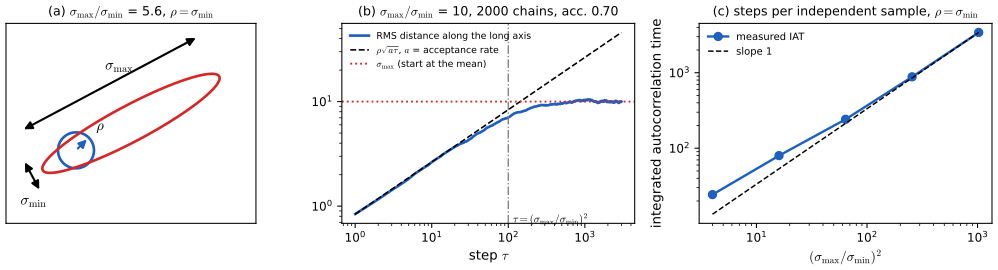
fig11_10. Download: PDF · SVG11.3 Gibbs sampling
pp. 542–546 Gibbs sampling (Geman and Geman, 1984) updates one variable at a time by drawing it from its full conditional \(p(z_i\given\mathbf z_{\setminus i})\), the distribution of \(z_i\) given all the other variables at their current values. For three variables, one sweep draws \(z_1^{(\tau+1)}\) from
\[ p(z_1\given z_2^{(\tau)},z_3^{(\tau)}), \tag{11.46} \] \[ \text{then }z_2^{(\tau+1)}\text{ from }p(z_2\given z_1^{(\tau+1)},z_3^{(\tau)}), \tag{11.47} \] \[ \text{then }z_3^{(\tau+1)}\text{ from }p(z_3\given z_1^{(\tau+1)},z_2^{(\tau+1)}), \tag{11.48} \]always using the newest values.
Algorithm 11.6 (Gibbs sampling) p. 543
- Initialise \(\{z_i:i=1,\dots,M\}\).
- For \(\tau=1,\dots,T\) and \(j=1,\dots,M\) in turn: draw \[ z_j^{(\tau+1)}\sim p\big(z_j\given z_1^{(\tau+1)},\dots,z_{j-1}^{(\tau+1)},z_{j+1}^{(\tau)},\dots,z_M^{(\tau)}\big). \]
Variants: random scan (pick \(j\) at random at each step) and blocked Gibbs (update a group of variables jointly from their joint conditional).
Erratum. Some printings write \(p(z_i\given\{\mathbf z_{\setminus i})\) on p. 544 (a stray brace); it is \(p(z_i\given\mathbf z_{\setminus i})\).
Result 11.20 (Gibbs updates leave \(p\) invariant; they are Metropolis-Hastings steps that are always accepted; Exercise 11.11) p. 544, (11.49)
Let \(B_k\) be the update of variable \(z_k\) from \(p(z_k\given\mathbf z_{\setminus k})\). Then:
(a) \(B_k\) is the Metropolis-Hastings transition with proposal \(q_k(\mathbf z^\star\given\mathbf z)\)
(b) \(B_k\) satisfies detailed balance with respect to \(p\), hence leaves \(p\) invariant;
(c) consequently the systematic scan \(B_1B_2\cdots B_M\) and the random scan \(\frac1M\sum_kB_k\) leave \(p\) invariant; the random scan (and the forward-backward scan) is reversible, the systematic scan in general is not.
Proof
(a) Use \(p(\mathbf z)\)
(b) Directly (the solution of Exercise 11.11): \(B_k(\mathbf z,\mathbf z')\)
which is symmetric under exchanging \(z_k\) and \(z_k'\) (the common \(\mathbf z_{\setminus k}=\mathbf z'_{\setminus k}\) is untouched), so it equals \(p(\mathbf z')B_k(\mathbf z',\mathbf z)\). For pairs that differ outside coordinate \(k\), both sides are 0. Invariance then follows from Result 11.16. The book's own argument is the same fact read differently: the update leaves the marginal of \(\mathbf z_{\setminus k}\) untouched and redraws \(z_k\) from the correct conditional, so if \(\mathbf z\sim p\) before, the pair (marginal, conditional) and hence the joint is \(p\) after.
(c) By Result 11.18: invariance for both; detailed balance for the mixture (random scan) and for the palindromic composition \(B_1\cdots B_MB_M\cdots B_1\); not in general for \(B_1\cdots B_M\). ∎
Ergodicity p. 544. The book's sufficient condition is that no conditional distribution is zero anywhere. For a density on \(\R^M\), a convenient version is: if \(p(\mathbf z)\gt0\) for all \(\mathbf z\), then after one sweep the chain has moved from \(\mathbf z\) to \(\mathbf z'\) with density \(\prod_{j}p(z_j'\given z'_1,\dots,z'_{j-1},z_{j+1},\dots,z_M)\)
Gibbs sampling a correlated Gaussian pp. 544–545, Figure 11.11
The book argues that the step size of Gibbs sampling is set by the conditional widths \(l\), while the distribution extends a distance \(L\) along its long axis, so that a random walk needs about \((L/l)^2\) steps. For a bivariate Gaussian everything can be computed exactly.
Result 11.21 (Gibbs on a bivariate Gaussian) pp. 544–545
Let \((z_1,z_2)\) be Gaussian with means \(\mu_1,\mu_2\), standard deviations \(\sigma_1,\sigma_2\) and correlation \(\rho\). (a) The full conditionals are
\[ z_1\given z_2\sim\N\Big(\mu_1+\rho\frac{\sigma_1}{\sigma_2}(z_2-\mu_2),\;\sigma_1^2(1-\rho^2)\Big),\qquad z_2\given z_1\sim\N\Big(\mu_2+\rho\frac{\sigma_2}{\sigma_1}(z_1-\mu_1),\;\sigma_2^2(1-\rho^2)\Big). \](b) Under the systematic scan, the sequence \(z_1^{(\tau)}\) is a first-order autoregression with coefficient \(\rho^2\): its lag-\(k\) autocorrelation is \(\rho^{2k}\), and its integrated autocorrelation time is
\[ \tau_{\rm int}=\frac{1+\rho^2}{1-\rho^2}. \](c) With unit variances, the conditional width is \(l=\sqrt{1-\rho^2}\) and the standard deviation along the long axis is \(L=\sqrt{1+\rho}\), so \((L/l)^2=1/(1-\rho)\); as \(\rho\to1\), \(\tau_{\rm int}\sim1/(1-\rho)\sim(L/l)^2\), confirming the book's estimate. For \(\rho=0.9\) and \(0.99\): \(\tau_{\rm int}=9.53\) and \(99.5\), against \((L/l)^2=10\) and \(100\). If instead \(L\) is taken to be the marginal standard deviation (1 here), as in the book's wording "marginal distributions of width \(L\)" and in our figures, then \((L/l)^2=1/(1-\rho^2)\) and \(\tau_{\rm int}=(1+\rho^2)(L/l)^2\approx2(L/l)^2\): the same order.
Proof
(a) The conditional of one block of a Gaussian given the other (Section 2.3.1; toolkit) with covariance entries \(\Sigma_{11}=\sigma_1^2\), \(\Sigma_{12}=\rho\sigma_1\sigma_2\), \(\Sigma_{22}=\sigma_2^2\): the mean is \(\mu_1+\Sigma_{12}\Sigma_{22}^{-1}(z_2-\mu_2)\) and the variance \(\Sigma_{11}-\Sigma_{12}^2/\Sigma_{22}\)
(b) Standardise (\(\mu_i=0\), \(\sigma_i=1\)); Gibbs sampling commutes with this affine change of each coordinate. One sweep is \(z_1'=\rho z_2+s\nu_1\), \(z_2'=\rho z_1'+s\nu_2\), with \(s=\sqrt{1-\rho^2}\) and independent standard normals \(\nu_1,\nu_2\). Substituting the previous sweep's \(z_2=\rho z_1+s\nu_2^{\rm old}\): \(z_1'=\rho^2z_1+\rho s\nu^{\rm old}_2+s\nu_1\), an autoregression with coefficient \(\phi=\rho^2\) and noise independent of \(z_1\). In stationarity the lag-\(k\) autocorrelation is \(\phi^k\), and Result 11.2 gives \(\tau_{\rm int}=(1+\phi)/(1-\phi)\).
(c) The conditional variance is \(1-\rho^2\). The covariance matrix \(\begin{pmatrix}1&\rho\\\rho&1\end{pmatrix}\) has eigenvalues \(1\pm\rho\) with eigenvectors along the diagonals, so the long-axis standard deviation is \(\sqrt{1+\rho}\). Then \((L/l)^2=(1+\rho)/(1-\rho^2)=1/(1-\rho)\), and \(\tau_{\rm int}=(1+\rho^2)/\{(1-\rho)(1+\rho)\}\), whose ratio to \(1/(1-\rho)\) is \((1+\rho^2)/(1+\rho)\to1\). ∎
If the variables were uncorrelated, Gibbs sampling would produce independent draws at every sweep. For this toy problem a rotation would decorrelate them, but in real problems such a transformation is not available p. 544.
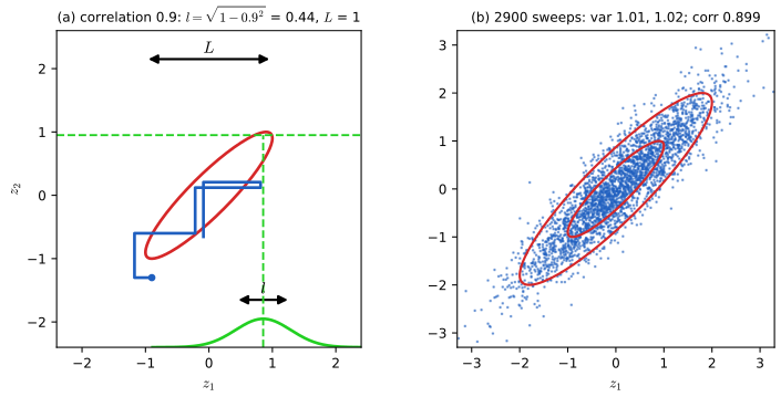
fig11_11. Download: PDF · SVG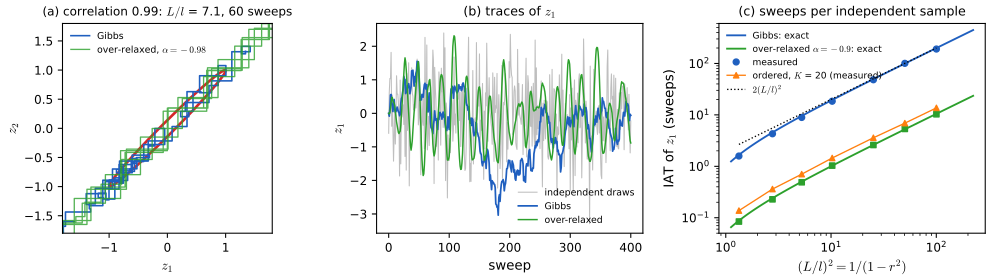
fig11_12. Download: PDF · SVGOver-relaxation p. 545, (11.50)
Adler's (1981) over-relaxation applies when the full conditionals are Gaussian. This is more general than a Gaussian joint: \(p(z,y)\propto\exp(-z^2y^2-z^2-y^2)\) is not Gaussian, but each conditional is (for example \(z\given y\sim\N(0,\{2(1+y^2)\}^{-1})\)). (The book's example \(\exp(-z^2y^2)\) has Gaussian conditionals but cannot be normalised, since \(\int\!\int e^{-z^2y^2}\d z\,\d y\)
with \(\nu\sim\N(0,1)\) and \(-1\lt\alpha\lt1\). For \(\alpha=0\) this is the Gibbs update; for \(\alpha\lt0\) the new value is pushed to the other side of the conditional mean.
Erratum. Some printings write \(\alpha_i^2\) in the last term of (11.50); it is \(\alpha^2\).
Result 11.22 (over-relaxation leaves \(p\) invariant; Exercise 11.14) p. 545
(a) If \(z_i\given\mathbf z_{\setminus i}\)
Proof
(a) Given \(\mathbf z_{\setminus i}\), \(\mu_i\) and \(\sigma_i\) are constants and \(z_i'\) is a linear combination of the independent Gaussians \(z_i\) and \(\nu\), so it is Gaussian, with mean \(\mu_i+\alpha\cdot0+0=\mu_i\) and variance \(\alpha^2\sigma_i^2+\sigma_i^2(1-\alpha^2)\)
(b) Given \(\mathbf z_{\setminus i}\), the pair \((z_i,z_i')\) is bivariate Gaussian with both marginals \(\N(\mu_i,\sigma_i^2)\) and covariance \(\E[(z_i-\mu_i)(z_i'-\mu_i)]=\alpha\sigma_i^2\). A bivariate Gaussian with equal marginals is symmetric under exchanging its two coordinates, so \(p(z_i\given\mathbf z_{\setminus i})T(z_i,z_i')\)
(c) With standardised variables, each over-relaxed update is linear plus Gaussian noise, so a sweep is a linear autoregression \(\mathbf z'=\mathbf A\mathbf z+\bm\eta\). I computed its stationary covariance \(\mathbf S\) (from \(\mathbf S\)
With \(\alpha\) close to \(-1\), each update reflects the variable to the other side of its conditional mean with little noise, so successive sweeps keep moving in the same direction along the long axis instead of diffusing: directed motion replaces the random walk. Ordered over-relaxation (Neal, 1999) achieves a similar effect for non-Gaussian conditionals: draw several values from the conditional, sort them together with the current value, and move to the value in the mirror-image rank.
Gibbs sampling on graphical models, ICM and blocking pp. 545–546
On a graphical model, the full conditional of a node involves only its Markov blanket: its neighbours in an undirected graph, and its parents, children and co-parents in a directed graph (the book's Figure 11.12).
Filling the gap 11.10: full conditionals depend only on the Markov blanket p. 545, Figure 11.12
Derivation
Directed graph. From (11.4), \(p(z_i\given\mathbf z_{\setminus i})\)
which involves \(z_i\), its parents, its children and the children's other parents (co-parents), and nothing else.
Undirected graph. With \(p(\mathbf z)=\frac1Z\prod_C\psi_C(\mathbf z_C)\), the same cancellation leaves \(\prod_{C\ni i}\psi_C(\mathbf z_C)\), a function of \(z_i\) and its neighbours.
Consequences. (i) A Gibbs update costs only the size of the blanket. (ii) For directed models built from log-concave conditionals with log-concave dependence on the parents, each factor above is log-concave in \(z_i\), and a product of log-concave functions is log-concave (sum of concave logarithms), so scalar nodes can be updated by adaptive rejection sampling (Section 11.1.3). (iii) If each child's conditional is conjugate to the node's prior, the product is of the same family as \(p(z_i\given\mathrm{pa}_i)\) and can be sampled directly (Exercise 11.13 is an example). ∎
Iterated conditional modes (ICM, Section 8.3.3) replaces each draw by the mode of the conditional: a greedy, deterministic relative of Gibbs sampling that climbs to a local maximum of \(p\) instead of sampling it. Blocking Gibbs (Jensen, Kong and Kjærulff, 1995) updates groups of variables jointly from their joint conditional; the proof of Result 11.20 goes through unchanged with \(z_k\) replaced by a block \(\mathbf z_B\) (marginal of the rest unchanged, block drawn from the correct conditional). Strongly dependent variables put in the same block no longer slow each other down; in the bivariate Gaussian, one block of both variables gives independent draws.
11.4 Slice sampling
pp. 546–548 Metropolis is sensitive to its step size. Slice sampling (Neal, 2003) adapts the step size automatically. It adds an auxiliary variable \(u\) and samples uniformly from the region under the graph of \(\widetilde p\):
\[ \widehat p(z,u)=\begin{cases}1/Z_p&\text{if }0\le u\le\widetilde p(z),\\ 0&\text{otherwise,}\end{cases} \tag{11.51} \]with \(Z_p=\int\widetilde p(z)\,\d z\). Its marginal is
\[ \int\widehat p(z,u)\,\d u=\int_0^{\widetilde p(z)}\frac1{Z_p}\,\d u=\frac{\widetilde p(z)}{Z_p}=p(z), \tag{11.52} \]so sampling \((z,u)\) and discarding \(u\) samples \(p\) (this is Result 11.6 again). Under \(\widehat p\), the conditional of \(u\) given \(z\) is uniform on \([0,\widetilde p(z)]\), and the conditional of \(z\) given \(u\) is uniform on the slice \(S_u=\{z:\widetilde p(z)\gt u\}\). Gibbs sampling of \((z,u)\) alternates the two (Figure 11.13a). The second draw is the hard part, since the slice may be a union of intervals whose ends are unknown; it is enough to replace it by any update of \(z\) that leaves the uniform distribution on \(S_u\) invariant.
Algorithm 11.7 (slice sampling with stepping out and shrinkage; Neal, 2003) pp. 547–548
- Draw \(u\) uniform on \((0,\widetilde p(z^{(\tau)}))\).
- Stepping out. Place an interval of width \(w\) around \(z^{(\tau)}\) at a random position: \(z_{\min}=z^{(\tau)}-wv\), \(z_{\max}=z_{\min}+w\), with \(v\) uniform on \((0,1)\). While \(\widetilde p(z_{\min})\gt u\), set \(z_{\min}\leftarrow z_{\min}-w\); while \(\widetilde p(z_{\max})\gt u\), set \(z_{\max}\leftarrow z_{\max}+w\).
- Shrinkage. Repeat: draw \(z'\) uniform on \((z_{\min},z_{\max})\). If \(\widetilde p(z')\gt u\), set \(z^{(\tau+1)}=z'\) and stop. Otherwise, if \(z'\lt z^{(\tau)}\) set \(z_{\min}=z'\), else set \(z_{\max}=z'\).
For several variables, apply this to each coordinate in turn, using a function proportional to \(p(z_i\given\mathbf z_{\setminus i})\) (p. 548).
Result 11.23 (stepping out and shrinkage leave the slice distribution invariant) p. 547
Fix \(u\) and let \(S=S_u\). The update \(z\mapsto z'\) of steps 2–3 has a transition density \(T_u(z,z')\) on \(S\) that is symmetric, \(T_u(z,z')=T_u(z',z)\) for \(z,z'\in S\). Hence the uniform distribution on \(S\) satisfies detailed balance, and the whole slice-sampling update (step 1 then steps 2–3) leaves \(\widehat p(z,u)\), and therefore \(p(z)\), invariant.
Proof
Stepping out produces the same interval from \(z\) and from \(z'\). The random initial placement fixes a grid \(G=\{z_{\min}^{0}+jw:j\in\mathbb Z\}\) whose offset modulo \(w\) is uniform, whatever the current point: the initial interval is the grid cell containing the current point. Stepping out then moves the left end down the grid until it hits a grid point outside \(S\), and the right end up the grid likewise. So the final interval is \((L,R]\) where \(L\) is the largest grid point \(\le z\) outside \(S\) and \(R\) the smallest grid point \(\gt z\) outside \(S\), and every grid point strictly between \(L\) and \(R\) lies in \(S\). Now take any \(z'\in S\cap(L,R)\). Starting from \(z'\) with the same grid, the largest grid point \(\le z'\) outside \(S\) is again \(L\) (all grid points in \((L,z']\) are in \(S\)), and similarly for \(R\). Since the grid offset has the same distribution from either starting point, \(\Pr(\text{interval }I\given z)\)
Shrinkage is symmetric. Fix the interval \(I\) and two points \(z,z'\in S\cap I\). A run from \(z\) that ends at \(z'\) consists of rejected points \(y_1,\dots,y_m\notin S\), each drawn uniformly from the current interval, followed by \(z'\). At each rejection the interval keeps the side containing the current point \(z\). Because the run ends by drawing \(z'\), every interval along the way contains \(z'\) too, so no \(y_j\) lies between \(z\) and \(z'\); hence "\(y_j\lt z\)" and "\(y_j\lt z'\)" agree, and starting from \(z'\) the same rejected points shrink the interval in exactly the same way, ending with an interval from which \(z\) can be drawn. The density of the run is the product of \(1/(\text{length of the current interval})\) over its draws, and these lengths are the same for the run from \(z\) and its mirror run from \(z'\). Summing (integrating) over all sequences of rejected points gives \(\Pr(z\to z'\given I)=\Pr(z'\to z\given I)\) as densities.
Conclusion. \(T_u(z,z')\)
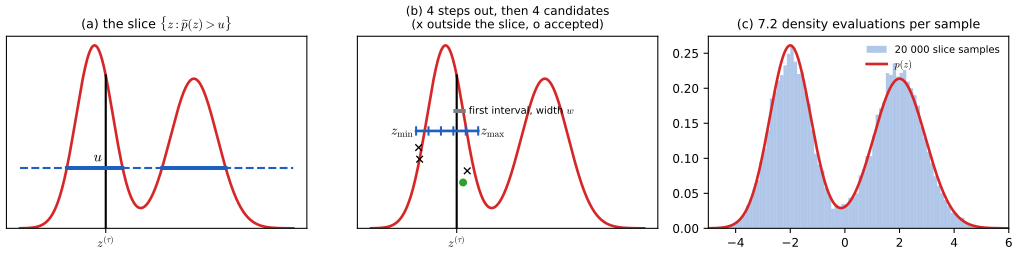
fig11_13. Download: PDF · SVGThe width \(w\) affects only efficiency: if it is too small, stepping out takes more steps (linear in the slice width divided by \(w\)); if too large, shrinkage takes more rejections (logarithmic in \(w\) divided by the slice width). Neal (2003) also describes a doubling procedure and limits on the number of steps, which need an extra acceptance check.
11.5 The hybrid Monte Carlo algorithm
p. 548 Random-walk proposals travel a distance proportional to the square root of the number of steps, and larger steps are rejected more often. Hybrid Monte Carlo (also called Hamiltonian Monte Carlo, HMC) makes long, directed moves that are still accepted with high probability, by simulating a physical system whose potential energy is \(-\ln p\). It needs the gradient of \(\ln\widetilde p\), and applies to continuous variables.
11.5.1 Dynamical systems
pp. 548–551 Regard \(\mathbf z\) as the position of a particle moving in continuous time \(\tau\), and introduce a momentum (here simply the velocity, unit mass) for each coordinate:
\[ r_i=\frac{\d z_i}{\d\tau}. \tag{11.53} \]The pair \((\mathbf z,\mathbf r)\) lives in phase space. Write the target as
\[ p(\mathbf z)=\frac1{Z_p}\exp\big(-E(\mathbf z)\big), \tag{11.54} \]which defines the potential energy \(E(\mathbf z)=-\ln\widetilde p(\mathbf z)\) (any positive density can be written this way). The force is minus the gradient of the potential, and Newton's law says it equals the rate of change of momentum:
\[ \frac{\d r_i}{\d\tau}=-\frac{\partial E(\mathbf z)}{\partial z_i}. \tag{11.55} \]With the kinetic energy and the Hamiltonian (total energy)
\[ K(\mathbf r)=\frac12\lVert\mathbf r\rVert^2=\frac12\sum_ir_i^2, \tag{11.56} \] \[ H(\mathbf z,\mathbf r)=E(\mathbf z)+K(\mathbf r), \tag{11.57} \]the dynamics take Hamilton's form
\[ \frac{\d z_i}{\d\tau}=\frac{\partial H}{\partial r_i}, \tag{11.58} \] \[ \frac{\d r_i}{\d\tau}=-\frac{\partial H}{\partial z_i}. \tag{11.59} \](Exercise 11.15: \(\partial H/\partial r_i\)
The second key property, Liouville's theorem, concerns the flow field in phase space,
\[ \mathbf V=\Big(\frac{\d\mathbf z}{\d\tau},\frac{\d\mathbf r}{\d\tau}\Big), \tag{11.61} \]whose divergence vanishes:
\[ \operatorname{div}\mathbf V=\sum_i\Big\{\frac{\partial}{\partial z_i}\frac{\d z_i}{\d\tau}+\frac{\partial}{\partial r_i}\frac{\d r_i}{\d\tau}\Big\}=\sum_i\Big\{\frac{\partial}{\partial z_i}\frac{\partial H}{\partial r_i}-\frac{\partial}{\partial r_i}\frac{\partial H}{\partial z_i}\Big\}=0 . \tag{11.62} \]Erratum. In some printings the \(+\) and \(-\) in the second line of (11.62) are swapped; the form above (mixed second derivatives of \(H\) cancelling) is correct.
The joint distribution on phase space that HMC targets is
\[ p(\mathbf z,\mathbf r)=\frac1{Z_H}\exp\big(-H(\mathbf z,\mathbf r)\big). \tag{11.63} \]Result 11.24 (Hamiltonian flow preserves energy, volume and the distribution (11.63); Exercise 11.16) pp. 549–551, (11.60)–(11.63)
Let \(\Phi_t\) map a point of phase space to its position after following (11.58)–(11.59) for time \(t\), with \(E\) twice continuously differentiable. Then (a) \(H\circ\Phi_t=H\); (b) \(\Phi_t\) preserves volume: \(\det\big(\partial\Phi_t/\partial(\mathbf z,\mathbf r)\big)\)
Proof
(a) is (11.60).
(b) Write \(\mathbf x=(\mathbf z,\mathbf r)\), \(\dot{\mathbf x}=\mathbf V(\mathbf x)\), and let \(\mathbf J(t)\)
using the cyclic property of the trace (toolkit) and (11.62). So \(\det\mathbf J(t)=\det\mathbf J(0)=1\) for all \(t\): the image of any region has the same volume as the region.
(c) \(\Phi_t\) is a bijection with inverse \(\Phi_{-t}\) (run the flow backwards). By the change-of-variables formula (11.9) with unit Jacobian, the density of \(\mathbf y=\Phi_t(\mathbf x)\) is \(p(\Phi_{-t}(\mathbf y))\), and by (a) \(H(\Phi_{-t}(\mathbf y))=H(\mathbf y)\), so the density is \(e^{-H(\mathbf y)}/Z_H\), the same as before. This is the book's argument (a small region keeps its volume and its value of \(H\)) made exact.
(d) \(e^{-H}\)
Because \(H\) is constant along trajectories, the dynamics alone are not ergodic: they stay on one energy level. Redrawing \(\mathbf r\) from \(p(\mathbf r\given\mathbf z)\)
The leapfrog integrator p. 551. The equations must be solved numerically. With step size \(\epsilon\), one leapfrog step is
\[ \widehat r_i(\tau+\epsilon/2)=\widehat r_i(\tau)-\frac{\epsilon}{2}\frac{\partial E}{\partial z_i}\big(\widehat{\mathbf z}(\tau)\big), \tag{11.64} \] \[ \widehat z_i(\tau+\epsilon)=\widehat z_i(\tau)+\epsilon\,\widehat r_i(\tau+\epsilon/2), \tag{11.65} \] \[ \widehat r_i(\tau+\epsilon)=\widehat r_i(\tau+\epsilon/2)-\frac{\epsilon}{2}\frac{\partial E}{\partial z_i}\big(\widehat{\mathbf z}(\tau+\epsilon)\big). \tag{11.66} \]In a sequence of steps the closing half-step of one and the opening half-step of the next merge into one full momentum step, so positions and momenta "leapfrog" over each other, and only one new gradient is needed per step. Integrating for time \(\tau\) takes \(\tau/\epsilon\) steps.
Result 11.25 (properties of the leapfrog integrator) pp. 551–552, (11.64)–(11.66)
Let \(\Psi_\epsilon\) denote one leapfrog step (11.64)–(11.66), and \(\Psi_\epsilon^L\) a sequence of \(L\) steps. Then:
(a) volume preservation: \(\det\big(\partial\Psi_\epsilon/\partial(\mathbf z,\mathbf r)\big)\)
(b) time reversibility: \(\Psi_{-\epsilon}\circ\Psi_\epsilon=\mathrm{id}\), hence \(\Psi_{-\epsilon}^L=(\Psi_\epsilon^L)^{-1}\);
(c) accuracy: one step agrees with the exact flow \(\Phi_\epsilon\) up to \(O(\epsilon^3)\); over a fixed time \(\tau=L\epsilon\) the error in \((\mathbf z,\mathbf r)\), and in \(H\), is \(O(\epsilon^2)\);
(d) the Gaussian case: for \(E(z)=z^2/(2\sigma^2)\) in one dimension, the leapfrog iteration is stable iff \(\epsilon\lt2\sigma\), and then it conserves exactly the modified energy \(\widetilde H\)
Proof
(a) Each of (11.64), (11.65), (11.66) changes one block of variables by an amount that depends only on the other block: \((\mathbf z,\mathbf r)\mapsto(\mathbf z,\mathbf r+\mathbf g(\mathbf z))\) or \((\mathbf z,\mathbf r)\mapsto(\mathbf z+\mathbf h(\mathbf r),\mathbf r)\). Such a map is a shear (Figure 11.14 of the book): its Jacobian matrix is block triangular, \(\begin{pmatrix}\mathbf I&\mathbf 0\\\partial\mathbf g/\partial\mathbf z&\mathbf I\end{pmatrix}\) or \(\begin{pmatrix}\mathbf I&\partial\mathbf h/\partial\mathbf r\\\mathbf 0&\mathbf I\end{pmatrix}\), with determinant 1. A composition of maps with unit Jacobian determinant has unit Jacobian determinant (the determinant of a product is the product of the determinants).
(b) Let \((\mathbf z',\mathbf r')\)
(c) Let \(\mathbf g=\nabla E(\mathbf z)\) and \(\mathbf A=\nabla^2E(\mathbf z)\). The exact flow, by Taylor expansion of (11.53), (11.55): \(\mathbf z(\epsilon)\)
(d) Let \(\omega=1/\sigma\). One step is linear, \((z',r')^\T=\mathbf M(z,r)^\T\) with
\[ \mathbf M=\begin{pmatrix}1-\frac{\epsilon^2\omega^2}{2}&\epsilon\\ -\epsilon\omega^2\big(1-\frac{\epsilon^2\omega^2}{4}\big)&1-\frac{\epsilon^2\omega^2}{2}\end{pmatrix}, \]obtained by composing the three shears. \(\det\mathbf M=1\) (part a) and \(\Tr\mathbf M=2-\epsilon^2\omega^2\). The eigenvalues \(\lambda\) solve \(\lambda^2-(\Tr\mathbf M)\lambda+1=0\). If \(|\Tr\mathbf M|\lt2\), i.e. \(0\lt\epsilon\omega\lt2\), they are complex conjugates of modulus 1 and the iteration is a (sheared) rotation: bounded. If \(\epsilon\omega\gt2\), \(\Tr\mathbf M\lt-2\) and there is a real eigenvalue of modulus \(\gt1\): exponential growth. (In my run, 200 steps with \(\epsilon=1.9\sigma\) stayed bounded, with \(\epsilon=2.1\sigma\) reached \(|z|\approx10^{54}\).) For the conserved quantity, check that \(\mathbf M^\T\mathbf Q\mathbf M=\mathbf Q\) for \(\mathbf Q\)
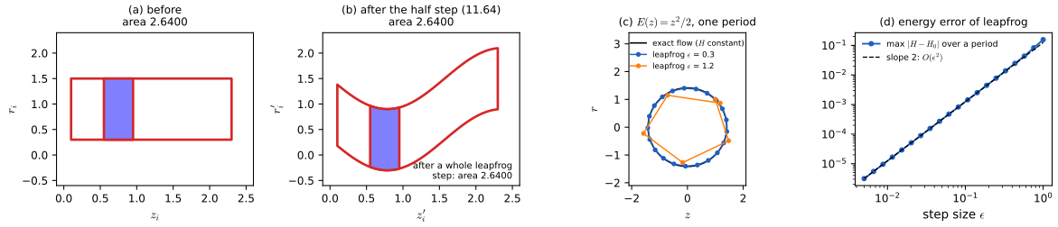
fig11_14. Download: PDF · SVGWhy gradients help p. 551. The cost of a gradient is usually a small constant multiple of the cost of evaluating \(E\) (reverse-mode differentiation), whatever the dimension \(D\), while it carries \(D\) numbers of information instead of one. Hamiltonian dynamics uses this information to move along the distribution rather than probing at random.
11.5.2 Hybrid Monte Carlo
pp. 552–554 Hybrid Monte Carlo (Duane et al., 1987; Neal, 1996) corrects the leapfrog error with a Metropolis test. From \((\mathbf z,\mathbf r)\), run \(L\) leapfrog steps to a candidate \((\mathbf z^\star,\mathbf r^\star)\) and accept it with probability
\[ \min\big(1,\exp\{H(\mathbf z,\mathbf r)-H(\mathbf z^\star,\mathbf r^\star)\}\big). \tag{11.67} \]If the integration were exact, \(H\) would not change and every candidate would be accepted. For detailed balance, the integration direction is chosen at random: forwards (\(+\epsilon\)) or backwards (\(-\epsilon\)) with probability \(\frac12\) each.
Algorithm 11.8 (hybrid Monte Carlo) pp. 551–553
- Draw a fresh momentum \(\mathbf r\sim\N(\mathbf 0,\mathbf I)\) (the Gibbs step).
- Choose \(\pm\epsilon\) with probability \(\frac12\) each (and, to avoid periodic orbits, draw the magnitude of \(\epsilon\) from a small interval).
- Apply \(L\) leapfrog steps (11.64)–(11.66) to get \((\mathbf z^\star,\mathbf r^\star)\).
- Accept \(\mathbf z^\star\) with probability (11.67); otherwise keep \(\mathbf z\). Discard the momentum.
Result 11.26 (hybrid Monte Carlo satisfies detailed balance; Exercise 11.17) pp. 552–553, (11.68)–(11.69)
Let \(\mathcal R\) be a small region of phase space of volume \(\delta V\) that \(L\) leapfrog steps of size \(\epsilon\) map to \(\mathcal R'\). Starting from (11.63), the probability of moving from \(\mathcal R\) to \(\mathcal R'\) in one HMC transition (steps 2–4) is
\[ \frac{1}{Z_H}\exp\big(-H(\mathcal R)\big)\,\delta V\,\frac12\min\big\{1,\exp\big(H(\mathcal R)-H(\mathcal R')\big)\big\}, \tag{11.68} \]and the probability of moving from \(\mathcal R'\) back to \(\mathcal R\) (integrating backwards) is
\[ \frac{1}{Z_H}\exp\big(-H(\mathcal R')\big)\,\delta V\,\frac12\min\big\{1,\exp\big(H(\mathcal R')-H(\mathcal R)\big)\big\}. \tag{11.69} \]The two are equal. More precisely, for every bounded function \(g\), \(\E[g(\mathbf x,\mathbf x')]\)
Proof
The book's version. Both (11.68) and (11.69) equal \(\frac{\delta V}{2Z_H}\min\{e^{-H(\mathcal R)},e^{-H(\mathcal R')}\}\), because \(e^{-a}\min(1,e^{a-b})=\min(e^{-a},e^{-b})\). The volume factor \(\delta V\) is the same in both because the leapfrog map preserves volume (Result 11.25a), and the backward integration from \(\mathcal R'\) lands exactly on \(\mathcal R\) because it inverts the forward one (Result 11.25b). The factor \(\frac12\) is the probability of choosing the right direction. (Svensen and Bishop's official solution splits the cases \(H(\mathcal R)\gt H(\mathcal R')\) and \(\lt\); the identity above does both at once.)
An exact version, which also handles overlapping regions (the book's last remark). Let \(\Psi=\Psi^L_\epsilon\), so \(\Psi^{-1}=\Psi^L_{-\epsilon}\), let \(\pi=e^{-H}/Z_H\), and \(a(\mathbf x,\mathbf y)\)
In the second integral substitute \(\mathbf x=\Psi\mathbf y\), with \(\d\mathbf x=\d\mathbf y\) (unit Jacobian): it becomes \(\tfrac12\int\pi(\Psi\mathbf y)a(\Psi\mathbf y,\mathbf y)g(\Psi\mathbf y,\mathbf y)\,\d\mathbf y\). Since \(\pi(\mathbf u)a(\mathbf u,\mathbf v)\)
Why both directions are needed. With \(+\epsilon\) only, the move \(\mathbf x\to\Psi\mathbf x\) would have no reverse move \(\Psi\mathbf x\to\mathbf x\) (that needs \(\Psi^{-1}\)), and detailed balance would fail. Equivalently one may always integrate forwards and then negate the momentum, which makes the proposal an involution; the negation is harmless because the next step 1 redraws \(\mathbf r\) and \(K(-\mathbf r)=K(\mathbf r)\). ∎
Erratum. In the first printing the arguments of the exponentials inside the minima of (11.68) and (11.69) have the wrong sign; the corrected forms are given above (this is noted in Svensen and Bishop's solution to Exercise 11.17).
Ergodicity p. 553. For some step sizes the leapfrog map returns exactly to its start after \(L\) steps (in the Gaussian case of Result 11.25d this happens when \(L\) times the rotation angle per step is a multiple of \(2\pi\)), and then \(\mathbf z\) never moves however the momentum is refreshed. Drawing \(\epsilon\) at random from a small interval at each iteration rules this out.
Filling the gap 11.11: HMC needs about \(\sigma_{\max}/\sigma_{\min}\) leapfrog steps, random-walk Metropolis about \((\sigma_{\max}/\sigma_{\min})^2\) pp. 553–554, (11.70)
The book's comparison uses an independent Gaussian with Hamiltonian
\[ H(\mathbf z,\mathbf r)=\frac12\sum_i\frac{z_i^2}{\sigma_i^2}+\frac12\sum_ir_i^2 . \tag{11.70} \]Derivation
Rotational invariance. If \(\mathbf z=\mathbf U\mathbf y\) with \(\mathbf U\) orthogonal and we also rotate \(\mathbf r=\mathbf U\mathbf s\), then \(K\) is unchanged and the leapfrog equations in \((\mathbf y,\mathbf s)\) have the same form; so a correlated Gaussian behaves like (11.70) in its principal axes. During integration the pairs \((z_i,r_i)\) evolve independently, each a harmonic oscillator with \(\omega_i=1/\sigma_i\), but acceptance depends on the total \(H\), so one badly integrated coordinate is enough to cause rejection.
Step size. By Result 11.25d, coordinate \(i\) is stable only if \(\epsilon\lt2\sigma_i\), and its energy error is of order \((\epsilon/\sigma_i)^2\). So \(\epsilon\) must be a fraction of \(\sigma_{\min}\).
Trajectory length. Coordinate \(i\) oscillates with period \(2\pi\sigma_i\). To reach a nearly independent value along the widest direction, the trajectory must run for about a quarter period there, time of order \(\sigma_{\max}\), which takes \(L\)
Comparison. Random-walk Metropolis with scale \(s\approx\sigma_{\min}\) needs about \((\sigma_{\max}/\sigma_{\min})^2\) steps (Filling the gap 11.9). With \(\sigma_{\max}/\sigma_{\min}=100\), that is roughly \(10^4\) steps against \(10^2\) leapfrog steps. In \(D\) dimensions the accumulated energy error requires \(\epsilon\) to shrink like \(D^{-1/4}\) to keep the acceptance rate fixed (Neal, 2011), against \(D^{-1/2}\) for random-walk Metropolis, so the advantage grows with dimension. ∎
11.6 Estimating the partition function
pp. 554–555 Samplers need \(p\) only up to its normalising constant. For model comparison, however, the constant is the quantity of interest. Write
\[ p_E(\mathbf z)=\frac1{Z_E}\exp\big(-E(\mathbf z)\big), \tag{11.71} \]where \(Z_E\) is the partition function. If \(\mathbf z\) are the parameters \(\bm\theta\) of a model and \(\exp(-E(\bm\theta))\)
Importance sampling from a distribution \(p_G\) with energy \(G\) gives
\[ \frac{Z_E}{Z_G}=\frac{\sum_{\mathbf z}\exp(-E(\mathbf z))}{\sum_{\mathbf z}\exp(-G(\mathbf z))}=\frac{\sum_{\mathbf z}\exp(-E(\mathbf z)+G(\mathbf z))\exp(-G(\mathbf z))}{\sum_{\mathbf z}\exp(-G(\mathbf z))}=\E_{G}\big[\exp(-E+G)\big]\simeq\frac1L\sum_l\exp\big(-E(\mathbf z^{(l)})+G(\mathbf z^{(l)})\big), \tag{11.72} \]with \(\mathbf z^{(l)}\) drawn from \(p_G\). If \(Z_G\) is known (a Gaussian, say), this gives \(Z_E\) itself.
Erratum. Some printings omit the factor \(1/L\) on the last line of (11.72), and on the right of (11.73).
Filling the gap 11.12: derivation and accuracy of (11.72) p. 554, (11.72)
Derivation
Derivation. Multiply and divide the summand of \(Z_E=\sum\exp(-E)\) by \(\exp(-G)\), which is allowed wherever \(\exp(-G)\gt0\) (we need \(p_G\gt0\) wherever \(p_E\gt0\)); then divide by \(Z_G\): \(Z_E/Z_G=\sum_{\mathbf z}e^{-E+G}\,p_G(\mathbf z)\), the expectation under \(p_G\) of \(e^{-E+G}\). The last step is the Monte Carlo average (11.2). It is the ratio estimate (11.21) of importance sampling with \(\widetilde p=e^{-E}\) and \(\widetilde q=e^{-G}\).
Accuracy. The weight \(e^{-E+G}=\frac{Z_E}{Z_G}\cdot\frac{p_E}{p_G}\), so by Result 11.1 the relative variance of the estimate is
\[ \frac{\var[\widehat{Z_E/Z_G}]}{(Z_E/Z_G)^2}=\frac1L\Big\{\E_G\Big[\Big(\frac{p_E}{p_G}\Big)^2\Big]-1\Big\}, \]the quantity of Filling the gap 11.6. It is small only if \(p_E/p_G\) varies little, as the book says. For two isotropic Gaussians in \(D=100\) dimensions with standard deviations 2 (\(p_G\)) and 1 (\(p_E\)), the bracket is \((4/\sqrt7)^{100}-1\approx9\times10^{17}\): hopeless.
A useful identity, and a trap. Because \(\E_G[\widehat{Z_E/Z_G}]=Z_E/Z_G\), the estimate is unbiased, but its logarithm is biased downwards: \(\E[\ln\widehat Z]\le\ln\E[\widehat Z]=\ln Z\) by Jensen's inequality (toolkit), so log evidences estimated this way are too small on average. Taking \(p_G\) to be the prior gives the "average likelihood over prior draws" estimate of \(p(\mathcal D)\), usually poor because the posterior is much narrower than the prior. The reverse choice (sampling the posterior and averaging \(1/p(\mathcal D\given\bm\theta)\), the harmonic mean estimator of Newton and Raftery, 1994) is consistent but typically has infinite variance, for the reason in Filling the gap 11.6. ∎
A Markov chain as importance distribution p. 555. Analytically tractable \(p_G\) close to \(p_E\) rarely exist. If a Markov chain with transition density \(T(\mathbf z,\mathbf z')\) and invariant distribution \(p_E\) has produced \(\mathbf z^{(1)},\dots,\mathbf z^{(L)}\), one may use
\[ \frac1{Z_G}\exp\big(-G(\mathbf z)\big)=\frac1L\sum_{l=1}^{L}T(\mathbf z^{(l)},\mathbf z) \tag{11.73} \]in (11.72). This is a mixture of the one-step transition densities from the sampled states. It is normalised (each \(T(\mathbf z^{(l)},\cdot)\) integrates to 1, so \(Z_G=1\) if we take \(\exp(-G)\) equal to the right side), it can be sampled (pick \(l\) at random, then make one transition from \(\mathbf z^{(l)}\)), and, if the \(\mathbf z^{(l)}\) are in equilibrium, its expectation over them is \(\int p_E(\mathbf z')T(\mathbf z',\mathbf z)\,\d\mathbf z'\)
Chaining p. 555. Ratios can only be estimated between distributions that are close. To reach a complex \(p_M\) from a simple \(p_1\) with known \(Z_1\), insert intermediate distributions \(p_2,\dots,p_{M-1}\) (Neal, 1993; Barber and Bishop, 1997) and write
\[ \frac{Z_M}{Z_1}=\frac{Z_2}{Z_1}\,\frac{Z_3}{Z_2}\cdots\frac{Z_M}{Z_{M-1}}, \tag{11.74} \]estimating each factor by (11.72) with neighbouring distributions. A convenient path interpolates the energies,
\[ E_\alpha(\mathbf z)=(1-\alpha)E_1(\mathbf z)+\alpha E_M(\mathbf z),\qquad0\le\alpha\le1, \tag{11.75} \]at a grid of values of \(\alpha\). A single Markov chain can be run through the sequence, moving to the next distribution after some steps, provided it stays close to equilibrium at each stage.
Filling the gap 11.13: why chaining works, and the continuous limit p. 555, (11.74)–(11.75)
Derivation
Variance. If the \(M-1\) ratios are estimated independently with relative variances \(v_k\), the relative variance of their product is \(\prod_k(1+v_k)-1\approx\sum_kv_k\) when all \(v_k\) are small (for independent unbiased factors \(X_k\), \(\E[\prod X_k^2]=\prod\E[X_k^2]\)). Each \(v_k\) is small when neighbouring distributions are close, even though the end points are far apart. Example (my computation): isotropic Gaussians in \(D=100\) with precisions going from \(\frac14\) to 1 along (11.75), sampling each stage from the broader neighbour. The direct estimate has relative variance about \(9\times10^{17}/L\); with \(M=11\), 101 and 1001 distributions equally spaced in \(\alpha\), the summed relative variance is \(27/L\), \(1.1/L\) and \(0.11/L\). For \(M\ge101\), \(M\) times the effort buys a factor of about \(10^{18}\).
Thermodynamic integration. In the limit of a fine grid, differentiate \(\ln Z_\alpha\)
a one-dimensional integral of expectations, each estimated by MCMC at its own \(\alpha\) (Gelman and Meng, 1998). Annealed importance sampling (Neal, 2001) turns the single sweeping chain of the book into an exact importance sampler: the product of the incremental ratios along one sweep is an unbiased estimate of \(Z_M/Z_1\) even when the chain is not in equilibrium. ∎
Exercises
All 17 exercises of Chapter 11 (Bishop, 2006, pp. 556–558), restated in my own words, with complete solutions (hidden). Stars give the book's difficulty and "www" marks the exercises with official solutions. Several solutions are compact versions of the results above, which are linked for more detail.
Exercise 11.1 (★, www). Show that the estimator \(\widehat f\) of (11.2) has mean \(\E[f]\) and variance (11.3).
Solution
Each \(f_l=f(\mathbf z^{(l)})\) has mean \(\E[f]\), so by linearity \(\E[\widehat f]=\frac1L\sum_l\E[f]=\E[f]\). With \(g_l=f_l-\E[f]\), \(\var[\widehat f]=\frac1{L^2}\sum_{l,m}\E[g_lg_m]\); by independence the terms with \(l\ne m\) are \(\E[g_l]\E[g_m]=0\), and the \(L\) diagonal terms are each \(\E[(f-\E f)^2]\). Hence \(\var[\widehat f]=\frac1L\E[(f-\E f)^2]\). Details, and what happens with correlated draws: Result 11.1, Result 11.2.
Exercise 11.2 (★). If \(z\) is uniform on \((0,1)\) and \(y=h^{-1}(z)\) with \(h\) given by (11.6), show that \(y\) has density \(p(y)\).
Solution
\(h\) is nondecreasing; where \(p\gt0\) it is strictly increasing, so \(\Pr(y\le a)\)
\({}=\Pr(h^{-1}(z)\le a)\) \({}=\Pr(z\le h(a))\) \({}=h(a)\), the distribution function of \(p\); differentiating gives \(p(a)\). Equivalently, by (11.5), \(p_y(y)=p_z(h(y))\,|h'(y)|=1\cdot p(y)\). For flat pieces or jumps of \(h\), use the generalised inverse: Result 11.3. Exercise 11.3 (★). Find a transformation \(y=f(z)\) of a uniform \(z\) on \((0,1)\) such that \(y\) has the Cauchy distribution (11.8).
Solution
\(h(y)\)
\({}=\int_{-\infty}^y\frac{\d t}{\pi(1+t^2)}\) \({}=\frac12+\frac1\pi\arctan y\), so \(f(z)=h^{-1}(z)=\tan\{\pi(z-\frac12)\}\). Check: \(z=\frac12+\frac1\pi\arctan y\) gives \(\d z/\d y=\frac{1}{\pi(1+y^2)}\), which is (11.8) by (11.5). See Filling the gap 11.2. ▶ See it in a demo: uniform numbers to Cauchy draws
Exercise 11.4 (★★). For \((z_1,z_2)\) uniform on the unit disc and \((y_1,y_2)\) given by (11.10)–(11.11), show that \((y_1,y_2)\) has the density (11.12).
Solution
With \(s=r^2\) and \(y_i=z_ig(s)\), \(g(s)=\sqrt{-2\ln s/s}\), the Jacobian matrix is \(g\mathbf I+2g'\mathbf z\mathbf z^\T\), with determinant \(g(g+2sg')=-2/s\). So \(p(y_1,y_2)=\frac1\pi\cdot\frac s2\), and since \(y_1^2+y_2^2=sg^2=-2\ln s\), \(s=e^{-(y_1^2+y_2^2)/2}\) and \(p(y_1,y_2)=\frac1{2\pi}e^{-(y_1^2+y_2^2)/2}\), the product of two standard normal densities. The map is a bijection from the punctured disc onto the punctured plane. Full details: Result 11.4.
▶ See it in a demo: Box-Muller
Exercise 11.5 (★, www). Let \(\mathbf z\sim\N(\mathbf 0,\mathbf I_D)\) and \(\bm\Sigma=\mathbf L\mathbf L^\T\) (Cholesky). Show that \(\mathbf y=\bm\mu+\mathbf L\mathbf z\) is \(\N(\bm\mu,\bm\Sigma)\).
Solution
\(\E[\mathbf y]=\bm\mu\) and \(\cov[\mathbf y]\)
\({}=\mathbf L\E[\mathbf z\mathbf z^\T]\mathbf L^\T\) \({}=\mathbf L\mathbf L^\T\) \({}=\bm\Sigma\). A nonsingular affine map of a Gaussian vector is Gaussian: by (11.9) with Jacobian \(|\det\mathbf L|^{-1}=|\bm\Sigma|^{-1/2}\), \(p(\mathbf y)\) \({}=\N(\mathbf L^{-1}(\mathbf y-\bm\mu)\given\mathbf 0,\mathbf I)\,|\bm\Sigma|^{-1/2}\) \({}=\N(\mathbf y\given\bm\mu,\bm\Sigma)\), since \(\mathbf L^{-\T}\mathbf L^{-1}=\bm\Sigma^{-1}\). See Result 11.5. Exercise 11.6 (★★, www). Show that rejection sampling accepts a proposal \(z\) with probability \(\widetilde p(z)/kq(z)\), and that the accepted values have density \(p(z)\).
Solution
Given \(z\), \(u\) is uniform on \([0,kq(z)]\), so \(\Pr(u\le\widetilde p(z)\given z)\)
\({}=\widetilde p(z)/kq(z)\). The joint density of "propose \(z\), accept" is \(q(z)\widetilde p(z)/kq(z)=\widetilde p(z)/k\); integrating, \(\Pr(\text{accept})=Z_p/k\); dividing, \(p(z\given\text{accept})=\widetilde p(z)/Z_p=p(z)\). (Any valid \(k\) works, not only the smallest.) See Result 11.7. ▶ See it in a demo: rejection sampling of a gamma density
Exercise 11.7 (★). Show that if \(y\) is uniform, then \(z=b\tan y+c\) has the Cauchy form (11.16).
Erratum. The printed exercise swaps the roles of \(y\) and \(z\) relative to Section 11.1.2. Also, for the full Cauchy distribution \(y\) must be uniform on \((-\pi/2,\pi/2)\) (or \(y=\pi(u-\frac12)\) with \(u\) uniform on \((0,1)\)); uniform on \([0,1]\) would produce only the values \(c\le z\le c+b\tan1\).
Solution
The map \(y\mapsto z=b\tan y+c\) is increasing from \((-\pi/2,\pi/2)\) onto \(\R\), with inverse \(y=\arctan\{(z-c)/b\}\) and \(\d y/\d z=\frac{1/b}{1+(z-c)^2/b^2}\). With \(p(y)=1/\pi\), (11.5) gives
\[ p(z)=\frac{1}{\pi b}\,\frac{1}{1+(z-c)^2/b^2}, \]which is (11.16) with \(k=1/(\pi b)\), the normalised Cauchy density with location \(c\) and scale \(b\). In rejection sampling the constant \(k\) of (11.16) is then rescaled so that \(kq\ge\widetilde p\) (Filling the gap 11.4).
Exercise 11.8 (★★). Find the coefficients \(k_i\) of the envelope (11.17) from continuity and normalisation.
Solution
On piece \(i\) the unnormalised envelope is \(e^{t_i(z)}\)
\[ C=\sum_i\frac{\widetilde p(z_i)}{\lambda_i}\Big[e^{-\lambda_i(\widehat z_{i-1,i}-z_i)}-e^{-\lambda_i(\widehat z_{i,i+1}-z_i)}\Big],\qquad k_i=\frac{\widetilde p(z_i)}{\lambda_iC}, \]\({}=\widetilde p(z_i)e^{-\lambda_i(z-z_i)}\), with \(\lambda_i=-\ell'(z_i)\), \(\ell=\ln\widetilde p\). Continuity at \(\widehat z_{i,i+1}\): \(k_i\lambda_ie^{-\lambda_i(\widehat z_{i,i+1}-z_i)}\) \({}=k_{i+1}\lambda_{i+1}e^{-\lambda_{i+1}(\widehat z_{i,i+1}-z_{i+1})}\). Since \(\widehat z_{i,i+1}\) is where the tangents meet, \(\ell(z_i)-\lambda_i(\widehat z-z_i)\) \({}=\ell(z_{i+1})-\lambda_{i+1}(\widehat z-z_{i+1})\), which says exactly that \(k_i\lambda_i/\widetilde p(z_i)\) is the same for all \(i\): \(k_i\lambda_i=\widetilde p(z_i)/C\) for one constant \(C\). Normalisation fixes \(C\): with \(\widehat z_{0,1}=-\infty\), \(\widehat z_{n,n+1}=\infty\) (finite because \(\lambda_1\lt0\lt\lambda_n\)). See Result 11.8.
Exercise 11.9 (★★). Devise an algorithm for sampling the piecewise exponential distribution (11.17).
Solution
(11.17) is a mixture of truncated exponentials. Compute the mass \(M_i\) of each piece (the terms of \(C\) above divided by \(C\)). Draw a piece \(i\) with probability \(M_i\) (inverse distribution function of a discrete distribution). Within the piece \([a,b]\), the distribution function is \(F(z)\)
\({}=\{1-e^{-\lambda_i(z-a)}\}/\{1\) \({}-e^{-\lambda_i(b-a)}\}\), so with \(v\) uniform, \(z\) \({}=a-\lambda_i^{-1}\ln[1-v(1-e^{-\lambda_i(b-a)})]\); for the unbounded end pieces, \(z=a-\lambda_n^{-1}\ln v\) (right) and \(z=b+|\lambda_1|^{-1}\ln v\) (left). See Algorithm 11.2 and Filling the gap 11.5. ▶ See it in a demo: adaptive rejection sampling
Exercise 11.10 (★). For the random walk (11.34)–(11.36), show that \(\E[(z^{(\tau)})^2]=\E[(z^{(\tau-1)})^2]+\frac12\) and hence \(\E[(z^{(\tau)})^2]=\tau/2\).
Solution
\(z^{(\tau)}=z^{(\tau-1)}+\xi_\tau\) with \(\xi_\tau\) independent of the past, \(\E\xi_\tau=0\), \(\E\xi_\tau^2=\frac12\). Expanding the square, the cross term has expectation \(2\E[z^{(\tau-1)}]\E[\xi_\tau]=0\), which gives the recursion; with \(z^{(0)}=0\), induction gives \(\tau/2\). See Result 11.15.
▶ See it in a demo: distance travelled against \(\sqrt{\text{steps}}\)
Exercise 11.11 (★★, www). Show that Gibbs sampling satisfies detailed balance (11.40).
Solution
For the update of \(z_k\), \(T(\mathbf z,\mathbf z')\)
\({}=p(z_k'\given\mathbf z_{\setminus k})\) when \(\mathbf z'_{\setminus k}=\mathbf z_{\setminus k}\), and 0 otherwise. Then \(p(\mathbf z)T(\mathbf z,\mathbf z')\) \({}=p(\mathbf z_{\setminus k})\,p(z_k\given\mathbf z_{\setminus k})\) \({}\times p(z_k'\given\mathbf z_{\setminus k})\), symmetric in \(z_k\leftrightarrow z_k'\), so it equals \(p(\mathbf z')T(\mathbf z',\mathbf z)\). This holds for each single-variable update and for their random mixture; a fixed-order sweep is a composition, which leaves \(p\) invariant but is reversible only in the forward-backward order. See Result 11.20 and Result 11.18. Exercise 11.12 (★). For the distribution of Figure 11.15 (uniform on two separate regions, one in the lower left and one in the upper right, with no value of \(z_1\) and no value of \(z_2\) in common), is Gibbs sampling ergodic?
Solution
No. Suppose the chain is in the lower-left region \(A\). Updating \(z_1\) draws from \(p(z_1\given z_2)\), which is uniform on the horizontal section of the support at height \(z_2\); because the regions share no \(z_2\) values, that section lies entirely in \(A\). Likewise for \(z_2\) updates. So every update stays in \(A\), and the upper-right region \(B\) is never visited: the chain is reducible. It has many invariant distributions (uniform on \(A\), uniform on \(B\), and their mixtures, including the target), and from a start in \(A\) it converges to the uniform distribution on \(A\), not to \(p\). The book's sufficient condition fails because the conditionals vanish on large sets. Remedies: rotate the coordinates (in the coordinates \(z_1+z_2\) and \(z_1-z_2\), a move can cross between the regions if their projections overlap), update \((z_1,z_2)\) as a block, or add a Metropolis-Hastings move that proposes jumps between the regions.
Exercise 11.13 (★★). For the graph of Figure 11.16, with \(x\sim\N(x\given\mu,\tau^{-1})\), \(\mu\sim\N(\mu\given\mu_0,s_0)\) and \(\tau\sim\Gam(\tau\given a,b)\) independently, find the conditionals \(p(\mu\given x,\tau)\) and \(p(\tau\given x,\mu)\) needed for Gibbs sampling of \(p(\mu,\tau\given x)\).
Solution
Read \(s_0\) as the prior variance of \(\mu\). The joint is \(p(x,\mu,\tau)\)
\({}=\N(x\given\mu,\tau^{-1})\N(\mu\given\mu_0,s_0)\Gam(\tau\given a,b)\), and each conditional is proportional to the joint as a function of its own variable (the Markov blanket of \(\mu\) is \(\{x,\tau\}\), and of \(\tau\) is \(\{x,\mu\}\)). \(\mu\). Keeping the factors that contain \(\mu\): \(\ln p(\mu\given x,\tau)\)
\[ p(\mu\given x,\tau)=\N\Big(\mu\;\Big|\;\frac{\tau x+\mu_0/s_0}{\tau+1/s_0},\;\frac{1}{\tau+1/s_0}\Big). \]\({}=-\frac\tau2(x-\mu)^2\) \({}-\frac{1}{2s_0}(\mu-\mu_0)^2+\const\) \({}=-\frac12\big(\tau+\frac1{s_0}\big)\mu^2\) \({}+\big(\tau x+\frac{\mu_0}{s_0}\big)\mu+\const\). Completing the square (toolkit): (If \(s_0\) is meant as a precision, replace \(1/s_0\) by \(s_0\).)
\(\tau\). Keeping the factors that contain \(\tau\): \(\tau^{1/2}e^{-\tau(x-\mu)^2/2}\cdot\tau^{a-1}e^{-b\tau}\)
\[ p(\tau\given x,\mu)=\Gam\Big(\tau\;\Big|\;a+\frac12,\;b+\frac{(x-\mu)^2}{2}\Big). \]\({}=\tau^{a+1/2-1}e^{-\tau\{b+(x-\mu)^2/2\}}\), the kernel of a gamma density (toolkit): Both are standard distributions because the priors are conditionally conjugate; the joint posterior \(p(\mu,\tau\given x)\) is not of standard form (the prior is not the normal-gamma), which is why Gibbs sampling is useful here. With \(N\) observations, \(\tau x\) becomes \(\tau\sum_nx_n\), \(\tau\) becomes \(N\tau\) in the precision, and the gamma parameters become \(a+N/2\) and \(b+\frac12\sum_n(x_n-\mu)^2\).
Exercise 11.14 (★). Show that the over-relaxation update (11.50) gives \(z_i'\) with mean \(\mu_i\) and variance \(\sigma_i^2\) when \(z_i\) has mean \(\mu_i\) and variance \(\sigma_i^2\) and \(\nu\) has mean 0 and variance 1.
Solution
\(\E[z_i']\)
\({}=\mu_i+\alpha(\E z_i-\mu_i)\) \({}+\sigma_i\sqrt{1-\alpha^2}\,\E\nu\) \({}=\mu_i\). With \(z_i\) and \(\nu\) independent, \(\var[z_i']\) \({}=\alpha^2\var[z_i]\) \({}+\sigma_i^2(1-\alpha^2)\var[\nu]\) \({}=\alpha^2\sigma_i^2+\sigma_i^2(1-\alpha^2)\) \({}=\sigma_i^2\). With Gaussian \(z_i\) and \(\nu\), \(z_i'\) is Gaussian too, so its whole conditional distribution is preserved and the update leaves \(p\) invariant (and is reversible): Result 11.22. ▶ See it in a demo: ordered over-relaxation
Exercise 11.15 (★, www). Using (11.56)–(11.57), show that (11.58) is equivalent to (11.53) and (11.59) to (11.55).
Solution
\(H=E(\mathbf z)+\frac12\sum_jr_j^2\), so \(\partial H/\partial r_i=r_i\) (only \(K\) depends on \(\mathbf r\)); thus (11.58), \(\d z_i/\d\tau=\partial H/\partial r_i\), reads \(\d z_i/\d\tau=r_i\), which is (11.53). Similarly \(\partial H/\partial z_i=\partial E/\partial z_i\) (only \(E\) depends on \(\mathbf z\)), so (11.59) reads \(\d r_i/\d\tau=-\partial E/\partial z_i\), which is (11.55).
Exercise 11.16 (★). Using (11.56), (11.57) and (11.63), show that \(p(\mathbf r\given\mathbf z)\) is Gaussian.
Solution
\(p(\mathbf r\given\mathbf z)\)
\({}=p(\mathbf z,\mathbf r)/\int p(\mathbf z,\mathbf r)\,\d\mathbf r\). The factor \(e^{-E(\mathbf z)}/Z_H\) cancels, leaving \(e^{-\lVert\mathbf r\rVert^2/2}/\int e^{-\lVert\mathbf r\rVert^2/2}\d\mathbf r\) \({}=(2\pi)^{-D/2}e^{-\lVert\mathbf r\rVert^2/2}\) \({}=\N(\mathbf r\given\mathbf 0,\mathbf I)\), which does not depend on \(\mathbf z\). See Result 11.24d. Exercise 11.17 (★, www). Verify that (11.68) and (11.69) are equal, so that hybrid Monte Carlo satisfies detailed balance.
Solution
For any numbers \(a,b\), \(e^{-a}\min(1,e^{a-b})=\min(e^{-a},e^{-b})\), which is symmetric in \(a\) and \(b\). With \(a=H(\mathcal R)\), \(b=H(\mathcal R')\), (11.68) and (11.69) both equal \(\frac{\delta V}{2Z_H}\min\{e^{-H(\mathcal R)},e^{-H(\mathcal R')}\}\). The equal volumes come from volume preservation of the leapfrog map and the reverse path from its time reversibility, and the factor \(\frac12\) from the random choice of direction. An exact version, valid for overlapping regions: Result 11.26.
▶ See it in a demo: energy errors and rejections in hybrid Monte Carlo
Demonstrations for this chapter
Each demonstration runs in the browser, with seeded random numbers so that a class sees the same pictures, and links back to these notes. The ▶ Demo boxes above open them already set to the case under discussion.
| Demonstration | What you can see | Sections and results |
|---|---|---|
| From uniform numbers to any distribution | Exact samplers built from uniform numbers, with acceptance rates, weights and effective sample size. Presets: 1 transformation method, exponential and Cauchy (Fig. 11.2); 2 Box-Muller (Fig. 11.3); 3 rejection sampling of a gamma density with a Cauchy envelope (Figs 11.4, 11.5); 4 adaptive rejection sampling (Fig. 11.6); 5 rejection sampling in \(D\) dimensions (Fig. 11.7); 6 importance weights and effective sample size (Fig. 11.8); 7 sampling-importance-resampling. | 11.1.1 (Result 11.3, 11.4), 11.1.2 (11.7), 11.1.3 (11.8, 11.9), 11.1.4 (11.10, 11.12), 11.1.5 (11.13) |
| Markov chain Monte Carlo: Metropolis and Gibbs | A correlated Gaussian target; accepted and rejected moves, acceptance rate, running estimates and autocorrelation. Presets: 1 Metropolis (Fig. 11.9); 2 step too small; 3 step too large; 4 distance grows like \(\sqrt{\text{steps}}\) (Fig. 11.10); 5 Gibbs sampling (Fig. 11.11); 6 strong correlation: Gibbs crawls; 7 ordered over-relaxation. | 11.2 (Result 11.15), 11.2.1, 11.2.2 (11.19, gap 11.9), 11.3 (11.21, 11.22) |
| Slice sampling and hybrid Monte Carlo | Slice sampling of a one-dimensional density with stepping out and shrinkage; leapfrog trajectories in phase space with the Hamiltonian along the path; HMC on a correlated Gaussian against random-walk Metropolis. Presets: 1 slice sampling, one step (Fig. 11.13a); 2 stepping out and shrinking (Fig. 11.13b); 3 a leapfrog trajectory and its energy (Fig. 11.14); 4 HMC against random-walk Metropolis; 5 step size too large; 6 HMC on a two-mode target. | 11.4 (Result 11.23), 11.5.1 (11.24, 11.25), 11.5.2 (11.26, gap 11.11) |
The Python code that produces every figure of this page, and checks the chapter's identities numerically, is code/ch11_sampling.py (see the code index).
References
- Bishop, C. M. (2006). Pattern Recognition and Machine Learning. Springer, New York. Chapter 11, pp. 523–558 (and the official errata).
- Adler, S. L. (1981). Over-relaxation method for the Monte Carlo evaluation of the partition function for multiquadratic actions. Physical Review D, 23(12), 2901–2904. doi:10.1103/PhysRevD.23.2901.
- Barber, D. and Bishop, C. M. (1997). Bayesian model comparison by Monte Carlo chaining. In M. Mozer, M. Jordan and T. Petsche (eds), Advances in Neural Information Processing Systems, Vol. 9, 333–339. MIT Press.
- Box, G. E. P. and Muller, M. E. (1958). A note on the generation of random normal deviates. The Annals of Mathematical Statistics, 29(2), 610–611. doi:10.1214/aoms/1177706645.
- Celeux, G. and Diebolt, J. (1985). The SEM algorithm: a probabilistic teacher algorithm derived from the EM algorithm for the mixture problem. Computational Statistics Quarterly, 2, 73–82.
- Devroye, L. (1986). Non-Uniform Random Variate Generation. Springer, New York. doi:10.1007/978-1-4613-8643-8.
- Duane, S., Kennedy, A. D., Pendleton, B. J. and Roweth, D. (1987). Hybrid Monte Carlo. Physics Letters B, 195(2), 216–222. doi:10.1016/0370-2693(87)91197-X.
- Fung, R. and Chang, K. C. (1990). Weighting and integrating evidence for stochastic simulation in Bayesian networks. In Uncertainty in Artificial Intelligence, Vol. 5, 208–219. Elsevier.
- Gelman, A. and Meng, X.-L. (1998). Simulating normalizing constants: from importance sampling to bridge sampling to path sampling. Statistical Science, 13(2), 163–185. doi:10.1214/ss/1028905934.
- Geman, S. and Geman, D. (1984). Stochastic relaxation, Gibbs distributions, and the Bayesian restoration of images. IEEE Transactions on Pattern Analysis and Machine Intelligence, PAMI-6(6), 721–741. doi:10.1109/TPAMI.1984.4767596.
- Geyer, C. J. (1992). Practical Markov chain Monte Carlo. Statistical Science, 7(4), 473–483. doi:10.1214/ss/1177011137.
- Gilks, W. R. (1992). Derivative-free adaptive rejection sampling for Gibbs sampling. In J. M. Bernardo, J. O. Berger, A. P. Dawid and A. F. M. Smith (eds), Bayesian Statistics 4. Oxford University Press.
- Gilks, W. R., Best, N. G. and Tan, K. K. C. (1995). Adaptive rejection Metropolis sampling within Gibbs sampling. Applied Statistics, 44(4), 455–472. doi:10.2307/2986138.
- Gilks, W. R. and Wild, P. (1992). Adaptive rejection sampling for Gibbs sampling. Applied Statistics, 41(2), 337–348. doi:10.2307/2347565.
- Hairer, E., Lubich, C. and Wanner, G. (2006). Geometric Numerical Integration, 2nd edition. Springer, Berlin. doi:10.1007/3-540-30666-8.
- Hastings, W. K. (1970). Monte Carlo sampling methods using Markov chains and their applications. Biometrika, 57(1), 97–109. doi:10.1093/biomet/57.1.97.
- Henrion, M. (1988). Propagating uncertainty in Bayesian networks by probabilistic logic sampling. In J. F. Lemmer and L. N. Kanal (eds), Uncertainty in Artificial Intelligence, Vol. 2, 149–163. North-Holland. doi:10.1016/B978-0-444-70396-5.50019-4.
- Jensen, C. S., Kong, A. and Kjærulff, U. (1995). Blocking Gibbs sampling in very large probabilistic expert systems. International Journal of Human-Computer Studies, 42(6), 647–666. doi:10.1006/ijhc.1995.1029.
- Kong, A. (1992). A note on importance sampling using standardized weights. Technical Report 348, Department of Statistics, University of Chicago.
- Kong, A., Liu, J. S. and Wong, W. H. (1994). Sequential imputations and Bayesian missing data problems. Journal of the American Statistical Association, 89(425), 278–288. doi:10.1080/01621459.1994.10476469.
- Levin, D. A., Peres, Y. and Wilmer, E. L. (2017). Markov Chains and Mixing Times, 2nd edition. American Mathematical Society, Providence, RI. doi:10.1090/mbk/107.
- Liu, J. S. (2001). Monte Carlo Strategies in Scientific Computing. Springer, New York. doi:10.1007/978-0-387-76371-2 (2008 softcover printing).
- Marsaglia, G. and Bray, T. A. (1964). A convenient method for generating normal variables. SIAM Review, 6(3), 260–264. doi:10.1137/1006063.
- Metropolis, N., Rosenbluth, A. W., Rosenbluth, M. N., Teller, A. H. and Teller, E. (1953). Equation of state calculations by fast computing machines. The Journal of Chemical Physics, 21(6), 1087–1092. doi:10.1063/1.1699114.
- Metropolis, N. and Ulam, S. (1949). The Monte Carlo method. Journal of the American Statistical Association, 44(247), 335–341. doi:10.1080/01621459.1949.10483310.
- Neal, R. M. (1993). Probabilistic inference using Markov chain Monte Carlo methods. Technical Report CRG-TR-93-1, Department of Computer Science, University of Toronto.
- Neal, R. M. (1996). Bayesian Learning for Neural Networks. Lecture Notes in Statistics 118, Springer, New York. doi:10.1007/978-1-4612-0745-0.
- Neal, R. M. (1999). Suppressing random walks in Markov chain Monte Carlo using ordered overrelaxation. In M. I. Jordan (ed.), Learning in Graphical Models, 205–228. Kluwer, Dordrecht (1998), MIT Press (1999). doi:10.1007/978-94-011-5014-9_8.
- Neal, R. M. (2001). Annealed importance sampling. Statistics and Computing, 11(2), 125–139. doi:10.1023/A:1008923215028.
- Neal, R. M. (2003). Slice sampling. The Annals of Statistics, 31(3), 705–767. doi:10.1214/aos/1056562461.
- Neal, R. M. (2011). MCMC using Hamiltonian dynamics. In S. Brooks, A. Gelman, G. L. Jones and X.-L. Meng (eds), Handbook of Markov Chain Monte Carlo, 113–162. Chapman and Hall/CRC. doi:10.1201/b10905-6.
- Newton, M. A. and Raftery, A. E. (1994). Approximate Bayesian inference with the weighted likelihood bootstrap. Journal of the Royal Statistical Society: Series B, 56(1), 3–48. doi:10.1111/j.2517-6161.1994.tb01956.x.
- Peskun, P. H. (1973). Optimum Monte-Carlo sampling using Markov chains. Biometrika, 60(3), 607–612. doi:10.1093/biomet/60.3.607.
- Robert, C. P. and Casella, G. (2004). Monte Carlo Statistical Methods, 2nd edition. Springer, New York. doi:10.1007/978-1-4757-4145-2.
- Roberts, G. O., Gelman, A. and Gilks, W. R. (1997). Weak convergence and optimal scaling of random walk Metropolis algorithms. The Annals of Applied Probability, 7(1), 110–120. doi:10.1214/aoap/1034625254.
- Rubin, D. B. (1987). Comment on "The calculation of posterior distributions by data augmentation" by Tanner and Wong: a noniterative sampling/importance resampling alternative to the data augmentation algorithm for creating a few imputations when fractions of missing information are modest: the SIR algorithm. Journal of the American Statistical Association, 82(398), 543–546. doi:10.2307/2289460.
- Rubin, D. B. (1988). Using the SIR algorithm to simulate posterior distributions. In J. M. Bernardo, M. H. DeGroot, D. V. Lindley and A. F. M. Smith (eds), Bayesian Statistics 3, 395–402. Oxford University Press.
- Shachter, R. D. and Peot, M. (1990). Simulation approaches to general probabilistic inference on belief networks. In Uncertainty in Artificial Intelligence, Vol. 5. Elsevier.
- Tanner, M. A. and Wong, W. H. (1987). The calculation of posterior distributions by data augmentation. Journal of the American Statistical Association, 82(398), 528–540. doi:10.1080/01621459.1987.10478458.
- Tierney, L. (1994). Markov chains for exploring posterior distributions. The Annals of Statistics, 22(4), 1701–1728. doi:10.1214/aos/1176325750.
- Wei, G. C. G. and Tanner, M. A. (1990). A Monte Carlo implementation of the EM algorithm and the poor man's data augmentation algorithms. Journal of the American Statistical Association, 85(411), 699–704. doi:10.1080/01621459.1990.10474930.
DOIs were checked against Crossref. The numerical statements made in the text (the gamma envelope constants, the importance-sampling table, the random-walk Metropolis and Gibbs autocorrelation times, the leapfrog checks, the chaining variances) come from short Python computations written for these notes; the figures come from the course code.