Continuous Latent Variables
Many high-dimensional data sets lie close to a surface of much lower dimension. This chapter models that structure with a continuous hidden variable: principal component analysis first as a projection, then as the maximum likelihood fit of a Gaussian latent variable model (with EM, missing data, Bayesian model selection and factor analysis), and finally its kernel, non-Gaussian and nonlinear generalisations.
Ch. 1 Introduction Ch. 2 Probability distributions Ch. 3 Linear regression Ch. 4 Linear classification Ch. 5 Neural networks Ch. 6 Kernel methods Ch. 7 Sparse kernel machines Ch. 8 Graphical models Ch. 9 Mixture models and EM Ch. 10 Approximate inference Ch. 11 Sampling methods Ch. 12 Continuous latent variables Ch. 13 Sequential data Ch. 14 Combining models
How to read these notes
They follow the book. Sections carry Bishop's numbers (12.1, 12.2.1, ...) and every displayed equation that appears in the book carries the book's own equation number, e.g. (12.45), so you can read these notes next to the book. Equations without a number are steps that the book skips.
Filling the gaps. Wherever the book says that a result "can be shown", "is easily shown" or "follows", or leaves it as an exercise, an orange Filling the gap box gives the full argument. The longest one is the maximum likelihood solution of probabilistic PCA (Result 12.8), which the book quotes from Tipping and Bishop (1999b) without proof. Proofs and derivations start hidden: open one with its bar, or use the button below.
Figures and demonstrations. Every numerical figure of the chapter is reproduced from scratch by the Python code, and the ▶ Demo boxes open an interactive demonstration already set to the case being discussed. Identities used repeatedly (Lagrange multipliers, matrix derivatives, the Woodbury identity, Gaussian conditioning, the singular value decomposition) are proved once in the mathematical toolkit.
Prerequisites. Linear algebra (symmetric matrices, eigenvectors, orthogonal matrices, traces and determinants), the Gaussian identities of Chapter 2 (especially the linear-Gaussian results (2.113)–(2.117)), the EM algorithm of Chapter 9 and, for Section 12.2.3, the evidence approximation of Chapter 3.
Main reference
C. M. Bishop, Pattern Recognition and Machine Learning, Springer (2006), Chapter 12, pages 559–603. Section, equation, figure and exercise numbers below refer to this book. Corrections from the official errata (Svensén and Bishop, 2011) are noted where they affect an equation. Further reading is listed in the references.
The explanations, derivations and code are my own; equations are cited by their numbers in the book.
Introduction: data near a low-dimensional manifold
In Chapter 9 the hidden variable was a discrete label (which mixture component produced a point). In this chapter it is continuous. The motivating observation (Bishop, pp. 559–560) is that the points of many data sets lie close to a manifold whose dimension is much smaller than that of the data space.
Bishop's example: paste one image of a handwritten digit into a blank 100 × 100 image, at a random position and with a random rotation (Figure 12.1). Every such image is a point of \(\R^{10\,000}\), yet the whole collection is described by three numbers: the horizontal shift, the vertical shift and the angle. The images therefore lie on a three-dimensional manifold. The manifold is curved: as the digit slides across a pixel, that pixel goes from white to black and back to white, which is not a linear function of the shift. The shifts and the angle are latent variables: they produced the images but are not recorded with them. Real handwriting adds a few more degrees of freedom (size, slant, writing style), still far fewer than the number of pixels. The oil flow data (Appendix A) are a second example: each observation has 12 measurements, but within one flow configuration only two quantities vary (the oil and water fractions; the gas fraction is what remains), so the points lie near a noisy two-dimensional manifold made of several pieces, one or more per flow regime.

fig12_1. Download: PDF · SVGThe departures of real data from such a manifold are treated as noise. This suggests a generative description: draw a point \(\mathbf{z}\) from a distribution on a low-dimensional latent space, map it into the data space, and add noise. The simplest version makes the latent distribution and the noise Gaussian and the map linear (a linear-Gaussian model, Bishop Section 8.1.4). It leads to probabilistic PCA and to factor analysis. The chapter first treats classical, non-probabilistic PCA (Section 12.1), then shows that it is the maximum likelihood solution of a linear-Gaussian latent variable model (Section 12.2), and ends with nonlinear and non-Gaussian generalisations (Sections 12.3 and 12.4).
| Section | Method or model | Latent variable | How it is fitted |
|---|---|---|---|
| 12.1 | PCA (projection) | none (a deterministic projection) | eigenvectors of the sample covariance |
| 12.2 | probabilistic PCA, factor analysis | \(\mathbf{z}\sim\N(\mathbf{0},\mathbf{I})\), linear map, Gaussian noise | closed-form maximum likelihood, EM, evidence (ARD), Gibbs sampling |
| 12.3 | kernel PCA | none (PCA in a feature space) | eigenvectors of the centred Gram matrix |
| 12.4 | ICA, autoassociative networks, mixtures of PPCA, principal curves, MDS, Isomap, LLE, latent trait models, density networks, GTM | non-Gaussian, nonlinear, or discrete-plus-continuous | gradient methods, EM, eigenproblems, Monte Carlo |
Notation used throughout
Data \(\mathbf{x}_1,\dots,\mathbf{x}_N\in\R^D\); sample mean \(\bar{\mathbf{x}}\) (12.1) and sample covariance \(\mathbf{S}\) (12.3), with divisor \(N\). The centred data matrix \(\widetilde{\mathbf{X}}\) is \(N\times D\) with \(n\)th row \((\mathbf{x}_n-\bar{\mathbf{x}})^\T\), so that \(\mathbf{S}\)
12.1 Principal Component Analysis
Principal component analysis (PCA), also called the Karhunen–Loève transform, is used for dimensionality reduction, lossy data compression, feature extraction and visualisation (Jolliffe, 2002). It has two classical definitions that lead to the same algorithm. Hotelling (1933) asks for the orthogonal projection onto an \(M\)-dimensional subspace that keeps as much variance of the data as possible; Pearson (1901) asks for the \(M\)-dimensional (affine) subspace that is closest to the data in mean squared distance. Section 12.1.1 solves the first problem, Section 12.1.2 the second, and Result 12.3 shows that the two answers are the same subspace.
Definition 12.1 (principal components and principal subspace)
With the eigenvalues of \(\mathbf{S}\) ordered as above, the \(i\)th principal component (or principal direction) is the eigenvector \(\mathbf{u}_i\), the \(i\)th principal component score of a point \(\mathbf{x}\) is \(\mathbf{u}_i^\T(\mathbf{x}-\bar{\mathbf{x}})\), and the \(M\)-dimensional principal subspace is the affine subspace \(\bar{\mathbf{x}}+\operatorname{span}\{\mathbf{u}_1,\dots,\mathbf{u}_M\}\). It is uniquely defined when \(\lambda_M\gt\lambda_{M+1}\); when \(\lambda_M=\lambda_{M+1}\) any choice of eigenvectors inside the tied eigenspace gives a principal subspace.
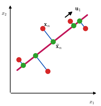
fig12_2. Download: PDF · SVG12.1.1 Maximum variance formulation
Fix \(M\lt D\) (choosing \(M\) is discussed in Section 12.2.3) and start with \(M=1\). A one-dimensional projection is described by a direction, which we take to be a unit vector \(\mathbf{u}_1\) (only the direction matters). The point \(\mathbf{x}_n\) is projected to the number \(\mathbf{u}_1^\T\mathbf{x}_n\). The projected data have mean \(\mathbf{u}_1^\T\bar{\mathbf{x}}\), where
\[ \bar{\mathbf{x}}=\frac1N\sum_{n=1}^N\mathbf{x}_n , \tag{12.1} \]and variance
\[ \frac1N\sum_{n=1}^N\big\{\mathbf{u}_1^\T\mathbf{x}_n-\mathbf{u}_1^\T\bar{\mathbf{x}}\big\}^2=\mathbf{u}_1^\T\mathbf{S}\mathbf{u}_1 , \tag{12.2} \] \[ \mathbf{S}=\frac1N\sum_{n=1}^N(\mathbf{x}_n-\bar{\mathbf{x}})(\mathbf{x}_n-\bar{\mathbf{x}})^\T . \tag{12.3} \]Maximising \(\mathbf{u}_1^\T\mathbf{S}\mathbf{u}_1\) without a constraint is pointless (it grows like \(\lVert\mathbf{u}_1\rVert^2\)), so we impose \(\mathbf{u}_1^\T\mathbf{u}_1=1\) with a Lagrange multiplier \(\lambda_1\) and look for stationary points of
\[ \mathbf{u}_1^\T\mathbf{S}\mathbf{u}_1+\lambda_1\big(1-\mathbf{u}_1^\T\mathbf{u}_1\big). \tag{12.4} \]They satisfy
\[ \mathbf{S}\mathbf{u}_1=\lambda_1\mathbf{u}_1 , \tag{12.5} \] \[ \mathbf{u}_1^\T\mathbf{S}\mathbf{u}_1=\lambda_1 . \tag{12.6} \]Filling the gap 12.1: from the projected variance to the eigenvector equation p. 562, (12.2)–(12.6)
The book states (12.2), differentiates (12.4) and concludes that the maximum is attained at the eigenvector with the largest eigenvalue. Here are the algebra of (12.2), the derivative, and the argument that the stationary point with the largest eigenvalue is the global maximum and not just a stationary point.
Derivation
The projected variance (12.2). Since \(\mathbf{u}_1^\T\mathbf{x}_n-\mathbf{u}_1^\T\bar{\mathbf{x}}\)
The stationarity condition (12.5). For a symmetric matrix, \(\nabla_{\mathbf{u}}(\mathbf{u}^\T\mathbf{S}\mathbf{u})\)
The global maximum. The unit sphere is closed and bounded and \(\mathbf{u}^\T\mathbf{S}\mathbf{u}\) is continuous, so a maximiser exists. It is a stationary point, hence a unit eigenvector, and its value is its eigenvalue; the best possible value is therefore the largest eigenvalue \(\lambda_1\). The same conclusion follows directly by expanding \(\mathbf{u}=\sum_i c_i\mathbf{u}_i\) in the orthonormal eigenbasis, so that \(\sum_ic_i^2=1\) and
\[ \mathbf{u}^\T\mathbf{S}\mathbf{u}=\sum_{i=1}^D\lambda_ic_i^2\le\lambda_1\sum_{i=1}^Dc_i^2=\lambda_1 , \]with equality exactly when \(c_i=0\) for every \(i\) with \(\lambda_i\lt\lambda_1\). If \(\lambda_1\gt\lambda_2\), the maximiser is \(\pm\mathbf{u}_1\) and nothing else. This is the Rayleigh quotient bound of the toolkit. The other eigenvectors are stationary points that are not maxima: along \(\mathbf{u}_i\) with \(1\lt i\lt D\) the variance can be increased by tilting towards \(\mathbf{u}_1\) and decreased by tilting towards \(\mathbf{u}_D\). ∎
Result 12.1 (the first principal component)
Over all unit vectors \(\mathbf{u}\), the projected variance \(\mathbf{u}^\T\mathbf{S}\mathbf{u}\) is maximised by the eigenvector \(\mathbf{u}_1\) of the largest eigenvalue, and the maximal variance is \(\lambda_1\). The maximiser is unique up to sign when \(\lambda_1\gt\lambda_2\).
Further directions are defined one at a time: each new direction maximises the projected variance among all unit vectors orthogonal to the directions already chosen. The book states that the resulting \(M\) directions are the eigenvectors of the \(M\) largest eigenvalues, "easily shown using proof by induction" (Exercise 12.1). Two statements are hidden in this sentence, and both are proved below: the one-at-a-time construction picks the eigenvectors in order, and the \(M\)-dimensional subspace so obtained maximises the total projected variance among all \(M\)-dimensional projections, not only among those built greedily.
Result 12.2 (maximum variance in \(M\) dimensions)
(a) One direction at a time (Exercise 12.1). If \(\mathbf{u}_1,\dots,\mathbf{u}_k\) are the first \(k\) principal components, then the unit vector orthogonal to all of them with the largest projected variance is \(\mathbf{u}_{k+1}\), and that variance is \(\lambda_{k+1}\).
(b) All directions at once (Ky Fan, 1949). For every \(D\times M\) matrix \(\mathbf{V}\) with orthonormal columns, the total variance of the projected data satisfies
\[ \frac1N\sum_{n=1}^N\big\lVert\mathbf{V}^\T(\mathbf{x}_n-\bar{\mathbf{x}})\big\rVert^2=\Tr(\mathbf{V}^\T\mathbf{S}\mathbf{V})\le\lambda_1+\dots+\lambda_M , \]with equality when the columns of \(\mathbf{V}\) span \(\operatorname{span}\{\mathbf{u}_1,\dots,\mathbf{u}_M\}\) (and only then, if \(\lambda_M\gt\lambda_{M+1}\)).
Proof
(a), with Lagrange multipliers as the exercise asks. Suppose, as induction hypothesis, that the first \(k\) directions are the eigenvectors \(\mathbf{u}_1,\dots,\mathbf{u}_k\) (true for \(k=1\) by Result 12.1). The next direction \(\mathbf{u}\) maximises \(\mathbf{u}^\T\mathbf{S}\mathbf{u}\) subject to \(\mathbf{u}^\T\mathbf{u}=1\) and \(\mathbf{u}^\T\mathbf{u}_j=0\) for \(j=1,\dots,k\). With multipliers \(\lambda\) and \(\eta_1,\dots,\eta_k\), the Lagrangian is
\[ \mathbf{u}^\T\mathbf{S}\mathbf{u}+\lambda\big(1-\mathbf{u}^\T\mathbf{u}\big)+\sum_{j=1}^k\eta_j\,\mathbf{u}^\T\mathbf{u}_j , \]and its gradient vanishes when \(2\mathbf{S}\mathbf{u}-2\lambda\mathbf{u}+\sum_j\eta_j\mathbf{u}_j\)
(b). The identity on the left is the computation of (12.2) applied to each column of \(\mathbf{V}\). Write \(\mathbf{S}\)
\(\mathbf{P}=\mathbf{V}\mathbf{V}^\T\) is the orthogonal projection onto the column space of \(\mathbf{V}\), so \(0\)
If the columns of \(\mathbf{V}\) span \(\operatorname{span}\{\mathbf{u}_1,\dots,\mathbf{u}_M\}\), then \(p_i=1\) for \(i\le M\) and \(p_i=0\) otherwise, and equality holds. Conversely, if \(\lambda_M\gt\lambda_{M+1}\), equality in the second step forces \(p_i=0\) for every \(i\gt M\) (and then \(p_i=1\) for \(i\le M\)), that is, the column space of \(\mathbf{V}\) is \(\operatorname{span}\{\mathbf{u}_1,\dots,\mathbf{u}_M\}\). Since the greedy directions of (a) attain the bound, they are also optimal among all \(M\)-dimensional projections. This is the "Ky Fan" form of the Rayleigh–Ritz theorem. ∎
In summary, PCA computes \(\bar{\mathbf{x}}\) and \(\mathbf{S}\) and finds the eigenvectors of the \(M\) largest eigenvalues. A full eigendecomposition of a \(D\times D\) matrix costs \(O(D^3)\); when only \(M\) eigenpairs are needed, iterative methods such as the power method cost \(O(MD^2)\) (Golub and Van Loan, 1996), and the EM algorithm of Section 12.2.2 avoids forming \(\mathbf{S}\) altogether. The power method itself is a one-line consequence of the eigen-expansion: \(\mathbf{S}^t\mathbf{v}\)
Algorithm 12.1 (principal component analysis)
- Compute the mean \(\bar{\mathbf{x}}\) (12.1) and the covariance \(\mathbf{S}\) (12.3); if \(N\lt D\) use the \(N\times N\) route of Result 12.5 instead.
- Find the eigenvectors \(\mathbf{u}_1,\dots,\mathbf{u}_M\) of the \(M\) largest eigenvalues \(\lambda_1\ge\dots\ge\lambda_M\) (or, equivalently, the leading right singular vectors of \(\widetilde{\mathbf{X}}\), with \(\lambda_i=\sigma_i^2/N\); toolkit).
- Scores: \(z_{ni}\)
\({}=\mathbf{u}_i^\T(\mathbf{x}_n-\bar{\mathbf{x}})\), \(i=1,\dots,M\). Reconstruction: \(\widetilde{\mathbf{x}}_n\) \({}=\bar{\mathbf{x}}+\sum_{i\le M}z_{ni}\mathbf{u}_i\) (12.20). - Retained variance \(\sum_{i\le M}\lambda_i\); mean squared reconstruction error \(J=\sum_{i\gt M}\lambda_i\) (12.18).
12.1.2 Minimum-error formulation
Now take any complete orthonormal basis \(\{\mathbf{u}_i\}_{i=1}^D\) of \(\R^D\),
\[ \mathbf{u}_i^\T\mathbf{u}_j=\delta_{ij} . \tag{12.7} \]Every data point has an exact expansion
\[ \mathbf{x}_n=\sum_{i=1}^D\alpha_{ni}\mathbf{u}_i , \tag{12.8} \]and taking the inner product with \(\mathbf{u}_j\) gives \(\alpha_{nj}\)
This is just a rotation of the coordinate system. To reduce the dimension we approximate \(\mathbf{x}_n\) using only \(M\) coefficients that depend on \(n\), the remaining \(D-M\) coefficients being constants \(b_i\) shared by all points:
\[ \widetilde{\mathbf{x}}_n=\sum_{i=1}^Mz_{ni}\mathbf{u}_i+\sum_{i=M+1}^Db_i\mathbf{u}_i . \tag{12.10} \](This is the general approximation by a point of an \(M\)-dimensional affine subspace: choose the basis so that \(\mathbf{u}_1,\dots,\mathbf{u}_M\) span the direction of the subspace; the offset is \(\sum_{i\gt M}b_i\mathbf{u}_i\).) The distortion is the mean squared error
\[ J=\frac1N\sum_{n=1}^N\lVert\mathbf{x}_n-\widetilde{\mathbf{x}}_n\rVert^2 . \tag{12.11} \]Minimising over the coefficients and the offsets gives (Bishop, p. 564; derivation below)
\[ z_{nj}=\mathbf{x}_n^\T\mathbf{u}_j\quad(j=1,\dots,M), \tag{12.12} \] \[ b_j=\bar{\mathbf{x}}^\T\mathbf{u}_j\quad(j=M+1,\dots,D), \tag{12.13} \] \[ \mathbf{x}_n-\widetilde{\mathbf{x}}_n=\sum_{i=M+1}^D\big\{(\mathbf{x}_n-\bar{\mathbf{x}})^\T\mathbf{u}_i\big\}\mathbf{u}_i , \tag{12.14} \] \[ J=\frac1N\sum_{n=1}^N\sum_{i=M+1}^D\big(\mathbf{x}_n^\T\mathbf{u}_i-\bar{\mathbf{x}}^\T\mathbf{u}_i\big)^2=\sum_{i=M+1}^D\mathbf{u}_i^\T\mathbf{S}\mathbf{u}_i . \tag{12.15} \]Filling the gap 12.2: the optimal coefficients and the distortion p. 564, (12.12)–(12.15)
The book says "setting the derivative ... to zero, and making use of the orthonormality conditions". The point is that orthonormality makes \(J\) a sum of independent one-dimensional least-squares problems.
Derivation
By (12.9) and (12.10),
\[ \mathbf{x}_n-\widetilde{\mathbf{x}}_n=\sum_{i=1}^M\big(\mathbf{x}_n^\T\mathbf{u}_i-z_{ni}\big)\mathbf{u}_i+\sum_{i=M+1}^D\big(\mathbf{x}_n^\T\mathbf{u}_i-b_i\big)\mathbf{u}_i . \]For orthonormal vectors, \(\lVert\sum_ic_i\mathbf{u}_i\rVert^2\)
Each \(z_{nj}\) appears in exactly one square, and \(\partial J/\partial z_{nj}\)
which is (12.14). Using Pythagoras again and the computation of (12.2) for each \(i\gt M\),
\[ J=\frac1N\sum_{n}\sum_{i\gt M}\big\{\mathbf{u}_i^\T(\mathbf{x}_n-\bar{\mathbf{x}})\big\}^2=\sum_{i\gt M}\mathbf{u}_i^\T\mathbf{S}\mathbf{u}_i , \]which is (12.15). Geometrically, (12.14) says the error vector is orthogonal to the subspace: within a fixed affine subspace the closest point is the orthogonal projection, and the best offset puts the subspace through \(\bar{\mathbf{x}}\) (the minimiser of \(\sum_n\lVert\mathbf{x}_n-\mathbf{c}\rVert^2\) over the discarded coordinates). ∎
It remains to choose the basis. For \(D=2\), \(M=1\) we must choose a unit vector \(\mathbf{u}_2\) minimising \(J\)
is stationary when \(\mathbf{S}\mathbf{u}_2\)
with distortion equal to the sum of the discarded eigenvalues,
\[ J=\sum_{i=M+1}^D\lambda_i . \tag{12.18} \]Result 12.3 (minimum-error PCA; the two definitions agree)
Over all orthonormal bases and all coefficients in (12.10), the smallest distortion is \(J_{\min}=\sum_{i\gt M}\lambda_i\). It is attained exactly when \(\operatorname{span}\{\mathbf{u}_1,\dots,\mathbf{u}_M\}\) is a principal subspace (Definition 12.1); the eigenvector basis (12.17) is one convenient choice, and any orthonormal basis of the principal subspace gives the same \(J\). Moreover, for every orthonormal basis,
\[ \underbrace{\sum_{i=1}^M\mathbf{u}_i^\T\mathbf{S}\mathbf{u}_i}_{\text{variance kept}}+\underbrace{\sum_{i=M+1}^D\mathbf{u}_i^\T\mathbf{S}\mathbf{u}_i}_{J\text{ (variance lost)}}=\Tr\mathbf{S}, \]so minimising the error and maximising the variance are the same problem.
Proof (Exercise 12.2, and a shortcut)
The identity. \(\sum_{i=1}^D\mathbf{u}_i^\T\mathbf{S}\mathbf{u}_i\)
Lagrangian with a matrix of multipliers. Put the discarded vectors into the \(D\times(D-M)\) matrix \(\widehat{\mathbf{U}}\)
\(\mathbf{H}\) may be taken symmetric. The matrix \(\mathbf{B}\)
Stationarity. With \(\partial\Tr(\mathbf{A}^\T\mathbf{S}\mathbf{A})/\partial\mathbf{A}\)
All stationary points. Diagonalise the symmetric \(\mathbf{H}\)
the sum of the eigenvalues of those \(D-M\) eigenvectors. The particular solution with \(\bm{\Psi}=\mathbf{I}\) (\(\mathbf{H}\) diagonal) has the eigenvectors themselves as columns; every other stationary point with the same subspace gives the same \(J\), which is why the book may "choose the eigenvector solution".
The minimum. The feasible set \(\{\widehat{\mathbf{U}}:\widehat{\mathbf{U}}^\T\widehat{\mathbf{U}}\)
If \(M=D\) nothing is discarded and PCA is simply a rotation of the axes onto the eigenvectors. A related linear method, canonical correlation analysis (CCA; Hotelling, 1936; Bach and Jordan, 2002), works with two random vectors \(\mathbf{x}\) and \(\mathbf{y}\) and looks for pairs of directions \(\mathbf{a},\mathbf{b}\) whose projections are maximally correlated. Maximising \(\mathbf{a}^\T\mathbf{S}_{xy}\mathbf{b}\) subject to \(\mathbf{a}^\T\mathbf{S}_{xx}\mathbf{a}\)
12.1.3 Applications of PCA
Compression of digit images
Take the 1010 images of the digit three in the MNIST test set (the book's "off-line digits" are MNIST, Appendix A); each is a vector of \(D=28\times28=784\) grey levels. Every eigenvector of \(\mathbf{S}\) is itself a vector in \(\R^{784}\) and can be shown as an image (Figure 12.3). Figure 12.4 shows the eigenvalue spectrum and the distortion \(J\) as a function of \(M\), which by (12.18) is the tail sum of the spectrum. With grey levels 0 to 255, as in the book, the first four eigenvalues are \(3.42\), \(2.80\), \(2.38\) and \(1.61\times10^5\), matching the book's \(3.4\), \(2.8\), \(2.4\) and \(1.6\times10^5\) (the 6131 threes of the training set give \(3.64\), \(2.71\), \(2.32\) and \(1.60\times10^5\), so the test set is the better match). In our computation, keeping \(M=1\), 10, 50 and 250 components retains 12.1%, 54.7%, 85.4% and 99.0% of the total variance \(\Tr\mathbf{S}\). Since 254 of the 784 pixels are blank in every one of these images, at least 254 eigenvalues are exactly zero. (Errata: the captions of Figures 12.3 and 12.4 should say "digit three", and the text on p. 566 shows the first four, not five, eigenvectors.)
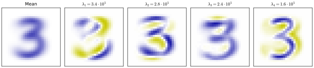
fig12_3. Download: PDF · SVG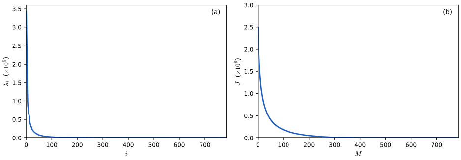
fig12_4. Download: PDF · SVGSubstituting (12.12) and (12.13) into (12.10), the PCA approximation of \(\mathbf{x}_n\) is
\[ \begin{aligned}\widetilde{\mathbf{x}}_n&=\sum_{i=1}^M\big(\mathbf{x}_n^\T\mathbf{u}_i\big)\mathbf{u}_i+\sum_{i=M+1}^D\big(\bar{\mathbf{x}}^\T\mathbf{u}_i\big)\mathbf{u}_i &(12.19)\\ &=\bar{\mathbf{x}}+\sum_{i=1}^M\big(\mathbf{x}_n^\T\mathbf{u}_i-\bar{\mathbf{x}}^\T\mathbf{u}_i\big)\mathbf{u}_i , &(12.20)\end{aligned} \]where the second line replaces \(\sum_{i\gt M}(\bar{\mathbf{x}}^\T\mathbf{u}_i)\mathbf{u}_i\) by \(\bar{\mathbf{x}}-\sum_{i\le M}(\bar{\mathbf{x}}^\T\mathbf{u}_i)\mathbf{u}_i\), using the expansion of the mean in the complete basis,
\[ \bar{\mathbf{x}}=\sum_{i=1}^D\big(\bar{\mathbf{x}}^\T\mathbf{u}_i\big)\mathbf{u}_i . \tag{12.21} \]This is a compression: once \(\bar{\mathbf{x}}\) and \(\mathbf{u}_1,\dots,\mathbf{u}_M\) are stored (\(D(M+1)\) numbers, shared by the whole data set), each image is described by the \(M\) scores \(\mathbf{x}_n^\T\mathbf{u}_i-\bar{\mathbf{x}}^\T\mathbf{u}_i\) instead of its \(D\) pixels. Figure 12.5 shows reconstructions for several \(M\).
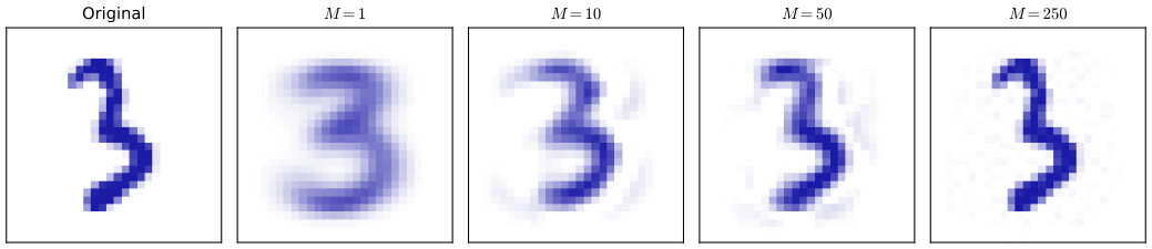
fig12_5. Download: PDF · SVGPre-processing: standardisation and whitening
PCA is also used to put data into a standard form before another algorithm is applied, for example when variables are measured in different units. In the Old Faithful data the waiting time is about an order of magnitude larger than the eruption duration, which is why Section 9.1 first standardised each variable to zero mean and unit variance. The covariance matrix of the standardised data is the correlation matrix
\[ \rho_{ij}=\frac1N\sum_{n=1}^N\frac{(x_{ni}-\bar{x}_i)}{\sigma_i}\frac{(x_{nj}-\bar{x}_j)}{\sigma_j} , \tag{12.22} \]where \(\sigma_i\) is the standard deviation of variable \(i\) (computed with divisor \(N\); erratum: the first printing says "variance"). It has \(\rho_{ii}=1\) and \(\lvert\rho_{ij}\rvert\le1\) (Cauchy–Schwarz), with \(\rho_{ij}=\pm1\) for perfectly (linearly) correlated variables and 0 for uncorrelated ones. Standardisation rescales the variables but does not remove their correlation. PCA can do more: write the eigenvector equations (12.17) together as
\[ \mathbf{S}\mathbf{U}=\mathbf{U}\mathbf{L} , \tag{12.23} \]with \(\mathbf{L}\)
Result 12.4 (whitening)
If all eigenvalues of \(\mathbf{S}\) are positive, the whitened points (12.24) have sample mean \(\mathbf{0}\) and sample covariance \(\mathbf{I}\):
\[ \frac1N\sum_{n=1}^N\mathbf{y}_n\mathbf{y}_n^\T=\frac1N\sum_{n=1}^N\mathbf{L}^{-1/2}\mathbf{U}^\T(\mathbf{x}_n-\bar{\mathbf{x}})(\mathbf{x}_n-\bar{\mathbf{x}})^\T\mathbf{U}\mathbf{L}^{-1/2}=\mathbf{L}^{-1/2}\mathbf{U}^\T\mathbf{S}\mathbf{U}\mathbf{L}^{-1/2}=\mathbf{L}^{-1/2}\mathbf{L}\mathbf{L}^{-1/2}=\mathbf{I}. \tag{12.25} \]Euclidean distances between whitened points are Mahalanobis distances between the original points: \(\lVert\mathbf{y}_n-\mathbf{y}_m\rVert^2\)
Proof
Mean. The map (12.24) is affine, so \(\frac1N\sum_n\mathbf{y}_n\)
Covariance. The first equality in (12.25) is the definition of \(\mathbf{y}_n\) (note \((\mathbf{L}^{-1/2})^\T\)
Distances. \(\mathbf{y}_n-\mathbf{y}_m\)
Two remarks. Whitening is not unique: for any orthogonal \(\mathbf{Q}\), the points \(\mathbf{Q}\mathbf{y}_n\) are white too, since their covariance is \(\mathbf{Q}\mathbf{I}\mathbf{Q}^\T\)
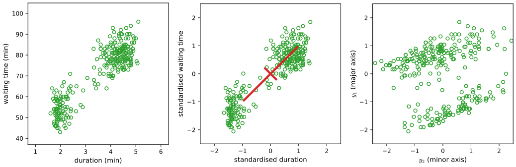
fig12_6. Download: PDF · SVGPCA versus Fisher's linear discriminant
Both PCA and Fisher's linear discriminant (Section 4.1.4) reduce the dimension linearly, but PCA is unsupervised: it sees only the \(\mathbf{x}_n\). Fisher's discriminant also uses the class labels, and the two can disagree badly (Figure 12.7).
Filling the gap 12.3: why PCA can mix the classes p. 568, Figure 12.7
The book makes the comparison through a picture. The algebra: for two classes, the total covariance splits into a within-class part and a between-class part, and PCA maximises their sum while Fisher maximises their ratio.
Derivation
Let class \(\mathcal{C}_k\) have \(N_k\) points and mean \(\mathbf{m}_k\) (\(N_1+N_2=N\)), let \(\mathbf{S}_W\)
because \(\bar{\mathbf{x}}\)
PCA rewards within-class spread exactly as much as separation of the means. If the classes are elongated along a common direction that does not separate them (Figure 12.7), the within-class term dominates and PCA picks that direction, projecting both classes onto the same interval. Fisher's criterion (4.26) penalises within-class spread and is maximised by \(\mathbf{u}\propto\mathbf{S}_W^{-1}\mathbf{d}\) (4.30). ∎
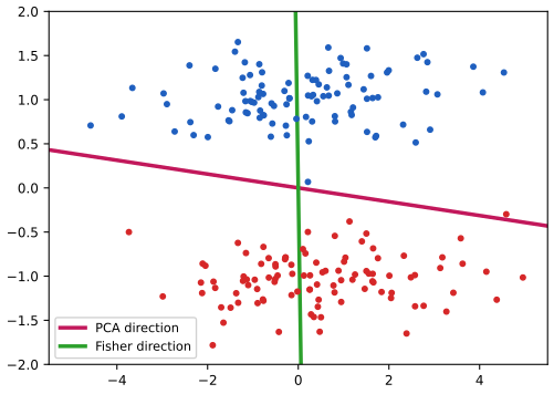
fig12_7. Download: PDF · SVGVisualisation
For visualisation one takes \(M=2\) and plots each point at the coordinates \((\mathbf{x}_n^\T\mathbf{u}_1,\mathbf{x}_n^\T\mathbf{u}_2)\) (or the centred scores, which only shifts the picture). Figure 12.8 does this for the oil flow data.
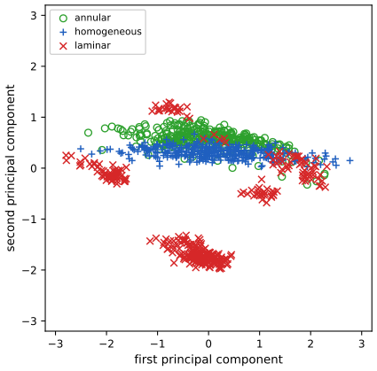
fig12_8. Download: PDF · SVG12.1.4 PCA for high-dimensional data
Sometimes \(N\lt D\): a few hundred images, each with millions of pixels. Then \(N\) points span an affine subspace of dimension at most \(N-1\), so at least \(D-N+1\) eigenvalues of \(\mathbf{S}\) are zero and components beyond \(N-1\) are meaningless; worse, an \(O(D^3)\) eigendecomposition is out of reach. The remedy works with the centred \(N\times D\) data matrix \(\mathbf{X}\) (rows \((\mathbf{x}_n-\bar{\mathbf{x}})^\T\)), for which \(\mathbf{S}\)
Multiplying by \(\mathbf{X}\),
\[ \frac1N\mathbf{X}\mathbf{X}^\T(\mathbf{X}\mathbf{u}_i)=\lambda_i(\mathbf{X}\mathbf{u}_i) , \tag{12.27} \]so \(\mathbf{v}_i\)
Conversely, multiplying (12.28) by \(\mathbf{X}^\T\),
\[ \frac1N\mathbf{X}^\T\mathbf{X}(\mathbf{X}^\T\mathbf{v}_i)=\lambda_i(\mathbf{X}^\T\mathbf{v}_i) , \tag{12.29} \]so \(\mathbf{X}^\T\mathbf{v}_i\) is an eigenvector of \(\mathbf{S}\), and if \(\lVert\mathbf{v}_i\rVert=1\) the unit eigenvector is
\[ \mathbf{u}_i=\frac{1}{(N\lambda_i)^{1/2}}\mathbf{X}^\T\mathbf{v}_i . \tag{12.30} \]Result 12.5 (PCA through the \(N\times N\) matrix)
(a) \(\operatorname{rank}\mathbf{X}\)
Proof
(a) The rows of \(\mathbf{X}\) sum to zero, \(\mathbf{1}^\T\mathbf{X}\)
(b) Let \(\lambda\ne0\) be an eigenvalue of \(N^{-1}\mathbf{X}^\T\mathbf{X}\) with eigenspace \(E\). For \(\mathbf{u}\in E\setminus\{\mathbf{0}\}\), (12.27) shows that \(\mathbf{X}\mathbf{u}\) is an eigenvector of \(N^{-1}\mathbf{X}\mathbf{X}^\T\) with eigenvalue \(\lambda\), and \(\mathbf{X}\mathbf{u}\ne\mathbf{0}\) because \(\mathbf{X}^\T(\mathbf{X}\mathbf{u})\)
(c) By (12.29) each \(\mathbf{u}_i\) is an eigenvector of \(\mathbf{S}\) with eigenvalue \(\lambda_i\). For the inner products, use (12.28) in the form \(\mathbf{X}\mathbf{X}^\T\mathbf{v}_j\)
In particular \(\lVert\mathbf{X}^\T\mathbf{v}_i\rVert^2\)
This "snapshot" trick (Sirovich, 1987) reappears in kernel PCA (Section 12.3), where the feature space may be infinite-dimensional and only the \(N\times N\) matrix of inner products is available.
12.2 Probabilistic PCA
So far PCA is a projection with no probability model behind it. This section shows that it is the maximum likelihood solution of a simple latent variable model, probabilistic PCA (PPCA), proposed independently by Tipping and Bishop (1997, 1999b) and by Roweis (1998), and closely related to factor analysis (Section 12.2.4). Having a model brings several things that plain PCA lacks (Bishop, pp. 570–571):
- a Gaussian density whose number of free parameters can be controlled while it still captures the dominant correlations (Result 12.10);
- EM algorithms that need only a few leading eigenvectors, never form \(\mathbf{S}\), cope with missing values and extend to mixtures of PCA models (Sections 12.2.2 and 12.4.3);
- a likelihood, and therefore Bayesian methods that choose the dimension \(M\) automatically (Section 12.2.3), and comparison with other density models: PCA gives a small reconstruction error to any point near the principal subspace, even one far away from all the data, whereas the PPCA density is small there;
- class-conditional densities for classifiers, and samples from the fitted distribution.
Definition 12.2 (probabilistic PCA)
An \(M\)-dimensional latent variable \(\mathbf{z}\) has a standard Gaussian prior, and given \(\mathbf{z}\) the observation is Gaussian with mean linear in \(\mathbf{z}\) and isotropic covariance:
\[ p(\mathbf{z})=\N(\mathbf{z}\given\mathbf{0},\mathbf{I}), \tag{12.31} \] \[ p(\mathbf{x}\given\mathbf{z})=\N(\mathbf{x}\given\mathbf{W}\mathbf{z}+\bm{\mu},\sigma^2\mathbf{I}). \tag{12.32} \]The parameters are the \(D\times M\) matrix \(\mathbf{W}\), the vector \(\bm{\mu}\in\R^D\) and the scalar \(\sigma^2\gt0\). Equivalently, as a generative recipe,
\[ \mathbf{x}=\mathbf{W}\mathbf{z}+\bm{\mu}+\bm{\epsilon}, \tag{12.33} \]with \(\mathbf{z}\sim\N(\mathbf{0},\mathbf{I}_M)\) and noise \(\bm{\epsilon}\sim\N(\mathbf{0},\sigma^2\mathbf{I}_D)\) independent of \(\mathbf{z}\).
Writing \(\widetilde{\mathbf{w}}_d^\T\) for the \(d\)th row of \(\mathbf{W}\), (12.32) factorises as \(p(\mathbf{x}\given\mathbf{z})\)
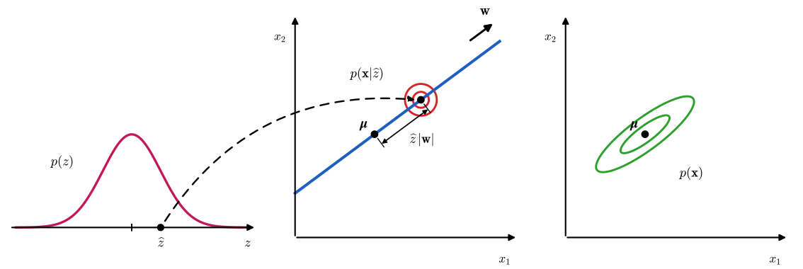
fig12_9. Download: PDF · SVGTo fit the model by maximum likelihood we need the marginal distribution of \(\mathbf{x}\),
\[ p(\mathbf{x})=\int p(\mathbf{x}\given\mathbf{z})\,p(\mathbf{z})\,\d\mathbf{z}. \tag{12.34} \]Because the model is linear-Gaussian, this is Gaussian (Exercise 12.7):
\[ p(\mathbf{x})=\N(\mathbf{x}\given\bm{\mu},\mathbf{C}), \tag{12.35} \] \[ \mathbf{C}=\mathbf{W}\mathbf{W}^\T+\sigma^2\mathbf{I}. \tag{12.36} \]Given that \(\mathbf{x}\) is Gaussian, its mean and covariance follow from (12.33) and the independence of \(\mathbf{z}\) and \(\bm{\epsilon}\) (so \(\E[\mathbf{z}\bm{\epsilon}^\T]\)
(It is Gaussian because \((\mathbf{z},\bm{\epsilon})\) is jointly Gaussian, being a pair of independent Gaussian vectors, and \(\mathbf{x}\) is an affine function of it; toolkit.) Bishop's picture: an isotropic Gaussian "spray can" moved across the principal subspace, spraying ink with density weighted by the prior, leaves a pancake-shaped density in data space.
The parametrisation is redundant. If \(\widetilde{\mathbf{W}}\)
so \(\mathbf{W}\) and \(\mathbf{W}\mathbf{R}\) define the same distribution of \(\mathbf{x}\): rotating the latent coordinates (\(\mathbf{z}\mapsto\mathbf{R}^\T\mathbf{z}\) leaves \(\N(\mathbf{0},\mathbf{I})\) unchanged) and counter-rotating \(\mathbf{W}\) changes nothing that can be observed. Evaluating the density requires \(\mathbf{C}^{-1}\), which the Woodbury identity reduces to an \(M\times M\) inversion:
\[ \mathbf{C}^{-1}=\sigma^{-2}\mathbf{I}-\sigma^{-2}\mathbf{W}\mathbf{M}^{-1}\mathbf{W}^\T , \tag{12.40} \] \[ \mathbf{M}=\mathbf{W}^\T\mathbf{W}+\sigma^2\mathbf{I}. \tag{12.41} \](Erratum: the first printing has \(\sigma^{-1}\mathbf{I}\) as the first term of (12.40).) The posterior distribution of the latent variable is
\[ p(\mathbf{z}\given\mathbf{x})=\N\big(\mathbf{z}\given\mathbf{M}^{-1}\mathbf{W}^\T(\mathbf{x}-\bm{\mu}),\,\sigma^2\mathbf{M}^{-1}\big) \tag{12.42} \](erratum: the first printing has \(\sigma^{-2}\mathbf{M}\) as the covariance). Its mean depends on \(\mathbf{x}\), its covariance does not.
Result 12.6 (marginal and posterior of probabilistic PCA)
For the model of Definition 12.2, with \(\mathbf{C}\) and \(\mathbf{M}\) as in (12.36) and (12.41): (a) the marginal of \(\mathbf{x}\) is (12.35); (b) \(\mathbf{C}^{-1}\) is given by (12.40), and \(\lvert\mathbf{C}\rvert\)
Proof (all four facts from one completion of the square)
The book obtains (12.35) from the general linear-Gaussian results (2.115) and (12.42) from (2.116) (Exercises 12.7 and 12.8; see the toolkit). Here everything is derived directly. The joint density is \(p(\mathbf{x}\given\mathbf{z})p(\mathbf{z})\)
The matrix of the quadratic form is \(\mathbf{I}+\sigma^{-2}\mathbf{W}^\T\mathbf{W}\)
(Expand the first term: \(\sigma^{-2}\{\mathbf{z}^\T\mathbf{M}\mathbf{z}-2\mathbf{z}^\T\mathbf{W}^\T\mathbf{y}+\mathbf{y}^\T\mathbf{W}\mathbf{M}^{-1}\mathbf{W}^\T\mathbf{y}\}\), so the last term of the second bracket cancels the extra piece.) (c): as a function of \(\mathbf{z}\), the joint density is proportional to \(\exp\{-\tfrac{1}{2\sigma^2}(\mathbf{z}-\mathbf{m})^\T\mathbf{M}(\mathbf{z}-\mathbf{m})\}\), a Gaussian with mean \(\mathbf{m}\) and covariance \(\sigma^2\mathbf{M}^{-1}\), which is (12.42). (b), first part: the second bracket is \(\mathbf{y}^\T\mathbf{A}\mathbf{y}\) with \(\mathbf{A}\)
(This is the Woodbury identity with \(\mathbf{A}=\sigma^2\mathbf{I}\), \(\mathbf{U}=\mathbf{W}\), \(\mathbf{V}=\mathbf{W}^\T\).) (a) and the determinant: integrating the Gaussian factor over \(\mathbf{z}\) gives \((2\pi)^{M/2}\lvert\sigma^2\mathbf{M}^{-1}\rvert^{1/2}\)
This is a Gaussian with mean \(\bm{\mu}\) and covariance \(\mathbf{C}\), provided the constant equals \((2\pi)^{-D/2}\lvert\mathbf{C}\rvert^{-1/2}\), that is \(\lvert\mathbf{C}\rvert\)
12.2.1 Maximum likelihood PCA
For independent observations \(\mathbf{X}=\{\mathbf{x}_n\}\), (12.35) gives the log likelihood
\[ \ln p(\mathbf{X}\given\bm{\mu},\mathbf{W},\sigma^2)=\sum_{n=1}^N\ln p(\mathbf{x}_n\given\mathbf{W},\bm{\mu},\sigma^2)=-\frac{ND}{2}\ln(2\pi)-\frac N2\ln\lvert\mathbf{C}\rvert-\frac12\sum_{n=1}^N(\mathbf{x}_n-\bm{\mu})^\T\mathbf{C}^{-1}(\mathbf{x}_n-\bm{\mu}). \tag{12.43} \]Maximising over \(\bm{\mu}\) gives \(\bm{\mu}_{\rm ML}=\bar{\mathbf{x}}\), and substituting back,
\[ \ln p(\mathbf{X}\given\mathbf{W},\bm{\mu},\sigma^2)=-\frac N2\Big\{D\ln(2\pi)+\ln\lvert\mathbf{C}\rvert+\Tr\big(\mathbf{C}^{-1}\mathbf{S}\big)\Big\}. \tag{12.44} \]Result 12.7 (the mean; Exercises 12.9 and 12.10)
For any fixed \(\mathbf{W}\) and \(\sigma^2\gt0\), (12.43) is a strictly concave quadratic function of \(\bm{\mu}\) with unique maximiser \(\bm{\mu}=\bar{\mathbf{x}}\), and its maximised value is (12.44).
Proof
Only the last term of (12.43) involves \(\bm{\mu}\). Its gradient is \(\sum_n\mathbf{C}^{-1}(\mathbf{x}_n-\bm{\mu})\)
Collecting the factor \(-N/2\) gives (12.44). ∎
Maximisation over \(\mathbf{W}\) and \(\sigma^2\) is harder but still has a closed form. The book quotes it from Tipping and Bishop (1999b): every stationary point has the form
\[ \mathbf{W}_{\rm ML}=\mathbf{U}_M(\mathbf{L}_M-\sigma^2\mathbf{I})^{1/2}\mathbf{R}, \tag{12.45} \]where the columns of \(\mathbf{U}_M\) are any \(M\) eigenvectors of \(\mathbf{S}\), \(\mathbf{L}_M\) is the diagonal matrix of their eigenvalues and \(\mathbf{R}\) is an arbitrary \(M\times M\) orthogonal matrix; the maximum is attained when the eigenvectors are those of the \(M\) largest eigenvalues (all other choices being saddle points), and then
\[ \sigma^2_{\rm ML}=\frac{1}{D-M}\sum_{i=M+1}^D\lambda_i , \tag{12.46} \]the average variance of the discarded directions. The book gives no proof; the next result supplies it.
Result 12.8 (maximum likelihood probabilistic PCA; Tipping and Bishop, 1999b)
Assume \(\mathbf{S}\) has at least \(M+1\) positive eigenvalues (as it does when \(N\ge M+2\) and the data are in general position) and \(\lambda_M\gt\lambda_D\).
(a) Stationary points. \((\mathbf{W},\sigma^2)\) is a stationary point of (12.44) exactly when \(\mathbf{W}\)
(b) The maximum. The log likelihood attains its maximum, at (12.45) with \(\mathbf{U}_M\)
(c) Saddle points. Every stationary point that uses a non-principal eigenvector (one whose eigenvalue is smaller than that of an unused eigenvector) or has a zero column is a saddle point, unless the unused eigenvalues are all equal.
Proof (the full Tipping–Bishop argument, with the existence of the maximum added)
Write \(\mathcal{L}(\mathbf{W},\sigma^2)\) for (12.44).
Step 1: the gradient and the stationarity condition. With \(\d\ln\lvert\mathbf{C}\rvert\)
Since \(\d f\)
Multiplying the first by \(\mathbf{C}/N\), the stationarity condition in \(\mathbf{W}\) is
\[ \mathbf{S}\mathbf{C}^{-1}\mathbf{W}=\mathbf{W}. \]Tipping and Bishop distinguish three kinds of solution: (i) \(\mathbf{W}=\mathbf{0}\), which satisfies it trivially; (ii) \(\mathbf{C}=\mathbf{S}\), the case of an exact covariance model, possible only when \(\mathbf{S}-\sigma^2\mathbf{I}\) is positive semi-definite of rank at most \(M\), i.e. when the \(D-M\) smallest eigenvalues of \(\mathbf{S}\) all equal \(\sigma^2\); (iii) \(\mathbf{W}\ne\mathbf{0}\) and \(\mathbf{C}\ne\mathbf{S}\), the generic case. The singular value decomposition handles all three at once.
Step 2: the singular value decomposition of \(\mathbf{W}\). Write \(\mathbf{W}\)
The stationarity condition becomes \(\mathbf{S}\mathbf{U}\mathbf{L}(\mathbf{L}^2+\sigma^2\mathbf{I})^{-1}\mathbf{V}^\T\)
So either \(l_j=0\) (the \(j\)th column of \(\mathbf{W}\mathbf{V}\) vanishes and \(\mathbf{u}_j'\) is unconstrained), or \(\mathbf{u}_j'\) is an eigenvector of \(\mathbf{S}\) whose eigenvalue \(\lambda\) satisfies \(\lambda=\sigma^2+l_j^2\), i.e. \(l_j=(\lambda-\sigma^2)^{1/2}\), which requires \(\lambda\gt\sigma^2\). Setting \(k_j=\sigma^2+l_j^2\) and \(\mathbf{R}=\mathbf{V}^\T\) gives \(\mathbf{W}\)
Step 3: the noise variance. Fix a stationary \(\mathbf{W}\) whose \(q\) non-zero columns use the eigenvectors \(\mathbf{u}_j\), \(j\in\mathcal{I}\) (\(\lvert\mathcal{I}\rvert=q\le M\)). Then \(\mathbf{C}\)
As a function of \(\sigma^2\) this has the form \(-\tfrac N2\{a\ln\sigma^2+b/\sigma^2\}+\const\) with \(a=D-q\gt0\), \(b\)
the average of the eigenvalues not used, which for \(q=M\) and \(\mathcal{I}=\{1,\dots,M\}\) is (12.46). (The same equation comes from \(\partial\mathcal{L}/\partial\sigma^2\)
which with \(\mathcal{I}=\{1,\dots,M\}\) is the maximal value stated in (b).
Step 4: zero columns are not maxima. Suppose \(q\lt M\), so \(\mathbf{W}\) (after the rotation \(\mathbf{R}\)) has a zero column, and let \(\mathbf{u}_i\), \(i\notin\mathcal{I}\), be an unused eigenvector. Put \(\varepsilon\mathbf{u}_i\) into the zero column. Then \(\mathbf{C}_\varepsilon\)
which is positive for small \(\varepsilon\) whenever \(\lambda_i\gt\sigma^2\). Because \(\sigma^2\) is the average of the unused eigenvalues, one of them exceeds it unless they are all equal. So such a point is not a local maximum; in particular \(\mathbf{W}=\mathbf{0}\) (with \(\sigma^2=\Tr\mathbf{S}/D\)) is not a maximum unless \(\mathbf{S}\propto\mathbf{I}\).
Step 5: non-principal eigenvectors give saddle points. Suppose that at a stationary point (any \(q\)) a used eigenvector \(\mathbf{u}_j\) (\(j\in\mathcal{I}\)) has a smaller eigenvalue than an unused one \(\mathbf{u}_i\) (\(i\notin\mathcal{I}\)): \(\lambda_i\gt\lambda_j\). Rotate in the plane of these two vectors: let \(\mathbf{Q}_\theta\) map \(\mathbf{u}_j\mapsto\cos\theta\,\mathbf{u}_j+\sin\theta\,\mathbf{u}_i\), \(\mathbf{u}_i\mapsto\cos\theta\,\mathbf{u}_i-\sin\theta\,\mathbf{u}_j\) and fix every other eigenvector, and move to \(\mathbf{W}(\theta)\)
Only \(k=i,j\) change: \((\mathbf{Q}_\theta\mathbf{u}_j)^\T\mathbf{S}(\mathbf{Q}_\theta\mathbf{u}_j)\)
because \(\lambda_i\gt\lambda_j\gt\sigma^2\). In the opposite direction, changing only the length of column \(j\) changes only the eigenvalue \(c=\sigma^2+l_j^2\) of \(\mathbf{C}\) along \(\mathbf{u}_j\), and \(-\tfrac2N\mathcal{L}\) changes by \(\ln c+\lambda_j/c\), which is minimal at \(c=\lambda_j\): the likelihood decreases. A point that is a maximum along one direction and a minimum along another is a saddle point. (The rotation is also "pure": the likelihood is flat along the \(M(M-1)/2\) directions \(\mathbf{W}\mapsto\mathbf{W}\mathbf{R}\).)
Step 6: the maximum exists. For any \(\mathbf{W}\), \(\mathbf{C}\) has eigenvalue \(\sigma^2\) on the orthogonal complement of the column space of \(\mathbf{W}\); let \(\mathbf{P}\) be the orthogonal projection onto that complement (rank at least \(D-M\)). Then \(\mathbf{C}^{-1}-\sigma^{-2}\mathbf{P}\) is positive semi-definite, so \(\Tr(\mathbf{C}^{-1}\mathbf{S})\)
with \(\sigma^2_{\rm ML}\gt0\) by the assumption on the rank. The right side tends to \(+\infty\) as \(\sigma^2\to0\) or \(\sigma^2\to\infty\), and for \(\sigma^2\) in a closed interval inside \((0,\infty)\) the second lower bound on \(\ln\lvert\mathbf{C}\rvert\) tends to \(+\infty\) as \(\lVert\mathbf{W}\rVert\to\infty\). So the sets \(\{\mathcal{L}\ge c\}\) are closed and bounded, \(\mathcal{L}\) attains its maximum, and the maximiser is a stationary point.
Conclusion. By Step 5 the maximiser has no unused eigenvalue larger than a used one, so it uses the eigenvectors of the \(q\) largest eigenvalues. If \(q\lt M\), Step 4 would force \(\lambda_{q+1}=\dots=\lambda_D\), hence \(\lambda_M=\lambda_D\), contrary to the assumption; so \(q=M\), the eigenvectors are \(\mathbf{u}_1,\dots,\mathbf{u}_M\) (and \(\lambda_M\gt\sigma^2_{\rm ML}\), as required for real \(l_j\), again because \(\lambda_M\gt\lambda_D\)), and by Step 3 the noise variance is (12.46). All such points have the same likelihood: they differ only by \(\mathbf{R}\) and, if \(\lambda_M=\lambda_{M+1}\), by the choice of eigenvectors in the tied eigenspace. ∎
A complementary view compares the stationary values directly. If the top \(q\) eigenvectors are used, Step 3 gives \(-\tfrac2N\mathcal{L}\)
Interpretation. Take \(\mathbf{R}=\mathbf{I}\): the columns of \(\mathbf{W}_{\rm ML}\) are the principal eigenvectors scaled by \((\lambda_i-\sigma^2)^{1/2}\). (Erratum: the first printing omits "square root of" in this sentence on p. 575.) Variances of independent contributions add, so along \(\mathbf{u}_i\) the data variance \(\lambda_i\) is split into \(\lambda_i-\sigma^2\) from the latent variable (pushed through the \(i\)th column of \(\mathbf{W}\)) and \(\sigma^2\) from the noise. For a unit vector \(\mathbf{v}\), the model variance is \(\mathbf{v}^\T\mathbf{C}\mathbf{v}\): if \(\mathbf{v}\) is orthogonal to the principal subspace (\(\mathbf{v}^\T\mathbf{U}_M\)
If the maximum likelihood solution is found by numerical optimisation (for example conjugate gradients) or by EM, \(\mathbf{R}\) is essentially arbitrary and the columns of \(\mathbf{W}\) need not be orthogonal. The principal axes are easy to recover: \(\mathbf{W}^\T\mathbf{W}\)
With \(M=D\) there is no reduction: \(\mathbf{U}_M=\mathbf{U}\), \(\mathbf{L}_M=\mathbf{L}\), and \(\mathbf{U}\mathbf{U}^\T\)
the unrestricted Gaussian maximum likelihood estimate (any \(\sigma^2\le\lambda_D\) then gives the same \(\mathbf{C}\), so \(\sigma^2\) is no longer determined).
From the data space back to the latent space
For visualisation and compression we reverse the mapping with Bayes' theorem and summarise a point \(\mathbf{x}\) by its posterior. From (12.42), the posterior mean is
\[ \E[\mathbf{z}\given\mathbf{x}]=\mathbf{M}^{-1}\mathbf{W}_{\rm ML}^\T(\mathbf{x}-\bar{\mathbf{x}}) , \tag{12.48} \]which corresponds to the point
\[ \mathbf{W}\E[\mathbf{z}\given\mathbf{x}]+\bm{\mu} \tag{12.49} \]in data space. As the book notes, this has the form of regularised linear regression (Section 3.3.1): \(\E[\mathbf{z}\given\mathbf{x}]\) minimises \(\lVert\mathbf{x}-\bm{\mu}-\mathbf{W}\mathbf{z}\rVert^2+\sigma^2\lVert\mathbf{z}\rVert^2\), whose normal equations are \((\mathbf{W}^\T\mathbf{W}+\sigma^2\mathbf{I})\mathbf{z}\)
an orthogonal projection onto the principal subspace, so standard PCA is recovered (Exercise 12.11); the posterior covariance tends to zero and the density becomes singular. For \(\sigma^2\gt0\) the projection is pulled towards the origin (Exercise 12.12).
Result 12.9 (posterior-mean projection and shrinkage; Exercises 12.11–12.13)
(a) For any full-rank \(\mathbf{W}\), let \(\mathbf{W}^\T\mathbf{W}\)
(b) At the maximum likelihood solution (12.45), (12.46) with \(\mathbf{R}=\mathbf{I}\),
\[ \mathbf{W}_{\rm ML}\E[\mathbf{z}\given\mathbf{x}]=\sum_{i=1}^M\frac{\lambda_i-\sigma^2}{\lambda_i}\,\big\{\mathbf{u}_i^\T(\mathbf{x}-\bar{\mathbf{x}})\big\}\,\mathbf{u}_i , \]while the orthogonal projection has factors 1: each principal score is shrunk by \((\lambda_i-\sigma^2)/\lambda_i\), most strongly in the directions with the least signal.
(c) The point of the principal subspace closest to \(\mathbf{x}\) can still be recovered from the posterior mean: it is \(\bar{\mathbf{x}}+\mathbf{W}_{\rm ML}(\mathbf{W}_{\rm ML}^\T\mathbf{W}_{\rm ML})^{-1}\mathbf{M}\,\E[\mathbf{z}\given\mathbf{x}]\), which is (12.94) of Exercise 12.13 (the book writes it for centred data, without \(\bar{\mathbf{x}}\)).
Proof
(a) \(\mathbf{M}\)
(b) With \(\mathbf{R}=\mathbf{I}\), \(\mathbf{W}_{\rm ML}^\T\mathbf{W}_{\rm ML}\)
(c) By (12.48), \(\mathbf{M}\E[\mathbf{z}\given\mathbf{x}]\)
How many parameters?
PPCA defines a Gaussian whose number of free parameters is controlled by \(M\). A full covariance has \(D(D+1)/2\) parameters (plus \(D\) for the mean), quadratic in \(D\); a diagonal one has \(D\) but cannot express correlations. PPCA keeps the \(M\) dominant correlations with a count that grows only linearly in \(D\). The matrix \(\mathbf{W}\) and \(\sigma^2\) have \(DM+1\) entries, but the rotation (12.39) makes some of them redundant. An \(M\times M\) orthogonal matrix has \(M-1\) free parameters in its first column (a unit vector), \(M-2\) in the second (unit and orthogonal to the first), and so on, \(M(M-1)/2\) in total. The number of degrees of freedom in \(\mathbf{C}\) is therefore
\[ DM+1-M(M-1)/2 . \tag{12.51} \]Result 12.10 (degrees of freedom of the PPCA covariance; Exercise 12.14)
For \(M\le D-1\), two matrices \(\mathbf{W}_1,\mathbf{W}_2\) of full column rank give the same \(\mathbf{W}\mathbf{W}^\T\) if and only if \(\mathbf{W}_2\)
Proof
If \(\mathbf{W}_1\mathbf{W}_1^\T\)
With \(M=D-1\), the columns of \(\mathbf{W}\) control the variance along \(D-1\) independent directions and \(\sigma^2\) the variance along the remaining one, so PPCA interpolates between the isotropic Gaussian (\(M=0\)) and the full-covariance Gaussian (\(M=D-1\)).
12.2.2 EM algorithm for PCA
PPCA has a latent \(\mathbf{z}_n\) for every \(\mathbf{x}_n\), so the general EM algorithm of Section 9.4 applies. With a closed-form maximum already available (Result 12.8) this may look pointless, but EM has real advantages: in high dimensions each iteration is cheaper than an eigendecomposition and never forms \(\mathbf{S}\); the same algorithm extends to factor analysis, which has no closed form (Section 12.2.4); and it handles missing data. Since the data points are independent, the complete-data log likelihood is
\[ \ln p\big(\mathbf{X},\mathbf{Z}\given\bm{\mu},\mathbf{W},\sigma^2\big)=\sum_{n=1}^N\big\{\ln p(\mathbf{x}_n\given\mathbf{z}_n)+\ln p(\mathbf{z}_n)\big\}, \tag{12.52} \]where the \(n\)th row of \(\mathbf{Z}\) is \(\mathbf{z}_n^\T\). We set \(\bm{\mu}=\bar{\mathbf{x}}\), its exact maximum likelihood value (Result 12.7). Taking the expectation with respect to the posterior of the latent variables gives
\[ \begin{aligned}\E\big[\ln p(\mathbf{X},\mathbf{Z}\given\bm{\mu},\mathbf{W},\sigma^2)\big]=-\sum_{n=1}^N\Big\{&\frac D2\ln(2\pi\sigma^2)+\frac12\Tr\big(\E[\mathbf{z}_n\mathbf{z}_n^\T]\big)+\frac{1}{2\sigma^2}\lVert\mathbf{x}_n-\bm{\mu}\rVert^2\\ &-\frac{1}{\sigma^2}\E[\mathbf{z}_n]^\T\mathbf{W}^\T(\mathbf{x}_n-\bm{\mu})+\frac{1}{2\sigma^2}\Tr\big(\E[\mathbf{z}_n\mathbf{z}_n^\T]\mathbf{W}^\T\mathbf{W}\big)+\frac M2\ln(2\pi)\Big\}.\end{aligned} \tag{12.53} \](Erratum: the first printing omits the term \(\frac M2\ln(2\pi)\); it does not affect the maximisation.) The posterior enters only through two expected sufficient statistics. In the E step they are computed from (12.42) with the current parameters:
\[ \E[\mathbf{z}_n]=\mathbf{M}^{-1}\mathbf{W}^\T(\mathbf{x}_n-\bar{\mathbf{x}}), \tag{12.54} \] \[ \E[\mathbf{z}_n\mathbf{z}_n^\T]=\sigma^2\mathbf{M}^{-1}+\E[\mathbf{z}_n]\E[\mathbf{z}_n]^\T , \tag{12.55} \]using \(\E[\mathbf{z}\mathbf{z}^\T]\)
Filling the gap 12.4: the expected complete-data log likelihood and the M step p. 578, (12.53), (12.56), (12.57); Exercise 12.15
The book writes (12.53) down and says the M step uses (C.24) and that the \(\sigma^2\) step is "straightforward". Here are both computations, together with the reasons the stationary points are maxima.
Derivation
Equation (12.53). From (12.31) and (12.32),
\[ \ln p(\mathbf{z}_n)=-\frac M2\ln(2\pi)-\frac12\mathbf{z}_n^\T\mathbf{z}_n,\qquad \ln p(\mathbf{x}_n\given\mathbf{z}_n)=-\frac D2\ln(2\pi\sigma^2)-\frac{1}{2\sigma^2}\lVert\mathbf{x}_n-\bm{\mu}-\mathbf{W}\mathbf{z}_n\rVert^2 . \]Expand
\[ \lVert\mathbf{x}_n-\bm{\mu}-\mathbf{W}\mathbf{z}_n\rVert^2=\lVert\mathbf{x}_n-\bm{\mu}\rVert^2-2\mathbf{z}_n^\T\mathbf{W}^\T(\mathbf{x}_n-\bm{\mu})+\mathbf{z}_n^\T\mathbf{W}^\T\mathbf{W}\mathbf{z}_n \]and take expectations term by term. Linearity gives \(\E[\mathbf{z}_n^\T\mathbf{a}]\)
The update for \(\mathbf{W}\). With \(\mathbf{y}_n\)
Using \(\partial(\mathbf{a}^\T\mathbf{W}^\T\mathbf{b})/\partial\mathbf{W}\)
Setting this to zero gives (12.56). The matrix \(\mathbf{B}\)
The update for \(\sigma^2\). The \(\sigma^2\)-dependent part is \(-\frac{ND}{2}\ln\sigma^2-\frac{Q}{2\sigma^2}\), where
\[ Q=\sum_n\big\{\lVert\mathbf{y}_n\rVert^2-2\E[\mathbf{z}_n]^\T\mathbf{W}^\T\mathbf{y}_n+\Tr(\E[\mathbf{z}_n\mathbf{z}_n^\T]\mathbf{W}^\T\mathbf{W})\big\}=\sum_n\E\lVert\mathbf{y}_n-\mathbf{W}\mathbf{z}_n\rVert^2\gt0 \]is the expected squared reconstruction error. Its derivative \(-\frac{ND}{2\sigma^2}+\frac{Q}{2\sigma^4}\) vanishes only at \(\sigma^2=Q/(ND)\), a maximum. Because the \(\mathbf{W}\)-maximiser is the same for every \(\sigma^2\), the joint maximiser of (12.53) is \(\mathbf{W}_{\rm new}\) followed by \(\sigma^2\) evaluated at \(\mathbf{W}_{\rm new}\), which is (12.57). So \(\sigma^2_{\rm new}\) is the average (per coordinate) expected squared reconstruction error under the new map. ∎
Algorithm 12.2 (EM for probabilistic PCA)
- Set \(\bm{\mu}=\bar{\mathbf{x}}\); initialise \(\mathbf{W}\) (e.g. random) and \(\sigma^2\gt0\).
- E step. \(\mathbf{M}\)
\({}=\mathbf{W}^\T\mathbf{W}+\sigma^2\mathbf{I}\); for every \(n\) compute \(\E[\mathbf{z}_n]\) (12.54) and \(\E[\mathbf{z}_n\mathbf{z}_n^\T]\) (12.55). - M step. \(\mathbf{W}_{\rm new}\) (12.56), then \(\sigma^2_{\rm new}\) (12.57).
- Evaluate the log likelihood (12.44) (it never decreases) and repeat until it stops changing. Orthogonalise \(\mathbf{W}\) afterwards if the principal axes are wanted (Section 12.2.1).
Result 12.11 (EM for PPCA in terms of \(\mathbf{S}\); its fixed points)
One EM iteration can be written as
\[ \mathbf{W}_{\rm new}=\mathbf{S}\mathbf{W}\big(\sigma^2\mathbf{I}+\mathbf{M}^{-1}\mathbf{W}^\T\mathbf{S}\mathbf{W}\big)^{-1},\qquad \sigma^2_{\rm new}=\frac1D\Tr\big(\mathbf{S}-\mathbf{S}\mathbf{W}\mathbf{M}^{-1}\mathbf{W}_{\rm new}^\T\big), \]and also as
\[ \sigma^2_{\rm new}=\frac{1}{ND}\Big\{\sum_n\lVert\mathbf{x}_n-\bar{\mathbf{x}}\rVert^2-\Tr\Big(\mathbf{W}_{\rm new}^\T\sum_n(\mathbf{x}_n-\bar{\mathbf{x}})\E[\mathbf{z}_n]^\T\Big)\Big\}. \]Its fixed points are exactly the stationary points of the likelihood described in Result 12.8(a), and the log likelihood never decreases from one iteration to the next.
Proof
Write \(\mathbf{A}\)
Fixed points. Suppose \(\mathbf{S}\mathbf{C}^{-1}\mathbf{W}\)
Monotonicity. This is the general property of EM (Section 9.4): the E step makes the lower bound touch the log likelihood, and the M step (which here maximises (12.53) exactly) cannot decrease the bound. ∎
In our numerical check (8-dimensional synthetic data, \(M=3\)), EM from a random start reached the closed-form maximum of Result 12.8 to eight significant figures, with \(\sigma^2\) equal to the average discarded eigenvalue; the saddle points are unstable fixed points, so EM started at random does not stop there.
Cost. A full eigendecomposition of \(\mathbf{S}\) costs \(O(D^3)\) and the leading \(M\) eigenpairs \(O(MD^2)\), but forming \(\mathbf{S}\) already costs \(O(ND^2)\). The snapshot method of Section 12.1.4 (Sirovich, 1987) avoids \(\mathbf{S}\) but costs \(O(N^3)\). An EM iteration is dominated by the sums over the data, \(O(NDM)\), which for \(M\ll D\) can more than compensate for needing several iterations. Because the E step works one point at a time and the M step needs only the running sums \(\mathbf{A}\), \(\mathbf{B}\) and \(\sum_n\lVert\mathbf{x}_n-\bar{\mathbf{x}}\rVert^2\) (Result 12.11), the algorithm can be run on-line, reading each \(D\)-dimensional point once.
Missing data
Because PPCA is a probability model, values that are missing at random can be handled by marginalising over them, again with EM (Exercise 12.16). Figure 12.11 shows the result on the oil flow data with 30% of the values deleted.
Filling the gap 12.5: EM for PPCA with missing values p. 579, Figure 12.11; Exercise 12.16
The book only states that missing values "can be treated using the EM algorithm". Here are the justification for ignoring the missingness mechanism, the E and M steps, and the check that they reduce to Section 12.2.2 when nothing is missing.
Derivation
Why the missing values can simply be integrated out. Split each point into observed and missing parts, \(\mathbf{x}_n\)
so if \(\bm{\theta}\)
Latent variables and E step. Treat both \(\mathbf{z}_n\) and \(\mathbf{x}_n^m\) as latent. The complete-data log likelihood is still (12.52). Given \(\mathbf{z}_n\), the coordinates of \(\mathbf{x}_n\) are independent (Section 12.2), so the posterior factorises as \(p(\mathbf{z}_n,\mathbf{x}_n^m\given\mathbf{x}_n^o)\)
and the second is \(x_{nd}\given\mathbf{z}_n\sim\N(\widetilde{\mathbf{w}}_d^\T\mathbf{z}_n+\mu_d,\sigma^2)\) for each missing \(d\). Absorb the mean into the weights: \(\bar{\mathbf{w}}_d^\T\)
the second line because \(x_{nd}\)
M step. The expected complete-data log likelihood is
\[ -\frac{ND}{2}\ln\sigma^2-\frac{1}{2\sigma^2}\sum_n\sum_d\E\big[(x_{nd}-\bar{\mathbf{w}}_d^\T\widetilde{\mathbf{z}}_n)^2\big]+\const . \]Each row \(\bar{\mathbf{w}}_d\) appears in its own least-squares term,
\[ \sum_n\big\{\E[x_{nd}^2]-2\bar{\mathbf{w}}_d^\T\E[x_{nd}\widetilde{\mathbf{z}}_n]+\bar{\mathbf{w}}_d^\T\E[\widetilde{\mathbf{z}}_n\widetilde{\mathbf{z}}_n^\T]\bar{\mathbf{w}}_d\big\}, \]whose gradient vanishes at
\[ \overline{\mathbf{W}}_{\rm new}=\Big[\sum_n\E[\mathbf{x}_n\widetilde{\mathbf{z}}_n^\T]\Big]\Big[\sum_n\E[\widetilde{\mathbf{z}}_n\widetilde{\mathbf{z}}_n^\T]\Big]^{-1}, \]where \(\E[\mathbf{x}_n\widetilde{\mathbf{z}}_n^\T]\) has rows \(\E[x_{nd}\widetilde{\mathbf{z}}_n]^\T\). This updates \(\mathbf{W}\) and \(\bm{\mu}\) jointly (with missing values \(\bm{\mu}\) is no longer simply the sample mean). Then, as in Gap 12.4,
\[ \sigma^2_{\rm new}=\frac{1}{ND}\sum_n\Big[\sum_{d\text{ obs}}\big\{x_{nd}^2-2x_{nd}\bar{\mathbf{w}}_d^\T\E[\widetilde{\mathbf{z}}_n]+\bar{\mathbf{w}}_d^\T\E[\widetilde{\mathbf{z}}_n\widetilde{\mathbf{z}}_n^\T]\bar{\mathbf{w}}_d\big\}+\sum_{d\text{ mis}}\big\{(\bar{\mathbf{w}}_d^{\rm old}-\bar{\mathbf{w}}_d)^\T\E[\widetilde{\mathbf{z}}_n\widetilde{\mathbf{z}}_n^\T](\bar{\mathbf{w}}_d^{\rm old}-\bar{\mathbf{w}}_d)+\sigma^2_{\rm old}\big\}\Big] \]with \(\bar{\mathbf{w}}_d\)
No missing values. Then \(\E[\mathbf{x}_n\widetilde{\mathbf{z}}_n^\T]\)
A leaner variant. Treating only \(\mathbf{z}_n\) as latent (integrating \(\mathbf{x}_n^m\) out analytically) gives another valid EM for the same observed-data likelihood: row \(d\) is then fitted using only the points in which coordinate \(d\) is observed, \(\bar{\mathbf{w}}_d\)
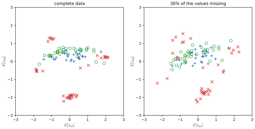
fig12_11. Download: PDF · SVGThe zero-noise limit: EM for PCA
As \(\sigma^2\to0\) PPCA becomes standard PCA, and EM still gives a valid algorithm (Roweis, 1998). By (12.55) only \(\E[\mathbf{z}_n]\) is needed, and \(\mathbf{M}=\mathbf{W}^\T\mathbf{W}\). Let \(\widetilde{\mathbf{X}}\) be the \(N\times D\) centred data matrix and \(\bm{\Omega}\) the \(M\times N\) matrix whose \(n\)th column is \(\E[\mathbf{z}_n]\) (erratum: the first printing says "\(D\times M\) whose \(n\)th row"). The E step (12.54) and the M step (12.56) become
\[ \bm{\Omega}=(\mathbf{W}_{\rm old}^\T\mathbf{W}_{\rm old})^{-1}\mathbf{W}_{\rm old}^\T\widetilde{\mathbf{X}}^\T , \tag{12.58} \] \[ \mathbf{W}_{\rm new}=\widetilde{\mathbf{X}}^\T\bm{\Omega}^\T(\bm{\Omega}\bm{\Omega}^\T)^{-1} \tag{12.59} \](erratum: the first printing has \(\widetilde{\mathbf{X}}\) instead of \(\widetilde{\mathbf{X}}^\T\) in (12.58)). The E step projects the data orthogonally onto the current subspace; the M step re-fits the subspace by least squares with the projections held fixed (Exercise 12.17). Both are on-line friendly.
Result 12.12 (EM for PCA is subspace iteration)
(a) As \(\sigma^2\to0\), the E step (12.54)–(12.55) and the M step (12.56) tend to (12.58)–(12.59). (b) Combining the two steps,
\[ \mathbf{W}_{\rm new}=\mathbf{S}\mathbf{W}_{\rm old}\big(\mathbf{W}_{\rm old}^\T\mathbf{S}\mathbf{W}_{\rm old}\big)^{-1}\mathbf{W}_{\rm old}^\T\mathbf{W}_{\rm old}, \]so the column space of \(\mathbf{W}\) is mapped to its image under \(\mathbf{S}\): after \(t\) iterations it is \(\mathbf{S}^t\) applied to the initial column space. If \(\lambda_M\gt\lambda_{M+1}\) and \(\mathbf{U}_M^\T\mathbf{W}_0\) is invertible, the column space converges to the principal subspace, with error decreasing like \((\lambda_{M+1}/\lambda_M)^t\). (c) The E step minimises the reconstruction cost \(\lVert\widetilde{\mathbf{X}}-\bm{\Omega}^\T\mathbf{W}^\T\rVert_F^2\) over \(\bm{\Omega}\) with \(\mathbf{W}\) fixed, and the M step minimises it over \(\mathbf{W}\) with \(\bm{\Omega}\) fixed, so the cost never increases.
Proof
(a) As \(\sigma^2\to0\), \(\mathbf{M}\)
(b) Substitute (12.58) into (12.59), using \(\widetilde{\mathbf{X}}^\T\widetilde{\mathbf{X}}\)
(c) \(\lVert\widetilde{\mathbf{X}}-\bm{\Omega}^\T\mathbf{W}^\T\rVert_F^2\)
Bishop's physical picture (\(D=2\), \(M=1\)): the subspace is a rod and each point is tied to it by a spring obeying Hooke's law, with energy proportional to the squared length. In the E step the rod is held fixed and the attachment points slide along it to minimise the energy, ending at the orthogonal projections. In the M step the attachment points are frozen and the rod is released to its minimum-energy position. Figure 12.12 shows the iterations.
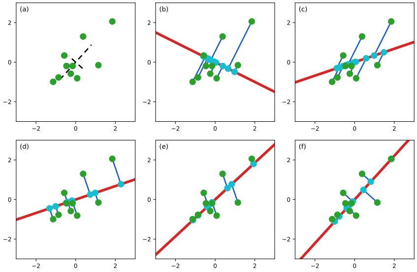
fig12_12. Download: PDF · SVG12.2.3 Bayesian PCA
So far \(M\) was given. For visualisation one takes \(M=2\), but in general the right value is unclear. One can look for a gap in the eigenvalue spectrum (Figure 12.4), but often there is none. Cross-validation on the likelihood is possible (PPCA has one) but costly, especially for a mixture of PPCA models where each component needs its own dimension (Tipping and Bishop, 1999a). A Bayesian approach would integrate out \(\bm{\mu}\), \(\mathbf{W}\) and \(\sigma^2\) and compare the marginal likelihoods of different \(M\); this is intractable but can be approximated variationally (Bishop, 1999b). The book presents a simpler method based on the evidence approximation (Bishop, 1999a), appropriate when \(N\) is large and the posterior is sharply peaked. It uses automatic relevance determination (ARD, Section 7.2.2): each column \(\mathbf{w}_i\) of \(\mathbf{W}\) gets its own Gaussian prior with precision \(\alpha_i\),
\[ p(\mathbf{W}\given\bm{\alpha})=\prod_{i=1}^M\Big(\frac{\alpha_i}{2\pi}\Big)^{D/2}\exp\Big\{-\frac12\alpha_i\mathbf{w}_i^\T\mathbf{w}_i\Big\}. \tag{12.60} \]The hyperparameters are chosen by maximising the marginal likelihood
\[ p(\mathbf{X}\given\bm{\alpha},\bm{\mu},\sigma^2)=\int p(\mathbf{X}\given\mathbf{W},\bm{\mu},\sigma^2)\,p(\mathbf{W}\given\bm{\alpha})\,\d\mathbf{W}, \tag{12.61} \]with \(\bm{\mu}\) and \(\sigma^2\) treated as parameters (no priors), and \(\ln p(\mathbf{X}\given\mathbf{W},\bm{\mu},\sigma^2)\) given by (12.43). Some \(\alpha_i\) go to infinity, forcing \(\mathbf{w}_i\to\mathbf{0}\) (its posterior collapses onto the origin): a sparse solution. The effective dimension of the principal subspace is the number of finite \(\alpha_i\), and the surviving columns are the "relevant" ones. The Bayesian criterion trades the improved fit from more columns against the complexity they add, as in the relevance vector machine (Section 7.2). The integral is intractable, and with a Laplace approximation and a sharply peaked posterior the re-estimation equation becomes
\[ \alpha_i^{\rm new}=\frac{D}{\mathbf{w}_i^\T\mathbf{w}_i} , \tag{12.62} \]the analogue of (3.98) with \(D\) parameters per column. These updates are interleaved with EM for \(\mathbf{W}\) and \(\sigma^2\): the E step is still (12.54)–(12.55), the \(\sigma^2\) update is still (12.57), and only the \(\mathbf{W}\) update changes, to
\[ \mathbf{W}_{\rm new}=\Big[\sum_{n=1}^N(\mathbf{x}_n-\bar{\mathbf{x}})\E[\mathbf{z}_n]^\T\Big]\Big[\sum_{n=1}^N\E[\mathbf{z}_n\mathbf{z}_n^\T]+\sigma^2\mathbf{A}\Big]^{-1},\qquad\mathbf{A}=\diag(\alpha_i). \tag{12.63} \]Filling the gap 12.6: the ARD re-estimation (12.62) and the M step (12.63) p. 583
The book says (12.62) "follows from (3.98)". Here is the Laplace-approximation argument that gives the general update \(\alpha_i\)
Derivation
Laplace approximation of (12.61). Let \(\mathbf{w}\)
Differentiating in \(\alpha_i\). \(\mathbf{W}^\star\) depends on \(\bm{\alpha}\), but because it is a stationary point of \(F\), that dependence does not contribute to the derivative of the first two terms. As in the evidence framework of Section 3.5, the dependence of \(\mathbf{H}_{\rm lik}\) on \(\bm{\alpha}\) through \(\mathbf{W}^\star\) is neglected, so \(\partial\mathbf{H}/\partial\alpha_i\) is the indicator of the block of column \(i\) and \(\partial\ln\lvert\mathbf{H}\rvert/\partial\alpha_i\)
As in (3.91)–(3.92), \(\gamma_i\in[0,D]\) counts how many of the \(D\) parameters of column \(i\) are determined by the data rather than by the prior (\(\bm{\Sigma}\preceq\mathbf{A}_D^{-1}\) gives \(\alpha_i\Tr\bm{\Sigma}_{ii}\le D\)). When the posterior is sharply peaked, \(\mathbf{H}_{\rm lik}\) grows like \(N\), \(\bm{\Sigma}_{ii}=O(1/N)\), and \(\gamma_i\to D\): this is (12.62), the counterpart of the large-data form (3.98). (Formally, (12.62) is also what one gets by maximising \(F\) jointly over \(\mathbf{W}\) and \(\bm{\alpha}\): \(\partial F/\partial\alpha_i\)
The M step (12.63). With the prior, EM maximises the expected complete-data log likelihood plus \(\ln p(\mathbf{W}\given\bm{\alpha})\)
and multiplying by \(\sigma^2\) and collecting the \(\mathbf{W}\) terms gives (12.63). The matrix \(\sum_n\E[\mathbf{z}_n\mathbf{z}_n^\T]+\sigma^2\mathbf{A}\) is positive definite, so this is the unique maximiser of a concave quadratic. The prior does not involve \(\sigma^2\), so the \(\sigma^2\) step is still (12.57). ∎
Algorithm 12.3 (Bayesian PCA by EM with ARD; Bishop, 1999a)
- Choose \(M\) generously (e.g. \(M=D-1\)); set \(\bm{\mu}=\bar{\mathbf{x}}\); initialise \(\mathbf{W}\), \(\sigma^2\) and \(\bm{\alpha}\) (e.g. all \(\alpha_i\) small).
- E step: \(\E[\mathbf{z}_n]\), \(\E[\mathbf{z}_n\mathbf{z}_n^\T]\) by (12.54)–(12.55).
- M step: \(\mathbf{W}\) by (12.63), then \(\sigma^2\) by (12.57).
- Hyperparameters: \(\alpha_i\)
\({}=D/\lVert\mathbf{w}_i\rVert^2\) (12.62). Repeat 2–4; columns whose \(\alpha_i\) diverge are pruned, and the number of surviving columns estimates the dimension of the principal subspace.
With \(M=D-1\) the model can represent everything from a full-covariance Gaussian (all \(\alpha_i\) finite) to an isotropic one (all \(\alpha_i\to\infty\)); a smaller \(M\) saves computation but caps the dimension that can be found. A caution about what the iteration optimises: substituting (12.62) into \(F\) of Gap 12.6 gives \(F\)
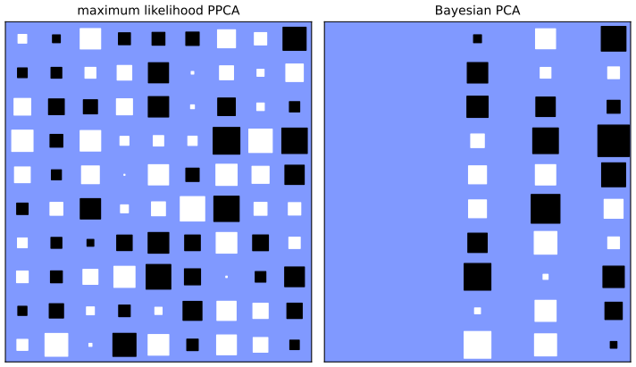
fig12_14. Download: PDF · SVGGibbs sampling for Bayesian PCA
Bayesian PCA also illustrates Gibbs sampling (Section 11.3). Figure 12.15 follows \(\ln\alpha_i\) for data in \(D=4\) dimensions with \(M=3\), generated from a PPCA model with one direction of high variance and low-variance noise elsewhere. The posterior has three modes: at any time one \(\alpha_i\) is small (its column carries the strong direction) and the other two are large (their columns are switched off), and the sampler jumps abruptly between the modes. The three modes are images of each other under permutation of the columns of \(\mathbf{W}\), which leaves the likelihood and the prior unchanged; this is the continuous-latent analogue of label switching in mixtures.
Algorithm 12.4 (a Gibbs sampler for Bayesian PCA)
Model: (12.31), (12.32) with \(\tau=\sigma^{-2}\), the ARD prior (12.60), and conjugate hyperpriors \(\alpha_i\sim\Gam(a_\alpha,b_\alpha)\), \(\tau\sim\Gam(a_\tau,b_\tau)\), \(\bm{\mu}\sim\N(\mathbf{0},\beta^{-1}\mathbf{I})\). Cycle through:
- \(\mathbf{z}_n\sim\N\big(\mathbf{M}^{-1}\mathbf{W}^\T(\mathbf{x}_n-\bm{\mu}),\,\tau^{-1}\mathbf{M}^{-1}\big)\) for each \(n\), the posterior (12.42).
- Each row \(\widetilde{\mathbf{w}}_d\) of \(\mathbf{W}\): \(\N\big(\tau\bm{\Sigma}_w\sum_n\mathbf{z}_n(x_{nd}-\mu_d),\,\bm{\Sigma}_w\big)\) with \(\bm{\Sigma}_w\)
\({}=\big(\mathbf{A}+\tau\sum_n\mathbf{z}_n\mathbf{z}_n^\T\big)^{-1}\). - \(\alpha_i\sim\Gam\big(a_\alpha+D/2,\;b_\alpha+\lVert\mathbf{w}_i\rVert^2/2\big)\) for each \(i\).
- \(\tau\sim\Gam\big(a_\tau+ND/2,\;b_\tau+Q/2\big)\), where \(Q\)
\({}=\sum_n\lVert\mathbf{x}_n-\mathbf{W}\mathbf{z}_n-\bm{\mu}\rVert^2\). - \(\bm{\mu}\sim\N\big(\mathbf{m}_\mu,(\beta+N\tau)^{-1}\mathbf{I}\big)\), where \(\mathbf{m}_\mu\)
\({}=\tau\sum_n(\mathbf{x}_n-\mathbf{W}\mathbf{z}_n)/(\beta+N\tau)\).
Derivation of the conditionals
Each conditional is proportional to the joint density
\[ \prod_n\N(\mathbf{x}_n\given\mathbf{W}\mathbf{z}_n+\bm{\mu},\tau^{-1}\mathbf{I})\,\N(\mathbf{z}_n\given\mathbf{0},\mathbf{I})\times p(\mathbf{W}\given\bm{\alpha})\prod_ip(\alpha_i)\,p(\tau)\,p(\bm{\mu}), \]viewed as a function of one block. (1) The \(\mathbf{z}_n\) are conditionally independent and each has the PPCA posterior (Result 12.6). (2) The prior (12.60) makes all entries \(W_{di}\) independent with variance \(\alpha_i^{-1}\), so each row has prior \(\N(\widetilde{\mathbf{w}}_d\given\mathbf{0},\mathbf{A}^{-1})\), and given \(\mathbf{Z}\) the likelihood factorises over rows: \(\prod_n\N(x_{nd}\given\widetilde{\mathbf{w}}_d^\T\mathbf{z}_n+\mu_d,\tau^{-1})\). Row \(d\) is therefore a Bayesian linear regression of \(x_{nd}-\mu_d\) on \(\mathbf{z}_n\), and completing the square gives the stated Gaussian (as in (3.53)–(3.54)). (3) As a function of \(\alpha_i\), \(\alpha_i^{D/2}e^{-\alpha_i\lVert\mathbf{w}_i\rVert^2/2}\times\alpha_i^{a_\alpha-1}e^{-b_\alpha\alpha_i}\) is a Gamma kernel (toolkit). (4) Likewise \(\tau^{ND/2}e^{-\tau Q/2}\tau^{a_\tau-1}e^{-b_\tau\tau}\) with \(Q\)
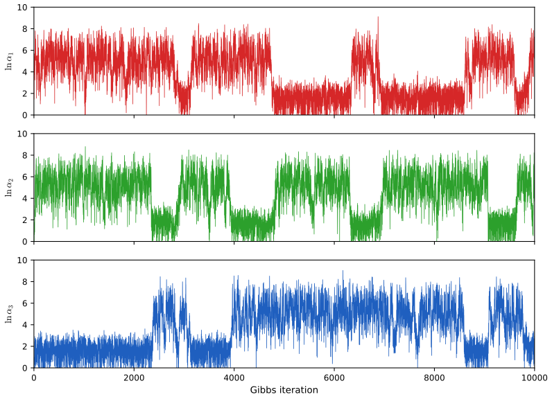
fig12_15. Download: PDF · SVGThe model here puts a prior on \(\mathbf{W}\) only; a fully Bayesian treatment with priors on \(\bm{\mu}\), \(\sigma^2\) and \(\bm{\alpha}\), fitted variationally, is given by Bishop (1999b), and Minka (2001c) discusses Bayesian choices of the dimension of PCA.
12.2.4 Factor analysis
Definition 12.3 (factor analysis)
Factor analysis is the linear-Gaussian latent variable model with \(p(\mathbf{z})\)
where \(\bm{\Psi}\) is a \(D\times D\) diagonal matrix with positive entries. The columns of \(\mathbf{W}\) are the factor loadings and the diagonal entries of \(\bm{\Psi}\) are the uniquenesses. By the linear-Gaussian result (2.115) (or the moment argument of (12.37)–(12.38)), \(p(\mathbf{x})\)
The only difference from PPCA is a diagonal instead of an isotropic noise covariance. As in PPCA, the observed variables are independent given \(\mathbf{z}\): the model explains the covariance between variables through \(\mathbf{W}\) and gives each variable its own independent noise variance in \(\bm{\Psi}\). Factor analysis is as old as PCA (Everitt, 1984; Bartholomew, 1987; Basilevsky, 1994). Lawley (1953) and Anderson (1963) showed that at the stationary points of the likelihood of a factor model with \(\bm{\Psi}=\sigma^2\mathbf{I}\) the columns of \(\mathbf{W}\) are scaled eigenvectors of \(\mathbf{S}\) and \(\sigma^2\) is the average discarded eigenvalue; Tipping and Bishop (1999b) showed that the maximum uses the principal eigenvectors (Result 12.8).
Factor analysis has the same rotational invariance as PPCA (Exercise 12.19): with \(\widetilde{\mathbf{W}}\)
The maximum likelihood estimate of \(\bm{\mu}\) is again \(\bar{\mathbf{x}}\) (Exercise 12.20; the argument of Result 12.7 applies verbatim because \(\mathbf{C}\)
which needs only \(M\times M\) inversions (and the trivial inverse of the diagonal \(\bm{\Psi}\)). The M step is
\[ \mathbf{W}_{\rm new}=\Big[\sum_{n=1}^N(\mathbf{x}_n-\bar{\mathbf{x}})\E[\mathbf{z}_n]^\T\Big]\Big[\sum_{n=1}^N\E[\mathbf{z}_n\mathbf{z}_n^\T]\Big]^{-1}, \tag{12.69} \] \[ \bm{\Psi}_{\rm new}=\diag\Big\{\mathbf{S}-\mathbf{W}_{\rm new}\frac1N\sum_{n=1}^N\E[\mathbf{z}_n](\mathbf{x}_n-\bar{\mathbf{x}})^\T\Big\}, \tag{12.70} \]where \(\diag\{\cdot\}\) sets the off-diagonal elements to zero.
Filling the gap 12.7: the EM algorithm for factor analysis pp. 585–586, (12.66)–(12.70); Exercises 12.21, 12.22
The book states the E and M steps. Here they are derived: the E step from the linear-Gaussian posterior, the M step from the expected complete-data log likelihood.
Derivation
E step. In the linear-Gaussian result (2.116) take prior precision \(\bm{\Lambda}=\mathbf{I}\), prior mean \(\mathbf{0}\), \(\mathbf{A}=\mathbf{W}\), \(\mathbf{b}\)
Expected complete-data log likelihood. Write \(\mathbf{y}_n\)
M step for \(\mathbf{W}\). Differentiating (toolkit), \(\partial\mathcal{Q}/\partial\mathbf{W}\)
M step for \(\bm{\Psi}\). With \(\bm{\Psi}\)
Keeping the diagonal and dividing by \(N\) gives (12.70). (The diagonals of \(\mathbf{W}\E[\mathbf{z}]\mathbf{y}^\T\) and of its transpose coincide, so it does not matter which cross term is cancelled.) As in PPCA, maximising over \(\mathbf{W}\) first and then over \(\bm{\Psi}\) at \(\mathbf{W}_{\rm new}\) gives the joint maximiser, because \(\mathbf{W}_{\rm new}\) does not depend on \(\bm{\Psi}\). (Erratum: in the first printing the left-hand sides of (12.69)–(12.70) are typeset incorrectly.) ∎
Algorithm 12.5 (EM for factor analysis; Rubin and Thayer, 1982)
- Set \(\bm{\mu}=\bar{\mathbf{x}}\); initialise \(\mathbf{W}\) (e.g. from PPCA) and \(\bm{\Psi}\) (e.g. \(\diag\mathbf{S}\)).
- E step: \(\mathbf{G}\) (12.68), \(\E[\mathbf{z}_n]\) (12.66), \(\E[\mathbf{z}_n\mathbf{z}_n^\T]\) (12.67).
- M step: \(\mathbf{W}\) (12.69), then \(\bm{\Psi}\) (12.70).
- Evaluate \(\ln p(\mathbf{X})\) with \(\mathbf{C}\)
\({}=\mathbf{W}\mathbf{W}^\T+\bm{\Psi}\) and repeat until it stops increasing.
A Bayesian factor analysis follows from the techniques of the book (for example ARD priors on the loadings, as in Section 12.2.3). The number of free parameters of the factor analysis covariance is \(DM+D-M(M-1)/2\) (Exercise 12.18): the single \(\sigma^2\) of PPCA is replaced by \(D\) uniquenesses, and the rotations are still redundant.
The two models differ in how they behave when the data are transformed (Exercise 12.25). Fitting PCA or PPCA to rotated data gives the same fit with \(\mathbf{W}\) rotated accordingly, but rescaling the variables (changing units) changes the principal directions. Factor analysis has the opposite property: a component-wise rescaling of the data is absorbed by rescaling the rows of \(\mathbf{W}\) and the entries of \(\bm{\Psi}\).
Result 12.13 (how the fits transform; Exercise 12.25)
Consider the general linear-Gaussian model \(p(\mathbf{z})\)
Proof
By the change-of-variables formula for a Gaussian, \(\N(\mathbf{A}\mathbf{x}\given\bm{\mu}',\mathbf{C}')\)
12.3 Kernel PCA
Chapter 6 showed that an algorithm that uses the data only through inner products \(\mathbf{x}^\T\mathbf{x}'\) can be made nonlinear by replacing them with a kernel \(k(\mathbf{x},\mathbf{x}')\). Applied to PCA this gives kernel PCA (Schölkopf, Smola and Müller, 1998). Assume for now that the data are centred, \(\sum_n\mathbf{x}_n=\mathbf{0}\). The principal components solve
\[ \mathbf{S}\mathbf{u}_i=\lambda_i\mathbf{u}_i , \tag{12.71} \] \[ \mathbf{S}=\frac1N\sum_{n=1}^N\mathbf{x}_n\mathbf{x}_n^\T , \tag{12.72} \]with \(\mathbf{u}_i^\T\mathbf{u}_i=1\). Now map each point into a feature space, \(\mathbf{x}_n\mapsto\bm{\phi}(\mathbf{x}_n)\), and do PCA there; linear projections in feature space become nonlinear functions of \(\mathbf{x}\) (Figure 12.16 of the book). Notation warning: in this section \(M\) is the dimension of the feature space (possibly infinite) and \(\mathbf{C}\) is the feature-space covariance, not the PPCA quantities of Section 12.2. Assuming for the moment that the features are centred too, \(\sum_n\bm{\phi}(\mathbf{x}_n)\)
that is,
\[ \frac1N\sum_{n=1}^N\bm{\phi}(\mathbf{x}_n)\big\{\bm{\phi}(\mathbf{x}_n)^\T\mathbf{v}_i\big\}=\lambda_i\mathbf{v}_i . \tag{12.75} \]If \(\lambda_i\gt0\), (12.75) expresses \(\mathbf{v}_i\) as a combination of the feature vectors,
\[ \mathbf{v}_i=\sum_{n=1}^Na_{in}\bm{\phi}(\mathbf{x}_n),\qquad a_{in}=\frac{\bm{\phi}(\mathbf{x}_n)^\T\mathbf{v}_i}{N\lambda_i} . \tag{12.76} \]Substituting back,
\[ \frac1N\sum_{n=1}^N\bm{\phi}(\mathbf{x}_n)\bm{\phi}(\mathbf{x}_n)^\T\sum_{m=1}^Na_{im}\bm{\phi}(\mathbf{x}_m)=\lambda_i\sum_{n=1}^Na_{in}\bm{\phi}(\mathbf{x}_n), \tag{12.77} \]and multiplying by \(\bm{\phi}(\mathbf{x}_l)^\T\) turns every feature vector into a kernel value \(k(\mathbf{x}_n,\mathbf{x}_m)\)
(erratum: the first printing has the upper limit \(m\) instead of \(N\) in the inner sum). With the Gram matrix \(\mathbf{K}\), \(K_{nm}\)
and it suffices to solve
\[ \mathbf{K}\mathbf{a}_i=\lambda_iN\mathbf{a}_i . \tag{12.80} \]The coefficients are normalised by requiring unit feature-space eigenvectors,
\[ 1=\mathbf{v}_i^\T\mathbf{v}_i=\sum_{n=1}^N\sum_{m=1}^Na_{in}a_{im}\bm{\phi}(\mathbf{x}_n)^\T\bm{\phi}(\mathbf{x}_m)=\mathbf{a}_i^\T\mathbf{K}\mathbf{a}_i=\lambda_iN\mathbf{a}_i^\T\mathbf{a}_i , \tag{12.81} \]and the projection of a point \(\mathbf{x}\) onto the \(i\)th component needs only kernel evaluations:
\[ y_i(\mathbf{x})=\bm{\phi}(\mathbf{x})^\T\mathbf{v}_i=\sum_{n=1}^Na_{in}\bm{\phi}(\mathbf{x})^\T\bm{\phi}(\mathbf{x}_n)=\sum_{n=1}^Na_{in}k(\mathbf{x},\mathbf{x}_n). \tag{12.82} \]Result 12.14 (kernel PCA through the Gram matrix; Exercise 12.26)
Let \(\bm{\Phi}\) be the \(N\times M\) matrix with rows \(\bm{\phi}(\mathbf{x}_n)^\T\), so \(\mathbf{K}=\bm{\Phi}\bm{\Phi}^\T\) and \(\mathbf{C}\)
Proof
(a) \(\mathbf{C}\mathbf{v}\)
(b) \(\lVert\mathbf{v}\rVert^2\)
(c) Any solution of (12.80) solves (12.79) (multiply by \(\mathbf{K}\)). Conversely, \(\mathbf{K}\) is symmetric, so \(\R^N\) is the orthogonal sum of its range and its null space; write \(\mathbf{a}\)
(d) The rank of \(\mathbf{C}\)
So far the features were assumed centred. In general they are not, and the mean \(\frac1N\sum_l\bm{\phi}(\mathbf{x}_l)\) cannot be subtracted explicitly when the feature space is not available. The centred features
\[ \widetilde{\bm{\phi}}(\mathbf{x}_n)=\bm{\phi}(\mathbf{x}_n)-\frac1N\sum_{l=1}^N\bm{\phi}(\mathbf{x}_l) \tag{12.83} \]have Gram matrix
\[ \begin{aligned}\widetilde{K}_{nm}&=\widetilde{\bm{\phi}}(\mathbf{x}_n)^\T\widetilde{\bm{\phi}}(\mathbf{x}_m)\\ &=\bm{\phi}(\mathbf{x}_n)^\T\bm{\phi}(\mathbf{x}_m)-\frac1N\sum_{l=1}^N\bm{\phi}(\mathbf{x}_n)^\T\bm{\phi}(\mathbf{x}_l)\\ &\qquad-\frac1N\sum_{l=1}^N\bm{\phi}(\mathbf{x}_l)^\T\bm{\phi}(\mathbf{x}_m)+\frac{1}{N^2}\sum_{j=1}^N\sum_{l=1}^N\bm{\phi}(\mathbf{x}_j)^\T\bm{\phi}(\mathbf{x}_l)\\ &=k(\mathbf{x}_n,\mathbf{x}_m)-\frac1N\sum_{l=1}^Nk(\mathbf{x}_l,\mathbf{x}_m)\\ &\qquad-\frac1N\sum_{l=1}^Nk(\mathbf{x}_n,\mathbf{x}_l)+\frac{1}{N^2}\sum_{j=1}^N\sum_{l=1}^Nk(\mathbf{x}_j,\mathbf{x}_l),\end{aligned} \tag{12.84} \]or in matrix form
\[ \widetilde{\mathbf{K}}=\mathbf{K}-\mathbf{1}_N\mathbf{K}-\mathbf{K}\mathbf{1}_N+\mathbf{1}_N\mathbf{K}\mathbf{1}_N , \tag{12.85} \]where \(\mathbf{1}_N\) is the \(N\times N\) matrix with every entry \(1/N\).
Result 12.15 (centring in feature space)
With the centring matrix \(\mathbf{H}=\mathbf{I}-\mathbf{1}_N\), \(\widetilde{\mathbf{K}}\)
\(\widetilde{\mathbf{K}}\mathbf{1}\)
Proof
In matrix form (12.83) is \(\widetilde{\bm{\Phi}}\)
With the linear kernel \(k(\mathbf{x},\mathbf{x}')\)
Algorithm 12.6 (kernel PCA)
- Compute \(K_{nm}\)
\({}=k(\mathbf{x}_n,\mathbf{x}_m)\) and centre it, \(\widetilde{\mathbf{K}}\) \({}=\mathbf{H}\mathbf{K}\mathbf{H}\) (12.85). - Find the leading eigenpairs \(\widetilde{\mathbf{K}}\widetilde{\mathbf{a}}_i\)
\({}=\kappa_i\widetilde{\mathbf{a}}_i\), \(\lVert\widetilde{\mathbf{a}}_i\rVert\) \({}=1\), \(\kappa_i\gt0\); the feature-space variances are \(\lambda_i=\kappa_i/N\). - Normalise \(\mathbf{a}_i\)
\({}=\widetilde{\mathbf{a}}_i/\sqrt{\kappa_i}\) (12.81). - Project: \(y_i(\mathbf{x})\)
\({}=\sum_na_{in}\widetilde{k}(\mathbf{x},\mathbf{x}_n)\) (Result 12.15); for training points \(y_i(\mathbf{x}_n)\) \({}=(\widetilde{\mathbf{K}}\mathbf{a}_i)_n\) \({}=\sqrt{\kappa_i}\,\widetilde{a}_{in}\).
Figure 12.17 applies kernel PCA with the "Gaussian" kernel
\[ k(\mathbf{x},\mathbf{x}')=\exp\big(-\lVert\mathbf{x}-\mathbf{x}'\rVert^2/0.1\big) \tag{12.86} \]to a synthetic two-dimensional data set, drawing contours along which the projection
\[ \bm{\phi}(\mathbf{x})^\T\mathbf{v}_i=\sum_{n=1}^Na_{in}k(\mathbf{x},\mathbf{x}_n) \tag{12.87} \]is constant (in practice with the centred kernel \(\widetilde{k}\) of Result 12.15).
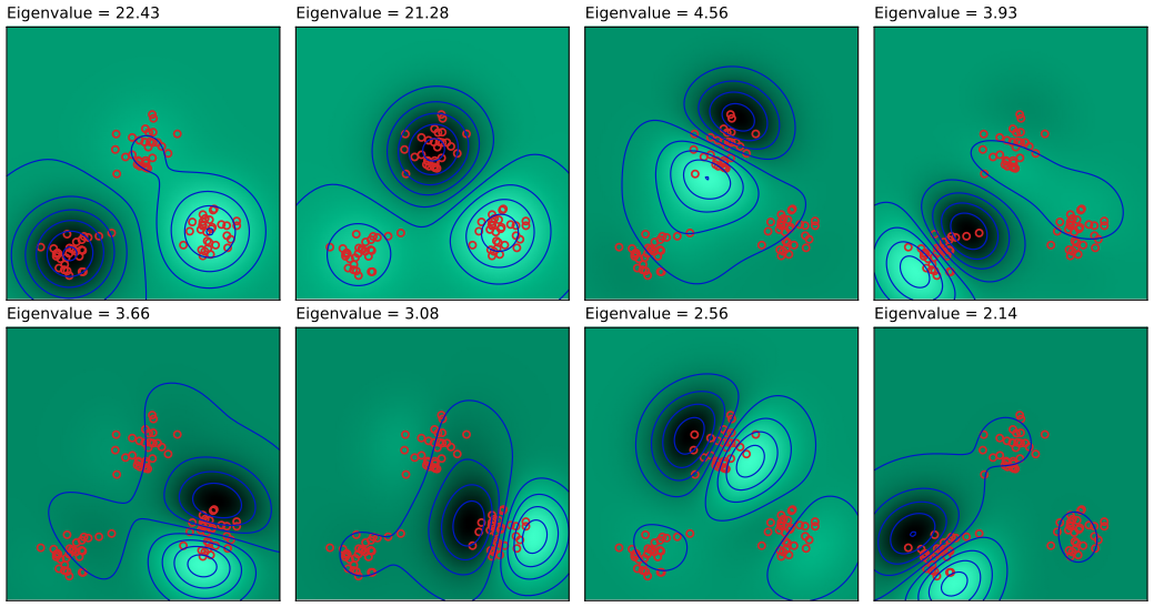
fig12_17. Download: PDF · SVGLimitations. Kernel PCA needs the eigenvectors of the \(N\times N\) matrix \(\widetilde{\mathbf{K}}\) rather than the \(D\times D\) matrix \(\mathbf{S}\), so for large data sets approximations are used. And while linear PCA can approximate a point by its projection onto the principal subspace,
\[ \widehat{\mathbf{x}}_n=\sum_{i=1}^L\big(\mathbf{x}_n^\T\mathbf{u}_i\big)\mathbf{u}_i , \tag{12.88} \]kernel PCA in general cannot: \(\bm{\phi}\) maps the \(D\)-dimensional data space onto a \(D\)-dimensional curved surface in feature space, and the projection of \(\bm{\phi}(\mathbf{x})\) onto the kernel principal subspace usually does not lie on that surface, so it has no pre-image \(\mathbf{x}\). Approximate pre-images can be computed (Bakir, Weston and Schölkopf, 2004).
12.4 Nonlinear Latent Variable Models
The linear-Gaussian models of this chapter are important, easy to analyse and fit, and useful as building blocks. This section sketches models that are nonlinear, non-Gaussian, or both. The two generalisations are related: any density can be obtained from a fixed simple density by a nonlinear change of variables (Exercise 12.28). In one dimension, if \(q\) and \(p\) are densities with distribution functions \(F_q\) and \(F_p\) and \(q\gt0\) everywhere, the increasing map \(y=f(x)=F_p^{-1}(F_q(x))\) turns \(x\sim q\) into \(y\sim p\), because it satisfies the differential equation
\[ p\big(f(x)\big)\,f'(x)=q(x), \]which is the change-of-variables formula (1.27) read backwards (see Exercise 12.28). Several practical latent variable models are built on this idea.
12.4.1 Independent component analysis
Keep the observed variables linear in the latent ones but let the latent distribution be non-Gaussian. Independent component analysis (ICA) takes a factorised latent distribution,
\[ p(\mathbf{z})=\prod_{j=1}^Mp(z_j). \tag{12.89} \]The motivating example is the "cocktail party": two people speak at once and two microphones record linear mixtures of the two voices (ignoring delays and echoes). If the constant mixing coefficients can be inferred from the recordings alone, the mixing can be inverted to recover each voice separately. This is blind source separation: neither the sources nor the mixing coefficients are observed (Cardoso, 1998). Following MacKay (2003), ignore the time ordering and treat the samples as i.i.d.; there are as many latent variables (voices) as observed ones (microphones), \(M=D\), and no noise term is needed, because a square nonsingular mixing does not produce a singular distribution.
Definition 12.4 (the noise-free square ICA model and its likelihood)
\(\mathbf{x}=\mathbf{A}\mathbf{z}\) with \(\mathbf{A}\) a nonsingular \(D\times D\) mixing matrix and independent sources \(z_j\sim p_j\). With the unmixing matrix \(\mathbf{B}=\mathbf{A}^{-1}\) (rows \(\mathbf{b}_j^\T\)), the change-of-variables formula gives \(p(\mathbf{x})\)
where \(g_j=(\ln p_j)'\) is applied componentwise. The likelihood is maximised by gradient methods.
Derivation of the gradient
\(\d\ln\lvert\det\mathbf{B}\rvert\)
The method needs non-Gaussian sources. In PPCA and factor analysis the latent distribution is a standard Gaussian, and the likelihood cannot distinguish \(\mathbf{W}\) from \(\mathbf{W}\mathbf{R}\) (12.39): the latent coordinates are determined only up to a rotation. A general Gaussian latent distribution does not help, because it is equivalent to the standard one (Exercise 12.4). Put differently, PCA rotates the data so that the coordinates are uncorrelated, and zero correlation is necessary for independence but not sufficient (Exercise 12.29). A common choice is the heavy-tailed density
\[ p(z_j)=\frac{1}{\pi\cosh(z_j)}=\frac{2}{\pi\big(e^{z_j}+e^{-z_j}\big)} \tag{12.90} \](erratum: the first printing has numerator 1 in the rightmost expression). It integrates to one (\(\int\operatorname{sech}z\,\d z=\pi\)), has variance \(\pi^2/4\) and heavier tails than a Gaussian (excess kurtosis 2), as many real signals do.
Result 12.16 (Gaussian sources cannot be unmixed)
If the sources are independent Gaussians (standardised to \(\mathbf{z}\sim\N(\mathbf{0},\mathbf{I})\)), then \(\mathbf{x}=\mathbf{A}\mathbf{z}\) and \(\mathbf{x}\)
Proof of the Gaussian part
\(\mathbf{x}=\mathbf{A}\mathbf{z}\) is Gaussian with mean \(\mathbf{0}\) and covariance \(\mathbf{A}\mathbf{A}^\T\) (an affine image of a Gaussian), and \((\mathbf{A}\mathbf{R})(\mathbf{A}\mathbf{R})^\T\)
The original ICA algorithm (Bell and Sejnowski, 1995) maximised an information-theoretic objective (infomax). A probabilistic formulation suggests generalisations, for example independent factor analysis (Attias, 1999a), with noisy observations, possibly different numbers of latent and observed variables, and source densities modelled by Gaussian mixtures, fitted by EM with a variational approximation for the posterior over the sources. The ICA literature is large (Jutten and Hérault, 1991; Comon et al., 1991; Amari et al., 1996; Hyvärinen and Oja, 1997, 2000; Stone, 2004, and others listed in the book).
12.4.2 Autoassociative neural networks
Neural networks (Chapter 5) can also reduce dimension without supervision. An autoassociative network has \(D\) inputs, \(D\) outputs and \(M\lt D\) hidden units (Figure 12.18 of the book), and is trained to reproduce its input, by minimising
\[ E(\mathbf{w})=\frac12\sum_{n=1}^N\lVert\mathbf{y}(\mathbf{x}_n,\mathbf{w})-\mathbf{x}_n\rVert^2 . \tag{12.91} \]Because \(M\lt D\), perfect reconstruction is impossible in general. The book states that with linear hidden units the error has a unique global minimum at which the network projects onto the principal subspace (Bourlard and Kamp, 1988; Baldi and Hornik, 1989), and that nonlinear hidden units do not help. Both claims follow from Section 12.1.2.
Result 12.17 (a network with linear outputs cannot beat PCA)
Let the hidden activations be \(\mathbf{h}\)
With linear hidden units the bound is attained, exactly when \(\mathbf{y}(\mathbf{x})\)
Proof
Whatever \(\mathbf{g}\) is, every output lies in the set \(\mathcal{A}\)
So two-layer networks bring nothing over standard PCA, which (via the singular value decomposition) is guaranteed to give the correct answer in finite time, with ordered eigenvalues and orthonormal eigenvectors. The situation changes with more layers (Figures 12.19 and 12.20 of the book): a network with a nonlinear first hidden layer, an \(M\)-unit second hidden layer (linear, say), a nonlinear third hidden layer and linear outputs computes two successive mappings, \(F_1:\R^D\to\R^M\) (a general nonlinear projection onto a subspace \(\mathcal{S}\)) and \(F_2:\R^M\to\R^D\) (a general embedding of \(\mathcal{S}\) back into the data space, which may be curved). Such a network performs nonlinear PCA and includes linear PCA as a special case, but the error (12.91) is no longer quadratic in the weights: training is a nonlinear optimisation with possible local minima, and \(M\) must be chosen in advance.
12.4.3 Modelling nonlinear manifolds
Many natural data lie near low-dimensional, noisy, curved manifolds, and capturing this explicitly can give better density models than general-purpose methods. The book surveys several approaches.
Mixtures of linear models
A curved manifold can be approximated piecewise linearly: cluster the data (for example with K-means) and apply PCA within each cluster. It is better to assign points by reconstruction error, so that one cost is optimised throughout (Kambhatla and Leen, 1997; Hinton, Dayan and Revow, 1997), but these methods still lack an overall density model. With PPCA one obtains a fully probabilistic mixture of probabilistic PCA models (Tipping and Bishop, 1999a),
\[ p(\mathbf{x})=\sum_{k=1}^K\pi_k\,\N\big(\mathbf{x}\given\bm{\mu}_k,\mathbf{W}_k\mathbf{W}_k^\T+\sigma_k^2\mathbf{I}\big), \]which has a discrete latent variable (the component) and a continuous one (the position within the component's subspace), and is fitted by EM.
Algorithm 12.7 (EM for a mixture of probabilistic PCA models)
- E step: responsibilities \(R_{nk}\propto\pi_k\N(\mathbf{x}_n\given\bm{\mu}_k,\mathbf{C}_k)\), normalised so that \(\sum_kR_{nk}=1\), with \(\mathbf{C}_k\)
\({}=\mathbf{W}_k\mathbf{W}_k^\T+\sigma_k^2\mathbf{I}\) (evaluated cheaply with Result 12.6). - M step: \(N_k=\sum_nR_{nk}\), \(\pi_k=N_k/N\), \(\bm{\mu}_k\)
\({}=\sum_nR_{nk}\mathbf{x}_n/N_k\), \(\mathbf{S}_k\) \({}=\sum_nR_{nk}(\mathbf{x}_n-\bm{\mu}_k)(\mathbf{x}_n-\bm{\mu}_k)^\T/N_k\); then \(\mathbf{W}_k\), \(\sigma_k^2\) from (12.45)–(12.46) applied to the eigendecomposition of \(\mathbf{S}_k\). - Repeat until the log likelihood stops increasing.
Why the M step is "PPCA on the weighted covariance"
With only the component label treated as latent (the continuous \(\mathbf{z}\) integrated out analytically), the expected complete-data log likelihood is \(\sum_n\sum_kR_{nk}\{\ln\pi_k+\ln\N(\mathbf{x}_n\given\bm{\mu}_k,\mathbf{C}_k)\}\). The \(\pi_k\) update is that of the Gaussian mixture (9.22). For component \(k\), the gradient in \(\bm{\mu}_k\) is \(\mathbf{C}_k^{-1}\sum_nR_{nk}(\mathbf{x}_n-\bm{\mu}_k)\), zero at the weighted mean whatever \(\mathbf{C}_k\) is. Substituting it, the trace trick gives
\[ \sum_nR_{nk}\ln\N(\mathbf{x}_n\given\bm{\mu}_k,\mathbf{C}_k)=-\frac{N_k}{2}\Big\{D\ln(2\pi)+\ln\lvert\mathbf{C}_k\rvert+\Tr\big(\mathbf{C}_k^{-1}\mathbf{S}_k\big)\Big\}, \]which is (12.44) with \(N_k\) and \(\mathbf{S}_k\) in place of \(N\) and \(\mathbf{S}\). Result 12.8 therefore gives its exact maximiser. (Tipping and Bishop, 1999a, also describe a variant that keeps \(\mathbf{z}\) as a latent variable and avoids the eigendecomposition.) ∎
A variational Bayesian treatment infers both the number of components and their dimensions (Bishop and Winn, 2000). Parameters such as \(\mathbf{W}\) or the noise variances can be tied across components, and replacing isotropic by diagonal noise gives a mixture of factor analysers (Ghahramani and Hinton, 1996a; Ghahramani and Beal, 2000). A hierarchical mixture of PPCA models supports interactive visualisation (Bishop and Tipping, 1998). The graphical models are drawn in Exercise 12.23.
Principal curves
Instead of many linear pieces, one can fit a single nonlinear model. PCA finds a linear subspace close to the data in least squares; principal curves (Hastie and Stuetzle, 1989) extend this to one-dimensional curves. A curve is a vector function \(\mathbf{f}(\lambda)\) of a scalar \(\lambda\), naturally parametrised by arc length. For a point \(\widehat{\mathbf{x}}\) let \(\lambda\)
A density can have many principal curves, and with finite data one restricts attention to smooth curves. Hastie and Stuetzle alternate, in a way reminiscent of EM for PCA, a projection step (each point gets the \(\lambda\) of its closest point on the curve) and a re-estimation step (each point of the curve becomes a weighted average of the data points that project nearby, the nearest ones weighted most), starting from the first principal component. If the curve is constrained to be a straight line, the procedure converges to the first principal component and is the power method: with \(\mathbf{f}(\lambda)\)
Multidimensional scaling, LLE and Isomap
Multidimensional scaling (MDS; Torgerson, 1952; Cox and Cox, 2000) seeks a low-dimensional configuration of points whose pairwise distances match given distances as closely as possible; with Euclidean distances the classical version is equivalent to PCA. Using general dissimilarities gives nonmetric MDS.
Result 12.18 (classical MDS is PCA)
Let \(\Delta_{nm}\)
Proof
Distances do not change under translation, so with \(\widetilde{\mathbf{x}}_n\)
Locally linear embedding (LLE; Roweis and Saul, 2000) first finds, for each point, the weights that best reconstruct it from its \(K\) nearest neighbours, \(\min\lVert\mathbf{x}_n-\sum_mW_{nm}\mathbf{x}_m\rVert^2\) subject to \(\sum_mW_{nm}=1\) (with \(W_{nm}=0\) for non-neighbours). Because the weights sum to one, the residual equals \(\lVert\sum_mW_{nm}(\mathbf{x}_n-\mathbf{x}_m)\rVert^2\)
Isomap (Tenenbaum, de Silva and Langford, 2000) applies classical MDS to geodesic distances measured along the manifold (for two points on a circle, the arc length rather than the chord). It (i) links each point to its \(K\) nearest neighbours, or to all points within a radius \(\epsilon\), with edges weighted by Euclidean distance; (ii) approximates geodesic distances by shortest paths in this graph (Dijkstra's or Floyd's algorithm); (iii) runs classical MDS (Result 12.18) on the matrix of graph distances.
Latent trait models and density networks
With continuous latent variables and discrete observed variables one obtains latent trait models (Bartholomew, 1987); for binary data, for example, \(p(x_d=1\given\mathbf{z})\)
A density network (MacKay, 1995; MacKay and Gibbs, 1999) takes \(\mathbf{z}\sim\N(\mathbf{0},\mathbf{I})\) and maps it through a multilayer neural network (Chapter 5), which with enough hidden units can approximate any nonlinear map, so very general densities result. The price is that the marginal likelihood is intractable. It is approximated by Monte Carlo (Chapter 11), \(p(\mathbf{x})\)
The generative topographic mapping
Restricting the nonlinear map and choosing a convenient latent distribution gives a model that is both nonlinear and cheap to train: the generative topographic mapping (GTM; Bishop, Svensén and Williams, 1996, 1997a, 1998b).
Definition 12.5 (GTM)
The latent distribution is a uniform distribution over a regular grid of \(K\) points \(\mathbf{z}_1,\dots,\mathbf{z}_K\) in a (usually two-dimensional) latent space, \(p(\mathbf{z})\)
This is a constrained Gaussian mixture: all components share one isotropic variance, and their centres lie on a smooth two-dimensional manifold, the image of the latent space under \(\mathbf{y}\).
Integrating over the latent space is a sum over the grid, and because \(\mathbf{y}\) is linear in \(\mathbf{W}\), the likelihood is available in closed form and can be maximised by EM. The curse of dimensionality that limits basis-function regression (Section 1.4) does not bite, because the basis functions live on the two-dimensional latent space whatever the dimension of the data.
Algorithm 12.8 (EM for GTM; Bishop, Svensén and Williams, 1998)
Let \(\bm{\Phi}\) be the \(K\times L\) matrix with entries \(\phi_l(\mathbf{z}_k)\), \(\mathbf{X}\) the \(N\times D\) data matrix.
- E step: responsibilities \(R_{kn}\)
\({}=\dfrac{\exp\{-\frac\beta2\lVert\mathbf{x}_n-\mathbf{W}\bm{\phi}(\mathbf{z}_k)\rVert^2\}}{\sum_{j}\exp\{-\frac\beta2\lVert\mathbf{x}_n-\mathbf{W}\bm{\phi}(\mathbf{z}_j)\rVert^2\}}\) (a \(K\times N\) matrix \(\mathbf{R}\)); \(\mathbf{G}\) \({}=\diag\big(\sum_nR_{kn}\big)\). - M step: solve \(\bm{\Phi}^\T\mathbf{G}\bm{\Phi}\,\mathbf{W}_{\rm new}^\T\)
\({}=\bm{\Phi}^\T\mathbf{R}\mathbf{X}\) (add \(\frac{\lambda}{\beta}\mathbf{I}\) to the matrix on the left for a Gaussian prior on \(\mathbf{W}\) with precision \(\lambda\)), then \(\dfrac{1}{\beta_{\rm new}}\) \({}=\dfrac{1}{ND}\sum_{n}\sum_kR_{kn}\lVert\mathbf{W}_{\rm new}\bm{\phi}(\mathbf{z}_k)-\mathbf{x}_n\rVert^2\). - Repeat. To visualise, plot each point at its posterior mean \(\sum_kR_{kn}\mathbf{z}_k\) in latent space (or at the posterior mode).
Derivation of the M step
The E step is Bayes' theorem for a mixture with equal weights \(1/K\) and a common covariance, so the normalising constants cancel. The expected complete-data log likelihood is
\[ \mathcal{Q}(\mathbf{W},\beta)=\sum_{n=1}^N\sum_{k=1}^KR_{kn}\Big\{\frac D2\ln\beta-\frac\beta2\lVert\mathbf{x}_n-\mathbf{W}\bm{\phi}_k\rVert^2\Big\}+\const,\qquad\bm{\phi}_k=\bm{\phi}(\mathbf{z}_k). \]Its gradient in \(\mathbf{W}\) is \(\beta\sum_n\sum_kR_{kn}(\mathbf{x}_n-\mathbf{W}\bm{\phi}_k)\bm{\phi}_k^\T\). Setting it to zero, \(\mathbf{W}\sum_kG_{kk}\bm{\phi}_k\bm{\phi}_k^\T\)
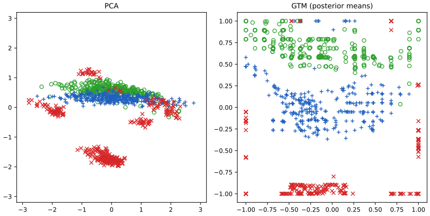
fig12_21. Download: PDF · SVGGTM and the self-organising map. GTM can be seen as a probabilistic version of the self-organising map (SOM; Kohonen, 1982, 1995), which also represents a two-dimensional manifold by a grid of prototype vectors \(\mathbf{m}_k\). The SOM resembles K-means: each data point is assigned to its nearest prototype \(c\)
Exercises
All 29 exercises of Chapter 12 (Bishop, pp. 599–603), with full solutions (hidden). Exercises marked www have official solutions (Svensén and Bishop); the solutions below are self-contained and were checked independently, and two slips in the published solution manuals are pointed out where they occur. Where the main text already contains the complete derivation, the solution summarises it and links to it. Difficulty stars are the book's.
Exercise 12.1 (★★, www). Prove by induction that the \(M\)-dimensional projection with maximal variance is given by the eigenvectors of the \(M\) largest eigenvalues of \(\mathbf{S}\): assuming the result for \(M\), maximise the variance along a new unit direction \(\mathbf{u}_{M+1}\) orthogonal to \(\mathbf{u}_1,\dots,\mathbf{u}_M\), using Lagrange multipliers for all the constraints.
Solution
The case \(M=1\) is Result 12.1. Assume \(\mathbf{u}_1,\dots,\mathbf{u}_M\) are the eigenvectors of the \(M\) largest eigenvalues. Maximise \(\mathbf{u}^\T\mathbf{S}\mathbf{u}\) subject to \(\mathbf{u}^\T\mathbf{u}=1\) and \(\mathbf{u}^\T\mathbf{u}_j=0\) (\(j\le M\)) with the Lagrangian \(\mathbf{u}^\T\mathbf{S}\mathbf{u}+\lambda(1-\mathbf{u}^\T\mathbf{u})+\sum_{j\le M}\eta_j\mathbf{u}^\T\mathbf{u}_j\). Stationarity: \(2\mathbf{S}\mathbf{u}-2\lambda\mathbf{u}+\sum_j\eta_j\mathbf{u}_j\)
\({}=\mathbf{0}\). Left-multiplying by \(\mathbf{u}_m^\T\) and using \(\mathbf{u}_m^\T\mathbf{S}\mathbf{u}\) \({}=\lambda_m\mathbf{u}_m^\T\mathbf{u}\) \({}=0\), \(\mathbf{u}_m^\T\mathbf{u}=0\), \(\mathbf{u}_m^\T\mathbf{u}_j\) \({}=\delta_{mj}\) gives \(\eta_m=0\). Hence \(\mathbf{S}\mathbf{u}\) \({}=\lambda\mathbf{u}\), the variance along \(\mathbf{u}\) is \(\mathbf{u}^\T\mathbf{S}\mathbf{u}\) \({}=\lambda\), and \(\mathbf{u}\) must be an eigenvector orthogonal to the first \(M\), so \(\lambda\in\{\lambda_{M+1},\dots,\lambda_D\}\); the maximum is \(\lambda_{M+1}\) at \(\mathbf{u}_{M+1}\). The total variance of the \((M+1)\)-dimensional projection is then \(\lambda_1+\dots+\lambda_{M+1}\), and Result 12.2(b) shows that no \((M+1)\)-dimensional projection does better, so the greedy construction is also globally optimal. Details: Result 12.2. Exercise 12.2 (★★). Show that the minimum of the distortion (12.15) subject to (12.7) is obtained when the \(\mathbf{u}_i\) are eigenvectors of \(\mathbf{S}\), using the matrix of multipliers \(\mathbf{H}\) in (12.93); show that \(\mathbf{H}\) may be taken symmetric and that the general solution of \(\mathbf{S}\widehat{\mathbf{U}}\)
\({}=\widehat{\mathbf{U}}\mathbf{H}\) gives the same \(J\) as the eigenvector solution. Solution
Only the symmetric part of \(\mathbf{H}\) enters (12.93), because \(\mathbf{I}-\widehat{\mathbf{U}}^\T\widehat{\mathbf{U}}\) is symmetric. Differentiating, \(2\mathbf{S}\widehat{\mathbf{U}}-2\widehat{\mathbf{U}}\mathbf{H}\)
\({}=\mathbf{0}\). With \(\mathbf{H}\) \({}=\bm{\Psi}\widehat{\bm{\Lambda}}\bm{\Psi}^\T\), the columns of \(\widehat{\mathbf{U}}\bm{\Psi}\) are orthonormal eigenvectors of \(\mathbf{S}\), so \(\widehat{\mathbf{U}}\) is any orthonormal basis of a span of \(D-M\) eigenvectors, and \(J\) \({}=\Tr(\widehat{\mathbf{U}}^\T\mathbf{S}\widehat{\mathbf{U}})\) \({}=\Tr\mathbf{H}\) \({}=\Tr\widehat{\bm{\Lambda}}\), the same value as for the eigenvector solution \(\widehat{\mathbf{U}}\bm{\Psi}\). The minimum (which exists and satisfies the multiplier rule) is the sum of the \(D-M\) smallest eigenvalues. Full details: Result 12.3. Exercise 12.3 (★). Verify that the vectors (12.30) have unit length when the \(\mathbf{v}_i\) do.
Solution
\(\lVert\mathbf{X}^\T\mathbf{v}_i\rVert^2\)
\({}=\mathbf{v}_i^\T\mathbf{X}\mathbf{X}^\T\mathbf{v}_i\) \({}=\mathbf{v}_i^\T(N\lambda_i\mathbf{v}_i)\) \({}=N\lambda_i\) by (12.28), so \(\lVert\mathbf{u}_i\rVert^2\) \({}=N\lambda_i/(N\lambda_i)\) \({}=1\). The same computation with \(\mathbf{v}_i^\T\mathbf{X}\mathbf{X}^\T\mathbf{v}_j\) \({}=N\lambda_j\mathbf{v}_i^\T\mathbf{v}_j\) shows that the \(\mathbf{u}_i\) are mutually orthogonal (Result 12.5). Exercise 12.4 (★, www). Replace the prior (12.31) by \(\N(\mathbf{z}\given\mathbf{m},\bm{\Sigma})\). Show that, after redefining the parameters, the marginal \(p(\mathbf{x})\) is the same as for the standard model, for any \(\mathbf{m}\) and \(\bm{\Sigma}\).
Solution
With \(\mathbf{x}\)
\({}=\mathbf{W}\mathbf{z}+\bm{\mu}+\bm{\epsilon}\) and \(\mathbf{z}\sim\N(\mathbf{m},\bm{\Sigma})\) independent of \(\bm{\epsilon}\), \(\mathbf{x}\) is Gaussian with mean \(\mathbf{W}\mathbf{m}+\bm{\mu}\) and covariance \(\mathbf{W}\bm{\Sigma}\mathbf{W}^\T+\sigma^2\mathbf{I}\). Factor \(\bm{\Sigma}\) \({}=\mathbf{L}\mathbf{L}^\T\) (Cholesky or symmetric square root) and set \(\widetilde{\mathbf{W}}\) \({}=\mathbf{W}\mathbf{L}\), \(\widetilde{\bm{\mu}}\) \({}=\bm{\mu}+\mathbf{W}\mathbf{m}\). Then \(p(\mathbf{x})\) \({}=\N(\mathbf{x}\given\widetilde{\bm{\mu}},\widetilde{\mathbf{W}}\widetilde{\mathbf{W}}^\T+\sigma^2\mathbf{I})\), the marginal of the standard model with parameters \(\widetilde{\mathbf{W}},\widetilde{\bm{\mu}},\sigma^2\). Equivalently, \(\mathbf{z}\) \({}=\mathbf{m}+\mathbf{L}\mathbf{z}'\) with \(\mathbf{z}'\sim\N(\mathbf{0},\mathbf{I})\) and \(\mathbf{W}\mathbf{z}+\bm{\mu}\) \({}=\widetilde{\mathbf{W}}\mathbf{z}'+\widetilde{\bm{\mu}}\). Conversely, the standard model is the case \(\mathbf{m}=\mathbf{0}\), \(\bm{\Sigma}=\mathbf{I}\), so the two families of distributions coincide and the extra parameters are redundant. (The solution manuals write the covariance as \(\sigma^2\mathbf{I}+\mathbf{W}^\T\bm{\Sigma}^{-1}\mathbf{W}\) or \(\mathbf{W}\bm{\Sigma}^{-1}\mathbf{W}^\T\); the correct form is \(\mathbf{W}\bm{\Sigma}\mathbf{W}^\T\).) Exercise 12.5 (★★). If \(\mathbf{x}\sim\N(\bm{\mu},\bm{\Sigma})\) in \(\R^D\) and \(\mathbf{y}\)
\({}=\mathbf{A}\mathbf{x}+\mathbf{b}\) with \(\mathbf{A}\) an \(M\times D\) matrix, show that \(\mathbf{y}\) is Gaussian, find its mean and covariance, and discuss \(M\lt D\), \(M=D\) and \(M\gt D\). Solution
The moment generating function is \(\E[e^{\mathbf{t}^\T\mathbf{y}}]\)
\({}=e^{\mathbf{t}^\T\mathbf{b}}\E[e^{(\mathbf{A}^\T\mathbf{t})^\T\mathbf{x}}]\) \({}=\exp\{\mathbf{t}^\T(\mathbf{A}\bm{\mu}+\mathbf{b})+\tfrac12\mathbf{t}^\T\mathbf{A}\bm{\Sigma}\mathbf{A}^\T\mathbf{t}\}\), using the Gaussian MGF \(\E[e^{\mathbf{s}^\T\mathbf{x}}]\) \({}=\exp(\mathbf{s}^\T\bm{\mu}+\tfrac12\mathbf{s}^\T\bm{\Sigma}\mathbf{s})\). This is the MGF of \(\N(\mathbf{A}\bm{\mu}+\mathbf{b},\mathbf{A}\bm{\Sigma}\mathbf{A}^\T)\), and the MGF determines the distribution. Assume \(\bm{\Sigma}\) positive definite. \(M\lt D\): \(\mathbf{A}\bm{\Sigma}\mathbf{A}^\T\) is positive definite iff \(\mathbf{A}\) has full row rank \(M\) (then \(\mathbf{v}^\T\mathbf{A}\bm{\Sigma}\mathbf{A}^\T\mathbf{v}\) \({}=0\) forces \(\mathbf{A}^\T\mathbf{v}=\mathbf{0}\), i.e. \(\mathbf{v}=\mathbf{0}\)), and \(\mathbf{y}\) has a proper density on \(\R^M\) (marginals of Gaussians are the special case where \(\mathbf{A}\) selects coordinates). \(M=D\): if \(\mathbf{A}\) is invertible, \(p(\mathbf{y})\) \({}=p_{\mathbf{x}}(\mathbf{A}^{-1}(\mathbf{y}-\mathbf{b}))/\lvert\det\mathbf{A}\rvert\), a nondegenerate Gaussian. \(M\gt D\): \(\operatorname{rank}(\mathbf{A}\bm{\Sigma}\mathbf{A}^\T)\) \({}\le D\) \({}\lt M\), so the covariance is singular: \(\mathbf{y}\) lives on the affine subspace \(\mathbf{b}+\operatorname{col}\mathbf{A}\) of dimension at most \(D\) and has no density on \(\R^M\). This is PPCA with \(\sigma^2=0\) (the map \(\mathbf{z}\mapsto\mathbf{W}\mathbf{z}+\bm{\mu}\) from \(\R^M\) to \(\R^D\), \(D\gt M\)), and it is why the noise term is needed for a proper density. Exercise 12.6 (★, www). Draw the directed graph of PPCA with the components of \(\mathbf{x}\) as separate nodes and verify that it has the independence structure of the naive Bayes model (Section 8.2.2).
Solution
Because \(\sigma^2\mathbf{I}\) is diagonal, \(p(\mathbf{x}\given\mathbf{z})\)
\({}=\prod_d\N(x_d\given\widetilde{\mathbf{w}}_d^\T\mathbf{z}+\mu_d,\sigma^2)\): each \(x_d\) has the single parent \(\mathbf{z}\) (the parameters \(\widetilde{\mathbf{w}}_d,\mu_d,\sigma^2\) are omitted) and there are no edges between the \(x_d\). This is the naive Bayes graph of Figure 8.24, with the class variable replaced by the continuous \(\mathbf{z}\). Every path between \(x_i\) and \(x_j\) passes tail-to-tail through \(\mathbf{z}\), so by d-separation \(x_i\perp\!\!\!\perp x_j\given\mathbf{z}\), exactly the naive Bayes assumption. Marginally the \(x_d\) are dependent (the path is open when \(\mathbf{z}\) is unobserved), which is how the model represents correlations: \(\cov[x_i,x_j]\) \({}=\widetilde{\mathbf{w}}_i^\T\widetilde{\mathbf{w}}_j\) for \(i\ne j\). Exercise 12.7 (★★). Using the results (2.270)–(2.271) for the mean and covariance of a general distribution, derive the marginal (12.35).
Solution
(2.270)–(2.271) are the laws of total expectation and total covariance: \(\E[\mathbf{x}]\)
\({}=\E_{\mathbf{z}}[\E[\mathbf{x}\given\mathbf{z}]]\) and \(\cov[\mathbf{x}]\) \({}=\E_{\mathbf{z}}[\cov[\mathbf{x}\given\mathbf{z}]]+\cov_{\mathbf{z}}[\E[\mathbf{x}\given\mathbf{z}]]\). (The second follows by writing \(\mathbf{x}-\E\mathbf{x}\) \({}=(\mathbf{x}-\E[\mathbf{x}\given\mathbf{z}])+(\E[\mathbf{x}\given\mathbf{z}]-\E\mathbf{x})\); the cross term has zero expectation because the first bracket has zero conditional mean.) Here \(\E[\mathbf{x}\given\mathbf{z}]\) \({}=\mathbf{W}\mathbf{z}+\bm{\mu}\) and \(\cov[\mathbf{x}\given\mathbf{z}]\) \({}=\sigma^2\mathbf{I}\), so \(\E[\mathbf{x}]\) \({}=\mathbf{W}\E[\mathbf{z}]+\bm{\mu}\) \({}=\bm{\mu}\) and \(\cov[\mathbf{x}]\) \({}=\sigma^2\mathbf{I}+\mathbf{W}\cov[\mathbf{z}]\mathbf{W}^\T\) \({}=\sigma^2\mathbf{I}+\mathbf{W}\mathbf{W}^\T\), which are (12.37)–(12.38). The distribution is Gaussian because \(\mathbf{x}\) is an affine function of the Gaussian vector \((\mathbf{z},\bm{\epsilon})\) (Exercise 12.5), or by the linear-Gaussian marginal (2.115); a direct computation is in Result 12.6. Exercise 12.8 (★★, www). Using (2.116), show that the posterior \(p(\mathbf{z}\given\mathbf{x})\) is (12.42).
Solution
Match \(p(\mathbf{z})\)
\({}=\N(\mathbf{z}\given\mathbf{0},\mathbf{I})\) with \(\N(\mathbf{z}\given\mathbf{m},\bm{\Lambda}^{-1})\) (so \(\mathbf{m}=\mathbf{0}\), \(\bm{\Lambda}=\mathbf{I}\)) and \(p(\mathbf{x}\given\mathbf{z})\) with \(\N(\mathbf{x}\given\mathbf{A}\mathbf{z}+\mathbf{b},\mathbf{L}^{-1})\) (so \(\mathbf{A}=\mathbf{W}\), \(\mathbf{b}=\bm{\mu}\), \(\mathbf{L}=\sigma^{-2}\mathbf{I}\)). By (2.116)–(2.117) the posterior covariance is \((\bm{\Lambda}+\mathbf{A}^\T\mathbf{L}\mathbf{A})^{-1}\) \({}=(\mathbf{I}+\sigma^{-2}\mathbf{W}^\T\mathbf{W})^{-1}\) \({}=\sigma^2(\sigma^2\mathbf{I}+\mathbf{W}^\T\mathbf{W})^{-1}\) \({}=\sigma^2\mathbf{M}^{-1}\), and the mean is \(\sigma^2\mathbf{M}^{-1}\{\mathbf{W}^\T\sigma^{-2}(\mathbf{x}-\bm{\mu})+\mathbf{0}\}\) \({}=\mathbf{M}^{-1}\mathbf{W}^\T(\mathbf{x}-\bm{\mu})\). This is (12.42); the first printing of the book has the covariance wrong (see the erratum noted at (12.42)). A self-contained derivation is in Result 12.6. Exercise 12.9 (★). Show that maximising (12.43) over \(\bm{\mu}\) gives \(\bm{\mu}_{\rm ML}=\bar{\mathbf{x}}\).
Solution
\(\partial/\partial\bm{\mu}\) of (12.43) is \(\mathbf{C}^{-1}\sum_n(\mathbf{x}_n-\bm{\mu})\)
\({}=N\mathbf{C}^{-1}(\bar{\mathbf{x}}-\bm{\mu})\), and \(\mathbf{C}^{-1}\) is invertible, so the only stationary point is \(\bm{\mu}=\bar{\mathbf{x}}\) (Result 12.7). Exercise 12.10 (★★). Using second derivatives, show that \(\bm{\mu}_{\rm ML}=\bar{\mathbf{x}}\) is the unique maximum.
Solution
The Hessian with respect to \(\bm{\mu}\) is \(-N\mathbf{C}^{-1}\), constant and negative definite (\(\mathbf{C}\succ0\) because \(\mathbf{v}^\T\mathbf{C}\mathbf{v}\)
\[ -\frac12\sum_n(\mathbf{x}_n-\bm{\mu})^\T\mathbf{C}^{-1}(\mathbf{x}_n-\bm{\mu})=-\frac N2(\bm{\mu}-\bar{\mathbf{x}})^\T\mathbf{C}^{-1}(\bm{\mu}-\bar{\mathbf{x}})+\text{(terms free of }\bm{\mu}), \]\({}=\lVert\mathbf{W}^\T\mathbf{v}\rVert^2+\sigma^2\lVert\mathbf{v}\rVert^2\)). So (12.43) is a strictly concave quadratic in \(\bm{\mu}\); exactly, which is uniquely maximised at \(\bar{\mathbf{x}}\) (Result 12.7).
Exercise 12.11 (★★, www). Show that as \(\sigma^2\to0\) the posterior mean becomes an orthogonal projection onto the principal subspace, as in conventional PCA.
Solution
As \(\sigma^2\to0\), \(\mathbf{M}\)
\({}\to\mathbf{W}^\T\mathbf{W}\) and (12.48) tends to (12.50). With \(\mathbf{W}\) \({}=\mathbf{U}_M(\mathbf{L}_M-\sigma^2\mathbf{I})^{1/2}\) (taking \(\mathbf{R}=\mathbf{I}\)) and \(\sigma^2\to0\), \((\mathbf{W}^\T\mathbf{W})^{-1}\mathbf{W}^\T(\mathbf{x}-\bar{\mathbf{x}})\) \({}=\mathbf{L}_M^{-1/2}\mathbf{U}_M^\T(\mathbf{x}-\bar{\mathbf{x}})\): the (whitened) PCA scores (12.24). Mapped back into data space, \(\mathbf{W}\E[\mathbf{z}\given\mathbf{x}]\) \({}\to\mathbf{U}_M\mathbf{U}_M^\T(\mathbf{x}-\bar{\mathbf{x}})\), the orthogonal projection onto the principal subspace. For general \(\mathbf{W}\), \(\mathbf{W}(\mathbf{W}^\T\mathbf{W})^{-1}\mathbf{W}^\T\) is the orthogonal projection onto \(\operatorname{col}\mathbf{W}\) (Result 12.9). Exercise 12.12 (★★). For \(\sigma^2\gt0\), show that the posterior mean is shifted towards the origin relative to the orthogonal projection.
Solution
Diagonalise \(\mathbf{W}^\T\mathbf{W}\)
\({}=\mathbf{Q}\bm{\Delta}\mathbf{Q}^\T\). In the coordinates \(\mathbf{Q}^\T\mathbf{z}\), the posterior mean is \((\bm{\Delta}+\sigma^2\mathbf{I})^{-1}\mathbf{c}\) and the orthogonal-projection coordinates are \(\bm{\Delta}^{-1}\mathbf{c}\), with \(\mathbf{c}\) \({}=\mathbf{Q}^\T\mathbf{W}^\T(\mathbf{x}-\bm{\mu})\). Each component is multiplied by \(\delta_k/(\delta_k+\sigma^2)\in(0,1)\), so the posterior mean is strictly shorter (closer to the origin) unless it is zero. At the maximum likelihood solution the factors are \((\lambda_i-\sigma^2)/\lambda_i\) along the principal directions (Result 12.9). Exercise 12.13 (★★). Show that the optimal least-squares reconstruction of a data point from its PPCA posterior mean is (12.94), \(\widetilde{\mathbf{x}}\)
\({}=\mathbf{W}_{\rm ML}(\mathbf{W}_{\rm ML}^\T\mathbf{W}_{\rm ML})^{-1}\mathbf{M}\,\E[\mathbf{z}\given\mathbf{x}]\). Solution
The reconstruction must lie in the principal subspace \(\bar{\mathbf{x}}+\operatorname{col}\mathbf{W}\), and the point of an affine subspace closest to \(\mathbf{x}\) is the orthogonal projection \(\bar{\mathbf{x}}+\mathbf{W}(\mathbf{W}^\T\mathbf{W})^{-1}\mathbf{W}^\T(\mathbf{x}-\bar{\mathbf{x}})\). By (12.48), \(\mathbf{W}^\T(\mathbf{x}-\bar{\mathbf{x}})\)
\({}=\mathbf{M}\,\E[\mathbf{z}\given\mathbf{x}]\), which gives (12.94) for centred data (add \(\bar{\mathbf{x}}\) otherwise). The naive reconstruction \(\mathbf{W}\E[\mathbf{z}\given\mathbf{x}]+\bar{\mathbf{x}}\) is shrunk towards the mean (Exercise 12.12), and the factor \((\mathbf{W}^\T\mathbf{W})^{-1}\mathbf{M}\) undoes the shrinkage (Result 12.9). Exercise 12.14 (★). Verify that (12.51) gives the count of a general covariance when \(M=D-1\) and of an isotropic covariance when \(M=0\).
Solution
\(M=D-1\): \(D(D-1)+1-\frac{(D-1)(D-2)}{2}\)
\({}=\frac{2D^2-2D+2-(D^2-3D+2)}{2}\) \({}=\frac{D^2+D}{2}\) \({}=\frac{D(D+1)}{2}\), the number of free entries of a symmetric \(D\times D\) matrix. \(M=0\): \(0+1-0=1\), the single parameter \(\sigma^2\) of \(\sigma^2\mathbf{I}\). Why (12.51) is a genuine dimension count is shown in Result 12.10. Exercise 12.15 (★★, www). Derive the M-step equations (12.56) and (12.57) by maximising (12.53).
Solution
The two derivatives are
\[ \begin{aligned}\frac{\partial\E[\ln p]}{\partial\mathbf{W}}&=\frac{1}{\sigma^2}\Big\{\sum_n(\mathbf{x}_n-\bar{\mathbf{x}})\E[\mathbf{z}_n]^\T-\mathbf{W}\sum_n\E[\mathbf{z}_n\mathbf{z}_n^\T]\Big\},\\ \frac{\partial\E[\ln p]}{\partial\sigma^2}&=-\frac{ND}{2\sigma^2}+\frac{1}{2\sigma^4}\sum_n\Big\{\lVert\mathbf{x}_n-\bar{\mathbf{x}}\rVert^2-2\E[\mathbf{z}_n]^\T\mathbf{W}^\T(\mathbf{x}_n-\bar{\mathbf{x}})\\ &\qquad+\Tr(\E[\mathbf{z}_n\mathbf{z}_n^\T]\mathbf{W}^\T\mathbf{W})\Big\}.\end{aligned} \]The first vanishes at (12.56), a maximum because (12.53) is a concave quadratic in \(\mathbf{W}\); the second vanishes at (12.57) with \(\mathbf{W}=\mathbf{W}_{\rm new}\). The \(\frac M2\ln(2\pi)\) term missing from the first printing of (12.53) is constant and does not matter. Full derivation, including why the stationary point is the maximum: Gap 12.4.
Exercise 12.16 (★★★). Derive the EM algorithm for PPCA when some data values are missing at random, treating both the \(\mathbf{z}_n\) and the missing values as latent; show that it reduces to Section 12.2.2 when nothing is missing.
Solution
Under MAR the missingness mechanism factors out of the likelihood, which becomes \(\prod_n\N(\mathbf{x}_n^o\given\bm{\mu}_o,\mathbf{W}_o\mathbf{W}_o^\T+\sigma^2\mathbf{I})\). The posterior over \((\mathbf{z}_n,\mathbf{x}_n^m)\) factorises as \(p(\mathbf{z}_n\given\mathbf{x}_n^o)p(\mathbf{x}_n^m\given\mathbf{z}_n)\), the first factor being (12.42) computed with the observed rows \(\mathbf{W}_o\). The M step is one least-squares problem per row \((\widetilde{\mathbf{w}}_d^\T,\mu_d)\), with missing entries contributing \(\E[\widetilde{\mathbf{z}}_n\widetilde{\mathbf{z}}_n^\T]\) times the old row, followed by a \(\sigma^2\) update that includes the noise variance of the imputed entries. With no missing values and \(\bm{\mu}=\bar{\mathbf{x}}\), the cross moments separate and the updates become (12.56)–(12.57). All formulas and the reduction are in Gap 12.5.
Exercise 12.17 (★★, www). For \(J\)
\({}=\sum_n\lVert\mathbf{x}_n-\bm{\mu}-\mathbf{W}\mathbf{z}_n\rVert^2\) (12.95), show that minimising over \(\bm{\mu}\) reduces the problem to centred variables, that minimising over \(\mathbf{z}_n\) with \(\mathbf{W}\) fixed gives the E step (12.58), and that minimising over \(\mathbf{W}\) with \(\{\mathbf{z}_n\}\) fixed gives the M step (12.59). Solution
\(\bm{\mu}\). \(\partial J/\partial\bm{\mu}\)
\({}=-2\sum_n(\mathbf{x}_n-\bm{\mu}-\mathbf{W}\mathbf{z}_n)\) \({}=\mathbf{0}\) gives \(\bm{\mu}\) \({}=\bar{\mathbf{x}}-\mathbf{W}\bar{\mathbf{z}}\), and substituting, \(J\) \({}=\sum_n\lVert(\mathbf{x}_n-\bar{\mathbf{x}})-\mathbf{W}(\mathbf{z}_n-\bar{\mathbf{z}})\rVert^2\): the same cost in centred variables. With \(\widetilde{\mathbf{X}}\) the \(N\times D\) matrix of rows \((\mathbf{x}_n-\bar{\mathbf{x}})^\T\) and \(\mathbf{Z}\) the \(N\times M\) matrix of rows \((\mathbf{z}_n-\bar{\mathbf{z}})^\T\) (the Svensén solution says \(D\times M\), a slip), \(J\) \({}=\Tr\{(\widetilde{\mathbf{X}}-\mathbf{Z}\mathbf{W}^\T)(\widetilde{\mathbf{X}}-\mathbf{Z}\mathbf{W}^\T)^\T\}\). E step. \(\partial J/\partial\mathbf{Z}\)
\({}=-2(\widetilde{\mathbf{X}}-\mathbf{Z}\mathbf{W}^\T)\mathbf{W}\) \({}=\mathbf{0}\) gives \(\mathbf{Z}\) \({}=\widetilde{\mathbf{X}}\mathbf{W}(\mathbf{W}^\T\mathbf{W})^{-1}\), i.e. \(\bm{\Omega}\) \({}=\mathbf{Z}^\T\) \({}=(\mathbf{W}^\T\mathbf{W})^{-1}\mathbf{W}^\T\widetilde{\mathbf{X}}^\T\), which is (12.58) (with \(\bm{\Omega}\) the \(M\times N\) matrix whose columns are the \(\mathbf{z}_n\); these automatically have zero mean because \(\widetilde{\mathbf{X}}\) does). M step. \(\partial J/\partial\mathbf{W}\)
\({}=-2(\widetilde{\mathbf{X}}-\mathbf{Z}\mathbf{W}^\T)^\T\mathbf{Z}\) \({}=\mathbf{0}\) gives \(\mathbf{W}\) \({}=\widetilde{\mathbf{X}}^\T\mathbf{Z}(\mathbf{Z}^\T\mathbf{Z})^{-1}\) \({}=\widetilde{\mathbf{X}}^\T\bm{\Omega}^\T(\bm{\Omega}\bm{\Omega}^\T)^{-1}\), which is (12.59). In each case \(J\) is a convex quadratic in the block being optimised (a sum of squares of affine functions), so the stationary point is the minimum and \(J\) never increases (Result 12.12). Exercise 12.18 (★). Find the number of independent parameters of the factor analysis model.
Solution
The covariance \(\mathbf{W}\mathbf{W}^\T+\bm{\Psi}\) has \(DM\) entries in \(\mathbf{W}\) and \(D\) in \(\bm{\Psi}\), and, exactly as in Result 12.10, \(\mathbf{W}\) and \(\mathbf{W}\mathbf{R}\) give the same covariance, removing \(M(M-1)/2\) parameters: \(DM+D-M(M-1)/2\) for the covariance (plus \(D\) for the mean). It differs from (12.51) by replacing the 1 of \(\sigma^2\) with \(D\) uniquenesses. (We confirmed this count as the rank of the Jacobian of \((\mathbf{W},\bm{\Psi})\mapsto\mathbf{C}\) at random parameter values.) The model is a genuine restriction of the full covariance only if this does not exceed \(D(D+1)/2\); the difference is \(\frac12\{(D-M)^2-(D+M)\}\), so one needs \((D-M)^2\ge D+M\) (the Ledermann bound): for example at most \(M=2\) factors for \(D=5\) variables.
Exercise 12.19 (★★, www). Show that factor analysis is invariant under rotations of the latent space coordinates.
Solution
Let \(\mathbf{R}\) be orthogonal, \(\widetilde{\mathbf{z}}\)
\({}=\mathbf{R}^\T\mathbf{z}\) and \(\widetilde{\mathbf{W}}\) \({}=\mathbf{W}\mathbf{R}\). Then \(\widetilde{\mathbf{z}}\sim\N(\mathbf{0},\mathbf{R}^\T\mathbf{R})\) \({}=\N(\mathbf{0},\mathbf{I})\), the same prior, and \(\widetilde{\mathbf{W}}\widetilde{\mathbf{z}}\) \({}=\mathbf{W}\mathbf{R}\mathbf{R}^\T\mathbf{z}\) \({}=\mathbf{W}\mathbf{z}\), so \(p(\mathbf{x}\given\widetilde{\mathbf{z}})\) with loadings \(\widetilde{\mathbf{W}}\) is the same as \(p(\mathbf{x}\given\mathbf{z})\) with \(\mathbf{W}\): the joint distribution of the observable \(\mathbf{x}\) and the (relabelled) latent variable is unchanged. In particular \(p(\mathbf{x})\) \({}=\N(\bm{\mu},\widetilde{\mathbf{W}}\widetilde{\mathbf{W}}^\T+\bm{\Psi})\) \({}=\N(\bm{\mu},\mathbf{W}\mathbf{W}^\T+\bm{\Psi})\), so the likelihood cannot distinguish \(\mathbf{W}\) from \(\mathbf{W}\mathbf{R}\). Exercise 12.20 (★★). Show that the only stationary point of the factor analysis likelihood with respect to \(\bm{\mu}\) is \(\bar{\mathbf{x}}\), and that it is a maximum.
Solution
The log likelihood is (12.43) with \(\mathbf{C}\)
\({}=\mathbf{W}\mathbf{W}^\T+\bm{\Psi}\). This \(\mathbf{C}\) is positive definite because \(\mathbf{v}^\T\mathbf{C}\mathbf{v}\) \({}=\lVert\mathbf{W}^\T\mathbf{v}\rVert^2+\sum_d\psi_dv_d^2\) \({}\gt0\) for \(\mathbf{v}\ne\mathbf{0}\). The gradient \(N\mathbf{C}^{-1}(\bar{\mathbf{x}}-\bm{\mu})\) vanishes only at \(\bar{\mathbf{x}}\), and the Hessian \(-N\mathbf{C}^{-1}\) is negative definite, so this is the unique maximum (the argument of Result 12.7). Exercise 12.21 (★★). Derive the E-step formulae (12.66) and (12.67) for factor analysis.
Solution
The posterior is linear-Gaussian with prior precision \(\mathbf{I}\) and noise precision \(\bm{\Psi}^{-1}\): its covariance is \((\mathbf{I}+\mathbf{W}^\T\bm{\Psi}^{-1}\mathbf{W})^{-1}\)
\({}=\mathbf{G}\) (12.68) and its mean \(\mathbf{G}\mathbf{W}^\T\bm{\Psi}^{-1}(\mathbf{x}_n-\bar{\mathbf{x}})\) (12.66), with \(\bm{\mu}\) replaced by \(\bar{\mathbf{x}}\) thanks to Exercise 12.20. Then \(\E[\mathbf{z}_n\mathbf{z}_n^\T]\) \({}=\mathbf{G}+\E[\mathbf{z}_n]\E[\mathbf{z}_n]^\T\) (12.67). See Gap 12.7, which also gives the equivalent forms \(\mathbf{W}^\T\mathbf{C}^{-1}\) and \(\mathbf{I}-\mathbf{W}^\T\mathbf{C}^{-1}\mathbf{W}\). Exercise 12.22 (★★). Write down the expected complete-data log likelihood for factor analysis and derive the M step (12.69)–(12.70).
Solution
With \(\mathbf{y}_n\)
\[ \mathcal{Q}=-\frac N2\ln\lvert\bm{\Psi}\rvert-\frac12\sum_n\Tr\Big(\bm{\Psi}^{-1}\E\big[(\mathbf{y}_n-\mathbf{W}\mathbf{z}_n)(\mathbf{y}_n-\mathbf{W}\mathbf{z}_n)^\T\big]\Big)-\frac12\sum_n\Tr\E[\mathbf{z}_n\mathbf{z}_n^\T]+\const . \]\({}=\mathbf{x}_n-\bar{\mathbf{x}}\), The \(\mathbf{W}\) gradient vanishes at (12.69), independently of \(\bm{\Psi}\); maximising \(-\frac N2\ln\psi_d-\frac{T_{dd}}{2\psi_d}\) over each \(\psi_d\) gives \(\psi_d=T_{dd}/N\), and simplifying \(\mathbf{T}\) at \(\mathbf{W}_{\rm new}\) gives (12.70). Details in Gap 12.7.
Exercise 12.23 (★, www). Draw the graphical model of a mixture of PPCA models with component-specific \(\mathbf{W}\), \(\bm{\mu}\), \(\sigma^2\), and the modified graph in which these parameters are shared.
Solution
Left: each point has a discrete component indicator \(s_n\) (one-of-\(K\), with prior \(\pi\)) and a continuous \(\mathbf{z}_n\sim\N(\mathbf{0},\mathbf{I})\); \(p(\mathbf{x}_n\given s_n=k,\mathbf{z}_n)\)
\({}=\N(\mathbf{x}_n\given\mathbf{W}_k\mathbf{z}_n+\bm{\mu}_k,\sigma_k^2\mathbf{I})\), with the component parameters in a plate over \(k\). Right: \(\mathbf{W},\bm{\mu},\sigma^2\) shared by all components. Then \(p(\mathbf{x}_n\given s_n,\mathbf{z}_n)\) does not depend on \(s_n\), the indicator is irrelevant, and the model is a single PPCA: sharing everything is useless. Useful intermediate models share only some parameters (for example \(\sigma^2\), or \(\bm{\mu}\)). Exercise 12.24 (★★★). Using the representation of Student's t-distribution as an infinite mixture of Gaussians (Section 2.3.7), derive an EM algorithm for the maximum likelihood fit of a multivariate t-distribution.
Solution
Latent variable representation (Section 2.3.7; toolkit):
\[ \St(\mathbf{x}\given\bm{\mu},\bm{\Lambda},\nu)=\int_0^\infty\N\big(\mathbf{x}\given\bm{\mu},(\eta\bm{\Lambda})^{-1}\big)\Gam(\eta\given\nu/2,\nu/2)\,\d\eta . \]Give each point a latent precision scale \(\eta_n\). With \(\Delta_n^2\)
\[ \sum_n\Big\{\frac D2\ln\eta_n+\frac12\ln\lvert\bm{\Lambda}\rvert-\frac{\eta_n}{2}\Delta_n^2+\frac\nu2\ln\frac\nu2-\ln\Gamma\Big(\frac\nu2\Big)+\Big(\frac\nu2-1\Big)\ln\eta_n-\frac\nu2\eta_n\Big\}+\const . \]\({}=(\mathbf{x}_n-\bm{\mu})^\T\bm{\Lambda}(\mathbf{x}_n-\bm{\mu})\), the complete-data log likelihood is E step. As a function of \(\eta_n\) the posterior is \(\propto\eta_n^{D/2}e^{-\eta_n\Delta_n^2/2}\eta_n^{\nu/2-1}e^{-\nu\eta_n/2}\), so \(\eta_n\given\mathbf{x}_n\sim\Gam\big(\frac{\nu+D}{2},\frac{\nu+\Delta_n^2}{2}\big)\) and
\[ \E[\eta_n]=\frac{\nu+D}{\nu+\Delta_n^2},\qquad\E[\ln\eta_n]=\psi\Big(\frac{\nu+D}{2}\Big)-\ln\frac{\nu+\Delta_n^2}{2}, \]with \(\psi\) the digamma function (toolkit), all evaluated at the old parameters. Points far from the centre (large \(\Delta_n^2\)) get small weights \(\E[\eta_n]\): this is the robustness of the t-distribution.
M step. The expected complete-data log likelihood is a weighted Gaussian log likelihood plus a term in \(\nu\). Setting derivatives to zero: \(\sum_n\E[\eta_n]\bm{\Lambda}(\mathbf{x}_n-\bm{\mu})\)
\[ \bm{\mu}_{\rm new}=\frac{\sum_n\E[\eta_n]\mathbf{x}_n}{\sum_n\E[\eta_n]},\qquad\bm{\Lambda}_{\rm new}^{-1}=\frac1N\sum_n\E[\eta_n](\mathbf{x}_n-\bm{\mu}_{\rm new})(\mathbf{x}_n-\bm{\mu}_{\rm new})^\T , \]\({}=\mathbf{0}\) and \(\frac N2\bm{\Lambda}^{-1}-\frac12\sum_n\E[\eta_n](\mathbf{x}_n-\bm{\mu})(\mathbf{x}_n-\bm{\mu})^\T\) \({}=\mathbf{0}\) give and for \(\nu\), \(\frac{\partial}{\partial\nu}\) gives the one-dimensional equation
\[ 1+\ln\frac\nu2-\psi\Big(\frac\nu2\Big)+\frac1N\sum_n\big\{\E[\ln\eta_n]-\E[\eta_n]\big\}=0 , \]solved numerically. It has exactly one root: \(\ln(\nu/2)-\psi(\nu/2)\) decreases from \(+\infty\) to 0 as \(\nu\) goes from 0 to \(\infty\), and the last term is below \(-1\), because Jensen's inequality and \(\ln t\le t-1\) give \(\E[\ln\eta_n]\)
\({}\lt\ln\E[\eta_n]\) \({}\le\E[\eta_n]-1\) (strictly, since the Gamma posterior is not degenerate). This is the algorithm of Liu and Rubin (1995); our implementation increased the log likelihood at every iteration. Exercise 12.25 (★★, www). For the linear-Gaussian model with noise covariance \(\bm{\Phi}\), show that the maximum likelihood solution for the transformed data \(\mathbf{A}\mathbf{x}_n\) is \((\mathbf{A}\bm{\mu}_{\rm ML},\mathbf{A}\mathbf{W}_{\rm ML},\mathbf{A}\bm{\Phi}_{\rm ML}\mathbf{A}^\T)\), and that the form of the model is preserved for (i) diagonal \(\mathbf{A}\) and diagonal \(\bm{\Phi}\) (factor analysis) and (ii) orthogonal \(\mathbf{A}\) and \(\bm{\Phi}=\sigma^2\mathbf{I}\) (PPCA).
Solution
The likelihood of \(\{\mathbf{A}\mathbf{x}_n\}\) at \((\bm{\mu}',\mathbf{W}',\bm{\Phi}')\) equals the likelihood of \(\{\mathbf{x}_n\}\) at \((\mathbf{A}^{-1}\bm{\mu}',\mathbf{A}^{-1}\mathbf{W}',\mathbf{A}^{-1}\bm{\Phi}'\mathbf{A}^{-\T})\) times \(\lvert\det\mathbf{A}\rvert^{-N}\), so maximisers correspond under \((\bm{\mu},\mathbf{W},\bm{\Phi})\mapsto(\mathbf{A}\bm{\mu},\mathbf{A}\mathbf{W},\mathbf{A}\bm{\Phi}\mathbf{A}^\T)\), as long as this map preserves the class of allowed \(\bm{\Phi}\): diagonal is preserved by diagonal \(\mathbf{A}\), and \(\sigma^2\mathbf{I}\) by orthogonal \(\mathbf{A}\) (giving \(\sigma^2\mathbf{A}\mathbf{A}^\T\)
\({}=\sigma^2\mathbf{I}\)). Hence factor analysis is covariant under rescaling of the variables and PPCA (like PCA) under rotations, but in general not conversely. Full proof: Result 12.13. (The official solution writes \(\bm{\Phi}_A\) \({}=\mathbf{A}\bm{\Phi}^{-1}\mathbf{A}^\T\); it should be \(\mathbf{A}\bm{\Phi}\mathbf{A}^\T\).) Exercise 12.26 (★★). Show that every solution of (12.80) solves (12.79); that adding to a solution of (12.80) any null vector of \(\mathbf{K}\) gives a solution of (12.79) with the same eigenvalue; and that this does not change the projections (12.82).
Solution
Multiplying (12.80) by \(\mathbf{K}\) gives (12.79). If \(\mathbf{K}\mathbf{a}\)
\({}=\lambda N\mathbf{a}\) and \(\mathbf{K}\mathbf{a}_0=\mathbf{0}\), then \(\mathbf{K}^2(\mathbf{a}+\mathbf{a}_0)\) \({}=\mathbf{K}^2\mathbf{a}\) \({}=\lambda N\mathbf{K}\mathbf{a}\) \({}=\lambda N\mathbf{K}(\mathbf{a}+\mathbf{a}_0)\). Conversely every solution of (12.79) has this form (Result 12.14(c)). Finally \(\lVert\sum_na_{0n}\bm{\phi}(\mathbf{x}_n)\rVert^2\) \({}=\mathbf{a}_0^\T\mathbf{K}\mathbf{a}_0\) \({}=0\), so \(\sum_na_{0n}\bm{\phi}(\mathbf{x}_n)\) \({}=\mathbf{0}\) and \(\sum_na_{0n}k(\mathbf{x},\mathbf{x}_n)\) \({}=\bm{\phi}(\mathbf{x})^\T\mathbf{0}\) \({}=0\) for every \(\mathbf{x}\): the projection (12.82) is unchanged. Exercise 12.27 (★★). Show that kernel PCA with the linear kernel \(k(\mathbf{x},\mathbf{x}')\)
\({}=\mathbf{x}^\T\mathbf{x}'\) is conventional PCA. Solution
With \(\bm{\phi}(\mathbf{x})=\mathbf{x}\), the feature space is the data space and the feature covariance (12.73) of the centred features is \(\mathbf{S}\), so the eigenvectors \(\mathbf{v}_i\) of (12.74) are the principal components \(\mathbf{u}_i\). In kernel form: \(\mathbf{K}=\mathbf{X}\mathbf{X}^\T\) and, by Result 12.15, \(\widetilde{\mathbf{K}}\)
\({}=\mathbf{H}\mathbf{X}\mathbf{X}^\T\mathbf{H}\) \({}=\widetilde{\mathbf{X}}\widetilde{\mathbf{X}}^\T\). Then (12.80) reads \(\frac1N\widetilde{\mathbf{X}}\widetilde{\mathbf{X}}^\T\mathbf{a}_i\) \({}=\lambda_i\mathbf{a}_i\), which is (12.28), so \(\mathbf{a}_i\propto\mathbf{v}_i\); the normalisation (12.81) gives \(\mathbf{a}_i\) \({}=\mathbf{v}_i/(N\lambda_i)^{1/2}\); and the feature-space eigenvector \(\sum_na_{in}(\mathbf{x}_n-\bar{\mathbf{x}})\) \({}=\widetilde{\mathbf{X}}^\T\mathbf{a}_i\) \({}=\widetilde{\mathbf{X}}^\T\mathbf{v}_i/(N\lambda_i)^{1/2}\) \({}=\mathbf{u}_i\) by (12.30). The projections are \(y_i(\mathbf{x})\) \({}=\mathbf{u}_i^\T(\mathbf{x}-\bar{\mathbf{x}})\), the PCA scores. (Checked numerically.) Exercise 12.28 (★★, www). Using (1.27), show that any density \(p(y)\) can be obtained from a fixed density \(q(x)\) that is everywhere non-zero by a monotonic change of variable \(y=f(x)\); write down the differential equation for \(f\) and sketch the transformation.
Solution
For strictly increasing differentiable \(f\), \(P(Y\le f(x))=P(X\le x)\), i.e. \(F_p(f(x))=F_q(x)\), and differentiating gives the differential equation \(p(f(x))\,f'(x)=q(x)\); equivalently \(p(y)\)
\({}=q(f^{-1}(y))\,\frac{\d f^{-1}}{\d y}\), which is (1.27). Its solution is \(f=F_p^{-1}\circ F_q\). Because \(q\gt0\) everywhere, \(F_q\) is continuous and strictly increasing, so \(f\) is well defined and increasing for any target \(p\) (where \(p\) vanishes on an interval, \(F_p^{-1}\) and hence \(f\) jump across it; \(f'=q/p\) is finite wherever \(p(f(x))\gt0\)). The sketch: plot \(q\) along the \(x\) axis and \(p\) along the \(y\) axis; the curve \(y=f(x)\) maps each interval \([x,x+\d x]\) to \([f(x),f(x)+f'(x)\d x]\), carrying the same probability mass, so \(f\) is steep where \(q\) is large and \(p\) small, and flat where the reverse holds. Combined with a Gaussian latent variable, this is how nonlinear latent variable models produce non-Gaussian densities (Section 12.4). Exercise 12.29 (★★, www). Show that independent variables have a diagonal covariance matrix; then, for \(y_1\) symmetric about 0 and \(y_2=y_1^2\), write down \(p(y_2\given y_1)\), observe that the variables are dependent, and show that their covariance matrix is nevertheless diagonal. (Erratum: the first printing states the second part incorrectly.)
Solution
If \(p(z_1,z_2)=p(z_1)p(z_2)\), then \(\cov[z_1,z_2]\)
\({}=\iint(z_1-\bar z_1)(z_2-\bar z_2)p(z_1)p(z_2)\,\d z_1\d z_2\) \({}=\int(z_1-\bar z_1)p(z_1)\d z_1\int(z_2-\bar z_2)p(z_2)\d z_2\) \({}=0\cdot0\). For the second part, \(p(y_2\given y_1)=\delta(y_2-y_1^2)\), a point mass whose location depends on \(y_1\), so the variables are dependent. By symmetry \(\E[y_1]=0\) and \(\E[y_1^3]=0\) (odd moments vanish; assume \(\E\lvert y_1\rvert^3\lt\infty\)), so \(\cov[y_1,y_2]\) \({}=\E[y_1y_2]-\E[y_1]\E[y_2]\) \({}=\E[y_1^3]-0\) \({}=0\). Hence the covariance matrix is diagonal although the variables are dependent: zero correlation does not imply independence. This is why decorrelating the data (PCA, whitening) cannot by itself recover independent sources, and ICA needs more than second-order statistics (Section 12.4.1).
Demonstrations for this chapter
Each demonstration runs in the browser and is tied to the results it illustrates; the ▶ Demo boxes above open them already set to the relevant case. Random data use a fixed seed, so a class sees the same pictures.
| Demonstration | What you can see | Sections and results |
|---|---|---|
| PCA: maximum variance, minimum error, and probabilistic PCA | A rotating direction whose projected variance and reconstruction error always add to \(\Tr\mathbf{S}\); principal axes and whitening of Old Faithful; the PPCA generative process; EM for PCA step by step; the maximum likelihood \(\sigma^2\) as the discarded variance. Presets: 1 rotate the direction, 2 principal axes, 3 whitening, 4 PPCA generation, 5 EM for PCA, 6 \(\sigma^2_{\rm ML}\). | 12.1.1, 12.1.2, 12.1.3, 12.2, 12.2.1, 12.2.2; Results 12.1, 12.3, 12.4, 12.6, 12.8, 12.12 |
| Kernel PCA | Contour maps of the kernel principal components for three clusters, two rings and two moons; the effect of the kernel width; the eigenvalue spectrum; centring on or off; comparison with linear PCA. Presets: 1 three clusters (Figure 12.17), 2 two rings, 3 narrow kernel, 4 wide kernel, 5 no centring. | 12.3; Results 12.14, 12.15; Algorithm 12.6 |
| Bayesian PCA, automatic relevance determination and factor analysis | Hinton diagrams of \(\mathbf{W}\) for maximum likelihood PPCA and Bayesian PCA with \(M=D-1\); the \(\alpha_i\) traces as surplus columns switch off; the effect of less data; factor analysis versus PPCA after rescaling a variable. Presets: 1 ML PPCA, 2 Bayesian PCA, 3 the \(\alpha_i\), 4 \(N=30\), 5 factor analysis versus PPCA. | 12.2.2, 12.2.3, 12.2.4; Gap 12.6, Algorithm 12.3, Result 12.13 |
All figures of the chapter are reproduced by code/ch12_continuous_latent.py (one function per figure); numerical checks of the chapter's identities are in code/checks_ch12.py.
References
- Bishop, C. M. (2006). Pattern Recognition and Machine Learning. Springer, New York. Chapter 12, pp. 559–603.
- Svensén, M. and Bishop, C. M. (2011). Pattern Recognition and Machine Learning: Errata and Additional Comments; and Svensén, M. and Bishop, C. M. (2009). Pattern Recognition and Machine Learning: Solutions to the Exercises (Web edition). Microsoft Research.
- Ahn, J.-H. and Oh, J.-H. (2003). A constrained EM algorithm for principal component analysis. Neural Computation, 15(1), 57–65. doi:10.1162/089976603321043694.
- Amari, S., Cichocki, A. and Yang, H. H. (1996). A new learning algorithm for blind signal separation. Advances in Neural Information Processing Systems, 8, 757–763.
- Anderson, T. W. (1963). Asymptotic theory for principal component analysis. Annals of Mathematical Statistics, 34(1), 122–148. doi:10.1214/aoms/1177704248.
- Attias, H. (1999). Independent factor analysis. Neural Computation, 11(4), 803–851. doi:10.1162/089976699300016458.
- Bach, F. R. and Jordan, M. I. (2002). Kernel independent component analysis. Journal of Machine Learning Research, 3, 1–48.
- Bakir, G. H., Weston, J. and Schölkopf, B. (2004). Learning to find pre-images. Advances in Neural Information Processing Systems, 16, 449–456.
- Baldi, P. and Hornik, K. (1989). Neural networks and principal component analysis: learning from examples without local minima. Neural Networks, 2(1), 53–58. doi:10.1016/0893-6080(89)90014-2.
- Bartholomew, D. J. (1987). Latent Variable Models and Factor Analysis. Charles Griffin, London.
- Basilevsky, A. (1994). Statistical Factor Analysis and Related Methods: Theory and Applications. Wiley, New York. doi:10.1002/9780470316894.
- Bell, A. J. and Sejnowski, T. J. (1995). An information-maximization approach to blind separation and blind deconvolution. Neural Computation, 7(6), 1129–1159. doi:10.1162/neco.1995.7.6.1129.
- Bishop, C. M. (1999a). Bayesian PCA. Advances in Neural Information Processing Systems, 11, 382–388.
- Bishop, C. M. (1999b). Variational principal components. Proceedings of the Ninth International Conference on Artificial Neural Networks (ICANN 99), IEE, 509–514. doi:10.1049/cp:19991160.
- Bishop, C. M. and James, G. D. (1993). Analysis of multiphase flows using dual-energy gamma densitometry and neural networks. Nuclear Instruments and Methods in Physics Research A, 327(2–3), 580–593. doi:10.1016/0168-9002(93)90728-Z.
- Bishop, C. M., Svensén, M. and Williams, C. K. I. (1997b). Magnification factors for the GTM algorithm. Proceedings of the Fifth IEE International Conference on Artificial Neural Networks, 64–69. doi:10.1049/cp:19970703.
- Bishop, C. M., Svensén, M. and Williams, C. K. I. (1998a). Developments of the generative topographic mapping. Neurocomputing, 21(1–3), 203–224. doi:10.1016/S0925-2312(98)00043-5.
- Bishop, C. M., Svensén, M. and Williams, C. K. I. (1998b). GTM: the generative topographic mapping. Neural Computation, 10(1), 215–234. doi:10.1162/089976698300017953.
- Bishop, C. M. and Tipping, M. E. (1998). A hierarchical latent variable model for data visualization. IEEE Transactions on Pattern Analysis and Machine Intelligence, 20(3), 281–293. doi:10.1109/34.667885.
- Bishop, C. M. and Winn, J. M. (2000). Non-linear Bayesian image modelling. Computer Vision, ECCV 2000, Lecture Notes in Computer Science 1842, 3–17. doi:10.1007/3-540-45054-8_1.
- Bourlard, H. and Kamp, Y. (1988). Auto-association by multilayer perceptrons and singular value decomposition. Biological Cybernetics, 59(4–5), 291–294. doi:10.1007/BF00332918.
- Cardoso, J.-F. (1998). Blind signal separation: statistical principles. Proceedings of the IEEE, 86(10), 2009–2025. doi:10.1109/5.720250.
- Collins, M., Dasgupta, S. and Schapire, R. E. (2002). A generalization of principal components analysis to the exponential family. Advances in Neural Information Processing Systems, 14, 617–624.
- Comon, P. (1994). Independent component analysis, a new concept? Signal Processing, 36(3), 287–314. doi:10.1016/0165-1684(94)90029-9.
- Comon, P., Jutten, C. and Hérault, J. (1991). Blind separation of sources, part II: problems statement. Signal Processing, 24(1), 11–20. doi:10.1016/0165-1684(91)90080-3.
- Cox, T. F. and Cox, M. A. A. (2000). Multidimensional Scaling, 2nd edition. Chapman and Hall/CRC, Boca Raton. doi:10.1201/9781420036121.
- Dempster, A. P., Laird, N. M. and Rubin, D. B. (1977). Maximum likelihood from incomplete data via the EM algorithm. Journal of the Royal Statistical Society: Series B, 39(1), 1–38. doi:10.1111/j.2517-6161.1977.tb01600.x.
- Erwin, E., Obermayer, K. and Schulten, K. (1992). Self-organizing maps: ordering, convergence properties and energy functions. Biological Cybernetics, 67(1), 47–55. doi:10.1007/BF00201801.
- Everitt, B. S. (1984). An Introduction to Latent Variable Models. Chapman and Hall, London. doi:10.1007/978-94-009-5564-6.
- Fan, K. (1949). On a theorem of Weyl concerning eigenvalues of linear transformations I. Proceedings of the National Academy of Sciences, 35(11), 652–655. doi:10.1073/pnas.35.11.652.
- Ghahramani, Z. and Beal, M. J. (2000). Variational inference for Bayesian mixtures of factor analysers. Advances in Neural Information Processing Systems, 12, 449–455.
- Ghahramani, Z. and Hinton, G. E. (1996a). The EM algorithm for mixtures of factor analyzers. Technical Report CRG-TR-96-1, University of Toronto.
- Golub, G. H. and Van Loan, C. F. (1996). Matrix Computations, 3rd edition. Johns Hopkins University Press, Baltimore.
- Hastie, T. and Stuetzle, W. (1989). Principal curves. Journal of the American Statistical Association, 84(406), 502–516. doi:10.1080/01621459.1989.10478797.
- Hinton, G. E., Dayan, P. and Revow, M. (1997). Modeling the manifolds of images of handwritten digits. IEEE Transactions on Neural Networks, 8(1), 65–74. doi:10.1109/72.554192.
- Hotelling, H. (1933). Analysis of a complex of statistical variables into principal components. Journal of Educational Psychology, 24(6), 417–441. doi:10.1037/h0071325.
- Hotelling, H. (1936). Relations between two sets of variates. Biometrika, 28(3–4), 321–377. doi:10.1093/biomet/28.3-4.321.
- Hyvärinen, A. and Oja, E. (1997). A fast fixed-point algorithm for independent component analysis. Neural Computation, 9(7), 1483–1492. doi:10.1162/neco.1997.9.7.1483.
- Hyvärinen, A. and Oja, E. (2000). Independent component analysis: algorithms and applications. Neural Networks, 13(4–5), 411–430. doi:10.1016/S0893-6080(00)00026-5.
- Ilin, A. and Raiko, T. (2010). Practical approaches to principal component analysis in the presence of missing values. Journal of Machine Learning Research, 11, 1957–2000.
- Jolliffe, I. T. (2002). Principal Component Analysis, 2nd edition. Springer, New York. doi:10.1007/b98835.
- Jutten, C. and Hérault, J. (1991). Blind separation of sources, part I: an adaptive algorithm based on neuromimetic architecture. Signal Processing, 24(1), 1–10. doi:10.1016/0165-1684(91)90079-X.
- Kambhatla, N. and Leen, T. K. (1997). Dimension reduction by local principal component analysis. Neural Computation, 9(7), 1493–1516. doi:10.1162/neco.1997.9.7.1493.
- Kohonen, T. (1982). Self-organized formation of topologically correct feature maps. Biological Cybernetics, 43(1), 59–69. doi:10.1007/BF00337288.
- Kohonen, T. (1995). Self-Organizing Maps. Springer, Berlin. doi:10.1007/978-3-642-97610-0.
- Lawley, D. N. (1953). A modified method of estimation in factor analysis and some large sample results. Uppsala Symposium on Psychological Factor Analysis, Nordisk Psykologi Monograph Series 3, 35–42.
- LeCun, Y., Bottou, L., Bengio, Y. and Haffner, P. (1998). Gradient-based learning applied to document recognition. Proceedings of the IEEE, 86(11), 2278–2324. doi:10.1109/5.726791. (The MNIST data.)
- Little, R. J. A. and Rubin, D. B. (2019). Statistical Analysis with Missing Data, 3rd edition. Wiley, Hoboken. doi:10.1002/9781119482260.
- Liu, C. and Rubin, D. B. (1995). ML estimation of the t distribution using EM and its extensions, ECM and ECME. Statistica Sinica, 5(1), 19–39.
- MacKay, D. J. C. (1995). Bayesian neural networks and density networks. Nuclear Instruments and Methods in Physics Research A, 354(1), 73–80. doi:10.1016/0168-9002(94)00931-7.
- MacKay, D. J. C. (2003). Information Theory, Inference, and Learning Algorithms. Cambridge University Press.
- MacKay, D. J. C. and Gibbs, M. N. (1999). Density networks. In J. W. Kay and D. M. Titterington (eds), Statistics and Neural Networks: Advances at the Interface, Oxford University Press, 129–146.
- Minka, T. P. (2001c). Automatic choice of dimensionality for PCA. Advances in Neural Information Processing Systems, 13, 598–604.
- Pearson, K. (1901). On lines and planes of closest fit to systems of points in space. The London, Edinburgh, and Dublin Philosophical Magazine and Journal of Science, 2(11), 559–572. doi:10.1080/14786440109462720.
- Roweis, S. (1998). EM algorithms for PCA and SPCA. Advances in Neural Information Processing Systems, 10, 626–632.
- Roweis, S. T. and Saul, L. K. (2000). Nonlinear dimensionality reduction by locally linear embedding. Science, 290(5500), 2323–2326. doi:10.1126/science.290.5500.2323.
- Rubin, D. B. (1976). Inference and missing data. Biometrika, 63(3), 581–592. doi:10.1093/biomet/63.3.581.
- Rubin, D. B. and Thayer, D. T. (1982). EM algorithms for ML factor analysis. Psychometrika, 47(1), 69–76. doi:10.1007/BF02293851.
- Schölkopf, B., Smola, A. and Müller, K.-R. (1998). Nonlinear component analysis as a kernel eigenvalue problem. Neural Computation, 10(5), 1299–1319. doi:10.1162/089976698300017467.
- Sirovich, L. (1987). Turbulence and the dynamics of coherent structures. I. Coherent structures. Quarterly of Applied Mathematics, 45(3), 561–571. doi:10.1090/qam/910462.
- Stone, J. V. (2004). Independent Component Analysis: A Tutorial Introduction. MIT Press, Cambridge, MA. doi:10.7551/mitpress/3717.001.0001.
- Tenenbaum, J. B., de Silva, V. and Langford, J. C. (2000). A global geometric framework for nonlinear dimensionality reduction. Science, 290(5500), 2319–2323. doi:10.1126/science.290.5500.2319.
- Tiño, P. and Nabney, I. T. (2002). Hierarchical GTM: constructing localized nonlinear projection manifolds in a principled way. IEEE Transactions on Pattern Analysis and Machine Intelligence, 24(5), 639–656. doi:10.1109/34.1000238.
- Tiño, P., Nabney, I. T. and Sun, Y. (2001). Using directional curvatures to visualize folding patterns of the GTM projection manifolds. Artificial Neural Networks, ICANN 2001, Lecture Notes in Computer Science 2130, 421–428. doi:10.1007/3-540-44668-0_59.
- Tipping, M. E. (1999). Probabilistic visualisation of high-dimensional binary data. Advances in Neural Information Processing Systems, 11, 592–598.
- Tipping, M. E. and Bishop, C. M. (1999a). Mixtures of probabilistic principal component analyzers. Neural Computation, 11(2), 443–482. doi:10.1162/089976699300016728.
- Tipping, M. E. and Bishop, C. M. (1999b). Probabilistic principal component analysis. Journal of the Royal Statistical Society: Series B, 61(3), 611–622. doi:10.1111/1467-9868.00196.
- Torgerson, W. S. (1952). Multidimensional scaling: I. Theory and method. Psychometrika, 17(4), 401–419. doi:10.1007/BF02288916.
Numbers quoted from "our" computations (the MNIST eigenvalues, the EM, missing-data, Bayesian PCA, saddle-point, autoencoder and other checks) were produced with numpy/scipy while writing these notes; every displayed identity was also checked numerically.