Dimensionality Reduction
Dimensionality reduction learns a map from a high-dimensional observation \(\bm x\in\R^D\) to a short code \(\bm z\in\R^L\). The chapter goes from the linear and Gaussian case, where everything is an eigenproblem (PCA, factor analysis, probabilistic PCA and its EM algorithm), through nonlinear parametric maps (autoencoders and the variational autoencoder), to nonparametric embeddings that only exist for the training points (MDS, Isomap, kernel PCA, locally linear embedding, Laplacian eigenmaps and t-SNE), and ends with word embeddings, which are dimensionality reduction applied to co-occurrence counts. The notes prove what the book states without proof: the optimality of the principal subspace and the identity for its error, the maximum likelihood estimate of probabilistic PCA, the fact that EM for PCA is subspace iteration, the equivalence of linear autoencoders with PCA, the denoising-score identity, the ELBO identities, the equivalence of classical MDS with PCA, kernel PCA with centred test points, the gradients of SNE and t-SNE, and the fact that skip-gram with negative sampling factorises a shifted PMI matrix.
Ch. 1 Introduction Ch. 2 Univariate probability Ch. 3 Multivariate probability Ch. 4 Statistics Ch. 5 Decision theory Ch. 6 Information theory Ch. 7 Linear algebra Ch. 8 Optimisation Ch. 9 Discriminant analysis Ch. 10 Logistic regression Ch. 11 Linear regression Ch. 12 GLMs Ch. 13 Networks for tabular data Ch. 14 Networks for images Ch. 15 Networks for sequences Ch. 16 Exemplar-based methods Ch. 17 Kernel methods Ch. 18 Trees and boosting Ch. 19 Fewer labels Ch. 20 Dimensionality reduction Ch. 21 Clustering Ch. 22 Recommender systems Ch. 23 Graph embeddings
How to read these notes
They follow the book. Sections carry the book's numbers (20.1.2, 20.4.10, ...) and equations the book numbers keep their numbers, e.g. \((20.45)\); equations without a number are steps the book skips. The book marks Sections 20.2 and 20.4 as optional (stars); they are covered in full here, since most of the mathematics of the chapter sits in them.
Filling the gaps. Wherever the book writes "one can show", leaves a step to an exercise, or quotes a result from the literature, an orange Filling the gap box gives the full argument. Proofs start hidden: open one with its bar, or use the buttons below.
Figures and demonstrations. Every computed figure is reproduced by the Python code. Figures 20.11, 20.14, 20.15, 20.16, 20.22, 20.23, 20.28, 20.39, 20.40, 20.43 and 20.44 are diagrams and illustrations with nothing computed and are not reproduced. Data: Figure 20.5 uses the Davis (1990) height and weight data (a stand-in for the book's data set); the autoencoder figures (20.17 to 20.21, 20.24 to 20.27) and the eigenvectors of Figure 20.3 use small MNIST subsets instead of the book's Fashion-MNIST and Olivetti faces, which are not available offline, with short CPU training; Figure 20.45 uses a synthetic corpus. The captions say so. The ▶ Demo boxes open an interactive demonstration set to the case being discussed.
Main reference
K. P. Murphy, Probabilistic Machine Learning: An Introduction, MIT Press (2022), Chapter 20, pages 657–714 (book page: probml.github.io/pml-book/book1.html). Section, equation, figure and exercise numbers below refer to this book. The explanations, derivations, figures and code are my own.
Companion courses
Most of this chapter is also developed, in other notation, elsewhere on this site. Where a result is proved in full there, these notes give the statement and a short sketch and link to it; the proofs written out here are the ones the other courses omit or state differently.
- Bayesian and Probabilistic Machine Learning (Bishop): 12.1 PCA, 12.2.1 maximum likelihood PCA, 12.2.2 the EM algorithm for PCA, 12.2.4 factor analysis, 12.3 kernel PCA, 12.4.2 autoassociative networks; with the demonstrations PCA and probabilistic PCA, kernel PCA and the VAE latent explorer.
- Elements of Statistical Learning: 14.5.1 principal components and 14.5.2 principal curves and surfaces, and the rest of Chapter 14 (multidimensional scaling, local embeddings).
- Introduction to Statistical Learning: 12.2 principal components analysis and 12.3 matrix completion.
- Foundations of Deep Learning (Bishop and Bishop): 16.1 PCA, 16.2.4 factor analysis, 16.3.2 EM for PCA, 19.1.1 linear autoencoders, 19.1.4 denoising autoencoders, 19.2 variational autoencoders.
- This course: 7.5.5 truncated SVD and Result 7.5 (Eckart–Young–Mirsky), 3.3 linear Gaussian systems, 8.7.2 the EM algorithm, 6.1.5 perplexity, Chapter 17 on kernel methods.
What this chapter adds: the Ky Fan argument for all components at once, the global maximum of probabilistic PCA, EM for PCA as subspace iteration with its rate, the identifiability count, binary PCA, supervised PCA and CCA, the denoising-score identity (Tweedie), the contractive and sparse penalties, VAEs as a nonlinear PPCA, the geodesic and graph-based embeddings, test-point centring in kernel PCA, the t-SNE gradient and the perplexity search, and the PMI view of word embeddings.
The chapter at a glance
- 20.1 PCA: the best rank-\(L\) linear reconstruction, its error \(\sum_{j>L}\lambda_j\) and the three ways to compute it (gap 20.1, 20.2, 20.3); reconstruction error, scree plot and profile likelihood for choosing \(L\) (gap 20.4, 20.5).
- 20.2 FA and PPCA: the marginal and posterior (gap 20.6), the closed-form maximum (gap 20.7), EM for FA and EM for PCA as subspace iteration (gap 20.8, 20.9), identifiability (gap 20.10), mixtures (gap 20.11), binary PCA (gap 20.12), paired data and CCA (gap 20.13).
- 20.3 Autoencoders: linear AE equals PCA (gap 20.14); denoising and contractive AEs and the score (gap 20.15); sparse AEs (gap 20.16); VAEs (gap 20.17).
- 20.4 Manifold learning: classical MDS equals PCA (gap 20.18); Isomap (gap 20.19); kernel PCA (gap 20.20); MVU and LLE (gap 20.21, 20.22); Laplacian eigenmaps (gap 20.23); SNE and t-SNE (gap 20.24, 20.25).
- 20.5 Word embeddings: LSA (gap 20.26), skip-gram as shifted-PMI factorisation and GloVe (gap 20.27), analogies and RAND-WALK (gap 20.28).
Notation. Data \(\bm x_n\in\R^D\), \(n=1,\dots,N\), stacked as rows of \(\bm X\in\R^{N\times D}\); \(\bm\mu=\bar{\bm x}\) is the mean, \(\bm X_c=\bm X-\bm 1\bm\mu^\T\) the centred matrix, \(\bm S=\frac1N\bm X_c^\T\bm X_c=\bm U\bm\Lambda\bm U^\T\) the empirical covariance with eigenvalues \(\lambda_1\ge\dots\ge\lambda_D\ge0\) and eigenvectors \(\bm u_j\); \(\bm U_L\) holds the first \(L\) of them. Codes are \(\bm z_n\in\R^L\) (rows of \(\bm Z\)), and \(\bm W\in\R^{D\times L}\) is a basis or loading matrix. All covariances use the divisor \(N\), as in the book.
Prerequisites. Chapters 3 (multivariate Gaussians), 6 (KL divergence, perplexity), 7 (eigendecomposition, SVD, Eckart–Young), 8 (EM, Lagrange multipliers) and 17 (kernels) of the book.
20.1 Principal components analysis (PCA)
p. 657 Dimensionality reduction learns a map \(\bm x\in\R^D\mapsto\bm z\in\R^L\) with \(L\ll D\). The map can be parametric, \(\bm z=f(\bm x;\bm\theta)\), defined for every input (so it can be a preprocessing step for a classifier), or nonparametric, an embedding \(\bm z_n\) computed for each training point only, used mostly for visualisation (Section 20.4). PCA is the simplest parametric example: it encodes by an orthogonal projection \(\bm z=\bm W^\T\bm x\) and decodes by \(\hat{\bm x}=\bm W\bm z\), and chooses \(\bm W\in\R^{D\times L}\) with orthonormal columns to minimise the average reconstruction error \[ \mathcal L(\bm W)=\frac1N\sum_{n=1}^N\|\bm x_n-\bm W\bm W^\T\bm x_n\|_2^2 \tag{20.1} \] over centred data. The minimiser is \(\bm W=\bm U_L\), the matrix of the top \(L\) eigenvectors of the empirical covariance \[ \hat{\bm\Sigma}=\bm S=\frac1N\sum_{n=1}^N(\bm x_n-\bar{\bm x})(\bm x_n-\bar{\bm x})^\T=\frac1N\bm X_c^\T\bm X_c . \tag{20.2} \]
See also: Bayesian and Probabilistic ML, Section 12.1; Introduction to Statistical Learning, Section 12.2; Elements of Statistical Learning, Section 14.5.1; Foundations of Deep Learning, Section 16.1.
20.1.1 Examples
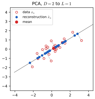
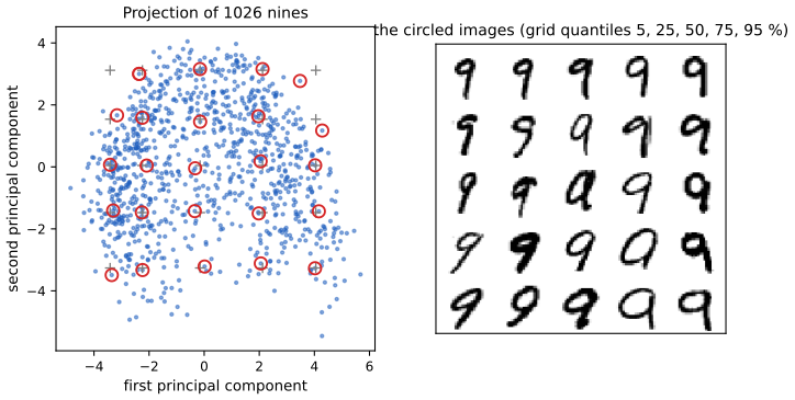
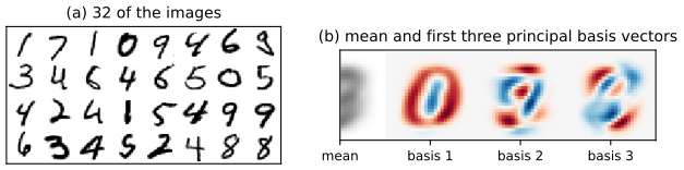
pp. 657–659 Figure 20.1 projects two-dimensional points onto the first principal axis. Figure 20.2 does the same for 1026 MNIST images of the digit 9 (784 pixels each): the first two components keep a quarter of the variance (25.3 percent), and the book reads the first component as the orientation of the digit and the second as the thickness of the line. Figure 20.3 shows the mean image and the first three principal basis vectors; these are the "eigenfaces" when the images are faces, and here (digits) the first one looks like a zero, the most common large-scale pattern. The pixels are strongly correlated, so a handful of directions carry much of the variation.
20.1.2 Derivation of the algorithm
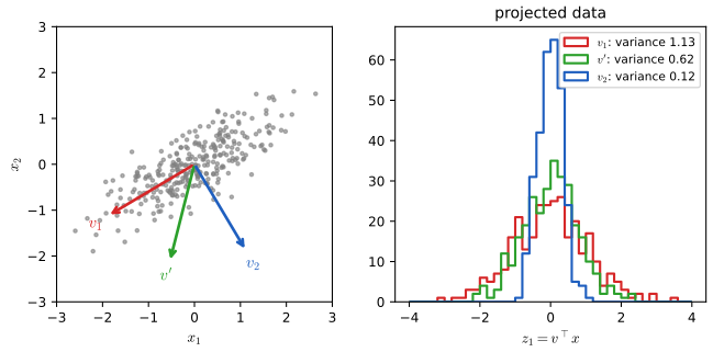
pp. 659–662 Assume the data are centred. Approximate each point as a combination of \(L\) orthonormal basis vectors, \(\bm x_n\approx\sum_{k=1}^Lz_{nk}\bm w_k=\bm W\bm z_n\), and measure the error by \[ \mathcal L(\bm W,\bm Z)=\frac1N\|\bm X-\bm Z\bm W^\T\|_F^2=\frac1N\sum_n\|\bm x_n-\bm W\bm z_n\|^2 . \tag{20.3} \] Base case (\(L=1\)). With \(\bm w_1^\T\bm w_1=1\), expanding the square gives \(\frac1N\sum_n[\bm x_n^\T\bm x_n-2z_{n1}\bm w_1^\T\bm x_n+z_{n1}^2]\) (20.6); setting the derivative in \(z_{n1}\) to zero gives \(z_{n1}=\bm w_1^\T\bm x_n\) (20.7), an orthogonal projection, and substituting back gives \(\mathcal L(\bm w_1)=\mathrm{const}-\bm w_1^\T\bm S\bm w_1\) (20.9). Maximising \(\bm w_1^\T\bm S\bm w_1\) under \(\|\bm w_1\|=1\) with a Lagrange multiplier gives \(\bm S\bm w_1=\lambda_1\bm w_1\) (20.12): \(\bm w_1\) is an eigenvector and the objective equals its eigenvalue (20.13), so the best choice is the top eigenvector. Variance view. Since the data are centred, \(\E[z_{n1}]=0\) and \(\var[\tilde z_1]=\frac1N\sum_nz_{n1}^2=-\mathcal L(\bm w_1)+\mathrm{const}\) (20.14, 20.15): minimising the reconstruction error is the same as maximising the variance of the projection (20.16), which is why PCA is said to find directions of maximal variance (Figure 20.4). Induction. The second direction \(\bm w_2\) is chosen with \(\bm w_2^\T\bm w_2=1\), \(\bm w_2^\T\bm w_1=0\); the error is \(\mathrm{const}-\bm w_2^\T\bm S\bm w_2\) (20.18), the Lagrangian (20.19) has stationary points at eigenvectors (20.20), and the second eigenvector is optimal. The proof continues to \(\hat{\bm W}=\bm U_L\). The book defers two steps to Exercise 20.3; Gap 20.1 proves the whole statement at once.
Filling the gap 20.1: the principal subspace is optimal for every \(L\) at once, and the error is \(\sum_{j>L}\lambda_j\) pp. 659–662, (20.1)–(20.20), Exercises 20.3 and 20.4
Proof
Setting. \(\bm X_c\) is centred, \(\bm S=\frac1N\bm X_c^\T\bm X_c=\sum_j\lambda_j\bm u_j\bm u_j^\T\) with orthonormal \(\bm u_j\) and \(\lambda_1\ge\dots\ge\lambda_D\ge0\). Minimise (20.3) over \(\bm W\in\R^{D\times L}\) with \(\bm W^\T\bm W=\bm I_L\) and \(\bm Z\in\R^{N\times L}\).
Step 1: the optimal codes (Exercise 20.3a). For fixed \(\bm W\), (20.3) is a sum over \(n\) of separate terms. Using \(\bm W^\T\bm W=\bm I\), \(\|\bm x_n-\bm W\bm z_n\|^2=\bm x_n^\T\bm x_n-2\bm z_n^\T\bm W^\T\bm x_n+\|\bm z_n\|^2\), a convex quadratic in \(\bm z_n\) with gradient \(-2\bm W^\T\bm x_n+2\bm z_n\); so \(\bm z_n=\bm W^\T\bm x_n\) (this contains (20.7) and the claim of Exercise 20.3a with \(\bm v_2\) in place of \(\bm w_2\)). The minimum value is \(\bm x_n^\T\bm x_n-\|\bm W^\T\bm x_n\|^2\), so \[ \mathcal L(\bm W)=\Tr(\bm S)-\Tr(\bm W^\T\bm S\bm W) . \]
Step 2: the maximum of \(\Tr(\bm W^\T\bm S\bm W)\) (Ky Fan). Let \(\bm P=\bm W\bm W^\T\), the orthogonal projector onto the column space of \(\bm W\); \(\Tr(\bm W^\T\bm S\bm W)=\Tr(\bm P\bm S)=\sum_j\lambda_jp_j\) with \(p_j=\bm u_j^\T\bm P\bm u_j=\|\bm W^\T\bm u_j\|^2\). Because \(\bm P\preceq\bm I\), \(0\le p_j\le1\), and \(\sum_jp_j=\Tr\bm P=L\). Then \[ \sum_j\lambda_jp_j-\sum_{j\le L}\lambda_j=\sum_{j\le L}\lambda_j(p_j-1)+\sum_{j>L}\lambda_jp_j\le\lambda_L\sum_{j\le L}(p_j-1)+\lambda_L\sum_{j>L}p_j=\lambda_L\Big(\sum_jp_j-L\Big)=0 , \] because \(p_j-1\le0\) and \(\lambda_j\ge\lambda_L\) for \(j\le L\), while \(p_j\ge0\) and \(\lambda_j\le\lambda_L\) for \(j>L\). So \(\Tr(\bm W^\T\bm S\bm W)\le\sum_{j\le L}\lambda_j\), with equality for \(\bm W=\bm U_L\) (or any \(\bm U_L\bm R\) with \(\bm R\) orthogonal). If \(\lambda_L>\lambda_{L+1}\), equality forces \(p_j=1\) for \(j\le L\) and \(p_j=0\) for \(j>L\), i.e. \(\bm u_j\in\mathrm{span}(\bm W)\) for \(j\le L\): the optimal subspace is unique, and the basis is unique only up to a rotation inside it (and signs, and ordering by eigenvalue in the book's convention).
Step 3: the error (Exercise 20.4). Hence the minimum of (20.3) is \[ \mathcal L_L=\Tr(\bm S)-\sum_{j\le L}\lambda_j=\sum_{j=L+1}^D\lambda_j , \tag{20.26} \] since \(\Tr\bm S=\sum_{j\le D}\lambda_j\). This is the argument of Exercise 20.4: (a) \(\|\bm x-\sum_jz_j\bm v_j\|^2=\bm x^\T\bm x-\sum_jz_j^2\) for orthonormal \(\bm v_j\) and \(z_j=\bm v_j^\T\bm x\) (expand the square and use \(\bm v_j^\T\bm v_k=\delta_{jk}\)); (b) averaging, \(\frac1N\sum_n(\bm x_n^\T\bm x_n-\sum_j\bm v_j^\T\bm x_n\bm x_n^\T\bm v_j)=\Tr\bm S-\sum_j\bm v_j^\T\bm S\bm v_j=\Tr\bm S-\sum_{j\le K}\lambda_j\) for eigenvectors \(\bm v_j\); (c) for \(K=D\) there is no truncation, the error is 0, so \(\Tr\bm S=\sum_{j\le D}\lambda_j\), and subtracting gives the tail sum. In terms of the SVD \(\bm X_c=\bm U_X\bm S_X\bm V_X^\T\), \(\lambda_j=s_j^2/N\).
Step 4: the greedy construction of the book (Exercise 20.3b). Let \(\bm w_1=\bm u_1\) be fixed. For \(\bm w_2\) minimise \(-\bm w_2^\T\bm S\bm w_2+\lambda_2'(\bm w_2^\T\bm w_2-1)+\lambda_{12}\bm w_2^\T\bm w_1\) (the book's (20.19) with Lagrange multipliers \(\lambda_2'\), \(\lambda_{12}\)). The gradient is \(-2\bm S\bm w_2+2\lambda_2'\bm w_2+\lambda_{12}\bm w_1=0\). Multiplying by \(\bm w_1^\T\) and using \(\bm w_1^\T\bm S=\lambda_1\bm w_1^\T\) and \(\bm w_1^\T\bm w_2=0\) gives \(-2\lambda_1\cdot0+0+\lambda_{12}=0\), so \(\lambda_{12}=0\) and \(\bm S\bm w_2=\lambda_2'\bm w_2\): \(\bm w_2\) is an eigenvector orthogonal to \(\bm u_1\), with objective value \(\lambda_2'\), maximal for the second eigenvalue. By Step 2 the greedy solution is also the global optimum for \(L=2\), and likewise for every \(L\). A numerical experiment in three dimensions (scanning all unit vectors orthogonal to \(\bm u_1\)) confirms that the second eigenvector maximises the variance, with value \(\lambda_2\), and that no random orthonormal basis of 300 tried beats \(\bm U_L\) on the digits data. \(\square\)
20.1.3 Computational issues
20.1.3.1 Covariance matrix vs correlation matrix
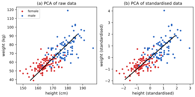
p. 662 PCA of the covariance matrix is not invariant to the units of the features: a feature measured in grams instead of kilograms has a variance a million times larger and swallows the first component. Standardising each column to mean 0 and variance 1, which is the same as taking the eigenvectors of the correlation matrix, removes the dependence on units. Figure 20.5: on the height and weight data the first axis of the raw data points at 59 degrees from the height axis (weight dominates, variance 232 against 25), but after standardising it sits at exactly 45 degrees (two features with equal variance, correlation 0.77, eigenvalues \(1\pm0.77\)).
Filling the gap 20.2: covariance PCA depends on the scale of the features, correlation PCA does not p. 662
Proof
Let \(\bm x'=\bm D\bm x\) with \(\bm D=\diag(d_1,\dots,d_D)\), \(d_j>0\), a change of units. The covariance becomes \(\bm S'=\bm D\bm S\bm D\), which is generally not similar to \(\bm S\) by an orthogonal transformation, so the eigenvectors of \(\bm S'\) are not the rescaled eigenvectors of \(\bm S\): for example with \(\bm S=\begin{pmatrix}1&r\\r&1\end{pmatrix}\) and \(\bm D=\diag(1,d)\), \(\bm S'=\begin{pmatrix}1&rd\\rd&d^2\end{pmatrix}\) has first eigenvector tending to \((0,1)\) as \(d\to\infty\) whatever \(r\ne0\) is. The standardised variables are \(\tilde x_j=(x_j-\mu_j)/\sqrt{S_{jj}}\), and \(S'_{jj}=d_j^2S_{jj}\), so \(\tilde x'_j=(d_jx_j-d_j\mu_j)/(d_j\sqrt{S_{jj}})=\tilde x_j\): the standardised data, hence their covariance \(\bm R=\bm S_{\rm diag}^{-1/2}\bm S\bm S_{\rm diag}^{-1/2}\) (the correlation matrix) and its eigendecomposition, are unchanged by any such \(\bm D\). With two standardised features and correlation \(r\), \(\bm R=\begin{pmatrix}1&r\\r&1\end{pmatrix}\) has eigenvalues \(1\pm r\) and eigenvectors \((1,\pm1)/\sqrt2\) for every \(r>0\): the first axis is the diagonal at 45 degrees, as in Figure 20.5b (\(r=0.771\), eigenvalues 1.771 and 0.229). The price of standardising is that PCA then explains the correlation structure, not the original variances, and a feature of pure noise is given as much weight as an informative one. \(\square\)
20.1.3.2 Dealing with high-dimensional data
p. 663 If \(D>N\) the \(D\times D\) covariance is expensive but rank at most \(N-1\), and it is cheaper to diagonalise the \(N\times N\) Gram matrix \(\bm X_c\bm X_c^\T\). If \(\bm X_c\bm X_c^\T\bm U=\bm U\bm\Lambda\) then \((\bm X_c^\T\bm X_c)(\bm X_c^\T\bm U)=(\bm X_c^\T\bm U)\bm\Lambda\) (20.21): the columns of \(\bm X_c^\T\bm U\) are eigenvectors of \(\bm X_c^\T\bm X_c\) with the same eigenvalues, but of squared length \(\lambda_j\), so the unit eigenvectors are \(\bm V=\bm X_c^\T\bm U\bm\Lambda^{-1/2}\) (20.22). (The eigenvalues of \(\bm S\) are \(\lambda_j/N\); the book's \(\bm\Lambda\) here is that of the Gram matrix.) This is also the route that lets us replace inner products by kernels in Section 20.4.6.
20.1.3.3 Computing PCA using SVD
p. 663 With the thin SVD \(\bm X_c=\bm U_X\bm S_X\bm V_X^\T\), \(\bm X_c^\T\bm X_c=\bm V_X\bm S_X^2\bm V_X^\T\), so the right singular vectors are the principal axes, \(\bm W=\bm V_X\) (first \(L\) columns), the eigenvalues are \(\lambda_k=s_k^2/N\), the scores are \(\bm Z=\bm X_c\bm W=\bm U_X\bm S_X\) (20.23) and the reconstruction \(\hat{\bm X}=\bm Z\bm W^\T=\bm U_X\bm S_X\bm V_X^\T\) is the truncated SVD of Section 7.5.5 (20.24). The SVD route avoids forming \(\bm X_c^\T\bm X_c\), whose condition number is the square of that of \(\bm X_c\), and randomised SVD gives the top \(L\) components in \(O(NL^2)+O(L^3)\) time (after the random projection) instead of \(O(ND^2)+O(D^3)\).
Filling the gap 20.3: three routes to the same PCA, and why the SVD route is the stable one pp. 663–664, (20.21)–(20.24)
Derivation
Gram route. Let \(\bm G=\bm X_c\bm X_c^\T=\bm U\bm\Lambda\bm U^\T\), with \(\lambda_j>0\) for \(j\le r=\mathrm{rank}\,\bm X_c\). For \(\bm v_j=\bm X_c^\T\bm u_j\): \(\bm X_c^\T\bm X_c\bm v_j=\bm X_c^\T\bm G\bm u_j=\lambda_j\bm X_c^\T\bm u_j=\lambda_j\bm v_j\), and \(\|\bm v_j\|^2=\bm u_j^\T\bm X_c\bm X_c^\T\bm u_j=\lambda_j\). Dividing by \(\sqrt{\lambda_j}\) gives unit eigenvectors (20.22); different \(j\) give orthogonal \(\bm v_j\) since \(\bm v_j^\T\bm v_k=\bm u_j^\T\bm G\bm u_k=\lambda_k\delta_{jk}\). All \(r\) non-zero eigenpairs of \(\bm X_c^\T\bm X_c\) are obtained this way. Cost \(O(N^2D+N^3)\) against \(O(ND^2+D^3)\).
SVD route. If \(\bm X_c=\bm U_X\bm S_X\bm V_X^\T\), the Gram eigenvectors are \(\bm U_X\) with eigenvalues \(s_j^2\), and (20.22) returns \(\bm V=\bm X_c^\T\bm U_X\bm S_X^{-1}=\bm V_X\bm S_X\bm U_X^\T\bm U_X\bm S_X^{-1}=\bm V_X\): the three routes agree. Condition numbers: \(\kappa(\bm X_c^\T\bm X_c)=\kappa(\bm X_c)^2\), so small singular values (the trailing components) are determined with absolute error about \(\epsilon\,s_1^2\) from the covariance but \(\epsilon\,s_1\) from the SVD, a relative accuracy of \(s_1/s_j\) times better.
All three were run on the UCI digits: the eigenvalues of the covariance, the values \(s_j^2/N\) of the SVD and the Gram-matrix values divided by \(N\) agree to 9 digits, the eigenvectors agree up to sign, the Gram basis has unit norms, and scikit-learn's PCA returns the same components with eigenvalues scaled by \(N/(N-1)\) (it divides by \(N-1\)). \(\square\)
20.1.4 Choosing the number of latent dimensions
20.1.4.1 Reconstruction error
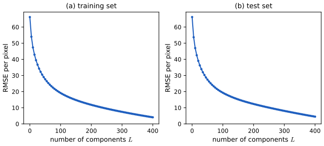
p. 664 The reconstruction error on a data set \(\mathcal D\) with \(L\) components is \(\mathcal L_L=\frac1{|\mathcal D|}\sum_{n\in\mathcal D}\|\bm x_n-\hat{\bm x}_n\|^2\), with \(\hat{\bm x}_n=\bm W\bm z_n+\bm\mu\), \(\bm z_n=\bm W^\T(\bm x_n-\bm\mu)\) (20.25). On the training set it falls to zero at \(L=\mathrm{rank}\,\bm X\) (Figure 20.6a). On a held-out set it keeps falling (Figure 20.6b): there is no U shape, because PCA is not a generative model whose likelihood can be overfitted. Gap 20.4 shows that this is a theorem, not an accident.
20.1.4.2 Scree plots
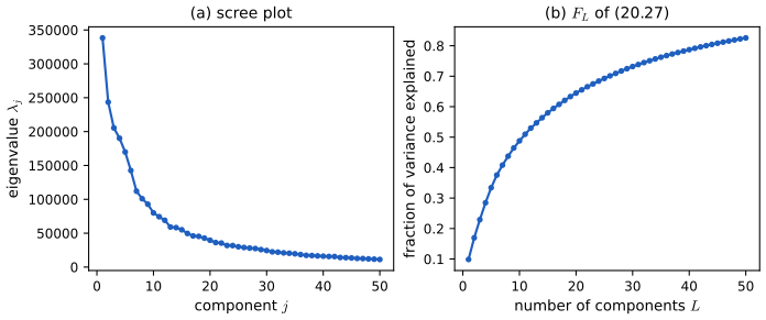
pp. 664–665 A scree plot shows the eigenvalues \(\lambda_j\) against \(j\); by (20.26) the training error at \(L\) is the area under the plot to the right of \(L\). The fraction of variance explained is \[ F_L=\frac{\sum_{j\le L}\lambda_j}{\sum_{j'\le L_{\max}}\lambda_{j'}} , \tag{20.27} \] which rises with \(L\) (Figure 20.7). On the MNIST sample \(F_{10}=0.49\), \(F_{50}=0.83\), and 86 components are needed for 90 percent and 150 for 95 percent.
Filling the gap 20.4: held-out reconstruction error is non-increasing in \(L\), and the training error is the tail sum pp. 664–665, (20.25), (20.26)
Proof
Fix any orthonormal basis \(\bm u_1,\bm u_2,\dots\) (the eigenvectors of a training covariance) and the training mean \(\bm\mu\). For any point \(\bm x\) (training or not) with \(\bm c=\bm x-\bm\mu\), the reconstruction from the first \(L\) components is \(\hat{\bm x}_L=\bm\mu+\sum_{j\le L}(\bm u_j^\T\bm c)\bm u_j\), an orthogonal projection of \(\bm c\), so by Pythagoras \[ \|\bm x-\hat{\bm x}_L\|^2=\|\bm c\|^2-\sum_{j\le L}(\bm u_j^\T\bm c)^2 , \] which is non-increasing in \(L\) for every \(\bm x\). Averaging over a held-out set preserves this: the test error \(\mathcal L_L^{\rm test}=\overline{\|\bm c\|^2}-\sum_{j\le L}\overline{(\bm u_j^\T\bm c)^2}\) is non-increasing, strictly decreasing unless every test point is orthogonal to \(\bm u_L\). The data enter only through the basis, so there is nothing to overfit in the sense of a model that fits the training noise at the cost of test performance: a projection never makes a point worse. On the training set \(\overline{(\bm u_j^\T\bm c)^2}=\bm u_j^\T\bm S\bm u_j=\lambda_j\), which gives \(\mathcal L_L=\sum_{j>L}\lambda_j\) (20.26) again, and on the test set the decrements \(\overline{(\bm u_j^\T\bm c)^2}\) are positive but not ordered, because the basis is optimal for the training covariance only. (Numerically, on the MNIST sample the test error decreased at every one of 30 tested values of \(L\), and the training curve matched the tail sums of the eigenvalues to 8 digits.) The held-out likelihood of the probabilistic version behaves differently: for PPCA fitted to 600 digits (60 non-constant pixels) and evaluated on 400 others, the mean log likelihood rose steadily from \(-172\) at \(L=1\) to \(-122\) at \(L=55\), then fell by 15 nats at \(L=58\), where the noise variance is estimated from only two tiny eigenvalues: overfitting shows up near full rank, not in the middle. The relevant lesson: the reconstruction error of PCA cannot select \(L\); a quantity that can rise is the error against the clean signal when the data contain noise (the demonstration below), or the held-out log likelihood of a probabilistic model (Section 20.2.2).
The fraction of variance explained is \(F_L=1-\mathcal L_L/\Tr\bm S\) when \(L_{\max}=D\), so (20.27) and the scree plot carry the same information as the error curve. \(\square\)
20.1.4.3 Profile likelihood
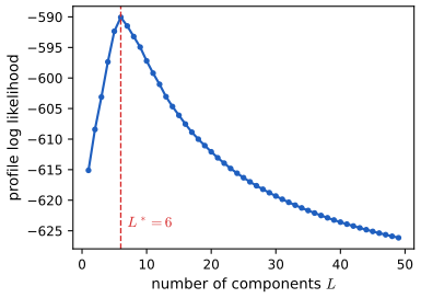
pp. 665–666 A knee in the scree plot can be located automatically (Zhu and Ghodsi, 2006). Split the decreasing sequence \(\lambda_1\ge\dots\ge\lambda_{L_{\max}}\) at \(L\): model the first \(L\) values as i.i.d. \(\N(\mu_1,\sigma^2)\) and the rest as i.i.d. \(\N(\mu_2,\sigma^2)\), with a common variance. The maximum likelihood estimates are \[ \mu_1(L)=\frac{\sum_{k\le L}\lambda_k}L,\quad\mu_2(L)=\frac{\sum_{k>L}\lambda_k}{L_{\max}-L},\quad \sigma^2(L)=\frac{\sum_{k\le L}(\lambda_k-\mu_1)^2+\sum_{k>L}(\lambda_k-\mu_2)^2}{L_{\max}} , \tag{20.28–20.30} \] and the profile log likelihood is \(\ell(L)=\sum_{k\le L}\log\N(\lambda_k\given\mu_1(L),\sigma^2(L))+\sum_{k>L}\log\N(\lambda_k\given\mu_2(L),\sigma^2(L))\) (20.31); take \(L^*=\arg\max\ell(L)\) (Figure 20.8; the data are not i.i.d., but the device works).
Filling the gap 20.5: the maximum likelihood estimates of the change-point model, and a closed form for the profile likelihood pp. 665–666, (20.28)–(20.31)
Derivation
For fixed \(L\) the likelihood of \(\lambda_1,\dots,\lambda_{L_{\max}}\) is \(\prod_{k\le L}\N(\lambda_k\given\mu_1,\sigma^2)\prod_{k>L}\N(\lambda_k\given\mu_2,\sigma^2)\), so \[ \ell(\mu_1,\mu_2,\sigma^2)=-\tfrac{L_{\max}}2\log(2\pi\sigma^2)-\frac1{2\sigma^2}\Big[\sum_{k\le L}(\lambda_k-\mu_1)^2+\sum_{k>L}(\lambda_k-\mu_2)^2\Big] . \] The bracket is the sum of two separate squared errors, minimised over \(\mu_1\) and \(\mu_2\) by the group means (20.28, 20.29) for every \(\sigma^2>0\). Writing \(Q(L)\) for the minimised bracket, \(\partial_{\sigma^2}\ell=-\frac{L_{\max}}{2\sigma^2}+\frac{Q}{2\sigma^4}=0\) gives \(\sigma^2=Q/L_{\max}\), (20.30): one pooled variance, as the book requires "to prevent overfitting when one regime has less data". Inserting the estimates, the quadratic term equals \(-\frac{Q}{2\sigma^2}=-\frac{L_{\max}}2\), so \[ \ell(L)=-\frac{L_{\max}}2\Big(\log\big(2\pi\sigma^2(L)\big)+1\Big) , \] a decreasing function of the pooled variance \(\sigma^2(L)\): the best split is the one for which the two-level step function fits the eigenvalue sequence with the smallest residual sum of squares, and \(L^*\) is the "knee" in exactly that least-squares sense. This closed form agrees to machine precision with the direct sum (20.31) for the MNIST eigenvalues, and a numerical optimiser over \((\mu_1,\mu_2,\log\sigma)\) returns the estimates (20.28)–(20.30). The same device applies to any decreasing error sequence, for instance the distortion of \(K\)-means as the number of clusters grows (Section 21.3.7). \(\square\)
20.2 Factor analysis
pp. 666–679 Factor analysis (FA) is a probabilistic model of the same low-dimensional structure. Because it is a model, it can be a building block (mixtures, nonlinear versions, missing data) and PCA appears as a limiting case.
See also: Bayesian and Probabilistic ML, Section 12.2; Foundations of Deep Learning, Section 16.2.
20.2.1 Generative model
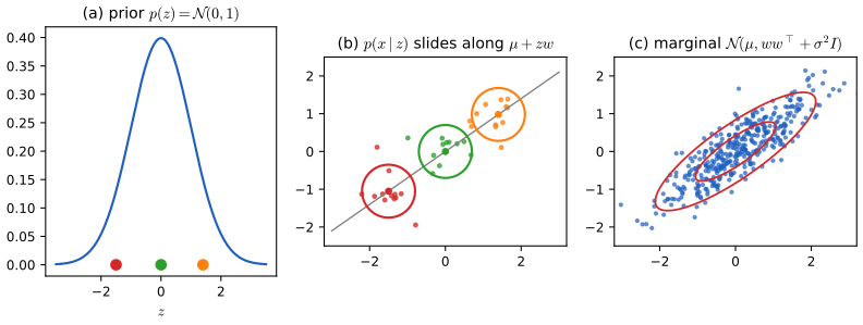
pp. 667–668 The model is linear and Gaussian: \[ p(\bm z)=\N(\bm z\given\bm\mu_0,\bm\Sigma_0),\qquad p(\bm x\given\bm z,\bm\theta)=\N(\bm x\given\bm W\bm z+\bm\mu,\bm\Psi), \tag{20.32, 20.33} \] with the factor loading matrix \(\bm W\in\R^{D\times L}\) and a diagonal \(\bm\Psi\). The marginal is Gaussian, \(p(\bm x)=\N(\bm x\given\bm W\bm\mu_0+\bm\mu,\ \bm\Psi+\bm W\bm\Sigma_0\bm W^\T)\) (20.34, 20.35), so we may take \(\bm\mu_0=\bm 0\) and \(\bm\Sigma_0=\bm I\) without loss of generality (20.36–20.38): \[ p(\bm x)=\N(\bm x\given\bm\mu,\bm C),\qquad\bm C=\bm W\bm W^\T+\bm\Psi . \tag{20.38, 20.39} \] FA is a low-rank-plus-diagonal Gaussian: it has \(O(LD)\) parameters, between the \(O(D^2)\) of a full covariance and the \(O(D)\) of a diagonal one. \(\bm\Psi\) must be diagonal: with a full \(\bm\Psi\) one could take \(\bm W=\bm 0\) and fit any covariance, so the latent factors would be unused. The variance of coordinate \(d\) is \(\sum_kw_{dk}^2+\psi_d\), the communality (variance due to the common factors) plus the uniqueness \(\psi_d\). The posterior over the factors is \[ p(\bm z\given\bm x)=\N\big(\bm z\given\bm W^\T\bm C^{-1}(\bm x-\bm\mu),\ \bm I-\bm W^\T\bm C^{-1}\bm W\big) . \tag{20.40} \] Figure 20.9 shows the picture for \(L=1\), \(D=2\), \(\bm\Psi=\sigma^2\bm I\): the isotropic "spray can" \(p(\bm x\given z)\) slides along the line \(\bm\mu+z\bm w\) as \(z\) varies, producing an elongated Gaussian.
Filling the gap 20.6: the FA marginal, the reduction to \(\bm\mu_0=\bm 0\), \(\bm\Sigma_0=\bm I\), and the two forms of the posterior pp. 667–668, (20.34)–(20.40)
Derivation
Marginal. Write \(\bm x=\bm W\bm z+\bm\mu+\bm\epsilon\) with \(\bm z\sim\N(\bm\mu_0,\bm\Sigma_0)\) and \(\bm\epsilon\sim\N(\bm 0,\bm\Psi)\) independent. A linear combination of independent Gaussians is Gaussian; its mean is \(\bm W\bm\mu_0+\bm\mu\) and its covariance \(\bm W\bm\Sigma_0\bm W^\T+\bm\Psi\) (this is the linear Gaussian system of Section 3.3, (3.38)). The reductions. Put \(\bm z=\bm\mu_0+\bm\Sigma_0^{1/2}\bm z'\) with \(\bm z'\sim\N(\bm 0,\bm I)\); then \(\bm W\bm z+\bm\mu=(\bm W\bm\Sigma_0^{1/2})\bm z'+(\bm\mu+\bm W\bm\mu_0)\), so the model with \((\bm\mu_0,\bm\Sigma_0,\bm W,\bm\mu)\) equals the model with \((\bm 0,\bm I,\tilde{\bm W},\tilde{\bm\mu})\) where \(\tilde{\bm W}=\bm W\bm\Sigma_0^{1/2}\) and \(\tilde{\bm\mu}=\bm\mu+\bm W\bm\mu_0\) (the book writes the exponent as \(-\frac12\); with that sign the covariance would be \(\bm W\bm\Sigma_0^{-1}\bm W^\T\), which is not \(\bm W\bm\Sigma_0\bm W^\T\)).
Posterior, Gaussian-conditioning form. The pair \((\bm z,\bm x)\) is jointly Gaussian with \(\mathrm{cov}(\bm z,\bm x)=\E[\bm z(\bm W\bm z+\bm\epsilon)^\T]=\bm W^\T\), \(\mathrm{cov}(\bm x)=\bm C\) and \(\mathrm{cov}(\bm z)=\bm I\). Conditioning (Section 3.2.3) gives mean \(\bm W^\T\bm C^{-1}(\bm x-\bm\mu)\) and covariance \(\bm I-\bm W^\T\bm C^{-1}\bm W\): this is (20.40).
Posterior, information form. By Bayes' rule, \(\log p(\bm z\given\bm x)=-\frac12\|\bm z\|^2-\frac12(\bm x-\bm\mu-\bm W\bm z)^\T\bm\Psi^{-1}(\bm x-\bm\mu-\bm W\bm z)+\mathrm{const}\), a quadratic in \(\bm z\) with precision \(\bm I+\bm W^\T\bm\Psi^{-1}\bm W\) and linear term \(\bm W^\T\bm\Psi^{-1}(\bm x-\bm\mu)\), so \(p(\bm z\given\bm x)=\N(\bm m,\bm\Sigma)\) with \(\bm\Sigma=(\bm I+\bm W^\T\bm\Psi^{-1}\bm W)^{-1}\) and \(\bm m=\bm\Sigma\bm W^\T\bm\Psi^{-1}(\bm x-\bm\mu)\) (20.55, 20.56). This costs an \(L\times L\) inverse instead of a \(D\times D\) one. The two forms agree. The identity \((\bm I+\bm W^\T\bm\Psi^{-1}\bm W)\bm W^\T=\bm W^\T\bm\Psi^{-1}(\bm\Psi+\bm W\bm W^\T)\) (expand both sides) gives \((\bm I+\bm W^\T\bm\Psi^{-1}\bm W)^{-1}\bm W^\T\bm\Psi^{-1}=\bm W^\T\bm C^{-1}\), so the means agree; and the Woodbury identity gives \((\bm I+\bm W^\T\bm\Psi^{-1}\bm W)^{-1}=\bm I-\bm W^\T(\bm\Psi+\bm W\bm W^\T)^{-1}\bm W\), so the covariances agree. Both forms were compared numerically on a random \(D=6\), \(L=2\) model, and the sample covariance of \(4\times10^5\) draws matched \(\bm W\bm W^\T+\bm\Psi\). \(\square\)
20.2.2 Probabilistic PCA
pp. 668–669 Probabilistic PCA (PPCA; Tipping and Bishop, 1999) or sensible PCA (Roweis, 1997) is the special case \(\bm\Psi=\sigma^2\bm I\) with orthonormal columns of \(\bm W\) (the orthonormality is not needed for the likelihood; see below). The marginal is \(\N(\bm\mu,\bm C)\) with \(\bm C=\bm W\bm W^\T+\sigma^2\bm I\) (20.41, 20.42), and with \(\hat{\bm\mu}=\bar{\bm x}\) the log likelihood is \[ \log p(\bm X\given\bm\mu,\bm W,\sigma^2)=-\frac N2\Big(D\log2\pi+\log|\bm C|+\Tr(\bm C^{-1}\bm S)\Big) . \tag{20.43, 20.44} \] Tipping and Bishop (1999) and Roweis (1997) show that the maximum satisfies \[ \bm W=\bm U_L(\bm\Lambda_L-\sigma^2\bm I)^{1/2}\bm R,\qquad\sigma^2=\frac1{D-L}\sum_{i=L+1}^D\lambda_i , \tag{20.45, 20.46} \] with \(\bm R\) an arbitrary orthogonal matrix (take \(\bm I\)), \(\bm\Lambda_L=\diag(\lambda_1,\dots,\lambda_L)\); as \(\sigma^2\to0\), \(\bm W\to\bm U_L\bm\Lambda_L^{1/2}\), proportional to the PCA basis. The noise is the average variance in the discarded directions. For evaluating the density, the matrix-inversion lemma gives \(\bm C^{-1}=\sigma^{-2}(\bm I-\bm W\bm M^{-1}\bm W^\T)\) with \(\bm M=\bm W^\T\bm W+\sigma^2\bm I\) (\(L\times L\)) (20.47, 20.48); at the maximum \(\bm M=\bm\Lambda_L\) so \(\bm C^{-1}=\sigma^{-2}\big(\bm I-\bm U_L(\bm\Lambda_L-\sigma^2\bm I)\bm\Lambda_L^{-1}\bm U_L^\T\big)\) (20.50) and \(\log|\bm C|=(D-L)\log\sigma^2+\sum_{j\le L}\log\lambda_j\) (20.51): no matrix inversion is needed. The posterior (the encoder) is \[ p(\bm z\given\bm x)=\N\big(\bm z\given\bm M^{-1}\bm W^\T(\bm x-\bm\mu),\ \sigma^2\bm M^{-1}\big) , \tag{20.52} \] which in the limit \(\sigma^2\to0\) has the mean \((\bm W^\T\bm W)^{-1}\bm W^\T(\bm x-\bar{\bm x})\), the orthogonal projection of PCA (20.53).
Filling the gap 20.7: the maximum likelihood estimate of probabilistic PCA is the global maximum; efficient formulas pp. 668–669, (20.43)–(20.53), Exercises 20.6, 20.7, 20.9
Proof
Claim. Let \(\bm S=\sum_j\lambda_j\bm u_j\bm u_j^\T\) have eigenvalues \(\lambda_1\ge\dots\ge\lambda_D>0\). Over all \(\bm W\in\R^{D\times L}\) and \(\sigma^2>0\), \(f(\bm W,\sigma^2)=\log|\bm C|+\Tr(\bm C^{-1}\bm S)\) is minimised (the likelihood is maximised) by (20.45)–(20.46); the solution is unique up to \(\bm W\mapsto\bm W\bm R\) when \(\lambda_L>\lambda_{L+1}\). The mean estimate \(\hat{\bm\mu}=\bar{\bm x}\) follows by setting the gradient of \(\sum_n(\bm x_n-\bm\mu)^\T\bm C^{-1}(\bm x_n-\bm\mu)\) to zero, and then \(\frac1N\sum_n(\bm x_n-\bar{\bm x})^\T\bm C^{-1}(\bm x_n-\bar{\bm x})=\Tr(\bm C^{-1}\bm S)\) gives (20.44).
Step 1: reduce to the eigenvalues of \(\bm C\). Let \(c_1\ge\dots\ge c_D\) be the eigenvalues of \(\bm C=\bm W\bm W^\T+\sigma^2\bm I\). Since \(\bm W\bm W^\T\) is positive semi-definite of rank at most \(L\), every \(c_i\ge\sigma^2\) and \(c_i=\sigma^2\) for at least \(D-L\) indices. We have \(\log|\bm C|=\sum_i\log c_i\). By the von Neumann trace inequality, for symmetric matrices \(\Tr(\bm A\bm B)\ge\sum_ia_i^\uparrow b_i^\downarrow\) (eigenvalues of one in ascending order paired with those of the other in descending order), applied to \(\bm A=\bm C^{-1}\) (ascending eigenvalues \(1/c_1\le\dots\le1/c_D\)) and \(\bm B=\bm S\): \(\Tr(\bm C^{-1}\bm S)\ge\sum_i\lambda_i/c_i\). Hence \[ f\ge\sum_{i=1}^Dh_i(c_i),\qquad h_i(c)=\log c+\frac{\lambda_i}{c} , \] with equality when \(\bm C\) has eigenvector \(\bm u_i\) for eigenvalue \(c_i\) (then \(\bm C\) and \(\bm S\) commute and are diagonal in the same basis).
Step 2: relax and minimise. The function \(h_i\) on \(c>0\) has derivative \(1/c-\lambda_i/c^2\), so it is minimised at \(c=\lambda_i\) with value \(\log\lambda_i+1\). Fix \(\sigma^2\) and relax the constraints: let \(c_1,\dots,c_L>0\) be free (no ordering, no \(c\ge\sigma^2\)) and \(c_i=\sigma^2\) for \(i>L\). Then \[ \sum_ih_i(c_i)\ge G(\sigma^2):=\sum_{i\le L}(\log\lambda_i+1)+(D-L)\log\sigma^2+\frac1{\sigma^2}\sum_{i>L}\lambda_i . \] (A relaxed minimum is at most the constrained one, so this inequality holds for every feasible \(\bm C\).) \(G\) has \(G'(\sigma^2)=\frac{D-L}{\sigma^2}-\frac{1}{\sigma^4}\sum_{i>L}\lambda_i\), which vanishes only at \(\sigma_*^2=\frac1{D-L}\sum_{i>L}\lambda_i\), where \(G\) attains its minimum (it decreases before and increases after). This is (20.46).
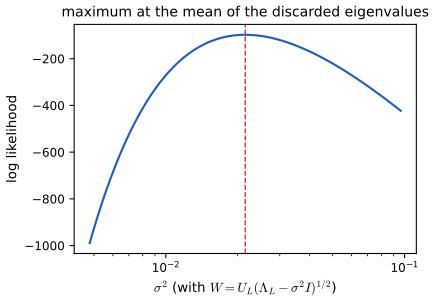
Step 3: the bound is attained. Since \(\sigma_*^2\) is the mean of \(\lambda_{L+1},\dots,\lambda_D\), \(\sigma_*^2\le\lambda_{L+1}\le\lambda_L\), so the choice \(c_i=\lambda_i\) (\(i\le L\)), \(c_i=\sigma_*^2\) (\(i>L\)), with eigenvectors \(\bm u_i\), satisfies all the constraints: \(\bm C=\sigma_*^2\bm I+\bm U_L(\bm\Lambda_L-\sigma_*^2\bm I)\bm U_L^\T\), i.e. \(\bm W\bm W^\T=\bm U_L(\bm\Lambda_L-\sigma_*^2\bm I)\bm U_L^\T\). Any \(\bm W\) with this product equals \(\bm U_L(\bm\Lambda_L-\sigma_*^2\bm I)^{1/2}\bm R\) for an orthogonal \(\bm R\) (two matrices with the same Gram matrix \(\bm W\bm W^\T\) differ by a right orthogonal factor). So the lower bound \(G(\sigma_*^2)\) is reached, and (20.45)–(20.46) is a global maximum. Its value is \(-\frac N2\big(D\log2\pi+\sum_{j\le L}\log\lambda_j+(D-L)\log\sigma_*^2+D\big)\), since \(\Tr(\bm C^{-1}\bm S)=L+\frac1{\sigma_*^2}\sum_{i>L}\lambda_i=D\). A numerical experiment: the gradient of the log likelihood at the closed form vanishes, an L-BFGS search from a random start does not beat it, and the profile in \(\sigma^2\) (Figure 20.S2) peaks at \(\sigma_*^2\). If \(L=D\) the noise is 0 and the model reproduces \(\bm S\) exactly.
Efficient formulas. (i) \((\sigma^2\bm I+\bm W\bm W^\T)(\bm I-\bm W\bm M^{-1}\bm W^\T)=\sigma^2\bm I+\bm W\bm W^\T-\bm W(\sigma^2\bm I+\bm W^\T\bm W)\bm M^{-1}\bm W^\T=\sigma^2\bm I\), so \(\bm C^{-1}=\sigma^{-2}(\bm I-\bm W\bm M^{-1}\bm W^\T)\) (20.47). (ii) \(|\bm C|=\sigma^{2D}|\bm I_L+\sigma^{-2}\bm W^\T\bm W|=\sigma^{2(D-L)}|\bm M|\) (determinant lemma). At the maximum \(\bm W^\T\bm W=\bm\Lambda_L-\sigma^2\bm I\), so \(\bm M=\bm\Lambda_L\) (the book's (20.49) shows the \(D\times D\) matrix \(\bm U_L(\bm\Lambda_L-\sigma^2\bm I)\bm U_L^\T+\sigma^2\bm I\), which is \(\bm C\), not the \(L\times L\) matrix \(\bm M\)), giving (20.50) and (20.51). (iii) The posterior (20.52) is (20.40) with \(\bm\Psi=\sigma^2\bm I\), written in the information form of Gap 20.6: precision \(\bm I+\sigma^{-2}\bm W^\T\bm W=\sigma^{-2}\bm M\). (iv) Exercise 20.6: for a unit vector \(\bm v\), \(\bm v^\T\bm C\bm v=\|\bm W^\T\bm v\|^2+\sigma^2\). If \(\bm v\perp\mathrm{span}(\bm U_L)\) then \(\bm W^\T\bm v=\bm 0\) and \(\bm v^\T\bm C\bm v=\sigma^2\); if \(\bm v=\bm u_i\), \(i\le L\), then \(\bm W^\T\bm u_i=(\lambda_i-\sigma^2)^{1/2}\bm R^\T\bm e_i\) so \(\bm v^\T\bm C\bm v=(\lambda_i-\sigma^2)+\sigma^2=\lambda_i\): the model reproduces the variance along each principal axis exactly and spreads the rest evenly. \(\square\)
20.2.3 EM algorithm for FA/PPCA
20.2.3.1 EM for FA
p. 670 The E step computes the posterior \(p(\bm z_i\given\bm x_i,\bm\theta)=\N(\bm m_i,\bm\Sigma_i)\) with \(\bm\Sigma_i=(\bm I_L+\bm W^\T\bm\Psi^{-1}\bm W)^{-1}\) and \(\bm m_i=\bm\Sigma_i\bm W^\T\bm\Psi^{-1}(\bm x_i-\bm\mu)\) (20.54–20.56). For the M step, absorb the mean: \(\tilde{\bm W}=(\bm W,\bm\mu)\), \(\tilde{\bm z}=(\bm z,1)\), \(\bm b_i=\E[\tilde{\bm z}\given\bm x_i]=(\bm m_i;1)\), \(\bm C_i=\E[\tilde{\bm z}\tilde{\bm z}^\T\given\bm x_i]=\begin{pmatrix}\bm\Sigma_i+\bm m_i\bm m_i^\T&\bm m_i\\\bm m_i^\T&1\end{pmatrix}\) (20.57, 20.58), and update \[ \hat{\tilde{\bm W}}=\Big[\sum_i\bm x_i\bm b_i^\T\Big]\Big[\sum_i\bm C_i\Big]^{-1},\qquad\hat{\bm\Psi}=\frac1N\diag\Big\{\sum_i(\bm x_i-\hat{\tilde{\bm W}}\bm b_i)\bm x_i^\T\Big\} . \tag{20.59, 20.60} \]
Filling the gap 20.8: derivation of the EM updates for factor analysis pp. 669–670, (20.54)–(20.60), Exercise 20.1
Derivation
E step. The posterior of \(\bm z_i\) given \(\bm x_i\) and the current parameters is Gap 20.6's information form, giving \(\bm\Sigma_i=\bm\Sigma\) (the same for every \(i\)) and \(\bm m_i\) (20.55, 20.56).
The expected complete-data log likelihood. With \(\tilde{\bm W}\tilde{\bm z}=\bm W\bm z+\bm\mu\), \(\log p(\bm x_i,\bm z_i)=-\frac12(\bm x_i-\tilde{\bm W}\tilde{\bm z}_i)^\T\bm\Psi^{-1}(\bm x_i-\tilde{\bm W}\tilde{\bm z}_i)-\frac12\log|\bm\Psi|-\frac12\|\bm z_i\|^2+\mathrm{const}\). Taking the expectation under the E-step posterior, \[ Q=-\frac12\sum_i\Big[\bm x_i^\T\bm\Psi^{-1}\bm x_i-2\bm x_i^\T\bm\Psi^{-1}\tilde{\bm W}\bm b_i+\Tr\big(\tilde{\bm W}^\T\bm\Psi^{-1}\tilde{\bm W}\bm C_i\big)\Big]-\frac N2\log|\bm\Psi|+\mathrm{const}. \] M step for \(\tilde{\bm W}\). The gradient is \(\bm\Psi^{-1}\big[\sum_i\bm x_i\bm b_i^\T-\tilde{\bm W}\sum_i\bm C_i\big]\); setting it to zero gives (20.59) (the sum \(\sum_i\bm C_i\) is invertible when the data are not degenerate). The estimate of \(\bm\mu\) and \(\bm W\) are updated together, as the book says. M step for \(\bm\Psi\). Since \(\bm\Psi\) is diagonal, \(Q\) separates over coordinates: for coordinate \(d\) with \(\tilde{\bm w}_d^\T\) the \(d\)th row of \(\tilde{\bm W}\), the terms involving \(\psi_d\) are \(-\frac N2\log\psi_d-\frac1{2\psi_d}\sum_i\E[(x_{id}-\tilde{\bm w}_d^\T\tilde{\bm z}_i)^2]\), maximised at \(\psi_d=\frac1N\sum_i[x_{id}^2-2\tilde{\bm w}_d^\T\bm b_ix_{id}+\tilde{\bm w}_d^\T\bm C_i\tilde{\bm w}_d]\). Using (20.59) in the form \(\tilde{\bm w}_d^\T\sum_i\bm C_i=\sum_ix_{id}\bm b_i^\T\), the last term equals \(\tilde{\bm w}_d^\T\sum_i\bm b_ix_{id}\), so \(\psi_d=\frac1N\sum_i(x_{id}-\tilde{\bm w}_d^\T\bm b_i)x_{id}\), which is the \(d\)th diagonal entry of (20.60). Exercise 20.1 (\(\bm\mu=\bm 0\) fixed): \(\bm W^{\rm new}=\big(\sum_i\bm x_i\bm m_i^\T\big)\big(N\bm\Sigma+\sum_i\bm m_i\bm m_i^\T\big)^{-1}\), \(\bm\Psi^{\rm new}=\frac1N\diag\{\sum_i(\bm x_i-\bm W^{\rm new}\bm m_i)\bm x_i^\T\}\).
Monotonicity. This is an instance of the general EM argument of Section 8.7.2: the log likelihood never decreases. In the code, 400 iterations on a simulated \(D=6\), \(L=2\) data set (3000 points) increase the log likelihood at every step and reach the same covariance \(\bm W\bm W^\T+\bm\Psi\) as scikit-learn's FA, within 0.5 percent. The ECM variant mentioned by the book (Zhao and Yu, 2008) converges faster per iteration. \(\square\)
20.2.3.2 EM for (P)PCA
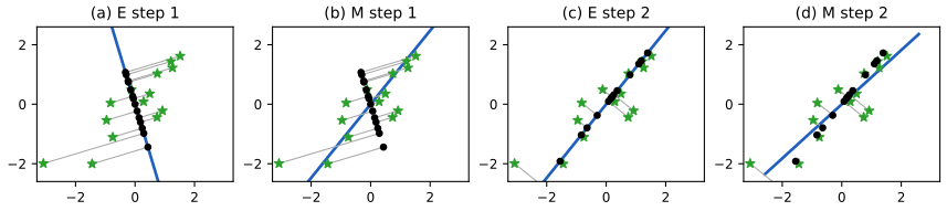
pp. 670–671 In the noise-free limit \(\sigma^2=0\), with \(\tilde{\bm X}=\bm X^\T\) (\(D\times N\)) and \(\tilde{\bm Z}=\bm Z^\T\) (\(L\times N\)), EM reads \[ \tilde{\bm Z}=(\bm W^\T\bm W)^{-1}\bm W^\T\tilde{\bm X}\quad(\text{E step}),\qquad\bm W=\tilde{\bm X}\tilde{\bm Z}^\T(\tilde{\bm Z}\tilde{\bm Z}^\T)^{-1}\quad(\text{M step}) . \tag{20.61–20.64} \] The E step projects the data onto the rod \(\bm W\); the M step is multi-output linear regression (11.2) of the data on the latent values. The mechanical analogy (Roweis, 1997): points attached by springs to a rigid rod; the E step slides the attachments to minimise the spring energy, the M step rotates the rod (Figure 20.10). Advantages: cost \(O(TLND)\) with a small iteration count \(T\), online and missing-data versions, and extensions (mixtures, variational forms). Tipping and Bishop (1999) showed that the only stable fixed point is the global optimum, so \(\bm W\) converges to a basis of the principal subspace (not necessarily orthonormal, and not ordered by eigenvalue; one orthogonalises afterwards).
Filling the gap 20.9: EM for PCA is subspace iteration, with rate \(\lambda_{L+1}/\lambda_L\) pp. 670–671, (20.61)–(20.64)
Proof
The update in closed form. Let \(\bm A=\tilde{\bm X}\tilde{\bm X}^\T=N\bm S\) (\(D\times D\)). From (20.61), \(\tilde{\bm X}\tilde{\bm Z}^\T=\bm A\bm W(\bm W^\T\bm W)^{-1}\) and \(\tilde{\bm Z}\tilde{\bm Z}^\T=(\bm W^\T\bm W)^{-1}\bm W^\T\bm A\bm W(\bm W^\T\bm W)^{-1}\). Therefore \[ \bm W_{\rm new}=\bm A\bm W(\bm W^\T\bm W)^{-1}\Big[(\bm W^\T\bm W)^{-1}\bm W^\T\bm A\bm W(\bm W^\T\bm W)^{-1}\Big]^{-1}=\bm A\bm W\,(\bm W^\T\bm A\bm W)^{-1}\bm W^\T\bm W . \] So \(\bm W_{\rm new}=(\bm A\bm W)\bm T\) with the \(L\times L\) matrix \(\bm T=(\bm W^\T\bm A\bm W)^{-1}\bm W^\T\bm W\), invertible whenever \(\bm W\) has full column rank and \(\bm A\) is positive definite on its range. Hence \[ \mathrm{span}(\bm W_{t+1})=\mathrm{span}(\bm S\bm W_t) , \] which is one step of subspace (orthogonal) iteration for \(\bm S\), generalising the power method. A numerical experiment on a \(D=8\), \(L=2\) problem confirms that the span of the EM update equals the span of \(\bm S\bm W\) to a principal angle below \(10^{-6}\) at every step (the floor is the accuracy of the arccosine).
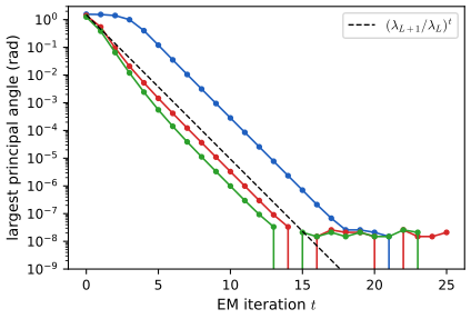
Convergence. Let \(\lambda_L>\lambda_{L+1}\) and write \(\bm W_0=\bm U_L\bm A_1+\bm U_\perp\bm A_2\) with \(\bm U_\perp\) the remaining eigenvectors; assume \(\bm A_1\) invertible (true for almost every starting \(\bm W_0\)). Then \(\bm S^t\bm W_0=\bm U_L\bm\Lambda_L^t\bm A_1+\bm U_\perp\bm\Lambda_\perp^t\bm A_2\). A subspace with basis \(\bm U_L\bm B_1+\bm U_\perp\bm B_2\) has largest principal-angle tangent \(\|\bm B_2\bm B_1^{-1}\|_2\) to \(\mathrm{span}(\bm U_L)\), so \[ \tan\theta_t=\|\bm\Lambda_\perp^t\bm A_2\bm A_1^{-1}\bm\Lambda_L^{-t}\|_2\le\Big(\frac{\lambda_{L+1}}{\lambda_L}\Big)^t\tan\theta_0 . \] Thus the principal subspace is globally attracting from generic starts and the angle shrinks geometrically by \(\lambda_{L+1}/\lambda_L\) per sweep: the number of sweeps is independent of \(N\) and \(D\) and depends only on the eigengap, matching Roweis's observation that very few iterations are needed (3.6 on average in his experiments) when the eigenvalues are well separated. Every other fixed subspace (spanned by a different set of eigenvectors) is unstable: a small component along a more dominant direction is amplified by the ratio of the eigenvalues, which is Tipping and Bishop's stability statement. Figure 20.S1: three random starts for a ten-dimensional problem with \(\lambda_3/\lambda_2=0.30\); each curve decays at (or faster than) the dashed line \((\lambda_3/\lambda_2)^t\) until it reaches the numerical floor. The demonstration above shows the same factor in two dimensions (preset 2: \(\lambda_2/\lambda_1=0.8\) is slow).
With noise. For \(\sigma^2>0\) the EM updates are \(\bm W_{\rm new}=\bm S\bm W(\sigma^2\bm I+\bm M^{-1}\bm W^\T\bm S\bm W)^{-1}\), \(\sigma^2_{\rm new}=\frac1D\Tr(\bm S-\bm S\bm W\bm M^{-1}\bm W_{\rm new}^\T)\) with \(\bm M=\bm W^\T\bm W+\sigma^2\bm I\) (Tipping and Bishop, 1999). They again keep the span in \(\mathrm{span}(\bm S\bm W)\), increase the likelihood at every step, and converge to the maximum of Gap 20.7 (checked numerically: monotone, final \(\sigma^2\) equal to the mean of the discarded eigenvalues to \(10^{-4}\)). The rod demonstration with "EM for PPCA" shows the shrinking of \(\|\bm w\|^2\) to \(\lambda_1-\sigma^2\). \(\square\)
20.2.3.3 Advantages
p. 671 EM can be faster than eigen-solvers when \(N,D\gg L\) (the cost of each sweep is dominated by the projections, \(O(LND)\)), can run online, handles missing data (the E step uses only observed coordinates) and extends to mixtures and to variational Bayes. Sophisticated eigen-solvers such as Lanczos have comparable cost.
20.2.4 Unidentifiability of the parameters
pp. 671–673 The covariance \(\bm W\bm W^\T+\bm\Psi\) is unchanged by \(\bm W\mapsto\bm W\bm R\) with \(\bm R\bm R^\T=\bm I\) (20.65, 20.66): the isotropic latent prior is rotation invariant, so the loadings, and the factors, are identifiable only up to a rotation. Remedies the book lists: (1) orthonormal columns, the PCA choice (unique up to the order of the dimensions, resolved by sorting by eigenvalue); (2) a lower-triangular \(\bm W\) with positive diagonal (20.67), popular in Bayesian treatments, with \(D+DL-L(L-1)/2\) free parameters, the number of identifiable parameters of FA; its drawback is that the first \(L\) variables (the "founders") shape the factors; (3) sparsity-promoting priors on \(\bm W\) (\(\ell_1\), ARD, spike-and-slab: sparse FA); (4) heuristic rotations such as varimax (Kaiser, 1958), which push the loadings towards sparsity; (5) non-Gaussian priors on \(\bm z\), which can make \(\bm W\) and the factors identifiable (the setting of independent component analysis).
Filling the gap 20.10: the parameter count of factor analysis and the lower-triangular normal form pp. 672–673, footnote 3, (20.65)–(20.67)
Derivation
Rotations are the only ambiguity in \(\bm W\bm W^\T\). If \(\bm W_1\bm W_1^\T=\bm W_2\bm W_2^\T\) with \(\bm W_i\in\R^{D\times L}\) of full column rank, then \(\bm W_2=\bm W_1\bm R\) with \(\bm R=\bm W_1^+\bm W_2\) orthogonal: the two matrices have the same column space (the range of the common Gram matrix), \(\bm W_1^\T\bm W_1\) and \(\bm W_2^\T\bm W_2\) are conjugate, and \(\bm R\bm R^\T=\bm W_1^+\bm W_2\bm W_2^\T\bm W_1^{+\T}=\bm W_1^+\bm W_1\bm W_1^\T\bm W_1^{+\T}=\bm I\). The orthogonal group \(O(L)\) has dimension \(L(L-1)/2\) (the book's column-by-column count: \(L-1\) free numbers in the first unit column, \(L-2\) in the next, and so on). Hence the covariance family \(\{\bm W\bm W^\T+\bm\Psi\}\) has \(DL-L(L-1)/2+D\) parameters locally, generically. This was confirmed numerically: for \(D=6\), \(L=2\), the Jacobian of \((\bm W,\bm\Psi)\mapsto\mathrm{vec}(\bm W\bm W^\T+\bm\Psi)\) has rank 17 \(=6+12-1\).
Lower-triangular normal form. Partition \(\bm W=\begin{pmatrix}\bm W_1\\\bm W_2\end{pmatrix}\) with \(\bm W_1\in\R^{L\times L}\) invertible, and let \(\bm K=\bm W\bm W^\T\). Then \(\bm K_{11}=\bm W_1\bm W_1^\T\) and \(\bm K_{21}=\bm W_2\bm W_1^\T\). The Cholesky factor of \(\bm K_{11}\) is the unique lower-triangular matrix with positive diagonal \(\bm W_1\) with this product; then \(\bm W_2=\bm K_{21}\bm W_1^{-\T}\). So requiring \(\bm W_1\) lower triangular with \(w_{kk}>0\) picks exactly one \(\bm W\) from each rotation orbit (when the top \(L\times L\) block is invertible), with \(L(L+1)/2+(D-L)L=DL-L(L-1)/2\) free entries, as in (20.67).
When is the model identifiable at all? A covariance \(\bm C\) has \(D(D+1)/2\) free entries, so FA can be injective on the parameter space only if \(D(D+1)/2\ge D+DL-L(L-1)/2\), i.e. \((D-L)^2\ge D+L\) (Ledermann's bound, 1937). For \(D=4\) this allows only \(L=1\); with \(D=6\), \(L\le3\). Beyond the bound a covariance can be fitted exactly with many different \((\bm W,\bm\Psi)\) and the likelihood cannot discriminate. \(\square\)
20.2.5 Nonlinear factor analysis
pp. 673–674 Replace \(\bm W\bm z\) by a neural network: \(p(\bm x)=\int\N(\bm x\given f(\bm z;\bm\theta),\bm\Psi)\N(\bm z\given\bm 0,\bm I)\,\d\bm z\) (20.68). Neither the posterior nor the marginal likelihood is available in closed form; the variational autoencoder of Section 20.3.5 is the standard approximation.
20.2.6 Mixtures of factor analyzers
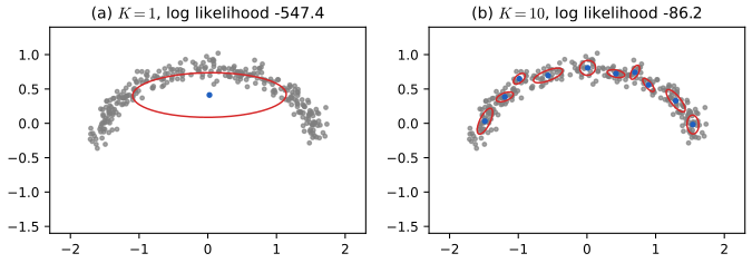
p. 674 A mixture of FA models is locally linear: with component indicator \(m_n\sim\mathrm{Cat}(\bm\pi)\), \[ p(\bm x_n\given\bm z_n,m_n=k)=\N(\bm x_n\given\bm\mu_k+\bm W_k\bm z_n,\bm\Psi_k),\quad p(\bm z_n)=\N(\bm 0,\bm I),\quad p(m_n=k)=\pi_k , \tag{20.69–20.71} \] so that \(p(\bm x)=\sum_k\pi_k\N(\bm x\given\bm\mu_k,\bm W_k\bm W_k^\T+\bm\Psi_k)\): a mixture of Gaussians with low-rank-plus-diagonal covariances, using \(O(KLD)\) parameters against \(O(KD^2)\). With \(\bm\Psi_k=\sigma^2\bm I\) it is a mixture of PPCA models (the orthogonality of the \(\bm W_k\) is then not guaranteed). Figure 20.12 fits a mixture of PPCA models with \(L=1\) to a curved cloud: one component gives a straight ellipse, ten components follow the curve.
Filling the gap 20.11: EM for a mixture of factor analysers and of PPCA models pp. 674–675, (20.69)–(20.72), Exercise 20.2
Derivation
The model as printed. Equation (20.72) writes \(p(\bm x)=\sum_kp(c=k)\int\N(\bm z\given\bm\mu_k,\bm I)\N(\bm x\given\bm W\bm z,\sigma^2\bm I)\,\d\bm z\), which does not match (20.69)–(20.71): the prior of \(\bm z\) has mean \(\bm 0\), the mean \(\bm\mu_k\) belongs to the likelihood, the matrix is \(\bm W_k\), and the noise is \(\bm\Psi_k\). The correct marginal follows from Gap 20.6 for each component: \(\sum_k\pi_k\N(\bm x\given\bm\mu_k,\bm W_k\bm W_k^\T+\bm\Psi_k)\).
E step. The latent variables are \((m_n,\bm z_n)\). The responsibility is \(r_{nk}=p(m_n=k\given\bm x_n)=\pi_k\N(\bm x_n\given\bm\mu_k,\bm C_k)/\sum_j\pi_j\N(\bm x_n\given\bm\mu_j,\bm C_j)\) with \(\bm C_k=\bm W_k\bm W_k^\T+\bm\Psi_k\); given \(m_n=k\), \(p(\bm z_n\given\bm x_n,m_n=k)=\N(\bm m_{nk},\bm\Sigma_k)\) with \(\bm\Sigma_k=(\bm I+\bm W_k^\T\bm\Psi_k^{-1}\bm W_k)^{-1}\), \(\bm m_{nk}=\bm\Sigma_k\bm W_k^\T\bm\Psi_k^{-1}(\bm x_n-\bm\mu_k)\) (Gap 20.6). M step. The expected complete-data log likelihood is \(Q=\sum_n\sum_kr_{nk}\{\log\pi_k+\E_{\bm z\sim p(\cdot\mid\bm x_n,k)}[\log\N(\bm x_n\given\tilde{\bm W}_k\tilde{\bm z},\bm\Psi_k)+\log\N(\bm z\given\bm 0,\bm I)]\}\). It splits: \(\pi_k=\frac1N\sum_nr_{nk}\) (Lagrange multiplier for \(\sum\pi_k=1\)), and for each \(k\) the terms in \((\tilde{\bm W}_k,\bm\Psi_k)\) are those of Gap 20.8 with every datum weighted by \(r_{nk}\): \[ \tilde{\bm W}_k=\Big[\sum_nr_{nk}\bm x_n\bm b_{nk}^\T\Big]\Big[\sum_nr_{nk}\bm C_{nk}\Big]^{-1},\qquad\bm\Psi_k=\frac{\diag\{\sum_nr_{nk}(\bm x_n-\tilde{\bm W}_k\bm b_{nk})\bm x_n^\T\}}{\sum_nr_{nk}} , \] with \(\bm b_{nk}=(\bm m_{nk};1)\) and \(\bm C_{nk}\) as in (20.58) (Exercise 20.2).
A variant for PPCA components. If instead only the indicator \(m_n\) is treated as missing, the M step for \((\bm\mu_k,\bm W_k,\sigma_k^2)\) maximises \(\sum_nr_{nk}\log\N(\bm x_n\given\bm\mu_k,\bm W_k\bm W_k^\T+\sigma_k^2\bm I)\), a weighted PPCA likelihood whose global maximum is Gap 20.7 applied to the weighted covariance \(\bm S_k=\sum_nr_{nk}(\bm x_n-\bm\mu_k)(\bm x_n-\bm\mu_k)^\T/\sum_nr_{nk}\) with \(\bm\mu_k\) the weighted mean. This is a valid EM step (the bound built from \(r_{nk}\) alone is tight at the current parameters and is maximised exactly), and it is what the code uses: the log likelihood is non-decreasing across iterations, and with \(K=1\) it returns the single-PPCA maximum. \(\square\)
20.2.7 Exponential family factor analysis
pp. 675–677 For non-real data replace the Gaussian output by an exponential-family distribution whose natural parameters are a low-rank function of the latent variables, \(\bm\Theta=\bm Z\bm W\) (\(N\times D\) matrix of natural parameters, \(\bm Z\in\R^{N\times L}\), \(\bm W\in\R^{L\times D}\)) (20.73). There is no conjugacy, so neither the posterior nor the marginal likelihood is available. Alternating point estimates of \(\bm z_n\) and \(\bm W\) is exponential family PCA (Collins et al., 2002), a degenerate (delta-posterior) variational EM that overfits because the number of latent variables grows with \(N\); a Gaussian variational posterior fixes this. Two examples: binary PCA, \(p(\bm x\given\bm z)=\prod_d\mathrm{Ber}(x_d\given\sigma(\bm w_d^\T\bm z))\) (20.74), and categorical PCA, \(p(\bm x\given\bm z)=\prod_d\mathrm{Cat}(x_d\given\mathrm{softmax}(\bm W_d\bm z))\) (20.76).
20.2.7.1 Example: binary PCA
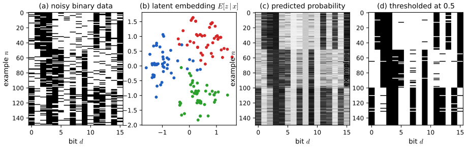
pp. 675–676 The book draws 150 bit vectors of length 16, each a noisy copy of one of three binary prototypes, and fits \(L=2\) by variational EM (Tipping, 1998). Figure 20.13(b) shows the embeddings \(\E[\bm z_n\given\bm x_n]\), (c) the posterior predictive probabilities of each bit (20.75) and (d) their thresholded version, a denoised data set.
Filling the gap 20.12: the Jaakkola–Jordan bound and variational EM for binary PCA pp. 675–676, (20.74), (20.75); Tipping (1998)
Derivation
The bound. For \(a\in\R\), \(\log\sigma(a)=\frac a2-\log(2\cosh\frac a2)=\frac a2-\psi(a^2)\) with \(\psi(x)=\log2\cosh(\sqrt x/2)\). The function \(\psi\) is concave in \(x\ge0\): \(\psi'(x)=\frac{\tanh(\sqrt x/2)}{4\sqrt x}=\frac18\,\frac{\tanh s}{s}\) with \(s=\sqrt x/2\), and \(\tanh s/s\) is decreasing for \(s>0\) (its derivative has the sign of \(s\,\mathrm{sech}^2s-\tanh s\), which is \(\le0\) because it is equivalent to \(\sinh s\cosh s\ge s\)), so \(\psi'\) is decreasing. A concave function lies below its tangents: \(\psi(a^2)\le\psi(\xi^2)+\psi'(\xi^2)(a^2-\xi^2)\). Hence, with \(\lambda(\xi)=\psi'(\xi^2)=\frac{\tanh(\xi/2)}{4\xi}=\frac{\sigma(\xi)-\frac12}{2\xi}\) (since \(\tanh\frac\xi2=2\sigma(\xi)-1\)), \[ \log\sigma(a)\ \ge\ \log\sigma(\xi)+\frac{a-\xi}{2}-\lambda(\xi)\,(a^2-\xi^2),\qquad\text{with equality at }a=\pm\xi . \] For a bit \(x\in\{0,1\}\) and \(t=2x-1\), \(\log p(x\given a)=\log\sigma(ta)\), and as \(\lambda\) is even the bound reads \(\log\sigma(\xi)+\frac{ta-\xi}2-\lambda(\xi)(a^2-\xi^2)\).
Variational EM. Let \(a_{nd}=\bm w_d^\T\bm z_n+b_d\) and give every entry its own parameter \(\xi_{nd}\). Replacing each likelihood factor by its bound gives a function \(B(\bm\theta,\bm\xi,q)\) that lower-bounds \(\log p(\bm X\given\bm\theta)\) once \(q\) is a posterior approximation. E step: the optimal \(q(\bm z_n)\) is proportional to \(p(\bm z_n)\exp\{\sum_d[(x_{nd}-\frac12)a_{nd}-\lambda_{nd}a_{nd}^2]\}\), a Gaussian \(\N(\bm m_n,\bm S_n)\) with \(\bm S_n^{-1}=\bm I+2\sum_d\lambda_{nd}\bm w_d\bm w_d^\T\) and \(\bm m_n=\bm S_n\sum_d[(x_{nd}-\frac12)-2\lambda_{nd}b_d]\bm w_d\). M step: with \(\tilde{\bm w}_d=(\bm w_d,b_d)\), \(\tilde{\bm z}=(\bm z,1)\), the terms in \(\tilde{\bm w}_d\) are \(\sum_n\E[(x_{nd}-\frac12)\tilde{\bm w}_d^\T\tilde{\bm z}_n-\lambda_{nd}(\tilde{\bm w}_d^\T\tilde{\bm z}_n)^2]\); setting the gradient to zero, \(\tilde{\bm w}_d=\big(2\sum_n\lambda_{nd}\E[\tilde{\bm z}_n\tilde{\bm z}_n^\T]\big)^{-1}\sum_n(x_{nd}-\frac12)\E[\tilde{\bm z}_n]\). Variational parameters: the bound is tightest when \(\xi_{nd}^2=\E[a_{nd}^2]=\tilde{\bm w}_d^\T\E[\tilde{\bm z}_n\tilde{\bm z}_n^\T]\tilde{\bm w}_d\) (the bound's dependence on \(\xi\) is through \(\log\sigma(\xi)-\frac\xi2+\lambda\xi^2\), whose stationarity in \(\xi\) gives this). Each of the three updates cannot decrease the bound \(B\), which is checked numerically to be non-decreasing over 60 iterations and never above the exact log likelihood (the latter computed by two-dimensional quadrature over \(\bm z\)).
Prediction. (20.75) integrates \(\sigma(\bm w_d^\T\bm z+b_d)\) over the Gaussian posterior; the probit approximation \(\sigma(\mu_a/\sqrt{1+\pi v_a/8})\) with \(\mu_a=\bm w_d^\T\bm m_n+b_d\), \(v_a=\bm w_d^\T\bm S_n\bm w_d\) (Section 10.5.2) gives the probabilities of Figure 20.13(c). \(\square\)
20.2.7.2 Example: categorical PCA
p. 677 The same construction with a categorical likelihood (20.76) is categorical PCA; a variational EM algorithm is given by Khan et al. (2010).
20.2.8 Factor analysis models for paired data
pp. 677–679 With two kinds of observation, \(\bm x\in\R^{D_x}\) and \(\bm y\in\R^{D_y}\) (two sensors, or inputs and targets), share some latent factors. Supervised PCA (Yu et al., 2006): \(\bm z\sim\N(\bm 0,\bm I_L)\), \(\bm x\sim\N(\bm W_x\bm z,\sigma_x^2\bm I)\), \(\bm y\sim\N(\bm W_y\bm z,\sigma_y^2\bm I)\) (20.77–20.79); for a scalar \(y\), integrating out \(\bm z\) gives \[ p(y\given\bm x)=\N\big(y\given\bm x^\T\bm v,\ \bm w_y^\T\bm C\bm w_y+\sigma_y^2\big),\quad\bm C=(\bm I+\sigma_x^{-2}\bm W_x^\T\bm W_x)^{-1},\quad\bm v=\sigma_x^{-2}\bm W_x\bm C\bm w_y . \tag{20.80–20.82} \] To emphasise prediction, weight the \(\bm x\)-likelihood by \(\alpha\le1\) (20.83). Partial least squares adds a private latent variable \(\bm z^x\) for \(\bm x\) alone (20.84–20.86): \(\bm x\sim\N(\bm W_x\bm z^s+\bm B_x\bm z^x,\sigma_x^2\bm I)\), \(\bm y\sim\N(\bm W_y\bm z^s,\sigma_y^2\bm I)\). Canonical correlation analysis adds a private variable for each side (20.87–20.90); marginalising all latents gives a Gaussian on \((\bm x,\bm y)\) with a low-rank covariance (20.91, 20.92), and Bach and Jordan (2005) showed that its maximum likelihood estimate is classical CCA (Hotelling, 1936).
Filling the gap 20.13: the predictive distribution of supervised PCA, and CCA as a singular value problem pp. 677–679, (20.80)–(20.92)
Derivation
Supervised PCA, (20.80)–(20.82). Given \(\bm x\), the posterior of \(\bm z\) is that of Gap 20.6 with \(\bm W=\bm W_x\), \(\bm\Psi=\sigma_x^2\bm I\): \(\bm z\given\bm x\sim\N(\sigma_x^{-2}\bm C\bm W_x^\T\bm x,\bm C)\) with \(\bm C=(\bm I+\sigma_x^{-2}\bm W_x^\T\bm W_x)^{-1}\) (20.81). Since \(y=\bm w_y^\T\bm z+\epsilon_y\) with \(\epsilon_y\sim\N(0,\sigma_y^2)\) independent of \(\bm x\) given \(\bm z\), \(y\given\bm x\) is Gaussian with mean \(\bm w_y^\T\sigma_x^{-2}\bm C\bm W_x^\T\bm x=\bm x^\T\bm v\), \(\bm v=\sigma_x^{-2}\bm W_x\bm C\bm w_y\) (using \(\bm C^\T=\bm C\)) (20.82), and variance \(\bm w_y^\T\bm C\bm w_y+\sigma_y^2\) (20.80). This agrees numerically with Gaussian conditioning of the joint Gaussian \((\bm x,y)\), whose covariance blocks are \(\bm W_x\bm W_x^\T+\sigma_x^2\bm I\), \(\bm W_x\bm w_y\) and \(\bm w_y^\T\bm w_y+\sigma_y^2\). The model is symmetric in \(\bm x\) and \(\bm y\); weighting \(\log p(\bm x\given\bm z)\) by \(\alpha<1\) (20.83) lets the fit concentrate on the part of \(\bm x\) that predicts \(\bm y\).
Classical CCA. For random vectors with covariances \(\bm\Sigma_{xx},\bm\Sigma_{yy}\) (positive definite) and cross-covariance \(\bm\Sigma_{xy}\), CCA seeks \(\bm a,\bm b\) maximising \(\rho=\frac{\bm a^\T\bm\Sigma_{xy}\bm b}{\sqrt{\bm a^\T\bm\Sigma_{xx}\bm a}\sqrt{\bm b^\T\bm\Sigma_{yy}\bm b}}\). Substitute \(\bm a'=\bm\Sigma_{xx}^{1/2}\bm a\), \(\bm b'=\bm\Sigma_{yy}^{1/2}\bm b\) and \(\bm K=\bm\Sigma_{xx}^{-1/2}\bm\Sigma_{xy}\bm\Sigma_{yy}^{-1/2}\): \(\rho=\frac{\bm a'^\T\bm K\bm b'}{\|\bm a'\|\|\bm b'\|}\), whose maximum over directions is the largest singular value \(s_1\) of \(\bm K\), attained at the top singular vectors \(\bm u_1,\bm v_1\) (Section 7.5); the next pair \(\bm a_2,\bm b_2\) uncorrelated with the first gives \(s_2\), and so on: \(\bm a_k=\bm\Sigma_{xx}^{-1/2}\bm u_k\), \(\bm b_k=\bm\Sigma_{yy}^{-1/2}\bm v_k\), canonical correlations \(\rho_k=s_k\in[0,1]\). The numerical experiment on simulated paired data (5000 samples, 2 shared factors) shows that the correlation of the projections on the first pair equals \(s_1\) and agrees with scikit-learn's CCA.
The probabilistic model. The covariance (20.92) has blocks \(\bm W_x\bm W_x^\T+\bm B_x\bm B_x^\T+\sigma^2\bm I\) and \(\bm W_x\bm W_y^\T\) off the diagonal: the cross-covariance has rank at most \(L_s\), and the private parts make the diagonal blocks arbitrary positive definite matrices in the limit of full private factors. Maximising the Gaussian likelihood with a free \(\bm\Sigma_{xx},\bm\Sigma_{yy}\) and a rank-\(L_s\) \(\bm\Sigma_{xy}\) is a reduced-rank problem whose solution, by Bach and Jordan (2005), is \(\hat{\bm\Sigma}_{xy}=\hat{\bm\Sigma}_{xx}\bm U_{L_s}\bm M_x\bm M_y^\T\bm V_{L_s}^\T\hat{\bm\Sigma}_{yy}\) built from the leading \(L_s\) canonical directions with \(\bm M_x\bm M_y^\T=\diag(\rho_1,\dots,\rho_{L_s})\); the argument is that the concentrated log likelihood depends on \(\bm\Sigma_{xy}\) only through \(\sum_k\log(1-\rho_k^2)\)-type terms, which are decreasing in each retained canonical correlation. We cite the result and do not reprove it. \(\square\)
20.3 Autoencoders
pp. 679–689 PCA and FA learn a linear encoder \(f_e:\bm x\mapsto\bm z\) and a linear decoder \(f_d:\bm z\mapsto\bm x\), with reconstruction \(r(\bm x)=f_d(f_e(\bm x))\) trained to minimise \(\|r(\bm x)-\bm x\|_2^2\) (more generally \(-\log p(\bm x\given r(\bm x))\)). An autoencoder (AE) lets both maps be neural networks (Figure 20.16, a diagram). If the hidden layer is wide enough the network can learn the identity, so the representation must be constrained: a narrow bottleneck (\(L\ll D\), the undercomplete case) or an overcomplete code (\(L\gg D\)) with a regulariser (input noise, sparsity of the activations, a penalty on the derivatives).
See also: Foundations of Deep Learning, Chapter 19 on autoencoders (deterministic, sparse, denoising and variational autoencoders); Bayesian and Probabilistic ML, Section 12.4.2; the VAE latent explorer.
20.3.1 Bottleneck autoencoders
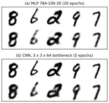
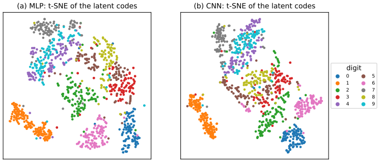
p. 680 The linear autoencoder has one hidden layer, \(\bm z=\bm W_1\bm x\) and \(\hat{\bm x}=\bm W_2\bm z\) with \(\bm W_1\in\R^{L\times D}\), \(\bm W_2\in\R^{D\times L}\), so \(\hat{\bm x}=\bm W_2\bm W_1\bm x\), trained on \(\sum_n\|\bm x_n-\bm W_2\bm W_1\bm x_n\|^2\). The book cites Baldi and Hornik (1989) and Karhunen and Joutsensalo (1995) for the fact that the optimal \(\bm W_2\bm W_1\) is the orthogonal projection onto the top-\(L\) eigenvectors of the covariance, so that this is PCA; adding nonlinearities gives a strictly more powerful model (Japkowicz et al., 2000). The experiment: an MLP encoder 784–100–30 (with the decoder its mirror image) and a CNN autoencoder, both trained with a Bernoulli likelihood (binary cross-entropy) on image data; the CNN reconstructs more accurately (Figure 20.17), and a t-SNE plot of the codes (Figure 20.18) separates the classes without having used labels.
Filling the gap 20.14: a linear autoencoder spans the principal subspace p. 680, Baldi and Hornik (1989)
Proof
Stack the centred data in \(\bm X\in\R^{N\times D}\) with thin SVD \(\bm X=\bm U_X\bm S_X\bm V_X^\T\), singular values \(s_1\ge\dots\ge s_D\). With \(\bm B=(\bm W_2\bm W_1)^\T\) the loss is \(\|\bm X-\bm X\bm B\|_F^2\), and \(\mathrm{rank}\,\bm B\le L\). Lower bound. \(\bm X\bm B\) has rank at most \(L\), so by the Eckart–Young–Mirsky theorem (Result 7.5) \(\|\bm X-\bm X\bm B\|_F^2\ge\sum_{j>L}s_j^2\). Attained. With \(\bm B=\bm V_L\bm V_L^\T\), \(\bm X\bm B=\bm U_L\bm S_L\bm V_L^\T\), the truncated SVD, so the bound is attained, and the minimum equals \(N\sum_{j>L}\lambda_j\), the PCA error of (20.26). All minimisers. If \(s_L>s_{L+1}\), the best rank-\(L\) approximation of \(\bm X\) is unique, so any minimiser has \(\bm X\bm B=\bm U_L\bm S_L\bm V_L^\T\), i.e. \(\bm X(\bm B-\bm V_L\bm V_L^\T)=\bm 0\); if \(\bm X\) has full column rank this gives \(\bm B=\bm V_L\bm V_L^\T\), the orthogonal projector onto the principal subspace. Hence \(\bm W_2\bm W_1=\bm P_L=\bm U_L\bm U_L^\T\): the product is exactly the projector, but the factors are not individually orthonormal: \(\bm W_2=\bm U_L\bm G^{-1}\), \(\bm W_1=\bm G\bm U_L^\T\) for any invertible \(\bm G\in\R^{L\times L}\). The code \(\bm z=\bm G\bm U_L^\T\bm x\) is therefore an invertible linear transformation of the PCA scores, not the scores themselves (the linear autoencoder has the rotation ambiguity of FA, and more). Baldi and Hornik also show that the loss has no local minima other than these global ones (all other critical points are saddles); this part is quoted, not reproved. A numerical experiment (\(D=5\), \(L=2\), 400 points; L-BFGS from random starts) gives a minimum loss equal to the discarded eigenvalue sum to \(10^{-6}\), and \(\bm W_2\bm W_1\) within \(10^{-4}\) of the projector. Nonlinear case. A network with an activation that is the identity on an interval can represent the linear solution with small weights, so the best nonlinear autoencoder is at least as good as PCA with the same \(L\): on the MNIST sample the 30-unit MLP autoencoder reaches a test error of 0.0138 per pixel against 0.0176 for PCA with 30 components, and the 20-unit autoencoder 0.0118 against 0.0234 for PCA with 20. \(\square\)
20.3.2 Denoising autoencoders
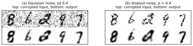
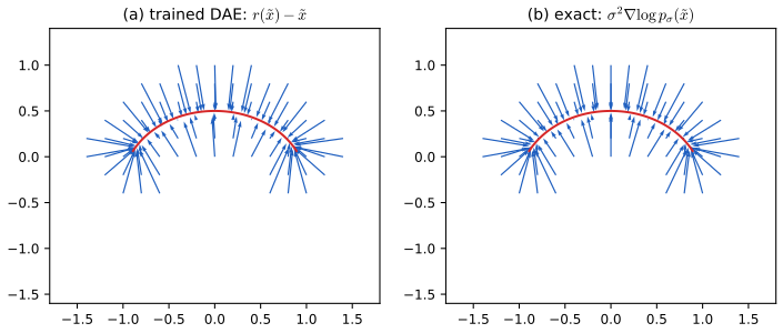
pp. 681–682 A denoising autoencoder (DAE; Vincent et al., 2010) corrupts the input, \(\tilde{\bm x}\sim p_c(\cdot\given\bm x)\) (Gaussian noise or dropout), and is trained to reconstruct the clean \(\bm x\). It can "hallucinate" details missing in the input, because it has stored typical structure in its weights (Figure 20.19). For Gaussian corruption \(p_c(\tilde{\bm x}\given\bm x)=\N(\tilde{\bm x}\given\bm x,\sigma^2\bm I)\) and squared error, Alain and Bengio (2014) show that as \(\sigma\to0\) (with a sufficiently powerful model and enough data) the residual of the DAE approximates the score \(\nabla_{\bm x}\log p(\bm x)\): the DAE learns a vector field pointing to regions of higher density, so points near the data manifold are mapped onto it (Figure 20.20).
Filling the gap 20.15: the DAE residual is \(\sigma^2\) times the score (Tweedie); the contractive penalty pp. 681–683, Figure 20.20, (20.93)
Proof
The optimal denoiser is the posterior mean. The population loss is \(\E\|r(\tilde{\bm x})-\bm x\|^2\) with \(\bm x\sim p\), \(\tilde{\bm x}=\bm x+\sigma\bm\epsilon\). Condition on \(\tilde{\bm x}\): for any function \(r\), \(\E[\|r(\tilde{\bm x})-\bm x\|^2\given\tilde{\bm x}]=\|r(\tilde{\bm x})-\E[\bm x\given\tilde{\bm x}]\|^2+\mathrm{tr}\,\mathrm{cov}[\bm x\given\tilde{\bm x}]\), minimised by \(r^*(\tilde{\bm x})=\E[\bm x\given\tilde{\bm x}]\).
Tweedie's formula (Robbins 1956; Miyasawa 1961). Let \(p_\sigma(\tilde{\bm x})=\int p(\bm x)\N(\tilde{\bm x}\given\bm x,\sigma^2\bm I)\,\d\bm x\) be the density of the corrupted data. Differentiating under the integral, \(\nabla_{\tilde{\bm x}}\N(\tilde{\bm x}\given\bm x,\sigma^2\bm I)=-\frac{\tilde{\bm x}-\bm x}{\sigma^2}\N(\tilde{\bm x}\given\bm x,\sigma^2\bm I)\), so \[ \nabla p_\sigma(\tilde{\bm x})=\frac1{\sigma^2}\Big[-\tilde{\bm x}\,p_\sigma(\tilde{\bm x})+\int\bm x\,p(\bm x)\N(\tilde{\bm x}\given\bm x,\sigma^2\bm I)\,\d\bm x\Big]=\frac{p_\sigma(\tilde{\bm x})}{\sigma^2}\big[\E[\bm x\given\tilde{\bm x}]-\tilde{\bm x}\big] , \] because \(\E[\bm x\given\tilde{\bm x}]=\int\bm x\,p(\bm x)\N(\tilde{\bm x}\given\bm x,\sigma^2\bm I)\,\d\bm x/p_\sigma(\tilde{\bm x})\). Dividing by \(p_\sigma\), \[ r^*(\tilde{\bm x})-\tilde{\bm x}=\sigma^2\nabla_{\tilde{\bm x}}\log p_\sigma(\tilde{\bm x}) . \] As \(\sigma\to0\), \(p_\sigma\to p\) (and \(\nabla\log p_\sigma\to\nabla\log p\) wherever \(p\) is smooth and positive), so the residual of the optimal DAE is \(\sigma^2\) times the score: the book's statement \(\bm e(\bm x)\approx\nabla_{\bm x}\log p(\bm x)\) omits the factor \(\sigma^2\) (and the residual in Alain and Bengio is \(r(\tilde{\bm x})-\tilde{\bm x}\), measured from the corrupted point, whereas the book writes \(r(\tilde{\bm x})-\bm x\) with the clean \(\bm x\)); in Figure 20.20 the arrows are drawn at the scale \(\sigma^2\nabla\log p\), so their lengths are small close to the manifold and larger away from it. I checked Tweedie's identity numerically for a one-dimensional two-component Gaussian mixture, comparing the conditional mean computed by quadrature with \(\tilde x+\sigma^2(\log p_\sigma)'(\tilde x)\), to 6 digits. In Figure 20.20 a small network trained with \(\sigma=0.15\) on a thin arc (a mixture of 80 narrow Gaussians, whose score is known exactly) has a residual field that differs from the exact optimum by 4.8 percent in root mean square relative to the field's own size.
Contractive penalty. For a smooth map \(r\) and small noise, \(r(\bm x+\sigma\bm\epsilon)=r(\bm x)+\sigma\bm J\bm\epsilon+O(\sigma^2)\) with \(\bm J=\partial r/\partial\bm x\). Hence \(\E\|r(\bm x+\sigma\bm\epsilon)-\bm x\|^2=\|r(\bm x)-\bm x\|^2+2\sigma(r(\bm x)-\bm x)^\T\bm J\,\E\bm\epsilon+\sigma^2\E\|\bm J\bm\epsilon\|^2+O(\sigma^3)=\|r(\bm x)-\bm x\|^2+\sigma^2\|\bm J\|_F^2+O(\sigma^3)\), since \(\E\bm\epsilon=\bm 0\) and \(\E\|\bm J\bm\epsilon\|^2=\Tr(\bm J^\T\bm J)\). Thus a DAE with small Gaussian noise is, to first order, a plain autoencoder with a penalty \(\sigma^2\|\bm J\|_F^2\) on the Jacobian of the whole reconstruction (Bishop's equivalence of training with noise and Tikhonov regularisation); the contractive autoencoder (Rifai et al., 2011) of (20.93) penalises \(\lambda\|\partial f_e/\partial\bm x\|_F^2\) of the encoder alone. For sigmoid hidden units \(h_k=\sigma(\bm w_k^\T\bm x+b_k)\) the penalty is cheap: \(\|\partial\bm h/\partial\bm x\|_F^2=\sum_k[h_k(1-h_k)]^2\|\bm w_k\|^2\). A penalty that only constrains the encoder can be cheated by scaling the encoder down by \(\epsilon\) and the decoder up by \(1/\epsilon\) (the penalty goes to 0 with no loss of fit); tying the decoder weights to the transposed encoder weights (with separate biases) rules this out, as the book says. Numerically, for \(r=\tanh(\bm A\bm x+\bm b)\) and \(\sigma=2\times10^{-3}\), the mean of \(\|r(\bm x+\sigma\bm\epsilon)-r(\bm x)\|^2\) over \(4\times10^5\) draws equals \(\sigma^2\|\bm J\|_F^2\) to within 1 percent. \(\square\)
20.3.3 Contractive autoencoders
pp. 682–683 A contractive autoencoder (CAE) adds the penalty \(\Omega(\bm z,\bm x)=\lambda\|\partial f_e(\bm x)/\partial\bm x\|_F^2=\lambda\sum_k\|\nabla_{\bm x}h_k(\bm x)\|^2\) (20.93) to the reconstruction loss. Near a data manifold approximated by locally linear patches, the Jacobian of the encoder gives the local linear approximation; making it contractive pushes off-manifold inputs back towards the manifold. The two terms conflict: a constant encoder minimises the penalty but ignores the input, so only a few units can respond, and only to the most significant variations in the data. The degenerate rescaling solution and the cost of computing the Jacobian are discussed in Gap 20.15.
20.3.4 Sparse autoencoders
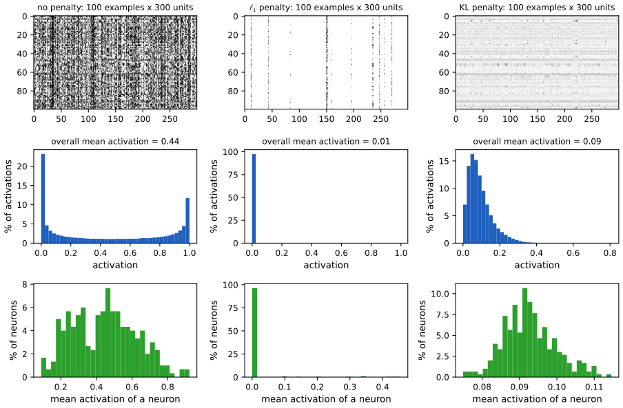
p. 683 Another regulariser is a sparsity penalty on the latent activations, \(\Omega(\bm z)=\lambda\|\bm z\|_1\) (activity regularisation), or, usually better, a KL penalty on the fraction of the time each unit is on. With logistic units, let \(q_k\) be the mean activation of unit \(k\) over a minibatch and \(p\) a target; the penalty is \(\lambda\sum_k\KL(\mathrm{Ber}(p)\,\|\,\mathrm{Ber}(q_k))\) (the book cites Glorot et al., 2011). Figure 20.21 fits an autoencoder with 300 logistic hidden units: without a penalty the activations average 0.39 and most units are partially active most of the time; with the \(\ell_1\) penalty almost all units are off all the time (mean 0.02, many permanently dead); with the KL penalty about 70 percent of the units are off on average at a given example, yet no unit is permanently off (mean activation 0.1), a sparse firing pattern like that of biological neurons.
Filling the gap 20.16: why the KL sparsity penalty equalises the units while \(\ell_1\) switches them off p. 683
Derivation
For logistic units \(z_{nk}\in(0,1)\) the "fraction of time on" is the mean activation \(q_k=\frac1N\sum_nz_{nk}\) (the book writes it as an average of the indicator \(\mathbb I(z_{nk}=1)\), which is the same quantity for binary units). With \(\mathrm{KL}(p\|q)=p\log\frac pq+(1-p)\log\frac{1-p}{1-q}\), \(\frac{\partial}{\partial q}\mathrm{KL}=\frac{q-p}{q(1-q)}\) and \(\frac{\partial^2}{\partial q^2}\mathrm{KL}=\frac{p}{q^2}+\frac{1-p}{(1-q)^2}>0\): the penalty is strictly convex in \(q_k\), zero exactly at \(q_k=p\), and its gradient with respect to each activation \(z_{nk}\) is \(\frac\lambda N\frac{q_k-p}{q_k(1-q_k)}\), the same for every example: it pushes all the activations of unit \(k\) down when the unit is on more than \(p\) of the time and up when it is on less. A unit that is always off is penalised (it has \(q_k\ll p\) and the gradient pulls it up with strength \(\approx p/q_k\)), so the KL penalty cannot kill units; it controls the average but not the per-example sparsity pattern. The \(\ell_1\) penalty \(\lambda\sum_{n,k}|z_{nk}|\) instead has a constant gradient \(\lambda\,\mathrm{sign}(z_{nk})\) towards zero (like the lasso, Section 11.4) that does not vanish for small activations, so units that are not needed are driven to exactly zero (or to the boundary of the sigmoid). Numbers from Figure 20.21 (test images): mean activation 0.44, 0.011 and 0.093, units with mean below 0.01 of 0, 96 and 0 percent, test reconstruction error 0.0142, 0.0388 and 0.0437 per pixel for no penalty, \(\ell_1\) and KL respectively. \(\square\)
20.3.5 Variational autoencoders
pp. 683–689 The variational autoencoder (VAE; Kingma and Welling, 2014; Rezende et al., 2014) is a probabilistic autoencoder and a generative model. It combines two ideas: a nonlinear factor analysis model, replacing \(p(\bm x\given\bm z)=\N(\bm x\given\bm W\bm z,\sigma^2\bm I)\) by \[ p_\theta(\bm x\given\bm z)=\N\big(\bm x\given f_d(\bm z;\bm\theta),\sigma^2\bm I\big) \tag{20.94} \] (for binary data a Bernoulli likelihood with probabilities \(f_d(\bm z;\bm\theta)\); the book's (20.95) writes "\(\mathrm{Ber}(x_i\given f_d(\bm z;\bm\theta),\sigma^2\bm I)\)", but a Bernoulli has no variance parameter), together with an inference network \(q_\phi(\bm z\given\bm x)=\N\big(\bm z\given f_{e,\mu}(\bm x;\bm\phi),\diag(f_{e,\sigma}(\bm x;\bm\phi))\big)\) (20.96) trained at the same time to approximate the posterior. Using one network to invert another, instead of running an optimiser per data point, is amortized inference (Helmholtz machine, Dayan et al., 1995, which used the wake–sleep algorithm; the VAE has a single objective).
20.3.5.1 Training VAEs
p. 685 Since the marginal likelihood is intractable, maximise the evidence lower bound, for one example \[ \mathcal L(\bm\theta,\bm\phi\given\bm x)=\E_{q_\phi(\bm z\mid\bm x)}\big[\log p_\theta(\bm x,\bm z)-\log q_\phi(\bm z\given\bm x)\big]=\E_{q_\phi}\big[\log p_\theta(\bm x\given\bm z)\big]-\KL\big(q_\phi(\bm z\given\bm x)\,\|\,p(\bm z)\big) , \tag{20.97, 20.98} \] an expected log likelihood plus a regulariser that keeps the posterior close to the prior; by Jensen's inequality \(\mathcal L\le\log p_\theta(\bm x)\) (20.99, 20.100). (The book contrasts this with the KL on the aggregate posterior of the sparse autoencoder of Section 20.3.4.)
20.3.5.2 The reparameterization trick
p. 686 Sampling \(\bm z\sim q_\phi\) is not differentiable in \(\bm\phi\). Write \(\bm z=f_{e,\mu}(\bm x;\bm\phi)+f_{e,\sigma}(\bm x;\bm\phi)\odot\bm\epsilon\) with \(\bm\epsilon\sim\N(\bm 0,\bm I)\) (20.101): then \[ \mathcal L(\bm\theta,\bm\phi\given\bm x)=\E_{\bm\epsilon\sim\N(\bm 0,\bm I)}\big[\log p_\theta(\bm x\given\bm z=\bm\mu_\phi(\bm x)+\bm\sigma_\phi(\bm x)\odot\bm\epsilon)\big]-\KL\big(q_\phi(\bm z\given\bm x)\,\|\,p(\bm z)\big) , \tag{20.102} \] the expectation no longer depends on the parameters of the distribution it is taken with, gradients go inside it, and backpropagation applies (Figure 20.23, a diagram). The first term is estimated by one sample of \(\bm\epsilon\); the second is the KL between Gaussians, in closed form for \(p=\N(\bm 0,\bm I)\): \[ \KL(q\|p)=\sum_{k=1}^K\Big[\log\frac1{\sigma_k}+\frac{\sigma_k^2+\mu_k^2}{2}-\frac12\Big]=-\frac12\sum_{k=1}^K\big[\log\sigma_k^2-\sigma_k^2-\mu_k^2+1\big] \tag{20.103} \] (here \(\sigma_k\) is the standard deviation, so "\(\diag(\bm\sigma)\)" in the book is a covariance with diagonal \(\sigma_k^2\)).
Filling the gap 20.17: the ELBO identities, the reparameterisation gradient, the Gaussian KL, and the linear VAE as PPCA pp. 685–687, (20.97)–(20.103)
Derivation
The gap in the bound. For any \(q(\bm z\given\bm x)\), \(\log p(\bm x)=\E_q\big[\log\frac{p(\bm x,\bm z)}{p(\bm z\given\bm x)}\big]=\E_q\big[\log\frac{p(\bm x,\bm z)}{q(\bm z\given\bm x)}\big]+\E_q\big[\log\frac{q(\bm z\given\bm x)}{p(\bm z\given\bm x)}\big]\), that is \[ \log p_\theta(\bm x)=\mathcal L(\bm\theta,\bm\phi\given\bm x)+\KL\big(q_\phi(\bm z\given\bm x)\,\|\,p_\theta(\bm z\given\bm x)\big)\ \ge\ \mathcal L(\bm\theta,\bm\phi\given\bm x) , \] which gives (20.100) without Jensen and tells how loose the bound is: \(\mathcal L\) is tight exactly when \(q_\phi\) equals the true posterior. For fixed \(\bm\theta\), maximising over \(\bm\phi\) is minimising a KL to the posterior; maximising over \(\bm\theta\) raises the likelihood as in EM (Section 8.7.2, where the E step makes \(q\) exact). The identity holds for the linear Gaussian model of PPCA, where I verified it numerically with an arbitrary Gaussian \(q\) and the exact KL between Gaussians.
The Gaussian KL. In one coordinate, with \(q=\N(\mu,\sigma^2)\) and \(p=\N(0,1)\), \(\E_q[\log q]=-\frac12\log(2\pi\sigma^2)-\frac12\) and \(\E_q[\log p]=-\frac12\log2\pi-\frac12(\sigma^2+\mu^2)\) (since \(\E_qz^2=\sigma^2+\mu^2\)), so \(\KL=-\frac12\log\sigma^2-\frac12+\frac12(\sigma^2+\mu^2)\); summing over coordinates gives (20.103). A Monte Carlo estimate with \(2\times10^6\) draws agrees to three decimals.
The reparameterisation gradient. If \(\bm z=\bm g_\phi(\bm\epsilon)=\bm\mu_\phi+\bm\sigma_\phi\odot\bm\epsilon\) then \(\E_{q_\phi}[h(\bm z)]=\E_{\bm\epsilon}[h(\bm g_\phi(\bm\epsilon))]\) (change of variables), and when \(h\) and \(\bm g_\phi\) are differentiable with an integrable derivative, \(\nabla_\phi\E_{\bm\epsilon}[h(\bm g_\phi(\bm\epsilon))]=\E_{\bm\epsilon}[\nabla_{\bm z}h\,\partial_\phi\bm g_\phi]\) (dominated convergence): the pathwise estimator is unbiased. The score-function estimator \(\E_q[h\,\nabla_\phi\log q_\phi]\) is also unbiased but typically has much larger variance, because it ignores the gradient of \(h\). Check for \(h(z)=z^4\): \(\E[(\mu+\sigma\epsilon)^4]=\mu^4+6\mu^2\sigma^2+3\sigma^4\), so \(\partial_\mu=4\mu^3+12\mu\sigma^2\) and \(\partial_\sigma=12\mu^2\sigma+12\sigma^3\); the averages of \(4z^3\) and \(4z^3\epsilon\) over \(3\times10^6\) draws match both to the Monte Carlo error.
The linear VAE is PPCA. Take \(p(\bm z)=\N(\bm 0,\bm I)\), \(p(\bm x\given\bm z)=\N(\bm W\bm z+\bm\mu,\sigma^2\bm I)\). The exact posterior is Gaussian with covariance \(\sigma^2\bm M^{-1}\) (constant in \(\bm x\)) and mean \(\bm M^{-1}\bm W^\T(\bm x-\bm\mu)\) (linear in \(\bm x\)) (20.52). If the inference network is allowed to be affine in \(\bm x\) with a full constant covariance, it can equal this posterior, the KL gap vanishes, and \(\mathcal L=\log p(\bm x)\) (verified numerically: the ELBO at the exact posterior equals the log density to \(10^{-10}\)). Maximising the ELBO over \((\bm\theta,\bm\phi)\) then maximises the marginal likelihood, whose maximiser is Gap 20.7. So the VAE is a nonlinear PPCA fitted by amortised variational inference; with a diagonal-covariance encoder the linear VAE still finds the principal directions (Lucas et al., 2019), but the rotation inside the subspace is fixed by the diagonal restriction.
VAE against autoencoder. An autoencoder embeds \(\bm x\) at a point; the VAE embeds it in a Gaussian cloud, and the KL term keeps the clouds overlapping and centred on the prior, so the decoder is trained on a neighbourhood of every code, and on most of the region that the prior \(\N(\bm 0,\bm I)\) covers. This is why decoding prior samples gives digits (Figure 20.25a) and the latent space is smoother (Figures 20.26, 20.27). In the experiment below both models have a 20-dimensional code and similar capacity; the reconstructions are equally good (test error 0.0134 for the VAE against 0.0118 for the AE per pixel; PCA with 20 components: 0.0234). \(\square\)
20.3.5.3 Comparison of VAEs and autoencoders
pp. 687–688 The decoder plays the role of the generative model \(p_\theta(\bm x\given\bm z)\) and the encoder that of the inference network \(q_\phi(\bm z\given\bm x)\); reconstruction quality is similar (Figure 20.24). The VAE can generate: sample \(\bm z\sim\N(\bm 0,\bm I)\) and decode to \(\E[\bm x\given\bm z]=f_d(\bm z)\). The AE decoder only ever sees the exact training encodings, so it does not know what to do with random points (Figure 20.25). The latent space of the VAE is also smoother, as the t-SNE of the codes shows (Figure 20.26), and supports latent-space interpolation: for two images \(\bm x_1,\bm x_2\) with codes \(\bm z_i=\E_{q(\bm z\mid\bm x_i)}[\bm z]\), decode \(\bm z=\lambda\bm z_1+(1-\lambda)\bm z_2\), \(0\le\lambda\le1\) (Figure 20.27); the book justifies linear interpolation by the nearly zero curvature of the learned manifold (Shao et al., 2018).
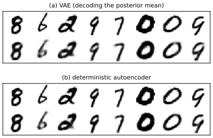
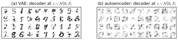
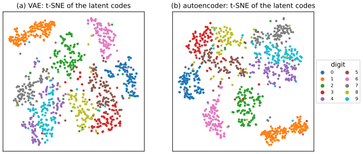
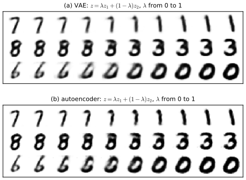
20.4 Manifold learning
pp. 689–705 Manifold learning (nonlinear dimensionality reduction) recovers low-dimensional structure in high-dimensional data, usually assumed to lie near a curved manifold. The methods of this section are nonparametric: they compute an embedding \(\bm z_i\) for each training point but no map that applies to a new point (although Bengio et al., 2004, show how to extend many of them through a kernel). They are used for exploratory visualisation and as preprocessing. See Anowar et al. (2021) for a review.
See also: Bayesian and Probabilistic ML, Section 12.3 (kernel PCA) and its demo; Elements of Statistical Learning, Chapter 14 (multidimensional scaling, local linear embedding and principal curves in Sections 14.8 to 14.9).
20.4.1 What are manifolds?
p. 689 A \(d\)-dimensional manifold is a space in which every point has a neighbourhood topologically equivalent to \(\R^d\) (the surface of the Earth: curved, two-dimensional, locally flat). The Euclidean space that approximates the neighbourhood of \(\bm x\) is the tangent space \(T_{\bm x}\mathcal X\) (Figure 20.28, an illustration). A Riemannian manifold carries an inner product on each tangent space, depending smoothly on the point; it induces lengths, angles and volumes, and distances along the manifold (geodesic distances). Any sufficiently smooth Riemannian manifold can be embedded isometrically in a Euclidean space of possibly higher dimension.
20.4.2 The manifold hypothesis
pp. 689–690 The manifold hypothesis says that naturally occurring high-dimensional data lie close to a low-dimensional manifold. A digit image is a point of \(\R^{3648}\) (Figure 20.29a) but a random binary image is not a digit (b): the pixels are generated by a low-dimensional shape variation. Rotating one image by one degree 360 times gives a closed curve; projected to the first two principal components it is a circle-like loop (c), so the family is parametrised by one angle: its intrinsic dimension is 1, though the ambient dimension is \(784\) here (3648 in the book, which speaks of an underlying curved 2-d manifold: the circle is drawn in a plane but is itself one-dimensional). The first two components keep just 30 percent of the variance; the loop is the projection of a curve that lives in many more dimensions.
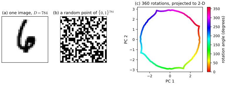
20.4.3 Approaches to manifold learning
pp. 690–691 The methods differ in their assumptions about the manifold and in their computational properties (Table 20.1: whether a parametric map is learned, and whether the problem is convex, and then dense or sparse eigenproblem). The running examples are 1000 points on the Swiss roll (a 2-D manifold in 3-D) and the 1797 UCI digits (64-D, Figure 20.30); the aim is a 2-D embedding.
| Method | Parametric | Convex | Section |
|---|---|---|---|
| PCA / classical MDS | no | yes (dense eigenproblem) | 20.1, 20.4.4 |
| Kernel PCA | no | yes (dense) | 20.4.6 |
| Isomap | no | yes (dense) | 20.4.5 |
| LLE | no | yes (sparse) | 20.4.8 |
| Laplacian eigenmaps | no | yes (sparse) | 20.4.9 |
| t-SNE | no | no | 20.4.10 |
| Autoencoder | yes | no | 20.3 |
Table 20.1 (Murphy, 2022), restated.
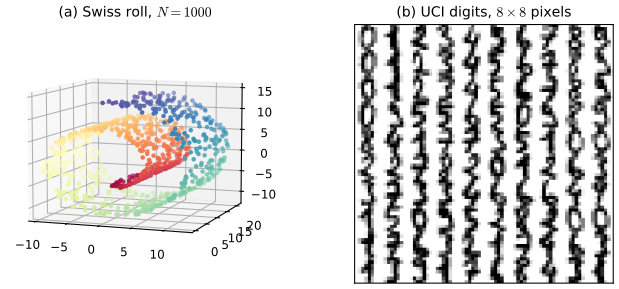
20.4.4 Multi-dimensional scaling (MDS)
pp. 691–694 MDS finds \(\bm z_i\in\R^L\) whose pairwise distances match given dissimilarities \(d_{ij}\). Classical MDS. Let \(\tilde K_{ij}=\langle\bm x_i-\bar{\bm x},\bm x_j-\bar{\bm x}\rangle\), i.e. \(\tilde{\bm K}=\tilde{\bm X}\tilde{\bm X}^\T\) with \(\tilde{\bm X}=\bm C_N\bm X\), \(\bm C_N=\bm I-\frac1N\bm 1\bm 1^\T\) (20.104). The strain of an embedding is \(\mathcal L_{\rm strain}(\bm Z)=\sum_{ij}(\tilde K_{ij}-\langle\tilde{\bm z}_i,\tilde{\bm z}_j\rangle)^2=\|\tilde{\bm K}-\tilde{\bm Z}\tilde{\bm Z}^\T\|_F^2\) (20.105); its minimiser is given by the truncated eigendecomposition, \(\tilde{\bm Z}=\bm U_L\bm S_L^{1/2}\) (20.106). With only distances available, form \(\bm D^{(2)}=\bm D\odot\bm D\) and double-centre: \(\tilde{\bm K}=-\frac12\bm C_N\bm D^{(2)}\bm C_N\) (20.107–20.109). Classical MDS is equivalent to PCA (20.110). Metric MDS allows any dissimilarity and minimises the stress \(\mathcal L_{\rm stress}(\bm Z)=\sqrt{\sum_{i<j}(d_{ij}-\hat d_{ij})^2/\sum_{ij}d_{ij}^2}\), \(\hat d_{ij}=\|\bm z_i-\bm z_j\|\) (20.111), by gradient descent or, better, the bound-optimisation algorithm SMACOF (Leeuw, 1977), whose Guttman-transform iteration decreases the stress monotonically (checked; scikit-learn's solver agrees to within rounding from the same start). Non-metric MDS matches only the rank order: with a monotone map \(f\), \(\mathcal L_{\rm NM}(\bm Z)=\sqrt{\sum_{i<j}(f(d_{ij})-\hat d_{ij})^2/\sum_{ij}\hat d_{ij}^2}\) (20.112), alternating isotonic regression for \(f\) with gradient steps for \(\bm Z\). Sammon mapping divides each term by \(d_{ij}\) to emphasise small distances, \(\mathcal L_{\rm sammon}(\bm Z)=(\sum_{i<j}d_{ij})\sum_{i\ne j}(\hat d_{ij}-d_{ij})^2/d_{ij}\) (20.113); it is non-convex and perhaps too concerned with tiny distances. On the Swiss roll metric MDS keeps the roll's layers on top of each other (Figure 20.31a): matching Euclidean distances is no help for unrolling.
Filling the gap 20.18: double centring, the optimal strain, and why classical MDS is PCA pp. 691–692, (20.104)–(20.110)
Proof
Double centring. With \(\tilde{\bm x}_i=\bm x_i-\bar{\bm x}\), \(D^{(2)}_{ij}=\|\tilde{\bm x}_i-\tilde{\bm x}_j\|^2=\|\tilde{\bm x}_i\|^2+\|\tilde{\bm x}_j\|^2-2\tilde K_{ij}\) (20.107, 20.108). Write \(\bm a=(\|\tilde{\bm x}_i\|^2)_i\): \(\bm D^{(2)}=\bm a\bm 1^\T+\bm 1\bm a^\T-2\tilde{\bm K}\). Since \(\bm C_N\bm 1=\bm 0\), \(\bm C_N(\bm a\bm 1^\T)\bm C_N=\bm 0\) and \(\bm C_N(\bm 1\bm a^\T)\bm C_N=\bm 0\); and \(\tilde{\bm K}\) already has zero row and column sums (because \(\bm C_N\tilde{\bm X}=\tilde{\bm X}\)), so \(\bm C_N\tilde{\bm K}\bm C_N=\tilde{\bm K}\). Therefore \(-\frac12\bm C_N\bm D^{(2)}\bm C_N=\tilde{\bm K}\) (20.109): the Gram matrix of the centred data is recovered from squared distances alone. (The formula also defines \(\tilde{\bm K}\) when the \(d_{ij}\) are not Euclidean, in which case it may have negative eigenvalues.)
Optimal embedding. \(\tilde{\bm K}\) is symmetric positive semi-definite, \(\tilde{\bm K}=\bm U\bm\Lambda\bm U^\T\) with \(\lambda_1\ge\lambda_2\ge\dots\ge0\) (its SVD has \(\bm V=\bm U\)). The minimiser of \(\|\tilde{\bm K}-\bm M\|_F^2\) over matrices \(\bm M\) of rank at most \(L\) is \(\bm U_L\bm\Lambda_L\bm U_L^\T\) (Eckart–Young, Result 7.5); it is positive semi-definite, so it can be written \(\tilde{\bm Z}\tilde{\bm Z}^\T\), which makes it optimal also among Gram matrices \(\tilde{\bm Z}\tilde{\bm Z}^\T\) of \(N\times L\) embeddings; every such \(\tilde{\bm Z}\) equals \(\bm U_L\bm\Lambda_L^{1/2}\bm R\) with \(\bm R\in O(L)\) (20.106: the book's "\(\bm S\)" is \(\bm\Lambda\) here). The minimum strain is \(\sum_{j>L}\lambda_j^2\); this is checked numerically on 300 digit vectors against 50 random embeddings, none of which beats it.
Equivalence with PCA. If \(\tilde{\bm X}=\bm U_X\bm S_X\bm V_X^\T\) then \(\tilde{\bm K}=\bm U_X\bm S_X^2\bm U_X^\T\) (20.110): the eigenvectors of \(\tilde{\bm K}\) are the columns of \(\bm U_X\) and \(\lambda_j=s_j^2\), so \(\bm U_L\bm\Lambda_L^{1/2}=\bm U_X\bm S_X\), the PCA scores \(\bm Z_{\rm PCA}=\tilde{\bm X}\bm V_L=\bm U_L\bm S_L\) (20.23). So classical MDS on Euclidean distances returns exactly the PCA scores (up to the signs of the eigenvectors), as checked on the digits data. The two differ in cost and in what they need: MDS works with the \(N\times N\) matrix and only needs distances. \(\square\)
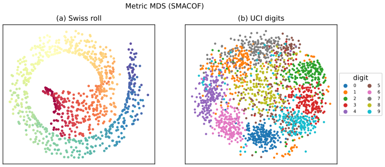
20.4.5 Isomap
p. 694 Two points can be close in space and far along the manifold (Figure 20.32a). Isomap (Tenenbaum et al., 2000) builds the \(K\)-nearest-neighbour graph, approximates the manifold distance by the shortest path along the graph (Dijkstra's algorithm), and then applies classical MDS (PCA) to the resulting squared distances, capturing local structure while avoiding local optima. It works well on the Swiss roll and gives a reasonable picture of the digits (Figure 20.33). With noise there can be "false" edges that join distant layers; these short circuits distort the embedding (Figure 20.34), an instability of topology (Balasubramanian and Schwartz, 2002). A very small neighbourhood does not cure it, since the graph may fragment.
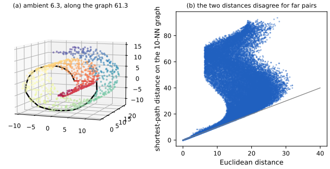
Filling the gap 20.19: why graph distances approximate geodesics, and what goes wrong pp. 694–695, Tenenbaum et al. (2000)
Statement, sketch and numerical evidence
Graph distance against geodesic distance. Let \(\mathcal M\subset\R^D\) be a compact smooth manifold with geodesic distance \(d_{\mathcal M}\), and let the sample be dense enough that every point of \(\mathcal M\) is within \(\delta\) of a sample point and the neighbourhood radius \(\varepsilon\) is small against the curvature radius. Bernstein, de Silva, Langford and Tenenbaum (2000) prove that for all sample points \(\bm x,\bm y\), \((1-\eta)d_{\mathcal M}(\bm x,\bm y)\le d_G(\bm x,\bm y)\le(1+\eta)d_{\mathcal M}(\bm x,\bm y)\) with \(\eta=O(\varepsilon^2\kappa^2+\delta/\varepsilon)\) (\(\kappa\) = maximal curvature). Sketch of the upper bound: pick sample points \(\bm p_0=\bm x,\dots,\bm p_m=\bm y\) within \(\delta\) of the geodesic with consecutive spacing about \(\varepsilon\); each chord is at most the arc length, and shorter than \(\varepsilon\), so it is an edge, and the path length is at most \(d_{\mathcal M}\) plus the \(\delta\)-detours. Sketch of the lower bound: an edge of length \(\ell\le\varepsilon\) joins points whose geodesic distance is at most \(\ell(1+O(\kappa^2\ell^2))\) (a chord of a curve of curvature at most \(\kappa\) is nearly as long as its arc), and by the triangle inequality for \(d_{\mathcal M}\) the sum over the path edges is at least \(d_{\mathcal M}(\bm x,\bm y)\) up to that factor. A trivial inequality always holds: \(d_G\ge\|\bm x-\bm y\|\) because every edge is a Euclidean segment. Figure 20.32 shows both regimes.
Classical MDS of non-Euclidean distances. The matrix \(-\frac12\bm C_N\bm G^{(2)}\bm C_N\) of squared graph distances need not be positive semi-definite, so some eigenvalues may be negative; one keeps the top \(L\) (positive) eigenpairs and ignores the rest. For the roll these are dominant: \(4.0\times10^5\) and \(2.0\times10^4\) against \(5.3\times10^3\) for the third at \(K=6\).
Short circuits. A single wrong edge between layers shortens the shortest paths of all pairs whose paths can use it, so the metric changes globally, not locally. On a 500-point roll the number of edges joining points whose positions along the roll differ by more than 3 radians (short circuits) and the "unrolling score" \(|\mathrm{corr}(z_1,t)|\) for noise 0 are: \(K=6\): 0 edges, 0.991; \(K=10\): 0, 0.991; \(K=14\): 23, 0.275; \(K=20\): 224, 0.165; \(K=30\): 1050, 0.103. With noise of standard deviation 0.5: \(K=6\): 2 edges, 0.819; \(K=10\): 10, 0.541. Smaller \(K\) can still work (\(K=4\) gives 0.990 at that noise) but the graph breaks into components when \(K\) is too small (at \(K=2\) the clean roll has 26 components). The usable \(K\) shrinks as the noise grows: this is the topological instability. Remedies exist (Choi and Choi, 2007). \(\square\)
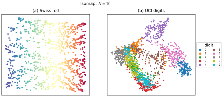
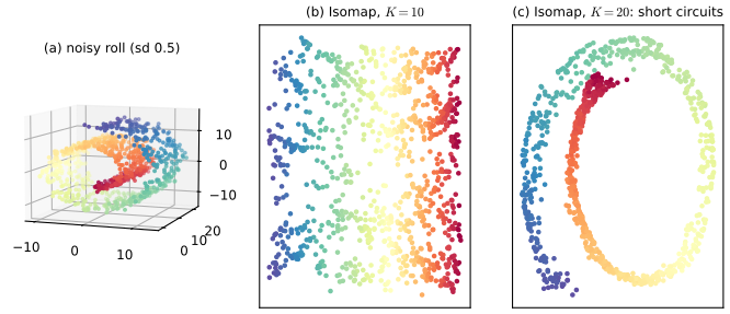
20.4.6 Kernel PCA
pp. 695–697 PCA and classical MDS find the best linear map that preserves similarities. Kernel PCA (Schölkopf et al., 1998) solves PCA through the Gram matrix \(\bm K=\bm X\bm X^\T\) (Section 20.1.3.2) and then applies the kernel trick (Section 17.3.4), replacing \(\bm x_i^\T\bm x_j\) by \(\mathcal K(\bm x_i,\bm x_j)\); by Mercer's theorem this implicitly replaces \(\bm x_i\) by \(\bm\phi(\bm x_i)\). The normalised eigenvectors of the feature covariance \(\bm S_\phi=\frac1N\sum_i\bm\phi_i\bm\phi_i^\T\) are \(\bm V_{\rm kPCA}=\bm\Phi^\T\bm U\bm\Lambda^{-1/2}\) (20.22 in feature space), which cannot be computed since \(\bm\phi\) may be infinite dimensional, but the projection of a new point is computable: \(\bm\phi_*^\T\bm V_{\rm kPCA}=\bm k_*^\T\bm U\bm\Lambda^{-1/2}\) with \(\bm k_*=[\mathcal K(\bm x_*,\bm x_1),\dots,\mathcal K(\bm x_*,\bm x_N)]^\T\) (the book's (20.114)). The features must be centred, which cannot be done explicitly; instead use the double-centred Gram matrix \(\tilde{\bm K}=\bm C_N\bm K\bm C_N\). With a linear kernel one recovers PCA (limited to \(L\le D\) components); with a non-degenerate kernel up to \(N\) components exist. Figure 20.35 shows the first eight kernel principal components of 2-D data in three clusters with an RBF kernel: the first two separate the three clusters and the later ones split the clusters. On the roll and the digits the RBF kernel is arguably not useful (Figure 20.36): kernel PCA with an RBF kernel expands the feature space rather than reducing it (Weinberger et al., 2004).
Filling the gap 20.20: kernel PCA with centring, projection of new points, and why an RBF kernel does not reduce dimension pp. 695–697, (20.114)
Derivation
Eigenvectors and scores. Let \(\tilde{\bm\Phi}\) have rows \(\tilde{\bm\phi}_i=\bm\phi(\bm x_i)-\bar{\bm\phi}\), \(\bar{\bm\phi}=\frac1N\sum_i\bm\phi(\bm x_i)\); the centred Gram matrix has entries \(\tilde K_{ij}=\tilde{\bm\phi}_i^\T\tilde{\bm\phi}_j=K_{ij}-\frac1N\sum_lK_{il}-\frac1N\sum_lK_{lj}+\frac1{N^2}\sum_{lm}K_{lm}\), i.e. \(\tilde{\bm K}=\bm C_N\bm K\bm C_N\), computable from \(\bm K\) alone. Gap 20.3 applied to \(\tilde{\bm\Phi}\) with \(\tilde{\bm K}=\bm U\bm\Lambda\bm U^\T\): the unit eigenvectors of the feature covariance \(\frac1N\tilde{\bm\Phi}^\T\tilde{\bm\Phi}\) are \(\bm v_k=\tilde{\bm\Phi}^\T\bm u_k\lambda_k^{-1/2}\) with variances \(\lambda_k/N\). The score of the training point \(i\) on component \(k\) is \(\tilde{\bm\phi}_i^\T\bm v_k=\lambda_k^{-1/2}(\tilde{\bm K}\bm u_k)_i=\lambda_k^{1/2}u_{ik}\): the rows of \(\bm U\bm\Lambda^{1/2}\), as in classical MDS (Gap 20.18).
A new point. The projection is \(\tilde{\bm\phi}_*^\T\bm v_k=\lambda_k^{-1/2}\tilde{\bm k}_*^\T\bm u_k\), with \(\tilde{\bm\phi}_*=\bm\phi(\bm x_*)-\bar{\bm\phi}\) and \(\tilde k_{*j}=\tilde{\bm\phi}_*^\T\tilde{\bm\phi}_j=k_{*j}-\frac1N\sum_ik_{*i}-\frac1N\sum_iK_{ij}+\frac1{N^2}\sum_{il}K_{il}\). The book gives the formula for uncentred kernels; the test point needs its own centring (subtract its own mean kernel value and the mean of the training Gram matrix), else the new points are not on the same scale as the training points. Numerically: using this formula to project the training points reproduces \(\bm U\bm\Lambda^{1/2}\) to \(10^{-6}\), and the training scores agree with scikit-learn's KernelPCA (up to sign); with the linear kernel \(\mathcal K(\bm x,\bm y)=\bm x^\T\bm y\) the scores are exactly the PCA scores.
The RBF kernel gives full rank. For distinct points \(\bm x_1,\dots,\bm x_N\) the Gaussian Gram matrix \(K_{ij}=e^{-\gamma\|\bm x_i-\bm x_j\|^2}\) is positive definite. Proof: \(e^{-\gamma\|\bm x\|^2}=\int e^{\mathrm i\bm\omega^\T\bm x}g(\bm\omega)\,\d\bm\omega\) with \(g\) a Gaussian density (the characteristic function of a Gaussian), so \(K_{ij}=\int e^{\mathrm i\bm\omega^\T(\bm x_i-\bm x_j)}g(\bm\omega)\,\d\bm\omega\) and \(\bm c^\T\bm K\bm c=\int g(\bm\omega)\big|\sum_jc_je^{\mathrm i\bm\omega^\T\bm x_j}\big|^2\d\bm\omega\ge0\), with equality only if \(\sum_jc_je^{\mathrm i\bm\omega^\T\bm x_j}=0\) for almost every \(\bm\omega\); exponentials in \(\bm\omega\) with distinct frequencies \(\bm x_j\) are linearly independent, so \(\bm c=\bm 0\). Hence all \(N\) eigenvalues of \(\bm K\) are positive (and \(N-1\) of \(\tilde{\bm K}\)): the feature space has dimension at least \(N\) on the data, so there is no dimension reduction, and the leading components may reflect cluster structure or outliers rather than a manifold (Figure 20.36). For the 180 points of Figure 20.35 the RBF Gram matrix has rank 180. The bandwidth matters: with a very narrow kernel \(\bm K\approx\bm I\) and the components are meaningless (the default \(\gamma=1/D\) on the roll and the digits does exactly this); the figures use \(\gamma=1/\mathrm{median}(d_{ij}^2)\). \(\square\)
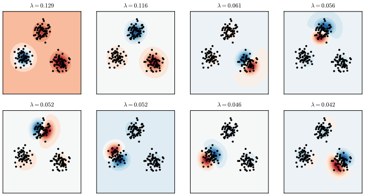
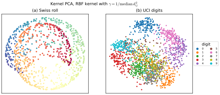
20.4.7 Maximum variance unfolding (MVU)
p. 697 Since an RBF kernel does not reduce dimension, semidefinite embedding or maximum variance unfolding (Weinberger et al., 2004) learns the kernel: find \(\bm z_i\) with \(\max\sum_{ij}\|\bm z_i-\bm z_j\|^2\) subject to \(\|\bm z_i-\bm z_j\|^2=\|\bm x_i-\bm x_j\|^2\) for all neighbour pairs \((i,j)\in G\) (20.115): unfold the manifold as much as possible while keeping the local distances fixed. With \(\bm K=\bm Z\bm Z^\T\) this is the semidefinite program \(\max\Tr(\bm K)\) subject to \(K_{ii}+K_{jj}-2K_{ij}=\|\bm x_i-\bm x_j\|^2\) for \((i,j)\in G\), \(\sum_{ij}K_{ij}=0\), \(\bm K\succeq0\) (20.116); the learned \(\bm K\) is then passed to kernel PCA.
Filling the gap 20.21: why the MVU objective is \(\Tr(\bm K)\) and the problem is a semidefinite program p. 697, (20.115), (20.116)
Derivation
For a centred embedding (\(\sum_i\bm z_i=\bm 0\)) expand \(\sum_{ij}\|\bm z_i-\bm z_j\|^2=\sum_{ij}(\|\bm z_i\|^2+\|\bm z_j\|^2-2\bm z_i^\T\bm z_j)=2N\sum_i\|\bm z_i\|^2-2\|\sum_i\bm z_i\|^2=2N\,\Tr(\bm K)\). Centring is the linear constraint \(\bm 1^\T\bm K\bm 1=\|\sum_i\bm z_i\|^2=0\) (for \(\bm K\succeq0\) this is equivalent to \(\bm K\bm 1=\bm 0\)); the distance constraints \(\|\bm z_i-\bm z_j\|^2=K_{ii}+K_{jj}-2K_{ij}\) are linear in \(\bm K\); and any \(\bm K\succeq0\) factors as \(\bm Z\bm Z^\T\). So the problem is: maximise a linear function over a spectrahedron, a semidefinite program, convex, with a global optimum (no local optima, unlike many other manifold methods). The constraint should read \(\bm K\succeq0\), not \(\bm K\succ0\) as printed in (20.116): a Gram matrix of low-rank embedded data is singular (the \(\succ\) would exclude the solutions of interest, whose rank is the intrinsic dimension). Why it unfolds: trace maximisation spreads the points as far apart as the fixed local distances allow, which pulls a folded sheet flat, and the rank of the solution reveals the dimension. The cost, an SDP in \(N\times N\) variables, limits MVU to a few thousand points. We did not run MVU (no SDP solver in the toolchain). \(\square\)
20.4.8 Local linear embedding (LLE)
pp. 697–698 The preceding methods diagonalise a full matrix of similarities. Locally linear embedding (Roweis and Saul, 2000) solves a sparse eigenproblem and so concentrates on local structure. It assumes the manifold is locally linear: each point is predicted as an affine combination of its \(K\) nearest neighbours, \[ \hat{\bm W}=\arg\min_{\bm W}\sum_i\Big\|\bm x_i-\sum_jw_{ij}\bm x_j\Big\|^2\ \ \text{s.t.}\ \ w_{ij}=0\ \text{if}\ \bm x_j\notin\mathrm{nbr}(\bm x_i,K),\ \ \sum_jw_{ij}=1 , \tag{20.117, 20.118} \] (the sum-to-one constraint rules out \(\bm W=\bm 0\)); the weights are the barycentric coordinates of \(\bm x_i\). Any linear map of the neighbourhood to a lower-dimensional space preserves them, so the embedding keeps the weights fixed: \[ \hat{\bm Z}=\arg\min_{\bm Z}\sum_i\Big\|\bm z_i-\sum_j\hat w_{ij}\bm z_j\Big\|^2=\arg\min_{\bm Z}\,\|\bm Z-\hat{\bm W}\bm Z\|_F^2=\arg\min\Tr\big(\bm Z^\T(\bm I-\hat{\bm W})^\T(\bm I-\hat{\bm W})\bm Z\big) , \tag{20.119, 20.120} \] solved by the eigenvectors of \((\bm I-\hat{\bm W})^\T(\bm I-\hat{\bm W})\) for the smallest nonzero eigenvalues (Section 7.4.8). On the running examples LLE is not as good as Isomap, but tends to be less sensitive to short circuits (Figure 20.37).
Filling the gap 20.22: the closed-form LLE weights, and the constraints that the embedding step needs pp. 697–698, (20.117)–(20.120)
Derivation
Weights. For point \(i\) with neighbours \(j_1,\dots,j_K\), let \(\bm G\in\R^{K\times K}\) be the local Gram matrix \(G_{ab}=(\bm x_{j_a}-\bm x_i)^\T(\bm x_{j_b}-\bm x_i)\). Because \(\sum_aw_a=1\), \(\bm x_i-\sum_aw_a\bm x_{j_a}=-\sum_aw_a(\bm x_{j_a}-\bm x_i)\), so the error is \(\bm w^\T\bm G\bm w\). Minimise under \(\bm 1^\T\bm w=1\): the Lagrangian \(\bm w^\T\bm G\bm w-2\lambda(\bm 1^\T\bm w-1)\) gives \(\bm G\bm w=\lambda\bm 1\), so \[ \bm w=\frac{\bm G^{-1}\bm 1}{\bm 1^\T\bm G^{-1}\bm 1} . \] If \(K>D\) the matrix \(\bm G\) is singular (the neighbours lie in a \(D\)-dimensional space), and in practice one solves with \(\bm G+\epsilon\Tr(\bm G)\bm I\), \(\epsilon=10^{-3}\). If \(\bm x_i\) lies in the affine hull of its neighbours the minimum error is 0 (checked: with an exact affine combination of four points in the plane the formula returns the weights that reconstruct \(\bm x_i\) to \(10^{-8}\)). The weights are invariant to rotation, translation and common rescaling of the neighbourhood (\(\bm w^\T\bm G\bm w\) just rescales), which is why they describe local geometry.
Embedding. Put \(\bm M=(\bm I-\bm W)^\T(\bm I-\bm W)\succeq0\). The cost \(\Phi(\bm Z)=\Tr(\bm Z^\T\bm M\bm Z)\) is minimised at \(\bm Z=\bm 0\), so the book's (20.119) needs constraints, which it does not state: centring \(\bm 1^\T\bm Z=\bm 0\) and unit covariance \(\frac1N\bm Z^\T\bm Z=\bm I_L\). Since every row of \(\bm W\) sums to 1, \(\bm W\bm 1=\bm 1\), \(\bm M\bm 1=\bm 0\): the constant vector is the eigenvector with eigenvalue 0 (the "trivial" solution; checked numerically, the smallest eigenvalue is \(10^{-17}\)). Under the constraints, by the Ky Fan principle the minimum of \(\Tr(\bm Z^\T\bm M\bm Z)\) over \(\bm Z\) with orthonormal columns orthogonal to \(\bm 1\) is the sum of the next \(L\) smallest eigenvalues, attained at the corresponding eigenvectors (scaled by \(\sqrt N\)). There can be more than one zero eigenvalue if the graph is disconnected. The eigenproblem is sparse because \(\bm W\) has \(K\) nonzeros per row. The scikit-learn implementation, run on the same data, agrees with this construction up to sign. \(\square\)
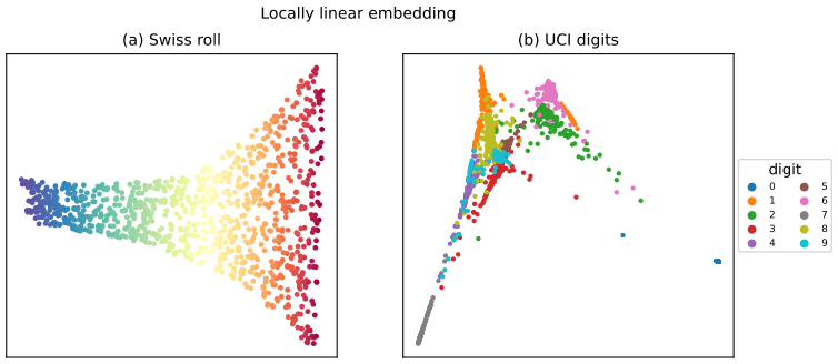
20.4.9 Laplacian eigenmaps
pp. 699–701 Laplacian eigenmaps or spectral embedding (Belkin and Niyogi, 2001) find embeddings in which weighted distances between a point and its neighbours are small, with more weight on the closest. Minimise \[ \mathcal L(\bm Z)=\sum_{(i,j)\in E}W_{ij}\|\bm z_i-\bm z_j\|^2,\qquad W_{ij}=\exp\Big(-\frac{\|\bm x_i-\bm x_j\|^2}{2\sigma^2}\Big)\ \text{for neighbours, 0 otherwise} , \tag{20.121} \] subject to \(\bm Z^\T\bm D\bm Z=\bm I\) with \(\bm D=\diag(\sum_jW_{ij})\) the degree matrix. In matrix form \(\mathcal L=2\Tr(\bm Z^\T\bm D\bm Z)-2\Tr(\bm Z^\T\bm W\bm Z)=2\Tr(\bm Z^\T\bm L\bm Z)\) (20.122–20.124) with the graph Laplacian \(\bm L=\bm D-\bm W\); the minimisers solve the generalised eigenproblem \(\bm L\bm z=\lambda\bm D\bm z\) for the smallest nonzero eigenvalues. The graph Laplacian. For a symmetric non-negative weight matrix, \(L_{ii}=d_i\) and \(L_{ij}=-w_{ij}\) for \(i\ne j\) (20.125, 20.126); for a function \(f\) on the nodes, \((\bm L\bm f)_i=\sum_jw_{ij}[f_i-f_j]\) acts as a discrete derivative (20.127), and the Dirichlet energy \(\bm f^\T\bm L\bm f=\frac12\sum_{ij}w_{ij}(f_i-f_j)^2\) (20.128, 20.129) measures its smoothness. \(\bm L\) is symmetric and positive semi-definite, with eigenvalues \(0\le\lambda_1\le\dots\le\lambda_N\), and its eigenvectors are the basis of functions on the graph in order of decreasing smoothness; the embedding coordinates are these smooth functions (Figures 20.39 and 20.40 are illustrations).
Filling the gap 20.23: Laplacian eigenmaps as a generalised eigenproblem; the Dirichlet energy; connected components pp. 699–701, (20.121)–(20.129)
Proof
Dirichlet energy. \(\frac12\sum_{ij}w_{ij}(f_i-f_j)^2=\frac12\sum_{ij}w_{ij}f_i^2+\frac12\sum_{ij}w_{ij}f_j^2-\sum_{ij}w_{ij}f_if_j=\sum_id_if_i^2-\bm f^\T\bm W\bm f=\bm f^\T(\bm D-\bm W)\bm f\) (20.128, 20.129), using symmetry. Since \(w_{ij}\ge0\), \(\bm f^\T\bm L\bm f\ge0\): \(\bm L\) is positive semi-definite and has real non-negative eigenvalues. Applying this columnwise to \(\bm Z\) gives (20.122)–(20.124): \(\sum_{ij}W_{ij}\|\bm z_i-\bm z_j\|^2=2\Tr(\bm Z^\T\bm L\bm Z)\) (the book's (20.121) sums over edges, the identity holds with the sum over ordered pairs).
The optimisation. Minimise \(\Tr(\bm Z^\T\bm L\bm Z)\) subject to \(\bm Z^\T\bm D\bm Z=\bm I_L\). Put \(\bm Y=\bm D^{1/2}\bm Z\) (needs \(d_i>0\)): the problem becomes minimise \(\Tr(\bm Y^\T\bm L_{\rm sym}\bm Y)\) with \(\bm Y^\T\bm Y=\bm I\), where \(\bm L_{\rm sym}=\bm D^{-1/2}\bm L\bm D^{-1/2}\). By the Ky Fan principle (Gap 20.1 with the sign reversed) the minimum is the sum of the \(L\) smallest eigenvalues, attained at the corresponding eigenvectors \(\bm y_k\), i.e. \(\bm z_k=\bm D^{-1/2}\bm y_k\), which satisfy \(\bm L\bm z_k=\lambda_k\bm D\bm z_k\) (the generalised problem). The first eigenvalue is 0 with \(\bm z=\bm 1\) (since \(\bm L\bm 1=\bm 0\)): the constant function is smoothest but carries no information, and corresponds to the trivial embedding \(\bm Z=\bm 1\); it is discarded, leaving the eigenvectors of the next \(L\) eigenvalues. The eigenvalue is the Rayleigh quotient \(\lambda_k=\bm z_k^\T\bm L\bm z_k/\bm z_k^\T\bm D\bm z_k\), the Dirichlet energy relative to the weighted mass (Figure 20.S3 prints both and they coincide). Equivalently, \(\bm D^{-1}\bm W\bm z=(1-\lambda)\bm z\): the embedding uses the eigenvectors of the random-walk transition matrix with the largest eigenvalues.
Connected components. \(\bm f^\T\bm L\bm f=0\) iff \(f_i=f_j\) whenever \(w_{ij}>0\), i.e. iff \(\bm f\) is constant on each connected component; so the multiplicity of the eigenvalue 0 equals the number of connected components of the graph (checked on a graph with three components, which has exactly three zero eigenvalues). If the neighbourhood graph is disconnected the first embedding coordinates just label the components, so \(K\) must be chosen to connect the graph. As \(N\to\infty\) with a suitably shrinking bandwidth, the eigenvectors converge to eigenfunctions of the Laplace–Beltrami operator of the manifold (Belkin and Niyogi, 2003); this is quoted, not reproved. On the Swiss roll the smoothest nonconstant functions depend almost only on the position \(t\) along the roll, like \(\cos(\pi s)\), \(\cos(2\pi s)\), \(\cos(3\pi s)\) with \(s\) the scaled coordinate along the length (Figure 20.S3); the first two coordinates therefore trace a parabola (\(\cos2\pi s=2\cos^2\pi s-1\)), the U-shaped curve of Figure 20.38a, which orders the points along the roll but does not unroll it into a rectangle. \(\square\)
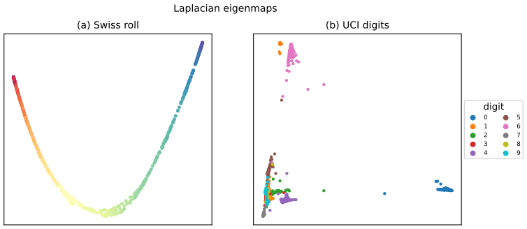
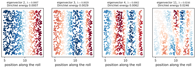
20.4.10 t-SNE
pp. 701–705 t-SNE (van der Maaten and Hinton, 2008) is a popular nonconvex method for 2-D or 3-D visualisation; it extends stochastic neighbour embedding (SNE; Hinton and Roweis, 2003).
20.4.10.1 Stochastic neighbourhood embedding (SNE)
pp. 701–702 Convert distances into conditional probabilities: \(p_{j\mid i}\) is the probability that \(i\) picks \(j\) as a neighbour if neighbours are chosen in proportion to a Gaussian centred at \(\bm x_i\), \[ p_{j\mid i}=\frac{\exp(-\frac1{2\sigma_i^2}\|\bm x_i-\bm x_j\|^2)}{\sum_{k\ne i}\exp(-\frac1{2\sigma_i^2}\|\bm x_i-\bm x_k\|^2)} , \tag{20.130} \] with a point-specific variance \(\sigma_i^2\) (large in sparse regions). Define \(q_{j\mid i}=\exp(-\|\bm z_i-\bm z_j\|^2)/\sum_{k\ne i}\exp(-\|\bm z_i-\bm z_k\|^2)\) (20.131) (a fixed variance, since changing it only rescales the map) and minimise \(\sum_i\KL(P_i\|Q_i)=\sum_i\sum_jp_{j\mid i}\log\frac{p_{j\mid i}}{q_{j\mid i}}\) (20.132). It is asymmetric: a small \(q_{j\mid i}\) used for a large \(p_{j\mid i}\) is expensive, so it prefers to pull distant points together rather than to push nearby points apart, and the gradient \[ \nabla_{\bm z_i}\mathcal L=2\sum_j(\bm z_i-\bm z_j)\big(p_{j\mid i}-q_{j\mid i}+p_{i\mid j}-q_{i\mid j}\big) \tag{20.133} \] attracts points when the \(p\)'s exceed the \(q\)'s and repels them otherwise. The objective is not convex; it can be minimised by SGD, with Gaussian noise added to the embedding and annealed (Hinton recommends spending long at the noise level at which global structure forms).
20.4.10.2 Symmetric SNE
pp. 702–703 A simpler version minimises one KL between the joint distributions, \(\mathcal L=\KL(P\|Q)=\sum_{i<j}p_{ij}\log\frac{p_{ij}}{q_{ij}}\) (20.134), with \(p_{ij}\propto\exp(-\frac1{2\sigma^2}\|\bm x_i-\bm x_j\|^2)\) (20.135) (in practice \(p_{ij}=(p_{j\mid i}+p_{i\mid j})/2N\) so that every point has a say) and \(q_{ij}\) defined likewise; its gradient is \(4\sum_j(\bm z_i-\bm z_j)(p_{ij}-q_{ij})\) (20.136). It loses the property of SNE that if \(L=D\) the data are their own optimal embedding, but gives similar results in practice.
20.4.10.3 t-distributed SNE
p. 703 SNE and many other embeddings suffer from crowding: moderately far points in the high-dimensional space are squeezed together in the 2-D map, because the Gaussian is too light-tailed. t-SNE uses a Student-\(t\) with \(\nu=1\) degree of freedom, i.e. a Cauchy, in the map, \[ q_{ij}=\frac{(1+\|\bm z_i-\bm z_j\|^2)^{-1}}{\sum_{k<l}(1+\|\bm z_k-\bm z_l\|^2)^{-1}} , \tag{20.137} \] with the same objective (20.134). The gradient is \(\nabla_{\bm z_i}\mathcal L=4\sum_j(p_{ij}-q_{ij})(\bm z_i-\bm z_j)(1+\|\bm z_i-\bm z_j\|^2)^{-1}\) (20.138), that of Gaussian symmetric SNE with the extra factor \((1+d^2)^{-1}\), which acts as an inverse-square law so that points in the map behave like stars and galaxies: well-separated clusters each with tightly packed members (Figure 20.41).
Filling the gap 20.24: the gradients of SNE, symmetric SNE and t-SNE pp. 702–703, (20.133), (20.136), (20.138)
Derivation
Symmetric SNE and t-SNE. Let \(k(d)\) be the map kernel (\(k=e^{-d^2}\) for Gaussian SNE, \(k=(1+d^2)^{-1}\) for t-SNE), \(k_{ij}=k(\|\bm z_i-\bm z_j\|)\), \(Z=\sum_{k\ne l}k_{kl}\) and \(q_{ij}=k_{ij}/Z\), with \(p\) normalised over ordered pairs, \(\sum_{i\ne j}p_{ij}=1\). Then \(\mathcal L=\sum_{i\ne j}p_{ij}\log p_{ij}-\sum_{i\ne j}p_{ij}\log k_{ij}+\log Z\) (using \(\sum p_{ij}=1\)). The variable \(\bm z_i\) enters \(k_{ij}\) and \(k_{ji}\) for each \(j\), and \(k_{ij}=k_{ji}\), so \[ \nabla_{\bm z_i}\mathcal L=-2\sum_jp_{ij}\nabla_{\bm z_i}\log k_{ij}+\frac1Z\cdot2\sum_j\nabla_{\bm z_i}k_{ij}=2\sum_j(q_{ij}-p_{ij})\nabla_{\bm z_i}\log k_{ij} . \] For the Gaussian kernel \(\nabla_{\bm z_i}\log k_{ij}=-2(\bm z_i-\bm z_j)\), giving \(4\sum_j(p_{ij}-q_{ij})(\bm z_i-\bm z_j)\) (20.136). For the Cauchy kernel \(\log k=-\log(1+d^2)\), so \(\nabla_{\bm z_i}\log k_{ij}=-\frac{2(\bm z_i-\bm z_j)}{1+d_{ij}^2}\), giving \(4\sum_j(p_{ij}-q_{ij})(\bm z_i-\bm z_j)(1+d_{ij}^2)^{-1}\) (20.138). Normalisation convention: the factor 4 holds when the pairs are counted in both orders. With the book's \(\sum_{i<j}\) in (20.134), normalising \(P\) and \(Q\) over unordered pairs gives \(P^u=2p\), \(Q^u=2q\); the loss \(\sum_{i<j}P^u_{ij}\log\frac{P^u_{ij}}{Q^u_{ij}}=\sum_{i\ne j}p_{ij}\log\frac{p_{ij}}{q_{ij}}\) is the same function of \(\bm Z\), so its gradient is \(2\sum_j(P^u_{ij}-Q^u_{ij})(\bm z_i-\bm z_j)\) (times \((1+d_{ij}^2)^{-1}\) for t-SNE): the book's (20.136) and (20.138) are right with ordered-pair normalisation, while (20.135) normalises over \(k\ne l\) and (20.137) over \(k<l\). Both gradients were confirmed against finite differences, as was the asymmetric one below.
Asymmetric SNE. \(\mathcal L=\sum_i\sum_jp_{j\mid i}\log\frac{p_{j\mid i}}{q_{j\mid i}}\) and \(\mathcal L_i=\sum_jp_{j\mid i}d_{ij}^2+\log\sum_ke^{-d_{ik}^2}+\mathrm{const}\) (using \(\sum_jp_{j\mid i}=1\) and \(d_{ij}=\|\bm z_i-\bm z_j\|\)). Treating the squared distances \(d_{ij}^2\) as free variables, \(\partial\mathcal L/\partial d_{ij}^2=p_{j\mid i}-q_{j\mid i}\) (the softmax derivative). Since \(\partial d_{ij}^2/\partial\bm z_i=2(\bm z_i-\bm z_j)\), and \(\bm z_i\) appears both in its own row \(i\) (as \(d_{ij}^2\)) and in every other row \(j\) (as \(d_{ji}^2=d_{ij}^2\)), \(\nabla_{\bm z_i}\mathcal L=\sum_j\big[(p_{j\mid i}-q_{j\mid i})+(p_{i\mid j}-q_{i\mid j})\big]\,2(\bm z_i-\bm z_j)\), which is (20.133). In all three cases the gradient is a sum of forces along the line between points, attractive when \(p\) exceeds \(q\) and repulsive otherwise. Why the t-kernel helps: to represent a small neighbour probability \(p_0\) the Gaussian map needs the distance \(d=\sqrt{\log(1/p_0)}\), the Cauchy map \(d\approx1/\sqrt{p_0}\) (for the same normaliser); the heavy tail lets moderately dissimilar points sit far apart in the map instead of being squeezed (Figure 20.S4). \(\square\)
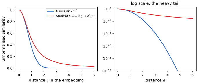
20.4.10.4 Choosing the length scale
p. 704 The local bandwidth \(\sigma_i^2\) is set so that \(P_i\) has a given perplexity \(2^{H(P_i)}\), \(H(P_i)=-\sum_jp_{j\mid i}\log_2p_{j\mid i}\) (Section 6.1.5): roughly the effective number of neighbours. Results depend on the perplexity, so one should try several values (Figure 20.42: with perplexity too small the method finds structure inside clusters that is not there; at the scikit-learn default of 30 the clusters look equidistant even if some are closer; see Wattenberg et al., 2016, for other cautions).
Filling the gap 20.25: the perplexity search is well posed (entropy is monotone in the bandwidth) p. 704, footnote 7
Proof
Fix \(i\) and write \(e_j=\|\bm x_i-\bm x_j\|^2\) and \(\beta=1/(2\sigma_i^2)\). Then \(p_{j\mid i}=e^{-\beta e_j}/Z(\beta)\), \(Z=\sum_je^{-\beta e_j}\), a Gibbs distribution with energies \(e_j\) and inverse temperature \(\beta\). Its entropy (natural logarithm) is \(H(\beta)=\beta\,\E_\beta[e]+\log Z(\beta)\). Since \((\log Z)'=-\E_\beta[e]\) and \(\E_\beta[e]'=-\mathrm{Var}_\beta(e)\), \[ H'(\beta)=\E_\beta[e]+\beta(-\mathrm{Var}_\beta(e))-\E_\beta[e]=-\beta\,\mathrm{Var}_\beta(e)<0 \] whenever the distances \(e_j\) are not all equal: the entropy is strictly decreasing in \(\beta\), from \(\log(N-1)\) at \(\beta=0\) (uniform) to the log of the number of tied nearest neighbours as \(\beta\to\infty\). Hence for every target perplexity strictly between those values there is exactly one \(\beta\) (hence one \(\sigma_i\)), and bisection finds it (the code brackets \(\beta\) by doubling and halving). The perplexity \(2^{H}\) (or \(e^{H}\) in nats) is the number of equiprobable neighbours that would have the same entropy: a uniform distribution on \(m\) points has perplexity \(m\). Numerically \(dH/d\beta\) matches \(-\beta\mathrm{Var}(e)\) to six digits. In the examples: the 150 points of three clusters with perplexity 5 get a mean \(\sigma_i\) of 0.099 and with perplexity 30 of 0.30 (the clusters have 50 points each, so perplexity 30 already sees most of the own cluster); 300 digits at perplexity 30 get 12.0. \(\square\)
20.4.10.5 Computational issues
p. 705 A naive implementation costs \(O(N^2)\) per iteration (the gradient sums over all pairs). Treating distant points as groups, as in an \(N\)-body simulation, the Barnes–Hut approximation (Barnes and Hut, 1986) reduces this to \(O(N\log N)\) (van der Maaten, 2014), but works well only for low-dimensional embeddings (\(L=2\) or 3).
20.4.10.6 UMAP
p. 705 UMAP (McInnes et al., 2018) is similar to t-SNE, tends to preserve global structure better and is much faster, which makes it easy to try several hyperparameters (see Coenen and Pearce, 2019, for an interactive comparison).
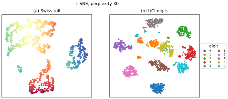
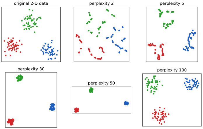
20.5 Word embeddings
pp. 705–712 Words are categorical variables, so their one-hot vectors \(\bm s_{n,t}\in\{0,1\}^M\) are sparse and carry no similarity: "man" and "woman" are at Hamming distance 1, and so are "man" and "banana". A word embedding maps each word to a dense vector \(\bm z\in\R^D\) so that semantically similar words are close, which also eases data sparsity. Similarity is defined by the distributional hypothesis (Harris, 1954): words are similar if they occur in similar contexts ("a word is characterised by the company it keeps", Firth, 1957). All methods below learn a map from a word's contexts to a vector; all of them, as Section 20.5.5 explains, factorise (implicitly or explicitly) a matrix of pointwise mutual information.
See also: the embedding of tokens and the transformer in Foundations of Deep Learning, Chapter 12; contextual embeddings are Section 15.7 of the book (Chapter 15 of these notes).
20.5.1 Latent semantic analysis / indexing
20.5.1.1 Latent semantic indexing (LSI)
pp. 705–706 Let \(C_{ij}\) be the number of times term \(i\) occurs in context \(j\) (here: document \(j\) of a corpus; possibly after the TF-IDF transformation of Section 1.5.4.2). The rank-\(K\) matrix \(\hat{\bm C}\) minimising \(\mathcal L(\hat{\bm C})=\|\bm C-\hat{\bm C}\|_F^2\) (20.139) is the truncated SVD \(\hat{\bm C}=\bm U\bm S\bm V^\T\) (the book writes \(\bm V\) for \(\bm V^\T\)), i.e. the bilinear model \(c_{ij}\approx\sum_{k=1}^Ku_{ik}s_kv_{jk}\) (20.140). The vector \(\bm u_i\) is the embedding of word \(i\) and \(\bm s\odot\bm v_j\) that of context \(j\). For latent semantic indexing (Deerwester et al., 1990) a query, a bag of words \(w_1,\dots,w_B\), is represented by \(\bm q=\frac1B\sum_b\bm u_{w_b}\) and documents are ranked by the cosine similarity \(\mathrm{sim}(\bm q,\bm d)=\bm q^\T\bm d/(\|\bm q\|\|\bm d\|)\) (20.141) with the document vectors. For unit vectors the cosine is the inner product and equals \(1-\frac12\|\bm q-\bm d\|^2\), i.e. squared distance up to sign and a constant: \(\|\bm q-\bm d\|^2=2(1-\mathrm{sim}(\bm q,\bm d))\) (20.142).
20.5.1.2 Latent semantic analysis (LSA)
p. 707 If the context is a local neighbourhood of words (a window of size \(h\)) instead of a document, \(C_{ij}\) counts how often word \(i\) occurs in a neighbourhood of type \(j\) and the same SVD gives latent semantic analysis (Deerwester et al., 1990). On the British National Corpus (the book cites Eisenstein, 2019), the nearest neighbours of "dog" by cosine are: window \(h=2\): cat, horse, fox, pet, rabbit, pig, animal, mongrel, sheep, pigeon; window \(h=30\): kennel, puppy, pet, bitch, terrier, rottweiler, canine, cat, to bark. The short window is more sensitive to syntax, the long one to semantics.
20.5.1.3 PMI
p. 707 In practice replacing counts by pointwise mutual information gives much better embeddings: \[ \PMI(i,j)=\log\frac{p(i,j)}{p(i)\,p(j)} , \tag{20.143} \] positive when \(i\) and \(j\) co-occur more often than if independent. Negative PMI values are unreliable, so one uses the positive PMI \(\mathrm{PPMI}(i,j)=\max(\PMI(i,j),0)\) (Bullinaria and Levy, 2007), and the SVD of the PPMI matrix yields embeddings that do well on word-meaning tasks.
Filling the gap 20.26: why the truncated SVD, how new queries are embedded, and what the cosine measures pp. 705–707, (20.139)–(20.142)
Derivation
Optimality. The statement "the minimiser of (20.139) is the rank-\(K\) truncated SVD" is the Eckart–Young–Mirsky theorem, proved in Result 7.5; the minimum is \(\sum_{k>K}s_k^2\). The same argument as for PCA (Gap 20.1) shows that the optimal subspace of term space is spanned by the top \(K\) left singular vectors, and \(\hat{\bm C}=\bm U_K(\bm U_K^\T\bm C)\) is the projection of every document column on it. On the synthetic corpus of Figure 20.45 the rank-3 truncation has an error equal to the sum of the discarded \(s_k^2\) (checked), and no random rank-3 projection of 100 tried does better.
Folding in. A new context with count vector \(\bm c\in\R^M\) is represented by the coordinates \(\bm y\) that minimise \(\|\bm c-\bm U_K\bm y\|^2\): \(\bm y=\bm U_K^\T\bm c\). For an existing document \(\bm c=\bm C_{:,j}=\bm U\bm S\bm v_j\), so \(\bm y=\bm S\bm v_j\), exactly the context embedding \(\bm s\odot\bm v_j\) of the text. The reconstructed association of word \(i\) with context \(j\) is \(\bm u_i^\T\bm S\bm v_j\), so a query \(\bm q\) built from word vectors \(\bm u\) is naturally compared with the contexts as \(\bm q^\T\bm S\bm v_j\); comparing \(\bm q\) with \(\bm v_j\) directly, as in the text, uses a different weighting of the latent dimensions (both are used in practice).
The cosine. For \(\|\bm q\|=\|\bm d\|=1\), \(\|\bm q-\bm d\|^2=\bm q^\T\bm q+\bm d^\T\bm d-2\bm q^\T\bm d=2(1-\bm q^\T\bm d)\) (20.142); so ranking by cosine is ranking by Euclidean distance after normalising the vectors, and the cosine is insensitive to the length of a document (which grows with its size).
PMI. With \(\hat p(i,j)=C_{ij}/T\), \(T=\sum_{ij}C_{ij}\), \(\hat p(i)=\sum_jC_{ij}/T\), \(\hat p(j)=\sum_iC_{ij}/T\), the empirical PMI is \(\log\frac{TC_{ij}}{C_{i\cdot}C_{\cdot j}}\), \(-\infty\) for unseen pairs; truncating at 0 gives PPMI (a finite, non-negative matrix with the same sparsity as \(\bm C\)). \(\square\)
20.5.2 Word2vec
pp. 707–710 Word2vec (Mikolov et al., 2013a, b) is a pair of shallow networks that predict a word from its context. CBOW (continuous bag of words, Figure 20.44a, a diagram) predicts each word from the average \(\bm v_t=\frac1{2m}\sum_{h=1}^m(\bm v_{w_{t+h}}+\bm v_{w_{t-h}})\) of the vectors in a window of half-width \(m\) (20.146): \[ \log p(\bm w)=\sum_{t=1}^T\log p(w_t\given w_{t-m:t+m})=\sum_t\Big[\bm v_{w_t}^\T\bm v_t-\log\sum_{i\in\mathcal V}\exp(\bm v_i^\T\bm v_t)\Big] . \tag{20.144, 20.145} \] Skip-gram (Figure 20.44b) predicts the context from each word: the loss is \(-\log p(\bm w)=-\sum_t\sum_{-m\le j\le m,\,j\ne0}\log p(w_{t+j}\given w_t)\) (20.147, 20.148) with a softmax over the vocabulary \[ \log p(w_o\given w_c)=\bm u_o^\T\bm v_c-\log\sum_{i\in\mathcal V}\exp(\bm u_i^\T\bm v_c) , \tag{20.149} \] where \(\bm v_i\) is the embedding of word \(i\) as a centre word and \(\bm u_i\) as a context word. The normaliser over the whole vocabulary makes the likelihood and its gradient expensive. Skip-gram with negative sampling (SGNS; Mikolov et al., 2013b) replaces it by a binary classification: for each centre word \(w_t\) take the \(K+1\) context words, the true \(w_{t+j}\) labelled positive and \(K\) noise words \(w_k\sim p(w)\propto\mathrm{freq}(w)^{3/4}\) (which moves mass from common to rare words) labelled negative: \[ p(w_{t+j}\given w_t)\approx p(D=1\given w_t,w_{t+j})\prod_{k=1}^Kp(D=0\given w_t,w_k) \tag{20.150} \] with \(p(D=1\given w_t,w_{t+j})=\sigma(\bm u_{w_{t+j}}^\T\bm v_{w_t})\) and \(p(D=0\given w_t,w_k)=1-\sigma(\bm u_{w_k}^\T\bm v_{w_t})\) (20.151, 20.152); the embeddings are trained by SGD on the log of this probability.
Filling the gap 20.27: skip-gram with negative sampling factorises a shifted PMI matrix; the GloVe objective pp. 707–710, (20.149)–(20.156); Levy and Goldberg (2014)
Derivation
The softmax gradient. From (20.149), \(\nabla_{\bm v_c}\log p(w_o\given w_c)=\bm u_o-\sum_ip(i\given w_c)\bm u_i\): observed context vector minus the model-expected one, with a cost \(O(|\mathcal V|)\) per pair, the reason for negative sampling.
The expected SGNS objective. Let \(n(w,c)\) count the observed (centre \(w\), context \(c\)) pairs, \(n(w)=\sum_cn(w,c)\), and \(P_n(c)\) the noise distribution. Over the corpus the objective (the log of (20.150) summed over pairs) is, in expectation over the noise words, \[ \mathcal J=\sum_{w,c}\Big[n(w,c)\log\sigma(x_{wc})+K\,n(w)P_n(c)\log\sigma(-x_{wc})\Big],\qquad x_{wc}=\bm u_c^\T\bm v_w . \] If the dimension is large enough that the scores \(x_{wc}\) are free parameters, \(\mathcal J\) separates over pairs. Each summand \(f(x)=a\log\sigma(x)+b\log\sigma(-x)\) with \(a=n(w,c)\), \(b=Kn(w)P_n(c)\) is strictly concave with \(f'(x)=a\sigma(-x)-b\sigma(x)=0\) at \(e^x=a/b\), so \[ x^*_{wc}=\log\frac{n(w,c)}{K\,n(w)P_n(c)}=\log\frac{p(c\given w)}{P_n(c)}-\log K . \] If the noise distribution is the unigram distribution \(P_n(c)=p(c)\), this is \(x^*_{wc}=\PMI(w,c)-\log K\): SGNS implicitly factorises the PMI matrix shifted by \(\log K\) (and with the \(3/4\)-power noise a PMI-like quantity); with a rank-\(L\) constraint it is a weighted low-rank approximation of that matrix, where the weight of pair \((w,c)\) is the expected number of times it is trained. For pairs never observed, \(a=0\) and \(x^*=-\infty\): they are pushed to large negative scores, the analogue of the truncation to PPMI. I verified the stationary point numerically (a bounded scalar optimisation reproduces \(\log(a/b)\) to \(10^{-6}\)). This is the link to Section 20.5.1.3 and to the RAND-WALK explanation of the empirical success of SVD on PPMI matrices.
From skip-gram to GloVe. Let \(x_{ij}\) count how often word \(j\) occurs in a window of word \(i\) and \(x_i=\sum_jx_{ij}\). The skip-gram loss (20.148) is \(-\sum_{i}\sum_jx_{ij}\log q_{ij}\) with \(q_{ij}\) the softmax (20.153) (20.154); writing \(p_{ij}=x_{ij}/x_i\) gives \(\mathcal L=-\sum_ix_i\sum_jp_{ij}\log q_{ij}\) (20.155), a cross-entropy between the empirical and model context distributions, weighted by the word's frequency (checked numerically on random counts). The softmax normaliser is expensive, so GloVe (Pennington et al., 2014) fits the unnormalised model \(q'_{ij}=\exp(\bm u_j^\T\bm v_i+b_i+c_j)\) (the biases absorb the marginals) to the unnormalised target \(x_{ij}\) on the log scale with a weighted square loss, which is more robust than the log loss to errors in small probabilities, and down-weights rare pairs with \(h(x)=(x/x_{\max})^{0.75}\) for \(x<x_{\max}=100\) and 1 otherwise: \[ \mathcal L=\sum_{i,j\in\mathcal V}h(x_{ij})\big(\bm u_j^\T\bm v_i+b_i+c_j-\log x_{ij}\big)^2 . \tag{20.156} \] The book prints this with a leading minus sign, which would make the objective a negative sum of squares, unbounded below under minimisation; the sign must be \(+\). Since \(h(0)=0\) the pairs with \(x_{ij}=0\) are skipped, so \(\log0\) never appears. The final embedding of word \(i\) is \(\frac12(\bm v_i+\bm u_i)\). A perfect fit would mean \(\log x_{ij}=\bm u_j^\T\bm v_i+b_i+c_j\): a low-rank structure for the log-count matrix, the same kind of statement as for SGNS and the PMI. \(\square\)
20.5.3 GloVe
p. 710 GloVe is an alternative to skip-gram with a simpler, faster objective (20.156), derived in Gap 20.27: weighted least squares on the log co-occurrence counts, precomputed offline and optimised by SGD. It gives results similar to skip-gram and is faster to train.
20.5.4 Word analogies
pp. 710–711 Embeddings from word2vec, GloVe and similar methods capture relational meaning through vector addition. For the analogy "man is to woman as king is to queen" (\(a\!:\!b::c\!:\!d\)), let \(\bm\delta=\bm v_b-\bm v_a\) be the "gender change" vector and find the vocabulary word nearest to \(\bm v_c+\bm\delta\) (the 3CosAdd rule; Figure 20.45). Pennington et al. (2014) conjecture that \(a\!:\!b::c\!:\!d\) holds iff for every word \(w\) \[ \frac{p(w\given a)}{p(w\given b)}\approx\frac{p(w\given c)}{p(w\given d)} , \tag{20.157} \] and Arora et al. (2016) show that this follows from the RAND-WALK assumptions below (see also Allen and Hospedales, 2019; Ethayarajh et al., 2019).
20.5.5 RAND-WALK model of word embeddings
pp. 711–712 A simple generative model of text, after Arora et al. (2016), explains why embeddings work. Each word \(w_t\) is generated from a latent context (discourse) vector \(\bm z_t\in\R^D\) by a log-bilinear language model, \[ p(w_t=w\given\bm z_t)=\frac{\exp(\bm z_t^\T\bm v_w)}{\sum_{w'}\exp(\bm z_t^\T\bm v_{w'})}=\frac{\exp(\bm z_t^\T\bm v_w)}{Z(\bm z_t)} , \tag{20.158} \] with \(\bm v_w\in\R^D\) the word embedding (\(D<M\)), a Gaussian prior on the \(\bm v_w\) and a slow Gaussian random walk for \(\bm z_t\) (hence the name). Under these assumptions the partition function is approximately a constant \(Z\) independent of the context (self-normalisation; Andreas and Klein, 2015), and the PMI of the model's predictions is \(\PMI(w,w')=\log\frac{p(w,w')}{p(w)p(w')}\approx\bm v_w^\T\bm v_{w'}/D\) (20.159: the book omits the logarithm, which the definition (20.143) requires). The model can be fitted by matching this to the empirical PMI: \(\mathcal L=\sum_{w,w'}X_{w,w'}\big(\PMI(w,w')-\bm v_w^\T\bm v_{w'}\big)^2\) (20.160), where \(X_{w,w'}\) counts how often \(w\) and \(w'\) occur next to each other, a frequency-weighted version of the SVD loss (20.139). With further approximations the NLL equals the CBOW and SGNS objectives, and the GloVe objective can be derived the same way.
Filling the gap 20.28: the parallelogram rule from a PMI model, and the PMI formula of RAND-WALK pp. 710–712, (20.157)–(20.160)
Derivation
Parallelogram \(\Rightarrow\) (20.157). Suppose the embeddings reproduce the PMI exactly, \(\PMI(a,w)=\bm v_a^\T\bm u_w\) for all words \(a\) and contexts \(w\). Then \(\log\frac{p(w\given b)}{p(w\given a)}=\PMI(b,w)-\PMI(a,w)=(\bm v_b-\bm v_a)^\T\bm u_w\) (the marginal \(p(w)\) cancels in the ratio). If the analogy holds in the sense \(\bm v_b-\bm v_a=\bm v_d-\bm v_c\), then for every \(w\), \(\log\frac{p(w\given b)}{p(w\given a)}=\log\frac{p(w\given d)}{p(w\given c)}\), which is \(\frac{p(w\given a)}{p(w\given b)}=\frac{p(w\given c)}{p(w\given d)}\): (20.157) holds exactly (checked on random models). Conversely if (20.157) holds for all \(w\), then \((\bm v_b-\bm v_a-\bm v_d+\bm v_c)^\T\bm u_w=0\) for every context vector; when the vectors \(\bm u_w\) span \(\R^L\) this forces \(\bm v_b-\bm v_a=\bm v_d-\bm v_c\). So under a (low-rank) PMI model the conjecture of Pennington et al. is an equivalence: the parallelogram rule is exactly the statement that the log-probability ratios of all contexts agree. A relation such as "gender" works when it adds a constant to the PMI with every context, which is a property of the data, not of the algorithm.
The PMI of RAND-WALK. Assume \(\bm z\sim\N(\bm 0,\bm I/D)\) for the stationary context vector, that two adjacent words share (approximately) the same \(\bm z\), and the self-normalisation \(Z(\bm z)\approx Z\). Then \(p(w)=\E_{\bm z}[p(w\given\bm z)]=Z^{-1}\E[e^{\bm z^\T\bm v_w}]=Z^{-1}\exp(\|\bm v_w\|^2/2D)\), using \(\E e^{\bm z^\T\bm v}=\exp(\frac12\bm v^\T\mathrm{cov}(\bm z)\bm v)\) for a Gaussian; and \(p(w,w')=\E_{\bm z}[p(w\given\bm z)p(w'\given\bm z)]=Z^{-2}\exp(\|\bm v_w+\bm v_{w'}\|^2/2D)\). Hence \(\PMI(w,w')=\log\frac{p(w,w')}{p(w)p(w')}=\frac{\|\bm v_w+\bm v_{w'}\|^2-\|\bm v_w\|^2-\|\bm v_{w'}\|^2}{2D}=\frac{\bm v_w^\T\bm v_{w'}}D\), (20.159) with its logarithm. The two assumptions that carry the argument, the self-normalisation (Arora et al. prove it holds with high probability under their assumptions on the \(\bm v_w\)) and the slow drift, are quoted, not reproved. \(\square\)
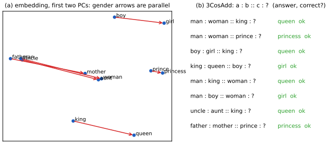
20.5.6 Contextual word embeddings
p. 712 A fixed embedding gives the same vector to "apple" in "I was eating an apple" and "I bought a new phone from Apple". Contextual embeddings make a word's vector a function of all the words in its context, usually the sentence (Section 15.7 of the book), and are the current standard preprocessing step for transfer learning (Section 19.2).
20.6 Exercises
All nine exercises of Chapter 20 (Murphy, 2022, pp. 712–714), restated in my own words, with complete solutions (hidden). A dagger marks the book's own flag for solutions available in its solution material; here every solution is worked independently. The notation of the notes is used throughout; \(\bm C\) in Exercises 20.3 to 20.5 is the sample covariance (written \(\bm S\) elsewhere in the notes).
Exercise 20.1 (EM for factor analysis). Derive the EM updates for the FA model \(\bm x=\bm W\bm z+\bm\epsilon\), \(\bm z\sim\N(\bm 0,\bm I)\), \(\bm\epsilon\sim\N(\bm 0,\bm\Psi)\) with diagonal \(\bm\Psi\). You may take \(\bm\mu=\bm 0\) as fixed.
Solution
With \(\bm\mu=\bm 0\), \(\log p(\bm x_i,\bm z_i)=-\frac12(\bm x_i-\bm W\bm z_i)^\T\bm\Psi^{-1}(\bm x_i-\bm W\bm z_i)-\frac12\log|\bm\Psi|-\frac12\|\bm z_i\|^2+\mathrm{const}\). E step. The posterior of \(\bm z_i\) has precision \(\bm I+\bm W^\T\bm\Psi^{-1}\bm W\) and linear term \(\bm W^\T\bm\Psi^{-1}\bm x_i\) (complete the square), so \(\bm z_i\given\bm x_i\sim\N(\bm m_i,\bm\Sigma)\) with \(\bm\Sigma=(\bm I+\bm W^\T\bm\Psi^{-1}\bm W)^{-1}\), \(\bm m_i=\bm\Sigma\bm W^\T\bm\Psi^{-1}\bm x_i\); and \(\E[\bm z_i\bm z_i^\T\given\bm x_i]=\bm\Sigma+\bm m_i\bm m_i^\T\). M step. \(Q=-\frac12\sum_i\{\bm x_i^\T\bm\Psi^{-1}\bm x_i-2\bm x_i^\T\bm\Psi^{-1}\bm W\bm m_i+\Tr(\bm W^\T\bm\Psi^{-1}\bm W(\bm\Sigma+\bm m_i\bm m_i^\T))\}-\frac N2\log|\bm\Psi|\). Setting \(\partial Q/\partial\bm W=\bm\Psi^{-1}[\sum_i\bm x_i\bm m_i^\T-\bm W\sum_i(\bm\Sigma+\bm m_i\bm m_i^\T)]=\bm 0\) gives \(\bm W^{\rm new}=\big(\sum_i\bm x_i\bm m_i^\T\big)\big(N\bm\Sigma+\sum_i\bm m_i\bm m_i^\T\big)^{-1}\). For the \(d\)th diagonal entry, \(\psi_d^{\rm new}=\frac1N\sum_i\E[(x_{id}-\bm w_d^\T\bm z_i)^2]=\frac1N[\sum_ix_{id}^2-2\bm w_d^\T\sum_i\bm m_ix_{id}+\bm w_d^\T(N\bm\Sigma+\sum_i\bm m_i\bm m_i^\T)\bm w_d]\), which by the \(\bm W\) equation equals \(\frac1N\sum_i(x_{id}-\bm w_d^\T\bm m_i)x_{id}\): \(\bm\Psi^{\rm new}=\frac1N\diag\{\sum_i(\bm x_i-\bm W^{\rm new}\bm m_i)\bm x_i^\T\}\). Details and the version with \(\bm\mu\) free are in Gap 20.8. Run on simulated data, the log likelihood increases at every iteration.
Exercise 20.2 (EM for a mixture of factor analysers) †. Derive the EM updates for a mixture of \(K\) factor analysers.
Solution
The complete data are \((m_n,\bm z_n,\bm x_n)\) with \(m_n\sim\mathrm{Cat}(\bm\pi)\), \(\bm z_n\sim\N(\bm 0,\bm I)\), \(\bm x_n\given m_n=k,\bm z_n\sim\N(\bm\mu_k+\bm W_k\bm z_n,\bm\Psi_k)\). E step. \(r_{nk}=p(m_n=k\given\bm x_n)\propto\pi_k\N(\bm x_n\given\bm\mu_k,\bm W_k\bm W_k^\T+\bm\Psi_k)\) (normalised over \(k\)); given \(m_n=k\), \(\bm z_n\given\bm x_n\sim\N(\bm m_{nk},\bm\Sigma_k)\), \(\bm\Sigma_k=(\bm I+\bm W_k^\T\bm\Psi_k^{-1}\bm W_k)^{-1}\), \(\bm m_{nk}=\bm\Sigma_k\bm W_k^\T\bm\Psi_k^{-1}(\bm x_n-\bm\mu_k)\). M step. \(Q=\sum_{n,k}r_{nk}[\log\pi_k+\E_{\bm z\sim\N(\bm m_{nk},\bm\Sigma_k)}\log\N(\bm x_n\given\bm\mu_k+\bm W_k\bm z,\bm\Psi_k)]+\mathrm{const}\). The \(\bm\pi\) terms give \(\pi_k=\frac1N\sum_nr_{nk}\). The terms in \((\bm\mu_k,\bm W_k,\bm\Psi_k)\) are the single-FA terms of Exercise 20.1 with datum \(n\) weighted by \(r_{nk}\): with \(\tilde{\bm W}_k=(\bm W_k,\bm\mu_k)\), \(\bm b_{nk}=(\bm m_{nk};1)\), \(\bm C_{nk}=\begin{pmatrix}\bm\Sigma_k+\bm m_{nk}\bm m_{nk}^\T&\bm m_{nk}\\\bm m_{nk}^\T&1\end{pmatrix}\), \[ \tilde{\bm W}_k^{\rm new}=\Big[\sum_nr_{nk}\bm x_n\bm b_{nk}^\T\Big]\Big[\sum_nr_{nk}\bm C_{nk}\Big]^{-1},\qquad\bm\Psi_k^{\rm new}=\frac{\diag\{\sum_nr_{nk}(\bm x_n-\tilde{\bm W}_k^{\rm new}\bm b_{nk})\bm x_n^\T\}}{\sum_nr_{nk}} . \] (Gap 20.11; for mixtures of PPCA with \(\bm\Psi_k=\sigma_k^2\bm I\) the M step can instead use the closed form of Gap 20.7 on the weighted covariance, which the code does: the log likelihood is non-decreasing and a single component reproduces PPCA.)
Exercise 20.3 (deriving the second principal component). (a) With \(J(\bm v_2,\bm z_2)=\frac1n\sum_i(\bm x_i-z_{i1}\bm v_1-z_{i2}\bm v_2)^\T(\bm x_i-z_{i1}\bm v_1-z_{i2}\bm v_2)\), show \(\partial J/\partial\bm z_2=\bm 0\) gives \(z_{i2}=\bm v_2^\T\bm x_i\). (b) Show that the \(\bm v_2\) minimising \(\tilde J(\bm v_2)=-\bm v_2^\T\bm C\bm v_2+\lambda_2(\bm v_2^\T\bm v_2-1)+\lambda_{12}(\bm v_2^\T\bm v_1-0)\) is the eigenvector of \(\bm C\) with the second largest eigenvalue. Hint: \(\bm C\bm v_1=\lambda_1\bm v_1\) and \(\partial\bm x^\T\bm A\bm x/\partial\bm x=(\bm A+\bm A^\T)\bm x\).
Solution
(a) \(\partial J/\partial z_{i2}=\frac1n[-2\bm v_2^\T(\bm x_i-z_{i1}\bm v_1-z_{i2}\bm v_2)]\), which vanishes when \(\bm v_2^\T\bm x_i-z_{i1}\bm v_2^\T\bm v_1-z_{i2}\bm v_2^\T\bm v_2=0\); with \(\bm v_2^\T\bm v_1=0\) and \(\bm v_2^\T\bm v_2=1\) this is \(z_{i2}=\bm v_2^\T\bm x_i\). (b) Substituting the optimal \(z_{i1}=\bm v_1^\T\bm x_i\), \(z_{i2}=\bm v_2^\T\bm x_i\) into \(J\) and using orthonormality gives \(J=\frac1n\sum_i[\bm x_i^\T\bm x_i-(\bm v_1^\T\bm x_i)^2-(\bm v_2^\T\bm x_i)^2]=\mathrm{const}-\bm v_2^\T\bm C\bm v_2\) (the terms in \(\bm v_1\) are fixed). The gradient of \(\tilde J\) is \(-2\bm C\bm v_2+2\lambda_2\bm v_2+\lambda_{12}\bm v_1=\bm 0\) (\(\bm C\) symmetric). Multiply by \(\bm v_1^\T\): \(-2\lambda_1\bm v_1^\T\bm v_2+2\lambda_2\bm v_1^\T\bm v_2+\lambda_{12}=\lambda_{12}=0\) because \(\bm v_1^\T\bm v_2=0\) and \(\bm v_1^\T\bm C=\lambda_1\bm v_1^\T\). So \(\bm C\bm v_2=\lambda_2\bm v_2\): a unit eigenvector orthogonal to \(\bm v_1\), with objective \(\bm v_2^\T\bm C\bm v_2=\lambda_2\) (the multiplier), to be maximised; among eigenvectors orthogonal to \(\bm v_1\) that is the one with the largest remaining eigenvalue, the second largest eigenvalue of \(\bm C\). (Gap 20.1 gives the global statement.) Numerically, scanning all unit vectors orthogonal to \(\bm v_1\) in three dimensions, the variance is maximal at the second eigenvector with value \(\lambda_2\) to \(10^{-9}\).
Exercise 20.4 (deriving the residual error of PCA) †. (a) For orthonormal \(\bm v_j\) and \(z_{ij}=\bm x_i^\T\bm v_j\), prove \(\|\bm x_i-\sum_{j=1}^Kz_{ij}\bm v_j\|^2=\bm x_i^\T\bm x_i-\sum_{j=1}^K\bm v_j^\T\bm x_i\bm x_i^\T\bm v_j\). (b) Show \(J_K=\frac1n\sum_i\big(\bm x_i^\T\bm x_i-\sum_{j\le K}\bm v_j^\T\bm x_i\bm x_i^\T\bm v_j\big)=\frac1n\sum_i\bm x_i^\T\bm x_i-\sum_{j\le K}\lambda_j\). (c) With \(J_d=0\) for \(K=d\), show \(J_K=\sum_{j=K+1}^d\lambda_j\).
Solution
(a) Expand: \(\|\bm x-\sum_jz_j\bm v_j\|^2=\bm x^\T\bm x-2\sum_jz_j\bm v_j^\T\bm x+\sum_{j,k}z_jz_k\bm v_j^\T\bm v_k=\bm x^\T\bm x-2\sum_jz_j^2+\sum_jz_j^2=\bm x^\T\bm x-\sum_jz_j^2\) using \(\bm v_j^\T\bm x=z_j\), \(\bm v_j^\T\bm v_k=\delta_{jk}\), and \(z_j^2=\bm v_j^\T\bm x\bm x^\T\bm v_j\). (b) Average and use \(\frac1n\sum_i\bm x_i\bm x_i^\T=\bm C\) (centred data): \(J_K=\frac1n\sum_i\bm x_i^\T\bm x_i-\sum_{j\le K}\bm v_j^\T\bm C\bm v_j\), and \(\bm v_j^\T\bm C\bm v_j=\lambda_j\bm v_j^\T\bm v_j=\lambda_j\) for eigenvectors. (c) For \(K=d\) the vectors \(\bm v_1,\dots,\bm v_d\) form an orthonormal basis, so the reconstruction is exact and \(J_d=0\): \(\frac1n\sum_i\bm x_i^\T\bm x_i=\sum_{j\le d}\lambda_j\) (equivalently \(\Tr\bm C\)). Then \(J_K=\sum_{j\le d}\lambda_j-\sum_{j\le K}\lambda_j=\sum_{j=K+1}^d\lambda_j\), (20.26). (Gap 20.1, Step 3.)
Exercise 20.5 (PCA via successive deflation). Let \(\bm v_1,\bm v_2,\dots\) be the principal eigenvectors of \(\bm C=\frac1n\bm X^\T\bm X\) with \(\bm v_j^\T\bm v_k=\delta_{jk}\). Define the deflated data \(\tilde{\bm x}_i=(\bm I-\bm v_1\bm v_1^\T)\bm x_i\) and \(\tilde{\bm X}=(\bm I-\bm v_1\bm v_1^\T)\bm X\) (as written, with the matrix acting on the transposed data). (a) Using \(\bm X^\T\bm X\bm v_1=n\lambda_1\bm v_1\), show that \(\tilde{\bm C}=\frac1n\tilde{\bm X}^\T\tilde{\bm X}=\frac1n\bm X^\T\bm X-\lambda_1\bm v_1\bm v_1^\T\). (b) Let \(\bm u\) be the principal eigenvector of \(\tilde{\bm C}\); explain why \(\bm u=\bm v_2\). (c) Given a routine \([\lambda,\bm u]=f(\bm C)\) returning the leading eigenpair of a positive definite matrix, write pseudo-code for the first \(K\) principal basis vectors using only \(f\) and vector arithmetic.
Solution
(With rows as data points, the deflated data matrix is \(\tilde{\bm X}=\bm X(\bm I-\bm v_1\bm v_1^\T)\); the exercise's expression is the same thing for \(\bm X\) with data in columns.) Let \(\bm P=\bm I-\bm v_1\bm v_1^\T\), a symmetric projector, \(\bm P^2=\bm P\). (a) \(\tilde{\bm C}=\frac1n\bm P\bm X^\T\bm X\bm P=\bm P\bm C\bm P\) with \(\bm C=\frac1n\bm X^\T\bm X\), and \(\bm C\bm v_1=\lambda_1\bm v_1\) gives \(\bm P\bm C\bm P=\bm C-\bm v_1\bm v_1^\T\bm C-\bm C\bm v_1\bm v_1^\T+\bm v_1\bm v_1^\T\bm C\bm v_1\bm v_1^\T=\bm C-\lambda_1\bm v_1\bm v_1^\T-\lambda_1\bm v_1\bm v_1^\T+\lambda_1\bm v_1\bm v_1^\T=\bm C-\lambda_1\bm v_1\bm v_1^\T\), as claimed. (b) With \(\bm C=\sum_j\lambda_j\bm v_j\bm v_j^\T\), \(\tilde{\bm C}=\sum_{j\ge2}\lambda_j\bm v_j\bm v_j^\T\): the eigenvectors are those of \(\bm C\), with \(\bm v_1\) now belonging to eigenvalue 0 and the others unchanged. The largest eigenvalue of \(\tilde{\bm C}\) is therefore \(\lambda_2\) (as \(\lambda_2\ge\lambda_3\ge\dots\ge0\)), with eigenvector \(\bm v_2\) (unique up to sign when \(\lambda_2>\lambda_3\)). (c) Pseudo-code:
for k = 1..K: [lambda_k, v_k] = f(C); C = C - lambda_k * outer(v_k, v_k); the output is \(\{\lambda_k,\bm v_k\}\) (by induction each step removes the previous eigencomponent). I implemented \(f\) as power iteration (2000 steps from a fixed start) and ran this on the digit data: the first four eigenvalues and eigenvectors agree with the direct eigendecomposition to \(10^{-6}\). Remarks: errors in \(\bm v_k\) propagate through the deflation, so for many components orthogonalisation against the earlier vectors is advisable, and power iteration's speed depends on \(\lambda_{k+1}/\lambda_k\) as in Gap 20.9.Exercise 20.6 (PPCA variance terms). In PPCA, \(\bm C=\bm W\bm W^\T+\sigma^2\bm I\). Show that the model correctly captures the variance along the principal axes and approximates it by \(\sigma^2\) in all other directions. For a unit vector \(\bm v\) the predictive variance along \(\bm v\) is \(\bm v^\T\bm C\bm v\). (a) If \(\bm v\) is orthogonal to the principal subspace (\(\bm v^\T\bm U=\bm 0\)), show \(\bm v^\T\bm C\bm v=\sigma^2\). (b) If \(\bm v=\bm u_i\) is a principal eigenvector, show \(\bm v^\T\bm C\bm v=(\lambda_i-\sigma^2)+\sigma^2=\lambda_i\).
Solution
With the maximum likelihood \(\bm W=\bm U_L(\bm\Lambda_L-\sigma^2\bm I)^{1/2}\) (take \(\bm R=\bm I\)), \(\bm v^\T\bm C\bm v=\|\bm W^\T\bm v\|^2+\sigma^2\|\bm v\|^2=\|\bm W^\T\bm v\|^2+\sigma^2\). (a) \(\bm W^\T\bm v=(\bm\Lambda_L-\sigma^2\bm I)^{1/2}\bm U_L^\T\bm v=\bm 0\), so \(\bm v^\T\bm C\bm v=\sigma^2\). (b) \(\bm U_L^\T\bm u_i=\bm e_i\), so \(\bm W^\T\bm u_i=(\lambda_i-\sigma^2)^{1/2}\bm e_i\) and \(\bm v^\T\bm C\bm v=(\lambda_i-\sigma^2)+\sigma^2=\lambda_i\) (this needs \(\lambda_i\ge\sigma^2\), which holds since \(\sigma^2\) is the mean of eigenvalues not larger than \(\lambda_{L+1}\le\lambda_i\)). Hence the model reproduces the empirical variance exactly along each retained principal axis, and spreads the remaining variance evenly (\(\sigma^2\) is the average of the discarded eigenvalues) over the orthogonal complement. See Gap 20.7, which also proves that the choice is the global maximum of the likelihood.
Exercise 20.7 (posterior inference in PPCA) †. Derive \(p(\bm z_n\given\bm x_n)\) for the PPCA model.
Solution
\(p(\bm z\given\bm x)\propto\N(\bm z\given\bm 0,\bm I)\N(\bm x\given\bm W\bm z+\bm\mu,\sigma^2\bm I)\), so \(\log p(\bm z\given\bm x)=-\frac12\bm z^\T\bm z-\frac1{2\sigma^2}\|\bm x-\bm\mu-\bm W\bm z\|^2+\mathrm{const}=-\frac12\bm z^\T\big(\bm I+\sigma^{-2}\bm W^\T\bm W\big)\bm z+\sigma^{-2}\bm z^\T\bm W^\T(\bm x-\bm\mu)+\mathrm{const}\). With \(\bm M=\bm W^\T\bm W+\sigma^2\bm I\), the precision is \(\sigma^{-2}\bm M\) and the linear term \(\sigma^{-2}\bm W^\T(\bm x-\bm\mu)\): the posterior is Gaussian with covariance \(\sigma^2\bm M^{-1}\) and mean \(\sigma^2\bm M^{-1}\cdot\sigma^{-2}\bm W^\T(\bm x-\bm\mu)=\bm M^{-1}\bm W^\T(\bm x-\bm\mu)\) (20.52). Check against Gap 20.6: \(\bm W^\T\bm C^{-1}=\bm M^{-1}\bm W^\T\) and \(\bm I-\bm W^\T\bm C^{-1}\bm W=\sigma^2\bm M^{-1}\), confirmed numerically; as \(\sigma^2\to0\) the mean tends to \((\bm W^\T\bm W)^{-1}\bm W^\T(\bm x-\bm\mu)\), (20.53).
Exercise 20.8 (imputation in an FA model) †. For an FA model with data \(\bm x=(\bm x_h,\bm x_v)\) partitioned into hidden and visible parts, derive \(p(\bm x_h\given\bm x_v,\bm\theta)\).
Solution
\(\bm x\sim\N(\bm\mu,\bm C)\), \(\bm C=\bm W\bm W^\T+\bm\Psi\); partition \(\bm W=\begin{pmatrix}\bm W_h\\\bm W_v\end{pmatrix}\), \(\bm\Psi=\diag(\bm\Psi_h,\bm\Psi_v)\) (diagonal, so no coupling), so \(\bm C_{hh}=\bm W_h\bm W_h^\T+\bm\Psi_h\), \(\bm C_{hv}=\bm W_h\bm W_v^\T\), \(\bm C_{vv}=\bm W_v\bm W_v^\T+\bm\Psi_v\). By Gaussian conditioning (Section 3.2.3), \[ p(\bm x_h\given\bm x_v)=\N\big(\bm x_h\given\bm\mu_h+\bm C_{hv}\bm C_{vv}^{-1}(\bm x_v-\bm\mu_v),\ \bm C_{hh}-\bm C_{hv}\bm C_{vv}^{-1}\bm C_{vh}\big) . \] An equivalent route that avoids the \(|v|\times|v|\) inverse: the posterior of \(\bm z\) given only the visible coordinates is \(\N(\bm m_v,\bm\Sigma_v)\) with \(\bm\Sigma_v=(\bm I+\bm W_v^\T\bm\Psi_v^{-1}\bm W_v)^{-1}\), \(\bm m_v=\bm\Sigma_v\bm W_v^\T\bm\Psi_v^{-1}(\bm x_v-\bm\mu_v)\) (Gap 20.6 restricted to the visible rows); since \(\bm x_h=\bm\mu_h+\bm W_h\bm z+\bm\epsilon_h\) with \(\bm\epsilon_h\) independent of \(\bm x_v\) given \(\bm z\), \[ p(\bm x_h\given\bm x_v)=\N\big(\bm x_h\given\bm\mu_h+\bm W_h\bm m_v,\ \bm W_h\bm\Sigma_v\bm W_h^\T+\bm\Psi_h\big) . \] The two expressions agree (checked numerically for a model with \(D=6\), \(L=2\), two hidden and four visible coordinates, to \(10^{-10}\)); this is what the E step of EM with missing data computes.
Exercise 20.9 (efficiently evaluating the PPCA density). Derive an expression for \(p(\bm x\given\hat{\bm W},\hat\sigma^2)\) of the PPCA model by plugging in the maximum likelihood estimates and using the matrix inversion lemma.
Solution
At the maximum, \(\hat{\bm W}=\bm U_L(\bm\Lambda_L-\hat\sigma^2\bm I)^{1/2}\) and \(\bm C=\hat{\bm W}\hat{\bm W}^\T+\hat\sigma^2\bm I\). The matrix inversion lemma (Gap 20.7) with \(\bm M=\hat{\bm W}^\T\hat{\bm W}+\hat\sigma^2\bm I=\bm\Lambda_L\) gives \(\bm C^{-1}=\hat\sigma^{-2}\big(\bm I-\bm U_L(\bm\Lambda_L-\hat\sigma^2\bm I)\bm\Lambda_L^{-1}\bm U_L^\T\big)\) and \(\log|\bm C|=(D-L)\log\hat\sigma^2+\sum_{j\le L}\log\lambda_j\). With \(\bm c=\bm x-\hat{\bm\mu}\) and \(a_j=\bm u_j^\T\bm c\), \[ \log p(\bm x)=-\frac12\Big[D\log2\pi+\sum_{j=1}^L\log\lambda_j+(D-L)\log\hat\sigma^2+\frac1{\hat\sigma^2}\Big(\|\bm c\|^2-\sum_{j=1}^L\frac{\lambda_j-\hat\sigma^2}{\lambda_j}a_j^2\Big)\Big] , \] using \(\bm c^\T\bm C^{-1}\bm c=\hat\sigma^{-2}[\|\bm c\|^2-\sum_j(1-\hat\sigma^2/\lambda_j)a_j^2]\). The cost is \(O(DL)\) per point and no matrix inversion; as \(L\) sums only the retained eigenpairs, the discarded ones enter only through \(\hat\sigma^2\). I verified that this formula equals the direct evaluation of the Gaussian density with \(\bm C=\hat{\bm W}\hat{\bm W}^\T+\hat\sigma^2\bm I\).
Demonstrations
| Page | What it shows | In the notes |
|---|---|---|
| PCA reconstruction, scree plot and profile likelihood | PCA on 600 handwritten digits (8 × 8) with 400 held out and optional pixel noise: six digits clean, noisy and reconstructed from \(L\) components; training, held-out and clean-target error against \(L\); the scree plot; the profile likelihood and its \(L^*\). Presets: 1 clean digits, no U shape; 2 noise 4, best \(L\); 3 heavy noise; 4 two components; 5 too many components. | 20.1.4, gap 20.4, gap 20.5 |
| EM for PCA and probabilistic PCA | The rod and the springs: step through E and M steps on 2-D data with one latent dimension, with and without a learned noise variance; the angle to the first axis and the objective against the sweep; the convergence rate \(\lambda_2/\lambda_1\). Presets: 1 far start; 2 slow, eigenvalue ratio 0.8; 3 PPCA, learned \(\sigma^2\); 4 height and weight; 5 height and weight, PPCA. | 20.2.2, 20.2.3, gap 20.7, gap 20.9 |
| t-SNE: perplexity and the crowding problem | t-SNE and Gaussian symmetric SNE implemented in the page: perplexity slider, gradient descent with early exaggeration, the KL curve, on three clusters, 300 digits and a Swiss roll. Presets: 1 perplexity 5 shatters clusters; 2 perplexity 30; 3 digits; 4 digits with the Gaussian kernel (crowding); 5 Swiss roll. | 20.4.10, gap 20.24, gap 20.25 |
| Isomap and short circuits | A 500-point Swiss roll: Isomap against classical MDS, the number of neighbours \(K\) and the noise; the neighbourhood graph with short-circuit edges in red, the connected components, the unrolling score. Presets: 1 \(K=6\) unrolls; 2 \(K=14\) folds; 3 \(K=30\); 4 noisy roll; 5 classical MDS. | 20.4.4, 20.4.5, gap 20.18, gap 20.19 |
The Python code that produces every figure of this page is code/ch20_dimensionality_reduction.py (see the code index). Companion demos: PCA and probabilistic PCA, kernel PCA, Bayesian PCA, VAE latent explorer.
Notes on the book
Points where the book is imprecise or wrong
- (20.36), the reduction \(\tilde{\bm W}=\bm W\bm\Sigma_0^{-1/2}\). Absorbing a correlated prior \(\N(\bm 0,\bm\Sigma_0)\) needs \(\tilde{\bm W}=\bm W\bm\Sigma_0^{1/2}\); with the exponent \(-\frac12\) the covariance would be \(\bm W\bm\Sigma_0^{-1}\bm W^\T\) (gap 20.6).
- (20.49). The expression \(\bm U_L(\bm\Lambda_L-\sigma^2\bm I)\bm U_L^\T+\sigma^2\bm I\) is the \(D\times D\) covariance \(\bm C\) at the maximum, not the \(L\times L\) matrix \(\bm M=\bm W^\T\bm W+\sigma^2\bm I\) of (20.48), which equals \(\bm\Lambda_L\) there (gap 20.7).
- (20.72). The marginal of the mixture of factor analysers is written with \(\N(\bm z\given\bm\mu_k,\bm I)\) and \(\N(\bm x\given\bm W\bm z,\sigma^2\bm I)\), which does not match (20.69)–(20.71): the prior of \(\bm z\) has mean \(\bm 0\), and the likelihood has mean \(\bm\mu_k+\bm W_k\bm z\) and covariance \(\bm\Psi_k\) (gap 20.11).
- Denoising autoencoders: the score. The residual of a DAE trained with Gaussian noise of variance \(\sigma^2\) tends to \(\sigma^2\nabla\log p\), not \(\nabla\log p\), and in Alain and Bengio it is measured from the corrupted input, \(r(\tilde{\bm x})-\tilde{\bm x}\), not from the clean \(\bm x\) (gap 20.15).
- (20.95). The Bernoulli likelihood is printed as \(\mathrm{Ber}(x_i\given f_d(\bm z;\bm\theta),\sigma^2\bm I)\); a Bernoulli has no variance parameter (Section 20.3.5).
- (20.116). The constraint \(\bm K\succ0\) should be \(\bm K\succeq0\): the Gram matrix of a low-dimensional embedding of \(N\) points is singular (gap 20.21).
- (20.119). The LLE embedding problem as written has the trivial solution \(\bm Z=\bm 0\); it needs the constraints \(\bm 1^\T\bm Z=\bm 0\) and \(\frac1N\bm Z^\T\bm Z=\bm I\), which are implicit in the choice of eigenvectors of the smallest nonzero eigenvalues (gap 20.22).
- (20.134)–(20.138), normalisation of the SNE probabilities. (20.134) sums over \(i<j\), (20.135) normalises over \(k\ne l\) and (20.137) over \(k<l\). The factor 4 in the gradients (20.136), (20.138) holds when pairs are counted in both orders and \(\sum_{i\ne j}p_{ij}=1\); with unordered pairs normalised to 1 the same gradient is written with the factor 2 (gap 20.24).
- (20.156). The GloVe objective is printed with a leading minus sign in front of a sum of weighted squares; it must be a plus (gap 20.27).
- (20.159). The PMI is printed without the logarithm; with the definition (20.143) the RAND-WALK result is \(\log\frac{p(w,w')}{p(w)p(w')}\approx\bm v_w^\T\bm v_{w'}/D\) (gap 20.28).
- Exercise 20.5, dimensions. \(\tilde{\bm X}=(\bm I-\bm v_1\bm v_1^\T)^\T\bm X\) is only dimensionally consistent if the data are the columns of \(\bm X\), but the covariance is defined as \(\frac1n\bm X^\T\bm X\), which requires rows. With data in rows the deflated matrix is \(\bm X(\bm I-\bm v_1\bm v_1^\T)\) (Exercise 20.5).
- Section 20.1.4.1, the cause of the missing U shape. The book attributes the monotone test error to PCA not being a proper generative model. The monotonicity is a property of any orthogonal projection (the error of every point decreases with each added direction, gap 20.4); a proper generative model, PPCA, can overfit in the held-out likelihood, though in the digits experiment this appeared only close to full rank.
- Section 20.4.2. The rotated-image family is parametrised by one angle, so its intrinsic dimension is 1; the plane in which it is drawn (Figure 20.29c) is two-dimensional (Section 20.4.2).
References
- Murphy, K. P. (2022). Probabilistic Machine Learning: An Introduction. MIT Press, Cambridge, MA. Chapter 20, pp. 657–714. probml.github.io/pml-book/book1.html.
- Alain, G. and Bengio, Y. (2014). What regularized auto-encoders learn from the data-generating distribution. Journal of Machine Learning Research, 15, 3563–3593.
- Allen, C. and Hospedales, T. (2019). Analogies explained: towards understanding word embeddings. International Conference on Machine Learning.
- Andreas, J. and Klein, D. (2015). When and why are log-linear models self-normalizing? NAACL.
- Anowar, F., Sadaoui, S. and Selim, B. (2021). Conceptual and empirical comparison of dimensionality reduction algorithms (PCA, KPCA, LDA, MDS, SVD, LLE, ISOMAP, LE, ICA, t-SNE). Computer Science Review, 40, 100378.
- Arora, S., Li, Y., Liang, Y., Ma, T. and Risteski, A. (2016). A latent variable model approach to PMI-based word embeddings. Transactions of the Association for Computational Linguistics, 4, 385–399.
- Bach, F. R. and Jordan, M. I. (2005). A probabilistic interpretation of canonical correlation analysis. Technical Report 688, Department of Statistics, University of California, Berkeley.
- Baldi, P. and Hornik, K. (1989). Neural networks and principal component analysis: learning from examples without local minima. Neural Networks, 2(1), 53–58.
- Balasubramanian, M. and Schwartz, E. L. (2002). The Isomap algorithm and topological stability. Science, 295, 7.
- Barnes, J. and Hut, P. (1986). A hierarchical \(O(N\log N)\) force-calculation algorithm. Nature, 324, 446–449.
- Belkin, M. and Niyogi, P. (2001). Laplacian eigenmaps and spectral techniques for embedding and clustering. Advances in Neural Information Processing Systems, 14.
- Belkin, M. and Niyogi, P. (2003). Laplacian eigenmaps for dimensionality reduction and data representation. Neural Computation, 15(6), 1373–1396.
- Bengio, Y., Paiement, J.-F., Vincent, P., Delalleau, O., Le Roux, N. and Ouimet, M. (2004). Out-of-sample extensions for LLE, Isomap, MDS, eigenmaps, and spectral clustering. Advances in Neural Information Processing Systems, 16.
- Bernstein, M., de Silva, V., Langford, J. C. and Tenenbaum, J. B. (2000). Graph approximations to geodesics on embedded manifolds. Technical report, Stanford University.
- Bishop, C. M. (1995). Training with noise is equivalent to Tikhonov regularization. Neural Computation, 7(1), 108–116.
- Bullinaria, J. A. and Levy, J. P. (2007). Extracting semantic representations from word co-occurrence statistics: a computational study. Behavior Research Methods, 39(3), 510–526.
- Choi, H. and Choi, S. (2007). Robust kernel Isomap. Pattern Recognition, 40(3), 853–862.
- Coenen, A. and Pearce, A. (2019). Understanding UMAP. Google PAIR (online article).
- Collins, M., Dasgupta, S. and Schapire, R. E. (2002). A generalization of principal components analysis to the exponential family. Advances in Neural Information Processing Systems, 14.
- Davis, C. (1990). Body image and weight preoccupation: a comparison between exercising and non-exercising women. Appetite, 15, 13–21.
- Dayan, P., Hinton, G. E., Neal, R. M. and Zemel, R. S. (1995). The Helmholtz machine. Neural Computation, 7(5), 889–904.
- Deerwester, S., Dumais, S. T., Furnas, G. W., Landauer, T. K. and Harshman, R. (1990). Indexing by latent semantic analysis. Journal of the American Society for Information Science, 41(6), 391–407.
- Eisenstein, J. (2019). Introduction to Natural Language Processing. MIT Press, Cambridge, MA.
- Ethayarajh, K., Duvenaud, D. and Hirst, G. (2019). Towards understanding linear word analogies. Annual Meeting of the Association for Computational Linguistics.
- Firth, J. R. (1957). A synopsis of linguistic theory, 1930–1955. In Studies in Linguistic Analysis, Blackwell, Oxford.
- Glorot, X., Bordes, A. and Bengio, Y. (2011). Deep sparse rectifier neural networks. International Conference on Artificial Intelligence and Statistics.
- Harris, Z. S. (1954). Distributional structure. Word, 10(2–3), 146–162.
- Hinton, G. E. and Roweis, S. T. (2003). Stochastic neighbor embedding. Advances in Neural Information Processing Systems, 15.
- Hotelling, H. (1936). Relations between two sets of variates. Biometrika, 28(3–4), 321–377.
- Jaakkola, T. S. and Jordan, M. I. (2000). Bayesian parameter estimation via variational methods. Statistics and Computing, 10(1), 25–37.
- Japkowicz, N., Hanson, S. J. and Gluck, M. A. (2000). Nonlinear autoassociation is not equivalent to PCA. Neural Computation, 12(3), 531–545.
- Kaiser, H. F. (1958). The varimax criterion for analytic rotation in factor analysis. Psychometrika, 23(3), 187–200.
- Karhunen, J. and Joutsensalo, J. (1995). Generalizations of principal component analysis, optimization problems, and neural networks. Neural Networks, 8(4), 549–562.
- Khan, M. E., Bouchard, G., Murphy, K. P. and Marlin, B. M. (2010). Variational bounds for mixed-data factor analysis. Advances in Neural Information Processing Systems, 23.
- Kingma, D. P. and Welling, M. (2014). Auto-encoding variational Bayes. International Conference on Learning Representations.
- Ledermann, W. (1937). On the rank of the reduced correlational matrix in multiple-factor analysis. Psychometrika, 2(2), 85–93.
- de Leeuw, J. (1977). Applications of convex analysis to multidimensional scaling. In Recent Developments in Statistics, North-Holland, Amsterdam.
- Levy, O. and Goldberg, Y. (2014). Neural word embedding as implicit matrix factorization. Advances in Neural Information Processing Systems, 27.
- Lucas, J., Tucker, G., Grosse, R. and Norouzi, M. (2019). Don't blame the ELBO! A linear VAE perspective on posterior collapse. Advances in Neural Information Processing Systems, 32.
- van der Maaten, L. (2014). Accelerating t-SNE using tree-based algorithms. Journal of Machine Learning Research, 15, 3221–3245.
- van der Maaten, L. and Hinton, G. (2008). Visualizing data using t-SNE. Journal of Machine Learning Research, 9, 2579–2605.
- McInnes, L., Healy, J. and Melville, J. (2018). UMAP: uniform manifold approximation and projection for dimension reduction. arXiv:1802.03426.
- Mikolov, T., Chen, K., Corrado, G. and Dean, J. (2013a). Efficient estimation of word representations in vector space. arXiv:1301.3781.
- Mikolov, T., Sutskever, I., Chen, K., Corrado, G. and Dean, J. (2013b). Distributed representations of words and phrases and their compositionality. Advances in Neural Information Processing Systems, 26.
- Miyasawa, K. (1961). An empirical Bayes estimator of the mean of a normal population. Bulletin of the International Statistical Institute, 38, 181–188.
- Pennington, J., Socher, R. and Manning, C. D. (2014). GloVe: global vectors for word representation. Empirical Methods in Natural Language Processing.
- Rezende, D. J., Mohamed, S. and Wierstra, D. (2014). Stochastic backpropagation and approximate inference in deep generative models. International Conference on Machine Learning.
- Rifai, S., Vincent, P., Muller, X., Glorot, X. and Bengio, Y. (2011). Contractive auto-encoders: explicit invariance during feature extraction. International Conference on Machine Learning.
- Robbins, H. (1956). An empirical Bayes approach to statistics. Proceedings of the Third Berkeley Symposium on Mathematical Statistics and Probability, 1, 157–163.
- Roweis, S. T. (1997). EM algorithms for PCA and SPCA. Advances in Neural Information Processing Systems, 10.
- Roweis, S. T. and Saul, L. K. (2000). Nonlinear dimensionality reduction by locally linear embedding. Science, 290, 2323–2326.
- Schölkopf, B., Smola, A. and Müller, K.-R. (1998). Nonlinear component analysis as a kernel eigenvalue problem. Neural Computation, 10(5), 1299–1319.
- Shao, H., Kumar, A. and Fletcher, P. T. (2018). The Riemannian geometry of deep generative models. CVPR Workshops.
- Tenenbaum, J. B., de Silva, V. and Langford, J. C. (2000). A global geometric framework for nonlinear dimensionality reduction. Science, 290, 2319–2323.
- Tipping, M. E. (1998). Probabilistic visualisation of high-dimensional binary data. Advances in Neural Information Processing Systems, 11.
- Tipping, M. E. and Bishop, C. M. (1999). Probabilistic principal component analysis. Journal of the Royal Statistical Society, Series B, 61(3), 611–622.
- Vincent, P., Larochelle, H., Lajoie, I., Bengio, Y. and Manzagol, P.-A. (2010). Stacked denoising autoencoders. Journal of Machine Learning Research, 11, 3371–3408.
- Wattenberg, M., Viégas, F. and Johnson, I. (2016). How to use t-SNE effectively. Distill.
- Weinberger, K. Q., Sha, F. and Saul, L. K. (2004). Learning a kernel matrix for nonlinear dimensionality reduction. International Conference on Machine Learning.
- Yu, S., Yu, K., Tresp, V., Kriegel, H.-P. and Wu, M. (2006). Supervised probabilistic principal component analysis. Knowledge Discovery and Data Mining.
- Zhao, J.-H. and Yu, P. L. H. (2008). Fast ML estimation for the mixture of factor analyzers via an ECM algorithm. IEEE Transactions on Neural Networks, 19(11), 1956–1961.
- Zhu, M. and Ghodsi, A. (2006). Automatic dimensionality selection from the scree plot via the use of profile likelihood. Computational Statistics and Data Analysis, 51(2), 918–930.
The numerical statements in the text (the equivalence of the eigenvector, SVD and Gram-matrix routes to PCA, the error identity and the monotone test error, the scale dependence of covariance PCA, the profile likelihood and its closed form, the FA marginal and posterior, the PPCA maximum and its efficient formulas, EM for FA and for PCA with its rate, the parameter count of FA, supervised PCA and CCA, the linear autoencoder, Tweedie's identity, the contractive penalty, the ELBO identities, the reparameterisation gradient, classical MDS as PCA, SMACOF, Isomap, kernel PCA with test-point centring, LLE, the Laplacian, the SNE, symmetric SNE and t-SNE gradients, the perplexity search, the shifted-PMI optimum of skip-gram and the parallelogram rule) were confirmed numerically, and the reference numbers of the demonstration pages were reproduced.