Probability
Probability is the language in which all of statistical inference is written, so this chapter fixes its grammar. Outcomes of an experiment form a sample space, questions about the outcome are events, and a probability is a function on events obeying three axioms. Everything else, from the rule for the probability of a union to Bayes' theorem, is derived from those axioms. The derivations are short but they are where the subtleties live: countable additivity is what makes probabilities continuous along increasing and decreasing sequences of events (and what makes long-run frequencies converge), independence of several events is more than independence of each pair, conditioning on an event is renormalising the probability inside it, and the base rate of a condition can matter more than the accuracy of the test that detects it. The appendix explains why, on an uncountable sample space, probabilities can only be assigned to the events of a σ-field.
Ch. 1 Probability Ch. 2 Random variables Ch. 3 Expectation Ch. 4 Inequalities Ch. 5 Convergence Ch. 6 Models and inference Ch. 7 Estimating the CDF Ch. 8 Bootstrap Ch. 9 Parametric inference Ch. 10 Hypothesis testing Ch. 11 Bayesian inference Ch. 12 Decision theory Ch. 13 Regression Ch. 14 Multivariate models Ch. 15 Independence Ch. 16 Causal inference Ch. 17 Directed graphs Ch. 18 Undirected graphs Ch. 19 Log-linear models Ch. 20 Curve estimation Ch. 21 Orthogonal functions Ch. 22 Classification Ch. 23 Stochastic processes Ch. 24 Simulation
How to read these notes
They follow the book. Sections carry the book's numbers (1.1 to 1.10). Definitions, lemmas, theorems, examples and exercises keep the book's numbers (Definition 1.5, Lemma 1.6, Theorem 1.8, ...), and displayed equations that the book numbers keep their number, e.g. \((1.4)\). Results and definitions that these notes add are lettered (Definition 1.A, Result 1.B, ...), so a number always refers to the book.
Filling the gaps. Wherever the book states a fact without proof, says that "it can be shown", or leaves a step to an exercise, an orange Filling the gap box or a proof gives a complete argument. Proofs and derivations start hidden: open one with its bar, or use the button below.
Figures and demonstrations. The chapter has no figures of its own; the eight supplementary figures (numbered 1.S1 to 1.S8) are computed by the Python code for the examples and the computer experiments of the exercises. The ▶ Demo boxes open an interactive demonstration already set to the case being discussed.
Main reference
L. Wasserman, All of Statistics: A Concise Course in Statistical Inference, Springer (2004), Chapter 1, pages 3–17 (book website, with the data sets and the author's errata: www.stat.cmu.edu/~larry/all-of-statistics). Section, equation, example, figure and exercise numbers below refer to this book. Further reading is listed in the references.
The explanations, derivations, figures and code are my own; results and equations are cited by their numbers in the book.
Companion courses
The rules of probability are also the starting point of three other courses on this site. The overlapping material is:
- Bayesian and Probabilistic Machine Learning, Chapter 1, Section 1.2 (probability theory): the sum and product rules and Bayes' theorem (Definition 1.2, with the worked boxes of fruit) and the Bayesian reading of probability as a degree of belief (Section 1.2.3).
- Foundations of Deep Learning, Chapter 2, Section 2.1 (the rules of probability): the medical screening example (2.1.1, 2.1.4), Bayes' theorem (2.1.3) in odds form with repeated tests (Filling the gap 2.1), and independence (2.1.6); its screening demo complements the Bayes demo here.
- The first-year notes Estimation and Hypothesis Testing (advanced version), Section 0.1 (the axioms, with Proposition 0.1 on complements, monotonicity and the union of two events) and Section 0.3 (Chebyshev's inequality and the weak law of large numbers).
Those courses work with the sum and product rules for random variables and do not need the measure-theoretic side. New here: the consequences of countable additivity (continuity, Boole's inequality, the Borel–Cantelli lemma and a strong law for coin tossing), inclusion–exclusion with the Bonferroni inequalities, the difference between pairwise and mutual independence, the Monty Hall problem on its sample space, and the appendix on σ-fields (Vitali's non-measurable set and the uniqueness of probability measures).
The chapter at a glance
- 1.2 Outcomes form a sample space \(\Omega\); events are subsets of \(\Omega\), combined with the set operations. A sequence of events has a limit when its lim sup and lim inf agree (Definition 1.A).
- 1.3 A probability is nonnegative, gives \(\Omega\) probability 1 and is countably additive (Definition 1.5). From this: the rules (1.1) (Result 1.B), inclusion–exclusion (Lemma 1.6, Result 1.C), Boole's inequality (Result 1.D), and continuity along convergent sequences of events (Theorem 1.8), which is equivalent to countable additivity (Result 1.E).
- 1.4 With finitely many equally likely outcomes, probability is counting (Result 1.F).
- 1.5 Independence of a family of events means a product rule for every finite sub-family (Definition 1.9); pairwise independence is weaker (Result 1.G). With continuity, independence gives the Borel–Cantelli lemma and the convergence of long-run frequencies (Result 1.H).
- 1.6 Conditioning on \(B\) renormalises \(\P\) inside \(B\) and is again a probability (Definition 1.12, Result 1.J, Lemma 1.14); \(\P(A\given B)\) and \(\P(B\given A)\) are different numbers.
- 1.7 The law of total probability and Bayes' theorem (Theorems 1.16 and 1.17); the posterior depends on the base rate as much as on the accuracy of the evidence (Filling the gap 1.11).
- 1.9 \(\sigma\)-fields (Definition 1.K): no countably additive, translation-invariant probability exists on all subsets of \([0,1)\) (Result 1.L), and a probability is determined by its values on intervals (Result 1.M).
Notation. \(\Omega\) is the sample space, \(\omega\) an outcome, \(A,B,C\) events, \(A^c\) the complement, \(AB=A\cap B\), \(|A|\) the number of elements of a finite set, \(I_A\) the indicator function of \(A\). \(\P\) is a probability, \(\cA\) a \(\sigma\)-field. \(A_n\uparrow A\) and \(A_n\downarrow A\) denote increasing and decreasing sequences with limit \(A\).
Prerequisites. Sets and functions, sequences and series of real numbers (in particular, series of nonnegative terms may be summed in any order), and countable and uncountable sets. No measure theory is assumed; the little that is needed is developed in Section 1.9.
1.1 Introduction
p. 3 Probability is a mathematical language for uncertainty. Its objects are few: the set of possible outcomes of an experiment, the events we may ask about, and a function assigning each event a number between 0 and 1. The book introduces them in this order, derives the rules every probability calculation uses, and then turns to the two ideas that do most of the work in statistics: independence and conditioning.
1.2 Sample Spaces and Events
pp. 3–5 The sample space \(\Omega\) is the set of possible outcomes of an experiment; its elements \(\omega\) are called outcomes (or realisations, or sample points), and subsets of \(\Omega\) are events. Three examples of the book fix the scale: two coin tosses give the four-point space \(\Omega=\{HH,HT,TH,TT\}\), in which "the first toss is heads" is the event \(\{HH,HT\}\) (Example 1.1); a physical measurement such as a temperature is modelled on \(\Omega=\R\), larger than needed but harmless, with the event "more than 10 and at most 23" equal to \((10,23]\) (Example 1.2); and an infinite sequence of tosses lives on the uncountable space of all sequences \(\omega=(\omega_1,\omega_2,\dots)\) with \(\omega_i\in\{H,T\}\), where "the first head is on toss 3" is the event \(\{\omega:\omega_1\)
Events are combined with the operations of set theory, read in words as follows.
| symbol | set | in words |
|---|---|---|
| \(A^c\) | \(\{\omega\in\Omega:\omega\notin A\}\) | not \(A\); \(\Omega^c=\varnothing\) |
| \(A\cup B\) | \(\{\omega:\omega\in A\text{ or }\omega\in B\}\) | \(A\) or \(B\) (or both) |
| \(AB=A\cap B\) | \(\{\omega:\omega\in A\text{ and }\omega\in B\}\) | \(A\) and \(B\) |
| \(\bigcup_{i}A_i\), \(\bigcap_iA_i\) | in at least one \(A_i\); in every \(A_i\) | some \(A_i\) occurs; all occur |
| \(A-B\) | \(\{\omega:\omega\in A,\ \omega\notin B\}\) | \(A\) but not \(B\) |
| \(A\subset B\) | every element of \(A\) is in \(B\) | \(A\) implies \(B\) |
| \(\varnothing\), \(\Omega\) | empty set, whole space | impossible event, sure event |
Events \(A_1,A_2,\dots\) are disjoint (mutually exclusive) if \(A_iA_j=\varnothing\) for \(i\ne j\); a partition of \(\Omega\) is a sequence of disjoint events whose union is \(\Omega\). The indicator of \(A\) is \(I_A(\omega)=1\) if \(\omega\in A\) and \(0\) otherwise. A sequence is monotone increasing if \(A_1\subset A_2\subset\cdots\), with limit \(\lim_nA_n=\bigcup_iA_i\), and monotone decreasing if \(A_1\supset A_2\supset\cdots\), with limit \(\bigcap_iA_i\); in both cases one writes \(A_n\to A\). In Example 1.4, \(A_i=[0,1/i)\) decreases to \(\{0\}\) while \(A_i=(0,1/i)\) decreases to \(\varnothing\): one point decides whether the limit is empty, which is why limits of events need care.
Definition 1.A (limits of arbitrary sequences of events)
For any sequence of events \(A_1,A_2,\dots\) define
\[ \limsup_{n\to\infty}A_n=\bigcap_{n=1}^\infty\bigcup_{k=n}^\infty A_k,\qquad \liminf_{n\to\infty}A_n=\bigcup_{n=1}^\infty\bigcap_{k=n}^\infty A_k . \]\(\limsup A_n\) is the event that infinitely many of the \(A_k\) occur ("\(A_n\) infinitely often"), and \(\liminf A_n\) the event that all but finitely many occur ("\(A_n\) eventually"); always \(\liminf A_n\subset\limsup A_n\). The sequence converges to \(A\), written \(A_n\to A\), if \(\liminf A_n=\limsup A_n=A\). For monotone sequences this agrees with the book's definition.
Filling the gap 1.1: the set algebra used in this chapter pp. 4–5; Exercises 1.3, 1.4
De Morgan's laws for any family, the distributive laws, the indicator calculus, the meaning of lim sup and lim inf, why they agree with the book's limits for monotone sequences, and Example 1.4.
Derivation
De Morgan's laws (Exercise 1.4). For any index set \(I\), finite or not, \(\big(\bigcup_{i\in I}A_i\big)^c\)
Distributive laws. \(B\cap\bigcup_iA_i=\bigcup_i(BA_i)\) and \(B\cup\bigcap_iA_i=\bigcap_i(B\cup A_i)\), by the same pointwise reasoning. In particular, if \(A_1,A_2,\dots\) is a partition of \(\Omega\), then \(B=\bigcup_iBA_i\) with the \(BA_i\) disjoint: this is the decomposition behind the law of total probability (Theorem 1.16).
Indicators. \(I_{A^c}=1-I_A\), \(I_{AB}=I_AI_B\), \(I_{A\cup B}\)
lim sup and lim inf (Exercise 1.3). Let \(B_n=\bigcup_{k\ge n}A_k\) and \(C_n=\bigcap_{k\ge n}A_k\). Removing the set \(A_n\) from a union can only make it smaller, so \(B_{n+1}\subset B_n\); removing it from an intersection can only make it larger, so \(C_n\subset C_{n+1}\). Now \(\omega\in\bigcap_nB_n\) iff for every \(n\) there is a \(k\ge n\) with \(\omega\in A_k\), i.e. iff the set \(\{k:\omega\in A_k\}\) is unbounded, i.e. infinite. And \(\omega\in\bigcup_nC_n\) iff there is an \(n\) with \(\omega\in A_k\) for all \(k\ge n\), i.e. iff \(\omega\) misses only finitely many \(A_k\). An outcome in all but finitely many \(A_k\) is in infinitely many, so \(\liminf A_n\subset\limsup A_n\).
Monotone sequences. If \(A_n\) increases, then \(C_n=\bigcap_{k\ge n}A_k=A_n\), so \(\liminf A_n=\bigcup_nA_n\), and \(B_n=\bigcup_{k\ge n}A_k=\bigcup_kA_k\) for every \(n\), so \(\limsup A_n=\bigcup_kA_k\) too. If \(A_n\) decreases, \(B_n=A_n\) and \(C_n=\bigcap_kA_k\), and both limits equal \(\bigcap_kA_k\). So Definition 1.A extends the book's definition.
Example 1.4. \(\bigcup_i[0,1/i)=[0,1)\) because \(A_1=[0,1)\) contains all the others. A point \(x\) lies in every \([0,1/i)\) iff \(0\le x\lt 1/i\) for all \(i\); \(x=0\) qualifies, and any \(x\gt0\) fails as soon as \(i\gt1/x\) (the Archimedean property of the reals). So \(\bigcap_i[0,1/i)=\{0\}\) and, removing the point 0, \(\bigcap_i(0,1/i)=\varnothing\), while \(\bigcup_i(0,1/i)=(0,1)\). ∎
1.3 Probability
Definition 1.5 (probability distribution, or probability measure) p. 5
A function \(\P\) that assigns a real number \(\P(A)\) to each event \(A\) is a probability if
- Axiom 1: \(\P(A)\ge0\) for every event \(A\);
- Axiom 2: \(\P(\Omega)=1\);
- Axiom 3 (countable additivity): if \(A_1,A_2,\dots\) are disjoint, then \(\P\big(\bigcup_{i=1}^\infty A_i\big)\)
\({}=\sum_{i=1}^\infty\P(A_i)\).
On a large sample space such as \(\R\), "each event" has to be read as "each event of a \(\sigma\)-field", a class of subsets closed under the countable operations; Section 1.9 explains why not every subset can be given a probability.
p. 6 These are Kolmogorov’s (1933) axioms. They say nothing about what a probability means. Two readings are common. In the frequency reading, \(\P(A)\) is the limiting proportion of repetitions of the experiment in which \(A\) occurs; in the degree-of-belief reading, it measures how strongly an observer believes that \(A\) is true. Both readings must obey the axioms, and the difference only becomes important for inference, where it separates the frequentist and Bayesian schools (Chapter 11 of the book). The frequency reading has a mathematical counterpart that the axioms can prove: in independent repetitions, the proportion of times \(A\) occurs converges to \(\P(A)\) with probability one (Result 1.H), so the interpretation is consistent with the theory.
See also (companion course): Bayesian and Probabilistic Machine Learning, Section 1.2.3 (probabilities as degrees of belief) and Foundations of Deep Learning, Section 2.6 (Bayesian probabilities).
Result 1.B (first consequences of the axioms) p. 6, (1.1)
For all events \(A,B\):
\[ \P(\varnothing)=0,\qquad A\subset B\implies\P(A)\le\P(B),\qquad 0\le\P(A)\le1,\qquad \P(A^c)=1-\P(A),\qquad AB=\varnothing\implies\P(A\cup B)=\P(A)+\P(B). \tag{1.1} \]More generally \(\P\) is finitely additive: \(\P(A_1\cup\dots\cup A_n)\)
Filling the gap 1.2: proving (1.1) from the axioms p. 6; Exercise 1.2
The book lists (1.1) without proof. The only subtle point is the first one: the axioms do not say \(\P(\varnothing)=0\), and it has to be extracted from countable additivity before anything finite can be done.
Proof
\(\P(\varnothing)=0\). The sets \(A_1=A_2=\dots=\varnothing\) are disjoint (each pairwise intersection is empty) and their union is \(\varnothing\). Axiom 3 gives \(\P(\varnothing)\)
Finite additivity. Given disjoint \(A_1,\dots,A_n\), set \(A_i=\varnothing\) for \(i\gt n\). The extended sequence is still disjoint with the same union, so Axiom 3 and \(\P(\varnothing)=0\) give \(\P\big(\bigcup_{i\le n}A_i\big)\)
Differences and monotonicity. If \(A\subset B\), then \(B=A\cup(B-A)\) with \(A\) and \(B-A=BA^c\) disjoint, so \(\P(B)=\P(A)+\P(B-A)\). Hence \(\P(B-A)=\P(B)-\P(A)\), and since \(\P(B-A)\ge0\) by Axiom 1, \(\P(A)\le\P(B)\).
Complements and bounds. \(A\) and \(A^c\) are disjoint with union \(\Omega\), so \(\P(A)+\P(A^c)=\P(\Omega)=1\) by Axiom 2, i.e. \(\P(A^c)=1-\P(A)\). Then \(\P(A)\ge0\) is Axiom 1 and \(\P(A)=1-\P(A^c)\le1\) because \(\P(A^c)\ge0\). ∎
See also (first-year notes): Proposition 0.1, the same facts in a shorter form.
Lemma 1.6 (probability of a union) p. 6
For any events \(A\) and \(B\), \(\P(A\cup B)=\P(A)+\P(B)-\P(AB)\).
Proof
Split \(A\cup B\) into the three disjoint pieces \(AB^c\) (only \(A\)), \(AB\) (both) and \(A^cB\) (only \(B\)). By finite additivity, \(\P(A\cup B)=\P(AB^c)+\P(AB)+\P(A^cB)\). Also \(A=AB^c\cup AB\) and \(B=A^cB\cup AB\), both disjoint unions, so \(\P(A)=\P(AB^c)+\P(AB)\) and \(\P(B)=\P(A^cB)+\P(AB)\). Adding these two and subtracting \(\P(AB)\) gives the three-term sum, which is \(\P(A\cup B)\). ∎
pp. 6–7 In Example 1.7, two fair tosses with all four outcomes equally likely, the events \(H_1\) (heads on toss 1) and \(H_2\) (heads on toss 2) have probability \(1/2\) each and \(H_1H_2=\{HH\}\) has probability \(1/4\), so \(\P(H_1\cup H_2)\)
Result 1.C (inclusion–exclusion and the Bonferroni inequalities)
For events \(A_1,\dots,A_n\) let \(S_r\) be the sum of the probabilities of all \(r\)-fold intersections,
\[ S_r=\sum_{i_1\lt\dots\lt i_r}\P(A_{i_1}A_{i_2}\cdots A_{i_r}),\qquad r=1,\dots,n. \]Then
\[ \P\Big(\bigcup_{i=1}^nA_i\Big)=S_1-S_2+S_3-\dots+(-1)^{n+1}S_n, \]and the partial sums alternate around the true value: \(\P(\bigcup_iA_i)\le S_1-S_2+\dots+S_R\) for odd \(R\) and \(\P(\bigcup_iA_i)\ge S_1-S_2+\dots-S_R\) for even \(R\). In particular \(S_1-S_2\le\P(\bigcup_iA_i)\le S_1\).
Filling the gap 1.3: a proof of inclusion–exclusion by atoms, and the matching problem
Lemma 1.6 is the case \(n=2\). Induction on \(n\) works but hides why the partial sums alternate; splitting \(\Omega\) into atoms proves both statements at once.
Proof
Atoms. For each \(\omega\) record the set \(M(\omega)=\{i:\omega\in A_i\}\). The \(2^n\) events \(E_M=\{\omega:M(\omega)=M\}\), \(M\subset\{1,\dots,n\}\), are disjoint and cover \(\Omega\); each is a finite intersection of \(A_i\)'s and \(A_i^c\)'s. An intersection \(A_{i_1}\cdots A_{i_r}\) is the disjoint union of the atoms \(E_M\) with \(\{i_1,\dots,i_r\}\subset M\), so by finite additivity
\[ S_r=\sum_{M}\P(E_M)\cdot\#\{J\subset M:|J|=r\}=\sum_M\binom{|M|}{r}\P(E_M), \]and \(\P(\bigcup_iA_i)\)
A binomial identity. For \(m\ge1\) and \(R\ge0\), \(\sum_{r=0}^R(-1)^r\binom mr\)
Conclusion. The atom's weight in \(T_R\) is \(1-(-1)^R\binom{m-1}R\), and atoms with \(m=0\) have weight 0 in every \(S_r\). Hence
\[ T_R-\P\Big(\bigcup_iA_i\Big)=(-1)^{R+1}\sum_{M\ne\varnothing}\binom{|M|-1}{R}\P(E_M). \]The sum is nonnegative, so \(T_R\) is an upper bound for odd \(R\) and a lower bound for even \(R\); for \(R=n\) every \(\binom{|M|-1}{n}\) is 0 and equality holds. ∎
Application: the matching problem. \(n\) letters are put at random into \(n\) addressed envelopes (all \(n!\) orders equally likely). Let \(A_i\) be the event that letter \(i\) is in its own envelope. For \(r\) given letters, \((n-r)!\) of the orders fix them, so each \(r\)-fold intersection has probability \((n-r)!/n!\), and there are \(\binom nr\) of them: \(S_r\)
For \(n=4\) this is \(5/8\) and for \(n=10\) it is \(28319/44800\approx0.632121\), already within \(3\times10^{-8}\) of the limit; the formula was confirmed against a count of all permutations for \(n\le7\). The Bonferroni bounds give \(1-\tfrac12\le\P\le1\) after two terms and \(\tfrac12\le\P\le\tfrac23\) after three.
Theorem 1.8 (continuity of probabilities) p. 7
If \(A_n\to A\), then \(\P(A_n)\to\P(A)\) as \(n\to\infty\). In particular, \(A_n\uparrow A\) implies \(\P(A_n)\uparrow\P(A)\) (continuity from below) and \(A_n\downarrow A\) implies \(\P(A_n)\downarrow\P(A)\) (continuity from above).
Proof (monotone sequences; Exercise 1.1)
Increasing. Let \(A_1\subset A_2\subset\cdots\) and \(A=\bigcup_iA_i\). Peel off the new part of each set: \(B_1=A_1\) and \(B_n=A_n-A_{n-1}=A_nA_{n-1}^c\) for \(n\ge2\). (Because the sequence increases, \(B_n\)
- Disjoint: if \(m\lt n\), then \(B_m\subset A_m\subset A_{n-1}\) while \(B_n\subset A_{n-1}^c\), so \(B_mB_n=\varnothing\).
- Same finite unions: \(\bigcup_{i\le n}B_i=A_n\). By induction: true for \(n=1\); if \(\bigcup_{i\le n-1}B_i=A_{n-1}\), then \(\bigcup_{i\le n}B_i\)
\({}=A_{n-1}\cup(A_n-A_{n-1})\) \({}=A_n\) because \(A_{n-1}\subset A_n\). - Same countable union: every \(B_i\subset A_i\), so \(\bigcup B_i\subset\bigcup A_i\); conversely, if \(\omega\in\bigcup A_i\), let \(n\) be the smallest index with \(\omega\in A_n\); then \(\omega\in B_n\).
By finite additivity \(\P(A_n)=\sum_{i=1}^n\P(B_i)\), and by Axiom 3 \(\P(A)=\sum_{i=1}^\infty\P(B_i)\), the limit of these partial sums. The partial sums increase because \(\P(B_i)\ge0\).
Decreasing. If \(A_1\supset A_2\supset\cdots\) and \(A=\bigcap_iA_i\), the complements increase, \(A_n^c\uparrow\bigcup_iA_i^c=A^c\) by De Morgan's law. By the increasing case \(\P(A_n^c)\to\P(A^c)\), i.e. \(1-\P(A_n)\to1-\P(A)\). ∎
Filling the gap 1.4: continuity for sequences that are not monotone
The book states Theorem 1.8 for "\(A_n\to A\)" but defines the limit only for monotone sequences. With Definition 1.A the theorem holds for every convergent sequence, and a one-sided version holds always.
Proof
Let \(C_n=\bigcap_{k\ge n}A_k\) and \(B_n=\bigcup_{k\ge n}A_k\). By Filling the gap 1.1, \(C_n\uparrow\liminf A_n\) and \(B_n\downarrow\limsup A_n\), and clearly \(C_n\subset A_n\subset B_n\). By monotonicity and the monotone cases of Theorem 1.8,
\[ \P\big(\liminf_nA_n\big)=\lim_n\P(C_n)\le\liminf_n\P(A_n)\le\limsup_n\P(A_n)\le\lim_n\P(B_n)=\P\big(\limsup_nA_n\big). \]These inequalities hold for every sequence of events (they are sometimes called Fatou's lemma for events). If \(A_n\to A\), the two ends are both \(\P(A)\), so \(\lim\P(A_n)\) exists and equals \(\P(A)\). ∎
The converse fails: \(\P(A_n)\) may converge although \(A_n\) does not. On two fair tosses, let \(A_n=\{HH,HT\}\) for odd \(n\) and \(\{TH,TT\}\) for even \(n\); every \(\P(A_n)=\tfrac12\), but \(\limsup A_n=\Omega\) and \(\liminf A_n=\varnothing\).
Result 1.D (Boole's inequality, or countable subadditivity) Exercises 1.7, 1.8
For any events \(A_1,A_2,\dots\), \(\P\big(\bigcup_{n=1}^\infty A_n\big)\)
Proof
Let \(B_1=A_1\) and \(B_n=A_n-\bigcup_{i\lt n}A_i\), the part of \(A_n\) not already covered. As in the proof of Theorem 1.8, the \(B_n\) are disjoint (if \(m\lt n\), \(B_m\subset A_m\) and \(B_n\subset A_m^c\)) and \(\bigcup_nB_n=\bigcup_nA_n\) (an outcome in the union lies in \(B_n\) for the first \(n\) with \(\omega\in A_n\)). Since \(B_n\subset A_n\), Axiom 3 and monotonicity give \(\P(\bigcup A_n)\)
Result 1.E (continuity is countable additivity)
Let \(\P\) satisfy Axioms 1 and 2 and be finitely additive. The following are equivalent: (a) \(\P\) is countably additive (Axiom 3); (b) \(\P\) is continuous from below; (c) \(\P\) is continuous at \(\varnothing\): \(A_n\downarrow\varnothing\) implies \(\P(A_n)\to0\).
Filling the gap 1.5: why Axiom 3 is countable, and what fails without it Exercise 1.6
Result 1.E says that Axiom 3 is exactly the continuity property of Theorem 1.8 on top of finite additivity; the example shows that finite additivity alone allows "probabilities" that cannot be continuous.
Proof and example
(a)\(\Rightarrow\)(b) is Theorem 1.8. (b)\(\Rightarrow\)(c): if \(A_n\downarrow\varnothing\) then \(A_n^c\uparrow\Omega\), so \(\P(A_n^c)\to1\) and \(\P(A_n)\to0\). (c)\(\Rightarrow\)(a): let \(A_1,A_2,\dots\) be disjoint with union \(A\), and \(R_n=\bigcup_{i\gt n}A_i\). Then \(R_n\downarrow\varnothing\) (an outcome lies in at most one \(A_i\), so it leaves \(R_n\) once \(n\ge i\)), and finite additivity gives \(\P(A)=\sum_{i\le n}\P(A_i)+\P(R_n)\). Letting \(n\to\infty\), \(\P(A)=\sum_{i=1}^\infty\P(A_i)\). ∎
No uniform distribution on \(\{0,1,2,\dots\}\) (Exercise 1.6). If \(\P(A)=\P(B)\) whenever \(|A|=|B|\), all singletons have the same probability \(c\). Countable additivity over the singletons gives \(1=\P(\Omega)=\sum_{k=0}^\infty c\), which is \(0\) if \(c=0\) and \(\infty\) if \(c\gt0\): a contradiction. A finitely additive "uniform" assignment does exist (one can extend the asymptotic density \(\lim_n|A\cap\{0,\dots,n-1\}|/n\), using the Hahn–Banach theorem or an ultrafilter limit, to a finitely additive function on all subsets), but it gives every singleton probability 0 and \(\Omega\) probability 1, so it is not continuous: \(A_n\)
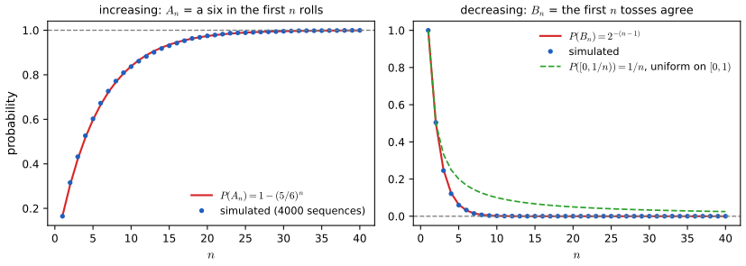
fig_1_s4. Supplementary figure (the book's Chapter 1 has no figures). Download: PDF · SVG1.4 Probability on Finite Sample Spaces
pp. 7–8 If \(\Omega=\{\omega_1,\dots,\omega_n\}\) is finite, a probability is determined by the \(n\) numbers \(p_i=\P(\{\omega_i\})\), which are nonnegative and sum to 1: by finite additivity \(\P(A)=\sum_{\omega_i\in A}p_i\). When all outcomes are equally likely, \(p_i=1/n\) and
\[ \P(A)=\frac{|A|}{|\Omega|}, \]the uniform distribution, and computing probabilities becomes counting. Rolling a die twice gives the 36 equally likely pairs \((i,j)\); the sum is 11 for \((5,6)\) and \((6,5)\), so its probability is \(2/36\). "Equally likely" is a modelling assumption about the outcomes, not about events: the eleven possible sums of two dice are not equally likely, and calling them the outcomes would give the wrong answer \(1/11\). The book recalls the number of orderings \(n!=n(n-1)\cdots2\cdot1\) (with \(0!=1\)) and
\[ \binom nk=\frac{n!}{k!\,(n-k)!}, \tag{1.2} \]"\(n\) choose \(k\)", the number of ways of choosing \(k\) objects out of \(n\); for instance, a committee of 3 from a class of 20 can be chosen in \(\binom{20}3\)
Result 1.F (the counting rules)
- Multiplication rule. If a choice is made in \(k\) stages and stage \(j\) has \(n_j\) options whatever was chosen before, there are \(n_1n_2\cdots n_k\) possible choices.
- Ordered samples. From \(n\) objects there are \(n^k\) ordered samples of size \(k\) with replacement, and \(n(n-1)\cdots(n-k+1)=n!/(n-k)!\) without replacement; \(n!\) orderings of all \(n\).
- Unordered samples without replacement. There are \(\binom nk\) subsets of size \(k\); \(\binom nk\)
\({}=\binom{n-1}k+\binom{n-1}{k-1}\) (Pascal's rule), \((a+b)^n=\sum_k\binom nka^kb^{n-k}\) (the binomial theorem) and \(\sum_k\binom nk=2^n\). - Unordered samples with replacement. There are \(\binom{n+k-1}k\) multisets of size \(k\) from \(n\) types.
Filling the gap 1.6: proofs of the counting rules, and the birthday problem pp. 7–8
Proof
(1) By induction on \(k\): each of the \(n_1\cdots n_{k-1}\) choices of the first \(k-1\) stages extends in exactly \(n_k\) ways. (2) With replacement, each of the \(k\) positions has \(n\) options; without replacement, position \(j\) has \(n-j+1\) options whatever was chosen before; taking \(k=n\) gives \(n!\). (3) Each subset of size \(k\) can be listed in \(k!\) orders, and each ordered sample without replacement arises from exactly one subset, so (number of subsets) \(\times k!=n!/(n-k)!\), which is (1.2). Pascal's rule: a \(k\)-subset of \(\{1,\dots,n\}\) either omits \(n\) (\(\binom{n-1}k\) of them) or contains it (\(\binom{n-1}{k-1}\) choices for the rest). Binomial theorem: expanding \((a+b)^n\) as a product of \(n\) factors, the term \(a^kb^{n-k}\) arises once for each choice of the \(k\) factors that contribute \(a\). With \(a=b=1\): \(\sum_k\binom nk=2^n\), the number of all subsets, each element being in or out. (4) A multiset of size \(k\) from \(n\) types is a row of \(k\) stars cut by \(n-1\) bars into \(n\) groups; it is fixed by the positions of the bars among \(n+k-1\) places. ∎
The birthday problem. With \(k\) people and 365 equally likely birthdays, the \(365^k\) ordered lists of birthdays are equally likely, and \(365\cdot364\cdots(365-k+1)\) of them have no repetition (rule 2). So \(\P(\text{a shared birthday})\)
1.5 Independent Events
Definition 1.9 (independence) p. 8, (1.3)
Two events \(A\) and \(B\) are independent, written \(A\indep B\), if
\[ \P(AB)=\P(A)\P(B). \tag{1.3} \]A family \(\{A_i:i\in I\}\) is independent if \(\P\big(\bigcap_{i\in J}A_i\big)\)
pp. 8–9 Independence enters in two ways. It is often assumed, as part of the model: a coin has no memory, so tosses are taken to be independent, and this assumption is what makes the probability of two heads \(\tfrac12\cdot\tfrac12\). It can also be found by checking (1.3): on a fair die, \(A=\{2,4,6\}\) and \(B=\{1,2,3,4\}\) have \(AB=\{2,4\}\) and \(\P(AB)=\tfrac13=\tfrac12\cdot\tfrac23\), so they are independent although nobody assumed it. Disjoint events with positive probabilities are never independent, since \(\P(AB)=\P(\varnothing)=0\lt\P(A)\P(B)\); apart from this case, a Venn diagram cannot show independence, which is a statement about sizes, not about shapes.
p. 9 In Example 1.10, ten tosses of a fair coin, "at least one head" is the complement of "all tails", and independence gives \(\P(\text{at least one head})\)
Filling the gap 1.7: the basketball game, completed p. 9, Example 1.11
Three points the example uses tacitly: the geometric series formula, the fact that the game ends, and a second derivation that avoids series altogether.
Derivation
The series. For \(0\lt r\lt1\), the partial sums satisfy \((1-r)\sum_{j=k}^{m}r^j=r^k-r^{m+1}\) (all middle terms cancel), and \(r^{m+1}\to0\), so \(\sum_{j=k}^\infty r^j=r^k/(1-r)\). With \(k=0\), \(r=\tfrac12\): \(\sum_j(\tfrac12)^{j-1}=2\) and the answer is \(\tfrac13\cdot2=\tfrac23\).
Why \(\P(A_j)\) is a product. \(A_j\) says that the first \(j-1\) rounds are double misses and person 1 then succeeds: \(2j-1\) attempts with prescribed results. The model takes the attempts to be independent (Definition 1.9 for the family of all attempts), so the probability of the intersection is the product \((2/3)^{j-1}(3/4)^{j-1}(1/3)\).
The game ends. Let \(N_m\) be the event that the first \(m\) rounds are all double misses; \(N_m\) decreases to the event that the game never ends, and \(\P(N_m)=(1/2)^m\to0\), so by continuity (Theorem 1.8) that event has probability 0. Person 2 wins first with probability \(\sum_j(\tfrac12)^{j-1}\tfrac23\cdot\tfrac14\)
First-step analysis. Let \(x\) be the answer. Either person 1 succeeds at once (probability \(\tfrac13\)), or round 1 is a double miss (probability \(\tfrac12\)) and, the later attempts being independent of round 1 and identically distributed, the game starts afresh, so person 1 then wins with probability \(x\); or person 2 wins in round 1. Hence \(x=\tfrac13+\tfrac12x\), i.e. \(x=\tfrac23\). In general, with success probabilities \(p_1,p_2\), \(x=p_1/\{1-(1-p_1)(1-p_2)\}\). A simulation of \(2\times10^5\) games gave \(0.666\). ∎
p. 10 To summarise: \(A\) and \(B\) are independent if and only if \(\P(AB)=\P(A)\P(B)\); independence is sometimes assumed and sometimes derived; and disjoint events with positive probability are dependent. For three or more events Definition 1.9 asks for many product rules, and they do not follow from one another.
Result 1.G (what independence of several events requires)
- Complements. If \(A_1,\dots,A_n\) are independent, so is any family obtained by replacing some of the \(A_i\) by their complements (Exercise 1.11 is the case \(n=2\)).
- Pairwise does not imply mutual. Toss a fair coin twice; let \(A\) = heads on toss 1, \(B\) = heads on toss 2, \(C\) = the two tosses agree. Each pair is independent, but \(\P(ABC)\)
\({}=\tfrac14\) \({}\ne\tfrac18\) \({}=\P(A)\P(B)\P(C)\). - The triple product does not imply pairwise. On \(\Omega=\{1,\dots,8\}\), uniform, \(A=\{1,2,3,4\}\), \(B=\{1,2,5,6\}\), \(C=\{1,3,7,8\}\) have \(\P(ABC)=\tfrac18=\P(A)\P(B)\P(C)\), but \(\P(BC)=\tfrac18\ne\tfrac14=\P(B)\P(C)\).
- Trivial events. An event with \(\P(A)\in\{0,1\}\) is independent of every event, and an event independent of itself has \(\P(A)\in\{0,1\}\) (Exercise 1.14).
- Counting the conditions. For \(n\) events, Definition 1.9 consists of \(2^n-n-1\) equations, one for each subset \(J\) with \(|J|\ge2\), and in general none of them can be dropped.
Filling the gap 1.8: proofs of Result 1.G
Proof
(1) It suffices to replace one event, say \(A_1\), by \(A_1^c\), and repeat. Take a finite \(J\). If \(1\notin J\) nothing changes. If \(1\in J\), let \(D=\bigcap_{i\in J,i\ne1}A_i\) (\(D=\Omega\) if \(J=\{1\}\)). Since \(D=A_1D\cup A_1^cD\) disjointly, with products over \(i\in J\), \(i\ne1\),
\[ \P(A_1^cD)=\P(D)-\P(A_1D)=\prod_{i\ne1}\P(A_i)-\P(A_1)\prod_{i\ne1}\P(A_i)=\P(A_1^c)\prod_{i\ne1}\P(A_i). \](2) The four outcomes have probability \(\tfrac14\) each; \(A=\{HH,HT\}\), \(B=\{HH,TH\}\), \(C=\{HH,TT\}\) each have probability \(\tfrac12\), and \(AB=AC=BC=ABC=\{HH\}\) have probability \(\tfrac14\). So the three pairwise equations hold and the triple one fails. In words: \(C\) is independent of \(A\) alone and of \(B\) alone, but \(A\) and \(B\) together determine \(C\). (This example goes back to S. N. Bernstein.)
(3) \(ABC=\{1\}\), probability \(\tfrac18=(\tfrac12)^3\); \(AB=\{1,2\}\) and \(AC=\{1,3\}\) have probability \(\tfrac14\) as required, but \(BC=\{1\}\).
(4) If \(\P(A)=0\), then \(0\le\P(AB)\le\P(A)=0=\P(A)\P(B)\). If \(\P(A)=1\), then \(\P(A^c)=0\), so \(A^c\) is independent of \(B\), hence so is \(A\) by part (1). Conversely, \(A\indep A\) means \(\P(A)=\P(AA)=\P(A)^2\), whose solutions are 0 and 1.
(5) There are \(2^n\) subsets of \(\{1,\dots,n\}\), of which \(n+1\) have fewer than two elements. That no equation follows from the others is shown, for \(n=3\), by examples (2) and (3): the pairwise equations do not give the triple one and the triple one does not give the pairwise ones. ∎
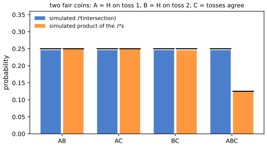
fig_1_s7. Supplementary figure. Download: PDF · SVGSee also (companion course): Foundations of Deep Learning, Section 2.1.6 (independence of random variables).
Independence and continuity together justify the frequency interpretation of Section 1.3. The next result is the first appearance of a theme of the whole book: a probability statement about one event ("the proportion after \(n\) tosses is far from \(p\)") is turned, through the axioms, into a statement about a whole infinite sequence.
Result 1.H (the Borel–Cantelli lemma and the strong law for coin tossing)
(a) If \(\sum_n\P(A_n)\lt\infty\), then \(\P(A_n\text{ infinitely often})\)
(b) Toss a coin with \(\P(\text{heads})=p\) independently forever, and let \(\hat p_n\) be the proportion of heads in the first \(n\) tosses. Then \(\P(\hat p_n\to p)=1\). More precisely, for every \(\eps\gt0\) and \(n\ge1\),
\[ \P\big(|\hat p_n-p|\gt\eps\big)\le\frac{p(1-p)}{n\eps^2}\quad\text{and}\quad\P\big(|\hat p_n-p|\gt\eps\big)\le\frac{7}{16\,n^2\eps^4}. \]Filling the gap 1.9: proof of Result 1.H with the tools of this chapter Exercises 1.3, 1.21
Only Theorem 1.8, Boole's inequality and independence are needed; the averages below are the expectations of Chapter 3, computed here as sums over a finite sample space.
Proof
(a) For every \(n\), \(\limsup_kA_k\subset\bigcup_{k\ge n}A_k\), so by Boole's inequality \(\P(\limsup A_k)\le\sum_{k\ge n}\P(A_k)\), the tail of a convergent series, which tends to 0.
(b), the setting. The event \(\{|\hat p_n-p|\gt\eps\}\) depends only on the first \(n\) tosses, whose outcomes \(x=(x_1,\dots,x_n)\in\{0,1\}^n\) (1 for heads) have probabilities \(\pi(x)=p^{s(x)}q^{n-s(x)}\), \(q=1-p\), \(s(x)=\sum_ix_i\), by independence. For a function \(g\) on \(\{0,1\}^n\) write \(\langle g\rangle=\sum_xg(x)\pi(x)\). If \(g\) depends only on \(x_i\) and \(h\) only on the other coordinates, then \(\pi\) factorises and \(\langle gh\rangle\)
A Markov-type bound. For \(k\ge1\), \(I\{|s-np|\)
Second moment.
\[ \Big\langle\Big(\sum_iy_i\Big)^2\Big\rangle=\sum_i\langle y_i^2\rangle+\sum_{i\ne j}\langle y_i\rangle\langle y_j\rangle=npq. \]With \(k=2\) this gives the first bound, Chebyshev's inequality for frequencies, and the weak law \(\P(|\hat p_n-p|\gt\eps)\to0\).
Fourth moment. Expanding \((\sum_iy_i)^4\), every term containing some \(y_i\) exactly once has average 0 by the product rule. What remains are the \(n\) terms \(y_i^4\) and, for each of the \(\binom n2\) pairs \(i\lt j\), the \(\binom42=6\) terms \(y_i^2y_j^2\):
\[ \Big\langle\Big(\sum_iy_i\Big)^4\Big\rangle=npq(1-3pq)+3n(n-1)p^2q^2=npq\{1+3(n-2)pq\}\le\frac n4+\frac{3n^2}{16}\le\frac{7n^2}{16}, \]using \(pq\le\tfrac14\). With \(k=4\): \(\P(|\hat p_n-p|\)
Almost sure convergence. Fix \(\eps\). The bounds \(7/(16n^2\eps^4)\) have a finite sum, so by (a) the event \(E_\eps\)
Remarks. The second-moment bound alone is not summable, which is why the fourth moment is used; Chapter 5 of the book proves the weak law in general, and the strong law for arbitrary independent averages needs more work. The existence of a probability on the infinite product space of Example 1.3 with the stated finite-dimensional probabilities is itself a theorem (Kolmogorov's extension theorem); here it is taken for granted, as in the book. The bound \(npq\{1+3(n-2)pq\}\) was confirmed against direct summation over the binomial distribution.
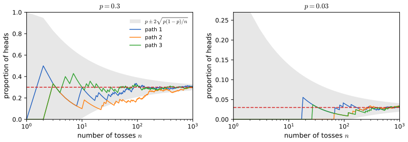
fig_1_s1. Supplementary figure. Download: PDF · SVGSee also (first-year notes): Section 0.3, Chebyshev's inequality and the weak law of large numbers for general averages.
1.6 Conditional Probability
Definition 1.12 (conditional probability) p. 10, (1.4)
If \(\P(B)\gt0\), the conditional probability of \(A\) given \(B\) is
\[ \P(A\given B)=\frac{\P(AB)}{\P(B)}. \tag{1.4} \]pp. 10–11 In frequency terms, \(\P(A\given B)\) is the proportion of the repetitions in which \(B\) occurs that also have \(A\). Conditioning restricts the sample space to \(B\) and rescales so that \(B\) has probability 1. Two warnings come with it. The rules of probability apply to the event on the left of the bar, not to the one on the right: in general \(\P(A\given B\cup C)\)
Result 1.J (conditional probability is a probability; the multiplication rule) Exercises 1.9, 1.17
(a) For fixed \(B\) with \(\P(B)\gt0\), \(A\mapsto\P(A\given B)\) satisfies Axioms 1 to 3, and therefore every result of Section 1.3 holds for it. For fixed \(A\), \(B\mapsto\P(A\given B)\) is in general not a probability.
(b) If \(\P(A_1\cdots A_{n-1})\gt0\), then
\[ \P(A_1A_2\cdots A_n)=\P(A_1)\P(A_2\given A_1)\P(A_3\given A_1A_2)\cdots\P(A_n\given A_1\cdots A_{n-1}). \]Filling the gap 1.10: proof of Result 1.J, and the counterexamples pp. 10–11
Proof
(a) Axiom 1: \(\P(AB)\ge0\) and \(\P(B)\gt0\). Axiom 2: \(\P(\Omega\given B)=\P(B)/\P(B)=1\). Axiom 3: if the \(A_i\) are disjoint, so are the \(A_iB\), and \(\big(\bigcup_iA_i\big)B\)
For the right-hand side: on a fair die let \(A=\{1\}\), \(B=\{1,2\}\), \(C=\{1,3\}\). Then \(\P(A\given B)=\P(A\given C)=\tfrac12\) but \(\P(A\given B\cup C)=\tfrac13\), not 1. Even for disjoint \(B\) and \(C\) additivity fails: \(\P(A\given\Omega)=\P(A)\), whereas additivity over the partition \(\{B,B^c\}\) would require \(\P(A\given B)+\P(A\given B^c)=\P(A)\); with \(A=B\) and \(0\lt\P(B)\lt1\) the left side is \(1\ne\P(B)\).
(b) By induction. For \(n=2\) it is (1.4) multiplied by \(\P(A_1)\). If it holds for \(n-1\), apply (1.4) to \(A_n\) and \(D=A_1\cdots A_{n-1}\): \(\P(DA_n)=\P(D)\P(A_n\given D)\). All the conditioning events \(A_1\cdots A_k\), \(k\le n-1\), contain \(D\) and so have positive probability. Exercise 1.17 is the case \(\P(ABC)\)
pp. 10–11 Example 1.13 is the lesson of the chapter. A test for a disease \(D\) has the joint probabilities
| \(D\) | \(D^c\) | total | |
|---|---|---|---|
| \(+\) | 0.009 | 0.099 | 0.108 |
| \(-\) | 0.001 | 0.891 | 0.892 |
| total | 0.010 | 0.990 | 1 |
so \(\P(+\given D)=0.009/0.010=0.9\) and \(\P(-\given D^c)=0.891/0.990=0.9\): the test is right 90% of the time for the sick and for the healthy. Yet
\[ \P(D\given+)=\frac{\P(+D)}{\P(+)}=\frac{0.009}{0.009+0.099}=\frac1{12}\approx0.083 . \]Among those testing positive, the healthy outnumber the sick 11 to 1, because healthy people are 99 times as common and 10% of them test positive.
Erratum (listed in the author's errata)
On p. 11 the second display reads \(\P(-\given D^c)\approx0.9\); the value is exactly \(0.891/0.990=0.9\), so "\(\approx\)" should be "\(=\)".
See also (companion course): Foundations of Deep Learning, Section 2.1.1 (the same lesson with a cancer screening test).
Lemma 1.14 p. 11
If \(A\) and \(B\) are independent and \(\P(B)\gt0\), then \(\P(A\given B)=\P(A)\). For any events with \(\P(A)\gt0\) and \(\P(B)\gt0\),
\[ \P(AB)=\P(A\given B)\P(B)=\P(B\given A)\P(A). \]Conversely, if \(\P(B)\gt0\) and \(\P(A\given B)=\P(A)\), then \(A\indep B\).
Proof (Exercise 1.16)
If \(A\indep B\), \(\P(A\given B)=\P(A)\P(B)/\P(B)=\P(A)\). The two product formulas are (1.4) for \(\P(A\given B)\) and for \(\P(B\given A)\), multiplied out (using \(AB=BA\)). Conversely, \(\P(A\given B)=\P(A)\) gives \(\P(AB)=\P(A\given B)\P(B)=\P(A)\P(B)\). ∎
A precision. The book states the lemma "for any pair of events", but \(\P(A\given B)\) is defined only when \(\P(B)\gt0\), and similarly for \(\P(B\given A)\); the same proviso applies to item 4 of its summary ("\(A\) and \(B\) are independent if and only if \(\P(A\given B)=\P(A)\)"). When \(\P(B)=0\), \(A\) and \(B\) are always independent (Result 1.G(4)) and the conditional probability is undefined. The product formula \(\P(AB)=\P(A)\P(B\given A)\) is the case \(n=2\) of Result 1.J(b).
p. 11 The product form is often the easiest route. In Example 1.15 two cards are drawn without replacement; the first is the ace of clubs with probability \(1/52\) and, given that, the second is the queen of diamonds with probability \(1/51\), so the probability of the pair is \(1/2652\). In short: \(\P(A\given B)=\P(AB)/\P(B)\) when \(\P(B)\gt0\); \(\P(\cdot\given B)\) is a probability for fixed \(B\) but \(\P(A\given\cdot)\) is not one for fixed \(A\); \(\P(A\given B)\) and \(\P(B\given A)\) differ in general; and, for \(\P(B)\gt0\), independence means \(\P(A\given B)=\P(A)\).
1.7 Bayes' Theorem
Theorem 1.16 (the law of total probability) p. 12
Let \(A_1,\dots,A_k\) be a partition of \(\Omega\) with \(\P(A_i)\gt0\) for each \(i\). Then for any event \(B\),
\[ \P(B)=\sum_{i=1}^k\P(B\given A_i)\P(A_i). \]The same holds for a countable partition \(A_1,A_2,\dots\) (a series of nonnegative terms).
Proof
The events \(C_i=BA_i\) are disjoint (they lie in disjoint \(A_i\)) and their union is \(B\cap\bigcup_iA_i=B\cap\Omega=B\) (distributive law). By additivity (finite, or Axiom 3 for a countable partition), \(\P(B)\)
A precision. The book does not require \(\P(A_i)\gt0\), but \(\P(B\given A_i)\) is undefined otherwise. Cells with \(\P(A_i)=0\) can simply be dropped, since \(\P(BA_i)\le\P(A_i)=0\); equivalently one may use the convention \(\P(B\given A_i)\P(A_i)=0\) for them.
Theorem 1.17 (Bayes' theorem) p. 12, (1.5)
Let \(A_1,\dots,A_k\) be a partition of \(\Omega\) with \(\P(A_i)\gt0\) for each \(i\). If \(\P(B)\gt0\), then for each \(i\),
\[ \P(A_i\given B)=\frac{\P(B\given A_i)\P(A_i)}{\sum_j\P(B\given A_j)\P(A_j)}. \tag{1.5} \]\(\P(A_i)\) is the prior probability of \(A_i\) and \(\P(A_i\given B)\) its posterior probability (Remark 1.18).
Proof
\(\P(A_i\given B)=\P(A_iB)/\P(B)\) by (1.4); the numerator is \(\P(B\given A_i)\P(A_i)\) by (1.4) again, and the denominator is the sum by Theorem 1.16. ∎
pp. 12–13 Example 1.19. E-mail falls into the classes \(A_1\) = spam, \(A_2\) = low priority, \(A_3\) = high priority with prior probabilities 0.7, 0.2 and 0.1, and \(B\) is the event that a message contains the word "free", with \(\P(B\given A_1)=0.9\), \(\P(B\given A_2)=0.01\), \(\P(B\given A_3)=0.01\). (The likelihoods need not sum to 1: they are probabilities of \(B\) under three different conditions.) Then
\[ \P(A_1\given B)=\frac{0.9\times0.7}{0.9\times0.7+0.01\times0.2+0.01\times0.1}=\frac{0.63}{0.633}=\frac{210}{211}\approx0.995 . \]Erratum (listed in the author's errata)
On p. 13 the three likelihoods are printed as \(\P(B\given A_1)=.9\), \(\P(B\given A_2)=.01\), \(\P(B\given A_1)=.01\); the second \(\P(B\given A_1)\) should be \(\P(B\given A_3)\), as the computation that follows uses.
Filling the gap 1.11: how the posterior depends on the base rate, and repeated evidence pp. 10–13
Example 1.13 says "don't trust your intuition" and computes one number. The formula behind it shows exactly when a positive test is convincing, and what a second test adds.
Derivation
Odds form. Dividing (1.5) for \(A_i\) by (1.5) for \(A_j\) cancels the denominator:
\[ \frac{\P(A_i\given B)}{\P(A_j\given B)}=\frac{\P(B\given A_i)}{\P(B\given A_j)}\cdot\frac{\P(A_i)}{\P(A_j)}: \]posterior odds = likelihood ratio \(\times\) prior odds. (The companion course derives this in full in Filling the gap 2.1 of Foundations of Deep Learning.)
The base-rate curve. For a test with sensitivity \(s=\P(+\given D)\), specificity \(c=\P(-\given D^c)\) and base rate \(\pi=\P(D)\),
\[ \P(D\given+)=\frac{\pi s}{\pi s+(1-\pi)(1-c)}=\frac{1}{1+\dfrac{1-\pi}{\pi}\cdot\dfrac{1-c}{s}} . \]The odds \((1-\pi)/\pi\) decrease in \(\pi\), so \(\P(D\given+)\) increases from 0 (as \(\pi\to0\)) to 1 (as \(\pi\to1\)); it exceeds \(\pi\) exactly when the likelihood ratio \(s/(1-c)\) exceeds 1, i.e. when the test is informative. A positive result makes the disease more likely than not exactly when \(\pi s\ge(1-\pi)(1-c)\), i.e.
\[ \pi\ge\pi^\ast=\frac{1-c}{s+1-c}. \]For the test of Example 1.13, \(s=c=0.9\) and \(\pi^\ast=0.1/1.0=0.1\): the condition must affect at least one person in ten before a positive result points more to disease than to health. At \(\pi=0.001\) the same test gives \(\P(D\given+)\approx0.009\).
Repeated tests. Suppose two tests are conditionally independent given the disease status: \(\P(+_1+_2\given D)\)
and conditional independence gives \(\P(+_2\given D+_1)=\P(+_2\given D)\). For Example 1.13 the odds go from \(1/99\) to \(9/99\) (posterior \(1/12\)) to \(81/99\) (posterior \(0.45\)) to \(729/99\) (posterior \(0.880\)). Conditional independence is an assumption about the tests: repeating the same test on the same sample would not satisfy it.
Evidence that lowers one class raises another (Exercise 1.18). If \(\P(A_1\given B)\lt\P(A_1)\), then \(\sum_{i\ge2}\P(A_i\given B)\)
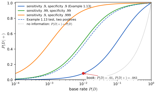
fig_1_s5. Supplementary figure. Download: PDF · SVGSee also (companion course): Foundations of Deep Learning, Section 2.1.4 (screening revisited) and Bayesian and Probabilistic Machine Learning, Definition 1.2 (Bayes' theorem as a rule for random variables).
The Monty Hall problem (Exercise 1.10) is Bayes' theorem in disguise: the prize is behind door \(i\) with prior probability \(\tfrac13\), the host's choice of door is the evidence, and its likelihood under each hypothesis depends on the host's rule. Under the standard rule the posterior probability of your own door stays at \(\tfrac13\), and switching wins with probability \(\tfrac23\); under other rules the answer changes, as the solution of Exercise 1.10 shows on the sample space of the book.
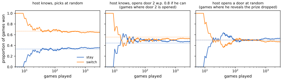
fig_1_s6, monty_exact. Supplementary figure. Download: PDF · SVG1.8 Bibliographic Remarks
p. 13 The material is standard. The book recommends DeGroot and Schervish (2002) at an introductory level, Grimmett and Stirzaker (1982) and Karr (1993) at an intermediate level, and Billingsley (1979) and Breiman (1992) at an advanced level, the last two for the measure theory sketched in the appendix. Many of the examples and exercises are adapted from DeGroot and Schervish and from Grimmett and Stirzaker.
1.9 Appendix
p. 13 On a finite or countable sample space every subset can be an event. On an uncountable one such as \([0,1)\) or \(\R\) this is impossible for the probabilities one wants (Result 1.L), and probabilities are assigned only to the events of a \(\sigma\)-field.
Definition 1.K (\(\sigma\)-field, measurable space, probability space) p. 13
A class \(\cA\) of subsets of \(\Omega\) is a \(\sigma\)-field (or \(\sigma\)-algebra) if (i) \(\varnothing\in\cA\); (ii) \(A_1,A_2,\dots\in\cA\) implies \(\bigcup_{i=1}^\infty A_i\in\cA\); (iii) \(A\in\cA\) implies \(A^c\in\cA\). Its members are the measurable sets (the events), \((\Omega,\cA)\) is a measurable space, and with a probability \(\P\) on \(\cA\) (Definition 1.5 for events in \(\cA\)) the triple \((\Omega,\cA,\P)\) is a probability space. The Borel \(\sigma\)-field \(\cB\) of \(\R\) is the smallest \(\sigma\)-field containing all open subsets of \(\R\).
Filling the gap 1.12: what a \(\sigma\)-field contains, "smallest", and the Borel sets p. 13
The book uses "the smallest \(\sigma\)-field that contains all the open subsets" without saying why it exists. Here are the closure properties, the existence of generated \(\sigma\)-fields, three descriptions of the Borel sets, and the countable case.
Proof
Closure. \(\Omega=\varnothing^c\in\cA\). Countable intersections: \(\bigcap_iA_i\)
Generated \(\sigma\)-fields. The intersection of any collection of \(\sigma\)-fields on \(\Omega\) is a \(\sigma\)-field (each of (i)–(iii) holds in every member, hence in the intersection). For a class \(\cG\) of subsets, the power set is a \(\sigma\)-field containing \(\cG\), so the intersection \(\sigma(\cG)\) of all \(\sigma\)-fields containing \(\cG\) is well defined; it contains \(\cG\) and is contained in every \(\sigma\)-field that contains \(\cG\): it is the smallest. \(\cB=\sigma(\text{open sets})\).
The Borel sets are generated by intervals. Let \(\cB'=\sigma(\{(a,b]:a\lt b\})\). Each \((a,b]=\bigcap_n(a,b+1/n)\) is a countable intersection of open sets, so \(\cB'\subset\cB\). Conversely, each open \(U\subset\R\) is the union of the open intervals with rational endpoints contained in it (around each point of \(U\) there is such an interval inside \(U\)), a countable union; and \((a,b)=\bigcup_n(a,b-1/n]\). So every open set is in \(\cB'\), and \(\cB\subset\cB'\). The same argument works with \((-\infty,x]\), \(x\in\R\): \((a,b]=(-\infty,b]-(-\infty,a]\). This is why a probability on \(\R\) can be described by the numbers \(F(x)=\P((-\infty,x])\), the cumulative distribution function of Chapter 2 (with uniqueness from Result 1.M).
Countable sample spaces. If \(\Omega\) is countable, every probability on the power set has the form \(\P(A)=\sum_{\omega\in A}p(\omega)\) with \(p(\omega)=\P(\{\omega\})\ge0\), \(\sum_\omega p(\omega)=1\) (countable additivity over the singletons of \(A\)); and every such \(p\) defines a probability on all subsets, since rearranging and grouping a series of nonnegative terms does not change its sum. So no \(\sigma\)-field restriction is needed there. ∎
Result 1.L (not every subset can have a probability: Vitali, 1905)
There is no function \(\P\), defined on all subsets of \([0,1)\), that satisfies Axioms 1 to 3 and is invariant under rotation: \(\P(A\oplus r)=\P(A)\) for every \(A\) and every \(r\in[0,1)\), where \(A\oplus r=\{(x+r)\bmod1:x\in A\}\).
The uniform distribution on \([0,1)\) (length, \(\P((a,b])=b-a\)) is rotation invariant on the Borel sets, so it cannot be extended to all subsets.
Proof
A Vitali set. Call \(x,y\in[0,1)\) equivalent if \(x-y\) is rational. This is an equivalence relation, and it splits \([0,1)\) into disjoint classes \(x+\Q\) (intersected with \([0,1)\)), uncountably many, each countable. Using the axiom of choice, let \(V\) contain exactly one point of each class.
Countably many disjoint rotated copies cover \([0,1)\). For each rational \(r\in\Q\cap[0,1)\), a countable set, let \(V_r=V\oplus r\). Disjoint: if \(x\in V_r\cap V_s\), then \(x\equiv v+r\equiv w+s\pmod1\) with \(v,w\in V\), so \(v-w\) is rational, \(v\) and \(w\) are equivalent and, since \(V\) has one point per class, \(v=w\); then \(r\equiv s\pmod1\), i.e. \(r=s\). Cover: for \(x\in[0,1)\) let \(v\in V\) be the representative of its class; \(x-v\in\Q\cap(-1,1)\), and with \(r=(x-v)\bmod1\in\Q\cap[0,1)\) we get \(x=v\oplus r\in V_r\).
Contradiction. If \(\P\) existed, Axioms 2 and 3 and invariance would give \(1=\P([0,1))=\sum_r\P(V_r)=\sum_r\P(V)\), a countable sum of equal terms, which is 0 or \(\infty\). ∎
Remarks. The rotation invariance of length on the Borel sets follows from Result 1.M: \(A\mapsto\P(A\oplus r)\) and \(\P\) agree on intervals (a rotated interval is an interval, or two intervals of the same total length). The obstacle is not invariance alone: under the continuum hypothesis, Banach and Kuratowski (1929) showed that no probability on all subsets of \([0,1]\) gives every single point probability 0. And the axiom of choice cannot be avoided: Solovay (1970) constructed models of set theory without full choice in which every subset of \(\R\) is Lebesgue measurable.
Result 1.M (a probability is determined by its values on intervals)
(a) Uniqueness. If two probabilities on \(\sigma(\cP)\) agree on a class \(\cP\) closed under finite intersections (a \(\pi\)-system), they agree on \(\sigma(\cP)\). In particular a probability on \((\R,\cB)\) is determined by its values on the intervals \((-\infty,x]\).
(b) Existence (Lebesgue; Carathéodory's extension theorem). There is a probability on the Borel sets of \([0,1)\) with \(\P((a,b])=b-a\) for all \(0\le a\lt b\le1\), the uniform distribution of Chapter 2.
Filling the gap 1.13: Dynkin's \(\pi\)–\(\lambda\) theorem, and an outline of Carathéodory's construction
The book's appendix stops at the definition of the Borel \(\sigma\)-field. These two facts are what make it usable: uniqueness is proved in full; existence is outlined.
Proof of (a), outline of (b)
\(\lambda\)-systems. A class \(\cL\) is a \(\lambda\)-system if \(\Omega\in\cL\); \(A,B\in\cL\) and \(A\subset B\) imply \(B-A\in\cL\); and \(A_n\in\cL\), \(A_n\uparrow A\) imply \(A\in\cL\). A class that is both a \(\pi\)-system and a \(\lambda\)-system is a \(\sigma\)-field: it contains \(\varnothing=\Omega-\Omega\) and complements \(A^c=\Omega-A\), hence finite unions \(A\cup B=(A^cB^c)^c\), and countable unions as increasing limits of finite unions.
Dynkin's theorem: if \(\cP\) is a \(\pi\)-system contained in a \(\lambda\)-system \(\cL\), then \(\sigma(\cP)\subset\cL\). Let \(\ell\) be the smallest \(\lambda\)-system containing \(\cP\) (the intersection of all of them, which is again a \(\lambda\)-system). It suffices to show that \(\ell\) is a \(\pi\)-system, for then it is a \(\sigma\)-field containing \(\cP\), so \(\sigma(\cP)\subset\ell\subset\cL\). For \(A\in\ell\) let \(\cG_A=\{B:AB\in\ell\}\). Then \(\cG_A\) is a \(\lambda\)-system: \(A\Omega=A\in\ell\); if \(B\subset C\) are in \(\cG_A\), then \(A(C-B)=AC-AB\) with \(AB\subset AC\) both in \(\ell\); if \(B_n\uparrow B\) in \(\cG_A\), then \(AB_n\uparrow AB\). If \(A\in\cP\), then \(\cP\subset\cG_A\) (\(\cP\) is a \(\pi\)-system), so \(\ell\subset\cG_A\): \(AB\in\ell\) for \(A\in\cP\), \(B\in\ell\). This says that for \(B\in\ell\), \(\cP\subset\cG_B\); hence \(\ell\subset\cG_B\), i.e. \(\ell\) is closed under intersections.
Proof of (a). Let \(\cL\)
Outline of (b). Define the outer measure \(\lambda^\ast(A)=\inf\sum_i(b_i-a_i)\) over all countable covers of \(A\subset[0,1)\) by intervals \((a_i,b_i]\). The sets \(E\) that split every set additively, \(\lambda^\ast(A)\)
1.10 Exercises
pp. 13–17 Each exercise is restated in my own words, followed by a complete solution. Computational answers were checked with the Python code using exact fractions.
Exercise 1.1. Complete the proof of Theorem 1.8, and prove the case of a decreasing sequence.
Solution
Both parts are in the proof under Theorem 1.8: the sets \(B_n=A_n-A_{n-1}\) are shown to be disjoint, to have \(\bigcup_{i\le n}B_i=A_n\) (by induction) and \(\bigcup_iB_i=\bigcup_iA_i\) (via the first index at which an outcome enters); the decreasing case follows by complements and De Morgan. Filling the gap 1.4 extends the theorem to all convergent sequences.
Exercise 1.2. Prove the statements in (1.1).
Solution
See Filling the gap 1.2. The key step is \(\P(\varnothing)=0\), obtained from Axiom 3 applied to infinitely many empty sets; finite additivity, monotonicity, \(0\le\P\le1\) and the complement rule follow.
Exercise 1.3. For events \(A_1,A_2,\dots\) let \(B_n=\bigcup_{i\ge n}A_i\) and \(C_n=\bigcap_{i\ge n}A_i\). (a) Show that the \(B_n\) decrease and the \(C_n\) increase. (b) Show that \(\omega\in\bigcap_nB_n\) iff \(\omega\) belongs to infinitely many \(A_i\). (c) Show that \(\omega\in\bigcup_nC_n\) iff \(\omega\) belongs to all but finitely many \(A_i\).
Solution
(a) \(B_n=A_n\cup B_{n+1}\supset B_{n+1}\) and \(C_n=A_n\cap C_{n+1}\subset C_{n+1}\). (b) \(\omega\in\bigcap_nB_n\) iff for every \(n\) some \(i\ge n\) has \(\omega\in A_i\), iff \(\{i:\omega\in A_i\}\) has no largest element, iff it is infinite. (c) \(\omega\in\bigcup_nC_n\) iff for some \(n\), \(\omega\in A_i\) for every \(i\ge n\), iff the indices with \(\omega\notin A_i\) are all below some \(n\), iff there are finitely many of them. So \(\bigcap_nB_n=\limsup A_n\) and \(\bigcup_nC_n=\liminf A_n\) (Definition 1.A, Filling the gap 1.1).
Exercise 1.4. For any index set \(I\), show that \(\big(\bigcup_{i\in I}A_i\big)^c\)
\({}=\bigcap_{i\in I}A_i^c\) and \(\big(\bigcap_{i\in I}A_i\big)^c\) \({}=\bigcup_{i\in I}A_i^c\). Solution
See Filling the gap 1.1: \(\omega\) is outside the union iff it is outside every \(A_i\); the second law is the first applied to the complements. The pointwise argument covers finite, countable and uncountable \(I\) at once, so the hint (first prove it for \(I=\{1,\dots,n\}\)) is not needed.
Exercise 1.5. A fair coin is tossed until exactly two heads have appeared. Describe the sample space and find the probability that exactly \(k\) tosses are needed.
Solution
\(\Omega\) is the set of finite \(H/T\) strings that contain exactly two heads and end with a head, e.g. \(HH\), \(THH\), \(HTH\), \(TTHTH\), ... (and, if one wants a complete description, the infinite strings with at most one head, which have probability 0 by continuity). A string of length \(k\ge2\) qualifies iff its last toss is a head and exactly one of the first \(k-1\) is a head: \(k-1\) strings, each of probability \(2^{-k}\). So \(\P(\text{exactly }k\text{ tosses})\)
\({}=(k-1)/2^k\), \(k=2,3,\dots\). Check: \(\sum_{k\ge2}(k-1)2^{-k}\) \({}=\sum_{m\ge1}m2^{-m-1}\) \({}=\tfrac12\cdot2\) \({}=1\), using \(\sum_mmx^m=x/(1-x)^2\) at \(x=\tfrac12\). Exercise 1.6. Let \(\Omega=\{0,1,2,\dots\}\). Prove that there is no uniform distribution on \(\Omega\): if \(\P(A)=\P(B)\) whenever \(|A|=|B|\), then \(\P\) cannot satisfy the axioms.
Solution
All singletons have the same size, hence the same probability \(c\ge0\). By Axiom 3 over the disjoint singletons, \(1=\P(\Omega)=\sum_{k=0}^\infty c\), which is 0 if \(c=0\) and infinite if \(c\gt0\). See Filling the gap 1.5 for why a merely finitely additive "uniform distribution" exists but is not continuous.
Exercise 1.7. Show that \(\P\big(\bigcup_{n=1}^\infty A_n\big)\)
\({}\le\sum_{n=1}^\infty\P(A_n)\) for any events. Solution
This is Boole's inequality, Result 1.D, proved with the hint's sets \(B_n=A_n-\bigcup_{i\lt n}A_i\), which are disjoint, satisfy \(B_n\subset A_n\) and have the same union as the \(A_n\).
Exercise 1.8. If \(\P(A_i)=1\) for every \(i\), prove that \(\P\big(\bigcap_{i=1}^\infty A_i\big)=1\).
Solution
By De Morgan and Boole, \(\P\big((\bigcap_iA_i)^c\big)\)
\({}=\P\big(\bigcup_iA_i^c\big)\) \({}\le\sum_i\P(A_i^c)\) \({}=\sum_i0\) \({}=0\). So the complement has probability 0 and the intersection probability 1 (Result 1.D). Exercise 1.9. For fixed \(B\) with \(\P(B)\gt0\), show that \(\P(\cdot\given B)\) satisfies the axioms of probability.
Solution
See Result 1.J(a) and Filling the gap 1.10: nonnegativity is clear, \(\P(\Omega\given B)=1\), and for disjoint \(A_i\) the sets \(A_iB\) are disjoint with union \((\bigcup A_i)B\), so countable additivity carries over after dividing by \(\P(B)\).
Exercise 1.10 (the Monty Hall problem, posed in this form by Selvin, 1975). A prize is placed behind one of three doors at random; you pick door 1; the host, who knows where the prize is, opens one of the other two doors and shows that it is empty, then offers you the remaining closed door. Show that you should switch, working on the sample space \(\Omega=\{(\omega_1,\omega_2)\}\) where \(\omega_1\) is the prize door and \(\omega_2\) the door the host opens.
Solution
The model. \(\P(\omega_1=i)=\tfrac13\) for \(i=1,2,3\). The host never opens door 1 or the prize door. If \(\omega_1=2\) he must open 3; if \(\omega_1=3\) he must open 2; if \(\omega_1=1\) he opens 2 or 3, and the standard assumption is that he chooses at random. The outcomes with positive probability are
\[ \P(1,2)=\P(1,3)=\tfrac13\cdot\tfrac12=\tfrac16,\qquad\P(2,3)=\tfrac13,\qquad\P(3,2)=\tfrac13 . \]Conditioning. Suppose the host opens door 3, the event \(\{\omega_2=3\}=\{(1,3),(2,3)\}\), of probability \(\tfrac16+\tfrac13=\tfrac12\). Then
\[ \P(\omega_1=1\given\omega_2=3)=\frac{1/6}{1/2}=\frac13,\qquad \P(\omega_1=2\given\omega_2=3)=\frac{1/3}{1/2}=\frac23, \]and by symmetry the same when he opens door 2. Switching wins with probability \(\tfrac23\) whatever door he opens. The intuition "two doors left, so \(\tfrac12\)" treats the host's choice as uninformative; but he is forced to avoid the prize, so the door he leaves closed carries the \(\tfrac23\) of the two doors you did not pick.
The rule matters. If, with the prize behind door 1, the host opens door 2 with probability \(q\) (instead of \(\tfrac12\)), then \(\P(1,2)=q/3\), \(\P(1,3)=(1-q)/3\), and
\[ \P(\text{switch wins}\given\omega_2=2)=\frac{1/3}{1/3+q/3}=\frac1{1+q},\qquad \P(\text{switch wins}\given\omega_2=3)=\frac1{2-q}, \]both at least \(\tfrac12\): switching is never worse, and is a sure win if \(q=1\) and he opens door 3. If the host does not know where the prize is and opens door 2 or 3 at random, then given that the opened door is empty the six equally likely pairs reduce to \((1,2),(1,3),(2,3),(3,2)\), each with probability \(\tfrac16\), and staying and switching both win with probability \(\tfrac12\). With \(d\) doors and a knowing host who opens \(d-2\) of them, switching wins with probability \((d-1)/d\). These values were obtained by enumerating the sample space with exact fractions (
monty_exact) and are illustrated in Figure 1.S6.Exercise 1.11. If \(A\) and \(B\) are independent, show that \(A^c\) and \(B^c\) are independent.
Solution
\(\P(A^cB^c)\)
\({}=\P\big((A\cup B)^c\big)\) \({}=1-\P(A)-\P(B)+\P(AB)\) \({}=1-\P(A)-\P(B)+\P(A)\P(B)\) \({}=(1-\P(A))(1-\P(B))\) \({}=\P(A^c)\P(B^c)\), using De Morgan, Lemma 1.6 and independence. The general statement is Result 1.G(1). Exercise 1.12. Three cards: one green on both sides, one red on both sides, one green on one side and red on the other. A card is chosen at random and one of its sides, also at random, is shown. If the side shown is green, what is the probability that the other side is green?
Solution
The six (card, side) pairs are equally likely. Three of them show green: both sides of the green card and the green side of the mixed card. In two of these three the other side is green. So the answer is \(\tfrac23\). With Bayes' theorem,
\[ \P(GG\given\text{green})=\frac{1\cdot\frac13}{1\cdot\frac13+0\cdot\frac13+\frac12\cdot\frac13}=\frac23. \]The answer \(\tfrac12\) comes from conditioning on "the card is not red-red" instead of on what was seen: the green card is twice as likely as the mixed card to show green.
Exercise 1.13. A fair coin is tossed until both a head and a tail have appeared. (a) Describe the sample space. (b) Find the probability that exactly three tosses are needed.
Solution
(a) \(\Omega\)
\({}=\{H^kT:k\) \({}\ge1\}\cup\{T^kH:k\) \({}\ge1\}\), where \(H^kT\) is \(k\) heads followed by a tail (plus the two infinite constant sequences, of probability 0). (b) Three tosses are needed exactly for \(HHT\) and \(TTH\), so the probability is \(\tfrac18+\tfrac18=\tfrac14\). In general \(\P(k\text{ tosses})\) \({}=2\cdot2^{-k}\) \({}=2^{1-k}\) for \(k\ge2\), and these sum to 1. Exercise 1.14. Show that an event with \(\P(A)=0\) or \(\P(A)=1\) is independent of every event, and that an event independent of itself has probability 0 or 1.
Solution
See Result 1.G(4) and its proof in Filling the gap 1.8.
Exercise 1.15. Each child independently has blue eyes with probability \(\tfrac14\). In a family of three children, find the probability that at least two have blue eyes, (a) given that at least one has blue eyes, (b) given that the youngest has blue eyes.
Solution
Let \(N\) be the number of blue-eyed children; \(\P(N\)
\({}=k)\) \({}=\binom3k(\tfrac14)^k(\tfrac34)^{3-k}\), i.e. \(\tfrac{27}{64}\), \(\tfrac{27}{64}\), \(\tfrac{9}{64}\), \(\tfrac1{64}\) for \(k=0,1,2,3\). (a) \(\P(N\) \({}\ge2\given N\) \({}\ge1)\) \({}=\frac{10/64}{37/64}\) \({}=\frac{10}{37}\) \({}\approx0.270\). (b) Given that the youngest is blue-eyed, at least two are iff at least one of the other two is, and by independence that has probability \(1-(\tfrac34)^2=\tfrac7{16}\approx0.438\). Knowing which child is blue-eyed is more informative than knowing that some child is. Exercise 1.16. Prove Lemma 1.14.
Solution
See the proof under Lemma 1.14, which also records the positivity conditions the statement needs.
Exercise 1.17. Show that \(\P(ABC)\)
\({}=\P(A\given BC)\P(B\given C)\P(C)\). Solution
For \(\P(BC)\gt0\): \(\P(A\given BC)\P(BC)=\P(ABC)\) and \(\P(BC)=\P(B\given C)\P(C)\) by (1.4) twice. (If \(\P(BC)=0\) the left side is 0 and the right side contains an undefined factor.) This is Result 1.J(b) with \(n=3\).
Exercise 1.18. Let \(A_1,\dots,A_k\) be a partition of \(\Omega\) and \(\P(B)\gt0\). Prove that if \(\P(A_1\given B)\lt\P(A_1)\), then \(\P(A_i\given B)\gt\P(A_i)\) for some \(i\in\{2,\dots,k\}\).
Solution
Both \(\P\) and \(\P(\cdot\given B)\) are probabilities, so \(\sum_{i=1}^k\P(A_i)\)
\({}=\sum_{i=1}^k\P(A_i\given B)\) \({}=1\). Subtracting, \(\sum_{i\ge2}\{\P(A_i\given B)-\P(A_i)\}\) \({}=\P(A_1)-\P(A_1\given B)\) \({}\gt0\), so at least one term of the left sum is positive (see also Filling the gap 1.11). Exercise 1.19. 30% of computer owners use a Macintosh, 50% Windows and 20% Linux; 65%, 82% and 50% of them respectively have caught a virus. A randomly chosen person's computer is infected. What is the probability that she uses Windows?
Solution
By the law of total probability \(\P(V)\)
\({}=0.3\cdot0.65+0.5\cdot0.82+0.2\cdot0.5\) \({}=0.195+0.41+0.1\) \({}=0.705\), and by Bayes' theorem \(\P(W\given V)\) \({}=0.41/0.705\) \({}=82/141\) \({}\approx0.582\). (Similarly \(\P(\text{Mac}\given V)\approx0.277\) and \(\P(\text{Linux}\given V)\approx0.142\).) Exercise 1.20. A box holds five coins with probabilities of heads \(p_1=0\), \(p_2=\tfrac14\), \(p_3=\tfrac12\), \(p_4=\tfrac34\), \(p_5=1\). Let \(C_i\) be the event that coin \(i\) is chosen and \(H_j\) that toss \(j\) gives heads. (a) A coin is chosen at random and tossed once, giving heads; find \(\P(C_i\given H_1)\). (b) Find \(\P(H_2\given H_1)\). (c) If instead the chosen coin is tossed until the first head, and \(B_4\) is the event that this happens on toss 4, find \(\P(C_i\given B_4)\).
Solution
Tosses of the chosen coin are independent given the coin. (a) \(\P(H_1)\)
\({}=\sum_i\tfrac15p_i\) \({}=\tfrac15\cdot\tfrac52\) \({}=\tfrac12\), so \(\P(C_i\given H_1)\) \({}=\frac{p_i/5}{1/2}\) \({}=\frac{2p_i}5\): \(0,\ 0.1,\ 0.2,\ 0.3,\ 0.4\). (b) \(\P(H_1H_2)\) \({}=\sum_i\tfrac15p_i^2\) \({}=\tfrac15(0+\tfrac1{16}\) \({}+\tfrac14+\tfrac9{16}+1)\) \({}=\tfrac38\), so \(\P(H_2\given H_1)\) \({}=\frac{3/8}{1/2}\) \({}=\frac34\); equivalently \(\sum_ip_i\P(C_i\given H_1)=\tfrac34\), the average of \(p_i\) under the posterior. The first head raises the chance of the second from \(\tfrac12\) to \(\tfrac34\): given the coin the tosses are independent, but without knowing the coin they are not. (c) \(\P(B_4\given C_i)=(1-p_i)^3p_i\): \(0\), \(\tfrac{27}{256}\), \(\tfrac{16}{256}\), \(\tfrac3{256}\), \(0\). The priors are equal, so the posteriors are these numbers normalised: \(\P(C_i\given B_4)\) is \(0\), \(\tfrac{27}{46}\), \(\tfrac8{23}\), \(\tfrac3{46}\), \(0\) \({}\approx0,\ 0.587,\ 0.348,\ 0.065,\ 0\). 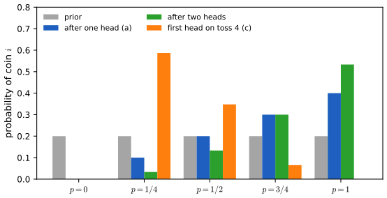
Figure 1.S8. Exercise 1.20: the posterior probability of each coin after one head (part (a)), after two heads, and after a first head on toss 4 (part (c)). Heads push the posterior toward the high-\(p\) coins; three tails before a head push it toward \(p=\tfrac14\), and rule out the two deterministic coins. Code: fig_1_s8,ex_1_20. Supplementary figure. Download: PDF · SVG▶ DemoExercise 1.20(c): first head on toss 4Switch the evidence to one or two heads to reproduce parts (a) and (b).Exercise 1.21 (computer experiment). Simulate \(n=1000\) tosses of a coin with \(p=0.3\) and plot the proportion of heads against \(n\). Repeat with \(p=0.03\).
Solution
Figure 1.S1 shows three runs for each \(p\) (function
ex_1_21). After 1000 tosses the proportions were 0.304, 0.299, 0.298 for \(p=0.3\) and 0.030, 0.033, 0.032 for \(p=0.03\), within the band \(p\pm2\sqrt{p(1-p)/n}\) (\(\pm0.029\) and \(\pm0.011\)). For \(p=0.03\) the path sits at 0 until the first head (on average after 33 tosses) and the relative error \(\sqrt{(1-p)/(np)}\approx0.18\) at \(n=1000\) is much larger than for \(p=0.3\) (\(0.048\)): rare events need many more trials to estimate to the same relative accuracy. The convergence itself is Result 1.H.Exercise 1.22 (computer experiment). Let \(X\) be the number of heads in \(n\) tosses with \(\P(\text{heads})=p\). Repeat the experiment many times and compare the average of the \(X\)'s with \(np\), for \(p=0.3\) and \(n=10,100,1000\).
Solution
With 2000 repetitions (function
ex_1_22) the averages were \(2.99\), \(30.01\) and \(299.54\), against \(np=3\), 30 and 300. The individual \(X\)'s spread around \(np\) with standard deviation close to \(\sqrt{np(1-p)}\) (1.46, 4.72, 14.21 simulated against 1.45, 4.58, 14.49), so the average of 2000 of them has standard deviation about \(\sqrt{np(1-p)/2000}\) (0.03, 0.10, 0.32), and each average is within about 1.5 of these of \(np\). Figure 1.S2 shows the three histograms. The intuition "\(X\) is close to \(np\)" is right for the average and for the proportion \(X/n\), but \(X\) itself deviates from \(np\) by more as \(n\) grows (like \(\sqrt n\)).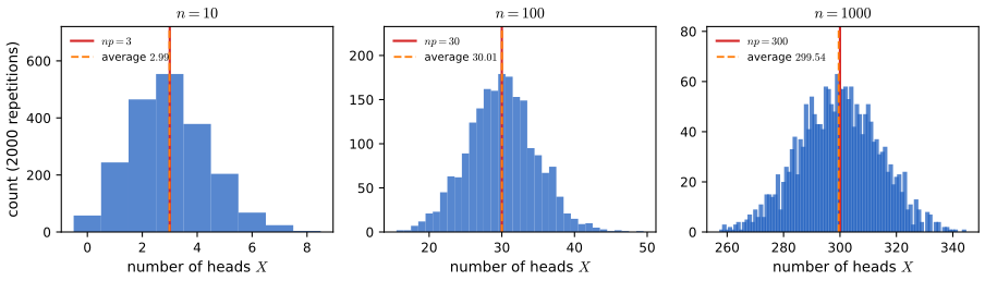
Figure 1.S2. Exercise 1.22: 2000 simulated values of the number of heads \(X\) in \(n\) tosses with \(p=0.3\); red, \(np\); dashed, the average of the 2000 values. Code: fig_1_s2. Supplementary figure. Download: PDF · SVGExercise 1.23 (computer experiment). On a fair die, \(A=\{2,4,6\}\) and \(B=\{1,2,3,4\}\) are independent: \(\P(A)=\tfrac12\), \(\P(B)=\tfrac23\), \(\P(AB)=\tfrac13\). Simulate rolls and compare the relative frequencies of \(A\), \(B\) and \(AB\) with these values and with \(\hat\P(A)\hat\P(B)\). Then find two dependent events and do the same.
Solution
With 20,000 simulated rolls (function
ex_1_23): \(\hat\P(A)=0.4998\), \(\hat\P(B)=0.6732\), \(\hat\P(AB)=0.3368\) and \(\hat\P(A)\hat\P(B)=0.3364\), so the two sides of (1.3) agree to within \(4\times10^{-4}\), less than the sampling error of either (about \(0.003\)). For the dependent pair \(A=\{2,4,6\}\), \(B=\{1,2,3\}\), with \(\P(AB)=\tfrac16\) and \(\P(A)\P(B)=\tfrac14\): \(\hat\P(AB)=0.1673\) and \(\hat\P(A)\hat\P(B)=0.2517\), a difference far beyond sampling error. Interpretation: simulation estimates each probability with error of order \(1/\sqrt n\), so it can reveal a dependence of size much larger than \(1/\sqrt n\) but can never prove exact independence, which is an equation between numbers. Figure 1.S3 follows both comparisons as the number of rolls grows.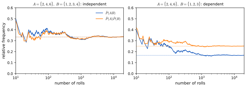
Figure 1.S3. Exercise 1.23: running relative frequency of \(AB\) (blue) and product of the relative frequencies of \(A\) and \(B\) (orange) for an independent pair (left) and a dependent pair (right) of events on a die; dotted lines are the exact values. Code: fig_1_s3. Supplementary figure. Download: PDF · SVG▶ DemoA dependent pair on a dieThe frequency difference leaves the chance band and settles at −1/12.
Demonstrations for this chapter
| Demonstration | What you can see | Sections and results |
|---|---|---|
| Bayes' theorem over a partition: base rates | The probability square (column widths = priors, shaded heights = likelihoods), prior against posterior, the posterior against the base rate, and simulated long-run frequencies. Presets: 1 Example 1.13; 2 two positive tests; 3 Example 1.19; 4 Exercise 1.19; 5 Exercise 1.20(c). | 1.6, 1.7; Theorem 1.17, Filling the gap 1.11 |
| Independence: pairwise against mutual | Build events on a die, two or three coins or eight outcomes; exact product tests for every pair and the triple; simulated frequency differences against a chance band. Presets: 1 Exercise 1.23; 2 a dependent pair; 3 Bernstein's example; 4 triple product only; 5 three coins. | 1.5; Definition 1.9, Result 1.G |
| Long-run frequencies and continuity | Running proportions of heads for up to 400 coins; the probability of being more than \(\eps\) from \(p\) at toss \(n\) (exact binomial, Chebyshev, simulated); the nested events "outside at some later toss". Presets: 1 and 2 Exercise 1.21; 3 the weak law; 4 continuity; 5 a narrow band. | 1.3; Theorem 1.8, Result 1.H |
| The Monty Hall problem | The sample space table with the observed event outlined, the doors of the last game, and win proportions of staying and switching. Presets: 1 Exercise 1.10; 2 ten doors; 3 and 4 a host who prefers door 2; 5 an ignorant host. | 1.7; Exercise 1.10 |
The Python code that produces every figure of this page and the simulations behind the demonstrations is code/ch01_probability.py (see the code index). A demonstration of Bayes' theorem with counts in a population, and of updating for a bent coin, is in the companion course: medical screening and the bent coin.
References
- Wasserman, L. (2004). All of Statistics: A Concise Course in Statistical Inference. Springer, New York. Chapter 1, pp. 3–17. www.stat.cmu.edu/~larry/all-of-statistics.
- Banach, S. and Kuratowski, C. (1929). Sur une généralisation du problème de la mesure. Fundamenta Mathematicae, 14, 127–131.
- Billingsley, P. (1995). Probability and Measure, 3rd edition. Wiley, New York. (First edition 1979.)
- Breiman, L. (1992). Probability. SIAM, Philadelphia. (Reprint of the 1968 edition.)
- DeGroot, M. H. and Schervish, M. J. (2002). Probability and Statistics, 3rd edition. Addison-Wesley, Boston.
- Dynkin, E. B. (1965). Markov Processes, Volume 1. Springer, Berlin.
- Grimmett, G. R. and Stirzaker, D. R. (1982). Probability and Random Processes. Oxford University Press.
- Karr, A. F. (1993). Probability. Springer, New York.
- Kolmogorov, A. N. (1933). Grundbegriffe der Wahrscheinlichkeitsrechnung. Springer, Berlin.
- Selvin, S. (1975). A problem in probability (letter). The American Statistician, 29(1), 67.
- Solovay, R. M. (1970). A model of set-theory in which every set of reals is Lebesgue measurable. Annals of Mathematics, 92(1), 1–56.
- Vitali, G. (1905). Sul problema della misura dei gruppi di punti di una retta. Tipografia Gamberini e Parmeggiani, Bologna.
The numerical statements in the text (the exact answers to the examples and exercises, inclusion–exclusion and the matching probabilities, the independence tables, the binomial moment bounds, the Monty Hall probabilities and the simulated frequencies) were confirmed numerically.