Models, Statistical Inference and Learning
This short chapter is the hinge of the book: it leaves probability behind and sets up the vocabulary of inference. A statistical model is a set of candidate distributions, finite-dimensional (parametric) or not (nonparametric). Inference then comes in three forms: a single best guess (point estimation), a set that traps the unknown with a guaranteed frequency (confidence sets), and a yes-or-no verdict on a default theory (hypothesis testing). The book states the key facts in a few lines each; these notes prove them, show where they break (an estimator that never settles, an interval whose coverage collapses near the edge of the parameter space, a Bayesian interval with poor frequentist coverage), and quantify everything with exact calculations.
Ch. 1 Probability Ch. 2 Random variables Ch. 3 Expectation Ch. 4 Inequalities Ch. 5 Convergence Ch. 6 Models and inference Ch. 7 Estimating the CDF Ch. 8 Bootstrap Ch. 9 Parametric inference Ch. 10 Hypothesis testing Ch. 11 Bayesian inference Ch. 12 Decision theory Ch. 13 Regression Ch. 14 Multivariate models Ch. 15 Independence Ch. 16 Causal inference Ch. 17 Directed graphs Ch. 18 Undirected graphs Ch. 19 Log-linear models Ch. 20 Curve estimation Ch. 21 Orthogonal functions Ch. 22 Classification Ch. 23 Stochastic processes Ch. 24 Simulation
How to read these notes
They follow the book. Sections carry the book's numbers (6.2, 6.3.1, ...) and every displayed equation that appears in the book carries the book's own equation number, e.g. \((6.7)\). Numbered items keep the book's numbers (Definition 6.7, Theorem 6.9, Example 6.14); definitions the book states without a number are lettered (Definition 6.A, 6.B, ...). Equations without a number are steps that the book skips.
Filling the gaps. Wherever the book says "you can check", quotes a fact without proof, or leaves an argument implicit, an orange Filling the gap box gives the full argument. Proofs and derivations start hidden: open one with its bar, or use the button below.
Figures and demonstrations. Chapter 6 of the book has no figures. The six figures here are supplementary (numbered 6.S1 to 6.S6): each illustrates a gap filled in the notes and is computed by the Python code. The ▶ Demo boxes open an interactive demonstration already set to the case being discussed.
Main reference
L. Wasserman, All of Statistics: A Concise Course in Statistical Inference, Springer (2004), Chapter 6, pages 87–96, and the Statistics/Data Mining Dictionary of the Preface, page xi (book website: www.stat.cmu.edu/~larry/all-of-statistics). Section, equation, example and exercise numbers below refer to this book. Further reading is listed in the references.
The explanations, derivations, figures and code are my own; equations are cited by their numbers in the book.
Companion courses
The basic language of this chapter is also developed, at other levels and in other words, in four companion courses on this site. The overlapping material is:
- First-year notes, Estimation and hypothesis testing (advanced): estimators and their properties (Section 1), the bias–variance decomposition (Theorem 1.1, our Theorem 6.9) and MSE to zero implies consistency (Theorem 1.2, our Theorem 6.10); confidence intervals (Section 3), the frequency meaning of "95%" (Theorem 3.2), Wald intervals for proportions (Theorem 3.9); the logic of tests (Section 4). Its confidence-interval demo shows repeated intervals for a mean.
- Applied Statistical Learning in R and Python, Chapter 2: parametric against non-parametric methods (Section 2.1.2), supervised against unsupervised learning (Section 2.1.4), regression against classification (Section 2.1.5), and the bias–variance decomposition of the test error (Result 2.4).
- Statistical Learning: Theory and Methods, Chapter 2: statistical models for the joint distribution of \((X,Y)\) (Section 2.6), the regression function as the best predictor (Result 2.3), model selection and the bias–variance trade-off (Section 2.9).
- Bayesian and Probabilistic Machine Learning, Chapter 1: the frequentist and the Bayesian reading of probability (Section 1.2.3) and the bias of the maximum likelihood variance (Result 1.8).
Where a proof there is identical, these notes give the statement and a short argument and link to it. New here: what "finitely many parameters" means (Filling the gap 6.1), why a density cannot be estimated at a point without smoothness (6.2), consistency without finite moments (6.6), the exact coverage of three intervals for a proportion and why the Normal-based one is not uniform (6.13, 6.15), and the frequentist coverage of a Bayesian interval (6.11).
The chapter at a glance
- 6.1 Inference ("learning") means using data to infer the distribution that produced them; a dictionary translates between the statistics and the computer-science vocabulary.
- 6.2 A model is a set of distributions (Definition 6.A); "parametric" means a finite-dimensional, continuously parameterised set (Filling the gap 6.1). Some targets, like a density at a point, cannot be estimated without restricting the model (6.2). Any regression can be written \(Y=r(X)+\epsilon\) with \(\E(\epsilon\given X)=0\) (6.3).
- 6.3.1 Bias, standard error and mean squared error (Definition 6.C); \(\mse=\bias^2+\V\) (Theorem 6.9), which makes shrinkage pay (6.4); bias and se tending to 0 imply consistency (Theorem 6.10) but are not needed for it (6.5, 6.6); asymptotic normality with the estimated se (6.7).
- 6.3.2 A confidence interval traps the fixed parameter with a guaranteed probability (6.D), which is a statement about long runs of unrelated problems (6.8) and not about a particular interval (Example 6.14). The Hoeffding interval (6.12) and the Normal-based interval (Theorem 6.16) for a proportion; the latter's coverage oscillates (6.13). Bayesian intervals need not cover (6.11).
- 6.3.3 Null and alternative hypotheses; how large the test statistic must be for a fair-coin test (6.14).
- 6.5 Pointwise against uniform asymptotic coverage: the Normal-based interval for a proportion is only pointwise (6.15).
Notation. Data \(X_1,\dots,X_n\) independent and identically distributed (iid) with cdf \(F\); \(\overline X_n=n^{-1}\sum_iX_i\). For a parametric model \(\{f(x;\th):\th\in\Theta\}\), \(\P_\th\), \(\E_\th\), \(\V_\th\) are computed under \(f(\cdot;\th)\). An estimator of \(\th\) is \(\hth\); \(\convp\), \(\convqm\) and \(\convd\) denote convergence in probability, in quadratic mean and in distribution (Chapter 5 of the book). \(\Phi\) is the standard Normal cdf and \(z_{\alpha/2}=\Phi^{-1}(1-\alpha/2)\).
Prerequisites. Chapters 1 to 5 of the book: expectation and variance, the inequalities of Chebyshev and Hoeffding (Chapter 4), the modes of convergence, the law of large numbers and the central limit theorem (Chapter 5). See the course home.
6.1 Introduction
p. 87 Statistical inference, which computer scientists call learning, is the use of data to infer the distribution that generated them. The prototype question is: given \(X_1,\dots,X_n\sim F\), what can we say about \(F\)? Often only a feature of \(F\) matters, such as its mean or its median, and the question becomes how to estimate that feature, how sure we can be, and whether the data contradict a default value.
The Statistics/Data Mining Dictionary
p. xi The book opens with a short dictionary between the two vocabularies, worth keeping at hand for the rest of the course. Here it is in my own words, with a column saying where each idea is developed.
| Statistics | Computer science | What it means | In this course |
|---|---|---|---|
| estimation | learning | using data to compute a guess of an unknown quantity | Section 6.3.1; Chapters 7 to 9 |
| classification | supervised learning | predicting a discrete label \(Y\) from features \(X\) | Example 6.6; Chapter 22 |
| clustering | unsupervised learning | putting unlabelled observations into groups | Chapter 20 (density estimation) |
| data | training sample | the observed pairs \((X_1,Y_1),\dots,(X_n,Y_n)\) | throughout |
| covariates | features | the inputs \(X_i\) | Example 6.6; Chapter 13 |
| classifier | hypothesis | a rule mapping covariates to labels | Chapter 22 |
| hypothesis | (none) | a subset of the parameter space \(\Theta\) | Section 6.3.3; Chapter 10 |
| confidence interval | (none) | a random interval that contains the unknown quantity with a stated frequency | Section 6.3.2 |
| directed acyclic graph | Bayes net | a joint distribution with given conditional independences | Chapter 17 |
| Bayesian inference | Bayesian inference | updating degrees of belief with data | Chapter 11; Filling the gap 6.11 |
| frequentist inference | (none) | methods with guaranteed long-run frequency behaviour | Section 6.3.2; Filling the gap 6.8 |
| large deviation bounds | PAC learning | bounds, uniform over a class, on the probability of large errors | Hoeffding's inequality (Chapter 4); Filling the gap 6.12 |
Two entries deserve a comment. The word hypothesis means opposite things in the two columns: a classifier to a computer scientist, a statement about the parameter to a statistician (Section 6.3.3). And the last row is the bridge to learning theory: a PAC ("probably approximately correct") guarantee says that with probability at least \(1-\delta\) the error of the learned rule is within \(\epsilon\) of the best in its class, which is exactly a uniform version of the Hoeffding-type statement \(\P(|\hp-p|\ge\epsilon)\le2e^{-2n\epsilon^2}\) used in Example 6.15.
See also (companion courses): supervised against unsupervised learning and regression against classification in Applied Statistical Learning; statistical models and supervised learning in Statistical Learning: Theory and Methods.
6.2 Parametric and Nonparametric Models
Definition 6.A (statistical model) pp. 87–88, (6.1)–(6.2)
A statistical model \(\cF\) is a set of distributions (or of densities, or of regression functions). It is parametric if it can be indexed by finitely many real parameters,
\[ \cF=\big\{f(x;\th):\th\in\Theta\big\},\qquad\Theta\subset\R^k, \tag{6.2} \]where \(\Theta\) is the parameter space. The Normal model is the two-parameter example
\[ \cF=\Big\{f(x;\mu,\sigma)=\frac{1}{\sigma\sqrt{2\pi}}\exp\Big(-\frac{(x-\mu)^2}{2\sigma^2}\Big):\ \mu\in\R,\ \sigma>0\Big\}. \tag{6.1} \]If only some components of \(\th\) are of interest, the others are nuisance parameters. A model that cannot be so indexed is nonparametric; the largest one is \(\FALL\), the set of all cdfs.
The semicolon in \(f(x;\th)\) separates the argument \(x\), a possible value of the random variable, from the parameter \(\th\), a fixed label of one member of the model. A footnote in the book warns that the distinction between parametric and nonparametric is "more subtle"; the next box says exactly how.
Filling the gap 6.1: what "finitely many parameters" must mean p. 88, footnote 1
Taken literally, "can be indexed by finitely many real numbers" excludes nothing: \(\FALL\) itself can be indexed by one real number. The definition becomes meaningful once the indexing is required to be continuous in both directions, and with that requirement \(\FALL\) is not parametric for any \(k\).
Proof
Cardinality. A cdf is right-continuous, so it is determined by its values at the rationals; hence \(\FALL\) injects into \([0,1]^{\mathbb Q}\), a set with the cardinality of \(\R\). So there is a bijection \(\th\mapsto F_\th\) from \(\R\) (or from any interval) onto \(\FALL\). Such a bijection is useless: nearby labels need not correspond to nearby distributions, and no estimate of \(\th\) would say anything about \(F\).
With continuity. Measure the distance between cdfs by \(d(F,G)=\sup_x|F(x)-G(x)|\). Call \(\cF\) parametric of dimension \(k\) if there is a homeomorphism (a continuous bijection with continuous inverse) between some \(\Theta\subset\R^k\) and \(\cF\). Suppose this held for \(\cF=\FALL\). For \(w\) in the open set \(U=\{w\in\R^{k+1}:w_j>0,\ \sum_jw_j<1\}\) let \(F_w\) be the cdf of the distribution putting mass \(w_j\) at the point \(j\) (\(j=1,\dots,k+1\)) and mass \(1-\sum_jw_j\) at 0. Then \(d(F_w,F_v)\le\sum_j|w_j-v_j|\), so \(w\mapsto F_w\) is continuous, and it is injective because the jumps of \(F_w\) recover \(w\). Composing with the inverse of the parametrisation gives a continuous injective map \(U\to\Theta\subset\R^k\), and composing with \(\R^k\to\R^{k+1}\), \(x\mapsto(x,0)\), a continuous injective map \(h:U\to\R^{k+1}\). By Brouwer's invariance of domain theorem, \(h(U)\) is open in \(\R^{k+1}\). But \(h(U)\) lies in the hyperplane \(\R^k\times\{0\}\), which contains no open set. This contradiction shows that \(\FALL\) contains a \((k+1)\)-dimensional "patch" that no \(k\)-dimensional continuous parametrisation can carry, for every \(k\). ∎
The same argument applies to any model that contains, for every \(k\), a continuously embedded open \(k\)-dimensional family; the density classes \(\FDENS\) and \(\FDENS\cap\FSOB\) below are examples (use mixtures of \(k+1\) fixed smooth densities). In practice "parametric" is used for models like (6.1), in which \(\th\mapsto f(\cdot;\th)\) is smooth and injective, and the nonparametric models are those that contain families of every finite dimension.
pp. 88–89 The book's examples cover the main kinds of problem.
- Example 6.1 (one parameter): \(X_1,\dots,X_n\sim\Bern(p)\), estimate \(p\).
- Example 6.2 (two parameters): Normal data, model (6.1); if only \(\mu\) matters, \(\sigma\) is a nuisance parameter.
- Example 6.3 (a cdf): estimate \(F\) assuming only \(F\in\FALL\); the empirical cdf of Chapter 7 does this with no further assumption.
- Example 6.4 (a density): estimate \(f=F'\). The book says this is impossible over \(\FALL\) and that smoothness must be assumed, for instance \(f\in\FDENS\cap\FSOB\), where \(\FDENS\) is the set of all densities and \(\FSOB=\{f:\int(f''(x))^2\,\d x<\infty\}\) is a Sobolev space.
Why is a density not estimable without smoothness, while a cdf is? The next box makes the claim precise with a two-point argument that recurs throughout nonparametric statistics.
Filling the gap 6.2: no estimator of \(f(x_0)\) works for all densities p. 88, Example 6.4
Let \(\TV(P,Q)=\sup_A|P(A)-Q(A)|\), which equals \(\tfrac12\int|p-q|\), be the total variation distance. (a) For any two densities \(f,g\) with \(|f(x_0)-g(x_0)|=\Delta\) and any estimator \(T=T(X_1,\dots,X_n)\),
\[ \max_{q\in\{f,g\}}\P_q\big(|T-q(x_0)|\ge\Delta/2\big)\ \ge\ \tfrac12\big(1-\TV(f^n,g^n)\big)\ \ge\ \tfrac12\big(1-n\,\TV(f,g)\big), \]where \(f^n\) is the distribution of an iid sample of size \(n\). (b) For every \(\Delta\le0.2\) there are smooth densities \(f,g\) with \(g(0)-f(0)=\Delta\) and \(\TV(f,g)\) as small as we like. Hence, over the class of all (even all infinitely differentiable) densities, for every \(n\) and every estimator, the worst-case probability of an error of at least \(\Delta/2\) is at least \(1/2-\eta\) for any \(\eta>0\): no amount of data makes \(f(x_0)\) estimable uniformly. (c) In \(\FSOB\) with a bound \(\int(f'')^2\le L\), the construction in (b) is no longer available, because the pair's Sobolev size grows like \(h^{-3}\).
Proof
(a) Le Cam's two-point bound. Let \(A=\{|T-f(x_0)|<\Delta/2\}\). On \(A\) the triangle inequality gives \(|T-g(x_0)|\ge\Delta-|T-f(x_0)|>\Delta/2\). Therefore
\[ \P_f(|T-f(x_0)|\ge\tfrac\Delta2)+\P_g(|T-g(x_0)|\ge\tfrac\Delta2)\ \ge\ \big(1-\P_f(A)\big)+\P_g(A)\ \ge\ 1-\TV(f^n,g^n), \]and the larger of the two terms is at least half the sum. For the second inequality it suffices to show that \[ \TV(P_1\times P_2,\,Q_1\times Q_2)\le\TV(P_1,Q_1)+\TV(P_2,Q_2) \] and to use induction. For a set \(A\) in the product space, write \(A_y=\{x:(x,y)\in A\}\); by Fubini's theorem
\[ (P_1\times P_2)(A)-(Q_1\times P_2)(A)=\int\big[P_1(A_y)-Q_1(A_y)\big]\,\d P_2(y), \]which is at most \(\TV(P_1,Q_1)\) in absolute value; the same bound with the roles of the coordinates exchanged controls \((Q_1\times P_2)(A)-(Q_1\times Q_2)(A)\), and the triangle inequality adds the two.
(b) The bump pair. Let \(\psi(u)=\exp\{1-1/(1-u^2)\}\) for \(|u|<1\) and \(0\) otherwise: an infinitely differentiable bump with \(\psi(0)=1\) and \(I=\int\psi=1.2069\). Let \(f\) be the \(N(0,1)\) density and, for \(0<h\le0.15\),
\[ g(x)=f(x)+\Delta\,\psi(x/h)-\Delta\,\psi\big((x-1)/h\big). \]The two bumps have the same integral \(hI\), so \(\int g=1\); they have disjoint supports; and \(g\ge0\) because on \((1-h,1+h)\) we have \(f\ge f(1.15)=0.206\ge\Delta\). Then \(g(0)-f(0)=\Delta\) while \(\TV(f,g)=\tfrac12\int|g-f|=\Delta hI\), which tends to 0 with \(h\). Plugging into (a), for fixed \(n\) the lower bound \(\tfrac12(1-n\Delta hI)\) tends to \(\tfrac12\) as \(h\to0\).
(c) What smoothness buys. Substituting \(u=x/h\), \(\int(g''-f'')^2=2\Delta^2h^{-3}J\) with \(J=\int\psi''(u)^2\,\d u=80.06\). If both \(f\) and \(g\) satisfy \(\int(\cdot'')^2\le L\), then by the triangle inequality in \(L^2\), \(\sqrt{2J}\,\Delta h^{-3/2}\le2\sqrt L\), so \(h\ge(J\Delta^2/(2L))^{1/3}\): the bump cannot be made narrow, \(\TV(f,g)\) cannot be made small for fixed \(\Delta\), and the obstruction in (b) disappears. What remains is a lower bound that decays with \(n\), and the estimators of Chapter 20 attain rates of that kind. ∎
The contrast with Example 6.3 is instructive. The cdf at a point, \(F(x_0)=\P(X\le x_0)\), changes by at most \(\TV(F,G)\) when \(F\) is replaced by \(G\), so a pair that is hard to distinguish is also a pair whose targets are close: no such obstruction exists, and \(\widehat F_n(x_0)\) converges uniformly over \(\FALL\) (Chapter 7). The density at a point is not a continuous function of the distribution in this sense, and that is the real reason the book needs \(\FSOB\).
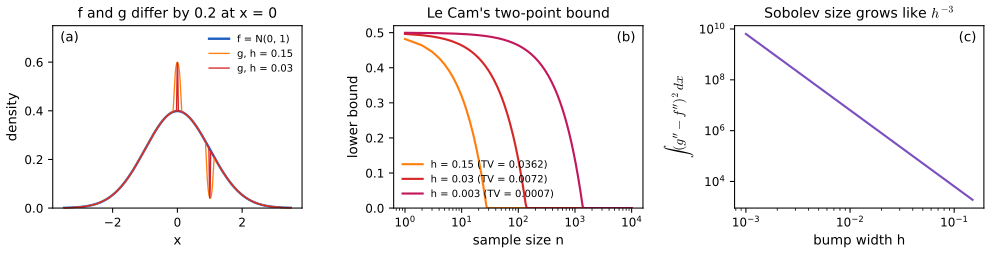
fig_6_s1. Download: PDF · SVGDefinition 6.B (statistical functional) pp. 88–89, Example 6.5
A statistical functional is any function \(T(F)\) of the distribution, for instance the mean \(T(F)=\int x\,\d F(x)\), the variance \(T(F)=\int x^2\,\d F(x)-(\int x\,\d F(x))^2\) and the median \(T(F)=F^{-1}(1/2)\). Estimating \(\mu=\E(X_1)\) assuming only that it exists is the nonparametric problem of estimating a functional.
A functional need not be defined on all of \(\FALL\): the mean is undefined for the Cauchy distribution, which is why Example 6.5 assumes that \(\mu\) exists, and the median \(F^{-1}(1/2)\) needs a convention when \(F\) is flat at level 1/2 (Chapter 2 uses the smallest \(x\) with \(F(x)\ge1/2\)). Filling the gap 6.6 shows that this is not a technicality: for Cauchy data the sample mean is not consistent for anything, while the sample median is consistent for the centre.
p. 89 Example 6.6 (regression, prediction and classification). With pairs \((X_i,Y_i)\), the regression function is \(r(x)=\E(Y\given X=x)\); \(X\) is the predictor (regressor, feature, covariate, independent variable) and \(Y\) the response (outcome, dependent variable). If \(r\) is assumed to lie in a finite-dimensional set (straight lines, say) the regression model is parametric, otherwise nonparametric. Predicting \(Y\) for a new \(X\) is prediction, called classification when \(Y\) is discrete; estimating the whole function \(r\) is regression or curve estimation. Regression models are often written
\[ Y=r(X)+\epsilon,\qquad\E(\epsilon)=0. \tag{6.3} \]Filling the gap 6.3: (6.3) is a definition, not an assumption p. 89
Assume only \(\E|Y|<\infty\). Then \(\epsilon=Y-r(X)\) satisfies \(\E(\epsilon\given X)=0\) (stronger than \(\E\epsilon=0\)), hence \(\E[\epsilon\,h(X)]=0\) for every bounded \(h\). If moreover \(\E Y^2<\infty\), then for every function \(g\) with \(\E g(X)^2<\infty\)
\[ \E\big(Y-g(X)\big)^2=\E\,\epsilon^2+\E\big(r(X)-g(X)\big)^2, \]so \(r\) is the best predictor of \(Y\) in mean squared error.
Proof
\(r(X)\) is a function of \(X\), so \(\E(r(X)\given X)=r(X)\) and \(\E(\epsilon\given X)=\E(Y\given X)-r(X)=0\). The tower property gives \(\E\epsilon=\E\,\E(\epsilon\given X)=0\) and \(\E[\epsilon h(X)]=\E[h(X)\E(\epsilon\given X)]=0\) (taking out what is known). For the last claim write \(Y-g=\epsilon+(r-g)\), square, and take expectations: the cross term \(2\E[\epsilon(r(X)-g(X))]\) vanishes by the same argument (it is finite by Cauchy–Schwarz, since \(\E r(X)^2\le\E Y^2\) by Jensen's inequality for conditional expectations). ∎
So writing a regression as (6.3) restricts nothing. Assumptions enter only when more is asked of \(\epsilon\): independence of \(X\), constant variance, normality. The book's one-line calculation contains a misplaced parenthesis, \(\E(\E(Y-r(X))\given X)\) for \(\E(\E(Y-r(X)\given X))\); see the notes on the book.
See also (companion courses): the regression function as the best predictor, Result 2.3 of Statistical Learning: Theory and Methods; parametric against non-parametric estimates of \(f\), Section 2.1.2 of Applied Statistical Learning.
What comes next, frequentists and Bayesians, notation. p. 89 The book treats nonparametric inference before parametric inference (Chapters 7 and 8 before Chapter 9), and frequentist before Bayesian inference (Chapter 11). For a parametric model, \(\P_\th(X\in A)=\int_Af(x;\th)\,\d x\) and \(\E_\th(r(X))=\int r(x)f(x;\th)\,\d x\); the subscript says which member of the model is used to compute, not that anything is averaged over \(\th\). The two schools differ precisely here: a frequentist statement holds for every fixed \(\th\), while a Bayesian statement averages over a distribution for \(\th\). Filling the gap 6.11 shows how far apart the two can be.
See also (companion course): the frequentist and Bayesian readings of probability, Section 1.2.3 of Bayesian and Probabilistic Machine Learning.
6.3 Fundamental Concepts in Inference
p. 90 Most inferential problems are of one of three kinds: estimation, confidence sets and hypothesis testing. The rest of the book treats each in detail; this section fixes the language.
6.3.1 Point Estimation
Definition 6.C (estimator, bias, standard error, mean squared error) pp. 90–91, (6.4)–(6.6)
Let \(X_1,\dots,X_n\) be iid from a distribution \(F\). A point estimator of a parameter \(\th\) is any function of the data, \(\hth=g(X_1,\dots,X_n)\). Its distribution is the sampling distribution. Its bias, standard error and mean squared error are
\[ \bias(\hth)=\E_\th(\hth)-\th, \tag{6.4} \] \[ \se=\se(\hth)=\sqrt{\V(\hth)}, \tag{6.5} \] \[ \mse=\E_\th(\hth-\th)^2. \tag{6.6} \]\(\hth\) is unbiased if \(\E_\th(\hth)=\th\). When \(\se\) depends on the unknown \(F\), an estimate of it is written \(\hse\).
Keep the roles straight: \(\th\) is fixed and unknown; \(\hth\) is random because it depends on the data. Expectations \(\E_\th\) are taken over the data, with joint density \(f(x_1,\dots,x_n;\th)=\prod_{i=1}^nf(x_i;\th)\), never over \(\th\).
Example 6.8. p. 91 For \(X_i\sim\Bern(p)\) and \(\hp=n^{-1}\sum_iX_i\): \(\E(\hp)=p\), so \(\hp\) is unbiased; \(\se=\sqrt{p(1-p)/n}\); and \(\hse=\sqrt{\hp(1-\hp)/n}\).
Definition 6.7 (consistency) p. 90
A point estimator \(\hth\) of \(\th\) is consistent if \(\hth\convp\th\), that is, if \(\P_\th(|\hth-\th|>\epsilon)\to0\) as \(n\to\infty\) for every \(\epsilon>0\).
Unbiasedness, the book remarks, is less important than it once seemed: many good estimators are biased (Filling the gap 6.4), and some unbiased estimators are poor. Consistency is the minimal requirement that more data should eventually give the right answer.
Theorem 6.9 (bias–variance decomposition) p. 91, (6.7)
If \(\E_\th(\hth^2)<\infty\), then
\[ \mse=\bias^2(\hth)+\V_\th(\hth). \tag{6.7} \]Proof
Let \(\bth=\E_\th(\hth)\), finite by assumption. Write \(\hth-\th=(\hth-\bth)+(\bth-\th)\): a random term with mean zero plus a constant. Squaring,
\[ \E_\th(\hth-\th)^2=\E_\th(\hth-\bth)^2+2(\bth-\th)\,\E_\th(\hth-\bth)+(\bth-\th)^2=\V_\th(\hth)+0+\bias^2(\hth), \]because \(\E_\th(\hth-\bth)=\bth-\bth=0\). The same algebra applied to any distribution, in particular to the empirical distribution of simulated estimates, gives the identity exactly (the Monte Carlo columns of the MSE demo add up for this reason). For a vector parameter, the same steps give \(\E\|\hth-\th\|^2=\|\bias\|^2+\operatorname{trace}\Cov(\hth)\). ∎
See also (companion courses): Theorem 1.1 of the first-year notes; the decomposition of the test error of a regression fit, Result 2.4 of Applied Statistical Learning and Result 7.1 of Statistical Learning: Theory and Methods, which add an irreducible noise term.
Filling the gap 6.4: why "many of the estimators we will use are biased" p. 90
Three families show how bias can buy a lower MSE, and what it costs.
(a) Shrinking a Normal mean. For \(X_i\sim N(\th,\sigma^2)\) and \(\widehat\theta_c=c\overline X_n\),
\[ \mse(c)=(1-c)^2\th^2+c^2\sigma^2/n,\qquad c^*=\frac{\th^2}{\th^2+\sigma^2/n}<1, \]so some shrinkage always beats \(\overline X_n\) (\(c=1\)), but the best amount depends on the unknown \(\th\), and for any fixed \(c<1\), \(\mse(c)\to\infty\) as \(|\th|\to\infty\): no estimator in the family is best for every \(\th\).
(b) Pseudo-counts for a proportion. For \(\widehat p_a=(S+a)/(n+2a)\), \(S\sim\Bin(n,p)\),
\[ \bias=\frac{a(1-2p)}{n+2a},\qquad\V=\frac{np(1-p)}{(n+2a)^2},\qquad a^*(p)=\frac{p(1-p)}{2(p-\frac12)^2}. \]The choice \(a=\sqrt n/2\) makes the MSE constant, equal to \(1/\{4(\sqrt n+1)^2\}\), which is smaller than the worst-case MSE \(1/(4n)\) of \(\hp\) (Hodges and Lehmann, 1950); Chapter 12 shows that it is the minimax estimator.
(c) Rescaling a maximum. For \(X_i\sim\Unif(0,\th)\) and \(c\max_iX_i\), the MSE is minimised by \(c=(n+2)/(n+1)\), not by the unbiased choice \((n+1)/n\) (Exercise 6.2).
Derivations
(a) \(\E\widehat\theta_c=c\th\) and \(\V\widehat\theta_c=c^2\sigma^2/n\); Theorem 6.9 gives \(\mse(c)\), a convex quadratic in \(c\) whose derivative \(-2(1-c)\th^2+2c\sigma^2/n\) vanishes at \(c^*\). Its value there is \(\th^2(\sigma^2/n)/(\th^2+\sigma^2/n)\), less than \(\sigma^2/n\) for every \(\th\).
(b) \(\E\widehat p_a=(np+a)/(n+2a)\), so the bias is \[ \frac{np+a-p(n+2a)}{n+2a}=\frac{a(1-2p)}{n+2a}, \] and \(\V\widehat p_a=\V S/(n+2a)^2\). Hence
\[ \mse(a)=\frac{a^2(1-2p)^2+np(1-p)}{(n+2a)^2}. \]Setting the derivative in \(a\) to zero and cancelling \(4a^2(1-2p)^2\) on both sides:
\[ \begin{aligned} 2a(1-2p)^2(n+2a)&=4\{a^2(1-2p)^2+np(1-p)\},\\ 2an(1-2p)^2&=4np(1-p),\\ a^*&=\frac{2p(1-p)}{(1-2p)^2}=\frac{p(1-p)}{2(p-\frac12)^2}. \end{aligned} \]For the constant-risk choice, write \((1-2p)^2=1-4p(1-p)\) and \(q=p(1-p)\): the numerator is \(a^2+q(n-4a^2)\), free of \(p\) exactly when \(4a^2=n\); then \[ \mse=\frac{a^2}{(n+2a)^2}=\frac{n}{4(n+\sqrt n)^2}=\frac{1}{4(\sqrt n+1)^2}. \] With \(n=20\) this is 0.0083 against the MLE's worst case 0.0125.
(c) With \(M=\max_iX_i\): \(\E M=n\th/(n+1)\) and \(\E M^2=n\th^2/(n+2)\) (Exercise 6.2 below), so \[ \mse(c)=\frac{c^2n\th^2}{n+2}-\frac{2cn\th^2}{n+1}+\th^2, \] minimised at \(c=(n+2)/(n+1)\) with value \(\th^2/(n+1)^2\), slightly below the unbiased estimator's \(\th^2/\{n(n+2)\}\). ∎
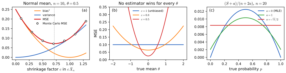
fig_6_s2. Download: PDF · SVGTheorem 6.10 (bias and se tending to zero imply consistency) p. 91
If \(\bias(\hth)\to0\) and \(\se(\hth)\to0\) as \(n\to\infty\), then \(\hth\convp\th\).
Proof
By Theorem 6.9, \(\mse=\bias^2+\se^2\to0\), which is convergence in quadratic mean (Definition 5.2 of the book). Quadratic-mean convergence implies convergence in probability (part (a) of Theorem 5.4 of the book; the printed proof says part (b), a slip listed in the author's errata). Directly: by Markov's inequality applied to the nonnegative variable \((\hth-\th)^2\),
\[ \P_\th\big(|\hth-\th|>\epsilon\big)\le\P_\th\big((\hth-\th)^2\ge\epsilon^2\big)\le\frac{\E_\th(\hth-\th)^2}{\epsilon^2}=\frac{\mse}{\epsilon^2}\to0 \]for every \(\epsilon>0\). ∎
See also (companion course): Theorem 1.2 of the first-year notes.
Example 6.11. p. 91 For coin flips, \(\bias(\hp)=0\) and \(\se=\sqrt{p(1-p)/n}\to0\), so \(\hp\) is consistent. Figure 6.S3(b) compares the exact probability \(\P(|\hp-p|>\epsilon)\) with the Chebyshev bound \(\mse/\epsilon^2\) used in the proof and with Hoeffding's bound: for \(p=0.3\), \(\epsilon=0.05\) and \(n=1000\) the three are 0.00049, 0.084 and 0.013.
Filling the gap 6.5: the condition of Theorem 6.10 is sufficient, not necessary p. 91
(a) \(\mse\to0\) holds if and only if both \(\bias\to0\) and \(\se\to0\). (b) A consistent estimator can have a bias that does not tend to 0 and an MSE that tends to infinity.
Proof
(a) By (6.7) the MSE is a sum of two nonnegative terms; it tends to 0 if and only if each does.
(b) Let \(B_n\sim\Bern(1/n)\) be independent of the data, and let \(\hth=\overline X_n+nB_n\) for data with mean \(\th\) and variance \(\sigma^2\). Then
\[ \P(|\hth-\th|>\epsilon)\le\P(|\overline X_n-\th|>\epsilon)+\P(B_n=1)\le\frac{\sigma^2}{n\epsilon^2}+\frac1n\to0, \]so \(\hth\) is consistent; yet \(\E\hth-\th=n\cdot\frac1n=1\) for every \(n\), and \[ \mse\ge\V(nB_n)=n^2\cdot\tfrac1n\big(1-\tfrac1n\big)=n-1\to\infty. \] The rare large error has probability \(1/n\to0\), which consistency ignores, but its size \(n\) dominates every moment. A more natural example, with no artificial noise, is the sample median of Cauchy data in the next box: consistent, though for \(n\le2\) its variance is infinite and the mean of the data does not exist. ∎
Filling the gap 6.6: the Cauchy mean never settles; the Cauchy median does pp. 88–91
Let \(X_i\) be iid standard Cauchy, with density \(1/\{\pi(1+x^2)\}\) and centre (median) 0. (a) For every \(n\), \(\overline X_n\) is again standard Cauchy, so \(\P(|\overline X_n|>\epsilon)=1-\tfrac2\pi\arctan\epsilon\) does not depend on \(n\): \(\overline X_n\) is not consistent for 0, nor for any other constant. (b) The sample median \(M_n=X_{(\lceil n/2\rceil)}\) is consistent for 0, with
\[ \P(|M_n|>\epsilon)\le e^{-2n\delta_n^2}+e^{-2n\delta^2},\qquad\delta=\tfrac1\pi\arctan\epsilon,\ \ \delta_n=\delta-\tfrac1{2n}, \]for \(n>1/(2\delta)\). More generally, the sample median is consistent for the median \(m\) of any \(F\) that is strictly increasing at \(m\).
Proof
(a) The characteristic function of the standard Cauchy is \(\varphi(t)=e^{-|t|}\). By independence, \(\E e^{it\overline X_n}=\varphi(t/n)^n=e^{-n|t|/n}=e^{-|t|}\), and the characteristic function determines the distribution. If \(\overline X_n\convp c\) for some constant \(c\), then \(\overline X_n\convd c\), impossible since the law of \(\overline X_n\) is the same non-degenerate law for all \(n\).
(b) Let \(k=\lceil n/2\rceil\), so \(k\le(n+1)/2\). The event \(\{M_n>m+\epsilon\}\) means that fewer than \(k\) observations are at most \(m+\epsilon\). The count \(N=\#\{i:X_i\le m+\epsilon\}\) is \(\Bin(n,q)\) with \(q=F(m+\epsilon)\), and \(q>1/2\) because \(F\) is strictly increasing at \(m\). Hence
\[ \P(M_n>m+\epsilon)=\P(N<k)\le\P\Big(\frac Nn-q\le\frac12+\frac1{2n}-q\Big)\le e^{-2n(q-\frac12-\frac1{2n})^2} \]by Hoeffding's inequality (Theorem 4.4 of the book) once \(q-\frac12>\frac1{2n}\). Symmetrically, \(\{M_n<m-\epsilon\}\) means that at least \(k\ge n/2\) observations are below \(m-\epsilon\); that count is \(\Bin(n,q')\) with \(q'=F(m-\epsilon)<1/2\), and \(\P\le e^{-2n(\frac12-q')^2}\). For the Cauchy, \(q-\frac12=\frac12-q'=\frac1\pi\arctan\epsilon=\delta\). Both bounds tend to 0, so \(M_n\convp m\), and exponentially fast. The exact probability used in the demonstration is \[ \P(M_n\le x)=\P\big(\Bin(n,F(x))\ge k\big)=I_{F(x)}(k,n-k+1), \] with \(I\) the regularised incomplete beta function. ∎
The median is also asymptotically Normal, \(\sqrt n(M_n-m)\convd N(0,1/\{4f(m)^2\})\) (van der Vaart, 1998, Section 21.2), which for the Cauchy is \(N(0,\pi^2/4)\). At \(n=101\) and \(\epsilon=0.1\) the Normal approximation gives \(\P(|M_n|>0.1)\approx0.5223\), against the exact 0.5222.
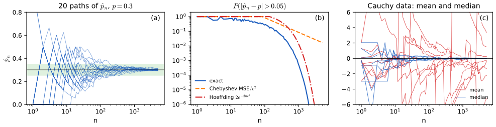
fig_6_s3. Download: PDF · SVGpp. 91–92 Many estimators have, approximately, a Normal sampling distribution.
Definition 6.12 (asymptotic normality) p. 92, (6.8)
An estimator is asymptotically Normal if
\[ \frac{\hth-\th}{\se}\convd N(0,1). \tag{6.8} \]In practice \(\se\) is unknown and is replaced by \(\hse\), and Theorem 6.16 below assumes the version with \(\hse\). The bridge between the two is the next box.
Filling the gap 6.7: replacing \(\se\) by \(\hse\) pp. 92–94
If \((\hth-\th)/\se\convd N(0,1)\) and \(\hse/\se\convp1\), then \((\hth-\th)/\hse\convd N(0,1)\). For \(\Bern(p)\) data with \(0<p<1\), \(\hp\) satisfies both conditions with \(\hse=\sqrt{\hp(1-\hp)/n}\).
Proof
Write \(Z_n=(\hth-\th)/\se\), \(R_n=\hse/\se\) and \(Z_n/R_n=Z_n+V_n\) with \(V_n=Z_n(1/R_n-1)\).
Step 1: \(V_n\convp0\). Fix \(\eta,\delta>0\) and choose \(K\) with \(\P(|Z|>K)<\eta\) for \(Z\sim N(0,1)\). Since \(\Phi\) is continuous, \(\P(|Z_n|>K)\to\P(|Z|>K)\), so \(\P(|Z_n|>K)<2\eta\) for large \(n\). Also \(1/R_n-1\convp0\), because \(x\mapsto1/x-1\) is continuous at 1 (Theorem 5.5(f) of the book). Then, for large \(n\), \[ \P(|V_n|>\delta)\le\P(|Z_n|>K)+\P(|1/R_n-1|>\delta/K)<3\eta. \]
Step 2: a small perturbation does not change the limit. For every \(x\) and \(\delta>0\), \[ \{Z_n+V_n\le x\}\subset\{Z_n\le x+\delta\}\cup\{|V_n|>\delta\}, \] so \(\limsup\P(Z_n+V_n\le x)\le\Phi(x+\delta)\); similarly \[ \{Z_n\le x-\delta\}\subset\{Z_n+V_n\le x\}\cup\{|V_n|>\delta\} \] gives \(\liminf\P(Z_n+V_n\le x)\ge\Phi(x-\delta)\). Letting \(\delta\to0\) and using the continuity of \(\Phi\), \(\P(Z_n/R_n\le x)\to\Phi(x)\). (This is Slutsky's theorem, Theorem 5.5(c) and (e) of the book, in the case needed here.)
Bernoulli. The central limit theorem gives \((\hp-p)/\sqrt{p(1-p)/n}\convd N(0,1)\). By the weak law of large numbers \(\hp\convp p\), and \(x\mapsto\sqrt{x(1-x)/(p(1-p))}\) is continuous at \(p\) with value 1 there, so \(\hse/\se\convp1\). At \(p\in\{0,1\}\) both conditions fail: \(\se=0\) and the data are constant. ∎
6.3.2 Confidence Sets
Definition 6.D (confidence interval, coverage) p. 92, (6.9)
A \(1-\alpha\) confidence interval for \(\th\) is a random interval \(C_n=(a,b)\), with endpoints \(a=a(X_1,\dots,X_n)\) and \(b=b(X_1,\dots,X_n)\) computed from the data, such that
\[ \P_\th(\th\in C_n)\ge1-\alpha\quad\text{for all }\th\in\Theta. \tag{6.9} \]The number \(1-\alpha\) is the coverage. For a vector \(\th\) the interval is replaced by a confidence set (a ball, an ellipsoid).
Two warnings from the book. First, \(C_n\) is random and \(\th\) is fixed: the probability in (6.9) is over the data. Second, a confidence interval is not a probability statement about \(\th\). The usual reading, "if the experiment were repeated many times, 95% of the intervals would contain \(\th\)", is correct but rarely relevant, since experiments are rarely repeated. The book's better reading: day after day you build 95% intervals for unrelated parameters \(\th_1,\th_2,\dots\), and in the long run 95% of them trap their parameter. This deserves a proof.
Filling the gap 6.8: the "unrelated parameters" reading is a theorem p. 92
On day \(j\) a \(1-\alpha\) interval \(C^{(j)}\) is built for a parameter \(\th_j\) from data independent of the other days, and \(I_j=1\{\th_j\in C^{(j)}\}\). If each interval satisfies (6.9), then with probability one
\[ \liminf_{m\to\infty}\frac1m\sum_{j=1}^mI_j\ \ge\ 1-\alpha, \]with equality in the limit when every coverage is exactly \(1-\alpha\). The parameters, the models and the sample sizes may all change from day to day.
Proof
The \(I_j\) are independent Bernoulli variables with means \(c_j=\P_{\th_j}(\th_j\in C^{(j)})\ge1-\alpha\). They are not identically distributed, so the ordinary law of large numbers does not apply directly, but Hoeffding's inequality (Theorem 4.4 of the book, which allows different bounded variables) does: with \(Y_j=I_j-c_j\in[-c_j,1-c_j]\), an interval of length 1,
\[ \P\Big(\frac1m\sum_{j=1}^m(I_j-c_j)<-\eta\Big)\le e^{-2m\eta^2}. \]The right side is summable in \(m\), so by the Borel–Cantelli lemma, with probability one only finitely many \(m\) have \(\frac1m\sum_j(I_j-c_j)<-\eta\). On that event \[ \liminf_m\frac1m\sum_jI_j\ \ge\ \liminf_m\frac1m\sum_jc_j-\eta\ \ge\ 1-\alpha-\eta. \] Taking \(\eta=1/k\) and intersecting the countably many probability-one events over \(k\) gives the claim; the same argument for the upper tail gives the limit \(1-\alpha\) when all \(c_j=1-\alpha\). ∎
Two remarks. Independence across days is used (a martingale version of Hoeffding's inequality, Azuma's, would allow the choice of each day's problem to depend on the past). And the guarantee is only as good as (6.9): for approximate intervals the long-run fraction is the average of the actual coverages \(c_j\), which can be well below \(1-\alpha\) (Figure 6.S5(a), where Wald intervals for polls of size 30 trap their parameter 90% of the time).
See also (companion course): the frequency meaning of "95%", Theorem 3.2 of the first-year notes, and its confidence-interval demo.
Example 6.13 (opinion polls). pp. 92–93 A poll reports that 83% of the population favour a proposal, "accurate to within 4 points 95 percent of the time". That is a 95% confidence interval \(83\pm4\) for the unknown proportion; by Filling the gap 6.8, a reader who forms such intervals for a different question every day traps the truth 95% of the time in the long run.
Filling the gap 6.9: where "within 4 points" comes from p. 93
The Normal-based interval of Example 6.17 has half-width \(z_{\alpha/2}\sqrt{\hp(1-\hp)/n}\). Pollsters usually quote the worst case \(\hp=1/2\), the margin \(1.96/(2\sqrt n)\approx1/\sqrt n\), which equals 0.04 at \(n=601\) (with 1.96) or 625 (with the rounding \(1.96\approx2\)). At \(\hp=0.83\) the same margin needs only \(n=339\), and a poll of 1000 people gives \(\pm2.3\) points.
Derivation
Solve \(z\sqrt{q/n}=0.04\) for \(n\): \(n=z^2q/0.04^2\). With \(z=1.96\): \(q=0.25\) gives \(n=600.2\), so 601; \(q=0.83\times0.17=0.1411\) gives \(n=338.8\), so 339. With \(n=1000\) and \(\hp=0.83\), \(1.96\sqrt{0.1411/1000}=0.0233\). ∎
Example 6.14 (a 75% interval that is certainly right). p. 93 This example, which the book takes from Berger and Wolpert (1984), sharpens the second warning. Let \(\th\) be a fixed, unknown real number (the book prints "known", see the notes on the book), let \(X_1,X_2\) be independent with \(\P(X_i=1)=\P(X_i=-1)=1/2\), and observe only \(Y_i=\th+X_i\). Define the one-point "interval"
\[ C=\begin{cases}\{Y_1-1\}&\text{if }Y_1=Y_2,\\ \{(Y_1+Y_2)/2\}&\text{if }Y_1\ne Y_2.\end{cases} \]Then \(\P_\th(\th\in C)=3/4\) for every \(\th\), so \(C\) is a 75% confidence set. Yet if we observe \(Y_1=15\), \(Y_2=17\), then \(C=\{16\}\) and we are certain that \(\th=16\).
Filling the gap 6.10: "you can check" that the coverage is 3/4 p. 93
Overall coverage is 3/4; conditionally on \(Y_1\ne Y_2\) it is 1, and conditionally on \(Y_1=Y_2\) it is 1/2.
Proof
The four outcomes of \((X_1,X_2)\) are equally likely. If \(X_1\ne X_2\) (probability 1/2), the observations are \(\th-1\) and \(\th+1\) in some order, their average is \(\th\), and \(C\) traps \(\th\). If \(X_1=X_2=1\) (probability 1/4), \(Y_1-1=\th\): trapped. If \(X_1=X_2=-1\) (probability 1/4), \(Y_1-1=\th-2\): missed. Total \(1/2+1/4=3/4\), whatever \(\th\) is. Conditionally on \(Y_1\ne Y_2\) the coverage is 1, and on \(Y_1=Y_2\) it is \((1/4)/(1/2)=1/2\). ∎
So the 75% is an average over two kinds of data sets that are told apart by the data themselves; it describes the procedure, not the interval in hand. Statistics that are uninformative about \(\th\) but tell us how precise the data happen to be (here, whether \(Y_1=Y_2\)) are called ancillary, and conditioning on them is a recurring theme of the foundations of inference (Berger and Wolpert, 1984).
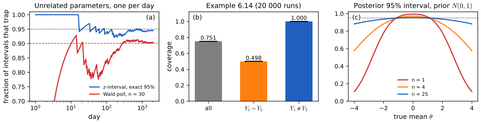
fig_6_s5. Download: PDF · SVGp. 93 Chapter 11 introduces Bayesian intervals, which do make probability statements about \(\th\) ("given the data, \(\th\) is in \(C_n\) with probability 95%"), but these are degrees of belief and, the book says, need not trap the parameter 95% of the time. Here is how far from 95% they can be.
Filling the gap 6.11: the frequentist coverage of a Bayesian interval p. 93
Let \(X_1,\dots,X_n\sim N(\th,\sigma^2)\) with \(\sigma\) known, give \(\th\) the prior \(N(0,\tau^2)\), and let \(s^2=\sigma^2/n\) and \(w=\tau^2/(\tau^2+s^2)\). The posterior is \(N(w\overline X_n,ws^2)\), and the 95% posterior interval \(w\overline X_n\pm z_{\alpha/2}\sqrt w\,s\) has frequentist coverage
\[ \P_\th(\th\in C_n)=\Phi\Big(\frac{z_{\alpha/2}}{\sqrt w}+\delta\Big)-\Phi\Big(-\frac{z_{\alpha/2}}{\sqrt w}+\delta\Big),\qquad\delta=\frac{(1-w)\th}{ws}. \]It exceeds \(1-\alpha\) at \(\th=0\), tends to 0 as \(|\th|\to\infty\), and its average over the prior is exactly \(1-\alpha\).
Proof
Posterior. As a function of \(\th\), the likelihood is proportional to \(\exp\{-(\overline X_n-\th)^2/(2s^2)\}\) and the prior to \(\exp\{-\th^2/(2\tau^2)\}\). Completing the square in \(\th\): the precision is \(1/s^2+1/\tau^2=1/(ws^2)\) and the mean is \(ws^2\cdot\overline X_n/s^2=w\overline X_n\).
Coverage. For fixed \(\th\), \(w\overline X_n\sim N(w\th,w^2s^2)\). The event \(|w\overline X_n-\th|<z\sqrt ws\) is, after standardising \(U=(w\overline X_n-w\th)/(ws)\sim N(0,1)\), the event \(|U-\delta|<z/\sqrt w\) with \(\delta=(1-w)\th/(ws)\), whose probability is the display. At \(\th=0\) it is \(2\Phi(z/\sqrt w)-1>1-\alpha\) since \(w<1\); as \(|\th|\to\infty\), \(|\delta|\to\infty\) and the probability tends to 0.
Average over the prior. Under the joint distribution of \((\th,X)\), \(\P(\th\in C_n)=\E[\P(\th\in C_n\given X)]=1-\alpha\), because given the data \(C_n\) has posterior probability \(1-\alpha\) by construction; and also \(\P(\th\in C_n)=\E[\P_\th(\th\in C_n)]\), the prior average of the coverage function. ∎
With \(\tau=\sigma=1\) and \(n=1\) (\(w=1/2\)): coverage 0.994 at \(\th=0\), 0.78 at \(\th=2\), 0.41 at \(\th=3\). With \(n=25\) the prior matters little and the coverage stays above 0.91 for \(|\th|\le3\). A Bayesian interval is a frequentist 95% interval "on average over the prior", which is the guarantee (6.9) only when the prior is right.
Example 6.15 (an interval from Hoeffding's inequality). p. 93 For coin flips, let \(C_n=(\hp-\epsilon_n,\hp+\epsilon_n)\) with \(\epsilon_n^2=\log(2/\alpha)/(2n)\). Then \(\P(p\in C_n)\ge1-\alpha\) for every \(p\) and every \(n\): an exact, finite-sample confidence interval.
Filling the gap 6.12: the Hoeffding interval, and the price of its guarantee pp. 93–94
(a) \(\P_p(|\hp-p|\ge\epsilon)\le2e^{-2n\epsilon^2}\) for every \(p\), \(n\) and \(\epsilon>0\), so \(C_n\) satisfies (6.9). (b) Whatever the data, the Hoeffding interval is wider than the Normal-based interval of Example 6.17 by at least the factor \(\sqrt{2\log(2/\alpha)}/z_{\alpha/2}>1\), which is 1.488, 1.386 and 1.264 for 90%, 95% and 99% intervals.
Proof
(a) For \(t>0\), Markov's inequality applied to \(e^{t\sum_i(X_i-p)}\) gives
\[ \P(\hp-p\ge\epsilon)\le e^{-tn\epsilon}\prod_{i=1}^n\E e^{t(X_i-p)}\le e^{-tn\epsilon+nt^2/8}, \]using Hoeffding's lemma \(\E e^{tY}\le e^{t^2(b-a)^2/8}\) for a mean-zero \(Y\in[a,b]\), here with \(b-a=1\) (this is the bound (4.3) in Theorem 4.4 of the book, proved in the appendix of its Chapter 4). Choosing \(t=4\epsilon\) gives \(e^{-2n\epsilon^2}\); the lower tail is the same with \(-X_i\). Note the non-strict \(\ge\): since \(C_n\) is open, \(p\notin C_n\) means \(|\hp-p|\ge\epsilon_n\), and it is this version, which the Chernoff argument provides, that is needed (the book's (4.4) is stated with \(>\)). Setting \(2e^{-2n\epsilon^2}=\alpha\) gives \(\epsilon_n\).
(b) Since \(\hp(1-\hp)\le1/4\), the Normal-based half-width is at most \(z_{\alpha/2}/(2\sqrt n)\), while the Hoeffding half-width is \(\sqrt{\log(2/\alpha)/(2n)}\). Their ratio is at least \(\sqrt{2\log(2/\alpha)}/z_{\alpha/2}\). This exceeds 1 if and only if \(\alpha<2e^{-z^2/2}\) with \(z=z_{\alpha/2}\), that is \(1-\Phi(z)<e^{-z^2/2}\), which is the Chernoff bound for the Normal tail (Mill's inequality, Theorem 4.7 of the book, gives a similar bound): \(1-\Phi(z)\le e^{-tz}\E e^{tZ}=e^{-tz+t^2/2}\), minimised at \(t=z\). ∎
The guarantee is paid for twice: the interval ignores that \(\V(\hp)=p(1-p)/n\) is small when \(p\) is near 0 or 1, and Hoeffding's lemma is tight only for the worst case. Its exact coverage is above 99.3% for every \(p\) when \(n=50\) (Figure 6.S4), far above the promised 95%.
See also (this course): the Chapter 4 Hoeffding-interval demo, built on the inequality itself.
pp. 93–94 When the estimator is asymptotically Normal, (6.8) suggests \(\hth\approx N(\th,\hse^2)\), and an approximate interval follows.
Theorem 6.16 (Normal-based confidence interval) p. 94, (6.10)–(6.11)
Suppose \((\hth-\th)/\hse\convd N(0,1)\). Let \(z_{\alpha/2}=\Phi^{-1}(1-\alpha/2)\), so that \(\P(-z_{\alpha/2}<Z<z_{\alpha/2})=1-\alpha\) for \(Z\sim N(0,1)\), and
\[ C_n=\big(\hth-z_{\alpha/2}\,\hse,\ \hth+z_{\alpha/2}\,\hse\big). \tag{6.10} \]Then
\[ \P_\th(\th\in C_n)\to1-\alpha. \tag{6.11} \]Proof
Let \(Z_n=(\hth-\th)/\hse\) and \(G_n\) its cdf. Since \(\hse>0\), \(\th\in C_n\) if and only if \(-z<Z_n<z\) with \(z=z_{\alpha/2}\), so \(\P_\th(\th\in C_n)=\P(Z_n<z)-G_n(-z)\). Convergence in distribution gives \(G_n(x)\to\Phi(x)\) at every \(x\), since \(\Phi\) is continuous everywhere; so \(G_n(-z)\to\Phi(-z)\). The book's proof stops here, but \(\P(Z_n<z)\) is a left limit \(G_n(z^-)\), not \(G_n(z)\), and needs one more step: for \(\delta>0\), \(G_n(z-\delta)\le\P(Z_n<z)\le G_n(z)\), so \[ \Phi(z-\delta)\le\liminf_n\P(Z_n<z)\le\limsup_n\P(Z_n<z)\le\Phi(z); \] letting \(\delta\to0\), \(\P(Z_n<z)\to\Phi(z)\). Hence the coverage tends to \(\Phi(z)-\Phi(-z)=1-\alpha\). The assumption is the one with \(\hse\); Filling the gap 6.7 derives it from (6.8). ∎
For 95% intervals \(z_{0.025}=1.96\approx2\), whence the familiar \(\hth\pm2\,\hse\). Note what (6.11) does not say: it is a limit for each fixed \(\th\), with no rate and no uniformity in \(\th\), so for a given \(n\) the coverage can be far from \(1-\alpha\) at some \(\th\) (Section 6.5).
See also (companion course): large-sample intervals for a mean, Theorem 3.5 of the first-year notes, and for proportions, Theorem 3.9.
Example 6.17 (the Wald interval for a proportion). p. 94 For \(\Bern(p)\) data, \(\V(\hp)=n^{-2}\sum_i\V(X_i)=p(1-p)/n\), so \(\se=\sqrt{p(1-p)/n}\) and \(\hse=\sqrt{\hp(1-\hp)/n}\). By the central limit theorem and Filling the gap 6.7, an approximate \(1-\alpha\) interval is
\[ \hp\pm z_{\alpha/2}\,\hse=\hp\pm z_{\alpha/2}\sqrt{\frac{\hp(1-\hp)}{n}}. \]It is shorter than the Hoeffding interval of Example 6.15 (Filling the gap 6.12), but its coverage is only approximately correct, for large samples. Because \(S=n\hp\) takes only \(n+1\) values, the coverage can be computed exactly, and it behaves worse than "approximately 95%" suggests.
Filling the gap 6.13: the exact coverage of the Wald interval, and why it oscillates p. 94
Let \((L_k,U_k)\) be the interval computed from \(S=k\). Then
\[ \P_p(p\in C_n)=\sum_{k=0}^n\binom nk p^k(1-p)^{n-k}\,1\{L_k<p<U_k\}. \](a) As a function of \(p\), the coverage is a polynomial between consecutive endpoints and jumps by a whole binomial term \(\binom nkp^k(1-p)^{n-k}\) at each endpoint. (b) As a function of \(n\) with \(p\) fixed, the set of \(k\) that trap \(p\) is an integer interval whose ends move by whole units, so the coverage oscillates around its limit by amounts of order \(1/\sqrt n\) rather than settling monotonically. (c) Near the edges the Wald coverage collapses: it is at most \(1-(1-p)^n\), which tends to 0 as \(p\to0\).
Proof and numbers
The display is the law of total probability over the values of \(S\). (a) The indicator \(1\{L_k<p<U_k\}\) changes only when \(p\) crosses one of the \(2(n+1)\) endpoints; between them the coverage is a fixed sum of the polynomials \(\binom nkp^k(1-p)^{n-k}\). (b) For the Wald interval, \(L_k<p<U_k\) means \(|k-np|<z\sqrt{k(n-k)/n}\), a condition satisfied by the integers \(k\) in an interval \([a_n,b_n]\). The coverage is \(\P(a_n\le S\le b_n)\). The endpoints \(a_n,b_n\) are integers while the "ideal" endpoints are not, so each end gains or loses a fraction of a binomial term as \(n\) changes, and a single term is of order \(1/\sqrt{2\pi np(1-p)}\) near the centre of the distribution: this is the size of the oscillation (Brown, Cai and DasGupta, 2001, analyse it in detail). (c) If \(S=0\) then \(\hp=0\), \(\hse=0\) and the interval is the empty open interval \((0,0)\) (or the point \(\{0\}\) if closed); either way it misses every \(p>0\). So the coverage is at most \(1-\P(S=0)=1-(1-p)^n\). ∎
Numbers (exact, Figure 6.S4): with \(p=0.2\) the 95% Wald coverage is 0.815 at \(n=15\), 0.871 at \(n=17\), 0.921 at \(n=20\), then 0.905 at \(n=40\) and 0.929 at \(n=42\); over \(10\le n\le200\) it never exceeds 0.954. With \(n=50\), averaged over a fine grid of \(p\), it is 0.90; the Wilson interval, which inverts the test \(|\hp-p|\le z\sqrt{p(1-p)/n}\) instead of plugging in \(\hp\) (Wilson, 1927), averages 0.952 and the Hoeffding interval 0.998.
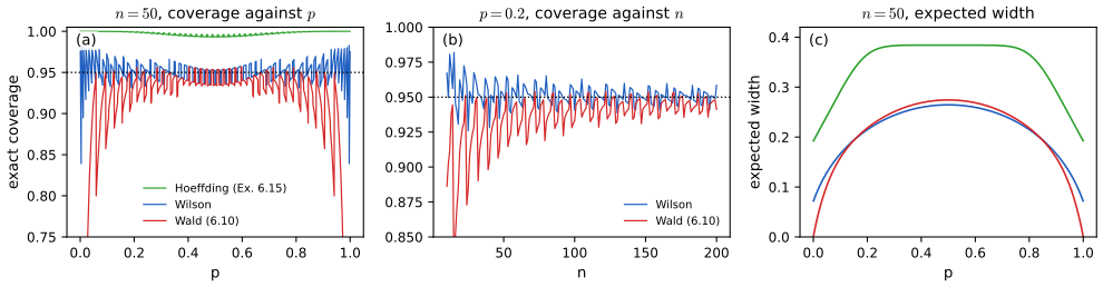
fig_6_s4. Download: PDF · SVG6.3.3 Hypothesis Testing
pp. 94–95 In hypothesis testing we start from a default theory, the null hypothesis, and ask whether the data give enough evidence to reject it; if not, we retain it (other books say "accept" or "fail to reject"; the book's term avoids suggesting that the null has been shown to be true).
Definition 6.E (null and alternative hypotheses) p. 95, Example 6.18
Within a model with parameter space \(\Theta\), a hypothesis is a subset of \(\Theta\) (the dictionary of Section 6.1). The null hypothesis \(H_0:\th\in\Theta_0\) is tested against the alternative hypothesis \(H_1:\th\in\Theta_1=\Theta\setminus\Theta_0\). For a fair coin, \(H_0:p=1/2\) against \(H_1:p\ne1/2\).
Example 6.18 (is the coin fair?). p. 95 With \(n\) independent flips it is natural to reject \(H_0:p=1/2\) when \(T=|\hp-\tfrac12|\) is large. The book postpones "how large" to Chapter 10; the next box gives the answer this chapter's tools already provide.
Filling the gap 6.14: how large must \(T\) be? p. 95
Reject \(H_0\) when \(T>z_{\alpha/2}/(2\sqrt n)\). Under \(H_0\) the probability of rejecting (the size, or type I error rate) tends to \(\alpha\). Equivalently: reject exactly when \(1/2\) lies outside the Wald-type interval \(\hp\pm z_{\alpha/2}\se_0\) with the null standard error \(\se_0=1/(2\sqrt n)\). The exact sizes of the 5% test are 0.041 (\(n=20\)), 0.065 (\(n=50\)), 0.057 (\(n=100\)) and 0.054 (\(n=1000\)).
Proof
Under \(H_0\), \(\V(\hp)=1/(4n)\) is known, and by the central limit theorem \(Z_n=(\hp-\frac12)/\se_0\convd N(0,1)\). The test rejects when \(|Z_n|>z_{\alpha/2}\), and \(\P_{1/2}(|Z_n|>z_{\alpha/2})\to\P(|Z|>z_{\alpha/2})=\alpha\) by the argument in the proof of Theorem 6.16. The exact size is \(\sum_k\binom nk2^{-n}1\{|k/n-\frac12|>z_{\alpha/2}/(2\sqrt n)\}\), which is not monotone in \(n\) for the lattice reason of Filling the gap 6.13. Testing and interval estimation are two sides of one coin: a test of \(\th=\th_0\) at level \(\alpha\) can be built by rejecting when \(\th_0\) is outside a \(1-\alpha\) confidence interval, and conversely the set of \(\th_0\) not rejected is a confidence set (Chapter 10). ∎
See also (companion course): the logic of tests and P-values, Section 4 of the first-year notes; in this course, Chapter 10 (see the course home).
6.4 Bibliographic Remarks
p. 95 The book recommends, for elementary reading, DeGroot and Schervish (2002) and Larsen and Marx (1986); at the intermediate level, Casella and Berger (2002), Bickel and Doksum (2000) and Rice (1995); at the advanced level, Cox and Hinkley (2000), Lehmann and Casella (1998), Lehmann (1986) and van der Vaart (1998). For the topics of the gaps filled above: the two-point method of Filling the gap 6.2 goes back to Le Cam (1973) and is developed in Tsybakov (2009); the coverage of intervals for a proportion is surveyed by Brown, Cai and DasGupta (2001), who also discuss the Wilson (1927) and Agresti and Coull (1998) intervals; the constant-risk estimator of a proportion is due to Hodges and Lehmann (1950); the conditionality issues of Example 6.14 are discussed at length by Berger and Wolpert (1984).
6.5 Appendix
Definition 6.F (pointwise and uniform asymptotic coverage) p. 95
Definition 6.D requires \(\P_\th(\th\in C_n)\ge1-\alpha\) for all \(\th\) and all \(n\). A pointwise asymptotic \(1-\alpha\) interval requires only
\[ \liminf_{n\to\infty}\P_\th(\th\in C_n)\ge1-\alpha\quad\text{for every }\th\in\Theta, \]and a uniform asymptotic \(1-\alpha\) interval requires
\[ \liminf_{n\to\infty}\ \inf_{\th\in\Theta}\P_\th(\th\in C_n)\ge1-\alpha. \]The book notes that the Normal-based interval is a pointwise asymptotic interval.
The difference matters in practice: with a uniform guarantee one sample size \(n\) works for all parameter values; with only a pointwise one, the \(n\) needed for coverage close to \(1-\alpha\) depends on the unknown parameter, and may be arbitrarily large.
Filling the gap 6.15: the Wald interval is pointwise but not uniform p. 95
On \(\Theta=(0,1)\): (a) the Wald interval is a pointwise asymptotic \(1-\alpha\) interval; (b) for every \(n\), \(\inf_{0<p<1}\P_p(p\in C_n)=0\), so it is not uniform; (c) more precisely, at \(p=\lambda/n\) the coverage converges, as \(n\to\infty\), to a limit that depends on \(\lambda\) and is below \(1-\alpha\) (about 0.095 for \(\lambda=0.1\)); (d) the Hoeffding interval is uniform, and even satisfies (6.9) for every \(n\).
Proof
(a) For fixed \(p\in(0,1)\) this is Theorem 6.16 combined with Filling the gap 6.7.
(b) By Filling the gap 6.13(c), \(\P_p(p\in C_n)\le1-(1-p)^n\), which tends to 0 as \(p\downarrow0\) for each fixed \(n\).
(c) With \(p=\lambda/n\), \(S\) converges in distribution to Poisson(\(\lambda\)) (Chapter 2 of the book). For \(S=k\ge1\) fixed, the Wald interval is \(k/n\pm z\sqrt{k(1-k/n)}/n\), so \(p=\lambda/n\) lies inside exactly when \(|k-\lambda|<z\sqrt{k(1-k/n)}\), which tends to the condition \(|k-\lambda|<z\sqrt k\); \(S=0\) never covers. Hence the coverage tends to \(\sum_{k\ge1}e^{-\lambda}\lambda^k/k!\,1\{|k-\lambda|<z\sqrt k\}\), a Poisson probability that is not \(1-\alpha\) in general; for \(\lambda=0.1\) and \(z=1.96\) all \(k=1,\dots,4\) qualify and the limit is about \(1-e^{-0.1}=0.095\). The exact coverage at \(p=0.1/n\) is 0.0955 for \(n=10\) and 0.0952 for \(n=50\), \(100\), \(1000\) and \(10\,000\): no sample size helps when \(p\) shrinks with \(n\).
(d) Filling the gap 6.12(a) gives \(\P_p(p\in C_n)\ge1-\alpha\) for every \(p\) and \(n\), so the infimum over \(p\) is at least \(1-\alpha\) for every \(n\). ∎
On the grid \(p=0.001,\dots,0.999\) the lowest 95% Wald coverage is 0.020 (\(n=20\)), 0.049 (\(n=50\)), 0.095 (\(n=100\)) and 0.39 (\(n=500\)), attained at \(p=0.001\); the Wilson interval is not uniform either, but its lowest coverage on the same grid is 0.85, 0.86, 0.90 and 0.91; the Hoeffding interval's is never below 0.993. The Normal-mean interval \(\overline X_n\pm z_{\alpha/2}\sigma/\sqrt n\) with known \(\sigma\) has coverage exactly \(1-\alpha\) for every \(\mu\) and \(n\), the ideal case.
Notes on the book
Two slips of Chapter 6 are in the author's errata list; three more small points are mine, each with the evidence.
Page 91, proof of Theorem 6.10: "part (b)" should be "part (a)"
Quadratic-mean convergence implies convergence in probability by part (a) of Theorem 5.4; part (b) is the step from convergence in probability to convergence in distribution. Listed in the author's errata.
Page 93, Example 6.14: "is it" should be "it is"
The last sentence of the example should read "But it is not a probability statement about \(\th\)". Listed in the author's errata.
Page 93, Example 6.14: \(\th\) should be unknown, not "known"
The example begins "Let \(\th\) be a fixed, known real number". For a known \(\th\) there is nothing to infer, and the example's point ("we are certain that \(\th=16\)" after seeing the data) only makes sense if \(\th\) was unknown before the data arrived; the coverage calculation (above) holds for every \(\th\), as a confidence statement must. The intended word is "unknown". This slip is not in the author's errata lists.
Page 89, Example 6.6: a misplaced parenthesis
The chain of equalities showing \(\E(\epsilon)=0\) contains \(\E(\E(Y-r(X))\given X)\), which as written conditions a constant. The intended term is \(\E(\E(Y-r(X)\given X))\), the expectation of the conditional expectation; the conclusion is unaffected (Filling the gap 6.3). Not in the errata lists.
Pages 92–94: two small gaps in the Normal-based interval
Definition 6.12 standardises by the true \(\se\), while Theorem 6.16 assumes the version with \(\hse\); the two are linked by Slutsky's theorem only when \(\hse/\se\convp1\) (Filling the gap 6.7). And the proof of Theorem 6.16 passes from \(Z_n\convd Z\) to \(\P(-z<Z_n<z)\to\P(-z<Z<z)\) without comment, which needs the continuity of \(\Phi\) at both ends because the event is open on the right (filled in the proof above). Similarly, Example 6.15 needs Hoeffding's inequality with \(\ge\) rather than the \(>\) printed in (4.4), because the interval is open (Filling the gap 6.12). None of these changes a conclusion.
6.6 Exercises
All three exercises of Chapter 6 (Wasserman, 2004, pp. 95–96), restated in my own words, with complete solutions (hidden).
Exercise 6.1. For \(X_1,\dots,X_n\sim\Pois(\lambda)\) and \(\widehat\lambda=n^{-1}\sum_iX_i\), find the bias, the standard error and the MSE.
Solution
A Poisson(\(\lambda\)) variable has mean and variance \(\lambda\). By linearity \(\E\widehat\lambda=\lambda\), so \(\bias(\widehat\lambda)=0\). By independence \(\V\widehat\lambda=n^{-2}\cdot n\lambda=\lambda/n\), so \(\se=\sqrt{\lambda/n}\), estimated by \(\hse=\sqrt{\widehat\lambda/n}\). By Theorem 6.9, \(\mse=0+\lambda/n=\lambda/n\). Since bias and se tend to 0, \(\widehat\lambda\) is consistent (Theorem 6.10), and by the central limit theorem and Filling the gap 6.7, \(\widehat\lambda\pm z_{\alpha/2}\sqrt{\widehat\lambda/n}\) is a pointwise asymptotic interval. A simulation with \(\lambda=3\), \(n=20\) and 100 000 samples reproduces the bias 0 and the MSE \(\lambda/n=0.15\) to within Monte Carlo error.
Exercise 6.2. For \(X_1,\dots,X_n\sim\Unif(0,\th)\) and \(\hth=\max\{X_1,\dots,X_n\}\), find the bias, the standard error and the MSE.
Solution
Let \(M=\hth\). For \(0\le x\le\th\), \(\P(M\le x)=\P(X_1\le x)^n=(x/\th)^n\), so \(M\) has density \(nx^{n-1}/\th^n\) on \([0,\th]\). Then
\[ \E M=\int_0^\th x\,\frac{nx^{n-1}}{\th^n}\,\d x=\frac{n}{n+1}\th,\qquad\E M^2=\frac{n}{n+2}\th^2, \] \[ \bias=-\frac{\th}{n+1},\qquad\V M=\frac{n\th^2}{n+2}-\frac{n^2\th^2}{(n+1)^2}=\frac{n\th^2}{(n+1)^2(n+2)},\qquad\se=\frac{\th}{n+1}\sqrt{\frac n{n+2}}, \] \[ \mse=\frac{\th^2}{(n+1)^2}+\frac{n\th^2}{(n+1)^2(n+2)}=\frac{2\th^2}{(n+1)(n+2)}. \]The bias and the se are both of order \(1/n\), so the MSE is of order \(1/n^2\), much smaller than the usual \(1/n\): the maximum moves only by the gap between the largest observation and \(\th\), which is of order \(\th/n\). The rescaled \(\frac{n+1}nM\) is unbiased with \(\mse=\th^2/\{n(n+2)\}\), and \(\frac{n+2}{n+1}M\) has the smallest MSE among multiples of \(M\), \(\th^2/(n+1)^2\) (Filling the gap 6.4(c)). Consistency is direct: \(\P(|M-\th|>\epsilon)=(1-\epsilon/\th)^n\to0\). With \(n=10\), \(\th=1\): bias \(-0.0909\), se 0.0830, MSE 0.01515, matched by simulation (Figure 6.S6).
Exercise 6.3. For \(X_1,\dots,X_n\sim\Unif(0,\th)\) and \(\hth=2\overline X_n\), find the bias, the standard error and the MSE.
Solution
\(\E X_i=\th/2\) and \(\V X_i=\th^2/12\). Hence \(\E\hth=\th\), \(\bias=0\); \(\V\hth=4\cdot\th^2/(12n)=\th^2/(3n)\), \(\se=\th/\sqrt{3n}\); and \(\mse=\th^2/(3n)\). Comparing with Exercise 6.2, \[ \frac{\mse(M)}{\mse(2\overline X_n)}=\frac{6n}{(n+1)(n+2)}, \] which equals 1 for \(n=1\) and \(n=2\) and is below 1 for every \(n\ge3\): the unbiased \(2\overline X_n\) loses to the biased maximum, by a factor that grows like \(n/6\). With \(n=10\): MSE 0.0333 against 0.0152. The moment estimator \(2\overline X_n\) ignores that \(\th\) is an endpoint of the support, and it can even produce estimates below the largest observation, which are impossible values of \(\th\).
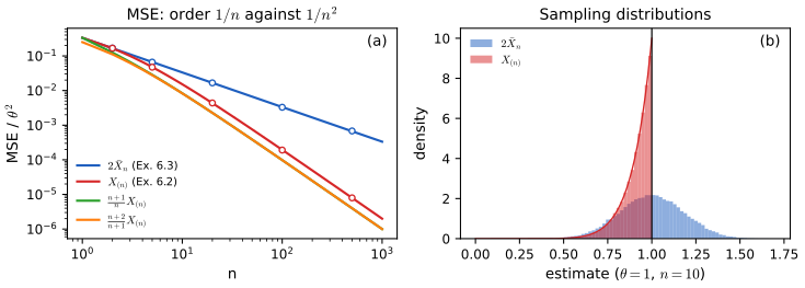
fig_6_s6. Download: PDF · SVGDemonstrations for this chapter
Each demonstration runs in the browser on simulated data and links back to these notes. The ▶ Demo boxes above open them already set to the case under discussion.
| Demonstration | What you can see | Sections and results |
|---|---|---|
| Coverage of intervals for a proportion | The exact coverage of the Wald, Wilson and Hoeffding intervals against \(p\) or against \(n\), their lowest coverage and expected width, and 100 simulated polls. Presets: 1 Wald against \(p\); 2 oscillation in \(n\); 3 small \(p\), no uniform guarantee; 4 Hoeffding; 5 Wilson. | 6.3.2, 6.5; Filling the gaps 6.12, 6.13, 6.15 |
| Bias, variance and MSE of shrinkage estimators | Exact bias², variance and MSE against the tuning value for \(c\overline X_n\), \((S+a)/(n+2a)\) and \(c\max_iX_i\); simulated sampling distributions; the risk function over all parameter values. Presets: 1 shrinking a Normal mean; 2 far from the target; 3 constant risk; 4 pseudo-counts near the edge; 5 the uniform endpoint. | 6.3.1; Theorem 6.9, Filling the gap 6.4; Exercises 6.2, 6.3 |
| Consistency as \(n\) grows | Sample paths of five estimators up to \(n=10\,000\), the exact probability of an error larger than \(\epsilon\), the fraction of simulated paths outside the band, and the Chebyshev and Hoeffding bounds. Presets: 1 a proportion; 2 a biased variance; 3 a maximum; 4 the Cauchy mean; 5 the Cauchy median. | Definition 6.7, Theorem 6.10; Filling the gaps 6.5, 6.6 |
Related demonstrations in the companion courses: the first-year confidence-interval demo (repeated intervals for a mean, with the normal and Student multipliers), the bias–variance demo of Bayesian and Probabilistic Machine Learning and the \(k\)-NN bias–variance demo of Statistical Learning: Theory and Methods. The Python code that produces every figure of this page is code/ch06_models_inference_learning.py (see the code index).
References
- Wasserman, L. (2004). All of Statistics: A Concise Course in Statistical Inference. Springer, New York. Chapter 6, pp. 87–96, and the Preface, p. xi. www.stat.cmu.edu/~larry/all-of-statistics.
- Agresti, A. and Coull, B. A. (1998). Approximate is better than "exact" for interval estimation of binomial proportions. The American Statistician, 52(2), 119–126.
- Berger, J. O. and Wolpert, R. L. (1984). The Likelihood Principle. Institute of Mathematical Statistics, Hayward, California.
- Bickel, P. J. and Doksum, K. A. (2000). Mathematical Statistics: Basic Ideas and Selected Topics, Vol. I, 2nd edition. Prentice Hall, Upper Saddle River.
- Brouwer, L. E. J. (1912). Beweis der Invarianz des n-dimensionalen Gebiets. Mathematische Annalen, 71, 305–313.
- Brown, L. D., Cai, T. T. and DasGupta, A. (2001). Interval estimation for a binomial proportion. Statistical Science, 16(2), 101–133.
- Casella, G. and Berger, R. L. (2002). Statistical Inference, 2nd edition. Duxbury, Pacific Grove.
- Cox, D. R. and Hinkley, D. V. (2000). Theoretical Statistics. Chapman and Hall/CRC, Boca Raton.
- DeGroot, M. H. and Schervish, M. J. (2002). Probability and Statistics, 3rd edition. Addison-Wesley, Boston.
- Hodges, J. L. and Lehmann, E. L. (1950). Some problems in minimax point estimation. The Annals of Mathematical Statistics, 21(2), 182–197.
- Hoeffding, W. (1963). Probability inequalities for sums of bounded random variables. Journal of the American Statistical Association, 58(301), 13–30.
- Larsen, R. J. and Marx, M. L. (1986). An Introduction to Mathematical Statistics and Its Applications, 2nd edition. Prentice Hall, Englewood Cliffs.
- Le Cam, L. (1973). Convergence of estimates under dimensionality restrictions. The Annals of Statistics, 1(1), 38–53.
- Lehmann, E. L. (1986). Testing Statistical Hypotheses, 2nd edition. Wiley, New York.
- Lehmann, E. L. and Casella, G. (1998). Theory of Point Estimation, 2nd edition. Springer, New York.
- Rice, J. A. (1995). Mathematical Statistics and Data Analysis, 2nd edition. Duxbury, Belmont.
- Tsybakov, A. B. (2009). Introduction to Nonparametric Estimation. Springer, New York.
- van der Vaart, A. W. (1998). Asymptotic Statistics. Cambridge University Press, Cambridge.
- Wilson, E. B. (1927). Probable inference, the law of succession, and statistical inference. Journal of the American Statistical Association, 22(158), 209–212.
The numerical statements in the text (the bump pair and its total variation and Sobolev size, the shrinkage and pseudo-count formulas and their minimisers, the exact tail probabilities of the five estimators, the Cauchy facts, the coverage of the posterior interval and its prior average, Example 6.14, the polling margins, the exact coverage and width of the three intervals for a proportion, the Poisson limit at \(p=\lambda/n\), the sizes of the fair-coin test, and the solutions of the exercises) were confirmed numerically.