Simulation Methods
Almost every quantity in Bayesian inference is an integral: a posterior mean, a posterior probability, a marginal density, a normalising constant. In one or two dimensions they can be computed on a grid; in ten they cannot. This chapter replaces integrals by averages of random draws. Basic Monte Carlo averages draws from the distribution itself, and its error falls like \(1/\sqrt N\) in any dimension. Importance sampling averages reweighted draws from a convenient proposal, and works only if the proposal's tails are heavy enough. Markov chain Monte Carlo builds a chain whose long-run distribution is the target, so that it can sample distributions known only up to a constant. The book states the key facts briefly; these notes prove them (the central limit theorem for the estimate, the optimal proposal, detailed balance with the rejection step included, the ergodic theorem and the autocorrelation time, why Gibbs sampling is Metropolis-Hastings that never rejects), quantify what the book shows in pictures, and reproduce every example, finding along the way that two of the book's numbers cannot come from its stated data.
Ch. 1 Probability Ch. 2 Random variables Ch. 3 Expectation Ch. 4 Inequalities Ch. 5 Convergence Ch. 6 Models and inference Ch. 7 Estimating the CDF Ch. 8 Bootstrap Ch. 9 Parametric inference Ch. 10 Hypothesis testing Ch. 11 Bayesian inference Ch. 12 Decision theory Ch. 13 Regression Ch. 14 Multivariate models Ch. 15 Independence Ch. 16 Causal inference Ch. 17 Directed graphs Ch. 18 Undirected graphs Ch. 19 Log-linear models Ch. 20 Curve estimation Ch. 21 Orthogonal functions Ch. 22 Classification Ch. 23 Stochastic processes Ch. 24 Simulation
How to read these notes
They follow the book. Sections carry the book's numbers (24.1 to 24.7), equations keep their numbers \((24.1)\) to \((24.9)\), and numbered items keep the book's numbers (Examples 24.1 to 24.11, Theorem 24.5, Remarks 24.8 and 24.9). Results the book uses without a number, and new results needed to fill its gaps, are lettered (Theorem 24.A, Definition 24.A, ...); the book's three unnumbered algorithm boxes are Algorithms 24.A to 24.C. Section 24.5 is split into three subsections for navigation. The chapter has no appendix.
Filling the gaps. Wherever the book says "it can be shown", quotes a result without proof, or leaves an argument implicit, an orange Filling the gap box gives the full argument. Proofs and derivations start hidden: open one with its bar, or use the button below.
Figures and demonstrations. All four figures of the chapter are simulations and all four are reproduced; seven supplementary figures (24.S1 to 24.S7) illustrate the gaps and the exercises. All are produced by the Python code. The ▶ Demo boxes open an interactive demonstration already set to the case being discussed.
Main reference
L. Wasserman, All of Statistics: A Concise Course in Statistical Inference, Springer (2004), Chapter 24, pages 403–422 (book website: www.stat.cmu.edu/~larry/all-of-statistics). Section, equation, example and exercise numbers below refer to this book. Further reading is listed in the references.
The explanations, derivations, figures and code are my own; equations are cited by their numbers in the book.
Companion courses
Sampling methods are covered from the machine-learning side in three companion courses on this site. The overlapping material is:
- Bayesian and Probabilistic Machine Learning, Chapter 11 (sampling methods): the Monte Carlo estimator (Result 11.1), rejection sampling (Result 11.7), importance sampling and its self-normalised form (Results 11.10, 11.11, Filling the gap 11.6, Result 11.12), Markov chains and detailed balance (Results 11.16, 11.17), Metropolis-Hastings (Result 11.19), Gibbs sampling (Result 11.20), slice sampling and Hamiltonian Monte Carlo. Its demos: sampling basics, MCMC, slice sampling and HMC.
- Foundations of Deep Learning, Chapter 14 (sampling): Monte Carlo error and dimension (Result 14.1, Filling the gap 14.1), importance sampling (Result 14.6), when a chain converges (Filling the gap 14.4), Metropolis-Hastings and Gibbs (Results 14.9, 14.10), and Langevin sampling. Its demo: Langevin sampling.
- Statistical Learning: Theory and Methods, Section 8.6: the Gibbs sampler (Algorithm 8.3) and why the target is stationary (Result 8.10).
Those courses use sampling as a tool for models; this chapter asks how accurate a simulation estimate is and how to tell. Where a proof there is identical, these notes give a complete but shorter argument and link to the longer one. New here: the central limit theorem and interval for the Monte Carlo estimate (Theorem 24.A), the exact variance of importance sampling with Normal proposals and the threshold \(s^2>1/2\) (Filling the gap 24.6), the optimal proposal for a sign-changing \(h\) (24.7), detailed balance with the rejection atom (24.10), the stationary acceptance rate \((2/\pi)\arctan(2/b)\) (24.13), the geometric convergence of the independence sampler (24.15), the exact posterior of Example 24.11 used to check the Gibbs sampler (24.17), and the Gelman-Rubin diagnostic (24.19).
The chapter at a glance
- 24.1 Posterior means, marginals and normalising constants are integrals, often high-dimensional (Filling the gap 24.1).
- 24.2 Basic Monte Carlo: \(\hI=N^{-1}\sum w(X_i)\) with \(X_i\sim f\) is unbiased, consistent and asymptotically Normal with standard error \(\sigma/\sqrt N\), whatever the dimension (Theorem 24.A). Posterior simulation turns Bayesian questions into averages (Examples 24.3 and 24.4).
- 24.3 Importance sampling: \(\hI=N^{-1}\sum h(X_i)f(X_i)/g(X_i)\) with \(X_i\sim g\) is unbiased, with variance \((24.6)\) that is infinite when \(g\) has lighter tails than \(hf\) (Theorem 24.B, Filling the gap 24.6); the optimal \(g\) is proportional to \(|h|f\) (Theorem 24.5). Self-normalised weights handle unnormalised posteriors (Filling the gap 24.8); the effective sample size summarises the weights (Definition 24.A).
- 24.4 Metropolis-Hastings (Algorithm 24.A) satisfies detailed balance, so \(f\) is stationary (Theorem 24.C); an ergodic theorem and a central limit theorem make chain averages consistent, with error \(\sigma\sqrt{\tau/N}\) (Filling the gaps 24.11, 24.12).
- 24.5 Random-walk and independence proposals and their tuning (24.13–24.15); Gibbs sampling, which is Metropolis-Hastings with acceptance probability 1 (Result 24.D); the hierarchical model of Example 24.11; Metropolis within Gibbs; convergence diagnostics (24.19).
Notation. \(f\) is a target density (often a posterior), \(h\) a function whose mean \(I=\E_f h(X)=\int hf\) is wanted, \(g\) a proposal density we can sample, and \(N\) the number of draws. \(\hI\) is an estimate of \(I\), \(\se\) its standard deviation and \(\hse\) an estimate of that. \(\phi\) and \(\Phi\) are the standard Normal density and cdf. For a Markov chain, \(q(y\given x)\) is the proposal density, \(r(x,y)\) the acceptance probability and \(P(x,\cdot)\) the transition kernel.
Prerequisites. The laws of large numbers and the central limit theorem (Theorems 5.6, 5.8, 5.10, 5.18), Jensen's inequality (Theorem 4.9), the delta method (Theorem 5.13), posterior simulation (Section 11.4) and Markov chains (Section 23.2; the ergodic theorem is Theorem 23.25). See the course home.
24.1 Bayesian Inference Revisited
pp. 403–404 With prior \(f(\th)\) and likelihood \(\mathcal L(\th)\) the posterior is \(f(\th\given x^n)=\mathcal L(\th)f(\th)/c\), where \(c=\int\mathcal L(\th)f(\th)\,\d\th\). The posterior mean is a ratio of two integrals,
\[\bar\th=\int\th f(\th\given x^n)\,\d\th=\frac{\int\th\,\mathcal L(\th)f(\th)\,\d\th}{\int\mathcal L(\th)f(\th)\,\d\th},\]and when \(\th=(\th_1,\dots,\th_k)\) the marginal posterior of \(\th_1\) is a \((k-1)\)-dimensional integral, \(f(\th_1\given x^n)=\int\!\cdots\!\int f(\th_1,\dots,\th_k\given x^n)\,\d\th_2\cdots\d\th_k\). The rest of the chapter is about computing such integrals. (Chapter 11 of the notes covers the Bayesian method itself: Section 11.2.)
Filling the gap 24.1: why these integrals are hard, and what a sample buys p. 404
Grids do not scale. A grid with \(m\) points per coordinate has \(m^k\) points: with \(m=100\) and \(k=10\) that is \(10^{20}\) evaluations. Worse, a posterior concentrates on a region of width about \(1/\sqrt n\) per coordinate, so most grid points carry negligible mass.
A sample answers every question at once. If \(\th^{(1)},\dots,\th^{(N)}\) are draws from the posterior, then: the posterior mean of any \(g(\th)\) is estimated by the average of \(g(\th^{(i)})\); a posterior probability \(\P(\th\in A\given x^n)\) by the proportion of draws in \(A\); a posterior quantile by the sample quantile; and the marginal posterior of \(\th_1\) by simply keeping the first coordinate of each draw. The last point is the reason simulation is so convenient: integrating out \(\th_2,\dots,\th_k\) costs nothing, because the first coordinates of draws from the joint are draws from the marginal (Filling the gap 11.14).
Why projection gives the marginal
If \(\th=(\th_1,\th_{-1})\) has density \(f(\th_1,\th_{-1})\), then for any set \(A\), \(\P(\th_1\in A)=\P(\th\in A\times\R^{k-1})\)
24.2 Basic Monte Carlo Integration
pp. 404–408 To compute \(I=\int_a^bh(x)\,\d x\), write it as an expectation under the uniform density \(f(x)=1/(b-a)\):
\[I=\int_a^bh(x)\,\d x=\int_a^bw(x)f(x)\,\d x=\E_f\,w(X),\qquad w(x)=h(x)(b-a).\tag{24.1}\]With \(X_1,\dots,X_N\sim\Unif(a,b)\) independent, the law of large numbers gives
\[\hI\equiv\frac1N\sum_{i=1}^Nw(X_i)\ \xrightarrow{\ \P\ }\ \E\,w(X)=I.\tag{24.2}\]The standard error is estimated by \(\hse=s/\sqrt N\), where \(s^2=\sum_i(Y_i-\hI)^2/(N-1)\) and \(Y_i=w(X_i)\), and \(\hI\pm z_{\alpha/2}\hse\) is an approximate \(1-\alpha\) confidence interval for \(I\). More generally, for a density \(f\) that we can sample,
\[I=\int h(x)f(x)\,\d x\tag{24.3}\]is estimated by \(\hI=N^{-1}\sum_ih(X_i)\) with \(X_i\sim f\). (The book's statement uses \(\hI\equiv\) for the estimate; the \(\equiv\) there is a definition.)
Theorem 24.A (the basic Monte Carlo estimate) pp. 404–405
Let \(X_1,\dots,X_N\) be iid with density \(f\), \(Y_i=h(X_i)\), \(I=\E\,Y_1\) and \(\hI=\bar Y_N\). Then
- if \(\E|Y_1|<\infty\): \(\E\,\hI=I\), and \(\hI\to I\) in probability and almost surely;
- if \(\sigma^2=\V(Y_1)<\infty\): \(\V(\hI)=\sigma^2/N\), so \(\se(\hI)=\sigma/\sqrt N\);
- if moreover \(\sigma^2>0\): \(\sqrt N(\hI-I)/\sigma\rightsquigarrow\N(0,1)\), and also \((\hI-I)/\hse\rightsquigarrow\N(0,1)\), so \(\P(I\in\hI\pm z_{\alpha/2}\hse)\to1-\alpha\).
Filling the gap 24.2: proof of Theorem 24.A, and why the rate does not depend on the dimension
Proof
(1) By linearity \(\E\,\hI=N^{-1}\sum\E\,Y_i=I\). Consistency in probability is the weak law (Theorem 5.6; with only a first moment, Filling the gap 5.5), almost sure consistency the strong law (Theorem 5.18). (2) By independence \(\V(\hI)=N^{-2}\sum\V(Y_i)=\sigma^2/N\). (3) The first statement is the central limit theorem (Theorem 5.8). For the second, \(s^2\to\sigma^2\) in probability (write \(s^2=\frac N{N-1}(\overline{Y^2}-\bar Y^2)\) and apply the weak law to \(Y\) and \(Y^2\)), so \(\sigma/s\to1\) and, by Slutsky's theorem, \((\hI-I)/\hse=\frac{\sigma}{s}\cdot\sqrt N(\hI-I)/\sigma\rightsquigarrow\N(0,1)\) (Theorem 5.10). Hence \(\P(|\hI-I|\le z_{\alpha/2}\hse)\)
The dimension. Nothing in the theorem refers to the dimension of \(X\): the error is \(\sigma/\sqrt N\), and \(\sigma^2=\V_f\,h(X)\) depends only on how variable \(h\) is under \(f\). Compare a product rule on a grid of \(N=m^k\) points in \(k\) dimensions: the trapezoid rule has error of order \(m^{-2}=N^{-2/k}\) for smooth integrands, Simpson's rule \(N^{-4/k}\). Monte Carlo's \(N^{-1/2}\) is worse than the trapezoid rule for \(k\le3\) and better for \(k\ge5\); it beats Simpson's rule from \(k\ge9\). In the posteriors of this chapter, \(k\) is 10 (Example 24.4) or 21 (Example 24.11). The dimension can still enter through \(\sigma^2\), which may grow with \(k\); the companion course discusses this (Filling the gap 14.1 of Foundations of Deep Learning).
Relative error. For a probability \(I=\P(A)\), \(h=\ind_A\) and \(\sigma^2=I(1-I)\), so the relative error \(\se/I=\sqrt{(1-I)/(NI)}\) blows up for rare events: about \(1/(NI)\) draws must hit \(A\) before the estimate means anything. That is the motivation for importance sampling (Example 24.6).
See also Result 11.1 of Bayesian and Probabilistic Machine Learning and Result 14.1 of Foundations of Deep Learning; and, for the Monte Carlo error of a bootstrap, Filling the gap 8.2.
Example 24.1 (\(\int_0^1x^3\,\d x\)). p. 405 Here \(I=1/4\), \(w(x)=x^3\) and \(\sigma^2=\E X^6-(\E X^3)^2=1/7-1/16=9/112\), so with \(N=10{,}000\) the exact standard error is \(\sqrt{9/112}/100=0.00283\). The book reports \(\hI=0.248\) with \(\hse=0.0028\); our run gives \(0.2502\) with \(\hse=0.00284\). Both are well within one standard error of \(1/4\).
Example 24.2 (a Normal cdf). p. 405 \(\Phi(x)=\E\,\ind\{Z\le x\}\) for \(Z\sim\N(0,1)\), so \(\hI\) is the proportion of Normal draws at most \(x\), with \(\sigma^2=\Phi(x)(1-\Phi(x))\). For \(x=2\), \(\Phi(2)=0.97725\) and the standard error is \(0.0015\) at \(N=10^4\) and \(0.00047\) at \(N=10^5\). The book's estimates \(0.9751\) and \(0.9771\) are 1.4 and 0.3 standard errors away; ours are \(0.9769\) and \(0.97706\).
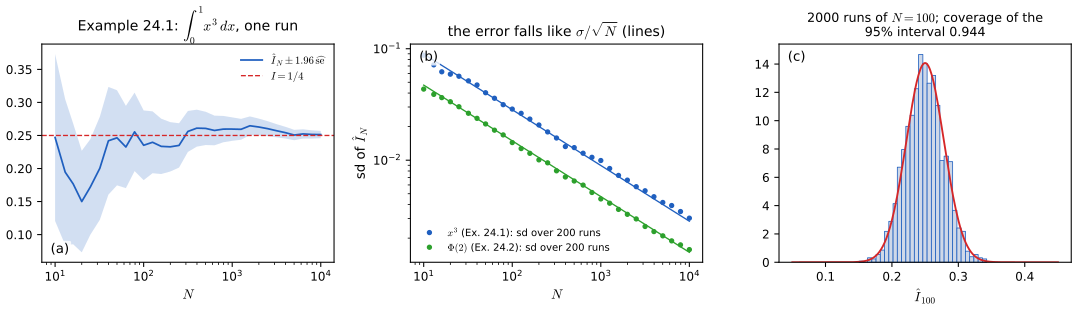
fig_24_s1. Download: PDF · SVGExample 24.3 (Bayesian inference for two binomials). pp. 406–407 Let \(X\sim\Bin(n,p_1)\) and \(Y\sim\Bin(m,p_2)\) be independent and \(\delta=p_2-p_1\). The MLE is \(\hat\delta=Y/m-X/n\), with delta-method standard error \(\hse=\sqrt{\hat p_1(1-\hat p_1)/n+\hat p_2(1-\hat p_2)/m}\). With the flat prior \(f(p_1,p_2)=1\) the posterior factorises,
\[f(p_1,p_2\given X,Y)\propto p_1^X(1-p_1)^{n-X}\,p_2^Y(1-p_2)^{m-Y},\]so \(p_1\) and \(p_2\) are independent a posteriori with \(p_1\given X\sim\Beta(X+1,n-X+1)\) and \(p_2\given Y\sim\Beta(Y+1,m-Y+1)\). Instead of computing the posterior mean \(\iint(p_2-p_1)f(p_1,p_2\given X,Y)\,\d p_1\d p_2\) and the posterior cdf of \(\delta\) as integrals over \(\{p_2-p_1\le c\}\), draw \(P_1^{(i)}\) and \(P_2^{(i)}\) from the two Beta posteriors and set \(\delta^{(i)}=P_2^{(i)}-P_1^{(i)}\): the average estimates the posterior mean, the 2.5% and 97.5% sample quantiles give a 95% posterior interval, and a histogram estimates the density. With \(n=m=10\), \(X=8\), \(Y=6\): the exact posterior mean is \(7/12-9/12=-1/6\), the exact 95% interval (by numerical convolution) is \((-0.527,0.192)\), and 1000 draws give mean \(-0.169\) and interval \((-0.53,0.18)\); the book's \((-0.52,0.20)\) agrees within the Monte Carlo error of a sample quantile from 1000 draws (about 0.02). The frequentist analysis gives \(\hat\delta=-0.2\), \(\hse=0.2\) and the interval \(\hat\delta\pm2\hse=(-0.6,0.2)\). The same example is Example 11.7 of the book (notes).
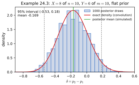
fig_24_1. Download: PDF · SVGFilling the gap 24.3: why the simulated interval and histogram are valid p. 406
The \(\delta^{(i)}\) are iid draws from the posterior of \(\delta\). Their empirical cdf converges uniformly to the posterior cdf (Glivenko-Cantelli), so the sample \(q\)-quantile converges to the posterior \(q\)-quantile whenever the posterior cdf is continuous and strictly increasing there, with standard deviation about \(\sqrt{q(1-q)/N}/f(\xi_q)\), where \(f(\xi_q)\) is the posterior density at the quantile (Filling the gap 7.11). Here \(f(\xi_{0.025})\approx0.3\), so with \(N=1000\) the interval end points are uncertain by about \(\pm0.02\): a second decimal is all one should report. A histogram with bin width \(h\) is a density estimate with bias of order \(h\) and variance of order \(1/(Nh)\) (the book's Chapter 20). The posterior mean is the average, with standard error \(\sigma_\delta/\sqrt N\) (Theorem 24.A), here \(0.18/\sqrt{1000}\approx0.006\).
Filling the gap 24.4: Beta draws from uniforms
To draw a \(\Beta(k,n-k+1)\) variable with integer parameters, it suffices to take the \(k\)-th smallest of \(n\) independent \(\Unif(0,1)\) variables. The Monte Carlo demo draws the Beta posteriors of Example 24.3 this way.
Proof
Let \(U_{(k)}\) be the \(k\)-th smallest. \(U_{(k)}\le t\) exactly when at least \(k\) of the \(n\) uniforms are at most \(t\), and the number of those is \(\Bin(n,t)\). So \(F(t)=\sum_{j=k}^n\binom nj t^j(1-t)^{n-j}\). Differentiating, the terms telescope:
\[F'(t)=\sum_{j=k}^n\Big[j\tbinom nj t^{j-1}(1-t)^{n-j}-(n-j)\tbinom nj t^j(1-t)^{n-j-1}\Big]=\frac{n!}{(k-1)!\,(n-k)!}\,t^{k-1}(1-t)^{n-k},\]because \((n-j)\binom nj=(j+1)\binom n{j+1}\), so the negative part of term \(j\) cancels the positive part of term \(j+1\), and only the positive part of \(j=k\) survives. The right side is the \(\Beta(k,n-k+1)\) density. ∎
Example 24.4 (Bayesian inference for dose response). pp. 407–408 Rats receive one of ten doses \(x_1<\dots<x_{10}\) (here \(x_i=i\)), \(n=15\) at each, and \(Y_i\sim\Bin(n,p_i)\) are the numbers that die (the book says "survive", but its analysis and its data treat \(Y_i\) as deaths; see the notes on the book). Biology says \(p_1\le p_2\le\dots\le p_{10}\). The target is the LD50, the first dose at which death is at least as likely as not: \(\delta=x_j\) with \(j=\min\{i:p_i\ge1/2\}\). Its posterior mean and cdf are 10-dimensional integrals over the ordered region \(A=\{p_1\le\dots\le p_{10}\}\). With a flat prior truncated to \(A\), simulation is easy:
- draw \(P_i\sim\Beta(Y_i+1,n-Y_i+1)\) independently, \(i=1,\dots,10\);
- keep the draw if \(P_1\le\dots\le P_{10}\), otherwise discard it and return to step 1;
- set \(\delta=x_j\) with \(j=\min\{i:P_i>1/2\}\).
Repeating gives \(\delta^{(1)},\dots,\delta^{(N)}\); their average estimates \(\E(\delta\given Y)\) and their frequencies the posterior mass function \(\P(\delta=x_j\given Y)\). For the book's data (deaths \(0,0,2,2,8,10,12,14,15,14\)) about 0.73% of the proposals are ordered, and 5000 kept draws give posterior probabilities 0.47 for \(\delta=5\), 0.48 for \(\delta=6\) and 0.05 for \(\delta=7\): a posterior mean of 5.58 and a 95% interval of \((5,7)\). The book reports 4.04 and \((3,5)\), which these data cannot produce (notes on the book).
Filling the gap 24.5: discarding unordered draws gives exactly the truncated posterior p. 408
With prior \(\pi(p)\propto\ind_A(p)\) the posterior is \(f(p\given Y)\propto\ind_A(p)\prod_i p_i^{Y_i}(1-p_i)^{n-Y_i}\), that is, the product of the ten Beta posteriors conditioned on the event \(A\). Steps 1 and 2 are rejection sampling for that conditional distribution: each round draws \(P\) from the unconstrained product \(f_0\); the rounds are independent; the kept draw is the first \(P\) in \(A\). For any set \(B\),
\[\P(\text{kept draw}\in B)=\sum_{t\ge1}(1-f_0(A))^{t-1}f_0(A\cap B)=\frac{f_0(A\cap B)}{f_0(A)},\]which is the probability of \(B\) under \(f_0\) restricted to \(A\) and renormalised, i.e. under the truncated posterior. The number of rounds per kept draw is geometric with mean \(1/f_0(A)\), here about 137. (This is the accept-reject method of Exercise 3 with \(f\le Mg\), \(g=f_0\) and \(M=1/f_0(A)\): a draw is accepted with probability \(\ind_A\).) The cost grows quickly with the number of constraints; for longer chains of doses a Gibbs sampler with truncated Beta conditionals is the standard alternative.
See also rejection sampling in Result 11.7 of Bayesian and Probabilistic Machine Learning.
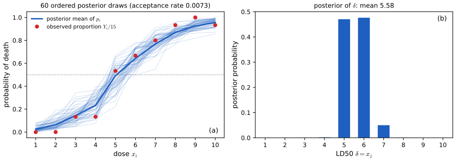
fig_24_s2. Download: PDF · SVG24.3 Importance Sampling
pp. 408–411 Basic Monte Carlo needs draws from \(f\). When we cannot draw from \(f\), but can evaluate it, we draw from a density \(g\) that we can sample and reweight:
\[I=\int h(x)f(x)\,\d x=\int\frac{h(x)f(x)}{g(x)}\,g(x)\,\d x=\E_g(Y),\qquad Y=\frac{h(X)f(X)}{g(X)},\ X\sim g,\tag{24.4}\] \[\hI=\frac1N\sum_{i=1}^N\frac{h(X_i)f(X_i)}{g(X_i)},\qquad X_1,\dots,X_N\sim g.\tag{24.5}\]The terms have second moment
\[\E_g\big(w^2(X)\big)=\int\Big(\frac{h(x)f(x)}{g(x)}\Big)^2g(x)\,\d x=\int\frac{h^2(x)f^2(x)}{g(x)}\,\d x,\qquad w=\frac{hf}{g},\tag{24.6}\]which can be infinite.
Theorem 24.B (importance sampling) p. 409
Suppose \(g(x)>0\) wherever \(h(x)f(x)\ne0\) and \(\int|h|f<\infty\). Then \(\E_g\,\hI=I\) and \(\hI\to I\) almost surely. Its variance is \(\V(\hI)=\big(\int h^2f^2/g-I^2\big)/N\); if this is finite and positive, \(\sqrt N(\hI-I)\rightsquigarrow\N\big(0,\int h^2f^2/g-I^2\big)\). If \(\int h^2f^2/g=\infty\), \(\hI\) is still consistent but has infinite variance, and its error is not of order \(1/\sqrt N\).
Proof
The terms \(Y_i=w(X_i)\) are iid with \(\E_g|Y_i|=\int|h|f<\infty\) and \(\E_gY_i=\int_{\{g>0\}}hf=I\), using the support condition (if \(g=0\) on a set where \(hf\ne0\), that part of \(I\) is never seen). Everything then follows from Theorem 24.A applied to the \(Y_i\), with \(\V(Y_1)=\E_gY_1^2-I^2\) and \((24.6)\). ∎
See also Result 11.10 of Bayesian and Probabilistic Machine Learning and Result 14.6 of Foundations of Deep Learning.
Filling the gap 24.6: light-tailed proposals give infinite variance, exactly p. 409
The book says that if \(g\) has thinner tails than \(f\) the integral \((24.6)\) "might be" infinite. For Normal densities the condition is explicit. Let \(f=\N(0,1)\) and \(g=\N(\mu,s^2)\). Then
\[\frac{f(x)^2}{g(x)}=\frac{s}{\sqrt{2\pi}}\exp\Big(-x^2+\frac{(x-\mu)^2}{2s^2}\Big),\]and the coefficient of \(x^2\) in the exponent is \(-1+1/(2s^2)\). So \(\int_c^\infty f^2/g<\infty\) if and only if \(s^2>1/2\) (for \(s^2=1/2\) it depends on the sign of \(\mu\)). With \(k=2s^2-1>0\), completing the square gives the closed form
\[\int_c^\infty\frac{f(x)^2}{g(x)}\,\d x=\frac{s^2}{\sqrt k}\,e^{\mu^2/k}\;\P(W>c),\qquad W\sim\N\big(-\mu/k,\ s^2/k\big).\]A proposal centred in the right place but too narrow (for Example 24.6, \(g=\N(4,0.6^2)\)) therefore has infinite variance; the sample variance of the terms keeps jumping as rare large weights arrive, and the estimated standard error is meaningless. If \(f\) is a \(t\) or Cauchy density, every Normal proposal gives \(f^2/g\sim|x|^{-2(\nu+1)}e^{x^2/(2s^2)}\to\infty\): infinite variance whatever \(s\). The rule "\(g\) must have heavier tails than \(hf\)" guarantees that \(hf/g\) stays bounded in the tails, which with \(\int|h|f<\infty\) and bounded \(h\) gives a finite second moment.
The completed square
The exponent is \(-ax^2-(\mu/s^2)x+\mu^2/(2s^2)\) with \(a=k/(2s^2)\). Writing it as \(-a(x+\mu/k)^2+\mu^2/k\) (check: \(a(\mu/k)^2=\mu^2/(2s^2k)\) and \(\mu^2/(2s^2k)+\mu^2/(2s^2)=\mu^2/k\)), the integral of \(\exp(-a(x+\mu/k)^2)\) over \((c,\infty)\) is \(\sqrt{\pi/a}\,\P(W>c)\) with \(\V(W)=1/(2a)=s^2/k\). Multiplying by \(s/\sqrt{2\pi}\) and \(e^{\mu^2/k}\) gives \(s\sqrt{s^2/k}\,e^{\mu^2/k}\P(W>c)\). ∎
See also Filling the gap 11.6 of Bayesian and Probabilistic Machine Learning.
Theorem 24.5 (the optimal proposal) pp. 409–410
Among densities \(g\) with \(g>0\) where \(hf\ne0\), the variance of \(\hI\) is minimised by
\[g^*(x)=\frac{|h(x)|f(x)}{\int|h(s)|f(s)\,\d s},\]and the minimum variance is \(\big[(\int|h|f)^2-I^2\big]/N\), which is 0 when \(h\ge0\).
Filling the gap 24.7: the proof, completed pp. 409–410
Proof
Write \(W=w(X)=h(X)f(X)/g(X)\) with \(X\sim g\). Its variance is \(\E_g(W^2)-(\E_gW)^2\) (the book prints \((\E(W^2))^2\) for the second term; listed in the author's errata), and \(\E_gW=I\) does not depend on \(g\). So it suffices to minimise \(\E_g(W^2)\). By Jensen's inequality (Theorem 4.9), or simply \(\V_g(|W|)\ge0\),
\[\E_g(W^2)\ \ge\ \big(\E_g|W|\big)^2=\Big(\int\frac{|h|f}{g}\,g\Big)^2=\Big(\int|h|f\Big)^2,\]a bound that does not depend on \(g\). Under \(g^*\), \(|W|=|h|f/g^*=\int|h|f\) is constant wherever \(g^*>0\), so \(\E_{g^*}(W^2)=(\int|h|f)^2\) attains the bound. Equality in \(\V_g(|W|)\ge0\) holds only when \(|W|\) is \(g\)-almost surely constant, i.e. \(g\propto|h|f\): the minimiser is unique (up to null sets). If \(h\ge0\), \(\int|h|f=I\) and the minimum variance is \(I^2-I^2=0\): every term equals \(I\). If \(h\) changes sign, the minimum is \((\int|h|f)^2-I^2>0\); zero variance can then be had by estimating \(\int h^+f\) and \(\int h^-f\) separately, each with its own optimal proposal. ∎
The theorem is a guide rather than a method: drawing from \(g^*\) requires its normalising constant, which for \(h\ge0\) is \(I\) itself. In practice one looks for a \(g\) of roughly the shape of \(|h|f\) with heavier tails. Both the zero-variance case and its failure for a sign-changing \(h\) are confirmed numerically.
Example 24.6 (tail probability). p. 410 Estimate \(I=\P(Z>3)=0.00135\), \(Z\sim\N(0,1)\), with \(N=100\). Plain Monte Carlo has standard deviation \(\sqrt{I(1-I)/100}=0.00367\), almost three times \(I\); 87% of runs see no draw beyond 3 at all. Drawing instead from \(g=\N(4,1)\), which puts its mass where \(h=1\), gives terms \(\ind\{X>3\}\phi(X)/\phi(X-4)=\ind\{X>3\}e^{8-4X}\). By Filling the gap 24.6 (\(s=1\), \(k=1\)) their second moment is \(e^{16}\P(Z>7)\), so the standard deviation of \(\hI\) is 0.00031: twelve times smaller. Over 10,000 repetitions we find 0.00367 and 0.00030. The book's "\(\V(\hI)=.0039\)" and ".0002" are standard deviations, not variances (notes on the book).
Example 24.7 (measurement model with outliers). pp. 410–411 Measurements \(X_i=\th+\epsilon_i\) with \(t_\nu\) errors, whose density is
\[t(x)=\frac{\Gamma\big(\frac{\nu+1}2\big)}{\Gamma\big(\frac\nu2\big)}\,\frac1{\sqrt{\nu\pi}}\Big(1+\frac{x^2}\nu\Big)^{-(\nu+1)/2}\](the book omits the square root; notes on the book), are robust to outliers because the tails are heavy. With \(\nu=3\), a flat prior and likelihood \(\mathcal L(\th)=\prod_it(X_i-\th)\), the posterior mean is \(\int\th\mathcal L/\int\mathcal L\), a ratio of integrals that importance sampling estimates by a ratio of averages:
\[\bar\th\approx\frac{\frac1N\sum_j\th_j\mathcal L(\th_j)/g(\th_j)}{\frac1N\sum_j\mathcal L(\th_j)/g(\th_j)},\qquad \th_1,\dots,\th_N\sim g.\]The book does not print its two observations, but for \(n=2\) the posterior is symmetric about \((X_1+X_2)/2\) (Filling the gap 24.8), so its posterior mean \(-0.54\) fixes their average. We take \(X=(-3.04,1.96)\). With \(N=10{,}000\) draws from the standard Normal the estimate is \(-0.63\) (effective sample size 470), from the standard Cauchy \(-0.56\) (effective sample size 5240): the same pattern as the book's \(-0.74\) and \(-0.53\). The Normal proposal has infinite variance here, the Cauchy a finite one.
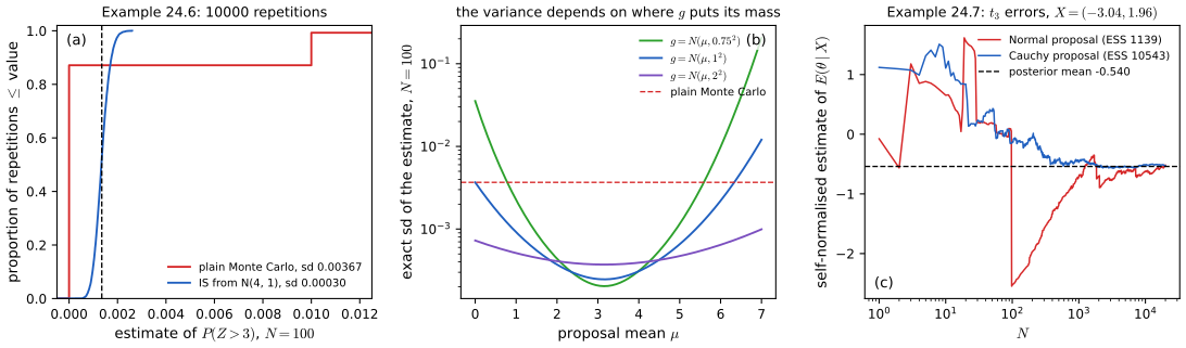
fig_24_s3. Download: PDF · SVGFilling the gap 24.8: self-normalised importance sampling p. 411
Let \(\pi=\mathcal L f/c\) be a posterior known only up to \(c\), \(w=\mathcal L f/g\) the unnormalised weight, and \(\hI=\sum_jw(\th_j)h(\th_j)/\sum_jw(\th_j)\) with \(\th_j\sim g\).
- Consistency. By the strong law, the numerator average tends to \(\E_g(wh)=\int h\mathcal Lf=cI\) and the denominator average to \(\E_gw=c\), so \(\hI\to I\) almost surely. The constant \(c\) cancels: that is why the method works for unnormalised posteriors.
- Asymptotic variance. By the bivariate central limit theorem and the delta method (Theorem 5.15) applied to \((a,b)\mapsto a/b\),
provided the integral is finite. The gradient of \(a/b\) at \((cI,c)\) is \((1/c,-I/c)\), so the asymptotic variance is \(\V_g\big(wh/c-Iw/c\big)=\E_g[w^2(h-I)^2]/c^2\). The estimator is biased, with bias of order \(1/N\) (a second-order delta-method term), negligible next to its standard deviation.
The posterior for \(n=2\) is symmetric. Let \(m=(X_1+X_2)/2\) and \(d=(X_2-X_1)/2\). Then \(\mathcal L(m+u)=t(d+u)\,t(d-u)\) (using \(t(-x)=t(x)\)), which is even in \(u\). With a flat prior the posterior is symmetric about \(m\), and its mean, which exists because the posterior decays like \(|\th|^{-8}\), equals \(m\). In Example 24.7 the variance integral is infinite for a Normal \(g\) (the posterior tails are polynomial) and finite for a Cauchy \(g\), where it equals 9.10, so the Cauchy-based estimate has standard deviation \(\sqrt{9.10/N}\); 400 runs of \(N=2000\) confirm it.
See also Result 11.11 of Bayesian and Probabilistic Machine Learning.
Definition 24.A (effective sample size of importance weights)
For weights \(w_1,\dots,w_N\ge0\), \(\ESS=\big(\sum_iw_i\big)^2\big/\sum_iw_i^2\). It lies between 1 (one weight carries everything) and \(N\) (equal weights).
Filling the gap 24.9: where the effective sample size comes from
Kong (1992) showed that, to first order, the variance of the self-normalised estimate is that of an iid average of \(N/(1+\mathrm{cv}^2)\) draws from \(\pi\), where \(\mathrm{cv}^2=\V_g(w)/(\E_gw)^2\) is the squared coefficient of variation of the normalised weights. Replacing \(\mathrm{cv}^2\) by its sample version \(\widehat{\mathrm{cv}}^2=N\sum w_i^2/(\sum w_i)^2-1\) (divisor \(N\)) gives exactly \(N/(1+\widehat{\mathrm{cv}}^2)=(\sum w_i)^2/\sum w_i^2\). It is a diagnostic, not a guarantee: it measures how unequal the weights are among the draws obtained, and a proposal that misses part of the target entirely can show a large ESS. With infinite-variance weights it is erratic from run to run, as the demonstration shows.
Derivation of Kong's approximation
Normalise the weights so that \(\E_gw=1\). From Filling the gap 24.8, \(N\V(\hI)\approx\E_g[w^2(h-I)^2]\). If \(w\) and \((h-I)^2\) are roughly uncorrelated under \(g\) (the approximation), this is \(\E_g(w^2)\,\E_g[(h-I)^2]\). Now \(\E_g(w^2)=1+\mathrm{cv}^2\), and \(\E_g[(h-I)^2]\) is close to \(\E_\pi[(h-I)^2]=\V_\pi(h)\) when \(g\) is close to \(\pi\). So \(\V(\hI)\approx\V_\pi(h)(1+\mathrm{cv}^2)/N\), the variance of a mean of \(N/(1+\mathrm{cv}^2)\) iid draws from \(\pi\). ∎
See also Result 11.12 of Bayesian and Probabilistic Machine Learning.
24.4 MCMC Part I: The Metropolis–Hastings Algorithm
pp. 411–414 Markov chain Monte Carlo builds a Markov chain \(X_1,X_2,\dots\) whose stationary distribution is \(f\), and estimates \(I=\E_fh(X)\) by \(N^{-1}\sum_{i=1}^Nh(X_i)\). This works because Markov chains have a law of large numbers (Theorem 23.25, for countable state spaces; Filling the gap 24.11 for general ones). The proposal \(q(y\given x)\) is any conditional density we can sample.
Algorithm 24.A (Metropolis–Hastings) pp. 411–412
Choose \(X_0\) arbitrarily. Given \(X_0,\dots,X_i\):
- generate a proposal \(Y\sim q(y\given X_i)\);
- compute \(r=r(X_i,Y)\), where
- set \(X_{i+1}=Y\) with probability \(r\), and \(X_{i+1}=X_i\) with probability \(1-r\).
Only ratios of \(f\) appear, so \(f\) need only be known up to a constant: a posterior \(\mathcal L(\th)f(\th)\) without its normalising constant is enough.
Remark 24.8 p. 412
Step 3 is carried out by drawing \(U\sim\Unif(0,1)\) and accepting when \(U<r\).
Remark 24.9 p. 412
A common proposal is \(q(y\given x)=\N(x,b^2)\). It is symmetric, \(q(y\given x)=q(x\given y)\), so \(r=\min\{f(Y)/f(X_i),1\}\): the original Metropolis algorithm.
Example 24.10 (a Cauchy target). pp. 412–413 For \(f(x)=\pi^{-1}(1+x^2)^{-1}\) and \(q=\N(x,b^2)\), \(r(x,y)=\min\{(1+x^2)/(1+y^2),1\}\). Figure 24.2 runs three chains of length 1000 from \(X_0=0\). With \(b=0.1\) almost every proposal is accepted (98%) but the chain moves slowly and in 1000 steps never leaves \((-1.3,1.6)\); with \(b=10\) only 28% are accepted and the chain often stays put; \(b=1\) accepts 75%. The book judges the middle chain best. Measured more carefully (Filling the gap 24.13), the heavy Cauchy tails make \(b=10\) the better of the two: over 100 chains its average Kolmogorov-Smirnov distance to the target is 0.094 against 0.125, and its effective sample size 126 against 38.
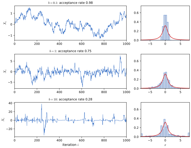
fig_24_2. Download: PDF · SVGWhy it works. pp. 413–414 For a continuous state space write \(p(x,y)\) for the transition density from \(x\) to \(y\). A density \(f\) is stationary if \(f(x)=\int f(y)p(y,x)\,\d y\), and satisfies detailed balance if
\[f(x)p(x,y)=f(y)p(y,x).\tag{24.7}\]Detailed balance implies stationarity (the continuous version of Theorem 23.26): \(\int f(y)p(y,x)\,\d y=\int f(x)p(x,y)\,\d y\)
and \((24.8)\) and \((24.9)\) agree.
Theorem 24.C (Metropolis–Hastings leaves \(f\) invariant)
Let \(f\) be a density and \(q(\cdot\given x)\) a proposal density for every \(x\) with \(f(x)>0\). The Metropolis-Hastings transition kernel
\[P(x,A)=\int_Aq(y\given x)r(x,y)\,\d y+\rho(x)\,\ind_A(x),\qquad\rho(x)=1-\int q(y\given x)r(x,y)\,\d y,\]satisfies detailed balance in the form \(f(x)q(y\given x)r(x,y)=f(y)q(x\given y)r(y,x)\) for all \(x,y\), and \(\int f(x)P(x,A)\,\d x=\int_Af\) for every set \(A\): if \(X_i\sim f\) then \(X_{i+1}\sim f\).
Filling the gap 24.10: the rejection step, and a one-line proof of detailed balance pp. 413–414
The book's argument treats \(p(x,y)\) as a density, but the Metropolis-Hastings kernel is not absolutely continuous: with probability \(\rho(x)\) the chain stays exactly at \(x\), an atom. The argument still works because the atom is symmetric by itself; here is the complete version, which also needs no case distinction.
Proof of Theorem 24.C
Detailed balance of the moving part. For \(f(x)q(y\given x)>0\),
\[f(x)q(y\given x)r(x,y)=f(x)q(y\given x)\min\Big\{\frac{f(y)q(x\given y)}{f(x)q(y\given x)},1\Big\}=\min\{f(y)q(x\given y),\,f(x)q(y\given x)\},\]which is symmetric in \(x\) and \(y\); if \(f(x)q(y\given x)=0\) both sides are 0 under the convention \(r=0\) there (a proposal that cannot be made is never accepted). Ties need no special treatment.
Invariance. For any set \(A\), split \(\int f(x)P(x,A)\,\d x\) into its two parts. Using the symmetry just shown and then Fubini,
\[\int f(x)\int_Aq(y\given x)r(x,y)\,\d y\,\d x=\int_A\int f(y)q(x\given y)r(y,x)\,\d x\,\d y=\int_Af(y)\big(1-\rho(y)\big)\,\d y,\]and the atom contributes \(\int f(x)\rho(x)\ind_A(x)\,\d x=\int_Af\rho\). The sum is \(\int_Af\). ∎
The Hastings factor \(q(x\given y)/q(y\given x)\) is essential when \(q\) is not symmetric: without it, a random walk on the log scale aimed at a \(\mathrm{Gamma}(3,1)\) target settles on a distribution with mean 2 instead of 3 (confirmed numerically; see Filling the gap 24.14 for the correction). The invariance identity is also confirmed on a fine grid for the Cauchy target of Example 24.10, atom included.
See also Result 11.19 of Bayesian and Probabilistic Machine Learning and Result 14.9 of Foundations of Deep Learning.
Filling the gap 24.11: from "\(f\) is stationary" to "averages converge"
Stationarity alone does not make chain averages converge: a chain that never moves has every distribution stationary. Two more properties are needed.
- Irreducibility: from every starting point the chain can reach every set of positive \(f\)-probability. For Metropolis-Hastings it suffices that \(q(y\given x)>0\) for all \(x,y\) with \(f(y)>0\) (true for Normal random-walk proposals).
- Aperiodicity: the chain does not cycle. Metropolis-Hastings is aperiodic as soon as rejection has positive probability on a set of positive \(f\)-probability, since a chain that can stay put there cannot cycle.
Ergodic theorem (Tierney 1994; Roberts and Rosenthal 2004). If a Metropolis-Hastings chain with stationary density \(f\) is irreducible, then for every starting value \(X_0\) and every \(h\) with \(\E_f|h|<\infty\), \(N^{-1}\sum_{i=1}^Nh(X_i)\to\E_fh\) almost surely; if it is also aperiodic, the distribution of \(X_n\) converges to \(f\) in total variation. The book's Theorem 23.25 is the countable-state case, with \(h\) bounded.
Central limit theorem. If moreover the convergence is geometric (\(\|P^n(x,\cdot)-f\|_{\TV}\le C(x)\gamma^n\) with \(\gamma<1\)) and \(\E_f|h|^{2+\epsilon}<\infty\), then
\[\sqrt N\Big(\frac1N\sum_{i=1}^Nh(X_i)-\E_fh\Big)\rightsquigarrow\N(0,\sigma^2\tau),\qquad \tau=1+2\sum_{k\ge1}\rho_k,\]where \(\sigma^2=\V_fh(X)\) and \(\rho_k\) is the lag-\(k\) autocorrelation of \(h(X_i)\) in the stationary chain. The independence sampler with \(f\le Mg\) is geometrically (even uniformly) ergodic (Filling the gap 24.15); random-walk Metropolis is geometrically ergodic for targets with exponentially decaying tails but not for the Cauchy (Mengersen and Tweedie 1996; Jarner and Tweedie 2003), which is one reason the Cauchy chains of Figure 24.2 behave so badly.
Proof sketch for a finite state space
Let \(P\) be irreducible and aperiodic on \(\{1,\dots,K\}\) with stationary \(f\). Then some power \(P^m\) has all entries positive, so \(P^m(x,y)\ge\epsilon f(y)\) for all \(x,y\) with some \(\epsilon>0\). Writing \(P^m=\epsilon F+(1-\epsilon)R\), with \(F\) the matrix whose rows all equal \(f\) and \(R\) stochastic, any two initial distributions \(\mu,\nu\) satisfy \((\mu-\nu)P^m=(1-\epsilon)(\mu-\nu)R\), because \((\mu-\nu)F=0\). So \(\|\mu P^{n}-f\|_{\TV}\le(1-\epsilon)^{\lfloor n/m\rfloor}\): geometric convergence. The law of large numbers follows by splitting the path at successive visits to a fixed state, which cut it into iid cycles (the strong law applied to the cycles), and the central limit theorem by the same regeneration argument. The full proofs for countable chains are in Filling the gap 23.11 (a coupling proof of Theorem 23.25), and also in Result 11.17 of Bayesian and Probabilistic Machine Learning and Filling the gap 14.4 of Foundations of Deep Learning. The same coupling argument, done exactly, is Filling the gap 24.15. ∎
Filling the gap 24.12: the error of a chain average, the autocorrelation time, and the effective sample size
For a stationary chain with \(\V(h(X_i))=\sigma^2\) and autocorrelations \(\rho_k\),
\[\V\Big(\frac1N\sum_{i=1}^Nh(X_i)\Big)=\frac{\sigma^2}N\Big[1+2\sum_{k=1}^{N-1}\Big(1-\frac kN\Big)\rho_k\Big]\ \approx\ \frac{\sigma^2\tau}N,\qquad\tau=1+2\sum_{k=1}^\infty\rho_k,\](expand the variance of the sum into \(N\) variances and \(2(N-k)\) covariances at lag \(k\)). So \(N\) correlated draws are worth \(N/\tau\) independent ones: the effective sample size of the chain is \(N/\tau\), and the Monte Carlo standard error of the average is \(\sigma\sqrt{\tau/N}\), not \(\sigma/\sqrt N\). For an AR(1)-like chain with \(\rho_k=\rho^k\), \(\tau=(1+\rho)/(1-\rho)\): with \(\rho=0.9\), each draw is worth about \(1/19\) of an independent one.
Estimating \(\tau\). Summing all sample autocorrelations does not work: the far lags are pure noise, and their sum has variance that does not shrink. Geyer (1992) showed that for reversible chains (Metropolis-Hastings is reversible, by detailed balance) the sums of adjacent pairs \(\Gamma_m=\rho_{2m}+\rho_{2m+1}\) are positive and decreasing; his initial positive sequence estimator adds \(\hat\Gamma_0,\hat\Gamma_1,\dots\) until the first non-positive one and sets \(\hat\tau=-1+2\sum\hat\Gamma_m\). The code and the demonstration use it, with \(h(x)=F(x)\) (the target cdf), which is \(\Unif(0,1)\) under the target and so has a finite variance even for the Cauchy.
See also Result 11.2 of Bayesian and Probabilistic Machine Learning.
24.5 MCMC Part II: Different Flavors
pp. 415–419 The book describes four variants: random-walk Metropolis-Hastings, independence Metropolis-Hastings, Gibbs sampling and Metropolis within Gibbs.
Random-walk and independence samplers
Random-walk Metropolis-Hastings. p. 415 The proposal is \(Y=X_i+\epsilon_i\) with \(\epsilon_i\) drawn from a density \(g\), so \(q(y\given x)=g(y-x)\). When \(g\) is symmetric (the usual \(\N(0,b^2)\)) the Hastings factor cancels and \(r(x,y)=\min\{1,f(y)/f(x)\}\). The name comes from the proposals: without the accept-reject step the chain would be a random walk. The difficulty is the choice of \(b\); the book's rule of thumb is to aim for an acceptance rate of about 50%. Random walks on \(\R\) suit targets supported on the whole line; for a positive variable, simulate \(W=\log X\) instead.
Filling the gap 24.13: tuning the step size p. 415
The acceptance rate for a Normal target is explicit. For \(f=\N(0,1)\) and \(q=\N(x,b^2)\), the acceptance rate of the stationary chain is
\[\alpha(b)=\frac2\pi\arctan\frac2b,\]which falls from 1 to 0 as \(b\) grows: \(\alpha(1)=0.70\), \(\alpha(2.4)=0.44\), \(\alpha(10)=0.13\).
Proof
With \(X\sim f\) and \(Y=X+bZ\), \(\alpha=\E\min\{1,f(Y)/f(X)\}\)
∎
What the optimum is. For a one-dimensional Normal target the effective sample size is largest near \(b=2.4\), at acceptance rate 0.44 (Figure 24.S4, and Gelman, Roberts and Gilks 1996). For a \(d\)-dimensional target with independent components, Roberts, Gelman and Gilks (1997) proved that the optimal scale is \(b\approx2.38/\sqrt d\) and the optimal acceptance rate tends to 0.234. The book's 50% is a reasonable compromise in low dimensions.
Heavy tails change the picture. For the Cauchy target the best step size (by the effective sample size of \(F(X_i)\)) is between about 5 and 15, at an acceptance rate near 0.3, because excursions into the tails need large jumps. A high acceptance rate with small steps is the worst choice of all: the chain looks "busy" but explores nothing (top chain of Figure 24.2).
See also Filling the gap 11.9 of Bayesian and Probabilistic Machine Learning (how many random-walk steps a correlated target needs).
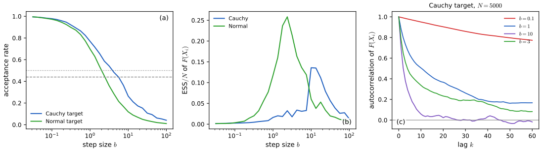
fig_24_s4. Download: PDF · SVGFilling the gap 24.14: transforming a restricted variable needs the Jacobian p. 415
If \(X>0\) has density \(f_X\) and we run the random walk on \(W=\log X\), the chain must target the density of \(W\), which by the change-of-variables formula (Result 2.17) is
\[f_W(w)=f_X(e^w)\,e^w.\]Forgetting the factor \(e^w\) samples the wrong distribution. Equivalently, one may stay on the original scale with the multiplicative proposal \(Y=Xe^{bZ}\): its density is \(q(y\given x)=\phi(\log(y/x)/b)/(by)\), so \(q(x\given y)/q(y\given x)=y/x\), and the Hastings factor \(y/x\) is exactly the Jacobian. Exercise 24.4(b) uses this; the demonstration's last preset runs it.
Independence Metropolis-Hastings. p. 415 The proposal is drawn from a fixed density \(g\), chosen to approximate \(f\); then
\[r(x,y)=\min\Big\{1,\ \frac{f(y)}{f(x)}\,\frac{g(x)}{g(y)}\Big\}=\min\Big\{1,\ \frac{w(y)}{w(x)}\Big\},\qquad w=\frac fg,\]the ratio of the importance weights of the proposal and the current point: an importance-sampling version of MCMC.
Filling the gap 24.15: when the independence sampler works, and when it gets stuck
If \(f\le Mg\) for a constant \(M\) (the proposal has heavier tails than the target), the chain converges geometrically from any starting point: \(\|P^n(x,\cdot)-f\|_{\TV}\le(1-1/M)^n\) (Mengersen and Tweedie 1996). The bound is confirmed numerically on a finite example.
Proof
Since \(w\le M\), \(\min\{1,w(y)/w(x)\}\)
If \(g\) has lighter tails than \(f\), \(w=f/g\) is unbounded. When the chain reaches a point with a large weight \(w(x)\), every proposal \(y\) with \(w(y)\ll w(x)\) is rejected, and the chain stays for a long time; the far tails are rarely proposed at all. The chain is then not geometrically ergodic (Mengersen and Tweedie 1996), and averages converge slowly and erratically. For a Cauchy target and a \(\N(0,1)\) proposal, a chain of 5000 spends 4% of its time beyond \(\pm3\), where the target has 20% of its mass. This is the MCMC counterpart of the infinite-variance importance sampler of Filling the gap 24.6.
Gibbs sampling
pp. 415–418 Gibbs sampling turns a high-dimensional problem into a sequence of low-dimensional ones by sampling each coordinate from its conditional distribution given the others.
Algorithm 24.B (Gibbs sampling) p. 416
For a pair \((X,Y)\) with density \(f_{X,Y}\), start at \((X_0,Y_0)\) and repeat
\[X_{n+1}\sim f_{X\given Y}(x\given Y_n),\qquad Y_{n+1}\sim f_{Y\given X}(y\given X_{n+1}).\]With more coordinates, each is drawn in turn from its conditional given the most recent values of all the others.
Result 24.D (Gibbs sampling is Metropolis–Hastings that always accepts)
The update of \(X\) with \(Y=y\) fixed is a Metropolis-Hastings step with proposal \(q(x'\given x,y)=f_{X\given Y}(x'\given y)\), and its acceptance probability is 1. Each update leaves \(f_{X,Y}\) invariant, and so does a sweep through all coordinates.
Filling the gap 24.16: proof of Result 24.D
Proof
Acceptance 1. The move is \((x,y)\to(x',y)\) with proposal density \(f(x'\given y)\), and the reverse move has density \(f(x\given y)\). The Hastings ratio is
\[\frac{f(x',y)}{f(x,y)}\cdot\frac{f(x\given y)}{f(x'\given y)}=\frac{f_Y(y)f(x'\given y)}{f_Y(y)f(x\given y)}\cdot\frac{f(x\given y)}{f(x'\given y)}=1.\]Invariance. Directly: if \((X,Y)\sim f\) and \(X'\given(X,Y)\sim f(\cdot\given Y)\), then \((X',Y)\) has density \(\int f(x,y)f(x'\given y)\,\d x\)
A systematic sweep is not itself reversible, but invariance is all the ergodic theorem needs, together with irreducibility. Irreducibility can fail: if \(f\) is uniform on two squares touching only at a corner, \((0,1)^2\cup(1,2)^2\), every conditional stays in the current square and the Gibbs sampler never crosses. Strong correlation slows it down in the same way, gradually (the companion courses show this for a bivariate Normal).
See also Result 8.10 of Statistical Learning: Theory and Methods, Result 11.20 of Bayesian and Probabilistic Machine Learning and Result 14.10 of Foundations of Deep Learning.
Example 24.11 (a hierarchical model). pp. 416–418 In each of \(k\) cities, \(n_i\) people are sampled and \(Y_i\sim\Bin(n_i,p_i)\) have a disease; the rates \(p_i\) are themselves draws from a population distribution, whose centre is the overall disease rate. Work on the log-odds scale: \(\psi_i=\logit p_i\), estimated by \(Z_i=\logit\hat p_i\) with \(\hat p_i=Y_i/n_i\). By the delta method (Theorem 5.13) \(Z_i\approx\N(\psi_i,\sigma_i^2)\) with \(\sigma_i^2=1/(n_i\hat p_i(1-\hat p_i))\), treated as known. The model is
\[\psi_i\sim\N(\mu,\tau^2),\qquad Z_i\given\psi_i\sim\N(\psi_i,\sigma_i^2),\]with \(\tau=1\) and a flat prior on \(\mu\). The unknowns are \(\th=(\mu,\psi_1,\dots,\psi_k)\), and the posterior is proportional to
\[\prod_i\exp\Big(-\frac12(\psi_i-\mu)^2\Big)\exp\Big(-\frac1{2\sigma_i^2}(Z_i-\psi_i)^2\Big).\]The full conditionals (Filling the gap 24.17) are \(\mu\given\rest\sim\N(\bar\psi,1/k)\) with \(\bar\psi=k^{-1}\sum\psi_i\), and \(\psi_i\given\rest\sim\N(e_i,d_i^2)\) with
\[e_i=\frac{Z_i/\sigma_i^2+\mu}{1+1/\sigma_i^2},\qquad d_i^2=\frac1{1+1/\sigma_i^2}.\]The Gibbs sampler draws \(\mu\), then \(\psi_1,\dots,\psi_k\), each from its conditional given the latest values, and repeats. We simulated \(k=20\) cities of \(n=20\) people with \(\psi_i\sim\N(0,1)\) (counts 7, 8, 11, 18, 2, 18, 17, 13, 2, 7, 8, 12, 14, 6, 17, 9, 18, 13, 17, 6), ran 1000 iterations and converted each \(\psi_i\) back to \(p_i=e^{\psi_i}/(1+e^{\psi_i})\). The posterior of \(\mu\) has mean 0.27 and standard deviation 0.26, which the sampler reproduces; the Bayes estimates of the \(p_i\) are pulled towards the centre (their spread is 0.19 against 0.26 for the raw proportions), most strongly for the extreme cities, where \(\sigma_i^2\) is largest.
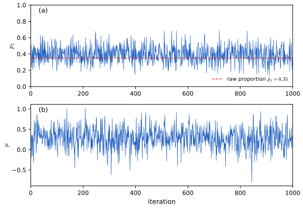
fig_24_3. Download: PDF · SVG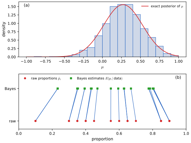
fig_24_4. Download: PDF · SVGFilling the gap 24.17: the full conditionals, and the exact posterior that checks the sampler pp. 416–417
We keep \(\tau\) general. Dropping every factor that does not contain \(\mu\), \(f(\mu\given\rest)\propto\exp\big(-\frac1{2\tau^2}\sum_i(\psi_i-\mu)^2\big)\)
so \(\psi_i\given\rest\sim\N(e_i,d_i^2)\) with \(d_i^2=1/(1/\sigma_i^2+1/\tau^2)\): the precision-weighted average of the city's own estimate and the population mean.
The exact posterior. This model is simple enough to solve exactly, which is the best way to test a sampler. Integrating \(\psi_i\) out, \(Z_i\given\mu\sim\N(\mu,\sigma_i^2+\tau^2)\) independently, so with a flat prior
\[\mu\given Z\sim\N\Big(\frac{\sum_iv_iZ_i}{\sum_iv_i},\ \frac1{\sum_iv_i}\Big),\quad v_i=\frac1{\sigma_i^2+\tau^2};\qquad \E(\psi_i\given Z)=B_i\,\E(\mu\given Z)+(1-B_i)Z_i,\quad B_i=\frac{\sigma_i^2}{\sigma_i^2+\tau^2}.\]The shrinkage factor \(B_i\) is largest for cities with the noisiest estimates: with \(n=20\), \(B_i=0.17\) for \(\hat p_i=0.5\) but 0.36 for \(\hat p_i=0.1\). For our data \(\E(\mu\given Z)=0.271\) and \(\mathrm{sd}=0.256\); a long Gibbs run agrees to Monte Carlo accuracy for \(\mu\) and every \(\psi_i\). As the book says, \(\tau\) should really be estimated too; giving it a prior adds one more conditional, an inverse-gamma for \(\tau^2\) under a conjugate prior.
Metropolis within Gibbs, and convergence diagnostics
pp. 418–419 When a conditional cannot be sampled directly, replace the exact draw by a Metropolis-Hastings step that targets it.
Algorithm 24.C (Metropolis within Gibbs) p. 419
With proposals \(q\) for \(x\) and \(\tilde q\) for \(y\):
- (1a) draw \(Z\sim q(z\given X_n)\); (1b) compute \(r=\min\Big\{\dfrac{f(Z,Y_n)}{f(X_n,Y_n)}\dfrac{q(X_n\given Z)}{q(Z\given X_n)},1\Big\}\); (1c) set \(X_{n+1}=Z\) with probability \(r\), else \(X_{n+1}=X_n\);
- (2a) draw \(Z\sim\tilde q(z\given Y_n)\); (2b) compute \(r=\min\Big\{\dfrac{f(X_{n+1},Z)}{f(X_{n+1},Y_n)}\dfrac{\tilde q(Y_n\given Z)}{\tilde q(Z\given Y_n)},1\Big\}\); (2c) set \(Y_{n+1}=Z\) with probability \(r\), else \(Y_{n+1}=Y_n\).
Filling the gap 24.18: why Metropolis within Gibbs is valid p. 419
In step 1, \(f(Z,Y_n)/f(X_n,Y_n)=f(Z\given Y_n)/f(X_n\given Y_n)\): the unknown marginal \(f_Y(Y_n)\) cancels. So step 1 is exactly a Metropolis-Hastings step for the conditional density \(f(\cdot\given Y_n)\), and by Theorem 24.C its kernel \(K_y\) leaves \(f(\cdot\given y)\) invariant. Then, as in Filling the gap 24.16 with \(f(x'\given y)\) replaced by \(K_y\),
\[\int f(x,y)K_y(x,x')\,\d x=f_Y(y)\int f(x\given y)K_y(x,x')\,\d x=f_Y(y)f(x'\given y)=f(x',y),\]so the step leaves the joint \(f\) invariant, and so does step 2 and their composition. One Metropolis step per coordinate is enough: the conditional need not be reached exactly, only left invariant. Exercise 24.5 uses this for a logistic regression.
Filling the gap 24.19: how do we know a chain has converged?
We cannot know; we can only look for evidence that it has not. The standard checks:
- Trace plots (Figures 24.2, 24.3): a converged chain looks like stationary noise around a fixed level, with no trend and no long stuck stretches.
- Burn-in: discard an initial stretch while the chain forgets its starting value. By the ergodic theorem this does not change the limit, only the finite-\(N\) bias.
- Several chains from dispersed starting values. With \(m\) chains of length \(n\), let \(W\) be the average within-chain variance and \(B/n\) the variance of the chain means. Gelman and Rubin (1992) compare \(\hat V=\frac{n-1}nW+\frac Bn\), which overestimates the target variance while the chains still remember their starts, with \(W\), which underestimates it, through
- Values near 1 (below 1.01 is a common modern threshold) are consistent with convergence; values well above 1 show that the chains have not yet mixed. For Example 24.11, four chains started at \(\mu=\psi_i=-6,-2,2,6\) agree within a few iterations, and \(\Rhat\) is below 1.01 after 200 (Figure 24.S5).
- The effective sample size (Filling the gap 24.12) says how precise the estimates are once the chain has converged.
None of these can detect a mode that no chain has found: a two-mode target sampled with small steps can pass every test while missing half the mass.
Why \(\Rhat\to1\)
For stationary chains, \(\E W\to\sigma^2\) and \(B/n=\) the variance of \(m\) chain means, each with variance about \(\sigma^2\tau/n\to0\); so \(\hat V\to\sigma^2\) and \(\Rhat\to1\) as \(n\to\infty\). While the chains still depend on their dispersed starts, the chain means differ by \(O(1)\) amounts, \(B/n\) stays of order 1, and \(\hat V>W\), so \(\Rhat>1\). ∎
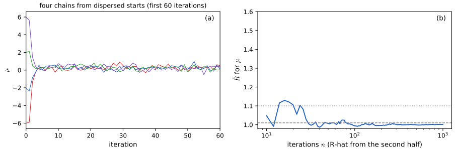
fig_24_s5. Download: PDF · SVG24.6 Bibliographic Remarks
p. 420 MCMC began with the work of Metropolis et al. (1953) on the computation of physical equilibria, was generalised by Hastings (1970), was used in spatial statistics and image analysis (Geman and Geman 1984 named the Gibbs sampler), and entered mainstream statistics with Gelfand and Smith (1990). The book's main reference is Robert and Casella (1999); see also Gelman et al. (1995) and Gilks et al. (1998). For the theory used in these notes: Tierney (1994) and Roberts and Rosenthal (2004) on convergence, Mengersen and Tweedie (1996) on the independence and random-walk samplers, Geyer (1992) on estimating the autocorrelation time, Kong (1992) on the effective sample size, and Roberts, Gelman and Gilks (1997) on optimal scaling.
Notes on the book
Four slips of Chapter 24 are in the author's errata lists; the other points are mine, each with the evidence. The two most consequential are the dose-response numbers of Example 24.4 and the quantities called variances in Example 24.6.
Page 406, Example 24.3: the displayed integrals are missing \(\d p_1\,\d p_2\)
Listed in the author's errata (item 65 of the first list).
Page 407, Example 24.4: \(Y_i\) is the number of deaths, not of survivors
The text says \(Y_i\) is "the number that survive" with \(Y_i\sim\Bin(n,p_i)\), while \(p_i\) is the probability of death (higher doses, higher \(p_i\), and the LD50 is where \(p_i\) reaches 1/2). The data (0, 0, 2, 2, 8, 10, 12, 14, 15, 14 of 15) increase with the dose, and the sampler draws \(p_i\sim\Beta(Y_i+1,n-Y_i+1)\): both only make sense if \(Y_i\) counts deaths. Not in the errata lists.
Page 408, Example 24.4: "\(\hat\delta=4.04\) with a 95 percent interval of (3, 5)" cannot come from these data
Running the book's algorithm on the book's data gives a posterior mean of 5.58 and a 95% interval \((5,7)\) (20,000 kept draws; Figure 24.S2). A value near 4 would need \(\P(\delta\le4\given Y)\) to be large, but it is about 0.002: \(\delta\le4\) requires \(P_4>1/2\), while the unconstrained posterior of \(p_4\) is \(\Beta(3,14)\), for which \(\P(p_4>1/2)\approx0.006\), and the ordering constraint barely changes this. Counting doses from 0 instead of 1 gives 4.58, still not 4.04. Not in the errata lists.
Page 408: "the second panel in the figure" does not exist
Listed in the author's errata (item 66 of the first list: ignore the phrase). Figure 24.S2(a) shows what such a panel would contain.
Page 409, proof of Theorem 24.5: \((\E(w^2))^2\) should be \((\E_g(w))^2\)
Listed in the author's errata (item 67 of the first list). See Filling the gap 24.7.
Page 410, Example 24.6: the reported "variances" are standard deviations
For plain Monte Carlo with \(N=100\) the exact variance is \(I(1-I)/100=1.35\times10^{-5}\), whose square root \(0.0037\) is the book's "\(\V(\hI)=.0039\)"; for the \(\N(4,1)\) proposal the exact standard deviation is \(0.00031\) (Filling the gap 24.6), the book's ".0002". The final sentence ("reduced the standard deviation by a factor of 20") confirms the reading; the exact factor is 12. The book's simulated mean \(.0011\) for the importance sampler is also off: with standard deviation 0.0003, the average of many repetitions should be within a few \(10^{-5}\) of \(0.00135\) (10,000 repetitions give \(0.001348\)). Not in the errata lists.
Page 410, Example 24.7: the \(t\) density needs \(1/\sqrt{\nu\pi}\), not \(1/(\nu\pi)\)
The author's second errata list (item 2) corrects the same missing square root in the \(t\) density on page 30; the copy in Example 24.7 has the same slip. The normalising constant cancels in the posterior mean, so the example's numbers are unaffected.
Page 410, Example 24.7: \(X_i\sim N(\th_i,1)\) should be \(N(\th,1)\)
All measurements share the one quantity \(\th\). Not in the errata lists. The example also does not give its two observations; since the posterior is symmetric about their average (Filling the gap 24.8), the stated posterior mean \(-0.54\) is their average.
Page 411: Theorem 23.25 covers countable state spaces and bounded \(h\)
MCMC chains here live on \(\R\) or \(\R^k\), and \(h(x)=x\) is unbounded. The law of large numbers needed is the general ergodic theorem for \(f\)-irreducible chains (Filling the gap 24.11). Not an error, a gap.
Page 412, Remark 24.8: "\(U\sim(0,1)\)" should be \(U\sim\Unif(0,1)\)
A typographical slip. Not in the errata lists.
Pages 412–413, Example 24.10: \(b=10\) is better than \(b=1\) for the Cauchy target
The book concludes that the middle chain "better represents the density sooner". Averaged over 100 chains of length 1000 started at 0, the Kolmogorov-Smirnov distance between the chain's empirical cdf and the Cauchy cdf is 0.31, 0.125 and 0.094 for \(b=0.1\), 1 and 10, and the effective sample size of \(F(X_i)\) is 8, 38 and 126. The stuck stretches of the \(b=10\) chain are visible, but the slow tail excursions of the \(b=1\) chain cost more (Filling the gap 24.13, Figure 24.S4). A matter of judgement rather than an error; not in the errata lists.
Page 415: the 50 percent rule of thumb
Theory gives 0.44 for one-dimensional Normal targets and 0.234 in high dimensions (Roberts, Gelman and Gilks 1997); for the Cauchy the best rate is near 0.3. 50% is a reasonable rough guide in low dimensions (Filling the gap 24.13). Not an error.
Pages 416–417, Example 24.11: \(\sigma_i^2\) and the variance of \(\mu\)
The delta-method variance should read \(\sigma_i^2=1/(n_i\hat p_i(1-\hat p_i))\), with the city's own sample size and the estimated proportion (it is "treated as known", so it cannot involve the unknown \(p_i\)); and in the boxed algorithm "draw \(\mu\sim N(b,v^2)\)" should be \(N(b,1/k)\), as derived just above it. Not in the errata lists. See Filling the gap 24.17.
Page 418, caption of Figure 24.3: the second "top panel" should be "bottom panel"
The caption says twice that the top panel shows the simulated values; the second sentence describes \(\mu\), which is in the bottom panel. Not in the errata lists.
Page 421, Exercise 3(b): the Cauchy density is \(1/(\pi(1+x^2))\)
The exercise calls \(g(x)=1/(1+x^2)\) "the Cauchy density"; it integrates to \(\pi\). The method still works with an unnormalised \(g\) (the constant \(M\) absorbs \(\pi\)), but with the density as written in the exercise the bound would be \(M=\sqrt{2\pi/e}/\pi\). Not in the errata lists.
Page 422, Exercise 5: the first part should begin "(a) Use ..."
Listed in the author's errata (item 68 of the first list).
24.7 Exercises
All five exercises of Chapter 24 (Wasserman, 2004, pp. 420–422), restated in my own words, with complete solutions (hidden). The computations are in the Python code (functions ex1 to ex5).
Exercise 24.1. Let \(I=\int_1^2\phi(x)\,\d x\). (a) Estimate \(I\) by basic Monte Carlo with \(N=100{,}000\), with its estimated standard error. (b) Find the exact standard error of the estimate in (a) and compare. (c) Estimate \(I\) by importance sampling with \(g=\N(1.5,v^2)\) for \(v=0.1\), 1 and 10; compute the exact standard errors, and look at a histogram of the terms being averaged for extreme values. (d) Find the optimal importance density \(g^*\) and its standard error.
Solution
The exact value is \(I=\Phi(2)-\Phi(1)=0.135905\).
(a) With \(X_i\sim\Unif(1,2)\) and \(w(x)=\phi(x)\) (here \(b-a=1\)), 100,000 draws give \(\hI=0.135942\) with \(\hse=1.747\times10^{-4}\).
(b) \(\V(\phi(X))=\int_1^2\phi^2-I^2\). Since \(\phi(x)^2=\frac1{2\sqrt\pi}\cdot\frac1{\sqrt{2\pi}\,(1/\sqrt2)}e^{-x^2}\) is \(1/(2\sqrt\pi)\) times the \(\N(0,1/2)\) density,
\[\int_1^2\phi^2=\frac{\Phi(2\sqrt2)-\Phi(\sqrt2)}{2\sqrt\pi}=0.021526,\qquad\se=\sqrt{\frac{0.021526-I^2}{N}}=1.748\times10^{-4},\]which the estimate in (a) matches to within 0.1%. (Estimating \(I\) instead as the proportion of \(\N(0,1)\) draws in \((1,2)\) has \(\se=\sqrt{I(1-I)/N}=1.08\times10^{-3}\), six times larger.)
(c) The terms are \(\ind\{1<X<2\}\phi(X)/g(X)\), and the exact standard error is \(\sqrt{(\int_1^2\phi^2/g-I^2)/N}\), computed by quadrature:
\(v\) estimate exact se largest term 0.1 0.1265 \(2.9\times10^{-2}\) 1603 1 0.13528 \(6.2\times10^{-4}\) 0.69 10 0.13554 \(2.3\times10^{-3}\) 6.1 With \(v=0.1\) the proposal is far too narrow: near \(x=1\) the density \(g\) is \(e^{-12.5}\) times its peak while \(\phi\) is not small, so a rare draw there carries a weight of order 1000 (Figure 24.S6(a)); the variance is finite only because the interval is bounded. With \(v=10\) most draws fall outside \((1,2)\) and are wasted. \(v=1\) is the best of the three, yet still worse than the uniform proposal of (a), which is already close to \(g^*\) in shape.
(d) By Theorem 24.5 (with \(h=\ind_{(1,2)}\ge0\)), \(g^*(x)=\phi(x)\ind\{1<x<2\}/I\), the Normal truncated to \((1,2)\). Every term equals \(\phi/g^*=I\), so the standard error is 0. (It can be sampled by inversion, \(X=\Phi^{-1}(\Phi(1)+UI)\), which needs \(I\): the usual catch.)
▶ DemoExercise 24.1(c) with v = 0.1Then move the scale to 1 and 10, and try the optimal g* (preset 7).Exercise 24.2. Importance sampling for a marginal density. Let \((X_1,Y_1),\dots,(X_N,Y_N)\) be drawn from \(f_{X,Y}\) and let \(w\) be any probability density. (a) Show that, for each \(x\),
\[\hat f_X(x)=\frac1N\sum_{i=1}^N\frac{f_{X,Y}(x,Y_i)\,w(X_i)}{f_{X,Y}(X_i,Y_i)}\ \xrightarrow{\ \P\ }\ f_X(x),\]and find its variance. (b) Apply it with \(Y\sim\N(0,1)\) and \(X\given Y=y\sim\N(y,1+y^2)\).
Solution
(a) The terms \(T_i=f(x,Y_i)w(X_i)/f(X_i,Y_i)\) are iid, and (on \(\{f>0\}\))
\[\E\,T_i=\iint\frac{f(x,y)w(x')}{f(x',y)}f(x',y)\,\d x'\,\d y=\int f(x,y)\,\d y\int w(x')\,\d x'=f_X(x).\]So \(\hat f_X(x)\) is unbiased and, by the weak law, consistent. Its variance is \(\V(T_1)/N\), with
\[\V(T_1)=\iint\frac{f(x,y)^2\,w(x')^2}{f(x',y)}\,\d x'\,\d y-f_X(x)^2.\]It is finite when \(w\) has lighter tails than \(f(\cdot,y)\) in \(x'\); the variance is smallest when \(w(x')\) is close to \(f(x'\given y)\) (with \(w(x')=f_{X\given Y}(x'\given y)\) for every \(y\) the ratio becomes \(f(x\given y)\) and the estimator is the average of the conditional densities, the "Rao-Blackwellised" estimator). The joint density enters only through the ratio \(f(x,Y_i)/f(X_i,Y_i)\), so its normalising constant cancels: the method works for densities known up to a constant, such as posteriors.
(b) Here \(f(x,y)=\phi(y)\,\phi\big((x-y)/\sqrt{1+y^2}\big)\)
\({}/\sqrt{1+y^2}\). With \(w=\N(0,2)\) and \(N=1000\) the estimate tracks the exact marginal (computed by quadrature) closely across \(x\in(-6,6)\): for example \(\hat f_X(0)=0.280\) (sd 0.011) against 0.2752, and \(\hat f_X(2)=0.0952\) (sd 0.004) against 0.0954 (Figure 24.S6(b)). The marginal is symmetric with heavier tails than any Normal, since it is a scale mixture. Exercise 24.3. Accept-reject sampling. (a) Let \(f\) and \(g\) be densities with \(f\le Mg\) for a known \(M\). Draw \(X\sim g\) and \(U\sim\Unif(0,1)\); if \(U\le f(X)/(Mg(X))\) set \(Y=X\), otherwise repeat. Show that \(Y\sim f\). (b) Use it with \(f=\phi\) and \(g\) the Cauchy density to draw 1000 Normal observations and check them with a histogram.
Solution
(a) One round accepts with probability \(\P(U\le f(X)/(Mg(X)))\)
\[\P(Y\le t)=\frac{\P\big(X\le t,\ U\le f(X)/(Mg(X))\big)}{1/M}=M\int_{-\infty}^tg(x)\frac{f(x)}{Mg(x)}\,\d x=\int_{-\infty}^tf(x)\,\d x.\]\({}=\int g(x)\frac{f(x)}{Mg(x)}\,\d x=\frac1M\). The rounds are independent, so the accepted value has the distribution of \(X\) given acceptance: The number of rounds is geometric with mean \(M\). (The condition \(f\le Mg\) needs \(g>0\) wherever \(f>0\).)
(b) With \(g(x)=1/(\pi(1+x^2))\), \(\phi(x)/g(x)=\sqrt{\pi/2}\,(1+x^2)e^{-x^2/2}\), whose derivative vanishes where \(2x-x(1+x^2)=0\), i.e. at \(x=0,\pm1\); the maximum is at \(\pm1\), giving \(M=\sqrt{\pi/2}\cdot2e^{-1/2}=\sqrt{2\pi/e}=1.520\). The acceptance rate is \(1/M=0.658\); 1000 accepted draws took 1518 proposals (rate 0.659), and the histogram matches \(\phi\) (Figure 24.S6(c); a Kolmogorov-Smirnov test does not reject normality). Cauchy draws are \(\tan(\pi(V-1/2))\) with \(V\) uniform (inverse cdf, Result 2.4).
See also Result 11.7 of Bayesian and Probabilistic Machine Learning and Result 14.3 of Foundations of Deep Learning.
Exercise 24.4. The inverse Gaussian density is
\[f(z)\propto z^{-3/2}\exp\big(-\th_1z-\th_2/z+2\sqrt{\th_1\th_2}+\log\sqrt{2\th_2}\big),\quad z>0,\]with \(\E Z=\sqrt{\th_2/\th_1}\) and \(\E(1/Z)=\sqrt{\th_1/\th_2}+1/(2\th_2)\). With \(\th_1=1.5\), \(\th_2=2\): (a) draw 1000 values by independence Metropolis-Hastings with a Gamma proposal, and judge the accuracy by comparing the sample means of \(Z\) and \(1/Z\) with the exact ones, for several Gamma proposals; (b) do the same with random-walk Metropolis-Hastings on \(W=\log Z\), after finding the density of \(W\).
Solution
The density and the moments. This is the inverse Gaussian with mean \(\mu=\sqrt{\th_2/\th_1}\) and shape \(\lambda=2\th_2\): expanding \(\sqrt{\lambda/(2\pi z^3)}\exp(-\lambda(z-\mu)^2/(2\mu^2z))\) gives the exponent \(-\frac\lambda{2\mu^2}z+\frac\lambda\mu-\frac\lambda{2z}=-\th_1z+2\sqrt{\th_1\th_2}-\th_2/z\), and the constant is \(\sqrt{\th_2/\pi}\). So \(\E Z=\mu=1.1547\) and \(\E(1/Z)=1/\mu+1/\lambda\)
\({}=0.8660+0.25=1.1160\) (both confirmed by quadrature). (a) With proposal \(g=\mathrm{Gamma}(a,\text{rate }r)\), the acceptance probability is \(\min\{1,w(y)/w(x)\}\) with \(w=f/g\). The moment-matched Gamma (\(\mu^2/\V Z=3.46\), rate \(\mu/\V Z=3\), using \(\V Z=\mu^3/\lambda=0.385\)) accepts 89% of proposals and gives means 1.135 and 1.133 from 1000 draws; \(\mathrm{Gamma}(1,1)\) (an exponential, heavier-tailed) accepts 55% and gives 1.128 and 1.121; \(\mathrm{Gamma}(20,20)\), concentrated near 1 with sd 0.22, gives 1.212 and 0.996: its tails are too light on both sides, so the chain sticks whenever it reaches a tail value, the situation of Filling the gap 24.15. The first two are accurate to within their Monte Carlo error (about 0.03 with 1000 correlated draws).
(b) By Filling the gap 24.14, \(f_W(w)=f(e^w)e^w\)
\({}\propto\exp\big(-\tfrac w2-\th_1e^w-\th_2e^{-w}\big)\), a density on all of \(\R\). Random-walk Metropolis with \(b=1\) accepts 51% and, after \(Z_i=e^{W_i}\), gives means 1.083 and 1.146 from 1000 draws, within about two Monte Carlo standard errors of the exact values; with 20,000 draws both are within 3% of the exact values. Figure 24.S7 (left) compares the samples with the density. ▶ DemoExercise 24.4(b): the random walk on log ZThe histogram is on the W scale, with the Jacobian included in the target.Exercise 24.5. For the heart disease data of the book's website, consider a Bayesian logistic regression \(\P(Y=1\given X=x)=\expit(\beta_0+\sum_{j=1}^k\beta_jx_j)\) with the flat prior \(f(\beta_0,\dots,\beta_k)\propto1\). (a) Use the Metropolis-within-Gibbs algorithm to draw 10,000 values from the posterior, plot histograms of the posteriors of the \(\beta_j\), and report each posterior mean and 95% posterior interval. (b) Compare with the maximum likelihood analysis.
Solution
Data and model. The heart disease data are the South African coronary risk factor study (CORIS) of the book's Example 13.17 (notes): 462 men, response chd, nine covariates. The log-posterior is the log-likelihood \(\sum_i[y_i\eta_i-\log(1+e^{\eta_i})]\), \(\eta_i=\beta_0+x_i^\T\beta\). The flat prior gives a proper posterior here because the MLE exists (the data are not separable) and the log-likelihood is strictly concave and tends to \(-\infty\) in every direction.
Sampler. Each sweep updates \(\beta_0,\dots,\beta_9\) in turn by a random-walk Metropolis step (Algorithm 24.C) with the others held fixed, updating the linear predictor in place, so a sweep costs \(O(nk)\). For good mixing the chain runs on standardised covariates (a linear reparametrisation, under which a flat prior stays flat) with step sizes \(2.4\) times the MLE standard errors in that scale; the draws are mapped back to the original units. After 1000 sweeps of burn-in, 10,000 sweeps are kept; acceptance rates are 0.27 to 0.44, and the effective sample sizes range from about 400 (adiposity, obesity, which are strongly correlated) to 1900.
coef. posterior mean
(95% interval)MLE
(se)intercept −6.360
(−8.995, −3.799)−6.151
(1.308)sbp 0.0069
(−0.0044, 0.0190)0.0065
(0.0057)tobacco 0.0825
(0.0317, 0.1363)0.0794
(0.0266)ldl 0.178
(0.061, 0.304)0.174
(0.060)adiposity 0.019
(−0.039, 0.078)0.019
(0.029)famhist 0.952
(0.488, 1.420)0.925
(0.228)typea 0.0413
(0.0173, 0.0660)0.0396
(0.0123)obesity −0.065
(−0.157, 0.021)−0.063
(0.044)alcohol 0.0001
(−0.0087, 0.0087)0.0001
(0.0045)age 0.0460
(0.0225, 0.0708)0.0452
(0.0121)(b) The MLE (Newton-Raphson, agreeing with a standard library fit) and its Wald intervals \(\hat\beta_j\pm1.96\,\hse\) lead to the same conclusions: tobacco, ldl, family history, type-A behaviour and age are clearly associated with heart disease; blood pressure, adiposity, obesity and alcohol are not. The posterior means are within a quarter of a posterior standard deviation of the MLE, slightly further from zero, and the posterior standard deviations are up to 5% larger than the standard errors: the Bernstein-von Mises theorem (Theorem 11.5) at work with \(n=462\) and ten parameters. The posterior histograms are close to the Normal approximations \(\N(\hat\beta_j,\hse^2)\) (Figure 24.S7).
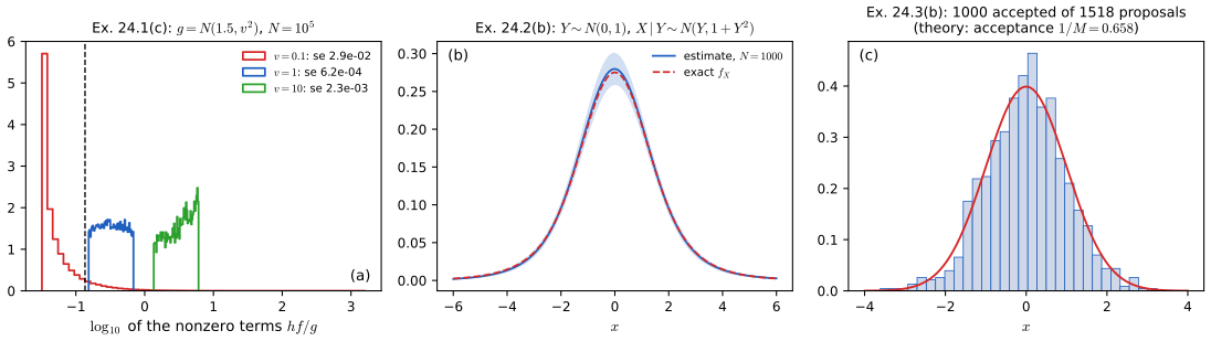
fig_24_s6. Download: PDF · SVG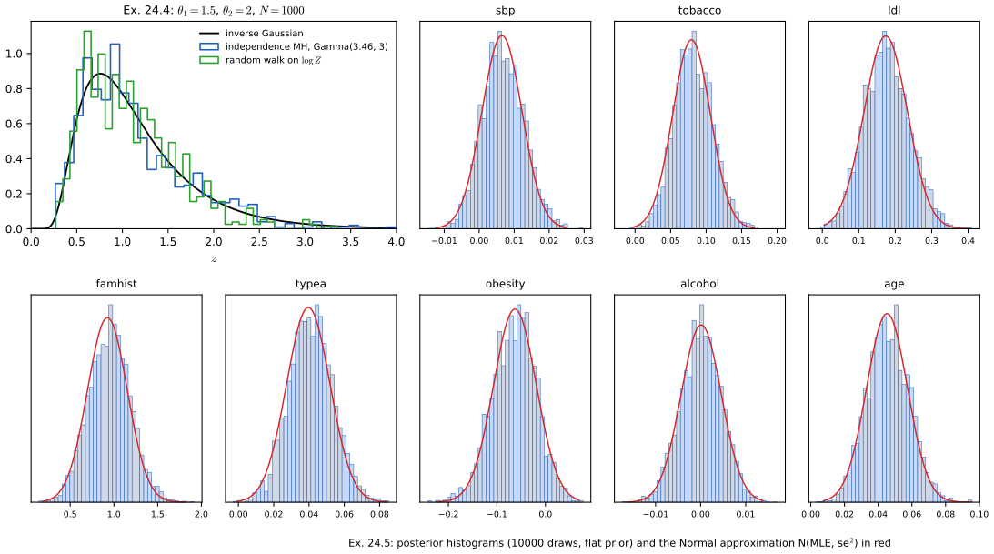
fig_24_s7. Download: PDF · SVGDemonstrations for this chapter
Each demonstration runs in the browser and links back to these notes. The ▶ Demo boxes above open them already set to the case under discussion.
| Demonstration | What you can see | Sections and results |
|---|---|---|
| Monte Carlo integration: the error shrinks like 1/√N | One run with its estimated interval as \(N\) grows; the spread of up to 500 runs against \(\sigma/\sqrt N\) on log scales; the histogram of the estimates against the Normal approximation; the intervals of the first 40 runs and the coverage. Presets: 1 Example 24.1; 2 Example 24.2; 3 Example 24.2 with \(N=10^5\); 4 a rare event; 5 Example 24.3. | 24.2; Theorem 24.A; Filling the gaps 24.2, 24.4 |
| Importance sampling: why the proposal needs heavy tails | The target and a Normal, \(t_3\), Cauchy or optimal proposal, with weighted draws; one run's estimate as \(N\) grows; 200 runs against the exact variance, which can be infinite; the effective sample size and the largest weight. Presets: 1 plain Monte Carlo for \(\P(Z>3)\); 2 the \(\N(4,1)\) proposal; 3 too narrow; 4 Example 24.7, Normal; 5 Example 24.7, Cauchy; 6 Exercise 24.1(c); 7 the optimal \(g^*\). | 24.3; Theorems 24.B, 24.5; Filling the gaps 24.6, 24.8; Definition 24.A |
| Tuning Metropolis-Hastings | A random-walk or independence chain for a Cauchy, Normal, two-mode or inverse Gaussian target: trace, histogram, autocorrelation, effective sample size and KS distance, and the acceptance rate and ESS/\(N\) over 29 step sizes. Presets: 1–3 the chains of Figure 24.2; 4 the optimal step for a Normal; 5 two modes; 6 an independence sampler with light tails; 7 Exercise 24.4(b). | 24.4, 24.5; Algorithm 24.A; Filling the gaps 24.12–24.15 |
Related demonstrations in the companion courses: the sampling basics, MCMC (Metropolis and Gibbs on a correlated Gaussian) and slice sampling and HMC demos of Bayesian and Probabilistic Machine Learning, and the Langevin sampling demo of Foundations of Deep Learning. In this course, the Chapter 2 inverse-cdf sampling demo shows how the uniform draws become draws from a given distribution. The Python code that produces every figure of this page is code/ch24_simulation_methods.py (see the code index).
References
- Wasserman, L. (2004). All of Statistics: A Concise Course in Statistical Inference. Springer, New York. Chapter 24, pp. 403–422. www.stat.cmu.edu/~larry/all-of-statistics.
- Gelfand, A. E. and Smith, A. F. M. (1990). Sampling-based approaches to calculating marginal densities. Journal of the American Statistical Association, 85(410), 398–409.
- Gelman, A., Carlin, J. B., Stern, H. S. and Rubin, D. B. (1995). Bayesian Data Analysis. Chapman and Hall, London.
- Gelman, A., Roberts, G. O. and Gilks, W. R. (1996). Efficient Metropolis jumping rules. In Bayesian Statistics 5, 599–607. Oxford University Press.
- Gelman, A. and Rubin, D. B. (1992). Inference from iterative simulation using multiple sequences. Statistical Science, 7(4), 457–472.
- Geman, S. and Geman, D. (1984). Stochastic relaxation, Gibbs distributions, and the Bayesian restoration of images. IEEE Transactions on Pattern Analysis and Machine Intelligence, 6(6), 721–741.
- Geyer, C. J. (1992). Practical Markov chain Monte Carlo. Statistical Science, 7(4), 473–483.
- Gilks, W. R., Richardson, S. and Spiegelhalter, D. J. (eds.) (1998). Markov Chain Monte Carlo in Practice. Chapman and Hall, London.
- Hastings, W. K. (1970). Monte Carlo sampling methods using Markov chains and their applications. Biometrika, 57(1), 97–109.
- Jarner, S. F. and Tweedie, R. L. (2003). Necessary conditions for geometric and polynomial ergodicity of random-walk-type Markov chains. Bernoulli, 9(4), 559–578.
- Kong, A. (1992). A note on importance sampling using standardized weights. Technical Report 348, Department of Statistics, University of Chicago.
- Mengersen, K. L. and Tweedie, R. L. (1996). Rates of convergence of the Hastings and Metropolis algorithms. The Annals of Statistics, 24(1), 101–121.
- Metropolis, N., Rosenbluth, A. W., Rosenbluth, M. N., Teller, A. H. and Teller, E. (1953). Equation of state calculations by fast computing machines. The Journal of Chemical Physics, 21(6), 1087–1092.
- Robert, C. P. and Casella, G. (1999). Monte Carlo Statistical Methods. Springer, New York.
- Roberts, G. O., Gelman, A. and Gilks, W. R. (1997). Weak convergence and optimal scaling of random walk Metropolis algorithms. The Annals of Applied Probability, 7(1), 110–120.
- Roberts, G. O. and Rosenthal, J. S. (2004). General state space Markov chains and MCMC algorithms. Probability Surveys, 1, 20–71.
- Tierney, L. (1994). Markov chains for exploring posterior distributions. The Annals of Statistics, 22(4), 1701–1728.
Data source: the CORIS data from the book's website. The numerical statements in the text (the Monte Carlo standard errors and coverage, the Beta order-statistic identity, the exact posterior of Example 24.3, the dose-response posterior, the closed-form importance sampling variances and where they diverge, the optimal proposal, the self-normalised variance, detailed balance and invariance of the Metropolis-Hastings kernel, the acceptance-rate formula, the autocorrelation times, the independence-sampler bound, the exact posterior of Example 24.11, the Gelman-Rubin statistics and the solutions of the exercises) were confirmed numerically.