Introduction
Machine learning is the business of improving at a task from data. Murphy's book fixes one language for all of it: every quantity we do not know, from a future temperature to the weights of a network, is a random variable with a distribution. This chapter sketches the three classical problems (predict an output from an input, find structure in unlabelled data, learn to act), the loss functions and likelihoods that define them, the one danger that haunts them all (fitting the sample rather than the world), and the practical business of turning images, text and gappy tables into vectors.
Ch. 1 Introduction Ch. 2 Univariate probability Ch. 3 Multivariate probability Ch. 4 Statistics Ch. 5 Decision theory Ch. 6 Information theory Ch. 7 Linear algebra Ch. 8 Optimisation Ch. 9 Discriminant analysis Ch. 10 Logistic regression Ch. 11 Linear regression Ch. 12 GLMs Ch. 13 Networks for tabular data Ch. 14 Networks for images Ch. 15 Networks for sequences Ch. 16 Exemplar-based methods Ch. 17 Kernel methods Ch. 18 Trees and boosting Ch. 19 Fewer labels Ch. 20 Dimensionality reduction Ch. 21 Clustering Ch. 22 Recommender systems Ch. 23 Graph embeddings
How to read these notes
They follow the book. Sections carry the book's numbers (1.2.1.4, 1.5.5, ...) and every displayed equation that appears in the book carries the book's own number, for example \((1.14)\), so you can read these notes next to it. Equations without a tag are my own.
Filling the gaps. The first chapter is deliberately light on proofs: it states that squared error is the Gaussian negative log likelihood, that a flexible model "can drive the training loss to zero", that no model is best for every problem, that a linear model has a unique optimum, and so on, without argument. Wherever that happens an orange Filling the gap box (or a Result with a proof) gives the full argument. Proofs start hidden: click a bar to open it, or use the buttons below.
Figures and demonstrations. Every figure of the chapter that is computed from data, a model or a simulation is reproduced from scratch by the Python code. Photographs, screenshots and diagrams are not redrawn (the module docstring lists them). Where the book's own data are not available offline, a simulated or bundled stand-in is used and the caption says so. The ▶ Demo boxes open an interactive page already set to the case under discussion.
Main reference
K. P. Murphy, Probabilistic Machine Learning: An Introduction, MIT Press (2022; the April 2025 draft is the version read here), Chapter 1, pages 1–29 (book web page: probml.github.io/pml-book/book1.html). Section, equation and figure numbers below refer to this book.
The explanations, derivations, figures and code are my own; equations are cited by their numbers in the book. The chapter has no end-of-chapter exercises, so the exercises section below contains practice problems of my own.
Companion courses
Much of Chapter 1 reappears, in more depth, in other courses on this site. Where a proof is complete there, these notes state the result, give the short idea, and link to it.
- Polynomial curve fitting, model selection and the curse of dimensionality: Bayesian and Probabilistic Machine Learning, Chapter 1 (Sections 1.1, 1.3, 1.4), with the curve fitting demo.
- Decision theory (misclassification rate, expected loss, regression losses): the same course, Section 1.5, All of Statistics, Chapter 12 and the decision theory demo.
- Bias–variance and the optimism of the training error: Chapter 3, Section 3.2, Elements of Statistical Learning, Section 7.4, the bias–variance demo.
- Trees: Section 9.2 of the Elements of Statistical Learning course, Section 8.1 of Introduction to Statistical Learning, and the tree pruning demo.
- Logistic regression and the softmax: Chapter 4, Section 4.3.
- Clustering and PCA: K-means (Chapter 9), PCA and probabilistic PCA (Chapter 12), Section 12.4.1 of Introduction to Statistical Learning, and the K-means demo and PCA demo.
New here, because this is Murphy's chapter: the loss-matrix view of Iris classification, the Gaussian NLL as the bridge between squared error and likelihood, the optimism of the training error in closed form, a precise no-free-lunch statement, the rank of the feature-cross encodings, TF-IDF and embeddings, and the algebra of MCAR, MAR and NMAR.
The chapter at a glance
- 1.1 Learning is improvement at a task with experience (Definition 1.1); the probabilistic approach treats everything unknown as random.
- 1.2.1 Classification maps features to a class. A loss matrix turns probabilities into decisions (Result 1.1); the softmax produces the probabilities (Filling the gap 1.2).
- 1.2.2 With Gaussian noise the negative log likelihood is the mean squared error up to scale (Result 1.2); least squares is convex and, for a polynomial, can interpolate (Filling the gap 1.4).
- 1.2.3 Training error is optimistic by exactly \(2\sigma^2p/N\) for a linear fit (Result 1.3); 1.2.4 averaged over all possible problems, no learner beats guessing (Result 1.4).
- 1.3 Unsupervised learning fits \(p(\mathbf{x})\): K-means decreases a distortion at every step (Filling the gap 1.7), PCA is the best linear summary (1.8), and the average NLL is a KL divergence plus a constant (1.9).
- 1.5 Feature crosses add interactions (1.10); TF-IDF and embeddings fix the weaknesses of one-hot words (1.11); the mechanism that removes values decides whether it can be ignored (Result 1.5, 1.6).
Notation. Inputs \(\mathbf{x}\in\R^D\), outputs \(y\), data \(\mathcal{D}=\{(\mathbf{x}_n,y_n)\}_{n=1}^N\), parameters \(\bm{\theta}\), a predictor \(f(\mathbf{x};\bm{\theta})\), a loss \(\ell(y,\hat y)\), an indicator \(\I(\cdot)\). The design matrix \(\mathbf{X}\) has one row per example.
Prerequisites. Basic probability and calculus, and the matrix tools of matrix calculus; Chapters 2 to 4 of the book (and of this course) develop them properly.
1.1 What is machine learning?
Definition 1.1 (learning, after Mitchell) p. 1
A program learns from experience \(E\) with respect to a class of tasks \(T\) and a performance measure \(P\) if its performance on the tasks in \(T\), measured by \(P\), improves as \(E\) grows.
p. 1 The definition has three free slots, and the kinds of machine learning differ in how they fill them. The experience \(E\) may be pairs of inputs and correct outputs (supervised learning), inputs alone (unsupervised) or occasional rewards earned by acting (reinforcement). The task \(T\) may be to name a class, to predict a number, to group, to compress or to choose an action. The measure \(P\) says what "better" means, and a great deal of the book is about choosing it well.
The book's stance is probabilistic: all unknowns, whether future observations or model parameters, are random variables whose distributions say which values are plausible and how strongly. Two reasons are given. The first is decision-theoretic: choosing the action with the smallest expected loss under a probability distribution is the best one can do under uncertainty (the sense of "best" is made exact in Result 1.1 below and in Section 5.1 of the book). The second is that probability is the common language of statistics, information theory, control and statistical physics, so models from all these fields can be borrowed. It is not the only valid view, but it is the one that lets us compare methods that look unrelated.
See also (companion course): All of Statistics, Chapter 6 (models, inference and learning) for the statistician's vocabulary of the same objects.
1.2 Supervised learning
pp. 1–2 In supervised learning the task is to learn a map \(f\) from inputs \(\mathbf{x}\in\mathcal{X}\) to outputs \(y\in\mathcal{Y}\) from a training set \(\mathcal{D}=\{(\mathbf{x}_n,y_n)\}_{n=1}^N\) of \(N\) examples (\(N\) is the sample size). The inputs go by many names (features, covariates, predictors, regressors), and so do the outputs (labels, targets, responses; statisticians say exogenous and endogenous variables). Very often \(\mathcal{X}=\R^D\) for a number \(D\) of features. The right way to score the learner depends on what kind of output is wanted.
1.2.1 Classification
p. 2 In classification the output is one of \(C\) unordered, mutually exclusive classes, \(\mathcal{Y}=\{1,\dots,C\}\); with \(C=2\) it is binary classification and the classes are written \(\{0,1\}\) or \(\{-1,+1\}\). Another name for the problem is pattern recognition.
1.2.1.1 Example: classifying Iris flowers
pp. 2–3 The Iris data set (Fisher, 1936) has 150 flowers, 50 of each of three species (Setosa, Versicolor, Virginica), each described by four lengths in centimetres: sepal length, sepal width, petal length, petal width. So \(\mathcal{X}=\R^4\) and \(C=3\). With such a small, fixed number of numerical features, the data fit naturally in an \(N\times D\) design matrix whose rows are examples and whose columns are features (Table 1.1 below).
| index | sepal length | sepal width | petal length | petal width | label |
|---|---|---|---|---|---|
| 0 | 5.1 | 3.5 | 1.4 | 0.2 | Setosa |
| 1 | 4.9 | 3.0 | 1.4 | 0.2 | Setosa |
| … | … | … | … | … | … |
| 50 | 7.0 | 3.2 | 4.7 | 1.4 | Versicolor |
| … | … | … | … | … | … |
| 149 | 5.9 | 3.0 | 5.1 | 1.8 | Virginica |
Table 1.1 (reproduced). A subset of the Iris design matrix, read from the copy of the data distributed with scikit-learn; lengths in centimetres. Murphy (2022), Table 1.1.
This matrix is "tall and skinny" (\(N=150\gg D=4\)); gene-expression data are "short and fat" (\(D\gg N\)). Inputs that are not fixed-length vectors, such as sentences, images of varying size or graphs, are usually first turned into a fixed-length representation, a step called featurization; Section 1.5.4 shows the bag of words as an example. For images the input space is large (a colour image of \(D_1\times D_2\) pixels with three channels has \(D=3D_1D_2\) numbers), and one needs function classes such as convolutional networks that exploit the geometry (Section 14.1 of the book).
1.2.1.2 Exploratory data analysis
pp. 4–5 Before fitting anything it pays to look at the data for obvious structure, label noise and outliers. With a few features the standard picture is the pair plot: panel \((i,j)\) shows feature \(j\) against feature \(i\), the diagonal shows each feature's distribution, and colours encode the class. With many features one reduces the dimension first (Chapter 20 of the book; Section 1.3.2 below).
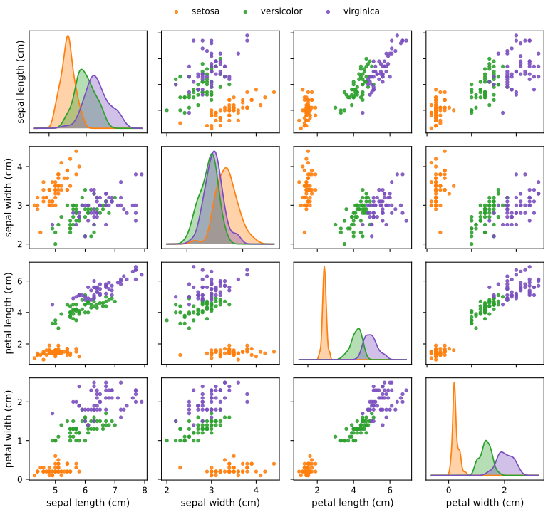
fig_1_3. Reproduces Murphy (2022), Figure 1.3. Download: PDF · SVG1.2.1.3 Learning a classifier
pp. 5–6 Figure 1.3 suggests the rule
\[ f(\mathbf{x};\bm{\theta})=\begin{cases}\text{Setosa}&\text{if petal length}\ \lt\ 2.45\\ \text{Versicolor or Virginica}&\text{otherwise,}\end{cases}\tag{1.1} \]a one-dimensional decision boundary at petal length 2.45 cm. It classifies every Setosa correctly (indeed the two sides separate Setosa from the rest on all 150 flowers), but cannot tell the other two apart. Repeating the idea on the region that failed, with a test on petal width at 1.75 cm, gives a decision tree: internal nodes store a feature and a threshold, and together these are the parameters \(\bm{\theta}\). Figure 1.4 shows the tree and the rectangular regions it defines. (How trees are grown is Section 18.1 of the book; the code here uses the standard greedy search that picks, at each node, the threshold with the smallest weighted Gini impurity.)
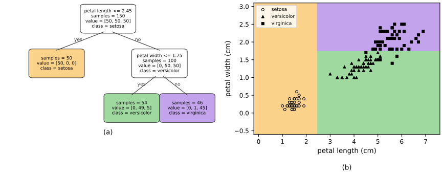
grow_tree, fig_1_4. Reproduces Murphy (2022), Figure 1.4. Download: PDF · SVGSee also (companion course): trees in Elements of Statistical Learning, Section 9.2.3 and Introduction to Statistical Learning, Section 8.1.2.
1.2.1.4 Empirical risk minimization
pp. 6–7 To compare classifiers one needs a number. The simplest is the training misclassification rate
\[ \mathcal{L}(\bm{\theta})\triangleq\frac1N\sum_{n=1}^N\I\big(y_n\neq f(\mathbf{x}_n;\bm{\theta})\big),\tag{1.2} \]where \(\I(e)\) equals 1 if \(e\) is true and 0 otherwise (1.3). It treats all errors alike. If instead some mistakes cost more, we give a loss function \(\ell(y,\hat y)\) and use the empirical risk, the average loss on the training set,
\[ \mathcal{L}(\bm{\theta})\triangleq\frac1N\sum_{n=1}^N\ell\big(y_n,f(\mathbf{x}_n;\bm{\theta})\big).\tag{1.4} \]With the zero-one loss \(\ell_{01}(y,\hat y)=\I(y\neq\hat y)\) (1.5), (1.4) is (1.2). Fitting means choosing the parameters with the smallest empirical risk,
\[ \hat{\bm{\theta}}=\argmin_{\bm{\theta}}\mathcal{L}(\bm{\theta})=\argmin_{\bm{\theta}}\frac1N\sum_{n=1}^N\ell\big(y_n,f(\mathbf{x}_n;\bm{\theta})\big),\tag{1.6} \]which is empirical risk minimization (ERM). The book's running illustration is foraging: Setosa and Versicolor are edible, Virginica is poisonous, so mistaking a Virginica for anything else is much worse than the reverse. Table 1.2 encodes this.
| predicted \(\hat y\) | |||
|---|---|---|---|
| truth \(y\) | Setosa | Versicolor | Virginica |
| Setosa | 0 | 1 | 1 |
| Versicolor | 1 | 0 | 1 |
| Virginica | 10 | 10 | 0 |
Table 1.2 (reproduced). A hypothetical asymmetric loss matrix \(\ell(y,\hat y)\) for Iris classification. Murphy (2022), Table 1.2.
The best classifier for this loss is not the one with the fewest errors, and the next result says exactly what it is. The rows of the matrix are the truth: the loss is 10 when a Virginica is predicted to be Setosa or Versicolor, and 1 for every other mistake.
Result 1.1 (the Bayes decision rule; Table 1.2) pp. 6–7, Section 5.1
Let \((\mathbf{x},y)\) have joint law \(p^*\) and let \(\ell\) be a loss. Among all rules \(\delta:\mathcal{X}\to\mathcal{A}\), the expected loss \(\E\,\ell(y,\delta(\mathbf{x}))\) is smallest for \[ \delta^*(\mathbf{x})\in\argmin_{a}\ \rho(a\given\mathbf{x}),\qquad \rho(a\given\mathbf{x})=\sum_{c=1}^C p^*(y=c\given\mathbf{x})\,\ell(c,a), \] the action of smallest posterior expected loss. For the zero-one loss this is the most probable class. For Table 1.2, writing \(p_1,p_2,p_3\) for the probabilities of Setosa, Versicolor and Virginica, the rule predicts Virginica if \(p_3\ge\max(p_1,p_2)/10\), and otherwise the more probable of Setosa and Versicolor.
Proof
For any rule \(\delta\), conditioning on \(\mathbf{x}\) gives \(\E\,\ell(y,\delta(\mathbf{x}))=\E_{\mathbf{x}}\big[\rho(\delta(\mathbf{x})\given\mathbf{x})\big]\). The integrand is smallest, at every \(\mathbf{x}\) separately, when \(\delta(\mathbf{x})\) minimises \(\rho(\cdot\given\mathbf{x})\), so no rule can have a smaller expectation. (If the minimiser is not unique, any choice works.) For \(\ell_{01}\), \(\rho(a\given\mathbf{x})=1-p^*(a\given\mathbf{x})\), minimised by the largest posterior probability.
For Table 1.2 the three expected losses are \[ \rho(\text{Setosa})=p_2+10p_3,\qquad \rho(\text{Versicolor})=p_1+10p_3,\qquad \rho(\text{Virginica})=p_1+p_2. \] Since \(p_1+p_2=1-p_3\), \(\rho(\text{Virginica})\le\rho(\text{Setosa})\) iff \(p_1\le10p_3\), and \(\rho(\text{Virginica})\le\rho(\text{Versicolor})\) iff \(p_2\le10p_3\). So Virginica is optimal exactly when \(p_3\ge\max(p_1,p_2)/10\). If it fails, Virginica is strictly worse than one of the other two, and between Setosa and Versicolor the difference \(\rho(\text{Setosa})-\rho(\text{Versicolor})=p_2-p_1\) shows Setosa is better iff \(p_1\ge p_2\). ∎
Filling the gap 1.1: the leaves of Figure 1.4 under Table 1.2 pp. 5–7
The book introduces Table 1.2 but never says how it changes the fitted tree. Take the leaf with class counts \((0,49,5)\) of Figure 1.4. Its class proportions are \(p_1=0\), \(p_2=49/54\approx0.907\) and \(p_3=5/54\approx0.093\). Is the majority class still the best prediction?
Derivation
The three expected losses are \(\rho(\text{Setosa})=0.907+0.926=1.833\), \(\rho(\text{Versicolor})=0+0.926=0.926\) and \(\rho(\text{Virginica})=0+0.907=0.907\). The smallest is Virginica, by a hair: indeed \(p_3=0.0926\ge p_2/10=0.0907\). The leaf should therefore predict Virginica although 49 of its 54 flowers are Versicolor. On the 150 training flowers this changes the Table 1.2 empirical risk of the depth-2 tree from \((5\cdot10+1\cdot1)/150=0.340\) (labels by majority class) to \((49\cdot1+1\cdot1)/150=0.333\) (labels by Result 1.1), though the ordinary misclassification rate rises from 4.0% to 33.3%. The two criteria disagree on which tree is best; that is the whole point of specifying a loss. The same computation for the other leaves, \((50,0,0)\) and \((0,1,45)\), leaves their labels unchanged. The demo shows this leaf flipping. ∎
1.2.1.5 Uncertainty
pp. 7–8 A classifier that outputs only a label hides how sure it is, and Result 1.1 shows that the sureness is what the decision needs. There are two reasons we cannot always predict perfectly. Epistemic (model) uncertainty comes from our ignorance of the mapping and can shrink with more data or a better model; aleatoric (data) uncertainty is stochasticity in the world itself and cannot. The probabilistic remedy is to let the model output a distribution over classes,
\[ p(y=c\given\mathbf{x};\bm{\theta})=f_c(\mathbf{x};\bm{\theta}),\tag{1.7} \]with \(f:\mathcal{X}\to[0,1]^C\) and \(\sum_cf_c=1\). To avoid imposing these constraints on \(f\), let it return unconstrained real scores, the logits \(\mathbf{a}=f(\mathbf{x};\bm{\theta})\), and convert them with the softmax
\[ \softmax(\mathbf{a})\triangleq\Big[\frac{e^{a_1}}{\sum_{c'=1}^Ce^{a_{c'}}},\dots,\frac{e^{a_C}}{\sum_{c'=1}^Ce^{a_{c'}}}\Big],\tag{1.8} \] \[ p(y=c\given\mathbf{x};\bm{\theta})=\softmax_c\big(f(\mathbf{x};\bm{\theta})\big).\tag{1.9} \]Filling the gap 1.2: properties of the softmax pp. 7–8, Section 2.5.2
The book asserts that the softmax maps \(\R^C\) into the probability simplex and defers the details. Four facts are used constantly: it is a valid distribution, it ignores a common shift of the logits, its derivative has a closed form, and its negative log is convex.
Derivation
Valid distribution. Each \(e^{a_c}\gt0\), so each coordinate is positive; the coordinates sum to 1 by construction, so each is below 1.
Shift invariance. For any real \(t\), \[ \softmax(\mathbf{a}+t\mathbf{1})_c=\frac{e^{a_c+t}}{\sum_{c'}e^{a_{c'}+t}}=\softmax(\mathbf{a})_c. \] Hence the logits are determined only up to a common constant, and software subtracts \(\max_ca_c\) before exponentiating to avoid overflow. For \(C=2\), \[ \softmax(\mathbf{a})_2=\frac1{1+e^{-(a_2-a_1)}}=\sigma(a_2-a_1), \] the logistic sigmoid of the logit difference.
Derivative. Write \(s_i=\softmax(\mathbf{a})_i\) and \(Z=\sum_ce^{a_c}\). Then \(\partial Z/\partial a_j=e^{a_j}\) and \[ \frac{\partial s_i}{\partial a_j}=\frac{\delta_{ij}e^{a_i}}{Z}-\frac{e^{a_i}e^{a_j}}{Z^2}=s_i(\delta_{ij}-s_j),\qquad\text{i.e. }\ \frac{\partial\mathbf{s}}{\partial\mathbf{a}}=\diag(\mathbf{s})-\mathbf{s}\mathbf{s}^\T. \]
Convexity of the loss. The negative log probability of class \(y\) is \(\lse(\mathbf{a})-a_y\), with \(\lse(\mathbf{a})=\log\sum_ce^{a_c}\). Its gradient is \(\mathbf{s}-\mathbf{e}_y\) and, by the derivative above, the Hessian of \(\lse\) is \(\diag(\mathbf{s})-\mathbf{s}\mathbf{s}^\T\). For any vector \(\mathbf{v}\), \[ \mathbf{v}^\T(\diag(\mathbf{s})-\mathbf{s}\mathbf{s}^\T)\mathbf{v}=\sum_cs_cv_c^2-\Big(\sum_cs_cv_c\Big)^2\ge0, \] the variance of \(v_I\) when the index \(I\) is drawn from \(\mathbf{s}\); so \(\lse\) is convex. Therefore, when \(\mathbf{a}\) is affine in \(\bm{\theta}\) as in (1.10) below, the NLL (1.14) is convex in \(\bm{\theta}\). The variance vanishes for \(\mathbf{v}=\mathbf{1}\), the direction of shift invariance, so the minimiser of the NLL is not unique unless one logit is fixed or a penalty is added. ∎
The simplest logit function is affine,
\[ f(\mathbf{x};\bm{\theta})=b+\mathbf{w}^\T\mathbf{x}=b+w_1x_1+\dots+w_Dx_D,\tag{1.10} \]with \(\bm{\theta}=(b,\mathbf{w})\) (a matrix of weights and a vector of biases when \(C\gt2\)); the model (1.9) with (1.10) is logistic regression, the subject of Chapter 10. Statisticians call \(\mathbf{w}\) the regression coefficients and \(b\) the intercept; the machine learning names are weights and bias. (This "bias" has nothing to do with the statistical bias of an estimator.) To lighten notation one absorbs the bias by setting \(\tilde{\mathbf{w}}=[b,w_1,\dots,w_D]\) and \(\tilde{\mathbf{x}}=[1,x_1,\dots,x_D]\), so that \[ \tilde{\mathbf{w}}^\T\tilde{\mathbf{x}}=b+\mathbf{w}^\T\mathbf{x},\tag{1.11} \] \[ f(\mathbf{x};\mathbf{w})=\mathbf{w}^\T\mathbf{x}\tag{1.12} \] once the tildes are dropped. Because the output is a distribution rather than a label, the smoothed leaf counts in the demo show how even a decision tree can report class probabilities.
See also (companion course): multiclass logistic regression, the Bayes classifier and Bayes rules under different losses.
1.2.1.6 Maximum likelihood estimation
pp. 8–9 When the model outputs probabilities, the natural loss is the negative log probability of the observed output,
\[ \ell\big(y,f(\mathbf{x};\bm{\theta})\big)=-\log p\big(y\given f(\mathbf{x};\bm{\theta})\big),\tag{1.13} \]small when the model gave the true answer high probability (Section 5.1.6.1 of the book explains why this is the right loss). Its average over the training set is the negative log likelihood
\[ \NLL(\bm{\theta})=-\frac1N\sum_{n=1}^N\log p\big(y_n\given f(\mathbf{x}_n;\bm{\theta})\big),\tag{1.14} \]and its minimiser is the maximum likelihood estimate
\[ \hat{\bm{\theta}}_{\rm mle}=\argmin_{\bm{\theta}}\NLL(\bm{\theta}).\tag{1.15} \]Maximising the likelihood \(\prod_np(y_n\given\mathbf{x}_n,\bm{\theta})\) and minimising (1.14) are the same problem, because \(-\frac1N\log\) is a decreasing transformation.
1.2.2 Regression
pp. 8–9 When the output is a real number, \(y\in\R\), the task is regression. Everything above goes through with a different loss. The standard one is the quadratic (\(\ell_2\)) loss \(\ell_2(y,\hat y)=(y-\hat y)^2\) (1.16), which penalises large residuals \(y-\hat y\) heavily (when outliers are present, the absolute loss is more robust; see Section 11.6 of the book). Its empirical risk is the mean squared error
\[ \MSE(\bm{\theta})=\frac1N\sum_{n=1}^N\big(y_n-f(\mathbf{x}_n;\bm{\theta})\big)^2.\tag{1.17} \]To make probabilistic predictions we model the output as Gaussian around the prediction,
\[ \N(y\given\mu,\sigma^2)\triangleq\frac1{\sqrt{2\pi\sigma^2}}\,e^{-\frac1{2\sigma^2}(y-\mu)^2},\tag{1.18} \] \[ p(y_n\given\mathbf{x}_n;\bm{\theta})=\N\big(y_n\given f(\mathbf{x}_n;\bm{\theta}),\sigma^2\big),\tag{1.19} \]where \(\mu=f(\mathbf{x}_n;\bm{\theta})\) is the mean and \(\sigma^2\) the variance (here a fixed constant). The average negative log likelihood is then
\[ \NLL(\bm{\theta})=-\frac1N\sum_{n=1}^N\log\Big[\Big(\frac1{2\pi\sigma^2}\Big)^{1/2}\exp\Big(-\frac1{2\sigma^2}\big(y_n-f(\mathbf{x}_n;\bm{\theta})\big)^2\Big)\Big]\tag{1.20} \] \[ =\frac1{2\sigma^2}\MSE(\bm{\theta})+\const.\tag{1.21} \]Result 1.2 (squared error is Gaussian maximum likelihood) pp. 8–9, (1.17)–(1.21)
For the model (1.19), the NLL equals exactly \(\NLL(\bm{\theta})=\dfrac{1}{2\sigma^2}\MSE(\bm{\theta})+\dfrac12\log(2\pi\sigma^2)\). Consequently (i) for any fixed \(\sigma^2\gt0\) the maximum likelihood estimate of \(\bm{\theta}\) minimises the MSE and does not depend on \(\sigma^2\); and (ii) if \(\sigma^2\) is also estimated, its maximum likelihood estimate at \(\hat{\bm{\theta}}\) is \(\hat\sigma^2=\MSE(\hat{\bm{\theta}})\).
Proof
Take the logarithm inside (1.20), with \(r_n=y_n-f(\mathbf{x}_n;\bm{\theta})\): \[ -\log\big[(2\pi\sigma^2)^{-1/2}e^{-r_n^2/2\sigma^2}\big]=\tfrac12\log(2\pi\sigma^2)+\frac{r_n^2}{2\sigma^2}. \] Averaging over \(n\) gives the stated identity; the "constant" of (1.21) is \(\tfrac12\log(2\pi\sigma^2)\), constant in \(\bm{\theta}\) but not in \(\sigma^2\). (i) The first term is a positive multiple of the MSE, so the minimisers over \(\bm{\theta}\) coincide for every \(\sigma^2\). (ii) Fix \(\bm{\theta}\) and write \(m=\MSE(\bm{\theta})\gt0\) and \(v=\sigma^2\). Then \(g(v)=m/(2v)+\tfrac12\log(2\pi v)\) has \(g'(v)=-m/(2v^2)+1/(2v)\), negative for \(v\lt m\) and positive for \(v\gt m\), so \(g\) is minimised at \(v=m\). ∎
Filling the gap 1.3: why the Gaussian, and what the constant hides p. 9
The book says that minimising the MSE "seems a sensible approach" once it is the Gaussian MLE. Two remarks make this precise. First, the equivalence is a statement about the loss, not a claim that errors are Gaussian: least squares is still the right estimator of a conditional mean when the noise is not Gaussian (its estimand is \(\E[y\given\mathbf{x}]\), see Filling the gap 1.4), but then the stated uncertainty \(\sigma^2\) can be badly calibrated. Second, when the noise has heavier tails, the Gaussian NLL gives large residuals a quadratic penalty and one outlier can dominate the fit; replacing the Gaussian by a Laplace density gives \(\ell_1\) loss in exactly the same way.
Derivation (Laplace noise gives absolute error)
With \(p(y\given\mathbf{x})=\frac1{2b}\exp(-|y-f|/b)\), \(-\log p=\log(2b)+|y-f|/b\), so the NLL is \(\frac1b\cdot\frac1N\sum_n|y_n-f(\mathbf{x}_n)|+\log2b\), a multiple of the mean absolute error plus a constant: the same argument as Result 1.2 with absolute instead of squared residuals. It is the ML counterpart of footnote 4 of the book. ∎
1.2.2.1 Linear regression
pp. 9–10 The simplest regression function is the line \(f(x;\bm{\theta})=b+wx\) (1.22), with slope \(w\), offset \(b\) and parameters \(\bm{\theta}=(w,b)\). Adjusting them to minimise the sum of the squared vertical distances to the points (Figure 1.5b) gives the least squares solution
\[ \hat{\bm{\theta}}=\argmin_{\bm{\theta}}\MSE(\bm{\theta})\tag{1.23} \](computed in Section 11.2.2.1 of the book). With several inputs the model is \(f(\mathbf{x};\bm{\theta})=b+w_1x_1+\dots+w_Dx_D=b+\mathbf{w}^\T\mathbf{x}\) (1.24), multiple linear regression; for temperature as a function of position in a room, \(f(\mathbf{x};\bm{\theta})=b+w_1x_1+w_2x_2\) (1.25).
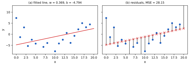
fig_1_5. Reproduces Murphy (2022), Figure 1.5. Download: PDF · SVG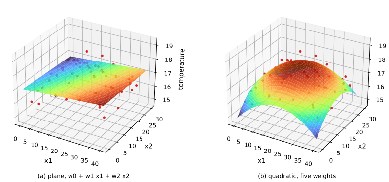
temperature_field, fig_1_6. Reproduces Murphy (2022), Figure 1.6. Download: PDF · SVG1.2.2.2 Polynomial regression
pp. 10–12 The line of Figure 1.5a plainly misses the curvature. A degree-\(D\) polynomial regression model is \(f(x;\mathbf{w})=\mathbf{w}^\T\bphi(x)\) with the feature vector
\[ \bphi(x)=[1,x,x^2,\dots,x^D].\tag{1.26} \]Building \(\bphi\) by hand is feature engineering. The same idea works in several variables: a quadratic expansion of two inputs gives
\[ f(\mathbf{x};\mathbf{w})=w_0+w_1x_1+w_2x_2+w_3x_1^2+w_4x_2^2,\tag{1.27} \]and cross terms such as \(x_1x_2\) capture interactions (see Section 1.5.3.2). The model is still a linear function of the weights even though it is nonlinear in the input, and that is what makes it tractable.
Filling the gap 1.4: least squares, convexity and interpolation pp. 9–12
Three statements are made without proof: the least squares solution exists (1.23), a model linear in its parameters has "a unique global optimum", and a polynomial of degree \(N-1\) fits \(N\) points perfectly. Each needs a hypothesis. Write the model as \(f(\mathbf{x}_n;\mathbf{w})=\bphi(\mathbf{x}_n)^\T\mathbf{w}\) and let \(\bPhi\in\R^{N\times M}\) have rows \(\bphi(\mathbf{x}_n)^\T\), so \(\MSE(\mathbf{w})=\frac1N\|\mathbf{y}-\bPhi\mathbf{w}\|^2\).
Derivation
Normal equations. \(\nabla\MSE=\frac2N\bPhi^\T(\bPhi\mathbf{w}-\mathbf{y})\) and the Hessian is \(\frac2N\bPhi^\T\bPhi\). Setting the gradient to zero gives \(\bPhi^\T\bPhi\mathbf{w}=\bPhi^\T\mathbf{y}\). The system always has a solution, since \(\bPhi^\T\mathbf{y}\in\col(\bPhi^\T)=\col(\bPhi^\T\bPhi)\).
Convexity and uniqueness. For any \(\mathbf{v}\), \(\mathbf{v}^\T\bPhi^\T\bPhi\mathbf{v}=\|\bPhi\mathbf{v}\|^2\ge0\), so the Hessian is positive semi-definite and the MSE is convex: every stationary point is a global minimum. It is strictly convex, hence has a unique minimiser, if and only if \(\bPhi\mathbf{v}=0\Rightarrow\mathbf{v}=0\), that is \(\rank\bPhi=M\) (full column rank). So the book's "unique global optimum" needs the features to be linearly independent on the training inputs. If \(\rank\bPhi\lt M\) the minimisers form an affine subspace \(\hat{\mathbf{w}}+\ker\bPhi\) and all give the same predictions on the training inputs; the one of smallest norm is \(\bPhi^+\mathbf{y}\).
Interpolation. Take \(\bphi(x)=[1,x,\dots,x^{N-1}]\) at \(N\) distinct points \(x_1,\dots,x_N\). If \(\bPhi\mathbf{v}=0\), the polynomial \(\sum_jv_jx^j\) of degree at most \(N-1\) vanishes at \(N\) distinct points, so all its coefficients are zero; \(\bPhi\) is square and invertible (its determinant is \(\prod_{i\lt j}(x_j-x_i)\ne0\)). Hence \(\mathbf{w}=\bPhi^{-1}\mathbf{y}\) gives zero residuals and zero MSE, and it is the unique minimiser. With a repeated input value the targets there must agree for an exact fit. For degree \(D\ge N\) the rank is \(N\lt D+1\) and the minimiser is no longer unique.
The training error never rises with the degree. The polynomials of degree \(D\) are contained in those of degree \(D+1\), so the minimum over the larger set is no larger. This is why training error alone always prefers the most flexible model (Section 1.2.3). ∎
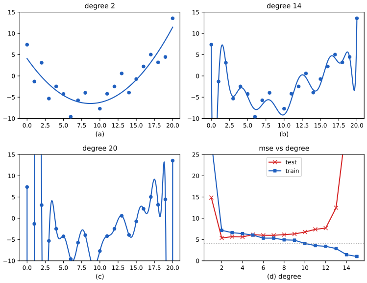
poly_fit, fig_1_7. Reproduces Murphy (2022), Figure 1.7. Download: PDF · SVGSee also (companion course): polynomial curve fitting with the same phenomenon, linear regression with basis functions and the curve fitting demo.
1.2.2.3 Deep neural networks
p. 12 Polynomial features are chosen by hand. A far more flexible model lets the feature extractor have its own parameters \(\mathbf{V}\) and learns them too:
\[ f(\mathbf{x};\mathbf{w},\mathbf{V})=\mathbf{w}^\T\bphi(\mathbf{x};\mathbf{V}).\tag{1.28} \]Decomposing \(\bphi\) recursively into simple functions gives a stack of \(L\) nested layers,
\[ f(\mathbf{x};\bm{\theta})=f_L\big(f_{L-1}(\cdots(f_1(\mathbf{x}))\cdots)\big),\tag{1.29} \]with \(f_\ell(\mathbf{x})=f(\mathbf{x};\bm{\theta}_\ell)\) the \(\ell\)th layer. The last layer is linear, \(f_L(\mathbf{x})=\mathbf{w}_L^\T\mathbf{x}\), so the first \(L-1\) layers form a learned feature extractor. This is a deep neural network (DNN); convolutional networks (CNNs) are the variant for images and recurrent networks (RNNs) the variant for sequences (Part III of the book). Unlike the polynomial, the model is not linear in \(\bm{\theta}\), so the loss need not be convex.
See also (companion courses): Bayesian and Probabilistic Machine Learning, Chapter 5 and the Foundations of Deep Learning course.
1.2.3 Overfitting and generalization
pp. 12–13 The empirical risk can be written so as to name the data set it is computed on,
\[ \mathcal{L}(\bm{\theta};\mathcal{D}_{\rm train})=\frac1{|\mathcal{D}_{\rm train}|}\sum_{(\mathbf{x},y)\in\mathcal{D}_{\rm train}}\ell\big(y,f(\mathbf{x};\bm{\theta})\big).\tag{1.30} \]A flexible enough model can make this zero by memorising (Figure 1.7c), but what we care about is performance on new data. If the data-generating distribution \(p^*(\mathbf{x},y)\) were known we would measure the population risk
\[ \mathcal{L}(\bm{\theta};p^*)\triangleq\E_{p^*(\mathbf{x},y)}\big[\ell(y,f(\mathbf{x};\bm{\theta}))\big];\tag{1.31} \]the difference \(\mathcal{L}(\bm{\theta};p^*)-\mathcal{L}(\bm{\theta};\mathcal{D}_{\rm train})\) is the generalization gap, and a large gap signals overfitting. Since \(p^*\) is unknown, one holds out a test set and estimates (1.31) by the test risk
\[ \mathcal{L}(\bm{\theta};\mathcal{D}_{\rm test})\triangleq\frac1{|\mathcal{D}_{\rm test}|}\sum_{(\mathbf{x},y)\in\mathcal{D}_{\rm test}}\ell\big(y,f(\mathbf{x};\bm{\theta})\big).\tag{1.32} \]In Figure 1.7d the training error goes to zero as the degree grows, while the test error is U-shaped: at degree 1 the model underfits, at high degree it overfits, and degree 2 is "just right". Choosing among models by their training loss always favours the largest. The book's remedy is a three-way split: a training set to fit, a validation set to choose the model, and a test set that is touched only once to report the final performance (Section 4.5.4).
A remark on the book
The text says one should "pick the model with minimum test loss", and then, one sentence later, introduces the validation set precisely because choosing on the test set contaminates it. The correct reading is the second: models are chosen by validation (or cross-validation) loss. The first sentence is a shorthand about held-out data, not a recommendation to tune on the final test set. Using the test set for selection biases its risk estimate downward, because the winning model was chosen for doing well on exactly those points.
Result 1.3 (the optimism of the training error) Section 1.2.3, Figure 1.7d
Fix \(N\) input points, let \(\mathbf{y}=\mathbf{f}+\bm{\varepsilon}\) with \(\E\bm{\varepsilon}=0\), \(\cov\bm{\varepsilon}=\sigma^2\mathbf{I}\), and let \(\mathbf{y}'=\mathbf{f}+\bm{\varepsilon}'\) be a fresh copy of the noise at the same inputs. Fit least squares with a model of \(p\) linearly independent features, \(\hat{\mathbf{y}}=\mathbf{H}\mathbf{y}\) where \(\mathbf{H}\) is the projection onto the column space of the design matrix. Then, with \(\MSE_{\rm train}=\frac1N\|\mathbf{y}-\hat{\mathbf{y}}\|^2\) and \(\MSE_{\rm test}=\frac1N\|\mathbf{y}'-\hat{\mathbf{y}}\|^2\), \[ \E\,\MSE_{\rm train}=\frac1N\|(\mathbf{I}-\mathbf{H})\mathbf{f}\|^2+\sigma^2\Big(1-\frac pN\Big),\qquad \E\,\MSE_{\rm test}=\frac1N\|(\mathbf{I}-\mathbf{H})\mathbf{f}\|^2+\sigma^2\Big(1+\frac pN\Big), \] so the expected generalization gap is exactly \(2\sigma^2p/N\), whatever the true \(\mathbf{f}\) (the model may be wrong).
Filling the gap 1.5: proof of Result 1.3 and what Figure 1.7d does differently p. 13
The book describes the U-shaped test curve in words. Result 1.3 quantifies it in the cleanest setting (a fixed design) and explains why the training curve of a degree-\((N-1)\) polynomial must reach zero: with \(p=N\) the gap is \(2\sigma^2\) and the training error is \(\sigma^2(1-p/N)=0\) when the model is exact.
Proof
\(\mathbf{H}\) is symmetric and idempotent with trace \(p\) (the trace of a projection is its rank). Write \(\mathbf{r}=(\mathbf{I}-\mathbf{H})\mathbf{y}=(\mathbf{I}-\mathbf{H})\mathbf{f}+(\mathbf{I}-\mathbf{H})\bm{\varepsilon}\). Then \[ \|\mathbf{r}\|^2=\|(\mathbf{I}-\mathbf{H})\mathbf{f}\|^2+2\mathbf{f}^\T(\mathbf{I}-\mathbf{H})\bm{\varepsilon}+\bm{\varepsilon}^\T(\mathbf{I}-\mathbf{H})\bm{\varepsilon}. \] The cross term has mean zero, and \[ \E\,\bm{\varepsilon}^\T(\mathbf{I}-\mathbf{H})\bm{\varepsilon}=\sigma^2\Tr(\mathbf{I}-\mathbf{H})=\sigma^2(N-p). \] Dividing by \(N\) gives the first formula.
For the test error, \(\mathbf{y}'-\hat{\mathbf{y}}=\bm{\varepsilon}'+(\mathbf{f}-\hat{\mathbf{y}})\) with \(\bm{\varepsilon}'\) independent of \(\hat{\mathbf{y}}\), so \[ \E\|\mathbf{y}'-\hat{\mathbf{y}}\|^2=N\sigma^2+\E\|\mathbf{f}-\mathbf{H}\mathbf{f}-\mathbf{H}\bm{\varepsilon}\|^2=N\sigma^2+\|(\mathbf{I}-\mathbf{H})\mathbf{f}\|^2+\sigma^2p, \] again with a vanishing cross term because \((\mathbf{I}-\mathbf{H})\mathbf{f}\perp\mathbf{H}\bm{\varepsilon}\). Subtracting the two expectations gives \(\sigma^2(N+p)-\sigma^2(N-p)=2\sigma^2p\), divided by \(N\). ∎
What changes in Figure 1.7d. There the test points have new inputs as well as new noise, so the gap is larger than \(2\sigma^2p/N\) and grows sharply when the polynomial oscillates between and beyond the training points (the variance of \(\hat f\) at an input far from the data is large). The fixed-design formula gives the lower bound for that effect. Figure 1.S2 below checks it by simulation.
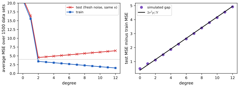
optimism_experiment, fig_1_S2. Download: PDF · SVGSee also (companion course): Section 7.4 of the Elements of Statistical Learning course derives the optimism for general losses and links it to AIC and \(C_p\); Bayesian and Probabilistic Machine Learning, Section 3.2 gives the bias–variance decomposition.
1.2.4 No free lunch theorem
p. 13 With so many models, one asks which is best. The no free lunch theorem (Wolpert, 1996) says that none is best for every problem: whatever assumptions about the world a model builds in (its inductive bias) help where they hold and hurt where they do not. So the choice rests on domain knowledge or on trial and error with model selection (cross validation, Section 4.5.4; Bayesian methods, Sections 5.2.2 and 5.2.6), and it pays to know many methods.
Result 1.4 (a finite no free lunch statement) p. 13; Wolpert (1996)
Let \(\mathcal{X}\) be a finite set, let a learner see the labels of a training set \(S\subset\mathcal{X}\) and then predict a label for every point of \(\mathcal{X}\setminus S\) (any deterministic or randomised learner). Draw the true labelling \(f:\mathcal{X}\to\{0,1\}\) uniformly from all \(2^{|\mathcal{X}|}\) labellings. Then the expected error on \(\mathcal{X}\setminus S\) is exactly \(1/2\), for every learner.
Filling the gap 1.6: proof, and what the theorem does not say p. 13
The book states the theorem in words. Here is a proof and a reading of the result.
Proof and interpretation
Fix the training inputs \(S\) and any learner. Under the uniform law, the labels \(f(x)\), \(x\in\mathcal{X}\), are independent fair coins. The learner's prediction \(\hat f(x)\) for \(x\notin S\) is a function of \(S\), the training labels and possibly internal randomness; none of these involves \(f(x)\), so \(\hat f(x)\) is independent of \(f(x)\), which is a fair coin. Hence \(\Pr(\hat f(x)\ne f(x))=\tfrac12\) for each \(x\notin S\), and the expected error on \(\mathcal{X}\setminus S\) is \(\tfrac12\). ∎
I confirmed this by enumerating all \(2^8\) labellings of an 8-point domain with three training points for four learners (majority vote, nearest neighbour, always predict 1, and the contrarian anti-nearest-neighbour): all four average exactly \(1/2\). Reading. The uniform average over problems is a statement that without assumptions, labels at unseen points carry no information from seen points. Real problems are not uniform: they have structure (smoothness, sparsity, invariance) and inductive biases are bets on that structure. The theorem says the bet must be matched to the problem; it does not say learning is impossible. Equivalently, "learning works" means the true \(f\) has high prior probability under the learner's assumptions.
See also (companion course): model selection and error rates and the Bayes classifier.
1.3 Unsupervised learning
p. 14 In unsupervised learning we get inputs \(\mathcal{D}=\{\mathbf{x}_n\}_{n=1}^N\) and no outputs, and try to "make sense" of them. Probabilistically, supervised learning fits a conditional model \(p(y\given\mathbf{x})\), while unsupervised learning fits an unconditional one, \(p(\mathbf{x})\), which can also generate new data. (Statisticians write \(x\) for the exogenous variables that are not modelled, so for them the unconditional model would be \(p(y)\).) Three reasons make it attractive. No labels need be collected, which is slow and costly. It avoids imposing arbitrary categories: whether a person is "drinking" or "sipping" is hard to define, and annotators disagree, so a learner should not be expected to reproduce one fixed labelling (a more reasonable target is the distribution of labels a crowd would give). And it forces the model to explain the whole high-dimensional input rather than a few output bits, which is the point of Hinton's rough arithmetic: a brain has some \(10^{14}\) connections and lives about \(10^9\) seconds, so it must absorb about \(10^5\) bits per second, far more than any teacher supplies.
1.3.1 Clustering
pp. 14–15 The simplest task is to partition the inputs into groups of similar points. In the two petal features of Iris with the labels hidden, there are plainly two blobs, and if good clusters are compact one may split the upper blob again, giving three (Figure 1.8). There is no "correct" number of clusters; one trades model complexity against fit (Section 21.3.7). The code uses Lloyd's algorithm for K-means, which alternates between assigning each point to the nearest centre and moving each centre to the mean of its points.
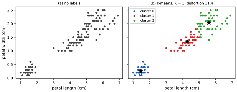
kmeans, fig_1_8. Reproduces Murphy (2022), Figure 1.8. Download: PDF · SVGFilling the gap 1.7: Lloyd's algorithm decreases the distortion at every step pp. 14–15
The book describes the clusters but not why the procedure behind them works. Define the distortion for assignments \(z_n\in\{1,\dots,K\}\) and centres \(\bm{\mu}_1,\dots,\bm{\mu}_K\) by \(J(\mathbf{z},\bm{\mu})=\sum_{n}\|\mathbf{x}_n-\bm{\mu}_{z_n}\|^2\).
Derivation
Assignment step. For fixed \(\bm{\mu}\), \(J\) is a sum over \(n\) of terms that each depend only on \(z_n\), so it is minimised by sending every point to its nearest centre. Update step. For fixed \(\mathbf{z}\), \(J\) separates over clusters, and for a cluster \(S\) with mean \(\bar{\mathbf{x}}\) and any centre \(\mathbf{m}\), \[ \sum_{n\in S}\|\mathbf{x}_n-\mathbf{m}\|^2=\sum_{n\in S}\|\mathbf{x}_n-\bar{\mathbf{x}}\|^2+|S|\,\|\mathbf{m}-\bar{\mathbf{x}}\|^2 \] (the cross term is \(2(\bar{\mathbf{x}}-\mathbf{m})^\T\sum_{n\in S}(\mathbf{x}_n-\bar{\mathbf{x}})=0\)), which is smallest at \(\mathbf{m}=\bar{\mathbf{x}}\). Each of the two steps therefore leaves \(J\) unchanged or lowers it. \(J\ge0\) and there are only \(K^N\) assignments, so the sequence of distortions converges and the algorithm stops after finitely many steps (it stops when the assignments no longer change). It reaches a local minimum, not necessarily the global one, which is why several random starts are used. Taking \(K=N\) gives \(J=0\): the distortion alone cannot choose \(K\). ∎
See also (companion course): K-means in Chapter 9 (as a limit of a Gaussian mixture), Section 12.4.1 of Introduction to Statistical Learning and the K-means and EM demo.
1.3.2 Discovering latent "factors of variation"
pp. 15–16 For high-dimensional data one hopes that each observation \(\mathbf{x}_n\in\R^D\) was produced by a few hidden factors \(\mathbf{z}_n\in\R^K\), \(K\ll D\) (the arrow \(\mathbf{z}_n\to\mathbf{x}_n\) stands for "causes"). Since the \(\mathbf{z}_n\) are unobserved we give them a simple prior, typically Gaussian, and for real-valued data a Gaussian likelihood too. The simplest case is linear,
\[ p(\mathbf{x}_n\given\mathbf{z}_n;\bm{\theta})=\N(\mathbf{x}_n\given\mathbf{W}\mathbf{z}_n+\bm{\mu},\bm{\Sigma}),\]which is factor analysis; with \(\bm{\Sigma}=\sigma^2\mathbf{I}\) it is probabilistic PCA (Section 20.1). It looks like linear regression with the inputs \(\mathbf{z}_n\) never observed. Figure 1.9 fits a two-dimensional plane to three Iris features. Replacing the linear map by a neural network \(f(\mathbf{z};\bm{\theta})\) gives nonlinear models, much harder to fit because the network inputs must be inferred as well; the variational autoencoder (Section 20.3.5) is one approximate method.
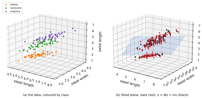
pca, fig_1_9. Reproduces Murphy (2022), Figure 1.9. Download: PDF · SVGFilling the gap 1.8: the marginal of factor analysis, and why PCA fits the best plane pp. 15–16, Section 20.1
Two facts underlie Figure 1.9 and are not shown: the observed-data distribution implied by the latent model, and the optimality of the plane found from the SVD. Assume \(\mathbf{z}\sim\N(\mathbf{0},\mathbf{I}_K)\) and \(\mathbf{x}=\mathbf{W}\mathbf{z}+\bm{\mu}+\bm{\varepsilon}\), \(\bm{\varepsilon}\sim\N(\mathbf{0},\bm{\Sigma})\) independent of \(\mathbf{z}\).
Derivation
Marginal. \(\mathbf{x}\) is an affine function of the jointly Gaussian pair \((\mathbf{z},\bm{\varepsilon})\), hence Gaussian, with mean \(\bm{\mu}\) and covariance \(\E[(\mathbf{W}\mathbf{z}+\bm{\varepsilon})(\mathbf{W}\mathbf{z}+\bm{\varepsilon})^\T]=\mathbf{W}\mathbf{W}^\T+\bm{\Sigma}\) (the cross terms vanish by independence). So \(p(\mathbf{x})=\N(\bm{\mu},\mathbf{W}\mathbf{W}^\T+\bm{\Sigma})\): a Gaussian with a low-rank-plus-diagonal covariance. Replacing \(\mathbf{W}\) by \(\mathbf{W}\mathbf{R}\) with \(\mathbf{R}\) orthogonal leaves it unchanged, so the latent axes are not identifiable, only the plane they span.
Best plane. Let \(\mathbf{S}=\frac1N\sum_n(\mathbf{x}_n-\bar{\mathbf{x}})(\mathbf{x}_n-\bar{\mathbf{x}})^\T\) have eigenpairs \((\lambda_i,\mathbf{u}_i)\), \(\lambda_1\ge\dots\ge\lambda_D\). Among all orthonormal \(\mathbf{W}\in\R^{D\times K}\), the squared reconstruction error of projecting the centred data is \(\sum_n\|\mathbf{x}_n-\bar{\mathbf{x}}\|^2-N\Tr(\mathbf{W}^\T\mathbf{S}\mathbf{W})\), so minimising the error is maximising \(\Tr(\mathbf{W}^\T\mathbf{S}\mathbf{W})=\sum_i\lambda_iq_i\) with \(q_i=\|\mathbf{W}^\T\mathbf{u}_i\|^2\). Each \(q_i\in[0,1]\) (a projection cannot lengthen a unit vector) and \(\sum_iq_i=\|\mathbf{W}\|_F^2=K\); a linear function over this set is maximised by putting all the weight on the largest eigenvalues, \(q_1=\dots=q_K=1\), i.e. \(\mathbf{W}=[\mathbf{u}_1,\dots,\mathbf{u}_K]\) up to rotation. The error is then \(N\sum_{i\gt K}\lambda_i=\sum_{i\gt K}s_i^2\), where \(s_i=\sqrt{N\lambda_i}\) are the singular values of the centred data matrix. The probabilistic PCA likelihood has the same maximiser for \(\mathbf{W}\) (Tipping and Bishop, 1999), with \(\hat\sigma^2\) the average of the discarded eigenvalues. ∎
See also (companion course): the minimum-error formulation of PCA, probabilistic PCA, Section 12.2 of Introduction to Statistical Learning and the PCA demo.
1.3.3 Self-supervised learning
p. 16 In self-supervised learning one manufactures a supervised problem out of unlabelled data: predict the colours of an image from its greyscale version, or hide words in a sentence and predict them from their neighbours. In the notation of the book, a predictor \(\hat{\mathbf{x}}_1=f(\mathbf{x}_2;\bm{\theta})\) of one part of the input from another part is trained for its own sake, and the features it learns are reused for downstream supervised tasks. The appeal is that it needs only standard supervised machinery and sidesteps inferring the true latent factors (Section 19.2).
1.3.4 Evaluating unsupervised learning
pp. 16–17 With no ground truth, unsupervised methods are hard to score. A common criterion is the probability the model gives to unseen examples, i.e. the average negative log likelihood
\[ \mathcal{L}(\bm{\theta};\mathcal{D})=-\frac1{|\mathcal{D}|}\sum_{\mathbf{x}\in\mathcal{D}}\log p(\mathbf{x}\given\bm{\theta}),\tag{1.33} \]which treats the task as density estimation: probabilities sum to one, so a model that puts mass where the data lie must put little elsewhere. This is also what a compressor needs. Density estimation is hard in high dimension, and a model with high likelihood may still have missed high-level structure (the extreme case is memorising the training examples). Alternatives: use the learned representation as the input of a supervised learner and count how few labelled examples then suffice (sample efficiency), or, in science, judge the model by how well it explains and can be interpreted, which usually requires experiments.
Filling the gap 1.9: the average NLL is a KL divergence plus an entropy p. 16, (1.33)
The book says that fitting \(p(\mathbf{x}\given\bm{\theta})\) by (1.33) captures "the typical patterns in the data". The precise statement: let \(p^*\) be the true density and \(q_{\bm{\theta}}=p(\cdot\given\bm{\theta})\). For a large test set, (1.33) converges to \(\E_{p^*}[-\log q_{\bm{\theta}}]=H(p^*)+\KL(p^*\,\|\,q_{\bm{\theta}})\), where \(H(p^*)=-\E_{p^*}\log p^*\) is the entropy and \(\KL(p\|q)=\E_p\log(p/q)\). So NLL is minimised by the model closest to the truth in KL, and its minimum value is \(H(p^*)\), reached only when \(q_{\bm{\theta}}=p^*\).
Derivation
\(-\log q=-\log p^*+\log(p^*/q)\); take \(\E_{p^*}\). \(\KL\ge0\) with equality iff \(p=q\) almost everywhere: by Jensen's inequality for the strictly concave logarithm, \[ -\KL(p\|q)=\E_p\log\frac qp\le\log\E_p\frac qp=\log\int_{p\gt0}q\le\log1=0, \] with equality iff \(q/p\) is constant on \(\{p\gt0\}\) and \(q\) has no mass outside. Likewise, with the empirical distribution \(\hat p\) of the training data (a sum of point masses), (1.33) \(=H(\hat p,q_{\bm{\theta}})\) and the MLE is the \(q_{\bm{\theta}}\) closest to \(\hat p\) in the sense that it minimises \(\KL(\hat p\|q_{\bm{\theta}})\) up to the constant \(H(\hat p)\). One caution for continuous \(\mathbf{x}\): densities are not bounded by 1, and a flexible model can drive the training NLL to \(-\infty\) (a Gaussian mixture with one component shrunk onto a single point), which is the memorisation the book warns of; hold-out NLL is what has meaning. ∎
See also (companion course): relative entropy and mutual information in Chapter 1 of Bayesian and Probabilistic Machine Learning.
1.4 Reinforcement learning
pp. 17–18 In reinforcement learning (RL) a system, the agent, interacts with an environment and must learn a policy \(a=\pi(\mathbf{x})\) that maps what it observes to an action. A game-playing agent sees the image and chooses a move; a walking robot sees its joint angles and chooses motor signals (Figure 1.10, two screenshots, not reproduced). Unlike supervised learning, nobody says which action was right: there is only an occasional reward or penalty, like a critic's thumbs up or down rather than a teacher's instruction. The difficulty is that the reward is sparse and delayed (a chess game gives a single win or loss at its end), so credit for it must be assigned to the many actions that came before. To compensate one uses other information: demonstrations from an expert, which supervised learning can digest, and unlabelled data from which an unsupervised model can learn how the environment behaves. LeCun's picture (Figure 1.11, a diagram, not reproduced) makes unsupervised learning the cake, supervised learning the icing and RL the cherry, the claim being that most of the information must come from unsupervised learning. Reinforcement learning is treated in the sequel to the book (Murphy, 2023).
See also (companion course): decision-making under a loss in Result 1.1 is the one-step case of RL (a policy that minimises expected loss, here with no later consequences).
1.5 Data
p. 19 Machine learning fits models to data with algorithms, and the nature and quality of the data matter as much as either. This section lists the data sets used in the book and some standard preprocessing.
1.5.1 Some common image datasets
1.5.1.1 Small image datasets
pp. 19–20 MNIST (LeCun et al., 1998) has 60,000 training and 10,000 test greyscale images of handwritten digits, each \(28\times28\) with integer pixel values 0 to 255 (usually rescaled to \([0,1]\) or thresholded to binary). The images were preprocessed to centre the digits, hence "modified" in the name. Hinton called it the "drosophila of machine learning", a model organism on which a method must work before it can hope to work on harder data. By modern standards it is easy, and the book remarks that most pairs of digits can be told apart from a single pixel. I checked that claim on 20,000 training images: for each of the 45 pairs of digits I found the best single pixel (thresholded at 0.5) and used it as a classifier. The median pair is separated with 84% accuracy, 82% of the pairs with more than 80%, but only 16% of the pairs with more than 90%; so the remark holds in the sense of "much better than chance", not of "nearly perfectly".
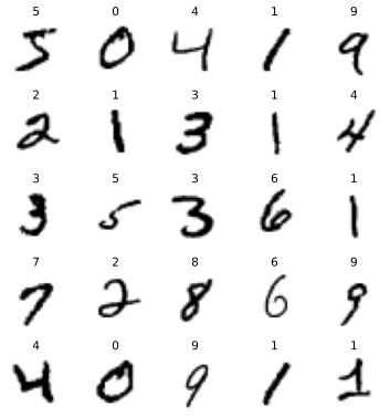
fig_1_12. Reproduces Murphy (2022), Figure 1.12(a). Download: PDF · SVGVariants address MNIST's easiness. EMNIST (Cohen et al., 2017) adds lower- and upper-case letters, giving 62 classes some of which are ambiguous (the digit 1 and the letter l). Fashion-MNIST (Xiao et al., 2017) has the same size and format but shows ten kinds of clothing (Figure 1.13a, a sample of images, not reproduced). For small colour images the standard is CIFAR (Krizhevsky and Hinton, 2009): 60,000 images of \(32\times32\times3\) in 10 or 100 classes (Figure 1.13b, not reproduced). The data sets have flaws: a share of the CIFAR-100 labels are wrong, which puts a ceiling below 100% on achievable accuracy, and some training images reappear in the test set (cited in the book as Northcutt et al., 2021, and Barz and Denzler, 2020).
1.5.1.2 ImageNet
pp. 20–21 Small data sets are for prototyping; ImageNet (Russakovsky et al., 2015) has about 14 million images in some 20,000 classes. Its challenge (ILSVRC, 2010 to 2018) used 1.3 million training images of 1000 classes, scored by top-5 error (is the correct label among the five most probable?). Error fell steadily over the years (Figure 1.14, which shows sample predictions and a history of error rates taken from other sources, not reproduced). In 2015 convolutional networks first outperformed a human labeller on it. This does not mean they see better: the data set contains fine distinctions (a tiger against a tiger cat) that people find hard, and flexible networks can memorise even random labels (Zhang et al., 2017). The benchmark is nearly saturated, yet relative performance on it still predicts performance on unrelated image tasks, which keeps it in use.
1.5.2 Some common text datasets
pp. 21–23 Machine learning applied to text is natural language processing (NLP). Text classification assigns a document a label: spam or not, or the sentiment of a review. The standard benchmark is the IMDB movie review set (Maas et al., 2011): 25,000 labelled reviews for training and 25,000 for testing with a positive or negative label (Table 1.3 in the book shows two snippets, not reproduced). Machine translation maps a sentence to a sentence in another language and needs aligned pairs, available from parliamentary proceedings (Canadian English–French, the European Parliament) and from the WMT English–German set. Seq2seq models, a generalisation to any sequence-to-sequence mapping, handle summarisation or question answering; one casts the latter as: input = passage plus question, output = answer, which is often a stretch of the passage (Table 1.4 and the SQuAD data of Rajpurkar et al., 2016). Language modelling is the unconditional generative modelling of text, \(p(x_1,\dots,x_T)\); it needs only sentences, so it is unsupervised, and becomes conditional (a seq2seq model) when it responds to an input.
1.5.3 Preprocessing discrete input data
p. 23 Many models want real vectors, but inputs can be categories or words.
1.5.3.1 One-hot encoding
A categorical variable \(x\) with \(K\) values is encoded by the one-hot (dummy) vector \(\text{one-hot}(x)=[\I(x=1),\dots,\I(x=K)]\): with colours red, green, blue the codes are \([1,0,0]\), \([0,1,0]\), \([0,0,1]\). Then weighted sums of inputs make sense, since the numerical value no longer encodes a fake ordering.
1.5.3.2 Feature crosses
pp. 23–24 A linear model on one-hot codes captures only main effects: each variable adds its own contribution irrespective of the others. Suppose fuel efficiency depends on vehicle type (SUV, truck, family car) and country of origin (USA, Japan). The concatenated encoding is
\[ \bphi(\mathbf{x})=[1,\ \I(x_1=S),\ \I(x_1=T),\ \I(x_1=F),\ \I(x_2=U),\ \I(x_2=J)],\tag{1.34} \]and cannot say that trucks are worse when made in the USA than in Japan, because the effect of the country is the same for every type. A feature cross introduces one indicator for each of the \(3\times2\) combinations. The model is \(f(\mathbf{x};\mathbf{w})=\mathbf{w}^\T\bphi(\mathbf{x})\) (1.35) with
\[ \begin{aligned}f(\mathbf{x};\mathbf{w})&=w_0+w_1\I(x_1=S)+w_2\I(x_1=T)+w_3\I(x_1=F)+w_4\I(x_2=U)+w_5\I(x_2=J)\\&\quad+w_6\I(x_1=S,x_2=U)+w_7\I(x_1=T,x_2=U)+w_8\I(x_1=F,x_2=U)\\&\quad+w_9\I(x_1=S,x_2=J)+w_{10}\I(x_1=T,x_2=J)+w_{11}\I(x_1=F,x_2=J),\end{aligned}\tag{1.36} \]which turns the table into a wider one with many more columns.
Filling the gap 1.10: how many things can (1.34) and (1.36) represent? pp. 23–24
The book says the main-effects model cannot capture the interaction and the crossed model can. Count the parameters that actually matter. There are six (type, country) cells, so a prediction rule is a vector in \(\R^6\); how much of \(\R^6\) does each design reach? Let \(\mathbf{M}\) and \(\mathbf{M}_\times\) be the \(6\times6\) and \(6\times12\) matrices whose rows are (1.34) and (1.36) at the six cells.
Derivation
Main effects: rank 4. The three type indicators sum to the constant 1, and so do the two country indicators, so the columns of \(\mathbf{M}\) satisfy \(\mathbf{1}=\sum_t\mathbf{c}_t=\sum_c\mathbf{c}_c\). These are two independent linear relations among the six columns, so at most four columns are independent; the constant, two of the type indicators and one country indicator are, and \(\rank\mathbf{M}=1+2+1=4\lt6\). The set of cell-values it can produce is \(\{a_{\rm type}+b_{\rm country}\}\), additive tables: a \(3\times2\) table with \(a+b\) form, which is a 4-dimensional subspace. A table with a nonzero "interaction" \(f(T,U)-f(T,J)-f(F,U)+f(F,J)\neq0\) is outside it. Crossed: rank 6. The six cross indicators \(\I(x_1=t,x_2=c)\) are the standard basis of \(\R^6\) over the cells, so \(\rank\mathbf{M}_\times=6\): every table of cell values can be represented, and the 12 weights are over-parameterised by 6 (the main-effect columns are sums of cross columns). One may thus drop the main effects or keep them with a penalty or constraints. ∎
Numerically, for a vector of cell means \((20,25,12,18,30,31)\) the best main-effects fit leaves a residual of norm greater than 1, while the crossed model reproduces all six cells exactly.
1.5.4 Preprocessing text data
p. 24 Text breaks the assumptions of fixed-length vector models in three ways: documents have different lengths; words are categorical variables with huge vocabularies, whose one-hot vectors carry no notion of similarity; and new words appear at test time (out-of-vocabulary, OOV).
1.5.4.1 Bag of words model
pp. 24–25 A bag of words discards word order. After mapping words to tokens from a vocabulary (usually after dropping punctuation, lower-casing, removing very common stop words such as "and" and "the", and stemming "running" and "runs" to "run"), the \(n\)th document of length \(T\) becomes the count vector \(\tilde{\mathbf{x}}_n\in\R^D\) over the \(D\) vocabulary terms,
\[ \tilde x_{nv}=\sum_{t=1}^T\I(x_{nt}=v),\tag{1.37} \]the vector space model of text. Stacking the \(\tilde{\mathbf{x}}_n\) as rows gives an \(N\times D\) design matrix; in information retrieval one stores the transpose, a \(D\times N\) term-frequency matrix with \(\text{TF}_{ij}\) the count of term \(i\) in document \(j\).
1.5.4.2 TF-IDF
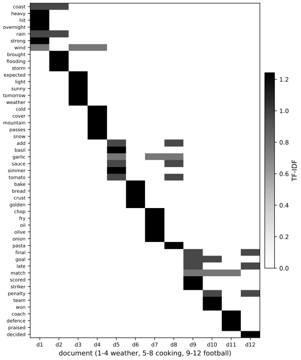
pp. 25 Raw counts overweight words that are frequent but uninformative. Taking logs tames big counts inside a document; to tame words that are common across documents, define the inverse document frequency \(\text{IDF}_i\triangleq\log\frac N{1+\text{DF}_i}\), where \(\text{DF}_i\) is the number of documents containing term \(i\). The TF-IDF matrix is
\[ \text{TFIDF}_{ij}=\log(\text{TF}_{ij}+1)\times\text{IDF}_i\tag{1.38} \](rows are often normalised afterwards). Figure 1.15 shows such a matrix; the code builds it for a small corpus of twelve sentences written for this course (four about weather, four about cooking, four about football), after removing a short list of stop words.
tfidf, fig_1_15. Reproduces Murphy (2022), Figure 1.15. Download: PDF · SVG1.5.4.3 Word embeddings
pp. 25–26 TF-IDF does not cure the root problem of one-hot codes: "man" and "woman" end up no closer than "man" and "banana", so the assumption behind most predictors, that nearby inputs give similar outputs, fails. Word embeddings map each sparse one-hot vector \(\mathbf{x}_{nt}\in\{0,1\}^V\) to a dense vector \(\mathbf{e}_{nt}=\mathbf{E}\mathbf{x}_{nt}\in\R^K\) with a learned matrix \(\mathbf{E}\in\R^{K\times V}\) that places similar words close together (ways to learn \(\mathbf{E}\) are in Section 20.5). A document is then summarised by the sum (or average) of its word embeddings,
\[ \mathbf{e}_n=\sum_{t=1}^T\mathbf{e}_{nt}=\mathbf{E}\tilde{\mathbf{x}}_n,\tag{1.39} \]and fed to a softmax classifier,
\[ p(y=c\given\mathbf{x}_n,\bm{\theta})=\softmax_c\big(\mathbf{W}\mathbf{E}\tilde{\mathbf{x}}_n\big).\tag{1.40} \]With a pretrained \(\mathbf{E}\) the model is linear in \(\mathbf{W}\) (Chapter 10); contextual embeddings are in Section 15.7.
Filling the gap 1.11: the algebra of one-hot codes, TF-IDF and embeddings pp. 24–26
Four small facts back the claims of this subsection.
Derivation
One-hot codes are all equally far apart. For distinct words \(u\ne v\), \(\|\mathbf{e}_u-\mathbf{e}_v\|^2=1+1=2\) and \(\mathbf{e}_u^\T\mathbf{e}_v=0\). So Euclidean distance is \(\sqrt2\) and cosine similarity 0 for every pair: "man" and "banana" look exactly as different as "man" and "woman", which is the book's complaint.
The embedding identity (1.39). A one-hot vector picks out a column: \(\mathbf{E}\mathbf{e}_v=\mathbf{E}_{:,v}\). Therefore \(\sum_t\mathbf{E}\mathbf{x}_{nt}=\mathbf{E}\sum_t\mathbf{x}_{nt}=\mathbf{E}\tilde{\mathbf{x}}_n\), because \(\sum_t\mathbf{x}_{nt}\) is the count vector (1.37): the order of summation and the linear map commute. Then (1.40) is a softmax regression (the model (1.9)) on the \(K\)-dimensional features \(\mathbf{E}\tilde{\mathbf{x}}_n\), and as a function of the raw counts it is a softmax with the matrix \(\mathbf{W}\mathbf{E}\) of rank at most \(K\): the embedding is a low-rank constraint on the weights, which is how it shares statistical strength between related words.
Properties of the weights (1.38). \(\log(\text{TF}+1)\) is zero when the term is absent, so sparsity of the count matrix is preserved, and it is concave increasing, so doubling a count from 10 to 20 raises the weight by about \(\log2\) rather than doubling it. The IDF factor is positive for a term in fewer than \(N-1\) documents, falls to \(0\) when \(\text{DF}=N-1\), and is slightly negative for a term that occurs in all \(N\) documents, \(\log\frac N{N+1}\), because of the "1 +" in the denominator (a smoothing that guards against \(\text{DF}=0\)); such a term gets a small negative weight rather than zero. Stop-word removal makes this edge case rare.
Byte-pair encoding and unknown words. The simplest fix for the OOV problem replaces every unseen word by a token UNK, which discards information (the book's example is "athazagoraphobia", whose suffix signals a fear). Character-level models avoid the problem but must learn word structure from scratch; subword units (wordpieces), obtained for instance by byte-pair encoding, repeatedly merge the most frequent adjacent pair of symbols into a new symbol, so common words stay whole and rare words are split into reusable pieces (Gage, 1994; Sennrich et al., 2016). ∎
1.5.4.4 Dealing with novel words
p. 26 The set of words is an open class (names of people and places are unbounded), so unseen words will occur at test time. The common remedy is the UNK symbol, which loses information; working at the character level or, better, with subword units (see Filling the gap 1.11) is more informative.
1.5.5 Handling missing data
pp. 26–27 Parts of the data may be missing. If the output is missing during training the example is unlabelled and we are in semi-supervised learning (Section 19.3); the section therefore treats missing input features, in training, testing or both. Let \(\mathbf{M}\) be the \(N\times D\) binary matrix with \(M_{nd}=1\) when feature \(d\) of example \(n\) is missing, let \(\mathbf{X}_v\) be the visible entries of the feature matrix, \(\mathbf{X}_h\) the hidden (missing) entries, and \(\mathbf{Y}\) the fully observed labels. The missingness mechanism is the conditional distribution \(p(\mathbf{M}\given\mathbf{X}_v,\mathbf{X}_h,\mathbf{Y})\). Then:
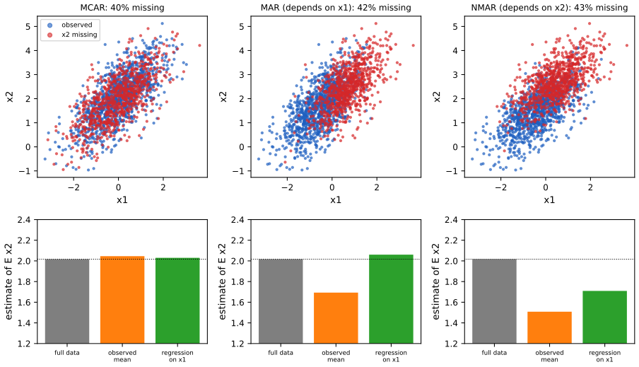
- MCAR (missing completely at random): \(p(\mathbf{M}\given\mathbf{X}_v,\mathbf{X}_h,\mathbf{Y})=p(\mathbf{M})\); nothing the data say affects which values go missing.
- MAR (missing at random): \(p(\mathbf{M}\given\mathbf{X}_v,\mathbf{X}_h,\mathbf{Y})=p(\mathbf{M}\given\mathbf{X}_v,\mathbf{Y})\); it may depend on what was observed but not on the missing values themselves.
- NMAR (not missing at random): neither holds. The absence is itself informative, as when people skip a sensitive question on a survey.
Under MCAR and MAR the mechanism can be ignored when modelling; under NMAR it must be modelled (see Little and Rubin, 1987; Marlin, 2008). The book assumes MAR throughout. Even then, a discriminative model such as a deep network cannot take inputs with holes, and the common heuristic is mean value imputation, replacing each missing entry by the empirical mean of that feature. Better is to fit a generative model of the inputs and use it to fill in the gaps (Chapter 20 and the sequel).
Result 1.5 (when the missingness mechanism can be ignored) p. 27; Rubin (1976)
Let the data distribution be \(p(\mathbf{x}_v,\mathbf{x}_h\given\bm{\theta})\) and the mechanism \(p(\mathbf{m}\given\mathbf{x}_v,\mathbf{x}_h,\bm{\phi})\), with \(\bm{\theta}\) and \(\bm{\phi}\) distinct parameters. If the data are MAR, the likelihood of the observed information \((\mathbf{x}_v,\mathbf{m})\) factorises as \[ p(\mathbf{x}_v,\mathbf{m}\given\bm{\theta},\bm{\phi})=p(\mathbf{m}\given\mathbf{x}_v,\bm{\phi})\ \int p(\mathbf{x}_v,\mathbf{x}_h\given\bm{\theta})\,\d\mathbf{x}_h, \] so inference about \(\bm{\theta}\) can use \(\int p(\mathbf{x}_v,\mathbf{x}_h\given\bm{\theta})\d\mathbf{x}_h\) alone. Under NMAR the factor involving \(\mathbf{x}_h\) stays inside the integral and \(\bm{\theta}\) cannot be separated from \(\bm{\phi}\).
Filling the gap 1.12: proof of Result 1.5 p. 27
The book gives the definitions and the verdict "ignore the mechanism" without the argument.
Proof
The probability of observing the visible values and the pattern \(\mathbf{m}\) is obtained by integrating out the hidden values from the joint, \[ p(\mathbf{x}_v,\mathbf{m}\given\bm{\theta},\bm{\phi})=\int p(\mathbf{m}\given\mathbf{x}_v,\mathbf{x}_h,\bm{\phi})\,p(\mathbf{x}_v,\mathbf{x}_h\given\bm{\theta})\,\d\mathbf{x}_h. \] Under MAR, \(p(\mathbf{m}\given\mathbf{x}_v,\mathbf{x}_h,\bm{\phi})=p(\mathbf{m}\given\mathbf{x}_v,\bm{\phi})\) does not depend on \(\mathbf{x}_h\) and leaves the integral, which is the displayed factorisation. As a function of \(\bm{\theta}\) the likelihood is the second factor up to a constant, so maximum likelihood (or the posterior with independent priors) for \(\bm{\theta}\) does not involve \(\bm{\phi}\). Under NMAR, \(p(\mathbf{m}\given\mathbf{x}_v,\mathbf{x}_h,\bm{\phi})\) varies with \(\mathbf{x}_h\), so the integrand does not factorise; the likelihood of \(\bm{\theta}\) then depends on the model for \(\mathbf{m}\), and a wrong model of the mechanism biases \(\hat{\bm{\theta}}\). ∎
A subtlety. The ignorability argument concerns likelihood-based inference with all observed data used; it does not say that simple methods that discard or fill in values are unbiased under MAR. Result 1.6 shows that the observed mean of a variable is biased under MAR, while the right likelihood-based or regression-based estimate is not.
Result 1.6 (mean imputation and the observed mean) Section 1.5.5 (mean imputation)
Let \((x_1,x_2)\) be bivariate Gaussian with \(\E x_1=0\), \(\var x_1=1\), \(\E x_2=\mu_2\), \(\var x_2=\sigma_2^2\) and correlation \(\rho\), with \(x_1\) always observed and \(x_2\) deleted with probability depending on \(x_1\) or \(x_2\) as stated.
(i) MCAR: the mean of the observed \(x_2\) is unbiased; filling the gaps with it keeps the mean but shrinks the sample variance of \(x_2\) to \(\frac{n_o-1}{n-1}\) times the observed-case variance (about the observed fraction \(\pi=n_o/n\) times \(\sigma_2^2\)) and the correlation with \(x_1\) to about \(\sqrt{\pi}\,\rho\).
(ii) MAR with deletion exactly when \(x_1\gt c\): the observed mean has bias \(-\rho\sigma_2\,\varphi(c)/\Phi(c)\), with \(\varphi,\Phi\) the standard normal density and distribution function; regression of \(x_2\) on \(x_1\) among the complete cases is unbiased.
(iii) NMAR (deletion depends on \(x_2\)): the observed mean is biased and no function of the observed data alone repairs it.
Proof
(i) Under MCAR the observed values are a random subsample, so their mean is unbiased for \(\mu_2\). If the \(n_m=n-n_o\) gaps are filled with the observed mean \(\bar x_o\), the mean of the filled sample is \(\bar x_o\) and its sum of squares about \(\bar x_o\) equals the observed sum of squares (the filled points add zero), so the sample variance is \(\frac{n_o-1}{n-1}s_o^2\approx\pi\,\sigma_2^2\). Similarly the cross-product \(\sum(x_1-\bar x_1)(x_2-\bar x_o)\) over all \(n\) points is about \(\pi n\,\rho\sigma_2\) (the filled points have \(x_2-\bar x_o=0\)); dividing by the standard deviations \(\sqrt{n}\) and \(\sqrt{\pi n}\sigma_2\) gives \(\sqrt\pi\,\rho\). (ii) Writing \(x_2=\mu_2+\rho\sigma_2x_1+\sigma_2\sqrt{1-\rho^2}\,e\) with \(e\) independent standard normal, \(\E[x_2\given x_1\le c]=\mu_2+\rho\sigma_2\E[x_1\given x_1\le c]\), and for a standard normal \(\E[x_1\given x_1\le c]=-\varphi(c)/\Phi(c)\) (integrate \(x\varphi(x)=-\varphi'(x)\)). Because deletion depends only on \(x_1\), the conditional law of \(x_2\) given \(x_1\) is the same in the complete cases, so a regression of \(x_2\) on \(x_1\) among them has the true slope \(\rho\sigma_2\) and intercept \(\mu_2\). Combining it with the full sample of \(x_1\) gives an unbiased estimate of \(\mu_2\): this is the content of Result 1.5 for this model. (iii) If deletion depends on \(x_2\), say removal of the large values, the retained values are a truncated sample whose mean is below \(\mu_2\), and since the missing values are never seen their number and size cannot be recovered without assuming a model of the mechanism. ∎
missing_sample, missing_summary, fig_1_S1. Download: PDF · SVGSee also (companion course): the PCA demo and EM for models with latent or missing variables.
1.6 Discussion
1.6.1 The relationship between ML and other fields
pp. 27–28 The names of neighbouring fields are largely a matter of community. Predictive analytics is close to supervised learning but aimed at business; data mining covers supervised and unsupervised learning on structured data in large commercial databases; data science uses machine learning and statistics but also stresses data integration, visualisation and iteration with domain experts. Machine learning is closely related to statistics: Friedman's remark is that had statistics treated computing as fundamental from the start, many of these fields would have been part of it. It is also related to artificial intelligence: early AI tried to program intelligence by hand, which failed because the needed knowledge is too much to write down, and the current approach is to let systems acquire it by learning.
1.6.2 Structure of the book
p. 28 The book uses probability as one organising thread: foundations in Part I, supervised learning in Parts II to IV, unsupervised learning in Part V. The sequel (Murphy, 2023) covers further topics. Online notebooks accompany the book; this course uses its own code, written from scratch, and the course home page maps the chapters.
1.6.3 Caveats
pp. 28–29 A learned predictor is used to choose actions that minimise expected loss (Result 1.1), but a loss function that fully states our preferences is hard to write; a system may then "hack" the reward, optimising the letter and breaking the spirit. This is one face of the alignment problem: the gap between what we ask a system to optimise and what we want. One proposal is to infer the objective from watching human behaviour (inverse reinforcement learning), recognising that copying behaviour can imitate its biases. A related distinction contrasts autonomous systems (the road to artificial general intelligence) with augmented intelligence, tools such as adaptive cruise control or search autocompletion that keep a person in the loop. If the machine is uncertain about the human's utility it should act cautiously, for example by asking, rather than confidently solving the wrong problem; this is formalised as an assistance game between human and machine.
A tiny numerical illustration of "wrong loss" using Table 1.2: the depth-2 tree of Figure 1.4, labelled for the zero-one loss, has Table 1.2 risk \(0.340\) on the Iris training set, while the same tree labelled by Result 1.1 has \(0.333\) (and a much higher misclassification rate). The point is not the numbers but that the best classifier depends on the loss, so the loss must be chosen with as much care as the model.
Exercises
Chapter 1 of this edition of the book has no end-of-chapter exercises. The four practice problems below, written for these notes, rehearse the chapter's calculations; each has a complete solution (hidden), and each is labelled \(P1\) to \(P4\) rather than numbered like a book exercise.
Practice P1 (decision under Table 1.2). A flower has class probabilities \((p_{\rm Set},p_{\rm Ver},p_{\rm Vir})=(0.55,0.40,0.05)\). Which of the three predictions minimises the expected loss under Table 1.2, and what is that loss? What does the zero-one loss choose?
Solution
By Result 1.1: \(\rho(\text{Setosa})=0.40+10(0.05)=0.90\); \(\rho(\text{Versicolor})=0.55+0.50=1.05\); \(\rho(\text{Virginica})=0.55+0.40=0.95\). The smallest is Setosa with expected loss 0.90, so predict Setosa (the zero-one loss also picks Setosa, the most probable class). Check against the threshold: \(p_3=0.05\lt\max(p_1,p_2)/10=0.055\), so Virginica is not chosen, in agreement. Had \(p_3\) been 0.06 (taking 0.01 from Versicolor) the rule would switch to Virginica: its expected loss would be \(0.55+0.39=0.94\), against \(0.39+0.60=0.99\) for Setosa.
Practice P2 (Gaussian NLL). Show that the average NLL of \(y_n\sim\N(\mathbf{w}^\T\mathbf{x}_n,\sigma^2)\) is minimised jointly by the least squares \(\hat{\mathbf{w}}\) and \(\hat\sigma^2=\MSE(\hat{\mathbf{w}})\), and compute the minimum value.
Solution
By Result 1.2 the average NLL equals \(\MSE(\mathbf{w})/(2\sigma^2)+\tfrac12\log(2\pi\sigma^2)\). For any \(\sigma^2\) it is smallest in \(\mathbf{w}\) at the MSE minimiser \(\hat{\mathbf{w}}\); there it equals \(m/(2\sigma^2)+\tfrac12\log(2\pi\sigma^2)\) with \(m=\MSE(\hat{\mathbf{w}})\), minimised at \(\sigma^2=m\) (Result 1.2(ii)). The minimum value is \(\tfrac12+\tfrac12\log(2\pi m)\). Numerically, for the 21-point stand-in data and a cubic polynomial, minimising the NLL numerically over \(\sigma^2\) gave exactly the MSE of the fit.
Practice P3 (feature crosses). With \(K_1\) levels of the first categorical variable and \(K_2\) of the second, what are the number of columns and the rank of the main-effects encoding, and of the crossed encoding?
Solution
Generalising Filling the gap 1.10: the main-effects design has \(1+K_1+K_2\) columns and rank \(K_1+K_2-1\) (the type indicators sum to the constant and so do the country indicators: two independent relations, so \(1+K_1+K_2-2=K_1+K_2-1\)). With all \(K_1K_2\) cross indicators added, the number of columns is \(1+K_1+K_2+K_1K_2\) and the rank is \(K_1K_2\), the number of cells. For \(K_1=3,K_2=2\): 6 columns of rank 4, and 12 columns of rank 6, as computed.
Practice P4 (mean imputation). A variable has 1000 values of sample variance 4, of which 600 are observed. After mean imputation, what is the sample variance? If its correlation with another fully observed variable was 0.5 among all 1000, what do you expect afterwards under MCAR?
Solution
The observed values have variance \(s_o^2\approx4\); after imputation the variance is \(\frac{n_o-1}{n-1}s_o^2=\frac{599}{999}\cdot4\approx2.40\), so the standard deviation falls from 2 to 1.55. By Result 1.6(i) the correlation falls to about \(\sqrt{0.6}\times0.5\approx0.39\).
Demonstrations for this chapter
Each demonstration runs in the browser, with seeded or stored random numbers so that a class sees the same pictures, and links back to these notes. The ▶ Demo boxes above open them already set to the case under discussion. Each page reproduces the numbers of the Python code (the fits agree to rounding error); they use the same stored samples.
| Demonstration | What you can see | Sections and results |
|---|---|---|
| Polynomial regression: under- and over-fitting | Polynomials of degree 0 to 20 fitted to the 21 points or to a random sample; the fitted curve, the true curve, and training and test MSE for every degree. Presets: 1 degree 2; 2 degree 14; 3 interpolation at degree 20; 4 underfitting; 5 200 points. | 1.2.2.2, 1.2.3, Result 1.3, Figures 1.5, 1.7 |
| Iris decision trees: empirical risk and loss matrices | A Gini tree on any of four feature pairs, depth 0 to 6, fitted on all 150 flowers or on 100 with 50 held out; the zero-one loss against the Table 1.2 loss; leaf probabilities with and without smoothing; click to query. Presets: 1 one split; 2 Figure 1.4; 3 Table 1.2; 4 deep tree; 5 smoothed leaves. | 1.2.1.3 to 1.2.1.5, Result 1.1, Filling the gap 1.1, Figure 1.4 |
| Missing data: MCAR, MAR, NMAR and imputation | A simulated pair \((x_1,x_2)\) with values of \(x_2\) deleted by three mechanisms; the mean, spread and correlation under mean and regression imputation. Presets: 1 MCAR; 2 MAR; 3 NMAR; 4 mean imputation shrinks the spread; 5 regression imputation. | 1.5.5, Result 1.5, Result 1.6, Figure 1.S1 |
The Python code that produces every figure of this page is code/ch01_introduction.py (see the code index).
References
- Murphy, K. P. (2022). Probabilistic Machine Learning: An Introduction. MIT Press, Cambridge, MA. Chapter 1, pp. 1–29. probml.github.io/pml-book/book1.html.
- Murphy, K. P. (2023). Probabilistic Machine Learning: Advanced Topics. MIT Press, Cambridge, MA.
- Cohen, G., Afshar, S., Tapson, J. and van Schaik, A. (2017). EMNIST: extending MNIST to handwritten letters. International Joint Conference on Neural Networks.
- Fisher, R. A. (1936). The use of multiple measurements in taxonomic problems. Annals of Eugenics, 7(2), 179–188.
- Gage, P. (1994). A new algorithm for data compression. The C Users Journal, 12(2), 23–38.
- Krizhevsky, A. and Hinton, G. (2009). Learning multiple layers of features from tiny images. Technical report, University of Toronto.
- LeCun, Y., Bottou, L., Bengio, Y. and Haffner, P. (1998). Gradient-based learning applied to document recognition. Proceedings of the IEEE, 86(11), 2278–2324.
- Little, R. J. A. and Rubin, D. B. (1987). Statistical Analysis with Missing Data. Wiley, New York.
- Maas, A. L., Daly, R. E., Pham, P. T., Huang, D., Ng, A. Y. and Potts, C. (2011). Learning word vectors for sentiment analysis. Proceedings of the 49th Annual Meeting of the Association for Computational Linguistics.
- Marlin, B. M. (2008). Missing Data Problems in Machine Learning. PhD thesis, University of Toronto.
- Mitchell, T. M. (1997). Machine Learning. McGraw-Hill, New York.
- Rajpurkar, P., Zhang, J., Lopyrev, K. and Liang, P. (2016). SQuAD: 100,000+ questions for machine comprehension of text. Proceedings of EMNLP.
- Rubin, D. B. (1976). Inference and missing data. Biometrika, 63(3), 581–592.
- Russakovsky, O. et al. (2015). ImageNet large scale visual recognition challenge. International Journal of Computer Vision, 115(3), 211–252.
- Sennrich, R., Haddow, B. and Birch, A. (2016). Neural machine translation of rare words with subword units. Proceedings of the 54th Annual Meeting of the Association for Computational Linguistics.
- Tipping, M. E. and Bishop, C. M. (1999). Probabilistic principal component analysis. Journal of the Royal Statistical Society, Series B, 61(3), 611–622.
- Wolpert, D. H. (1996). The lack of a priori distinctions between learning algorithms. Neural Computation, 8(7), 1341–1390.
- Xiao, H., Rasul, K. and Vollgraf, R. (2017). Fashion-MNIST: a novel image dataset for benchmarking machine learning algorithms. arXiv:1708.07747.
- Zhang, C., Bengio, S., Hardt, M., Recht, B. and Vinyals, O. (2017). Understanding deep learning requires rethinking generalization. International Conference on Learning Representations.
The numerical statements in the text (the Iris tree and its leaves, the Table 1.2 decision rule, the softmax identities, the Gaussian NLL, the normal equations and interpolation, the optimism \(2\sigma^2p/N\), K-means and PCA optimality, the TF-IDF algebra, the rank of the feature-cross encodings, the finite no-free-lunch average, and the biases and variance shrinkage under missing data) were confirmed numerically.