Causal Inference
"Smokers get more lung cancer" is a statement about association; "smoking causes lung cancer" is a statement about what would happen if we changed someone's smoking. This chapter gives the second kind of statement a precise probabilistic meaning through potential outcomes, the outcomes each subject would have under each treatment, of which we only ever see one. Association and causation then become two different parameters, and the chapter asks when the first identifies the second: always under random assignment, under an untestable "no unmeasured confounding" assumption in observational studies, and never from the data alone otherwise. The book states the main facts briefly. These notes prove them all, and add what the proofs need: the selection bias that separates association from causation, the positivity condition and the uniform consistency that the adjustment formula silently requires, the standard error of the randomised comparison, the substitution argument for continuous treatments, inverse probability weighting, and Simpson's paradox as a statement about two weighted averages.
Ch. 1 Probability Ch. 2 Random variables Ch. 3 Expectation Ch. 4 Inequalities Ch. 5 Convergence Ch. 6 Models and inference Ch. 7 Estimating the CDF Ch. 8 Bootstrap Ch. 9 Parametric inference Ch. 10 Hypothesis testing Ch. 11 Bayesian inference Ch. 12 Decision theory Ch. 13 Regression Ch. 14 Multivariate models Ch. 15 Independence Ch. 16 Causal inference Ch. 17 Directed graphs Ch. 18 Undirected graphs Ch. 19 Log-linear models Ch. 20 Curve estimation Ch. 21 Orthogonal functions Ch. 22 Classification Ch. 23 Stochastic processes Ch. 24 Simulation
How to read these notes
They follow the book. Sections carry the book's numbers (16.1 to 16.6) and every displayed equation that appears in the book carries the book's own equation number, e.g. \((16.7)\). Numbered items keep the book's numbers (Theorem 16.3, Example 16.5, Remark 16.7); definitions and results the book states without a number, and the new results needed to fill its gaps, are lettered (Definition 16.A, Theorem 16.B, ...). Equations without a number are steps that the book skips.
Filling the gaps. Wherever the book says "it can be shown", quotes a result without proof, or leaves an argument implicit, an orange Filling the gap box gives the full argument. Proofs and derivations start hidden: open one with its bar, or use the button below.
Figures and demonstrations. The chapter's two figures are drawn with counterfactual curves of my own (Figures 16.1 and 16.2), and five supplementary figures (16.S1 to 16.S5) illustrate the gaps filled in the notes; all are computed by the Python code. The ▶ Demo boxes open an interactive demonstration already set to the case being discussed.
Main reference
L. Wasserman, All of Statistics: A Concise Course in Statistical Inference, Springer (2004), Chapter 16, pages 251–262 (book website: www.stat.cmu.edu/~larry/all-of-statistics). Section, equation, example and exercise numbers below refer to this book. Further reading is listed in the references.
The explanations, derivations, figures and code are my own; equations are cited by their numbers in the book.
Companion courses
Causal questions appear in three companion courses on this site. The overlapping material is:
- Statistical Methods for Modern Biology, Chapter 13 (design of experiments): Filling the gap 13.1 writes an observational comparison as a causal effect plus a selection bias (the same decomposition as Filling the gap 16.2 here, for the effect on the treated); Section 13.4.1 and Filling the gap 13.7 treat confounding as non-identifiability and derive the omitted-variable bias; Filling the gap 13.12 proves Neyman's (1923) result that randomisation makes the difference in means unbiased for a fixed set of units, with its exact variance, the finite-population version of Theorem 16.3. Its paired design demo shows blocking at work.
- Applied Statistical Learning in R and Python, Filling the gap 4.3: a coefficient that changes sign when a confounder is added, which is Simpson's paradox in a logistic regression.
- Foundations of Deep Learning, Section 11.1 (directed graphical models, Definition 11.1) and Section 11.2 (conditional independence and d-separation), and Bayesian and Probabilistic Machine Learning, Section 8.1: the directed graphs that the book uses for causation in its next chapter.
Those courses take the potential-outcome model or the graph as given and use it for design or for computation; this chapter builds the model from scratch and asks what the observable distribution can and cannot say about it. Where a proof there is identical, these notes give the statement and a short argument and link to it. New here: the four response types and what the data cannot identify (Filling the gap 16.1), the large-sample theory of the randomised comparison (16.3), continuous treatments (16.5), the adjustment formula with positivity (16.6), consistency of plug-in and regression estimators and what regression estimates when the effect varies (16.7), inverse probability weighting (16.8) and Simpson's paradox (16.9, 16.10).
The chapter at a glance
- 16.1 Potential outcomes \((C_0,C_1)\) and the consistency relation \(Y=C_X\) (Definition 16.A); the causal effect \(\th\) and the association \(\alpha\) (Definition 16.B) differ in general (Theorem 16.1, Example 16.2) by a selection bias (Filling the gap 16.2), and coincide under random assignment (Theorem 16.3).
- 16.2 A dose \(x\) has a counterfactual curve \(C(x)\); the causal regression \(\th(x)=\E C(x)\) differs from \(r(x)=\E(Y\given X=x)\) unless the dose is randomised (Theorem 16.4, Example 16.5).
- 16.3 If treatment is as good as random within strata of measured \(Z\) (16.6), the adjusted treatment effect (16.7) identifies \(\th(x)\) (Theorem 16.6), provided every stratum can receive every treatment (positivity); it is estimated by averaging a regression over the observed \(Z\) (16.7) or by weighting (16.8).
- 16.4 Simpson's paradox: a treatment can look better within every group and worse overall, because the two arms average over different mixes of the groups (16.9); a treatment that truly helps every group helps overall (16.10).
Notation. \(X\) is the treatment, \(Y\) the observed outcome and \(Z\) a covariate; \(C_0,C_1\) (or \(C(x)\), \(x\in\cX\)) are the potential outcomes. \(A\indep B\) means \(A\) and \(B\) are independent and \(A\indep B\given Z\) conditionally independent given \(Z\). We write \(p_1=\P(X=1)\), \(p_0=1-p_1\), \(F_Z\) for the distribution of \(Z\), \(e(z)=\P(X=1\given Z=z)\) for the propensity score, \(\bY_1,\bY_0\) for the treated and untreated sample means, \(\pto\) for convergence in probability and \(\dto\) for convergence in distribution. All outcomes are assumed to have finite means.
Prerequisites. Independence and conditional independence (Chapter 2), the law of total probability (Theorem 1.16), conditional expectation and iterated expectations (Result 3.11), the law of large numbers, Slutsky's theorem and the central limit theorem (Theorems 5.6, 5.5 and 5.8), and least squares (Chapter 13 of the book). See the course home.
16.1 The Counterfactual Model
p. 251 Informally, "\(X\) causes \(Y\)" means that changing the value of \(X\) changes the distribution of \(Y\). A causal \(X\) is associated with \(Y\), but an associated \(X\) need not be causal. To tell the two apart we need more random variables than \((X,Y)\). Let \(X\in\{0,1\}\) be a treatment (\(X=1\): treated), understood broadly: a drug, an exposure such as smoking, a policy. Let \(Y\) be an outcome, such as recovery.
Definition 16.A (potential outcomes; the consistency relation) pp. 251–252
Each subject carries two potential outcomes: \(C_0\), the outcome it would have if untreated, and \(C_1\), the outcome it would have if treated. The observed outcome is the potential outcome of the treatment actually received,
\[ Y=C_X=\begin{cases}C_0 & X=0,\\ C_1 & X=1.\end{cases} \tag{16.1} \]Equation (16.1) is the consistency relation. The potential outcome of the treatment not received is counterfactual: it is what would have happened, contrary to fact.
A small data set makes the bookkeeping concrete. Eight subjects, four untreated and four treated, with observed outcomes; the asterisks mark counterfactuals, which are never observed.
| \(X\) | 0 | 0 | 0 | 0 | 1 | 1 | 1 | 1 |
|---|---|---|---|---|---|---|---|---|
| \(Y\) | 4 | 7 | 2 | 8 | 3 | 5 | 8 | 9 |
| \(C_0\) | 4 | 7 | 2 | 8 | * | * | * | * |
| \(C_1\) | * | * | * | * | 3 | 5 | 8 | 9 |
Half of every subject's pair \((C_0,C_1)\) is missing, so causal inference is a missing-data problem in which the missingness is caused by the treatment choice. With binary outcomes each subject is one of four types: survivors \((C_0,C_1)=(1,1)\), responders \((0,1)\), anti-responders \((1,0)\) and the doomed \((0,0)\). Think of \((C_0,C_1)\) as a hidden variable that records everything about the subject that matters for the outcome.
Filling the gap 16.1: what (16.1) assumes, and what the data can never tell p. 252
(a) The assumptions inside (16.1). Writing \(Y=C_X\) presumes that a subject's outcome depends only on its own treatment (no interference: my vaccination does not change your \(C_0\)) and that "treated" means one well-defined intervention (if two doses both count as \(X=1\), \(C_1\) is not one number). Together these are often called the stable unit treatment value assumption. Algebraically, for binary \(X\),
\[ Y=XC_1+(1-X)C_0 . \](b) The causal effect in terms of types. With binary outcomes and type proportions \(\pi_S,\pi_R,\pi_A,\pi_D\),
\[ \E(C_1)-\E(C_0)=\pi_R-\pi_A : \]the average causal effect counts responders minus anti-responders. Survivors and the doomed contribute nothing whatever they receive.
(c) The joint law of \((C_0,C_1)\) is never identified. Even with perfect randomisation the data reveal at most the two margins \(\P(C_1=1)\) and \(\P(C_0=1)\), never the share of responders. Given the margins, \(\pi_R\) can be anything in the Fréchet interval
\[ \max\{0,\ \P(C_1=1)-\P(C_0=1)\}\ \le\ \pi_R\ \le\ \min\{\P(C_1=1),\ \P(C_0=0)\}, \]and both ends are attained. For example, \(\P(C_1=1)=0.5\) and \(\P(C_0=1)=0.3\) are produced both by \((\pi_S,\pi_R,\pi_A,\pi_D)=(0.3,0.2,0,0.5)\), with 20% responders, and by \((0,0.5,0.3,0.2)\), with 50% responders and 30% anti-responders. Both give \(\th=0.2\); the average effect is identifiable, the distribution of individual effects is not.
Derivations
(a) If \(X=1\) the right side is \(C_1\), if \(X=0\) it is \(C_0\).
(b) \(\E C_1=\P(C_1=1)=\pi_S+\pi_R\) and \(\E C_0=\pi_S+\pi_A\); subtract.
(c) Each subject is observed under one treatment only, so no data set, however large, contains a single pair \((C_0,C_1)\): the observable distribution is a function of the law of \((X,C_X)\), which under randomisation depends on the law of \((C_0,C_1)\) only through its margins (Theorem 16.3). Write \(a=\P(C_1=1)=\pi_S+\pi_R\) and \(b=\P(C_0=1)=\pi_S+\pi_A\). Given \(a,b\), the four proportions are determined by \(\pi_R\): \(\pi_S=a-\pi_R\), \(\pi_A=b-a+\pi_R\), \(\pi_D=1-b-\pi_R\). They are all nonnegative exactly when \(\pi_R\le a\), \(\pi_R\ge a-b\), \(\pi_R\ge0\) and \(\pi_R\le1-b\), which is the interval stated; every point of it gives a valid population with the same margins. In the example \(a=0.5\), \(b=0.3\) give the interval \([0.2,0.5]\). ∎
Definition 16.B (causal effect and association) pp. 252–253
The average causal effect (or average treatment effect) is
\[ \th=\E(C_1)-\E(C_0), \tag{16.2} \]the mean outcome if everyone were treated minus the mean outcome if no one were. For binary potential outcomes two other causal summaries are the causal odds ratio and the causal relative risk,
\[ \frac{\P(C_1=1)}{\P(C_1=0)}\Big/\frac{\P(C_0=1)}{\P(C_0=0)}\qquad\text{and}\qquad\frac{\P(C_1=1)}{\P(C_0=1)} . \]The association is
\[ \alpha=\E(Y\given X=1)-\E(Y\given X=0). \tag{16.3} \]The ideas below do not depend on which summary is used; we work with \(\th\) and \(\alpha\).
Theorem 16.1 (association is not causation) p. 253
In general, \(\th\ne\alpha\).
Example 16.2. pp. 253–254 Take a population of eight people, four of each of two types:
| \(X\) | 0 | 0 | 0 | 0 | 1 | 1 | 1 | 1 |
|---|---|---|---|---|---|---|---|---|
| \(Y\) | 0 | 0 | 0 | 0 | 1 | 1 | 1 | 1 |
| \(C_0\) | 0 | 0 | 0 | 0 | 1* | 1* | 1* | 1* |
| \(C_1\) | 0* | 0* | 0* | 0* | 1 | 1 | 1 | 1 |
Every subject has \(C_0=C_1\), so the treatment changes nobody's outcome and \(\th=\tfrac48-\tfrac48=0\). But the observed data give \(\alpha=\tfrac44-\tfrac04=1\). Read \(Y=1\) as "healthy" and \(X=1\) as "takes vitamin C": healthy people (survivors) take vitamin C and unhealthy ones (the doomed) do not, and it is this link between type and treatment that produces the association. A naive observer who reads \(\alpha=1\) causally and persuades three of the four unhealthy people to take vitamin C produces the population
| \(X\) | 0 | 1 | 1 | 1 | 1 | 1 | 1 | 1 |
|---|---|---|---|---|---|---|---|---|
| \(Y\) | 0 | 0 | 0 | 0 | 1 | 1 | 1 | 1 |
in which \(\alpha=\tfrac47-\tfrac01=\tfrac47\). The association has dropped from 1 to \(4/7\) although nothing causal has changed, and the advice seems to have made things worse. It is not hard to build populations in which \(\alpha>0\) and \(\th<0\) (Exercise 16.1). The source of the discrepancy is that \((C_0,C_1)\) is not independent of \(X\): the choice of treatment depends on the type of person.
Filling the gap 16.2: association = causation + selection bias pp. 253–254
Assume \(0<p_1<1\). Measure how much the treated and untreated groups differ in their potential outcomes by
\[ D_1=\E(C_1\given X=1)-\E(C_1\given X=0),\qquad D_0=\E(C_0\given X=1)-\E(C_0\given X=0). \]Then, exactly,
\[ \alpha-\th=p_0D_1+p_1D_0 . \]Consequences. (i) \(\alpha=\th\) whenever \(D_0=D_1=0\), i.e. whenever both potential outcomes are mean independent of \(X\); full independence is not needed. (ii) \(\alpha\) and \(\th\) can have opposite signs: in Example 16.2 \(D_0=D_1=1\) and \(\alpha=\th+1\). (iii) If people choose the treatment that is better for them, the treated are those with high \(C_1\) and the untreated those with high \(C_0\), and the bias can have either sign. The companion course writes the same decomposition for the effect on the treated (Statistical Methods for Modern Biology, Filling the gap 13.1).
In the four-type model with treatment probabilities \(e_t=\P(X=1\given\text{type }t)\), the arms contain the types in proportions \(\pi_te_t/p_1\) and \(\pi_t(1-e_t)/p_0\). For \(\pi=(0.3,0.2,0.1,0.4)\) (survivors, responders, anti-responders, doomed) and \(e=(0.9,0.3,0.6,0.15)\): \(\th=0.2-0.1=0.1\), \(p_1=0.45\), \(\E(Y\given X=1)=0.733\), \(\E(Y\given X=0)=0.127\), so \(\alpha=0.606\); and \(D_1=0.424\), \(D_0=0.606\), giving \(p_0D_1+p_1D_0=0.506=\alpha-\th\). The causal relative risk is 1.25 while the associational one is 5.76.
Derivation
By the consistency relation, \(\E(Y\given X=1)=\E(C_1\given X=1)\) and \(\E(Y\given X=0)=\E(C_0\given X=0)\). By the law of total expectation (Result 3.11),
\[ \E C_1=p_1\E(C_1\given X=1)+p_0\E(C_1\given X=0),\qquad\text{so}\qquad \E(C_1\given X=1)-\E C_1=p_0D_1 ; \] \[ \E C_0=p_1\E(C_0\given X=1)+p_0\E(C_0\given X=0),\qquad\text{so}\qquad \E(C_0\given X=0)-\E C_0=-p_1D_0 . \]Hence \(\alpha-\th\)
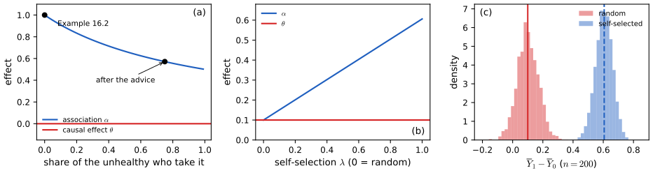
fig_16_s1. Download: PDF · SVGp. 254 Can a causal effect ever be estimated? Sometimes: random assignment makes it possible.
Theorem 16.3 (randomisation identifies the causal effect) pp. 254–255
Suppose subjects are assigned to treatment at random, with \(\P(X=0)>0\) and \(\P(X=1)>0\). Then \(\alpha=\th\). Hence any consistent estimator of \(\alpha\) is a consistent estimator of \(\th\); in particular
\[ \ht=\widehat\E(Y\given X=1)-\widehat\E(Y\given X=0)=\bY_1-\bY_0,\qquad \bY_1=\frac1{n_1}\sum_{i=1}^nY_iX_i,\quad \bY_0=\frac1{n_0}\sum_{i=1}^nY_i(1-X_i), \]with \(n_1=\sum_iX_i\) and \(n_0=\sum_i(1-X_i)\), is consistent for \(\th\).
The book's proof. Random assignment makes \(X\) independent of \((C_0,C_1)\), so \(\th\)
Filling the gap 16.3: the randomised comparison, rigorously: consistency, standard error, confidence interval pp. 254–255
Let \((X_i,C_{0i},C_{1i})\), \(i=1,\dots,n\), be IID with \(X\indep(C_0,C_1)\), \(0<p_1<1\), \(\sigma_x^2=\V(C_x)<\infty\), and \(Y_i=C_{X_i,i}\). Set \(\ht=\bY_1-\bY_0\) when both arms are nonempty (any value otherwise). Then
- Identification: \(\E(Y\given X=x)=\E(C_x\given X=x)=\E(C_x)\), so \(\alpha=\th\).
- Consistency: \(\ht\pto\th\).
- Asymptotic normality: \(\sqrt n(\ht-\th)\dto\N\big(0,\ \sigma_1^2/p_1+\sigma_0^2/p_0\big)\).
- Confidence interval: with \(s_x^2\) the sample variance in arm \(x\), \(\ht\pm z_{\alpha/2}\sqrt{s_1^2/n_1+s_0^2/n_0}\) has coverage tending to \(1-\alpha\).
Only mean independence is needed for 1 and 2; the variance in 3 uses only that each arm is an IID sample from the corresponding potential-outcome distribution. For binary outcomes \(\sigma_x^2=\mu_x(1-\mu_x)\) with \(\mu_x=\E C_x\). In the population of Filling the gap 16.2 under random assignment (\(p_1=0.45\), \(\mu_1=0.5\), \(\mu_0=0.4\)) and \(n=200\), the standard deviation of \(\ht\) is about \(\sqrt{0.25/90+0.24/110}=0.070\); 1000 simulated studies give 0.070, and the 95% Wald interval covers \(\th=0.1\) in 94.5% of 4000 simulated studies of \(n=400\).
See also (companion course): for a fixed set of \(N\) units with fixed potential outcomes, randomising exactly \(n_1\) of them to treatment makes \(\ht\) exactly unbiased for the average effect of those units, with variance \(S_1^2/n_1+S_0^2/n_0-S_\tau^2/N\) (Neyman, 1923); the proof is Filling the gap 13.12 of Statistical Methods for Modern Biology. The last term, the variance of the individual effects, is never estimable (Filling the gap 16.1(c)), so the usual variance estimate is conservative there.
Derivations
(1) For \(x\in\{0,1\}\) and \(\P(X=x)>0\): on \(\{X=x\}\) we have \(Y=C_x\) by (16.1), so \(\E(Y\given X=x)\)
(2) Write \(\bY_1=\frac{n^{-1}\sum_iY_iX_i}{n^{-1}\sum_iX_i}\). By the weak law of large numbers (Theorem 5.6) the numerator tends in probability to \(\E(YX)=\E(C_1X)=\mu_1p_1\) and the denominator to \(p_1>0\); the ratio is a continuous function away from 0, so \(\bY_1\pto\mu_1\) (Theorem 5.5). Similarly \(\bY_0\pto\mu_0\). The event that an arm is empty has probability \(p_1^n+p_0^n\to0\), so the arbitrary value used there does not matter. Hence \(\ht\pto\mu_1-\mu_0=\th\).
(3) Let
\[ W_i=\frac{X_i(Y_i-\mu_1)}{p_1}-\frac{(1-X_i)(Y_i-\mu_0)}{p_0} . \]Then \(\E W_i=0\) and, since \(X_i(1-X_i)=0\),
\[ \V(W_i)=\frac{\E[X(C_1-\mu_1)^2]}{p_1^2}+\frac{\E[(1-X)(C_0-\mu_0)^2]}{p_0^2}=\frac{\sigma_1^2}{p_1}+\frac{\sigma_0^2}{p_0}, \]using independence once more. Now \(\bY_1-\mu_1\)
by the central limit theorem (Theorem 5.8) and Slutsky's theorem: the remainder is \(\frac1{\sqrt n}\sum X_i(Y_i-\mu_1)\cdot(\frac n{n_1}-\frac1{p_1})\), a product of a term bounded in probability and one tending to 0.
(4) \(s_x^2\pto\sigma_x^2\) and \(n_x/n\pto p_x\), so \(n(s_1^2/n_1+s_0^2/n_0)\pto\sigma_1^2/p_1+\sigma_0^2/p_0\); combine with (3) and Slutsky's theorem as in Theorem 5.10. ∎
p. 255 If \(Z\) is a covariate, the conditional causal effect is
\[ \th_z=\E(C_1\given Z=z)-\E(C_0\given Z=z). \]If \(Z\) is sex, \(\th_0\) is the effect among women and \(\th_1\) among men. In a randomised experiment, \(\th_z=\E(Y\given X=1,Z=z)\)
Filling the gap 16.4: conditional effects in a randomised experiment, and why \(Z\) must be a pre-treatment covariate p. 255
Claim. If \(X\indep(C_0,C_1,Z)\) jointly and \(\P(X=x,Z=z)>0\), then \(\E(Y\given X=x,Z=z)=\E(C_x\given Z=z)\), so \(\th_z\) is the difference of the two conditional means, and \(\th=\E(\th_Z)\). Physical randomisation gives the joint independence for every covariate \(Z\) fixed before treatment.
Independence of \(X\) and \((C_0,C_1)\) alone is not enough. Let \(C_0=C_1=U\) with \(U\sim\Bern(1/2)\), \(X\sim\Bern(1/2)\) independent of \(U\), and \(Z=U\oplus X\) (addition modulo 2). Then \(X\indep(C_0,C_1)\) and every conditional effect is \(\th_z=0\), yet given \(Z=0\) the treated have \(Y=1\) and the untreated \(Y=0\), so the within-group difference is 1. Here \(Z\) depends on the treatment: conditioning on a variable measured after treatment can manufacture an effect (see also Filling the gap 16.10).
Post-stratification. When \(Z\) is discrete, \(\sum_z\frac{n_z}{n}(\bY_{1z}-\bY_{0z})\) estimates \(\th\) as well, often more precisely than \(\bY_1-\bY_0\), because it removes the variation of the outcome across groups; this is the stratified estimator of Filling the gap 16.7.
Derivation
Joint independence gives \(X\indep(C_x,Z)\), hence \(\P(X=x\given C_x,Z)=\P(X=x)\) and \(X\indep C_x\given Z\). Then \(\E(Y\given X=x,Z=z)\)
Summary of the counterfactual model p. 255
Random variables \((C_0,C_1,X,Y)\); consistency \(Y=C_X\); causal effect \(\th=\E C_1-\E C_0\); association \(\alpha=\E(Y\given X=1)-\E(Y\given X=0)\); random assignment \(\Rightarrow(C_0,C_1)\indep X\Rightarrow\th=\alpha\).
16.2 Beyond Binary Treatments
pp. 255–256 Now let \(X\in\cX\) be general, for instance a dose with \(\cX\subseteq\R\). The pair \((C_0,C_1)\) becomes a counterfactual function \(C(x)\), the outcome the subject would have at dose \(x\), and the consistency relation is
\[ Y\equiv C(X): \tag{16.4} \]we observe the curve at the one dose actually received (Figure 16.1). The causal regression function and the ordinary regression function are
\[ \th(x)=\E\big(C(x)\big),\tag{16.5} \] \[ r(x)=\E(Y\given X=x). \]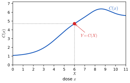
fig_16_1. Download: PDF · SVGTheorem 16.4 p. 256
In general \(\th(x)\ne r(x)\). When \(X\) is randomly assigned, \(\th(x)=r(x)\).
Filling the gap 16.5: proof of Theorem 16.4 for a continuous dose (the substitution lemma) p. 256; Exercise 16.2
For a binary treatment the proof of Theorem 16.3 conditions on events \(\{X=x\}\) of positive probability. For a continuous dose \(\P(X=x)=0\), and "substituting \(X=x\) into \(C(X)\)" needs an argument.
Setting. \(C(x,\omega)\) is jointly measurable in \((x,\omega)\), \(\E|C(x)|<\infty\) for every \(x\), \(m(x)=\E C(x)=\th(x)\) is measurable, \(\E|C(X)|<\infty\), and random assignment means that \(X\) is independent of the whole process \(\{C(x):x\in\cX\}\).
Substitution lemma. Under these conditions, \(\E\big(C(X)\given X\big)=m(X)\) almost surely. Hence \(r(x)=\th(x)\) for \(F_X\)-almost every \(x\) (a regression function is only defined up to such null sets; if both are continuous, for every \(x\) in the support of \(X\)).
Without randomisation, \(r(x)-\th(x)=\E(C(x)\given X=x)-\E C(x)\): the curves of those who chose dose \(x\) need not be typical curves. Example 16.5 and Figure 16.S4 below show this.
Proof
Let \(h\) be bounded and measurable. Because \(X\) and the process \(C\) are independent, the joint law of \((X,C)\) is the product of their laws, so by Fubini's theorem (applied first to \(|C(x)h(x)|\), whose iterated integral is finite by the integrability assumption)
\[ \E\big[C(X)h(X)\big]=\int\Big(\int C(x,\omega)\,\P(\d\omega)\Big)h(x)\,F_X(\d x)=\int m(x)h(x)\,F_X(\d x)=\E\big[m(X)h(X)\big]. \]This holds for every bounded measurable \(h\), which is the defining property of \(\E(C(X)\given X)=m(X)\). Since \(Y=C(X)\) by (16.4), \(r(X)=\E(Y\given X)=m(X)=\th(X)\) almost surely. ∎
A simulation with \(C(x)=A+\sin x\), \(A\sim\N(2,1)\): a dose drawn uniformly on \([0,4]\) independently of \(A\) gives binned regression values within 0.02 of \(\th(x)=2+\sin x\); a dose that decreases with \(A\) gives values off by more than 0.5.
Example 16.5. pp. 256–258 Figure 16.2 shows four subjects whose counterfactual curves are flat: \(C_i(x)=c_i\) for every dose, so no subject's outcome depends on the dose and \(\th(x)=\tfrac14\sum_ic_i\) is constant. The subjects chose different doses, the one with the highest curve the lowest dose. The observed points \(Y_i=C_i(X_i)\) then lie on a decreasing line: there is association without causation.
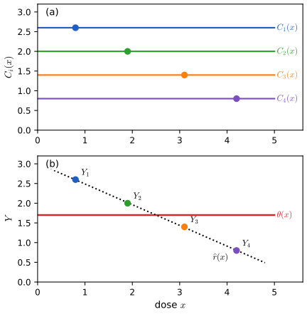
fig_16_2. Download: PDF · SVG16.3 Observational Studies and Confounding
p. 257 In an observational study the treatment is not assigned by the investigator: subjects select their own exposure. Most health studies reported in the press are of this kind. As we have seen, association and causation can then differ, because \(C\) is not independent of \(X\). Suppose, however, that we can form groups of subjects so similar (in age, sex, education, background, ...) that within a group the choice of \(X\) is effectively random. The grouping variables are confounding variables; collect them in \(Z\). The idea is
\[ \{C(x):x\in\cX\}\indep X\given Z . \tag{16.6} \]Within levels of \(Z\), the treatment choice does not depend on the subject's type. If (16.6) holds and \(Z\) is observed, there is no unmeasured confounding. (The book gives a sharper definition of confounding in its next chapter, with graphs.)
Theorem 16.6 (the adjusted treatment effect) p. 257
Suppose (16.6) holds (and the positivity condition of Filling the gap 16.6). Then
\[ \th(x)=\int\E(Y\given X=x,Z=z)\,\d F_Z(z). \tag{16.7} \]If \(\hr(x,z)\) is a consistent estimate of \(r(x,z)=\E(Y\given X=x,Z=z)\) (in the sense of Filling the gap 16.7), then a consistent estimate of \(\th(x)\) is
\[ \ht(x)=\frac1n\sum_{i=1}^n\hr(x,Z_i). \]As printed, (16.7) has an extra "\(\d z\)" after \(\d F_Z(z)\); the version above is the corrected one (Notes on the book).
Filling the gap 16.6: proof of (16.7), and the positivity condition it needs p. 257, Remark 16.7
Positivity. \(\E(Y\given X=x,Z=z)\) must be defined for \(F_Z\)-almost every \(z\): for a discrete treatment, \(\P(X=x\given Z=z)>0\) for almost every \(z\); for a continuous dose, the conditional density of \(X\) given \(Z=z\) must be positive at \(x\). Without it the data contain no subject with \(Z=z\) at dose \(x\), and \(\th(x)\) is not identified: if no one in a stratum is ever treated, the stratum's \(C_1\) can be anything without changing the distribution of the data.
Discrete form. For finitely many strata, (16.7) reads \(\th(x)=\sum_z\E(Y\given X=x,Z=z)\P(Z=z)\), the standardised mean: the stratum-specific means of dose \(x\), averaged with the stratum frequencies of the whole population.
Comparison with association (Remark 16.7). The ordinary regression averages the same stratum means with the strata of those who received \(x\):
\[ r(x)=\int\E(Y\given X=x,Z=z)\,\d F_{Z\given X}(z\given x),\qquad r(x)-\th(x)=\int\E(Y\given X=x,Z=z)\,\big[\d F_{Z\given X}(z\given x)-\d F_Z(z)\big]. \]The two coincide when \(Z\indep X\) (the mixes agree, as under randomisation) or when \(\E(Y\given X=x,Z=z)\) does not depend on \(z\) (the mixes do not matter). Confounding needs both a \(Z\) that predicts treatment and a \(Z\) that predicts outcome.
Proof
By the consistency relation, on \(\{X=x\}\) we have \(Y=C(x)\), so \(\E(Y\given X=x,Z=z)\)
The expression for \(r(x)\) is iterated expectations conditional on \(X=x\). Positivity counterexample: two strata of equal size, the first never treated. Model (a) has \(C_1=C_0+1\) in both strata; model (b) has \(C_1=C_0+3\) in the first and \(C_1=C_0+1\) in the second. The observable law (which involves only \(C_0\) in the first stratum) is the same, but \(\th=1\) in (a) and \(\th=2\) in (b). ∎
p. 259 In particular, if \(r(x,z)=\beta_0+\beta_1x+\beta_2z\) is linear, a consistent estimate of \(\th(x)\) is
\[ \ht(x)=\widehat\beta_0+\widehat\beta_1x+\widehat\beta_2\bZ_n, \tag{16.8} \]with \((\widehat\beta_0,\widehat\beta_1,\widehat\beta_2)\) the least-squares estimates.
Filling the gap 16.7: when the plug-in estimate is consistent, and what regression estimates when its model is wrong pp. 257–259
Theorem 16.C (consistency of the plug-in estimate). Suppose \(\int|r(x,z)|\,\d F_Z(z)<\infty\) and the regression estimate is uniformly consistent, \(\sup_z|\hr(x,z)-r(x,z)|\pto0\) (or, more generally, \(\frac1n\sum_i|\hr(x,Z_i)-r(x,Z_i)|\)
Discrete \(Z\): the stratified estimator. With finitely many strata and the stratum means as \(\hr\), the plug-in estimate is
\[ \ht=\sum_z\frac{n_z}{n}\big(\bY_{1z}-\bY_{0z}\big), \]the stratum differences averaged with the stratum frequencies. It is consistent under (16.6) and positivity, because each stratum mean is a ratio of averages (as in Filling the gap 16.3) and there are finitely many.
(16.8) is a plug-in estimate. For the linear fit, \(\frac1n\sum_i(\widehat\beta_0+\widehat\beta_1x+\widehat\beta_2Z_i)\)
When the effect varies with \(Z\). If the true regression has an interaction, \(r(x,z)=\beta_0+\beta_1x+\beta_2z+\beta_3xz\), then \(\th(1)-\th(0)=\beta_1+\beta_3\E Z\), but the least-squares coefficient of \(X\) in the fit without interaction converges to a weighted average of the stratum effects with weights that depend on the propensity, not on \(F_Z\). With stratum indicators instead of a linear \(z\) (a saturated model for the baseline), the weights are exactly proportional to \(\P(Z=z)\,e(z)\{1-e(z)\}\): strata where treatment is close to a coin toss count most. In the adjustment demo's model with three strata, propensities \(0.047,0.269,0.731\) and stratum effects \(-0.5,1,2.5\) (so \(\th=1\)), the regression (16.8) converges to 1.599 and the regression on stratum indicators to 1.518, while the stratified estimator converges to 1. Adding the interaction to the model, or stratifying, removes the bias.
Proofs
Theorem 16.C. Write
\[ \ht(x)-\th(x)=\frac1n\sum_i\{\hr(x,Z_i)-r(x,Z_i)\}+\Big\{\frac1n\sum_ir(x,Z_i)-\th(x)\Big\}. \]The first term is at most \(\frac1n\sum_i|\hr(x,Z_i)-r(x,Z_i)|\), which is at most \(\sup_z|\hr(x,z)-r(x,z)|\pto0\). The second tends to 0 in probability by the weak law of large numbers, since \(r(x,Z_i)\) are IID with mean \(\int r(x,z)\,\d F_Z(z)=\th(x)\) by (16.7).
(16.8). Linearity of the average. If \(r\) is linear and \(\V(\epsilon\given X,Z)\) is bounded, least squares is consistent for \(\beta\) (Chapter 13 of the book), \(\bZ_n\pto\E Z\), and the continuous mapping theorem gives \(\ht(x)\pto\beta_0+\beta_1x+\beta_2\E Z\)
Interaction. Under the interaction model, (16.7) gives \(\th(x)=\beta_0+\beta_2\E Z+(\beta_1+\beta_3\E Z)x\). Weights with stratum indicators. Regress \(Y\) on \(X\) and indicators of the strata. By the Frisch-Waugh theorem the coefficient of \(X\) equals \(\Cov(\tilde X,Y)/\V(\tilde X)\) in the limit, where \(\tilde X=X-e(Z)\) is the residual of \(X\) after projecting on the stratum indicators (the projection is exact because the indicators span all functions of \(Z\)). Since \(\E(Y\given X,Z)=\mu_0(Z)+\tau(Z)X\), and \(\E[\tilde X\mu_0(Z)]=0\),
\[ \Cov(\tilde X,Y)=\E\big[\tilde X\,\tau(Z)X\big]=\E\big[\tau(Z)\,e(Z)\{1-e(Z)\}\big],\qquad \V(\tilde X)=\E\big[e(Z)\{1-e(Z)\}\big]. \]With a linear term in \(z\) instead of indicators, the projection of \(X\) on \((1,z)\) is not \(e(Z)\) in general and the weights change again; they happen to give \(\th\) when the propensities are symmetric about the middle stratum with three strata, which is why the demo's model puts a quarter of the middle stratum, not a half, under treatment. ∎
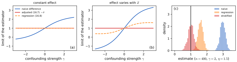
fig_16_s2. Download: PDF · SVGSee also (companion course): the omitted-variable bias of a regression that leaves out a confounder, and complete confounding as non-identifiability, in Statistical Methods for Modern Biology, Filling the gap 13.7.
The same logic works for a continuous dose. In Figure 16.S4 every subject's curve is \(C_i(x)=A_i+0.5x\), increasing in the dose, but subjects with a high baseline \(A_i\) (driven by a confounder \(Z_i\)) choose low doses. The least-squares line of \(Y\) on \(X\) then slopes downward, \(r(x)=7.19-0.54x\), while the adjusted estimate (16.8), which also uses \(Z\), recovers \(\th(x)=2+0.5x\).
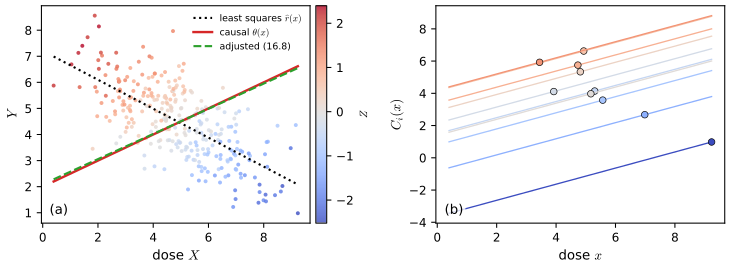
fig_16_s4. Download: PDF · SVGFilling the gap 16.8: weighting instead of regression (inverse probability weighting) p. 258
For a binary treatment, under (16.6) and positivity \(0<e(z)<1\), the adjusted effect has a second expression that needs no outcome model:
\[ \E C_1=\E\Big[\frac{XY}{e(Z)}\Big],\qquad \E C_0=\E\Big[\frac{(1-X)Y}{1-e(Z)}\Big]. \]Weighting each treated subject by \(1/e(Z)\) rebuilds the whole population from the treated (Horvitz and Thompson, 1952; Robins, 1986). Two further facts:
- For discrete \(Z\), weighting and stratifying agree exactly. With \(e(z)\) estimated by the stratum treated fraction \(n_{1z}/n_z\), the weighting estimator equals the stratified estimator \(\sum_z\frac{n_z}{n}(\bY_{1z}-\bY_{0z})\) (when every stratum has both arms).
- The propensity score is enough (Rosenbaum and Rubin, 1983). If (16.6) holds given \(Z\), it also holds given the one-dimensional \(e(Z)\): \((C_0,C_1)\indep X\given e(Z)\). One can stratify or match on \(e(Z)\) instead of on all of \(Z\).
Weights near \(1/0\) are the price of weak positivity: when some \(e(z)\) is close to 0 or 1, the weighting estimator (and the stratified one) becomes very variable, which the adjustment demo shows in preset 5.
Derivations
By (16.1), \(XY=XC_1\). Conditioning on \(Z\) and using (16.6), \(\E[XC_1\given Z]\)
(1) With \(\widehat e(z)=n_{1z}/n_z\), \(\frac1n\sum_i\frac{X_iY_i}{\widehat e(Z_i)}\)
(2) It suffices to show \(\P(X=1\given C_0,C_1,e(Z))=e(Z)\). By iterated expectations and (16.6), \(\P(X=1\given C_0,C_1,e(Z))\)
Remark 16.7 and the credibility of observational studies. p. 259 Epidemiologists call (16.7) the adjusted treatment effect, and computing it is called adjusting, or controlling, for confounding. Which confounders to measure is a scientific question, and even after adjustment there may be confounders nobody measured: (16.6) cannot be checked from the data. Findings from observational studies become believable when they are replicated in many studies, each study controls for the plausible confounders, and there is a plausible mechanism. Smoking and lung cancer is the classic case: the association persists after adjustment in many studies, smoking damages lung cells in the laboratory, and randomised animal experiments show the causal link. One observational study on its own is weak evidence.
16.4 Simpson's Paradox
pp. 259–260 Let \(X\) be a binary treatment, \(Y\) a binary outcome and \(Z\) a third binary variable such as sex (\(Z=1\) men, \(Z=0\) women). Suppose the joint distribution is
| \(Z=1\) (men) | \(Z=0\) (women) | |||
|---|---|---|---|---|
| \(Y=1\) | \(Y=0\) | \(Y=1\) | \(Y=0\) | |
| \(X=1\) | 0.1500 | 0.2250 | 0.1000 | 0.0250 |
| \(X=0\) | 0.0375 | 0.0875 | 0.2625 | 0.1125 |
Summing over \(Z\) gives the \((X,Y)\) table with rows \((0.25,0.25)\) for \(X=1\) and \((0.30,0.20)\) for \(X=0\), each row of total 0.5. Hence
\[ \begin{aligned} \P(Y=1\given X=1)-\P(Y=1\given X=0)&=0.5-0.6=-0.1,\\ \P(Y=1\given X=1,Z=1)-\P(Y=1\given X=0,Z=1)&=0.4-0.3=0.1,\\ \P(Y=1\given X=1,Z=0)-\P(Y=1\given X=0,Z=0)&=0.8-0.7=0.1. \end{aligned} \]Read naively: "the treatment is harmful", "it is beneficial to men", "it is beneficial to women". No treatment can be good for men, good for women and bad for people. The mathematics is fine; the translation into English is wrong. The inequality \(\P(Y=1\given X=1)<\P(Y=1\given X=0)\) does not say that the treatment is harmful. "Harmful" means \(\P(C_1=1)<\P(C_0=1)\), and "harmful for men" means \(\P(C_1=1\given Z=1)<\P(C_0=1\given Z=1)\). The three displayed differences are associations, not causal effects, and they do not contradict each other.
Filling the gap 16.9: the reversal is a statement about two weighted averages pp. 259–260
Write \(p_{xz}=\P(Y=1\given X=x,Z=z)\) and \(w_x=\P(Z=1\given X=x)\), the share of men in arm \(x\). By the law of total probability (Theorem 1.16),
\[ \P(Y=1\given X=x)=(1-w_x)\,p_{x0}+w_x\,p_{x1}. \]Each arm's overall rate is a point on the segment joining its two group rates, at a position set by its own mix. In the table, \(p_{11}=0.4\), \(p_{10}=0.8\), \(p_{01}=0.3\), \(p_{00}=0.7\): men recover less whatever they receive, and the treatment adds 0.1 in both groups. But 75% of the treated are men (\(w_1=0.375/0.5\)) against 25% of the untreated (\(w_0=0.125/0.5\)), so the treated arm's average is pulled towards the men's low rates: \(0.25\cdot0.8+0.75\cdot0.4=0.5\) against \(0.75\cdot0.7+0.25\cdot0.3=0.6\).
When can it happen? If \(p_{1z}\ge p_{0z}\) for both \(z\), the pooled comparison reverses only if the mixes differ (\(w_1\ne w_0\)) and the group rates differ in the direction that the mix difference exploits: here \(w_1>w_0\) and \(p_{x1}<p_{x0}\). If \(w_1=w_0\), which is what randomisation gives, the pooled difference is the average of the group differences and no reversal is possible.
The adjusted comparison. Evaluating both arms at the population mix \(\P(Z=1)=0.5\) gives the standardised rates \(0.5\cdot0.8+0.5\cdot0.4=0.6\) and \(0.5\cdot0.7+0.5\cdot0.3=0.5\), a difference of \(+0.1\): this is (16.7). If sex is the only confounder (treatment is as good as random within each sex), \(+0.1\) is the causal effect of the treatment.
A real example. In a comparison of treatments for kidney stones (Charig et al., 1986; the numbers made famous by Julious and Mullee, 1994), open surgery succeeded in 81 of 87 patients with small stones (93%) and 192 of 263 with large stones (73%); percutaneous nephrolithotomy succeeded in 234 of 270 (87%) and 55 of 80 (69%). Open surgery is better in both groups, yet its overall rate, 273 of 350 (78%), is below the other treatment's 289 of 350 (83%): it was used mostly for large stones (75% of its patients against 23%), which are harder to treat. The standardised difference, with the overall share 49% of large stones, is \(+0.054\) in favour of open surgery.
Derivation of the reversal condition
Subtracting the two weighted averages and adding and subtracting \(w_1p_{01}+(1-w_1)p_{00}\),
\[ \P(Y=1\given X=1)-\P(Y=1\given X=0)=\underbrace{(1-w_1)(p_{10}-p_{00})+w_1(p_{11}-p_{01})}_{\text{group effects, averaged with arm-1 weights}}+\underbrace{(w_1-w_0)(p_{01}-p_{00})}_{\text{difference in mix}\times\text{group gap}} . \]The first term is positive when both group differences are positive. The pooled difference is negative exactly when the second term is more negative than the first is positive, which requires \(w_1\ne w_0\) and \(p_{01}\ne p_{00}\) with opposite signs of \(w_1-w_0\) and \(p_{01}-p_{00}\). For the book's table: \(0.25\cdot0.1+0.75\cdot0.1+(0.5)(0.3-0.7)\)
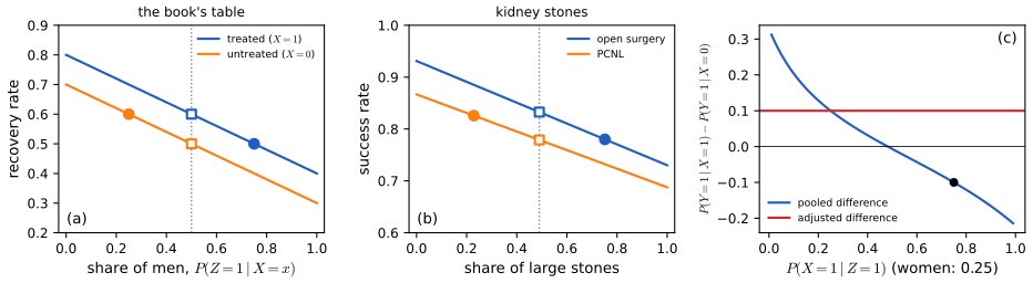
fig_16_s3. Download: PDF · SVGSee also (companion course): the same reversal in a logistic regression, students against non-students at equal credit-card balance, in Applied Statistical Learning in R and Python, Filling the gap 4.3.
pp. 260–261 A real Simpson's paradox, a treatment beneficial for men and for women but harmful overall, cannot happen. If \(\P(C_1=1\given Z=z)>\P(C_0=1\given Z=z)\) for every \(z\), then
\[ \P(C_1=1)=\sum_z\P(C_1=1\given Z=z)\P(Z=z)>\sum_z\P(C_0=1\given Z=z)\P(Z=z)=\P(C_0=1). \]Filling the gap 16.10: the "no paradox" argument needs a pre-treatment \(Z\) pp. 260–261
The argument is complete for a covariate fixed before treatment, such as sex: then \(\P(C_x=1\given Z=z)\) is a well-defined property of the population, and the strict inequality survives averaging because the weights \(\P(Z=z)\) are the same on both sides and are positive for at least one \(z\). The same line shows that the causal effect is the \(\P(Z=z)\)-average of the group effects, \(\th=\sum_z\th_z\P(Z=z)\), so it always lies between the smallest and largest \(\th_z\).
If \(Z\) is affected by the treatment (a mediator, such as blood pressure measured after a drug), \(Z\) itself has potential values \(Z(0),Z(1)\), and "the treatment helps those with \(Z=1\)" has no single meaning: the people with \(Z=1\) under treatment are not the people with \(Z=1\) without it. Then the stratum comparisons are not causal effects, and the pooled comparison is. The same table can arise from both stories. Read \(Z\) in the book's table as a marker measured after a randomised treatment (a biomarker that the treatment raises, say): then \(\P(Z=1\given X=1)=0.75\)
Derivation
For pre-treatment \(Z\), \(\P(C_x=1)\)
16.5 Bibliographic Remarks
p. 261 Potential outcomes as a language for causation are due mainly to Neyman (1923) and Rubin (1974); later developments are due to Robins (1986), Rosenbaum (2002) and others, with a parallel line in econometrics (Heckman, Manski). The book recommends the texts of Pearl (2000), Rosenbaum (2002), Spirtes, Glymour and Scheines (2000) and van der Laan and Robins (2003). For the gaps filled above: Holland (1986) for the "fundamental problem" that only one potential outcome is observed, Manski (1990) for the bounds of Exercise 16.3, Rosenbaum and Rubin (1983) for the propensity score, Horvitz and Thompson (1952) for inverse probability weighting, Angrist and Pischke (2009) for what least squares estimates when effects vary, Simpson (1951) for the paradox, and Imbens and Rubin (2015) and Hernán and Robins (2020) for modern book-length treatments.
Notes on the book
One slip of Chapter 16 is in the author's errata list; the other points are mine, each with the evidence.
Page 257, equation (16.7): the "\(\d z\)" should not be there
The printed formula integrates against \(\d F_Z(z)\,\d z\); the measure is \(\d F_Z(z)\) alone (with a density it would be \(f_Z(z)\,\d z\)). Listed in the author's errata (first list, item 42).
Page 257, Theorem 16.6: a positivity condition is needed
The theorem assumes only (16.6). But \(\E(Y\given X=x,Z=z)\) is undefined on strata where dose \(x\) never occurs, and then \(\th(x)\) is not identified: Filling the gap 16.6 gives two models with the same distribution of the observed \((X,Y,Z)\) and causal effects 1 and 2. The condition \(\P(X=x\given Z=z)>0\) for almost every \(z\) (or a positive conditional density) must be added. Not in the errata lists.
Page 257, Theorem 16.6: "consistent" must mean uniformly (or on average) consistent
The statement "if \(\hr(x,z)\) is a consistent estimate of \(r(x,z)\), then \(\frac1n\sum_i\hr(x,Z_i)\) is consistent for \(\th(x)\)" fails for pointwise consistency. With a continuous \(Z\), take \(\hr_n(x,z)=r(x,z)+n\,\ind\{z\in\{Z_1,\dots,Z_n\}\}\): at any fixed \(z\) it equals \(r(x,z)\) with probability one, so it is consistent at every \(z\), yet \(\frac1n\sum_i\hr_n(x,Z_i)\)
Page 255, conditional causal effects: randomisation must cover \(Z\)
The sentence "in a randomized experiment, \(\th_z=\E(Y\given X=1,Z=z)\)
16.6 Exercises
All five exercises of Chapter 16 (Wasserman, 2004, pp. 261–262), restated in my own words, with complete solutions (hidden).
Exercise 16.1. Construct a population, in the style of Example 16.2, in which \(\alpha>0\) but \(\th<0\).
Solution
We need a treatment that hurts on average but is taken mostly by people who would do well anyway. Take eight people: three survivors \((1,1)\), two anti-responders \((1,0)\) and three doomed \((0,0)\); the survivors take the treatment, the others do not.
\(X\) 1 1 1 0 0 0 0 0 \(Y\) 1 1 1 1 1 0 0 0 \(C_0\) 1* 1* 1* 1 1 0 0 0 \(C_1\) 1 1 1 0* 0* 0* 0* 0* Then \(\th=\frac38-\frac58=-\frac14\): the treatment hurts the two anti-responders and helps nobody. But \(\alpha=\frac33-\frac25=\frac35>0\). In the language of Filling the gap 16.2, \(p_1=3/8\), \(D_1=1-0=1\) and \(D_0=1-\frac25=\frac35\), so \(\alpha-\th\)
\({}=\frac58\cdot1+\frac38\cdot\frac35\) \({}=\frac{17}{20}\), and indeed \(\frac35+\frac14=\frac{17}{20}\). The potential outcomes demo, preset 5, shows this population. Exercise 16.2. Prove Theorem 16.4.
Solution
"In general \(\th(x)\ne r(x)\)": Example 16.5 is a counterexample (\(\th\) constant, \(r\) decreasing); for a continuous dose, the model of Figure 16.S4 gives \(\th(x)=2+0.5x\) against \(r(x)=7.19-0.54x\), where \(r(x)=\E(A\given X=x)+0.5x\) and \(\E(A\given X=x)\)
\({}=2+2\E(Z\given X=x)\) \({}=2-\frac{3}{2.89}(x-5)\) for the jointly Normal \((Z,X)\). "When \(X\) is randomly assigned, \(\th(x)=r(x)\)": for a discrete dose with \(\P(X=x)>0\), \(r(x)\)
\({}=\E(C(X)\given X=x)\) \({}=\E(C(x)\ind\{X=x\})/\P(X=x)\) \({}=\E C(x)\) \({}=\th(x)\) by (16.4) and independence. For a general dose the conditioning event has probability 0, and the substitution lemma of Filling the gap 16.5 gives \(\E(C(X)\given X)=m(X)\) with \(m(x)=\E C(x)\), hence \(r=\th\) almost everywhere with respect to \(F_X\) (everywhere on the support if both are continuous). Exercise 16.3. Data \((X_1,Y_1),\dots,(X_n,Y_n)\) come from an observational study with binary \(X\) and \(Y\). The causal effect \(\th\) cannot be estimated, but it can be bounded. Find lower and upper bounds on \(\th\) that can be estimated consistently, and show that the interval they define has width 1. (Hint: \(\E C_1\)
\({}=\E(C_1\given X=1)\P(X=1)\) \({}+\E(C_1\given X=0)\P(X=0)\).) Solution
In the hint, \(\E(C_1\given X=1)=\E(Y\given X=1)\) is identified, while \(\E(C_1\given X=0)\) concerns the counterfactual outcomes of the untreated and can be anything in \([0,1]\). So
\[ \P(X=1,Y=1)\ \le\ \E C_1\ \le\ \P(X=1,Y=1)+\P(X=0), \] \[ \P(X=0,Y=1)\ \le\ \E C_0\ \le\ \P(X=0,Y=1)+\P(X=1). \]Subtracting the extreme cases,
\[ -\big[\P(X=1,Y=0)+\P(X=0,Y=1)\big]\ \le\ \th\ \le\ \P(X=1,Y=1)+\P(X=0,Y=0). \]The width is the sum of all four cell probabilities, which is 1. The bounds are functions of the cell probabilities of \((X,Y)\), so the sample proportions estimate them consistently (weak law of large numbers and the continuous mapping theorem). They are sharp: setting \(\E(C_1\given X=0)=0\) and \(\E(C_0\given X=1)=1\) (or 1 and 0) is compatible with the data and attains the lower (upper) bound. The interval always contains 0, so without assumptions the data cannot even sign the effect; the confounding-free value \(\alpha\) is one point of it. These are Manski's (1990) bounds. For the population of Filling the gap 16.2 the interval is \([-0.19,0.81]\) under self-selection and \([-0.445,0.555]\) under random assignment; it contains \(\th=0.1\) in both cases, and only randomisation pins \(\th\) down (Figure 16.S5(a)).
Exercise 16.4. Let \(X\in\R\) and \(C_i(x)=\beta_{1i}x\), so each subject has its own slope. Construct a joint distribution of \((\beta_1,X)\) with \(\P(\beta_1>0)=1\) such that \(\E(Y\given X=x)\) is decreasing in \(x\), where \(Y=C(X)\). Interpret.
Solution
Since \(Y=\beta_1X\), \(\E(Y\given X=x)=x\,\E(\beta_1\given X=x)\). It suffices that the subjects who take high doses are the ones who respond least, strongly enough that \(x\E(\beta_1\given X=x)\) decreases. Take \(X\sim\mathrm{Uniform}(1,3)\) and, given \(X=x\), \(\beta_1\sim\mathrm{Gamma}\) with shape 4 and scale \(1/(4x^2)\). Then \(\beta_1>0\) always, \(\E(\beta_1\given X=x)=1/x^2\) and
\[ \E(Y\given X=x)=\frac1x,\qquad\text{decreasing, while}\qquad \th(x)=\E(\beta_1)\,x=\frac x3 \]is increasing (\(\E\beta_1=\frac12\int_1^3x^{-2}\,\d x=\frac13\)). A deterministic version is \(\beta_1=1/X^2\). Interpretation: increasing the dose raises every subject's outcome, yet the observed outcomes fall with the dose, because the dose was chosen in response to the subject's responsiveness (doctors give larger doses to patients who respond poorly: confounding by indication). The regression of \(Y\) on \(X\) answers "what do we see at dose \(x\)?", not "what would a higher dose do?". Simulation with 400 000 subjects reproduces \(\E(Y\given X=x)=1/x\) bin by bin and \(\E\beta_1=1/3\) (Figure 16.S5(b)).
Exercise 16.5. Let \(X\in\{0,1\}\) be randomly assigned, with potential outcomes \((C_0,C_1)\) whose cdfs \(F_0,F_1\) are continuous and strictly increasing, and \(Y=C_X\). Let \(\th=m_1-m_0\) with \(m_x=F_x^{-1}(1/2)\) the median of \(C_x\). Express \(\th\) through the joint distribution of \((X,Y)\) only.
Solution
By randomisation \(X\indep C_x\), and on \(\{X=x\}\), \(Y=C_x\). So for every \(y\), \(\P(Y\le y\given X=x)\)
\[ \th=F_{Y\given X=1}^{-1}(1/2)-F_{Y\given X=0}^{-1}(1/2), \]\({}=\P(C_x\le y\given X=x)\) \({}=\P(C_x\le y)\) \({}=F_x(y)\): the conditional cdf of \(Y\) given \(X=x\) is \(F_x\). Therefore the difference of the medians of \(Y\) in the two arms, estimated consistently by the difference of the sample medians (continuity and strict monotonicity make the population medians unique, which is what sample medians need to converge). Note that \(\th\) is the difference of the medians, not the median of the individual effects \(C_1-C_0\), which depends on the joint law of \((C_0,C_1)\) and is not identified (Filling the gap 16.1(c)). Example: \(C_0\sim\) Exponential(1) and \(C_1=C_0+V^2\) with \(V\sim\N(0.5,1)\) independent: the difference of medians is 1.00 (estimated from the observed arms as 1.00 with 400 000 subjects), while the median of \(C_1-C_0=V^2\) is 0.58.
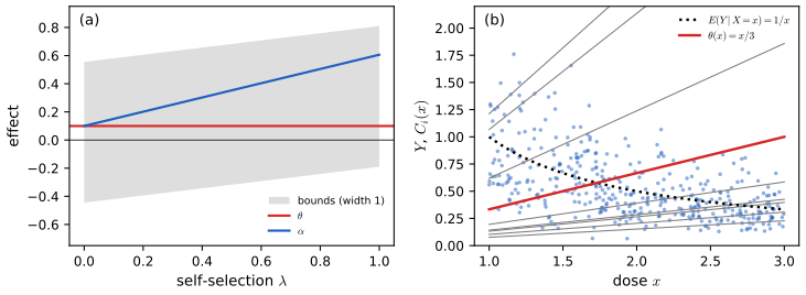
fig_16_s5. Download: PDF · SVGDemonstrations for this chapter
Each demonstration runs in the browser and links back to these notes. The ▶ Demo boxes above open them already set to the case under discussion.
| Demonstration | What you can see | Sections and results |
|---|---|---|
| Potential outcomes | The four response types and who ends up in each arm; \(\th\), \(\alpha\) and the selection bias between them; risk and odds ratios; the path from random assignment to self-selection; the sampling distribution of the difference in means. Presets: 1 Example 16.2; 2 after the advice; 3 a randomised experiment; 4 self-selection; 5 Exercise 16.1. | 16.1; Theorem 16.3; Filling the gaps 16.1–16.3 |
| Adjusting for a confounder | One observational data set by stratum; the limits of the naive, stratified (16.7) and regression (16.8) estimators against the confounding strength; their sampling distributions; empty strata under weak positivity. Presets: 1 no confounding; 2 confounding; 3 a sign reversal; 4 an effect that varies with \(Z\); 5 positivity strain. | 16.3; Theorem 16.6; Filling the gaps 16.6–16.8 |
| Simpson's paradox | Arm rates as weighted averages of group rates; pooled against adjusted differences as the allocation changes; a sampled table; which comparison is causal when \(Z\) comes before or after the treatment. Presets: 1 the book's table; 2 kidney stones; 3 equal allocation; 4 the opposite allocation; 5 \(Z\) caused by the treatment. | 16.4; Filling the gaps 16.9, 16.10 |
Related demonstrations: in the companion courses, the paired design demo of Statistical Methods for Modern Biology (blocking removes variation that randomisation alone leaves in). The Python code that produces every figure of this page is code/ch16_causal_inference.py (see the code index).
References
- Wasserman, L. (2004). All of Statistics: A Concise Course in Statistical Inference. Springer, New York. Chapter 16, pp. 251–262. www.stat.cmu.edu/~larry/all-of-statistics.
- Angrist, J. D. and Pischke, J.-S. (2009). Mostly Harmless Econometrics: An Empiricist's Companion. Princeton University Press, Princeton.
- Charig, C. R., Webb, D. R., Payne, S. R. and Wickham, J. E. A. (1986). Comparison of treatment of renal calculi by open surgery, percutaneous nephrolithotomy, and extracorporeal shockwave lithotripsy. British Medical Journal, 292(6524), 879–882.
- Hernán, M. A. and Robins, J. M. (2020). Causal Inference: What If. Chapman & Hall/CRC, Boca Raton.
- Holland, P. W. (1986). Statistics and causal inference. Journal of the American Statistical Association, 81(396), 945–960.
- Horvitz, D. G. and Thompson, D. J. (1952). A generalization of sampling without replacement from a finite universe. Journal of the American Statistical Association, 47(260), 663–685.
- Imbens, G. W. and Rubin, D. B. (2015). Causal Inference for Statistics, Social, and Biomedical Sciences: An Introduction. Cambridge University Press, Cambridge.
- Julious, S. A. and Mullee, M. A. (1994). Confounding and Simpson's paradox. British Medical Journal, 309(6967), 1480–1481.
- Manski, C. F. (1990). Nonparametric bounds on treatment effects. American Economic Review, 80(2), 319–323.
- Neyman, J. (1923). On the application of probability theory to agricultural experiments. Essay on principles. Section 9. Translated by D. M. Dabrowska and T. P. Speed, Statistical Science, 5(4), 465–472 (1990).
- Pearl, J. (2000). Causality: Models, Reasoning, and Inference. Cambridge University Press, Cambridge.
- Robins, J. M. (1986). A new approach to causal inference in mortality studies with a sustained exposure period: application to control of the healthy worker survivor effect. Mathematical Modelling, 7, 1393–1512.
- Rosenbaum, P. R. (2002). Observational Studies, 2nd edition. Springer, New York.
- Rosenbaum, P. R. and Rubin, D. B. (1983). The central role of the propensity score in observational studies for causal effects. Biometrika, 70(1), 41–55.
- Rubin, D. B. (1974). Estimating causal effects of treatments in randomized and nonrandomized studies. Journal of Educational Psychology, 66(5), 688–701.
- Simpson, E. H. (1951). The interpretation of interaction in contingency tables. Journal of the Royal Statistical Society, Series B, 13(2), 238–241.
- Spirtes, P., Glymour, C. and Scheines, R. (2000). Causation, Prediction, and Search, 2nd edition. MIT Press, Cambridge, MA.
- van der Laan, M. J. and Robins, J. M. (2003). Unified Methods for Censored Longitudinal Data and Causality. Springer, New York.
The numerical statements in the text (the toy populations and their effects, the selection-bias decomposition and the type model, the Fréchet bounds, the standard error and coverage of the randomised comparison, the substitution lemma for a random dose, the dose model and the adjusted estimate (16.8), the limits of the naive, regression and stratified estimators and the regression weights, the equality of weighting and stratification, the Simpson tables and the kidney stone data, and the solutions of the exercises) were confirmed numerically.