Decision Theory
Inference tells us what to believe; decision theory tells us what to do. Given a loss function and a posterior, the best action is the one with the smallest posterior expected loss, and almost every familiar procedure in machine learning (the MAP label, the posterior mean, a probability threshold, the reject option, a choice between models) is a special case. This chapter develops the Bayesian recipe, the evaluation tools built on it (ROC and precision-recall curves, proper scoring rules), Bayesian and information-criterion model selection, the frequentist view of the same problems (risk, minimax, admissibility, empirical risk minimisation, hypothesis tests) and the reasons why the two views can disagree.
Ch. 1 Introduction Ch. 2 Univariate probability Ch. 3 Multivariate probability Ch. 4 Statistics Ch. 5 Decision theory Ch. 6 Information theory Ch. 7 Linear algebra Ch. 8 Optimisation Ch. 9 Discriminant analysis Ch. 10 Logistic regression Ch. 11 Linear regression Ch. 12 GLMs Ch. 13 Networks for tabular data Ch. 14 Networks for images Ch. 15 Networks for sequences Ch. 16 Exemplar-based methods Ch. 17 Kernel methods Ch. 18 Trees and boosting Ch. 19 Fewer labels Ch. 20 Dimensionality reduction Ch. 21 Clustering Ch. 22 Recommender systems Ch. 23 Graph embeddings
How to read these notes
They follow the book. Sections carry the book’s numbers (5.1, 5.1.2, ...) and every displayed equation that restates one of the book’s numbered equations carries the book’s own number, e.g. \((5.34)\). Equations without a number are my own.
Filling the gaps. The book is concise and states many results without proof (“it can be shown”, “one can show”, results quoted from the literature, exercises). Wherever that happens an orange Filling the gap box or a proof gives the full argument. Proofs and derivations start hidden: click a bar to open it, or use the buttons below.
Figures and demonstrations. Every figure of the chapter that is computed from a model or a simulation is reproduced from scratch by the Python code (the cartoon of Figure 5.11 is skipped; the book’s figures use hypothetical systems, so the data here are simulated and say so). The ▶ Demo boxes open an interactive page already set to the case under discussion.
Main reference
K. P. Murphy, Probabilistic Machine Learning: An Introduction, MIT Press (2022), Chapter 5 (book pages 167–205; book web page: probml.github.io/pml-book/book1.html). Section, equation, figure and exercise numbers below refer to the book.
The explanations, derivations, figures and code are my own; equations are cited by their numbers in the book. Where a result goes back to a paper, the paper is cited at the end.
Companion courses
Most of this chapter also appears, with other examples, in two companion courses on this site. The overlapping material is:
- Bayes-optimal actions, the squared, absolute and Huber losses, the reject option, risk, Bayes risk, minimax rules, admissibility and Stein’s paradox: All of Statistics, Chapter 12 (12.3 Bayes estimators, 12.4 minimax rules, 12.6 admissibility, 12.7 Stein’s paradox) and Bayesian and Probabilistic ML, Section 1.5 (decision theory).
- Hypothesis tests, p-values, the Neyman-Pearson lemma, the permutation test and Bayesian testing: All of Statistics, Chapter 10 and Chapter 11, Section 11.8.
- Hoeffding’s inequality and the union bound: All of Statistics, Chapter 4. The bootstrap and cross-validation estimates of risk: Chapter 8.
- The marginal likelihood, the evidence approximation and the Occam factor: Bayesian and Probabilistic ML, Section 3.4 and 3.5; the bias–variance decomposition: Section 3.2. Companion demonstrations: decision theory, the evidence, bias and variance, Bayes rules and losses, base rates.
Where a proof there is identical, these notes state the result, give a short argument and link to it. New here: Murphy’s notation, the ROC and precision-recall analysis (AUC as a probability, the optimal F1 threshold, the effect of prevalence), proper scoring rules, the information criteria (a derivation of BIC and AIC and a correction to the book’s WAIC formula), Bayesian effect-size tests, empirical risk minimisation and Hoeffding’s bound, and the quantitative comparison of p-values with posterior probabilities.
The chapter at a glance
- 5.1.1 The optimal action minimises the posterior expected loss (Result 5.1); this is also what minimises the Bayes risk (Gap 5.1).
- 5.1.2 Zero-one loss gives the MAP label, an asymmetric loss gives the threshold \(1/(1+c)\) (Result 5.2) and a reject cost gives Chow’s rule (Result 5.3).
- 5.1.3–5.1.4 ROC and precision-recall curves show every threshold at once; AUC is the probability that a random positive outranks a random negative (Result 5.4); the ROC curve ignores prevalence, the PR curve and F-scores do not (Gap 5.5).
- 5.1.5–5.1.6 Squared loss gives the mean, absolute loss the median (Result 5.5), log loss and the Brier score are proper scoring rules (Result 5.6).
- 5.2 Bayes factors, the Bayesian Occam razor, the link with cross-validation, BIC, AIC, MDL and WAIC (Gaps 5.12–5.15), and Bayesian tests of effect sizes.
- 5.3 Frequentist risk: the risk functions of Figure 5.8, Bayes risk, minimax, consistency, admissibility and Stein’s paradox (Result 5.9).
- 5.4 Empirical risk minimisation, approximation and estimation error, optimism, cross-validation and Hoeffding’s bound (Result 5.10).
- 5.5 Likelihood ratio tests, the Neyman-Pearson lemma (Result 5.11), p-values, and why a small p-value is not a small posterior probability (Result 5.12).
Notation. \(h\in\mathcal H\) is the state of nature, \(a\in\mathcal A\) an action, \(\ell(h,a)\) the loss, \(\rho(a\given x)=\E[\ell(h,a)\given x]\) the posterior expected loss (risk), \(\pi^*(x)\) the optimal policy. In the frequentist sections \(\theta\) is a fixed parameter, \(\delta\) an estimator and \(R(\theta,\delta)=\E_{x\sim p(\cdot|\theta)}\ell(\theta,\delta(x))\) its risk. \(\Phi\) and \(\varphi\) are the standard normal cdf and density.
5.1 Bayesian decision theory
p. 167 Bayesian inference turns data \(x\) into a posterior \(p(h\given x)\) over the hidden state \(h\). To act we need more: a list of possible actions and a statement of how much each action costs in each state. The Bayesian answer is then mechanical: average the cost over the posterior and pick the action with the smallest average.
See also (companion courses): All of Statistics 12.3, Bayes estimators; Bayesian and Probabilistic ML 1.5, decision theory.
5.1.1 Basics
Definition 5.1 (a decision problem and its Bayes rule) pp. 167–168, (5.1)–(5.3)
A decision problem consists of a set of states of nature \(\mathcal H\), a set of actions \(\mathcal A\) and a loss function \(\ell:\mathcal H\times\mathcal A\to\R\), where \(\ell(h,a)\) is the cost of taking action \(a\) when the state is \(h\). After observing \(x\), the posterior expected loss or risk of action \(a\) is
\[ \rho(a\given x)\triangleq\E_{p(h|x)}[\ell(h,a)]=\sum_{h\in\mathcal H}\ell(h,a)\,p(h\given x), \tag{5.1} \](an integral for continuous \(h\)). The optimal policy, also called the Bayes estimator or Bayes decision rule, is
\[ \pi^*(x)=\delta^*(x)=\argmin_{a\in\mathcal A}\E_{p(h|x)}[\ell(h,a)]. \tag{5.2} \]With a utility \(U(h,a)=-\ell(h,a)\) the same rule is the maximum expected utility principle
\[ \pi^*(x)=\argmax_{a\in\mathcal A}\E_h[U(h,a)]. \tag{5.3} \]The loss is a modelling choice, separate from the probabilistic model: the same posterior leads to different actions under different losses. An agent that only compares expected values is called risk neutral. Risk-averse agents are accommodated by passing the outcome through a concave utility before averaging; this chapter stays risk neutral.
Result 5.1 (optimality of the Bayes rule) (5.2), (5.74)–(5.75)
Let \(\pi_0(\theta)\) be the prior and \(\delta:\mathcal X\to\mathcal A\) any decision rule. If \(\delta^*(x)\) minimises \(\rho(a\given x)\) for every \(x\), then \(\delta^*\) minimises the integrated (Bayes) risk \(R_{\pi_0}(\delta)=\iint\pi_0(\theta)p(x\given\theta)\ell(\theta,\delta(x))\,\d\theta\,\d x\) among all rules, with excess Bayes risk
\[ R_{\pi_0}(\delta)-R_{\pi_0}(\delta^*)=\int p(x)\{\rho(\delta(x)\given x)-\rho(\delta^*(x)\given x)\}\d x\ge0. \]Proof
By Tonelli (the loss is bounded below, say \(\ge0\), after adding a constant) we can integrate over \(\theta\) first: \[R_{\pi_0}(\delta)=\int p(x)\int p(\theta\given x)\ell(\theta,\delta(x))\d\theta\,\d x=\int p(x)\rho(\delta(x)\given x)\d x\], using \(\pi_0(\theta)p(x\given\theta)=p(x)p(\theta\given x)\). The integrand is minimised pointwise in \(x\) by \(\delta^*(x)\), hence so is the integral. ∎
Filling the gap 5.1: case-by-case optimality is optimality on average p. 191, (5.74)–(5.75)
The book states (in Section 5.3.1.2) that picking the best action for each observed \(x\) is optimal on average over data sets, and that “the Bayesian approach provides a good way of achieving frequentist goals”. The content is Result 5.1; three details are worth making explicit.
Derivation
(i) Ties and randomisation. If several actions tie at some \(x\), any choice is Bayes. A randomised rule that picks action \(a\) with probability \(q(a\given x)\) has posterior risk \(\sum_aq(a\given x)\rho(a\given x)\ge\min_a\rho(a\given x)\), so randomisation never helps a Bayesian.
(ii) Existence of the minimiser. For finite \(\mathcal A\) the minimum exists. For continuous actions it exists, for instance, when \(\ell(h,\cdot)\) is convex and coercive; for the squared loss it is the posterior mean (Result 5.5), provided the mean exists.
(iii) What it does not say. The Bayes rule minimises the average over \(\theta\) of the frequentist risk \(R(\theta,\delta)\), not each \(R(\theta,\delta)\); at a particular \(\theta\) another rule can be better (Figure 5.8), and the choice of \(\pi_0\) matters. This is the content of Sections 5.3.1.2 and 5.3.1.3 below.
Now the book’s example. A doctor chooses between “nothing” and an expensive drug with side effects. The state is (age, disease): the age is observed and the disease is inferred from a test. Measuring cost in quality-adjusted life years (QALY), a young patient has 60 years to lose and an old one 10, and the drug costs 8 whatever the state. The loss matrix is
| state | nothing | drug |
|---|---|---|
| no COVID-19, young | 0 | 8 |
| COVID-19, young | 60 | 8 |
| no COVID-19, old | 0 | 8 |
| COVID-19, old | 10 | 8 |
(Table 5.1). Bayes’ rule with prevalence \(0.1\), sensitivity \(0.875\) and specificity \(0.975\) gives \[p(\text{covid}\given\text{positive})=0.0875/0.11=0.795\] and \[p(\text{covid}\given\text{negative})=0.0125/0.89=0.0140\]. The expected cost of doing nothing for each of the four possible observations is (Table 5.2, recomputed by covid_policy):
| test | age | \(p(\text{covid})\) | cost of nothing | cost of the drug | action |
|---|---|---|---|---|---|
| negative | young | 0.014 | 0.84 | 8.00 | nothing |
| negative | old | 0.014 | 0.14 | 8.00 | nothing |
| positive | young | 0.795 | 47.73 | 8.00 | drug |
| positive | old | 0.795 | 7.95 | 8.00 | nothing |
Filling the gap 5.2: thresholds behind Table 5.2, and why 0.80 against 0.81 flips the decision pp. 168–169
The book remarks that cutting the drug cost to 5 treats all positives, and that raising the sensitivity from 0.875 to 0.975 (so \(p\) from 0.80 to 0.81) treats old positives even at cost 8. Why such a small change?
Derivation
With \(p=p(\text{covid}\given x)\) and \(q\) the QALY at stake, the risk of doing nothing is \(pq\) and that of the drug is \(c\) (the drug cost, state independent). So the drug is given iff \(pq\gt c\), that is iff \(p\gt c/q\): the threshold is \(8/60=0.133\) for the young and \(8/10=0.8\) for the old. A positive test gives \(p=0.795\), a hair below the old-age threshold of \(0.8\), which is why the decision is fragile: with sensitivity \(0.975\), \[p=0.0975/(0.0975+0.0225)=0.8125\gt0.8\] and the old positives are treated; with cost 5 the old threshold drops to \(0.5\) and \(p=0.795\) clears it. A negative test (\(p=0.014\)) is below every threshold, so nobody who tests negative is treated. A decision that sits this close to a threshold is a reason to collect more information (a second test) before acting; this is the idea of the value of information in decision theory. All four numbers are confirmed by the code.
5.1.2 Classification problems
p. 169 Take states and actions to be the class labels, \(\mathcal H=\mathcal A=\{1,\dots,C\}\). The loss defines what “best” means.
5.1.2.1 Zero-one loss
Result 5.1b (zero-one loss gives the MAP label) (5.4)–(5.7)
For \(\ell_{01}(y^*,\hat y)=\mathbb I(y^*\ne\hat y)\) the risk is \(\rho(\hat y\given x)=1-p(y^*=\hat y\given x)\) \((5.6)\), so the optimal rule is the mode of the posterior,
\[ \pi(x)=\argmax_{y\in\mathcal Y}p(y\given x). \tag{5.7} \](The proof is the one line above: \(\sum_{y^*}\mathbb I(y^*\ne\hat y)p(y^*\given x)=1-p(\hat y\given x)\).) The Bayes risk of this rule is the Bayes error rate, \(\E_x[1-\max_yp(y\given x)]\), the smallest error any classifier can have.
5.1.2.2 Cost-sensitive classification
Result 5.2 (cost-sensitive threshold) (5.8)–(5.10)
Let \(\ell_{ij}\) be the loss of predicting \(j\) when the truth is \(i\) (so \(\ell_{10}\) is the cost of a false negative and \(\ell_{01}\) of a false positive), \(p_1=p(y^*=1\given x)\), \(p_0=1-p_1\). Label 0 is optimal iff \(\ell_{00}p_0+\ell_{10}p_1\lt\ell_{01}p_0+\ell_{11}p_1\) \((5.9)\), that is, assuming \(\ell_{01}\gt\ell_{00}\) and \(\ell_{10}\gt\ell_{11}\), iff
\[ p_1\lt\frac{\ell_{01}-\ell_{00}}{(\ell_{01}-\ell_{00})+(\ell_{10}-\ell_{11})}. \]With \(\ell_{00}=\ell_{11}=0\) this is \(p_1\lt\ell_{01}/(\ell_{01}+\ell_{10})\) \((5.10)\), and with \(\ell_{10}=c\,\ell_{01}\) (a false negative costs \(c\) times a false positive) the rule is: predict 1 iff \(p_1\ge1/(1+c)\). For \(c=2\) the threshold is \(1/3\).
Proof
Write \(p_0=1-p_1\). Then \(\ell_{00}p_0+\ell_{10}p_1\lt\ell_{01}p_0+\ell_{11}p_1\) is \(\ell_{00}+(\ell_{10}-\ell_{00})p_1\lt\ell_{01}+(\ell_{11}-\ell_{01})p_1\), i.e. \((\ell_{10}-\ell_{00}+\ell_{01}-\ell_{11})p_1\lt\ell_{01}-\ell_{00}\). The coefficient is \((\ell_{01}-\ell_{00})+(\ell_{10}-\ell_{11})\gt0\) under the stated assumptions, which gives the threshold. ∎
The threshold depends on the losses only through the ratio \(c\); it is the same as the cost-based threshold of Section 1.5.2 of the companion course. Note what the rule does not need: it needs a calibrated \(p_1\), and changing the costs changes only the threshold, not the model.
5.1.2.3 Classification with the “reject” option
Result 5.3 (Chow’s rule; Exercise 5.1) (5.11)–(5.15)
Let \(\mathcal A=\{0,1,\dots,C\}\) where \(0\) is “reject”, and \(\ell(y^*,a)=0\) if \(a=y^*\), \(\lambda_r\) if \(a=0\), \(\lambda_e\) otherwise \((5.11)\), with \(0\lt\lambda_r\lt\lambda_e\). Let \(y^*=\argmax_yp(y\given x)\), \(p^*=\max_yp(y\given x)\). The Bayes rule is
\[ a^*=\begin{cases}y^*&\text{if }p^*\gt\lambda^*\\\text{reject}&\text{otherwise}\end{cases},\qquad\lambda^*=1-\frac{\lambda_r}{\lambda_e}. \tag{5.12, 5.15} \]Proof
The risk of answering \(j\) is \(\lambda_e(1-p(j\given x))\), smallest for \(j=y^*\): \(\lambda_e(1-p^*)\). The risk of rejecting is \(\lambda_r\). So answer iff \(\lambda_e(1-p^*)\lt\lambda_r\), i.e. \(p^*\gt1-\lambda_r/\lambda_e\). ∎
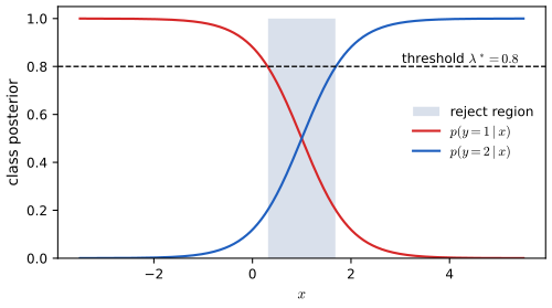
If \(\lambda_r\ge\lambda_e\) then \(\lambda^*\le0\) and rejecting is never optimal. As \(\lambda_r/\lambda_e\) increases from 0 to 1 the threshold falls from 1 to 0 and the reject region (where all posteriors are below \(\lambda^*\)) shrinks to nothing; with \(\lambda_r\to0\) the classifier rejects everything not certain. Figure 5.1 shows the reject region for two overlapping classes.
5.1.3 ROC curves
p. 171 Section 5.1.2.2 shows that the right threshold \(\tau\) depends on costs that may be unknown, differ between users, or change over time. An ROC curve displays the performance for all thresholds at once.
5.1.3.1 Class confusion matrices
For the rule \(\hat y_\tau(x)=\mathbb I(p(y=1\given x)\ge1-\tau)\) \((5.16)\) on \(N\) labelled examples, \(\mathrm{TP}\), \(\mathrm{FP}\), \(\mathrm{TN}\), \(\mathrm{FN}\) count the cells of the confusion matrix \(\mathbf C\), \(C_{ij}\) = number of items of true class \(i\) labelled \(j\) (Table 5.3). Normalising by rows gives \(p(\hat y\given y)\): the true positive rate (sensitivity, recall) and false positive rate
\[ \mathrm{TPR}_\tau=p(\hat y=1\given y=1,\tau)=\frac{\mathrm{TP}_\tau}{\mathrm{TP}_\tau+\mathrm{FN}_\tau},\qquad\mathrm{FPR}_\tau=p(\hat y=1\given y=0,\tau)=\frac{\mathrm{FP}_\tau}{\mathrm{FP}_\tau+\mathrm{TN}_\tau}. \tag{5.18, 5.19} \]with \(\mathrm{FNR}=1-\mathrm{TPR}\) (miss rate, type II error) and \(\mathrm{TNR}=1-\mathrm{FPR}\) (specificity); the type I error is the FPR (Table 5.4). Normalising by columns gives \(p(y\given\hat y)\): the precision (positive predictive value) \(\mathrm{TP}/(\mathrm{TP}+\mathrm{FP})\), the false discovery rate \(1-\)precision, and the negative predictive value and false omission rate (Table 5.5). The two normalisations answer different questions: row rates describe the classifier (how it treats each class), column rates describe the alarm (how much to trust a positive or a negative output), and the latter depend on the prevalence.
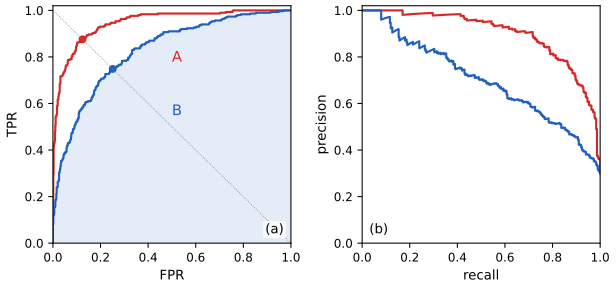
Plotting TPR against FPR as \(\tau\) varies traces the ROC curve (receiver operating characteristic, Figure 5.2a).
5.1.3.2 Summarizing ROC curves as a scalar
The area under the curve (AUC) is the usual scalar, with maximum 1; the equal error rate (EER) is the value at which \(\mathrm{FPR}=\mathrm{FNR}\), found where the curve crosses the anti-diagonal (lower is better, minimum 0).
Result 5.4 (AUC is a probability; ROC curves are invariant) Section 5.1.3.2; Exercise 5.3
Let \(S\) be the score of a classifier, \(S_1\) the score of a random positive and \(S_0\) of an independent random negative, with distribution functions \(F_1,F_0\). Then (a) \(\mathrm{AUC}=\Pr(S_1\gt S_0)+\tfrac12\Pr(S_1=S_0)\); for continuous scores \(\mathrm{AUC}=\Pr(S_1\gt S_0)\). (b) The ROC curve is unchanged by any strictly increasing transformation of the score and by any change of the class proportions. (c) For binormal scores \(S_0\sim\N(0,1)\), \(S_1\sim\N(d,1)\) the ROC curve is \(\mathrm{TPR}=\Phi(d-\Phi^{-1}(1-\mathrm{FPR}))\) and \(\mathrm{AUC}=\Phi(d/\sqrt2)\).
Proof
(a) With threshold \(t\), \(\mathrm{FPR}(t)=\Pr(S_0\gt t)=1-F_0(t)\) and \(\mathrm{TPR}(t)=1-F_1(t)\). For continuous scores, parametrise the curve by \(u=\mathrm{FPR}(t)\), \(t=t(u)\) decreasing in \(u\): \[\mathrm{AUC}=\int_0^1\mathrm{TPR}\,\d u=\int\Pr(S_1\gt t)\,\d(\mathrm{FPR})\]. Since \(-\d\,\mathrm{FPR}(t)=f_0(t)\d t\), \[\mathrm{AUC}=\int\Pr(S_1\gt t)f_0(t)\d t=\Pr(S_1\gt S_0)\]. With ties the empirical curve joins the tied points by a straight segment, which adds half the tied mass, giving the second term. (b) A strictly increasing \(g\) maps the set \(\{S\ge t\}\) to \(\{g(S)\ge g(t)\}\): the family of predicted-positive sets, hence the set of attainable \((\mathrm{FPR},\mathrm{TPR})\) pairs, is the same. The rates are conditional on the class, so the class proportions do not enter. (c) \(\mathrm{FPR}=1-\Phi(t)\) gives \(t=\Phi^{-1}(1-\mathrm{FPR})\) and \(\mathrm{TPR}=1-\Phi(t-d)=\Phi(d-t)\). And \(S_1-S_0\sim\N(d,2)\), so \(\Pr(S_1\gt S_0)=\Phi(d/\sqrt2)\). ∎
Filling the gap 5.3: Bayes factor against posterior (Exercise 5.3), and which score gives the best ROC pp. 171–173, p. 205
The ROC curve of the posterior \(p(H_1\given D)\) and of the Bayes factor \(B=p(D\given H_1)/p(D\given H_0)\) are identical, and both are the best possible.
Derivation
Same ROC. By Bayes’ rule the posterior odds are the prior odds times \(B\): \(p(H_1\given D)=\pi_1B/(\pi_1B+\pi_0)\), a strictly increasing function of \(B\) for fixed priors \(\pi_0,\pi_1\). By Result 5.4(b) the two scores have the same ROC curve. (The priors affect only which point on the curve a given posterior threshold corresponds to.)
Optimality (Neyman-Pearson, Result 5.11). Among all scores, the likelihood ratio has the highest TPR at every FPR: thresholding \(B\) is the most powerful test of its size. Consequently the ROC curve of the true likelihood ratio dominates every other classifier’s curve and is concave (a mixture of two thresholds is a randomised classifier that attains the chord; the best curve cannot lie below the chord). The AUC of any score is therefore at most that of the likelihood ratio. Numerically (code): the AUC of the posterior and of the Bayes factor coincide to machine precision, and equal that of the raw binormal score.
5.1.3.3 Class imbalance
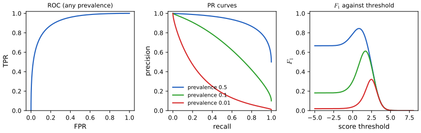
The ROC curve does not change with the prevalence (Result 5.4(b)), but its usefulness can: when negatives vastly outnumber positives a large change in the number of false alarms barely moves the FPR (the denominator is huge), so all the interesting action is squeezed into the extreme left of the plot. Precision-recall curves (next section) fix this by replacing the FPR with the precision.
5.1.4 Precision-recall curves
p. 174 Sometimes the number of true negatives is not part of the problem: an object detector examines a number of image patches that is a tuning parameter, and a retrieval system chooses how many candidates to rank. Then the FPR is not meaningful, and one works with quantities computed from the predicted positives and the true positives only.
5.1.4.1 Computing precision and recall
\[ P(\tau)\triangleq p(y=1\given\hat y=1,\tau)=\frac{\mathrm{TP}_\tau}{\mathrm{TP}_\tau+\mathrm{FP}_\tau},\qquad R(\tau)\triangleq p(\hat y=1\given y=1,\tau)=\frac{\mathrm{TP}_\tau}{\mathrm{TP}_\tau+\mathrm{FN}_\tau}, \tag{5.20, 5.21} \]and in terms of labels \(y_n\) and predictions \(\hat y_n\in\{0,1\}\): \(P=\sum_ny_n\hat y_n/\sum_n\hat y_n\), \(R=\sum_ny_n\hat y_n/\sum_ny_n\) \((5.22, 5.23)\). Recall is the TPR. The precision-recall curve plots \(P\) against \(R\) as \(\tau\) varies (Figure 5.2b); the best classifiers hug the top right corner.
5.1.4.2 Summarizing PR curves as a scalar
The precision at \(K\) is the precision of the top \(K\) ranked items. The raw curve can zigzag (precision may rise with recall when a new true positive arrives), so one uses the interpolated precision \(P_{\rm int}(r)=\max_{r'\ge r}P(r')\), the best precision achievable at recall at least \(r\); the average precision (AP) is the average of the interpolated precision over recall, i.e. the area under the interpolated curve; the mean average precision (mAP) averages AP over several curves (queries or classes).
Filling the gap 5.4: why the interpolated precision is the right envelope, and AP as an integral pp. 174–175
The book says AP equals the area under the interpolated PR curve and may differ from the area under the raw one, without saying why.
Derivation
Sort items by decreasing score and let \(k\) index the thresholds, with \(\mathrm{TP}_k\) true positives among the top \(k\) and \(P\) positives overall. Recall \(R_k=\mathrm{TP}_k/P\) only changes at ranks where the \(k\)-th item is positive, jumping by \(1/P\); precision \(P_k=\mathrm{TP}_k/k\) falls between jumps (the denominator grows, the numerator does not) and rises at a jump (both grow, and \(\mathrm{TP}_k/k\) increases when the added item is positive and \(P_{k-1}\lt1\)). Hence the raw curve is a saw-tooth. A user who needs recall at least \(r\) can use any threshold with \(R_k\ge r\), so the best available precision is \(\max_{k:R_k\ge r}P_k\), the interpolated precision, a non-increasing step function of \(r\). Then \[ \mathrm{AP}=\sum_{j=1}^{P}\frac1P\,P_{\rm int}\!\left(\tfrac jP\right)=\int_0^1P_{\rm int}(r)\,\d r,\] the average over the \(P\) recall levels at which the curve has a jump, which equals the area under the (piecewise constant) interpolated curve. The raw curve lies below its interpolation everywhere, so its trapezoid area is smaller or equal; the two coincide when the precision is monotone. Numerically (code): for system A of Figure 5.2 the interpolated AP is within 0.02 of the step-function AP of scikit-learn, which uses the same idea without the extra maximum.
5.1.4.3 F-scores
At a fixed threshold the pair \((P,R)\) is combined into one number, the \(F_\beta\) score, a weighted harmonic mean of precision and recall:
\[ \frac1{F_\beta}=\frac1{1+\beta^2}\frac1P+\frac{\beta^2}{1+\beta^2}\frac1R,\tag{5.24} \] \[ F_\beta=(1+\beta^2)\frac{PR}{\beta^2P+R}=\frac{(1+\beta^2)\mathrm{TP}}{(1+\beta^2)\mathrm{TP}+\beta^2\mathrm{FN}+\mathrm{FP}}.\tag{5.25} \]For \(\beta=1\): \[F_1=2PR/(P+R)=\mathrm{TP}/(\mathrm{TP}+\tfrac12(\mathrm{FP}+\mathrm{FN}))\] \((5.26, 5.27)\). Larger \(\beta\) weights recall more, \(\beta=2\) for recall-critical tasks and \(\beta=0.5\) for precision-critical ones.
Filling the gap 5.5: the F-score identities, the harmonic mean, class imbalance, and the optimal F1 threshold pp. 175–176, (5.24)–(5.31)
The book gives (5.24)–(5.31) with the intermediate steps left out and states the effect of prevalence only in words. Here are the algebra, the harmonic-mean argument, and a result the book does not give: where the best \(F_1\) threshold is.
Derivation
(5.24) to (5.25). Insert \(1/P=(\mathrm{TP}+\mathrm{FP})/\mathrm{TP}\) and \(1/R=(\mathrm{TP}+\mathrm{FN})/\mathrm{TP}\): \[\frac1{F_\beta}=\frac{(\mathrm{TP}+\mathrm{FP})+\beta^2(\mathrm{TP}+\mathrm{FN})}{(1+\beta^2)\mathrm{TP}}=\frac{(1+\beta^2)\mathrm{TP}+\beta^2\mathrm{FN}+\mathrm{FP}}{(1+\beta^2)\mathrm{TP}},\] which is the second form of (5.25); and \((1+\beta^2)PR/(\beta^2P+R)\) is the same expression after multiplying numerator and denominator of (5.24)’s inverse by \(PR\). Dividing numerator and denominator of the \(\beta=1\) case by 2 gives (5.27).
Harmonic against arithmetic mean. The harmonic mean of positive numbers is at most their arithmetic mean and is dominated by the smaller one: \(2PR/(P+R)\le2\min(P,R)\). The book’s example, predict everything positive at prevalence \(10^{-4}\): \(R=1\), \(P=10^{-4}\), arithmetic mean \(\approx0.5\), \(F_1=2\cdot10^{-4}/(1+10^{-4})\approx0.02\%\). Only a classifier with both high precision and high recall scores well.
Precision and \(F_\beta\) from the rates (5.28)–(5.31). Let \(P_+\) and \(N_-\) be the numbers of positives and negatives and \(r=P_+/N_-=\pi/(1-\pi)\). Then \(\mathrm{TP}=P_+\mathrm{TPR}\), \(\mathrm{FP}=N_-\mathrm{FPR}\), so \[\mathrm{Prec}=\frac{P_+\mathrm{TPR}}{P_+\mathrm{TPR}+N_-\mathrm{FPR}}=\frac{\mathrm{TPR}}{\mathrm{TPR}+\mathrm{FPR}/r}\tag{5.28}\] and, using \(\mathrm{FN}=P_+(1-\mathrm{TPR})\) in (5.25), \[F_\beta=(1+\beta^2)\mathrm{TPR}\big/\big(\mathrm{TPR}+\mathrm{FPR}/r+\beta^2\big)\] \((5.31)\). For a fixed ROC point, precision and \(F_\beta\) are increasing in \(r\): \(\mathrm{Prec}\to1\) as \(r\to\infty\) and \(\to0\) as \(r\to0\). Moving from \(r=0.5\) to \(r=0.1\) lowers the precision at every threshold while the recall (TPR) is unchanged, so the PR curve drops (Figure 5.S1, demo preset 2).
The best \(F_1\) threshold is half the best \(F_1\). Suppose the classifier is calibrated, \(p_i=p(y_i=1\given x_i)\), and predict positive for the top \(k\) items by \(p_i\). The expected counts satisfy \(\mathrm{TP}=A_k=\sum_{i\le k}p_i\) and \(\mathrm{FP}+\mathrm{FN}=k-A_k+(P_+-A_k)\), so \(F_1=2A_k/(k+P_+)\). Adding item \(k+1\) changes \(F_1\) from \(2A_k/(k+P_+)\) to \(2(A_k+p)/(k+1+P_+)\), and \[ \frac{A_k+p}{k+1+P_+}\gt\frac{A_k}{k+P_+}\iff p\,(k+P_+)\gt A_k\iff p\gt\frac{A_k}{k+P_+}=\frac{F_1^{(k)}}2. \] So items should be added as long as their probability exceeds half the current \(F_1\); at the optimum \(k^*\) the threshold on \(p\) equals \(F_1^*/2\) (up to the discreteness of the items). This is why the \(F_1\)-optimal threshold is typically far below 0.5, and why it depends on the prevalence. The code confirms \(\tau^*=F_1^*/2\) for a binormal model with prevalence 0.2 to three decimals.
5.1.5 Regression problems
p. 176 Now actions and states are real numbers, \(\mathcal A=\mathcal H=\R\) (apply the loss element-wise for vectors).
Result 5.5 (squared loss gives the mean, absolute loss the median; Exercise 5.4) (5.32)–(5.36)
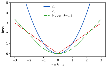
(a) For \(\ell_2(h,a)=(h-a)^2\) the risk is \(\rho(a\given x)=\E[h^2\given x]-2a\E[h\given x]+a^2\) \((5.33)\), uniquely minimised by the posterior mean \(\pi(x)=\E[h\given x]\) \((5.34)\) (the minimum mean squared error, MMSE, estimate), with minimum risk \(\var[h\given x]\). (b) For \(\ell_1(h,a)=|h-a|\) \((5.35)\), every posterior median \(m\) (a value with \(\Pr(h\le m\given x)\ge\tfrac12\) and \(\Pr(h\ge m\given x)\ge\tfrac12\)) is optimal, and only medians are. (c) The Huber loss
\[ \ell_\delta(h,a)=\begin{cases}r^2/2&|r|\le\delta\\\delta|r|-\delta^2/2&|r|\gt\delta\end{cases},\quad r=h-a, \tag{5.36} \]is convex and continuously differentiable, equal to \(\ell_2/2\) for small errors and linear for large ones; the optimal action solves \(\E[\psi_\delta(h-a)\given x]=0\) with \(\psi_\delta(r)=\max(-\delta,\min(r,\delta))\) (the clipped residual).
Proof
(a) \(\rho(a)=(a-\E h)^2+\var h\) after completing the square; the derivative condition \((5.34)\) is \(-2\E h+2a=0\). (b) (Exercise 5.4.) Let \(m\) be a median and \(a\gt m\). Put \(g(h)=|h-a|-|h-m|\). For \(h\le m\), \(g=a-m\); for \(h\ge a\), \(g=-(a-m)\); for \(m\lt h\lt a\), \(g=a+m-2h\gt-(a-m)\). So \(g(h)\ge(a-m)\{\mathbb I(h\le m)-\mathbb I(h\gt m)\}\), and taking expectations, \[\rho(a)-\rho(m)\ge(a-m)\{\Pr(h\le m)-\Pr(h\gt m)\}=(a-m)(2\Pr(h\le m)-1)\ge0\]. For \(a\lt m\) the mirror argument uses \(\Pr(h\ge m)\ge\frac12\). Strictness: if \(a\) is not a median then one of the two half-line probabilities is below \(\tfrac12\) and the inequality is strict (apply the argument with a median \(m\) on the other side of \(a\)). (c) \(\ell_\delta\) is the Moreau-type smoothing of \(|r|\): \(\ell_\delta'(r)=\psi_\delta(r)\) is continuous, non-decreasing, so \(\ell_\delta\) is convex and \(C^1\); the first-order condition \(\frac{\d}{\d a}\E\ell_\delta(h-a)=-\E\psi_\delta(h-a)=0\) is necessary and sufficient. ∎
Filling the gap 5.6: mean, median and the Huber estimator on a skewed posterior; robust regression pp. 176–177
For a symmetric posterior the three estimates coincide; for a skewed or heavy-tailed one they differ, and that is the point of choosing the loss.
Derivation
Take a posterior sample \(h=z^2+\tfrac12\epsilon\), \(z,\epsilon\sim\N(0,1)\) (right skewed). The mean is \(1\), the median about \(0.61\) and the Huber minimiser with \(\delta=1.5\) (about \(0.78\)) lies in between, because it behaves like the mean for the bulk of the sample and like the median in the right tail: \(\E\psi_\delta(h-a)=0\) says the clipped residuals balance. The code minimises each risk on a grid and finds the mean and the median to three decimals. As \(\delta\to\infty\) the Huber minimiser tends to the mean, as \(\delta\to0\) to the median. Using \(\ell_1\) or Huber as a regression loss turns a non-robust least-squares fit into a robust one (Sections 11.6.1 and 11.6.3 of the book): by the same first-order condition the fitted line balances clipped residuals, so a far outlier has bounded influence \(\psi_\delta\le\delta\), where least squares has influence proportional to the residual.
5.1.6 Probabilistic prediction problems
p. 177 Now the action is a whole predictive distribution \(a=q(Y\given x)\) and the state is the true conditional \(h=p(Y\given x)\) (dropped from the notation below). The question is which loss encourages honest forecasts.
5.1.6.1 KL, cross-entropy and log-loss
The Kullback-Leibler divergence, entropy and cross-entropy are
\[ D_{\mathrm{KL}}(p\|q)=\sum_yp(y)\log\frac{p(y)}{q(y)}\ \ (5.37),\qquad H(p)=-\sum_yp(y)\log p(y),\quad H_{ce}(p,q)=-\sum_yp(y)\log q(y), \] \[ D_{\mathrm{KL}}(p\|q)=-H(p)+H_{ce}(p,q).\tag{5.38, 5.39} \]\(D_{\rm KL}\ge0\) with equality iff \(p=q\) (proved below and again in Chapter 6). Since \(H(p)\) does not depend on \(q\), minimising the KL over \(q\) is minimising the cross-entropy, \(q^*=\argmin_qH_{ce}(p,q)\) \((5.42)\). If the truth is one-hot, \(p=\mathbb I(Y=c)\), the cross-entropy is the log loss \(-\log q(c)\) \((5.43)\). In coding terms \(H(p)\) is the minimal expected code length for data from \(p\), \(H_{ce}(p,q)\) the length when the code is built for \(q\), and the KL the excess.
5.1.6.2 Proper scoring rules
Result 5.6 (the log score and the Brier score are strictly proper) Sections 5.1.6.2–5.1.6.3, (5.44)
A loss \(\ell(p,q)\) between a true distribution \(p\) and a reported distribution \(q\) is a proper scoring rule if \(\ell(p,p)\le\ell(p,q)\) for all \(q\), and strictly proper if equality holds only for \(q=p\). (a) The cross-entropy \(H_{ce}(p,q)\) is strictly proper. (b) The Brier score, for a forecast vector \(q\) and a one-hot outcome \(e_Y\) with \(Y\sim p\), has expected value \(\E_p\|q-e_Y\|^2=\|q-p\|^2+1-\|p\|^2\), so it is strictly proper.
Proof
(a) \(H_{ce}(p,q)-H_{ce}(p,p)=D_{\rm KL}(p\|q)\ge0\). To prove the inequality, let \(S=\{y:p(y)\gt0\}\) and use \(\log t\le t-1\) (equality only at \(t=1\)): \[-D_{\rm KL}(p\|q)=\sum_{y\in S}p(y)\log\frac{q(y)}{p(y)}\le\sum_{y\in S}p(y)\big(\frac{q(y)}{p(y)}-1\big)=\sum_{y\in S}q(y)-1\le0\]. Equality forces \(q(y)=p(y)\) on \(S\) and \(q=0\) off \(S\). (b) \[\E_p\|q-e_Y\|^2=\|q\|^2-2\sum_yq(y)p(y)+1=\|q-p\|^2-\|p\|^2+1\]. It is minimised, uniquely, at \(q=p\), where it equals \(1-\|p\|^2\). ∎
5.1.6.3 Brier score
For \(N\) forecasts \(q_n\) of outcomes \(y_n\) in one-hot form,
\[ \mathrm{BS}=\frac1N\sum_{n=1}^N\sum_{c=1}^C(q_{nc}-y_{nc})^2,\tag{5.44} \]the mean squared error of the forecast vectors. The Brier skill score \(\mathrm{BSS}=1-\mathrm{BS}/\mathrm{BS}_{\rm ref}\) compares with a reference forecast, often the in-sample frequency (“climatology”); 1 is perfect, 0 is no better than the reference.
Filling the gap 5.7: binary Brier score, boundedness, and the decomposition p. 179
Derivation
For two classes with \(y_n=y_{n1}\), \(q_n=q_{n1}\): \[(q_n-y_n)^2+\{(1-q_n)-(1-y_n)\}^2=2(q_n-y_n)^2\], so the multi-class score is twice the binary one \(\frac1N\sum(q_n-y_n)^2\in[0,1]\) (checked numerically in the code). The log loss is unbounded (\(-\log q(c)\to\infty\) as the probability given to the true class tends to 0), so one confidently wrong forecast can dominate the average; the Brier score of one forecast is at most 2 (at most 1 in the binary form). This is the sense in which it is less sensitive to very rare events. If \(q_n\) takes \(K\) distinct values \(v_k\) over \(N_k\) cases with observed frequency \(\bar y_k\), then the binary score \[\mathrm{BS}=\frac1N\sum_kN_k(v_k-\bar y_k)^2+\bar y(1-\bar y)-\frac1N\sum_kN_k(\bar y_k-\bar y)^2\]: calibration (reliability) minus resolution plus uncertainty (Murphy, 1973), because the within-group variance of a 0/1 variable with frequency \(\bar y_k\) is \(\bar y_k(1-\bar y_k)\).
5.2 Choosing the “right” model
p. 179 Suppose several candidate models (networks with different depths, polynomials of different degrees) are available and we must choose one. This is a decision problem like any other: the actions are the models, and the states are which model is true.
See also (companion course): Section 3.4, Bayesian model comparison, 3.5, the evidence approximation; evidence demo.
5.2.1 Bayesian hypothesis testing
With two models, the null \(M_0\) and the alternative \(M_1\), and zero-one loss (Result 5.1b), the Bayes rule picks \(M_1\) iff \(p(M_1\given D)\gt p(M_0\given D)\). With equal priors this is a comparison of marginal likelihoods, whose ratio is the Bayes factor
\[ B_{1,0}\triangleq\frac{p(D\given M_1)}{p(D\given M_0)}.\tag{5.45} \]It is a likelihood ratio in which the parameters have been integrated out against the prior rather than maximised, which lets it compare models of different complexity (Section 5.2.3). With a general prior and losses \(L_{ij}\) (cost of choosing \(M_j\) when \(M_i\) is true) the rule is again a threshold: choose \(M_1\) iff \(B_{1,0}\gt\frac{p(M_0)(L_{01}-L_{00})}{p(M_1)(L_{10}-L_{11})}\), by Result 5.2 applied to the posterior \(p(M_1\given D)=\frac{p(M_1)B_{1,0}}{p(M_1)B_{1,0}+p(M_0)}\). Jeffreys (1961) suggested reading the size of \(B\) on a verbal scale (Table 5.6): below \(1/100\) is decisive evidence for \(M_0\), \(1/100\) to \(1/10\) strong, \(1/10\) to \(1/3\) moderate, \(1/3\) to \(1\) weak; and symmetrically above 1 (weak up to 3, moderate to 10, strong to 100, decisive beyond). It is a Bayesian counterpart of the p-value, with a very different meaning (Section 5.5.4).
5.2.1.1 Example: testing if a coin is fair
\(M_0\): \(\theta=\frac12\), so \(p(D\given M_0)=(\frac12)^N\) \((5.46)\). \(M_1\): \(\theta\sim\mathrm{Beta}(\alpha_1,\alpha_0)\), so by the Beta integral \((4.143)\)
\[ p(D\given M_1)=\int p(D\given\theta)p(\theta)\d\theta=\frac{B(\alpha_1+N_1,\alpha_0+N_0)}{B(\alpha_1,\alpha_0)}.\tag{5.47} \]Filling the gap 5.8: the coin Bayes factor in closed form, and when the fair coin wins (Figure 5.4) pp. 180–181
Derivation
(5.47). For a particular sequence with \(N_1\) heads and \(N_0\) tails, \(p(D\given\theta)=\theta^{N_1}(1-\theta)^{N_0}\) and \(p(\theta)=\theta^{\alpha_1-1}(1-\theta)^{\alpha_0-1}/B(\alpha_1,\alpha_0)\). Their product integrates to \(B(\alpha_1+N_1,\alpha_0+N_0)/B(\alpha_1,\alpha_0)\) by the definition \(B(a,b)=\int_0^1t^{a-1}(1-t)^{b-1}\d t\). If instead we record only the count \(N_1\), both marginal likelihoods gain the same factor \(\binom N{N_1}\), which cancels in \(B\).
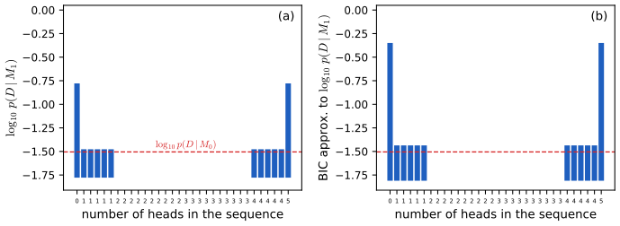
Uniform prior. With \(\alpha_1=\alpha_0=1\), \(B(1+N_1,1+N_0)=N_1!N_0!/(N+1)!\), so \[ B_{0,1}=\frac{p(D\given M_0)}{p(D\given M_1)}=\frac{(N+1)!}{2^NN_1!N_0!}=(N+1)\binom N{N_1}2^{-N}=(N+1)\,\mathrm{Bin}\!\left(N_1;N,\tfrac12\right). \] The fair coin is preferred iff \((N+1)\mathrm{Bin}(N_1;N,\frac12)\gt1\), i.e. when the head count is near \(N/2\) so that the binomial probability exceeds \(1/(N+1)\), which is the average probability of a count under the free coin. For \(N=5\): \(N_1=2,3\) give \(6\cdot10/32=1.875\) (fair coin favoured), \(N_1=1,4\) give \(6\cdot5/32=0.94\) and \(N_1=0,5\) give \(6/32=0.19\) (free coin favoured). The intuition is as in the book: a free coin could have produced almost any sequence, so it spreads its probability thinly; an almost balanced sequence would be a suspicious coincidence if the coin were biased. Because \(\log p(D\given M_0)\) is a constant, the log Bayes factor has exactly the shape of Figure 5.4a.
5.2.2 Bayesian model selection
For a set \(\mathcal M\) of models, with zero-one loss the Bayes rule is the MAP model
\[ \hat m=\argmax_{m\in\mathcal M}p(m\given D),\qquad p(m\given D)=\frac{p(D\given m)p(m)}{\sum_{m'}p(D\given m')p(m')},\tag{5.48, 5.49} \]and for a uniform prior \(\hat m=\argmax_mp(D\given m)\) \((5.50)\), where the marginal likelihood or evidence is \(p(D\given m)=\int p(D\given\theta,m)p(\theta\given m)\d\theta\) \((5.51)\).
5.2.2.1 Example: polynomial regression
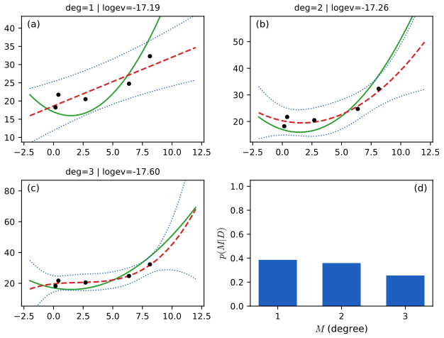
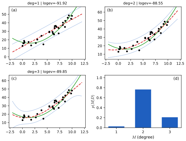
Figures 5.5 and 5.6 compare polynomials of degree 1, 2 and 3 fitted to \(N=5\) and \(N=30\) points with a uniform prior over the degrees and an empirical-Bayes prior on the weights.
Filling the gap 5.9: the evidence of Bayesian polynomial regression and empirical Bayes pp. 181–183 (details in Section 11.7)
The book refers to Section 11.7 for the computation. Here is the formula used by the code.
Derivation
Model of degree \(m\): \(y=\Phi\mathbf w+\boldsymbol\epsilon\) with \(\Phi_{nj}=u_n^{j}\), \(j=0,\dots,m\) (here \(u=(x-5)/5\)), prior \(\mathbf w\sim\N(\mathbf 0,\alpha^{-1}\mathbf I)\) and noise \(\boldsymbol\epsilon\sim\N(\mathbf0,\beta^{-1}\mathbf I)\). The vector \(\mathbf y\) is an affine function of the jointly Gaussian \((\mathbf w,\boldsymbol\epsilon)\), hence Gaussian with mean \(\mathbf0\) and covariance \(\beta^{-1}\mathbf I+\alpha^{-1}\Phi\Phi^\T\). Therefore \[ \log p(\mathbf y\given\alpha,\beta,m)=-\tfrac12\big\{N\log2\pi+\log\det\mathbf C+\mathbf y^\T\mathbf C^{-1}\mathbf y\big\},\qquad\mathbf C=\beta^{-1}\mathbf I+\alpha^{-1}\Phi\Phi^\T. \] This is the evidence if \(\alpha,\beta\) are fixed. Empirical Bayes maximises it over \((\alpha,\beta)\) for each \(m\) (type-II maximum likelihood; the code uses L-BFGS on \((\log\alpha,\log\beta)\) from nine starting points), and \(p(m\given D)\propto p(D\given\hat\alpha_m,\hat\beta_m,m)\) for the uniform prior over \(m\in\{1,2,3\}\). The predictive distribution at \(u\) is \(\N(\mathbf m_N^\T\boldsymbol\phi(u),\beta^{-1}+\boldsymbol\phi(u)^\T\mathbf S_N\boldsymbol\phi(u))\) with \(\mathbf S_N=(\alpha\mathbf I+\beta\Phi^\T\Phi)^{-1}\), \(\mathbf m_N=\beta\mathbf S_N\Phi^\T\mathbf y\), which gives the \(\pm2\sigma\) bands. The same formula is derived in Section 3.5.1 of the companion course, with the fixed-point updates for \(\alpha,\beta\). Caveat. With only 5 points the posterior over degrees is not sharp; the plotted data set was drawn with a fixed seed. Over 60 seeds the MAP degree for \(N=5\) was 1 in 32, 2 in 19 and 3 in 9 data sets; for \(N=30\) it was 2 in 58 of 60 (3 in the other two), so the second figure is typical and the first shows the tendency of small samples to favour the simpler model without being a certainty.
5.2.3 Occam’s razor
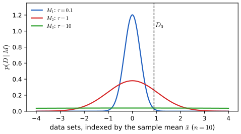
If a simple model \(m_1\) and a complex model \(m_2\) both fit the data well at their best parameters, we prefer \(m_1\). The marginal likelihood implements this automatically for two linked reasons. (i) The prior of the complex model is spread over a larger parameter volume, so averaging the likelihood against it takes in many poor parameter values. (ii) Since \(\sum_{D'}p(D'\given m)=1\), a model that can predict many data sets must give each a small probability (conservation of probability mass, Figure 5.7).
Filling the gap 5.10: the Occam factor and conservation of probability mass, made quantitative pp. 183–184
Derivation
Conservation. \[\sum_{D'}p(D'\given m)=\sum_{D'}\int p(D'\given\theta,m)p(\theta\given m)\d\theta=\int p(\theta\given m)\sum_{D'}p(D'\given\theta,m)\d\theta=1\]. The same holds with integrals over data sets (check: the three marginal densities of Figure 5.7 each integrate to one).
Occam factor. If the likelihood \(p(D\given\theta,m)\) is sharply peaked around \(\hat\theta\) with width \(\sigma_{\rm post}\) (the posterior width) and the prior is roughly flat with width \(\sigma_{\rm prior}\), then \[ p(D\given m)\approx p(D\given\hat\theta,m)\times\frac{\sigma_{\rm post}}{\sigma_{\rm prior}}, \] a best-fit likelihood times the Occam factor \(\sigma_{\rm post}/\sigma_{\rm prior}\le1\), the fraction of the prior volume that survives the data. A model with more parameters has one such factor per parameter, hence a smaller evidence at the same best fit. Exact example (Figure 5.7). Data \(x_1,\dots,x_n\sim\N(\theta,1)\), model \(M_\tau\): \(\theta\sim\N(0,\tau^2)\). The sample mean is sufficient and \(\bar x\sim\N(0,\tau^2+1/n)\) under \(M_\tau\), so for \(n=10\) and \(\bar x_0=0.9\) the densities at \(D_0\) are \(0.03\) (\(\tau=0.1\)), \(0.26\) (\(\tau=1\)) and \(0.04\) (\(\tau=10\)): the narrow prior cannot reach the data, the broad one wastes its mass, and the middle model wins. With the best fit \(\hat\theta=\bar x\) common to all, the ratio to the best-fit likelihood is the Occam factor \(\approx(1/\sqrt n)/\tau=\sigma_{\rm post}/\tau\) for large \(\tau\) (the ratio of the marginal density \(\approx1/\sqrt{2\pi}\tau\) to the best-fit density \(\sqrt{n/2\pi}\)), which falls like \(1/\tau\).
5.2.4 Connection between cross validation and marginal likelihood
Write the marginal likelihood sequentially:
\[ p(D\given m)=\prod_{n=1}^Np(y_n\given y_{1:n-1},x_{1:N},m)=\prod_{n=1}^Np(y_n\given x_n,D_{1:n-1},m),\quad p(y\given x,D_{1:n-1},m)=\int p(y\given x,\theta)p(\theta\given D_{1:n-1},m)\d\theta. \tag{5.52, 5.53} \]Replacing the posterior predictive by a plug-in, \(p(y\given x,\hat\theta_m(D_{1:n-1}))\) \((5.54)\), gives \[\log p(D\given m)\approx\sum_{n}\log p(y_n\given x_n,\hat\theta_m(D_{1:n-1}))\] \((5.55)\): the marginal likelihood is (approximately) a cross-validation score in which each point is predicted from the earlier points only, rather than from all the others (leave-one-out).
Filling the gap 5.11: the chain rule, order independence, and the predictive-score interpretation pp. 184–185
Derivation
(5.52) is the chain rule of probability applied to the joint \(p(y_{1:N}\given x_{1:N},m)\) (the inputs are conditioned on throughout); the second form uses that, given \(\theta\), the observations are conditionally independent, so \(y_n\) depends on the past only through \(\theta\) and \(x_n\). Marginalising \(\theta\) with the posterior given the past, \(p(\theta\given D_{1:n-1})\propto p(\theta)\prod_{i\lt n}p(y_i\given x_i,\theta)\), gives (5.53). The product is invariant to the order of the data (it equals the marginal likelihood whatever the order), but the plug-in sum (5.55) is not: the first terms are predicted from very few points and are poor, which is exactly the penalty on flexible models, since an overly complex model overfits the early examples and predicts the later ones badly. Exact check. In Bayesian linear regression each factor in (5.53) is a Gaussian density with the predictive mean and variance above; the code multiplies them and recovers the evidence \(\mathcal N(\mathbf y\given\mathbf0,\mathbf C)\) of Gap 5.9 to 9 digits. See Fong and Holmes (2020) for the full connection with cross-validation.
5.2.5 Information criteria
Marginal likelihoods can be hard to compute and sensitive to the prior. Information criteria replace them by a penalised maximised likelihood, \(L(m)=-\log p(D\given\hat\theta,m)+C(m)\), with a complexity penalty \(C(m)\); by convention the negative log likelihood is multiplied by 2 to get the deviance \(-2\log p(D\given\hat\theta,m)\).
5.2.5.1 The Bayesian information criterion (BIC)
From the Gaussian (Laplace) approximation to the posterior,
\[ \log p(D\given m)\approx\log p(D\given\hat\theta_{\rm map})+\log p(\hat\theta_{\rm map})-\tfrac12\log|\mathbf H|,\tag{5.56} \]with \(\mathbf H\) the Hessian of \(-\log p(D,\theta)\) at the MAP. Drop the prior, use the MLE, and approximate \(\mathbf H=\sum_i\mathbf H_i\approx N\hat{\mathbf H}\) to get \(\log|\mathbf H|=D_m\log N+\log|\hat{\mathbf H}|\) \((5.58)\); the second term does not grow with \(N\). The BIC score to maximise and the BIC loss to minimise are
\[ J_{\rm BIC}(m)=\log p(D\given\hat\theta,m)-\frac{D_m}2\log N\ \ (5.59),\qquad L_{\rm BIC}(m)=-2\log p(D\given\hat\theta,m)+D_m\log N.\tag{5.60} \]Filling the gap 5.12: BIC from the Laplace approximation, with its error pp. 185–186, (5.56)–(5.60)
Derivation
Let \(g(\theta)=\log p(D\given\theta)+\log p(\theta)\), \(\hat\theta\) its maximiser, \(\mathbf H=-\nabla^2g(\hat\theta)\succ0\). A second-order Taylor expansion gives \(g(\theta)\approx g(\hat\theta)-\tfrac12(\theta-\hat\theta)^\T\mathbf H(\theta-\hat\theta)\), and the Gaussian integral \(\int e^{-\frac12v^\T\mathbf Hv}\d v=(2\pi)^{D_m/2}|\mathbf H|^{-1/2}\) yields \[\log p(D\given m)=\log\int e^{g(\theta)}\d\theta\approx g(\hat\theta)+\tfrac{D_m}2\log2\pi-\tfrac12\log|\mathbf H|.\] The book’s (5.56) omits the \(\frac{D_m}2\log2\pi\) term, which is a constant not growing with \(N\) (just like \(\log p(\hat\theta)\) and \(\log|\hat{\mathbf H}|\)). For iid data \(\mathbf H=\sum_{i=1}^N\mathbf H_i\) plus the prior’s Hessian, where \(\mathbf H_i=-\nabla^2\log p(y_i\given\hat\theta)\) is the observed information of one observation, and by the law of large numbers \(\frac1N\sum\mathbf H_i\to\mathbf I(\theta^*)\), the Fisher information, so \(\log|\mathbf H|=D_m\log N+\log|\mathbf I(\theta^*)|+o(1)\). Collecting terms, \[\log p(D\given m)=\log p(D\given\hat\theta)-\tfrac{D_m}2\log N+O(1).\] The BIC therefore approximates the log evidence up to an additive constant that does not grow with \(N\) (the \(O(1)\) term, which carries the prior and the Fisher information); differences of BIC between models are consistent as \(N\to\infty\) because the leading terms are \(O(N)\) (likelihood) and \(O(\log N)\) (penalty). Numerical check (coin). For \(N_1=300\), \(N_0=200\), a uniform prior, \(D_m=1\): the exact value is \(\log B(301,201)=-339.409\), the Laplace approximation with the \(\frac12\log2\pi\) term gives \(-339.408\), and the BIC score \(-339.613\) differs by 0.2: the dropped constants. In the demo the BIC curve tracks the exact log Bayes factor in shape and differs by a constant.
5.2.5.2 Akaike information criterion
\[ L_{\rm AIC}(m)=-2\log p(D\given\hat\theta,m)+2D_m.\tag{5.61} \]The penalty does not grow with \(N\), so AIC chooses larger models than BIC once \(\log N\gt2\) (\(N\ge8\)).
Filling the gap 5.13: AIC as an estimate of out-of-sample deviance p. 186, “derived from a frequentist perspective”
The book says only that AIC can be derived from a frequentist viewpoint. The derivation (Akaike, 1974) is as follows, under the assumption that the model contains the truth.
Derivation
Let \(\theta^*\) be the true parameter, \(\hat\theta\) the MLE from data \(D\), and \(D'\) an independent copy. Define the in-sample deviance \(d(D)=-2\log p(D\given\hat\theta)\) and the expected out-of-sample deviance \(\E_{D'}[-2\log p(D'\given\hat\theta)]\). Expand both around \(\theta^*\) with \(\ell(\theta)=\log p(D\given\theta)\), \(\mathbf J=-\nabla^2\ell(\theta^*)\approx N\mathbf I(\theta^*)\), and \(\mathbf z=\nabla\ell(\theta^*)\), \(\hat\theta-\theta^*\approx\mathbf J^{-1}\mathbf z\): \[ -2\ell(\hat\theta)\approx-2\ell(\theta^*)-\mathbf z^\T\mathbf J^{-1}\mathbf z,\qquad\E_{D'}[-2\ell'(\hat\theta)]\approx-2\E\ell'(\theta^*)+(\hat\theta-\theta^*)^\T\mathbf J'(\hat\theta-\theta^*)\approx-2\E\ell'(\theta^*)+\mathbf z^\T\mathbf J^{-1}\mathbf z,\] because \(\E\nabla\ell'(\theta^*)=0\) and \(\E\mathbf J'=\mathbf J\) in expectation. Under the model, \(\mathbf z\sim\N(\mathbf 0,\mathbf J)\) asymptotically (the information identity), so \(\mathbf z^\T\mathbf J^{-1}\mathbf z\sim\chi^2_{D_m}\) with mean \(D_m\). Averaging over \(D\) and noting \(\E\ell(\theta^*)=\E\ell'(\theta^*)\), the expected out-of-sample deviance exceeds the expected in-sample deviance by \(2D_m\): \[\E\,\E_{D'}[-2\ell'(\hat\theta)]\approx\E[-2\ell(\hat\theta)]+2D_m.\] So \(-2\log p(D\given\hat\theta)+2D_m\) is an approximately unbiased estimate of the expected predictive deviance, and minimising it estimates the best-predicting model. Numerically (Gaussian regression, \(N=50\), \(k=3\), known variance) the gap between out-of-sample and in-sample squared-error deviance averages \(5.8\pm0.2\) (standard error) over 4000 simulations, against the value \(2k=6\) (exactly \(2k\sigma^2\) for least squares). The assumption \(\mathbf J\approx\mathbf J'\) and well-specification are what fail under model misspecification (TIC replaces \(D_m\) by \(\Tr(\mathbf I^{-1}\mathbf K)\)).
5.2.5.3 Minimum description length (MDL)
Choose the model that lets a sender transmit the data in the fewest bits: first the model (here the parameters), then the data given the model. Each parameter is only identifiable to precision \(O(1/\sqrt N)\), so about \(\frac12\log_2N\) bits per parameter are needed, and the total is
\[ L_{\rm MDL}(m)=-\log p(D\given\hat\theta,m)+\frac{D_m}2\log N,\tag{5.62} \]the same form as BIC (up to the factor 2).
Filling the gap 5.14: where \(\frac12\log_2N\) bits come from p. 186
Derivation
The MLE has standard deviation \(\sigma_N\approx1/\sqrt{N\mathcal I}\). To describe \(\hat\theta\) to within \(\sigma_N\), quantise its range (of size \(O(1)\)) into cells of width \(\sigma_N\): the number of cells is \(\propto\sqrt N\), so an index costs \(\log_2\sqrt N=\frac12\log_2N\) bits. Finer cells do not help (the extra digits are noise, and the data cost changes by \(O(1)\) per cell width), coarser ones lose fit. The book writes the number of bits as \(\log_2(1/\sqrt N)\); that equals \(-\frac12\log_2N\), negative, so a sign slip: the intended quantity is \(\log_2\sqrt N=\frac12\log_2N\), the one used in (5.62). Summing over \(D_m\) parameters gives the penalty. (Two-part codes of this crude kind recover BIC; refined versions use the normalised maximum likelihood and give penalties involving the Fisher information volume, Grunwald, 2007.)
5.2.5.4 Widely applicable information criterion (WAIC)
BIC, AIC and MDL need the number of degrees of freedom, which is ambiguous for singular models (neural networks, mixtures) where the Fisher information may be singular. The WAIC (Watanabe, 2010) replaces the plug-in log likelihood by the expected log pointwise predictive density, \(\mathrm{ELPD}=\sum_n\log\E_{\theta|D}[p(y_n\given\theta)]\) (estimated by Monte Carlo over posterior draws), and measures complexity by how much the likelihood varies across posterior draws.
Filling the gap 5.15: the WAIC complexity term, and a correction to the formula in the book p. 187
The book defines \(C(m)=\sum_n\log\mathbb V_{\theta|D}[p(y_n\given\theta)]\), the sum of the logarithms of the posterior variances of the likelihood. The standard definition (Watanabe, 2010; Gelman et al., 2014) is the sum of the posterior variances of the log likelihood, \(p_{\rm WAIC}=\sum_n\mathbb V_{\theta|D}[\log p(y_n\given\theta)]\).
Derivation
Why the variance of the log likelihood: in a regular model with posterior approximately \(\N(\hat\theta,\mathbf J^{-1})\), the log likelihood of one point is approximately linear in \(\theta\) around \(\hat\theta\), \(\log p(y_n\given\theta)\approx\ell_n+\mathbf g_n^\T(\theta-\hat\theta)\), so \(\mathbb V[\log p(y_n\given\theta)]\approx\mathbf g_n^\T\mathbf J^{-1}\mathbf g_n\), and \(\sum_n\mathbf g_n\mathbf g_n^\T\approx\mathbf J\) (information identity), which gives \(p_{\rm WAIC}\approx\Tr(\mathbf J^{-1}\mathbf J)=D_m\): the effective number of parameters. The criterion is \(\mathrm{WAIC}=-2(\mathrm{LPPD}-p_{\rm WAIC})\) (the book’s \(L_{\rm WAIC}=-2\mathrm{LPPD}+2C\) with the corrected \(C\)). With the book’s formula the complexity is a sum of logarithms of tiny numbers (variances of probabilities, much less than 1), so it is negative and meaningless as a dimension. Numerical check (code): Gaussian mean with known variance, \(N=40\), 20000 posterior draws. The sum of variances of the log likelihood is \(p_{\rm WAIC}\approx1\) (the dimension) while the book’s sum of logs of variances of the likelihood is negative. Because WAIC averages the likelihood over the posterior and not over the prior, it is less sensitive to the prior than the marginal likelihood (Section 5.2.5.4 of the book); efficient Monte Carlo estimates are in Vehtari et al. (2017).
5.2.6 Posterior inference over effect sizes and Bayesian significance testing
p. 187 Bayes factors need marginal likelihoods, which are expensive and prior sensitive, and a point null \(\Delta=0\) is a straw man: the question is usually how large an effect is. For two classifiers with mean accuracies \(\mu_1,\mu_2\) let \(\Delta=\mu_1-\mu_2\). The probability that model 1 is better is \(p(\Delta\gt0\given D)\), but a tiny improvement may not matter, so one defines a region of practical equivalence (ROPE) \(R=[-\epsilon,\epsilon]\) and the three events \(H_0:\Delta\in R\) (practically equal), \(H_A:\Delta\gt\epsilon\), \(H_B:\Delta\lt-\epsilon\), whose probabilities are read off the posterior \(p(\Delta\given D)\).
5.2.6.1 Bayesian t-test for difference in means
Two classifiers are evaluated on the same \(N\) test cases with per-case errors \(e^m_i\) and differences \(d_i=e^1_i-e^2_i\) (a paired test, more sensitive because shared difficulty cancels), modelled as \(d_i\sim\N(\Delta,\sigma^2)\).
Result 5.7 (posterior of the mean difference is a Student t) p. 188
With the uninformative prior \(p(\Delta,\sigma^2)\propto1/\sigma^2\), the posterior marginal of \(\Delta\) is \(p(\Delta\given\mathbf d)=\mathcal T_{N-1}(\Delta\given\mu,s^2/N)\) with \(\mu=\bar d\), \(s^2=\frac1{N-1}\sum(d_i-\bar d)^2\); so \(p(|\Delta|\gt\epsilon\given\mathbf d)\) is a difference of Student cdf values.
Proof
The posterior is \(\propto(\sigma^2)^{-N/2-1}\exp\{-\frac1{2\sigma^2}\sum(d_i-\Delta)^2\}\) (the likelihood contributes \((\sigma^2)^{-N/2}\), the prior \(1/\sigma^2\)) and \[\sum(d_i-\Delta)^2=(N-1)s^2+N(\Delta-\bar d)^2\equiv A\]. Integrating out \(\sigma^2\) with the inverse-gamma integral \[\int_0^\infty(\sigma^2)^{-N/2-1}e^{-A/(2\sigma^2)}\d\sigma^2=\Gamma(N/2)(A/2)^{-N/2}\] leaves \(p(\Delta\given\mathbf d)\propto A^{-N/2}\). Hence \(p(\Delta\given\mathbf d)\propto\{1+\frac{N(\Delta-\bar d)^2}{(N-1)s^2}\}^{-N/2}\), the density of \(\bar d+(s/\sqrt N)T\) with \(T\sim t_{N-1}\) (the Student density \(\propto(1+t^2/\nu)^{-(\nu+1)/2}\) with \(\nu=N-1\)). ∎
The result is numerically confirmed by sampling \(\sigma^2\) from its scaled inverse-\(\chi^2\) posterior and \(\Delta\given\sigma^2\) from the Gaussian posterior (code). This is the Bayesian twin of the frequentist paired t-test, with the same Student distribution but a different meaning: here it is the posterior of the parameter, there the sampling distribution of the statistic. Plotting the posterior, or a box plot of the \(d_i\), is often more informative than any test.
5.2.6.2 Bayesian \(\chi^2\)-test for difference in rates
Two classifiers evaluated on different test sets: \(y_m\sim\mathrm{Bin}(N_m,\theta_m)\), \(\Delta=\theta_1-\theta_2\). With uniform priors the posterior is \[\mathrm{Beta}(\theta_1\given y_1+1,N_1-y_1+1)\,\mathrm{Beta}(\theta_2\given y_2+1,N_2-y_2+1)\], and
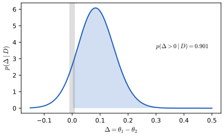
\[ p(\Delta\given D)=\int_0^1\mathrm{Beta}(\theta_1\given y_1+1,N_1-y_1+1)\,\mathrm{Beta}(\theta_1-\Delta\given y_2+1,N_2-y_2+1)\d\theta_1,\qquad p(\Delta\gt\epsilon\given D)=\int_\epsilon^\infty p(\Delta\given D)\d\Delta.\tag{5.63} \]Filling the gap 5.16: the posterior of the difference, and the left-handedness example pp. 188–189, Table 5.7
Derivation
Independent \(\theta_1,\theta_2\) with densities \(f_1,f_2\): the density of \(\Delta=\theta_1-\theta_2\) is the convolution \(f_\Delta(\Delta)=\int f_1(t)f_2(t-\Delta)\d t\) over \(t\in[\max(0,\Delta),\min(1,1+\Delta)]\) (the book writes this with an indicator and then drops it). Integrating the density over \(\Delta\gt\epsilon\) and exchanging the order of integration gives the one-dimensional form \(p(\Delta\gt\epsilon\given D)=\int_\epsilon^1f_1(t)F_2(t-\epsilon)\d t\), where \(F_2\) is the Beta cdf of \(\theta_2\); this is the form the code uses. The data of Table 5.7 are 9 left-handed of 52 men and 4 of 48 women, so the posteriors are \(\mathrm{Beta}(10,44)\) and \(\mathrm{Beta}(5,45)\), and the code obtains \(p(\theta_1\gt\theta_2\given D)=0.901\), matching the book, confirmed by a Monte Carlo estimate with \(2\times10^6\) draws.
5.3 Frequentist decision theory
p. 189 In the frequentist approach the unknown state of nature \(\theta\) is a fixed number and the data are random. Instead of conditioning on the observed \(x\), we ask how a decision procedure (an estimator \(\delta:\mathcal X\to\mathcal A\)) performs on average over data sets that \(\theta\) could have produced.
See also (companion course): All of Statistics 12.2, comparing risk functions, 12.4 minimax rules, 12.6 admissibility, 12.7 Stein’s paradox; Bayes rule and loss demo.
5.3.1 Computing the risk of an estimator
Definition 5.2 (frequentist risk, Bayes risk, maximum risk) (5.64), (5.74), (5.76)
The risk of an estimator \(\delta\) at \(\theta\) is the expected loss over data sets drawn from \(p(x\given\theta)\),
\[ R(\theta,\delta)\triangleq\E_{p(x|\theta)}[\ell(\theta,\delta(x))].\tag{5.64} \]Given a prior \(\pi_0\), the Bayes (integrated) risk is \(R_{\pi_0}(\delta)=\E_{\pi_0(\theta)}[R(\theta,\delta)]\) \((5.74)\), and the maximum risk is \(R_{\max}(\delta)=\sup_\theta R(\theta,\delta)\) \((5.76)\). A Bayes estimator minimises \(R_{\pi_0}\), a minimax estimator \(\delta_{\rm MM}\) minimises \(R_{\max}\).
5.3.1.1 Example
Estimate the mean of \(\N(\theta^*,\sigma^2=1)\) from \(N\) samples under squared error, so the risk is the mean squared error, which decomposes as \(\mse(\hat\theta\given\theta^*)=\var[\hat\theta]+\bias^2(\hat\theta)\) \((5.66)\). Five estimators are compared: \(\delta_1\) the sample mean; \(\delta_2\) the sample median; \(\delta_3=\theta_0\) a constant; and \(\delta_\kappa\), the posterior mean under the prior \(\N(\theta\given\theta_0,\sigma^2/\kappa)\) with \(\theta_0=0\),
\[ \delta_\kappa(x)=\frac N{N+\kappa}\bar x+\frac\kappa{N+\kappa}\theta_0=w\bar x+(1-w)\theta_0,\tag{5.65} \]for a weak prior (\(\kappa=1\)) and a stronger one (\(\kappa=5\)).
Filling the gap 5.17: the five risk functions, and the true variance of the median pp. 190–191, (5.67)–(5.73)
Derivation
Sample mean (5.67). \(\bar x\) is unbiased with variance \(\sigma^2/N\), so \(R=\sigma^2/N\), constant in \(\theta^*\).
Constant (5.69). No variance; bias \(\theta^*-\theta_0\): \(R=(\theta^*-\theta_0)^2\).
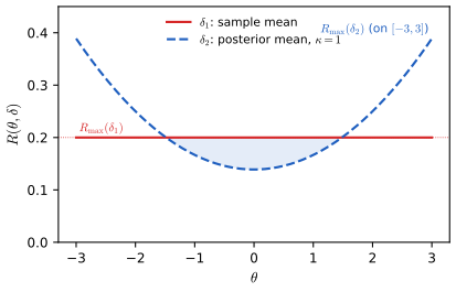
Posterior mean (5.70)–(5.73). With \(w=N/(N+\kappa)\), \[w\bar x+(1-w)\theta_0-\theta^*=w(\bar x-\theta^*)+(1-w)(\theta_0-\theta^*)\]. Squaring, the cross term has mean zero because \(\E(\bar x-\theta^*)=0\), so \[R=w^2\frac{\sigma^2}N+(1-w)^2(\theta_0-\theta^*)^2=\frac{N\sigma^2+\kappa^2(\theta_0-\theta^*)^2}{(N+\kappa)^2}\tag{5.73}\] (use \(w^2/N=N/(N+\kappa)^2\) and \(1-w=\kappa/(N+\kappa)\)). It beats the sample mean exactly when \((\theta^*-\theta_0)^2\lt\sigma^2(2N+\kappa)/(N\kappa)\): for \(N=5\), \(\kappa=1\) that is \(|\theta^*|\lt1.48\), the crossing seen in Figures 5.8 and 5.9. Its risk is smallest, \(N\sigma^2/(N+\kappa)^2\lt\sigma^2/N\), at \(\theta^*=\theta_0\) and grows without bound.
Sample median (5.68). The median of \(N\) draws from a symmetric density is unbiased (by symmetry of the sampling distribution about \(\theta^*\)), so its risk is its variance. The book uses the asymptotic value \(\pi/(2N)\) (for \(\sigma=1\)); here is why. Let \(f\) be the density and \(F_N(t)=\#\{x_i\le t\}\sim\mathrm{Bin}(N,F(t))\). The median is at most \(\theta^*+u/\sqrt N\) iff \(F_N(\theta^*+u/\sqrt N)\ge N/2\). With \(F(\theta^*+u/\sqrt N)\approx\frac12+f(\theta^*)u/\sqrt N\), the count has mean \(\approx N/2+f(\theta^*)u\sqrt N\) and standard deviation \(\approx\sqrt N/2\), so by the central limit theorem the probability tends to \(\Phi(2f(\theta^*)u)\): \(\sqrt N(\mathrm{med}-\theta^*)\to\N(0,1/(4f(\theta^*)^2))\). For the normal density \(f(\theta^*)=1/\sqrt{2\pi}\) and the limit variance is \(\pi/2\). It is only asymptotic. The exact variance of the median of \(N\) standard normals, by integrating against the order-statistic density, is \(0.2868\) for \(N=5\) (the asymptotic \(\pi/10=0.3142\) is 10% too large) and \(0.0734\) for \(N=20\) (\(\pi/40=0.0785\)). Figure 5.8 here uses the exact values; the code confirms them by simulation, by two-dimensional quadrature for even \(N\), and the limit \(N\,\mathrm{Var}\to\pi/2\) at \(N=1001\).
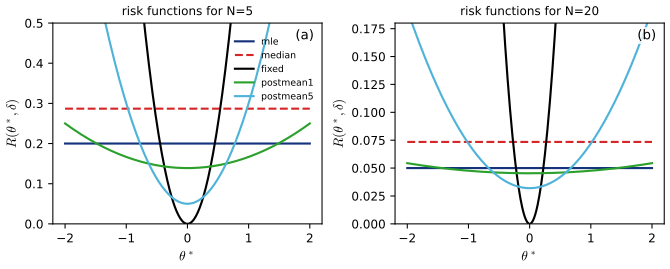
We see that the best estimator depends on the unknown \(\theta^*\): near \(\theta_0\) the constant or a posterior mean wins, in a middle range the posterior mean, far away the sample mean. The frequentist risk alone does not select an estimator, so two summaries are used.
5.3.1.2 Bayes risk
Average the risk over a prior: \[R_{\pi_0}(\delta)=\E_{\pi_0}[R(\theta,\delta)]=\iint\pi_0(\theta)p(x\given\theta)\ell(\theta,\delta(x))\d\theta\d x\] \((5.74)\). By Result 5.1 the minimiser is the pointwise Bayes rule \((5.75)\), so Bayesian decision theory and frequentist average risk agree.
5.3.1.3 Maximum risk
Avoiding the prior, take the worst case: \(R_{\max}(\delta)=\sup_\theta R(\theta,\delta)\) \((5.76)\), minimised by a minimax estimator. In Figure 5.9, \(\delta_1\) has the lower worst-case risk and is the minimax estimator even though \(\delta_2\) is better for most \(\theta\): minimax estimators are conservative, because they guard against an adversarial nature, which is rarely the situation in statistics (as opposed to game theory).
Result 5.8 (Bayes risk of the posterior mean; Bayes plus constant risk implies minimax; minimaxity of the sample mean) pp. 191–192
(a) Under the prior \(\theta\sim\N(\theta_0,\sigma^2/\kappa)\) the estimator \(\delta_\kappa\) has Bayes risk \(\sigma^2/(N+\kappa)\), smaller than the sample mean’s \(\sigma^2/N\). (b) If a Bayes estimator \(\delta_\pi\) has constant risk, \(R(\theta,\delta_\pi)=r\) for all \(\theta\), then it is minimax. (c) The sample mean of \(\N(\theta,\sigma^2)\) data is minimax for squared error. (d) More precisely than the book’s remark that “all minimax estimators are Bayes under a least favorable prior”: if the Bayes risks \(r_{\pi_k}\) of a sequence of priors tend to \(\sup_\theta R(\theta,\delta)\), then \(\delta\) is minimax; a minimax estimator need not itself be a Bayes rule for any proper prior (the sample mean is the example).
Proof
(a) Average (5.73) over \(\theta\): \(\E(\theta_0-\theta)^2=\sigma^2/\kappa\), so \(R_{\pi_0}=\frac{N\sigma^2+\kappa^2\sigma^2/\kappa}{(N+\kappa)^2}=\frac{\sigma^2(N+\kappa)}{(N+\kappa)^2}\). (The sample mean has constant risk \(\sigma^2/N\) and so Bayes risk \(\sigma^2/N\); \(\sigma^2/(N+\kappa)\lt\sigma^2/N\).) (b) For any \(\delta'\): \[\sup_\theta R(\theta,\delta')\ge\int R(\theta,\delta')\pi(\theta)\d\theta\ge\int R(\theta,\delta_\pi)\pi(\theta)\d\theta=r=\sup_\theta R(\theta,\delta_\pi)\], the middle inequality because \(\delta_\pi\) minimises the Bayes risk. (c,d) Take the prior \(\N(0,\tau^2)\). The posterior mean has posterior variance \(\sigma^2\tau^2/(\sigma^2+N\tau^2)\), which is its Bayes risk by Result 5.1. For any \(\delta'\), \[\sup_\theta R(\theta,\delta')\ge r_\tau=\sigma^2\tau^2/(\sigma^2+N\tau^2)\to\sigma^2/N\] as \(\tau\to\infty\). Hence \(\sup R(\delta')\ge\sigma^2/N=\sup R(\bar x)\), so \(\bar x\) is minimax. It is not Bayes for any proper prior (its Bayes risk \(\sigma^2/N\) equals the limit but is never attained at finite \(\tau\)). ∎
5.3.2 Consistent estimators
p. 192 Let \(x_1,\dots,x_N\) be iid from \(p(\cdot\given\theta^*)\) with identifiable parameters. An estimator \(\delta\) is consistent if \(\hat\theta(x_{1:N})\to\theta^*\) in probability as \(N\to\infty\). Consistency is a statement about the limit \(N\to\infty\); it says nothing about any fixed \(N\).
Filling the gap 5.18: unbiased but not consistent; consistency of the MLE; what happens under misspecification p. 192
Derivation
Unbiased and inconsistent. \(\delta(x_{1:N})=x_N\) has \(\E\delta=\mu\) but its distribution is that of one observation for every \(N\): it never concentrates, so it is not consistent. Conversely \(\bar x+1/N\) is biased but consistent.
The MLE is consistent (Wald, 1949) under: \(\Theta\) compact, \(\theta\mapsto\log p(x\given\theta)\) continuous with an integrable envelope \(\sup_\theta|\log p(x\given\theta)|\), and identifiability. Let \(\bar\ell_N(\theta)=\frac1N\sum_i\log p(x_i\given\theta)\) and \(\ell(\theta)=\E\log p(x\given\theta)\). By the uniform law of large numbers (continuity plus the envelope), \(\sup_\theta|\bar\ell_N-\ell|\to0\) almost surely. By the Gibbs inequality (Result 5.6), \(\ell(\theta^*)-\ell(\theta)=D_{\rm KL}(p_{\theta^*}\|p_\theta)\ge0\), with equality only at \(\theta=\theta^*\) by identifiability. Fix \(\epsilon\gt0\); on the compact set \(\{|\theta-\theta^*|\ge\epsilon\}\) the continuous function \(\ell\) is bounded away from \(\ell(\theta^*)\) by some \(\eta\gt0\). Once \(\sup|\bar\ell_N-\ell|\lt\eta/2\), the maximiser \(\hat\theta_N\) of \(\bar\ell_N\) cannot lie in that set, since \(\bar\ell_N(\hat\theta_N)\ge\bar\ell_N(\theta^*)\gt\ell(\theta^*)-\eta/2\gt\bar\ell_N(\theta)\) there. So \(\hat\theta_N\to\theta^*\).
Misspecification. If no \(\theta^*\) generates the data, say they come from \(p^\dagger\), the same argument shows \(\hat\theta_N\to\argmin_\theta D_{\rm KL}(p^\dagger\|p_\theta)\), since \(\E\log p_\theta\) differs from \(-D_{\rm KL}(p^\dagger\|p_\theta)\) by the constant \(-H(p^\dagger)\). This is the book’s remark that the MLE minimises the KL divergence between the empirical and the model distribution: it recovers the best member of the family in the KL sense, which is what one can hope for in practice. See also All of Statistics, Chapter 9.
5.3.3 Admissible estimators
\(\delta_1\) dominates \(\delta_2\) if \(R(\theta,\delta_1)\le R(\theta,\delta_2)\) for all \(\theta\), strictly for some \(\theta^*\). An estimator is admissible if no estimator dominates it. Wald (1947) proved, under technical conditions, that every admissible rule is a (generalised) Bayes rule or a limit of them (the complete class theorem), which is the deep reason why Bayesian procedures are the natural candidates.
In Figure 5.8 the sample median is always above the sample mean, so it is inadmissible. (For \(\N(\theta,1)\) data the mean attains the Cramér-Rao bound \(1/N\) among unbiased estimators, and the median is unbiased.) More surprising:
Filling the gap 5.19: a useless estimator can be admissible pp. 192–193
Let \(X\sim\N(\theta,1)\) and \(\delta_1(x)=\theta_0\), a constant. The book shows that \(\delta_1\) is admissible. The argument, with the assumption it needs made explicit:
Derivation
Suppose \(\delta_2\) satisfies \(R(\theta,\delta_2)\le R(\theta,\delta_1)=(\theta-\theta_0)^2\) for all \(\theta\). At \(\theta=\theta_0\) the right side is 0, so \[R(\theta_0,\delta_2)=\int(\delta_2(x)-\theta_0)^2p(x\given\theta_0)\d x=0\], and since \(p(x\given\theta_0)\gt0\) for every \(x\) (here a positive Gaussian density) this forces \(\delta_2(x)=\theta_0\) for almost every \(x\). So \(\delta_2=\delta_1\) almost everywhere and has the same risk everywhere: it cannot strictly dominate. The positivity of the density is essential (if the support depended on \(\theta\), the argument would need modification). Admissibility is therefore a weak requirement: it excludes obviously bad rules, but does not select good ones. Conversely, useful estimators can fail it, as next.
Result 5.9 (Stein’s paradox: the James-Stein estimator) p. 193, Stein (1956)
Let \(X\sim\N(\theta,\mathbf I_d)\) with \(d\ge3\) and squared error \(\ell(\theta,a)=\|\theta-a\|^2\). The sample (here the single observation) mean \(\delta_0(X)=X\) has risk \(d\) for all \(\theta\), but the James-Stein estimator \(\delta_{\rm JS}(X)=\big(1-\frac{d-2}{\|X\|^2}\big)X\) has risk \[ R(\theta,\delta_{\rm JS})=d-(d-2)^2\,\E\!\left[\frac1{\|X\|^2}\right]\lt d\quad\text{for every }\theta, \] so \(X\) is inadmissible. With \(K\sim\mathrm{Poisson}(\|\theta\|^2/2)\), \(\E[1/\|X\|^2]=\E[1/(d-2+2K)]\); at \(\theta=0\) the risk is \(2\). For \(d\le2\) the sample mean is admissible.
Proof
Write \(\delta_{\rm JS}=X+g(X)\), \(g(x)=-(d-2)x/\|x\|^2\). Then \[\|\delta_{\rm JS}-\theta\|^2=\|X-\theta\|^2+2(X-\theta)^\T g(X)+\|g(X)\|^2\]. The first term has mean \(d\); the last has mean \((d-2)^2\E\|X\|^{-2}\) (finite for \(d\ge3\)). For the cross term use Stein’s lemma: if \(Z\sim\N(\mu,1)\) and \(h\) is absolutely continuous with \(\E|h'(Z)|\lt\infty\), then \(\E[(Z-\mu)h(Z)]=\E[h'(Z)]\). (Proof: \((z-\mu)\varphi(z-\mu)=-\varphi'(z-\mu)\), so \[\int h(z)(z-\mu)\varphi(z-\mu)\d z=-[h\varphi]+\int h'\varphi\], and the boundary term vanishes.) Applying it to each coordinate (the singularity of \(g\) at 0 is integrable in dimension \(d\ge3\)) gives \(\E[(X-\theta)^\T g(X)]=\E[\nabla\cdot g(X)]\), and \[\nabla\cdot g(x)=-(d-2)\sum_i\Big(\frac1{\|x\|^2}-\frac{2x_i^2}{\|x\|^4}\Big)=-(d-2)\frac{d-2}{\|x\|^2}=-\frac{(d-2)^2}{\|x\|^2}.\] Therefore \[R=d-2(d-2)^2\E\|X\|^{-2}+(d-2)^2\E\|X\|^{-2}=d-(d-2)^2\E\|X\|^{-2}\], strictly below \(d\) because \(\|X\|^{-2}\gt0\). For the Poisson form, \(\|X\|^2\) is non-central \(\chi^2_d(\|\theta\|^2)\), which is a Poisson(\(\|\theta\|^2/2\)) mixture of central \(\chi^2_{d+2K}\) laws, and \(\E[1/\chi^2_\nu]=1/(\nu-2)\) for \(\nu\gt2\). At \(\theta=0\), \(\E\|X\|^{-2}=1/(d-2)\), giving risk \(d-(d-2)=2\). ∎
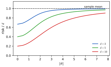
The paradox is that the components \(\theta_i\) may be unrelated (a mean height, a price, a rainfall), yet estimating them jointly beats estimating each separately by the sample mean. The resolution is that the total squared error is the criterion, and shrinking towards a common point trades a little bias for a larger variance reduction; this is the same mechanism as a prior in a hierarchical model, where the common point is learned from the data. See All of Statistics 12.7 for the empirical Bayes reading.
5.4 Empirical risk minimization
p. 193 In supervised learning the “state of nature” is the unknown joint distribution \(p^*(x,y)\) and the estimator is a prediction function \(f\), so the risk of \(f\) is the population risk
\[ R(f,p^*)=R(f)\triangleq\E_{p^*(x)p^*(y|x)}[\ell(y,f(x))].\tag{5.78} \]It cannot be computed; replacing \(p^*\) by the empirical distribution \(p_D=\frac1N\sum_n\delta_{(x_n,y_n)}\) \((5.79)\) gives the empirical risk \(R(f,D)=\frac1N\sum_n\ell(y_n,f(x_n))\) \((5.80)\), a random variable (it depends on the training set), and empirical risk minimisation (ERM)
\[ \hat f_{\rm ERM}=\argmin_{f\in\mathcal H}R(f,D)=\argmin_{f\in\mathcal H}\frac1N\sum_{n=1}^N\ell(y_n,f(x_n)).\tag{5.81} \]See also (companion course): Section 3.2, the bias-variance decomposition; All of Statistics, Chapter 4 for Hoeffding.
5.4.1.1 Approximation error versus estimation error
Let \(f^{**}=\argmin_fR(f)\) over all functions, \(f^*_{\mathcal H}=\argmin_{f\in\mathcal H}R(f)\) the best function in the class, and \(f^*_D=\argmin_{f\in\mathcal H}R(f,D)\) (a random function). Then
\[ \E_D[R(f^*_D)-R(f^{**})]=\underbrace{R(f^*_{\mathcal H})-R(f^{**})}_{\mathcal E_{\rm app}(\mathcal H)}+\underbrace{\E_D[R(f^*_D)-R(f^*_{\mathcal H})]}_{\mathcal E_{\rm est}(\mathcal H,N)}.\tag{5.83} \]Filling the gap 5.20: proof of (5.83), and a bound on the estimation error p. 194
Derivation
(5.83) is an add-and-subtract: \[R(f^*_D)-R(f^{**})=\{R(f^*_{\mathcal H})-R(f^{**})\}+\{R(f^*_D)-R(f^*_{\mathcal H})\}\], the first term not random; take \(\E_D\). The approximation error is a property of the class (richer \(\mathcal H\) gives smaller \(\mathcal E_{\rm app}\)); the estimation error is the price of finite data, decreasing in \(N\) and increasing with the size of \(\mathcal H\). A bound. Write \(\Delta=\sup_{f\in\mathcal H}|R(f,D)-R(f)|\). Then \[R(f^*_D)-R(f^*_{\mathcal H})=\{R(f^*_D)-R(f^*_D,D)\}+\{R(f^*_D,D)-R(f^*_{\mathcal H},D)\}+\{R(f^*_{\mathcal H},D)-R(f^*_{\mathcal H})\}\le\Delta+0+\Delta,\] because the middle term is \(\le0\) by the definition of \(f^*_D\) as the empirical minimiser. Hence \(\mathcal E_{\rm est}\le2\E\Delta\): uniform deviation of the empirical risk controls the estimation error (the reason for Section 5.4.4). The book also notes a third error from imperfect optimisation (Bottou and Bousquet, 2008).
5.4.1.2 Regularized risk
To limit overfitting add a penalty: \(R_\lambda(f,D)=R(f,D)+\lambda C(f)\) \((5.85)\), or for a parametric model \(R_\lambda(\theta,D)=R(\theta,D)+\lambda C(\theta)\) \((5.86)\), with \(\lambda\ge0\) a hyperparameter. With log loss and a negative-log-prior penalty,
\[R_\lambda(\theta,D)=-\frac1N\sum_{n=1}^N\log p(y_n\given x_n,\theta)-\lambda\log p(\theta),\tag{5.87}\]and minimising it is MAP estimation (for \(\lambda=1/N\), exactly: \[N R_{1/N}=-\sum\log p(y_n\given x_n,\theta)-\log p(\theta)=-\log p(\theta\given D)+\const\]; other \(\lambda\) correspond to the tempered prior \(p(\theta)^{N\lambda}\)).
5.4.2 Structural risk
To choose \(\lambda\) one might minimise \(\hat\lambda=\argmin_\lambda\min_\theta R_\lambda(\theta,D)\) \((5.88)\) (a bilevel problem). This fails: it always returns \(\lambda=0\) \((5.89)\). The cause is the optimism of the training error. If we knew the regularised population risk we could choose \(\lambda\) by structural risk minimisation (Vapnik, 1998); it is estimated either by cross-validation or by learning theory.
Filling the gap 5.21: why \(\hat\lambda=0\), and optimism of the training error p. 195
Derivation
\(\hat\lambda=0\). Let \(m(\lambda)=\min_\theta\{R(\theta,D)+\lambda C(\theta)\}\) with \(C\ge0\). For \(\lambda\le\lambda'\), \(R(\theta,D)+\lambda C(\theta)\le R(\theta,D)+\lambda'C(\theta)\) for every \(\theta\), so the minima are ordered: \(m\) is non-decreasing, and it is minimised at \(\lambda=0\). (The training objective can only get worse when a penalty is added.) Optimism. Let \(\hat f=f^*_D\) be the empirical risk minimiser over \(\mathcal H\). For any fixed \(f\in\mathcal H\), \(R(\hat f,D)\le R(f,D)\). Taking \(f=f^*_{\mathcal H}\) (not random) and expectations, \(\E R(\hat f,D)\le\E R(f^*_{\mathcal H},D)=R(f^*_{\mathcal H})\), and by definition of \(f^*_{\mathcal H}\) as the best member of \(\mathcal H\), \(R(f^*_{\mathcal H})\le R(\hat f)\) pointwise since \(\hat f\in\mathcal H\). Hence \[\E[R(\hat f,D)]\le R(f^*_{\mathcal H})\le\E[R(\hat f)]:\] the expected training risk underestimates the expected population risk; the gap is the optimism. Numerically (code): degree-4 least-squares polynomials on 12 noisy points, averaged over 2000 data sets, have mean training risk below mean test risk. For linear least squares with known variance the gap is exactly \(2k\sigma^2/N\) (the origin of AIC, Gap 5.13).
5.4.3 Cross-validation
Split the data into a training set \(D_{\rm train}\) and a validation set \(D_{\rm valid}\) and use the validation risk \(R^{\rm val}_\lambda\triangleq R_0(\hat\theta_\lambda(D_{\rm train}),D_{\rm valid})\) \((5.91)\), the unregularised empirical risk on held-out data, as the estimate of the population risk. With few data both the training and the estimate suffer, so one uses \(K\)-fold cross-validation
\[ R^{\rm cv}_\lambda\triangleq\frac1K\sum_{k=1}^KR_0(\hat\theta_\lambda(D_{-k}),D_k),\tag{5.92} \]where \(D_k\) is the \(k\)-th fold and \(D_{-k}\) the rest. \(K=N\) is leave-one-out. One chooses \(\hat\lambda=\argmin_\lambda R^{\rm cv}_\lambda\) and then refits on all the data.
Filling the gap 5.22: leave-one-out without refitting p. 196
The book notes that cross-validation is slow because the model is refitted \(K\) times. For ridge regression (and any linear smoother) leave-one-out needs no refits.
Derivation
Let \(\mathbf A=\mathbf X^\T\mathbf X+\lambda\mathbf I\), \(\hat{\mathbf w}=\mathbf A^{-1}\mathbf X^\T\mathbf y\), \(e_i=y_i-\mathbf x_i^\T\hat{\mathbf w}\) and \(h_{ii}=\mathbf x_i^\T\mathbf A^{-1}\mathbf x_i\) (the diagonal of the hat matrix \(\mathbf H=\mathbf X\mathbf A^{-1}\mathbf X^\T\)). Removing observation \(i\) replaces \(\mathbf A\) by \(\mathbf A-\mathbf x_i\mathbf x_i^\T\) and \(\mathbf X^\T\mathbf y\) by \(\mathbf X^\T\mathbf y-\mathbf x_iy_i\). By the Sherman-Morrison formula \((\mathbf A-\mathbf x_i\mathbf x_i^\T)^{-1}=\mathbf A^{-1}+\frac{\mathbf A^{-1}\mathbf x_i\mathbf x_i^\T\mathbf A^{-1}}{1-h_{ii}}\), so
\[\hat{\mathbf w}_{-i}=\hat{\mathbf w}-\mathbf A^{-1}\mathbf x_iy_i+\frac{\mathbf A^{-1}\mathbf x_i(\mathbf x_i^\T\hat{\mathbf w}-h_{ii}y_i)}{1-h_{ii}}=\hat{\mathbf w}-\frac{\mathbf A^{-1}\mathbf x_i\,e_i}{1-h_{ii}},\]
and the held-out residual is \(y_i-\mathbf x_i^\T\hat{\mathbf w}_{-i}=e_i+\frac{h_{ii}e_i}{1-h_{ii}}=\frac{e_i}{1-h_{ii}}\). So the leave-one-out squared error (PRESS) is \(\frac1N\sum_i\{e_i/(1-h_{ii})\}^2\), computed from a single fit. The code checks the identity against \(N\) explicit refits (loo_press_residuals) to \(10^{-10}\). Generalised cross-validation replaces \(h_{ii}\) by their average \(\Tr\mathbf H/N\).
5.4.4 Statistical learning theory *
Cross-validation is slow; statistical learning theory (SLT) instead gives analytic upper bounds on the generalisation error that hold with high probability. If \(R(\hat h)\le\epsilon\) with probability at least \(1-\delta\), the hypothesis is probably approximately correct (PAC) and the class is PAC learnable.
5.4.4.1 Bounding the generalization error
Result 5.10 (Theorem 5.4.1: uniform deviation for a finite class; Hoeffding’s inequality) pp. 196–197, (5.93)–(5.97)
Let \(\mathcal H\) be a finite class of binary classifiers and \(D\) an iid sample of size \(N\) from any \(p^*\); \(R(h,D)=\frac1N\sum_i\mathbb I(h(x_i)\ne y_i)\), \(R(h)=\E\,\mathbb I(h(x)\ne y)\). Then for every \(\epsilon\gt0\)
\[ \Pr\Big(\max_{h\in\mathcal H}|R(h)-R(h,D)|\gt\epsilon\Big)\le2|\mathcal H|e^{-2N\epsilon^2}.\tag{5.93} \]Consequently, with probability at least \(1-\delta\), every \(h\in\mathcal H\) has \(|R(h)-R(h,D)|\le\sqrt{\ln(2|\mathcal H|/\delta)/(2N)}\), the ERM \(\hat h\) satisfies \(R(\hat h)\le R(h^*_{\mathcal H})+2\sqrt{\ln(2|\mathcal H|/\delta)/(2N)}\), and \(N\ge\ln(2|\mathcal H|/\delta)/(2\epsilon^2)\) samples guarantee uniform deviation at most \(\epsilon\).
Proof (including Hoeffding’s inequality, which the book quotes)
Hoeffding’s lemma. If \(\E X=0\) and \(a\le X\le b\) then \(\E e^{sX}\le e^{s^2(b-a)^2/8}\) for all \(s\in\R\). By convexity of \(x\mapsto e^{sx}\), \(e^{sx}\le\frac{b-x}{b-a}e^{sa}+\frac{x-a}{b-a}e^{sb}\) on \([a,b]\); taking expectations with \(\E X=0\), \(\E e^{sX}\le\frac{b}{b-a}e^{sa}-\frac a{b-a}e^{sb}=e^{\phi(u)}\) where \(u=s(b-a)\), \(p=-a/(b-a)\) and \(\phi(u)=-pu+\ln(1-p+pe^u)\). Now \(\phi(0)=0\), \(\phi'(0)=0\), \(\phi''(u)=q(1-q)\le\frac14\) with \(q=pe^u/(1-p+pe^u)\), so by Taylor with remainder \(\phi(u)\le u^2/8\), i.e. the lemma.
Hoeffding’s inequality (5.94). Let \(E_1,\dots,E_N\) be independent in \([0,1]\) with mean \(\theta\) and \(\bar E=\frac1N\sum E_i\). By Markov’s inequality applied to \(e^{sN(\bar E-\theta)}\) for \(s\gt0\) and independence, \[\Pr(\bar E-\theta\ge\epsilon)\le e^{-sN\epsilon}\prod_i\E e^{s(E_i-\theta)}\le\exp(-sN\epsilon+Ns^2/8)\], using the lemma with \(b-a=1\). Minimising over \(s\) (take \(s=4\epsilon\)) gives \(e^{-2N\epsilon^2}\). The lower tail is the same by symmetry, so \(\Pr(|\bar E-\theta|\ge\epsilon)\le2e^{-2N\epsilon^2}\).
The theorem. For a fixed \(h\) the indicators \(\mathbb I(h(x_i)\ne y_i)\) are iid \(\mathrm{Ber}(R(h))\) with mean \(R(h)\) and average \(R(h,D)\): so \(\Pr(|R(h)-R(h,D)|\gt\epsilon)\le2e^{-2N\epsilon^2}\) \((5.96)\). The event \(\{\max_h|\cdot|\gt\epsilon\}\) is the union over \(h\in\mathcal H\) of the events \(\{|R(h)-R(h,D)|\gt\epsilon\}\), and the union bound \(\Pr(\bigcup_iA_i)\le\sum_i\Pr(A_i)\) gives (5.93) \((5.95)\)–\((5.97)\). Setting the right side equal to \(\delta\) and solving for \(\epsilon\) gives the second statement; for the third, on the event of the second statement \[R(\hat h)\le R(\hat h,D)+\epsilon_\delta\le R(h^*_{\mathcal H},D)+\epsilon_\delta\le R(h^*_{\mathcal H})+2\epsilon_\delta\] (the middle step is the definition of ERM); the sample size is the same equation solved for \(N\). ∎
The bound grows with \(\ln|\mathcal H|\) and falls with \(N\), confirming that the optimism of the training error increases with the richness of the class and decreases with the sample size. For \(|\mathcal H|=1000\), \(\epsilon=0.05\), \(\delta=0.01\) one needs \(N\ge\ln(2\times10^5)/(2\cdot0.0025)\approx2441.2\), so 2442.
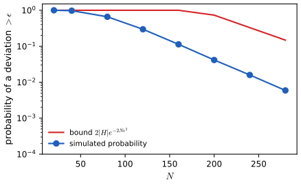
5.4.4.2 VC dimension
For an infinite class one cannot use \(|\mathcal H|\). The VC dimension \(d_{\rm VC}\) (Vapnik and Chervonenkis) is the size of the largest set of points that \(\mathcal H\) can label in all \(2^{d}\) ways (shatter); for example, the half-planes in \(\R^2\) have \(d_{\rm VC}=3\). It replaces \(\ln|\mathcal H|\) by \(d_{\rm VC}\ln N\) in bounds of the form \[R(h)\le R(h,D)+O(\sqrt{(d_{\rm VC}\ln N+\ln(1/\delta))/N})\] (Vapnik, 1998). The book notes that the bounds are usually loose and VC dimensions hard to compute for modern models, so they are of limited practical value.
5.5 Frequentist hypothesis testing *
p. 198 A frequentist test decides whether a null model \(H_0\) describes the data, relative to an alternative \(H_1\); it is a binary decision rule and so inherits the language of Sections 5.1.2 and 5.1.3.
See also (companion course): All of Statistics 10.2, p-values, 10.5 the permutation test, 10.6 the likelihood ratio test, 10.10.1 the Neyman-Pearson lemma.
5.5.1 Likelihood ratio test
With a uniform prior over \(H_0,H_1\) and zero-one loss, the Bayes rule accepts \(H_0\) iff \(p(D\given H_0)/p(D\given H_1)\gt1\): the likelihood ratio test. Example: comparing Gaussian means. Data \(x_1,\dots,x_N\) come from \(\N(\mu_0,\sigma^2)\) or \(\N(\mu_1,\sigma^2)\), with known shared variance. For compound hypotheses, where parameters are not fully specified, the Bayesian integrates them out, which is expensive and prior sensitive; the maximum likelihood ratio test maximises them instead \((5.100)\).
Filling the gap 5.23: the Gaussian likelihood ratio, the threshold, and the error rates pp. 198–199, (5.98)–(5.104)
Derivation
Using \[\sum_n(x_n-\mu)^2=\sum_n(x_n-\bar x)^2+N(\bar x-\mu)^2\], \[\frac{p(D\given H_0)}{p(D\given H_1)}=\exp\Big\{-\frac1{2\sigma^2}\Big(\sum_n(x_n-\mu_0)^2-\sum_n(x_n-\mu_1)^2\Big)\Big\}=\exp\Big\{\frac1{2\sigma^2}\big(2N\bar x(\mu_0-\mu_1)+N\mu_1^2-N\mu_0^2\big)\Big\}.\tag{5.98, 5.99}\] The data enter only through \(\bar x\), a sufficient statistic. If \(\mu_0\lt\mu_1\), the exponent is decreasing in \(\bar x\), so the ratio exceeds 1 iff \(\bar x\lt x^*=(\mu_0+\mu_1)/2\) (the point where the two densities of \(\bar x\) cross) for equal priors; a general threshold on the ratio is a threshold on \(\bar x\). Error rates. Fix the threshold at \(x^*\) (any value). Under \(H_0\), \(\bar x\sim\N(\mu_0,\sigma^2/N)\), so the type I error (false positive) is \(\alpha=\Pr(\bar x\gt x^*\given H_0)=1-\Phi\big(\frac{x^*-\mu_0}{\sigma/\sqrt N}\big)\) \((5.101)\)–\((5.103)\); demanding a size \(\alpha\) forces \(x^*=\mu_0+z_\alpha\sigma/\sqrt N\) with \(z_\alpha=\Phi^{-1}(1-\alpha)\). The type II error is \(\beta=\Pr(\bar x\lt x^*\given H_1)=\Phi\big(\frac{x^*-\mu_1}{\sigma/\sqrt N}\big)\) \((5.104)\), so the power is \(1-\beta=\Phi\big(\frac{(\mu_1-\mu_0)\sqrt N}\sigma-z_\alpha\big)\). It increases with the effect size \(|\mu_1-\mu_0|/\sigma\), with \(N\), and with \(\alpha\); at \(\mu_1=\mu_0\) the power is \(\alpha\). Equal-prior zero-one loss balances the two errors (\(\alpha=\beta\) at \(x^*=(\mu_0+\mu_1)/2\)); fixing \(\alpha\) at 0.05 instead is a convention, not a consequence of decision theory. The maximum LRT. In (5.100) the ratio of maximised likelihoods \(\Lambda=\max_{H_0}p_\theta(D)/\max_{H_1}p_\theta(D)\) has, under \(H_0\) and regularity conditions, \(-2\log\Lambda\to\chi^2_{r}\) (Wilks’ theorem, \(r\) the difference in dimension), which fixes the threshold without a prior; see All of Statistics 10.6.
5.5.2 Type I vs type II errors and the Neyman-Pearson lemma
A type I error (false positive) rejects a true null, with probability \(\alpha\), the significance or size of the test; a type II error (false negative) accepts a false null, with probability \(\beta\); the power is \(1-\beta\), the true positive rate. If test B has at least the power of test A at every alternative and the same size, B dominates A (Figure 5.10b).
Result 5.11 (Neyman-Pearson lemma) p. 200
Let \(H_0\) and \(H_1\) be simple with densities \(p_0,p_1\). Among all tests \(\phi:\mathcal X\to\{0,1\}\) (1 = reject) with size \(\E_0\phi\le\alpha\), the test \(\phi^*=\mathbb I\{p_1(x)/p_0(x)\gt k\}\) with \(k\) chosen so that \(\E_0\phi^*=\alpha\) has the largest power \(\E_1\phi\): the likelihood ratio test is most powerful.
Proof
For every \(x\), \((\phi^*(x)-\phi(x))(p_1(x)-kp_0(x))\ge0\): if \(p_1\gt kp_0\) then \(\phi^*=1\ge\phi\); if \(p_1\lt kp_0\) then \(\phi^*=0\le\phi\); if equal the product is 0. Integrate over \(x\): \[\E_1\phi^*-\E_1\phi\ge k(\E_0\phi^*-\E_0\phi)=k(\alpha-\E_0\phi)\ge0\] since \(\phi\) has size at most \(\alpha\) (and \(k\ge0\)). (For discrete \(x\) the size \(\alpha\) may require randomising on the boundary \(p_1=kp_0\); the same proof applies with \(\phi\in[0,1]\).) ∎
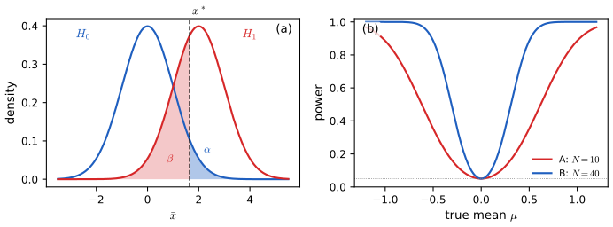
5.5.3 Null hypothesis significance testing (NHST) and p-values
When no alternative is available, define a test statistic \(\mathrm{test}(D)\) and compare it with its distribution under \(H_0\). The p-value is
\[ \mathrm{pval}\triangleq\Pr(\mathrm{test}(\tilde D)\ge\mathrm{test}(D)\given\tilde D\sim H_0).\tag{5.105} \]One rejects at the significance level \(\alpha\) (traditionally 0.05) if \(\mathrm{pval}\lt\alpha\). For the Wald statistic \(z=(\hat\theta-\theta_0)/\widehat{\rm se}\) the two-sided p-value is \(\approx2\Phi(-|z|)\). When the null distribution is not available analytically one uses the bootstrap, or, for two samples, the permutation test: randomly permute the pooled data labels, recompute \(|\bar X-\bar Y|\) and take the tail fraction.
Filling the gap 5.24: why rejecting at \(p\lt\alpha\) has type I error \(\alpha\), and why the permutation p-value is valid pp. 200–201
Derivation
Uniformity. Let \(T\) be a continuous test statistic with null cdf \(F_0\) (large values favour \(H_1\)), so \(\mathrm{pval}=1-F_0(T)\). Under \(H_0\), \(F_0(T)\sim U(0,1)\) (the probability integral transform), hence \(\Pr(\mathrm{pval}\le u)=\Pr(F_0(T)\ge1-u)=u\): the p-value is uniform on \([0,1]\) under \(H_0\), and the rule “reject iff pval \(\le\alpha\)” has type I error exactly \(\alpha\). The p-value is thus the smallest \(\alpha\) at which the observed data would lead to rejection. For discrete \(T\) the rule is conservative: \(\Pr(\mathrm{pval}\le\alpha)\le\alpha\). Wald. By asymptotic normality of the MLE (Section 4.7.2), \(z\) is approximately \(\N(0,1)\) under \(H_0\), so \(\Pr(|z_{\rm null}|\ge|z_{\rm obs}|)\approx2\Phi(-|z_{\rm obs}|)\); e.g. \(z=1.96\) gives \(0.04999\).
Permutation test. Under \(H_0:P_X=P_Y\) the pooled sample of \(m+n\) values is exchangeable, so the observed labelling is one of \(\binom{m+n}m\) equally likely ones. If \(T_{\rm obs}\) is the statistic of the original labelling and \(T_1,\dots,T_B\) those of \(B\) random permutations, then \(T_{\rm obs},T_1,\dots,T_B\) are exchangeable, so the rank of \(T_{\rm obs}\) among them is uniform on \(\{1,\dots,B+1\}\), and \(p=\frac{1+\#\{b:T_b\ge T_{\rm obs}\}}{B+1}\) satisfies \(\Pr(p\le u)\le u\): it is an exact finite-sample p-value, with no distributional assumption (including no normality). The “+1” in numerator and denominator counts the observed labelling itself and is what makes it exact. The code compares such a p-value with Welch’s t-test on simulated data and finds them close.
5.5.4 p-values considered harmful
A small p-value is often read as: “If \(H_0\) were true this statistic would be unlikely; it occurred; so \(H_0\) is probably false.” This is invalid. Cohen’s parallel: “If a person is American, he is probably not a member of Congress; this person is a member of Congress; so he is probably not American” is absurd, while the argument with “Martian” and “is not” is valid (modus tollens). The difference: a p-value measures \(\Pr(\text{data}\given H_0)\), and to get \(p(H_0\given D)\) we need Bayes’ rule,
\[ p(H_0\given D)=\frac{p(D\given H_0)p(H_0)}{p(D\given H_0)p(H_0)+p(D\given H_1)p(H_1)}=\frac{\mathrm{LR}}{\mathrm{LR}+1}\ \text{(equal priors)},\quad\mathrm{LR}=\frac{p(D\given H_0)}{p(D\given H_1)}.\tag{5.106, 5.107} \]In the Congress example \(p(D\given H_1)=0\) (only Americans serve), so \(\mathrm{LR}=\infty\) and \(p(H_0\given D)=1\). NHST ignores both \(p(D\given H_1)\) and the prior. The clinical-trial example (Table 5.8). Of 200 trials, 20 of the drugs work; the test has type I error \(\alpha=9/180=0.05\) and type II error \(\beta=4/20=0.2\). Then
\[ p(H_0\given\text{significant})=\frac{\alpha\,p(H_0)}{\alpha\,p(H_0)+(1-\beta)\,p(H_1)}.\tag{5.108–5.110} \]With a prior \(p(H_0)=0.9\) this is \(0.045/(0.045+0.08)=0.36\), seven times larger than the 5 per cent people associate with \(p\lt0.05\). Equivalently, of the 25 “significant” results in the table, 9 (36 per cent) are false discoveries.
Result 5.12 (a p-value of 0.05 leaves \(p(H_0\given D)\ge0.29\)) p. 201, Sellke, Bayarri and Berger (2001)
Let the p-value have density \(f(p\given\xi)=\xi p^{\xi-1}\), \(0\lt\xi\le1\) under the alternative (a monotone decreasing family on \([0,1]\), uniform for \(\xi=1\) which is the null). Then for \(p\lt1/e\) the Bayes factor in favour of \(H_0\) satisfies \(B_{0,1}\ge-e\,p\ln p\), and so, with equal prior probabilities, \[ p(H_0\given D)\ge\Big(1+\frac1{-e\,p\ln p}\Big)^{-1}. \] For \(p=0.05\) the bound is \(0.289\); for \(p=0.01\), \(0.111\); for \(p=0.001\), \(0.0184\).
Proof
The null density of the p-value is uniform: \(f(p\given H_0)=1\). So \(B_{0,1}=1/f(p\given\xi)=1/(\xi p^{\xi-1})\) for the alternative indexed by \(\xi\), and the smallest Bayes factor against \(H_0\) over \(\xi\) comes from maximising \(g(\xi)=\xi p^{\xi-1}\). Then \(g'(\xi)=p^{\xi-1}(1+\xi\ln p)\) vanishes at \(\xi^*=-1/\ln p\), which lies in \((0,1]\) exactly when \(p\le1/e\), and \[g(\xi^*)=\xi^*p^{-1}p^{\xi^*}=\xi^*p^{-1}e^{-1}=-1/(e\,p\ln p)\], because \(p^{-1/\ln p}=e^{-1}\). \(g\) is increasing before \(\xi^*\) and decreasing after, so this is the maximum. Hence \(B_{0,1}\ge1/g(\xi^*)=-e\,p\ln p\) for every alternative of the family (in particular for any mixture of them). With equal priors \(p(H_0\given D)=B_{0,1}/(1+B_{0,1})\), increasing in \(B_{0,1}\), which gives the bound. ∎
So the book’s statement that with \(p=0.05\) the posterior probability of \(H_0\) “can be as high as 30% or more, even with a uniform prior” is exactly right for this calibration: the lower bound is \(29\%\). It is a bound over a flexible class; for a specific alternative it can be higher still.
Filling the gap 5.25: the Lindley paradox and the dependence of p-values on the stopping rule pp. 201–202
Derivation
Lindley’s paradox. For the coin of Section 5.2.1.1 with \(N\) tosses and \(N_1=N/2+z\sqrt N/2\) heads, the z-score is fixed at \(z=1.96\) (so the two-sided p-value is about 0.05 for every \(N\)), but the Bayes factor changes with \(N\). From (5.47) with a uniform prior, \[B_{0,1}=(N+1)\mathrm{Bin}(N_1;N,\frac12)\approx(N+1)\sqrt{\frac2{\pi N}}e^{-z^2/2}\approx\sqrt{\frac{2N}\pi}\,e^{-z^2/2}\], which grows like \(\sqrt N\). For \(N=10\,000\), \(N_1=5100\) (\(z=2\), p = 0.0466): the code gives \(B_{0,1}=10.8\) and \(p(M_0\given D)=0.915\): the “significant” result favours the fair coin by a factor 10. The reason: under the sharp null the head fraction is within \(\pm1/\sqrt N\) of \(\frac12\); a free coin spreads its probability over \([0,1]\), so a deviation of \(0.01\) is about \(10\times\) less probable under \(M_1\) than under \(M_0\). A small effect that is significant with large \(N\) can still be evidence for the null against a diffuse alternative (Figure 5.S5, right).
Stopping rules. Observe a sequence with 9 heads and 3 tails. (i) If \(N=12\) was fixed in advance, the one-sided p-value for \(H_0:\theta=\frac12\) against \(\theta\gt\frac12\) is \(\Pr(\mathrm{Bin}(12,\frac12)\ge9)=0.073\), not significant. (ii) If the experimenter planned to stop at the third tail, the number of heads is negative binomial and the p-value is \[\Pr(\text{at least 9 heads before the 3rd tail})=0.033\], significant. The likelihood in both cases is \(\propto\theta^9(1-\theta)^3\), so the data are the same, only the sampling plan (hypothetical other data sets) differs. Bayes factors and posteriors depend on the data only through the likelihood, and so are the same in both cases: this is the likelihood principle of Section 5.5.5.
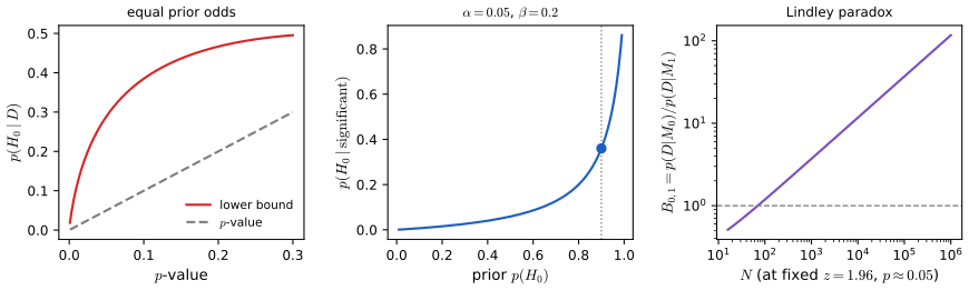
5.5.5 Why isn’t everyone a Bayesian?
The book collects the counter-intuitive behaviours of frequentist inference (p-values, confidence intervals, stopping rules) and traces them to the fact that frequentist inference violates the likelihood principle: inference should depend on the data only through the likelihood of the observed data, not on hypothetical data sets that were not observed. Bayesian inference satisfies it (Gap 5.25). Efron (1986) asked why everyone is not a Bayesian: historically, everyone was (Laplace, Gauss); frequentism dominated the 20th century, partly because of computation, which is a smaller barrier today. The remaining objection is that Bayes is only as good as the model; but so is frequentism, whose sampling distributions also rest on a model, and one can check models empirically (cross-validation, calibration, posterior predictive checks). The book closes with Rubin (1984): be Bayesian in principle and calibrated to the real world in practice.
Filling the gap 5.26: sampling distributions of the MLE equal posteriors under a non-informative prior p. 204, Box and Tiao (1973)
The book remarks that for common models the sampling distribution of the MLE is identical to the posterior under a non-informative prior, which is why frequentist and Bayesian intervals often agree numerically. The simplest case, with proof:
Derivation
Let \(x_1,\dots,x_N\sim\N(\theta,\sigma^2)\) with \(\sigma\) known and \(\hat\theta=\bar x\). Sampling distribution (for fixed \(\theta\)): \(\hat\theta\sim\N(\theta,\sigma^2/N)\), so \[\Pr(\bar x-1.96\sigma/\sqrt N\le\theta\le\bar x+1.96\sigma/\sqrt N)=0.95\] over repeated data. Posterior under the flat prior \(p(\theta)\propto1\): \(p(\theta\given D)\propto\exp\{-N(\bar x-\theta)^2/2\sigma^2\}\), i.e. \(\theta\given D\sim\N(\bar x,\sigma^2/N)\), so the credible interval \(\bar x\pm1.96\sigma/\sqrt N\) has posterior probability 0.95. The two intervals are the same set, with different probabilistic meanings. The reason is a pivot: \(\bar x-\theta\) has the same \(\N(0,\sigma^2/N)\) distribution whether \(\bar x\) is regarded as random with \(\theta\) fixed or \(\theta\) as random with \(\bar x\) fixed (the density depends on \(\bar x\) and \(\theta\) only through their difference, and the flat prior is invariant to translation). The same holds for every location family with a flat prior, and for scale families with the prior \(1/\sigma\). The coincidence breaks down when the likelihood principle is violated, as with stopping rules (Gap 5.25), or with a boundary or a prior that carries information.
Exercises
All four exercises of Chapter 5 (book pages 204–205), restated in my own words, with complete solutions (hidden). Daggers in the book mark harder problems. Each solution was worked out independently, and the computational ones are checked with the code.
Exercise 5.1 (reject option in classifiers). A classifier may choose among \(C\) class labels \(1,\dots,C\) or the reject action \(C+1\). With true class \(Y=j\), the loss is \(0\) if the label \(i=j\) is chosen, \(\lambda_r\) for rejecting and \(\lambda_s\) for any other label (a substitution error), as in (5.111). (a) Show that the minimum-risk rule picks class \(j\) when \(p(Y=j\given x)\ge p(Y=k\given x)\) for all \(k\) and \(p(Y=j\given x)\ge1-\lambda_r/\lambda_s\), and rejects otherwise. (b) Describe qualitatively what happens as \(\lambda_r/\lambda_s\) increases from 0 to 1.
Solution
(a) Choosing label \(i\le C\) has posterior risk \[\sum_{j\ne i}\lambda_sp(Y=j\given x)=\lambda_s\{1-p(Y=i\given x)\}\], smallest for the most probable class \(j^*\), with value \(\lambda_s(1-p^*)\), \(p^*=p(Y=j^*\given x)\). Rejecting has risk \(\lambda_r\) whatever the class. The best action is the one with the smaller risk: answer \(j^*\) iff \(\lambda_s(1-p^*)\le\lambda_r\), i.e. \(p^*\ge1-\lambda_r/\lambda_s\); otherwise reject. This is Chow’s rule, Result 5.3 (with ties broken in favour of answering). (b) The threshold \(1-\lambda_r/\lambda_s\) falls from 1 (at \(\lambda_r=0\): rejection is free, so reject unless certain) to 0 (at \(\lambda_r=\lambda_s\): rejection costs as much as a mistake, so never reject, since answering the most probable class is at least as good). The reject region (the set of \(x\) where \(p^*\lt\) threshold) shrinks monotonically, and for \(\lambda_r\ge\lambda_s\) it is empty. For two classes the reject region is the interval of \(x\) around the decision boundary where the posteriors are in \((\lambda_r/\lambda_s,1-\lambda_r/\lambda_s)\): in the binormal case of Figure 5.1, with \(\lambda_r/\lambda_s=0.2\), the interval has width \(\ln4=1.39\); the width goes to 0 as the ratio goes to \(1/2\) (for two classes \(p^*\ge1/2\) always, so for a ratio above \(1/2\) there is no rejection even though the threshold is above 0). The demonstration reports the loss: rejecting reduces the expected loss from 0.227 to 0.151 at \(\lambda_r=0.2\) (computed by the code and the page).
Exercise 5.2 (newsvendor problem). A seller buys \(Q\) items at cost \(C\) each and sells at price \(P\); demand \(D\) is random with density \(f\) and cdf \(F\). If \(D\gt Q\) all \(Q\) are sold, profit \((P-C)Q\); if \(D\lt Q\), \(D\) are sold and the \(C(Q-D)\) spent on the unsold items is wasted. The expected profit is \[ \E\pi(Q)=\int_Q^\infty(P-C)Qf(D)\d D+\int_0^Q(P-C)Df(D)\d D-\int_0^QC(Q-D)f(D)\d D.\tag{5.112} \] Simplify it and show that the optimal \(Q^*\) satisfies \(F(Q^*)=(P-C)/P\) \((5.113)\).
Solution
Let \(m(Q)=\int_0^QDf(D)\d D\). Then \(\int_Q^\infty f=1-F(Q)\) and \(\int_0^Q(Q-D)f=QF(Q)-m(Q)\), so \[\E\pi(Q)=(P-C)Q\{1-F(Q)\}+(P-C)m(Q)-C\{QF(Q)-m(Q)\}=(P-C)Q-PQF(Q)+Pm(Q)\] (the terms in \(CQF\) combine: \(-(P-C)QF-CQF=-PQF\); the terms in \(m\): \((P-C)m+Cm=Pm\)). Equivalently \(\E\pi=P\,\E\min(Q,D)-CQ\): revenue on units actually sold minus the purchase cost. Differentiate, with \(m'(Q)=Qf(Q)\): \[\frac{\d}{\d Q}\E\pi=(P-C)-PF(Q)-PQf(Q)+PQf(Q)=P-C-PF(Q)\]. Setting it to 0 gives \(F(Q^*)=(P-C)/P\). The second derivative is \(-Pf(Q)\le0\), so \(\E\pi\) is concave and the stationary point is the maximum. It is the quantile of the demand at the critical ratio \((P-C)/P\): the margin divided by the price, the probability of not running out of stock. Computation. With demand \(\N(100,20^2)\), \(P=10\), \(C=6\): \(F(Q^*)=0.4\), so \(Q^*=100+20\,\Phi^{-1}(0.4)=94.93\), expected profit \(322.73\) (against \(320.21\) for ordering the mean demand, 100). The code (
newsvendor_Q,newsvendor_expected_profit) maximises (5.112) numerically and obtains the same \(Q^*\) to \(10^{-4}\), and a Monte Carlo average of \(P\min(Q,D)-CQ\) over \(10^6\) demands matches the formula. In decision-theoretic terms: up to a term not depending on \(Q\), the negative profit is the loss \[ \ell(Q,D)=(P-C)(D-Q)_++C(Q-D)_+ \] (a cost \(P-C\) per unit short, \(C\) per unit left over), an asymmetric absolute loss whose Bayes action is the quantile of level \((P-C)/P\), just as the median is for \(\ell_1\) (Result 5.5, and the threshold of Result 5.2).Exercise 5.3 (Bayes factors and ROC curves). Let \(B=p(D\given H_1)/p(D\given H_0)\) be the Bayes factor for model 1. One ROC curve is made by thresholding \(B\), another by thresholding \(p(H_1\given D)\). Are they the same or different? Explain.
Solution
They are the same. With priors \(\pi_0,\pi_1\), \(p(H_1\given D)=\pi_1B/(\pi_1B+\pi_0)\), a strictly increasing function of \(B\) (its derivative in \(B\) is \(\pi_0\pi_1/(\pi_1B+\pi_0)^2\gt0\)). For every threshold \(t\) on \(B\), the rule \(B\ge t\) is the same as \(p(H_1\given D)\ge\pi_1t/(\pi_1t+\pi_0)\), so the two families of classifiers are identical sets of rules, and the FPR and TPR of each rule do not depend on how it was labelled. Hence the same set of \((\mathrm{FPR},\mathrm{TPR})\) points, the same curve (Result 5.4(b)). What does differ is which threshold of each score corresponds to which point; and the posterior depends on the prior \(\pi_1\) through that map, while the ROC curve does not. (If \(B\) can be infinite or undefined, restrict to data with \(0\lt p(D\given H_0)\) and treat \(\infty\) as the largest score.) The code builds both scores for simulated binormal data and finds the same ROC curve (AUC equal to machine precision).
Exercise 5.4 (posterior median is optimal under \(\ell_1\) loss). Prove that the posterior median is the optimal estimate under absolute loss.
Solution
This is Result 5.5(b), proved there for any distribution (not only continuous). For a continuous posterior with density \(p(h\given x)\) the short version is: \[\rho(a)=\int_{-\infty}^a(a-h)p(h)\d h+\int_a^\infty(h-a)p(h)\d h\]. By the Leibniz rule the boundary terms cancel (\((a-a)p(a)\) vanishes), and \[\rho'(a)=\int_{-\infty}^ap(h)\d h-\int_a^\infty p(h)\d h=\Pr(h\lt a)-\Pr(h\gt a)=2F(a)-1\]; \(\rho'\) is non-decreasing (\(\rho''=2p(a)\ge0\)), so \(\rho\) is convex and its minimisers are the roots of \(F(a)=\tfrac12\), the posterior median, as the book states. The general proof in Result 5.5 avoids differentiating, and handles atoms and non-unique medians. Numerically (code): for \(10^5\) draws of a skewed posterior, the minimiser of the empirical \(\ell_1\) risk on a grid is the sample median to three decimals, and that of the \(\ell_2\) risk is the sample mean.
Demonstrations for this chapter
Each demonstration runs in the browser, with seeded random numbers where there is any, and links back to these notes. The ▶ Demo boxes above open them already set to the case under discussion. The pages reproduce the Python code’s numbers: the ROC, precision and cost values agree to \(10^{-6}\), the exact median variances, James-Stein risks and Bayes factors are the same to the digits shown.
| Demonstration | What you can see | Sections and results |
|---|---|---|
| Thresholds, costs, ROC and precision-recall curves | A binormal population or the held-out patients of a real classifier; the threshold, the cost ratio \(c\), the prevalence and the separation; confusion matrix, TPR, FPR, precision, \(F_1\), expected cost; the Bayes-optimal threshold \(1/(1+c)\); Chow’s reject band. Presets: 1 balanced; 2 rare positives; 3 costly misses; 4 reject option; 5 real classifier. | 5.1.2, 5.1.3, 5.1.4; Results 5.2–5.4, Gap 5.5 |
| Risk functions of estimators: Bayes, minimax and Stein’s paradox | The risk of the sample mean, median, a constant and two posterior means against the true mean, for any \(N\), \(\kappa\), \(\theta_0\); Bayes risk and maximum risk; Monte Carlo dots; the James-Stein risk in dimension 2 to 25. Presets: 1 \(N=5\); 2 \(N=20\); 3 minimax; 4 Bayes risk; 5 Stein, \(d=10\). | 5.3.1, 5.3.3; Results 5.8, 5.9, Gap 5.17 |
| Bayes factors, BIC and p-values for a coin | The posterior of the head probability, the log Bayes factor and its BIC approximation against \(z\), the exact p-value, \(p(M_0\given D)\), the lower bound of Result 5.12, and the false-discovery calculation of (5.110). Presets: 1 ten tosses; 2 five tosses (Fig 5.4); 3 \(p\) just below 0.05; 4 Lindley paradox; 5 significant trials. | 5.2.1, 5.2.3, 5.2.5, 5.5.4; Gaps 5.8, 5.12, 5.25 |
Related demonstrations in the companion courses: decision theory, the evidence, bias and variance, Bayes rules and losses, base rates. The Python code that produces every figure of this page is code/ch05_decision_theory.py (see the code index).
Notes on the book
Points where the book’s text needs a correction or a qualification
- WAIC complexity (Section 5.2.5.4). The text defines the penalty as \(\sum_n\log\mathbb V_{\theta|D}[p(y_n\given\theta)]\), a sum of logarithms of variances of probabilities. The standard penalty is \(\sum_n\mathbb V_{\theta|D}[\log p(y_n\given\theta)]\), the variance of the log likelihood, which estimates the effective number of parameters (Gap 5.15). With the book’s formula the penalty is negative in the Gaussian example of the code, whereas the correct one is \(\approx1\).
- MDL (Section 5.2.5.3). The text says each parameter needs \(\log_2(1/\sqrt N)=\frac12\log_2N\) bits. \(\log_2(1/\sqrt N)=-\frac12\log_2N\) is negative; the intended quantity is \(\log_2\sqrt N\) (Gap 5.14).
- Minimax and Bayes (Section 5.3.1.3). “All minimax estimators are equivalent to Bayes estimators under a least favorable prior” holds only when such a prior exists; in general a minimax estimator is a limit of Bayes estimators (the sample mean of a Gaussian is minimax but is not Bayes for any proper prior); see Result 5.8.
- Median risk (Figure 5.8, Section 5.3.1.1). The risk of the sample median is \(\pi/(2N)\) only asymptotically; the exact variance for \(N=5\) is \(0.2868\) (against \(0.3142\)) and for \(N=20\) is \(0.0734\) (against \(0.0785\)). The text and the figure use the asymptotic value (Gap 5.17).
- Laplace approximation (5.56). The Gaussian integral also contributes \(+\frac{D_m}2\log2\pi\), omitted there; it is a constant and does not affect BIC (Gap 5.12).
- Jeffreys scale (Table 5.6). The ranges overlap as printed (BF below \(1/10\) is listed as strong and below \(1/100\) as decisive, and likewise above 10 and 100); read each row as holding between its own threshold and the next one.
References
- Murphy, K. P. (2022). Probabilistic Machine Learning: An Introduction. MIT Press. Chapter 5. probml.github.io/pml-book/book1.html.
- Akaike, H. (1974). A new look at the statistical model identification. IEEE Transactions on Automatic Control, 19(6), 716–723.
- Bottou, L. and Bousquet, O. (2008). The tradeoffs of large scale learning. Advances in Neural Information Processing Systems, 20.
- Box, G. E. P. and Tiao, G. C. (1973). Bayesian Inference in Statistical Analysis. Addison-Wesley.
- Brier, G. W. (1950). Verification of forecasts expressed in terms of probability. Monthly Weather Review, 78(1), 1–3.
- Chow, C. K. (1970). On optimum recognition error and reject tradeoff. IEEE Transactions on Information Theory, 16(1), 41–46.
- Cohen, J. (1994). The earth is round (p < .05). American Psychologist, 49(12), 997–1003.
- Efron, B. (1986). Why isn’t everyone a Bayesian? The American Statistician, 40(1), 1–5.
- Fong, E. and Holmes, C. C. (2020). On the marginal likelihood and cross-validation. Biometrika, 107(2), 489–496.
- Gelman, A., Hwang, J. and Vehtari, A. (2014). Understanding predictive information criteria for Bayesian models. Statistics and Computing, 24, 997–1016.
- Gneiting, T. and Raftery, A. E. (2007). Strictly proper scoring rules, prediction, and estimation. Journal of the American Statistical Association, 102(477), 359–378.
- Grünwald, P. D. (2007). The Minimum Description Length Principle. MIT Press.
- Hoeffding, W. (1963). Probability inequalities for sums of bounded random variables. Journal of the American Statistical Association, 58(301), 13–30.
- Huber, P. J. (1964). Robust estimation of a location parameter. Annals of Mathematical Statistics, 35(1), 73–101.
- Jeffreys, H. (1961). Theory of Probability, 3rd edition. Oxford University Press.
- Lindley, D. V. (1957). A statistical paradox. Biometrika, 44, 187–192.
- Lindley, D. V. and Phillips, L. D. (1976). Inference for a Bernoulli process (a Bayesian view). The American Statistician, 30(3), 112–119.
- Murphy, A. H. (1973). A new vector partition of the probability score. Journal of Applied Meteorology, 12, 595–600.
- Neyman, J. and Pearson, E. S. (1933). On the problem of the most efficient tests of statistical hypotheses. Philosophical Transactions of the Royal Society A, 231, 289–337.
- Rubin, D. B. (1984). Bayesianly justifiable and relevant frequency calculations for the applied statistician. Annals of Statistics, 12(4), 1151–1172.
- Schwarz, G. (1978). Estimating the dimension of a model. Annals of Statistics, 6(2), 461–464.
- Sellke, T., Bayarri, M. J. and Berger, J. O. (2001). Calibration of p values for testing precise null hypotheses. The American Statistician, 55(1), 62–71.
- Stein, C. (1956). Inadmissibility of the usual estimator for the mean of a multivariate normal distribution. Proceedings of the Third Berkeley Symposium, 1, 197–206.
- Vapnik, V. N. (1998). Statistical Learning Theory. Wiley.
- Vehtari, A., Gelman, A. and Gabry, J. (2017). Practical Bayesian model evaluation using leave-one-out cross-validation and WAIC. Statistics and Computing, 27, 1413–1432.
- Wald, A. (1947). An essentially complete class of admissible decision functions. Annals of Mathematical Statistics, 18(4), 549–555.
- Wald, A. (1949). Note on the consistency of the maximum likelihood estimate. Annals of Mathematical Statistics, 20(4), 595–601.
- Watanabe, S. (2010). Asymptotic equivalence of Bayes cross validation and widely applicable information criterion in singular learning theory. Journal of Machine Learning Research, 11, 3571–3594.
The numerical statements in the text (the COVID-19 policy table, ROC and precision-recall identities, the optimal \(F_1\) threshold, proper scoring rules, the coin and polynomial evidences, the Laplace approximation, the AIC penalty, the risk formulas and the exact median variance, the James-Stein risk, Hoeffding’s bound, the Neyman-Pearson comparison, the 0.36 and 0.29 of Section 5.5.4 and the Lindley paradox) were confirmed numerically.