Sparse Kernel Machines
The kernel methods of Chapter 6 need the kernel evaluated between a new point and every training point. This chapter looks for solutions that depend on only a few training points: the support vector machine, which gets sparsity from a convex optimisation with a flat region in its loss, and the relevance vector machine, which gets sparser solutions and probabilistic outputs from a Bayesian prior with one precision per weight.
Ch. 1 Introduction Ch. 2 Probability distributions Ch. 3 Linear regression Ch. 4 Linear classification Ch. 5 Neural networks Ch. 6 Kernel methods Ch. 7 Sparse kernel machines Ch. 8 Graphical models Ch. 9 Mixture models and EM Ch. 10 Approximate inference Ch. 11 Sampling methods Ch. 12 Continuous latent variables Ch. 13 Sequential data Ch. 14 Combining models
How to read these notes
They follow the book. Sections carry Bishop's numbers (7.1.1, 7.2.2, ...) and every displayed equation that appears in the book carries the book's own number, e.g. (7.10), so you can read these notes next to the book. Steps that are mine and not the book's are untagged.
Filling the gaps. Wherever the book says that a result "can be shown", follows "from these we can obtain", or leaves it to an exercise, an orange Filling the gap box or a proof gives the full argument. Proofs and derivations start hidden: open one with a click, or use the buttons below. Standard identities (Lagrange multipliers, the Woodbury identity, Gaussian conditionals, the Gamma distribution) are in the toolkit and linked where used.
Figures and demonstrations. The numerical figures are reproduced from scratch by the Python code; two small schematics are redrawn. The ▶ Demo boxes open an interactive demonstration already set to the case under discussion: svm-demo.html (presets 1–6) and rvm-demo.html (presets 1–5).
Main reference
C. M. Bishop, Pattern Recognition and Machine Learning, Springer (2006), Chapter 7, pages 325–358. Section, equation, figure and exercise numbers below refer to this book. Further reading is in the references.
The explanations, derivations and code are my own; equations are cited by their numbers in the book.
The chapter at a glance
- 7.1 Among all hyperplanes that separate two classes, pick the one with the largest margin. In canonical form this is a convex quadratic programme; its Lagrange dual involves the data only through the kernel, and the KKT conditions force most multipliers to zero. The points with nonzero multipliers are the support vectors. Slack variables handle overlap (box constraints \(0\le a_n\le C\)); replacing the squared loss of regression by an \(\epsilon\)-insensitive loss gives sparse regression.
- 7.2 The relevance vector machine is Bayesian linear regression (Chapter 3) with an independent zero-mean Gaussian prior and an independent precision \(\alpha_i\) on every weight. Maximising the marginal likelihood over \(\bm\alpha\) drives most \(\alpha_i\) to infinity; the surviving basis functions are the relevance vectors. An exact one-weight-at-a-time analysis gives a closed-form test (\(q_i^2\) against \(s_i\)) and a fast algorithm. Classification uses the Laplace approximation of Chapter 4.
Notation. Targets \(t_n\in\{-1,+1\}\) for the SVM classifier (and \(\{0,1\}\) for the RVM classifier, as in the book), feature map \(\bm\phi(\mathbf{x})\), kernel \(k(\mathbf{x},\mathbf{x}')\)
Prerequisites. Lagrange multipliers and KKT conditions (toolkit, Bishop Appendix E), kernels (Chapter 6), Bayesian linear regression and the evidence approximation (Chapter 3), logistic regression and the Laplace approximation (Chapter 4).
Printings. The text used here is a corrected printing. Where Bishop's errata list corrects an equation of this chapter (eqs (7.22), (7.79), (7.94), (7.118), the sentence above (7.33), Exercise 7.19), the notes give the corrected form in a short Erratum note. I also flag two places where the printed formula needs a correction that the list does not mention ((7.119) and (7.122)).
7.1 Maximum margin classifiers
pp. 326–331 Take the two-class problem with a linear model in a fixed feature space,
\[ y(\mathbf{x})=\mathbf{w}^\T\bm\phi(\mathbf{x})+b, \tag{7.1} \]targets \(t_n\in\{-1,+1\}\), and classify a new point by the sign of \(y(\mathbf{x})\). Assume for now that the training set is linearly separable in feature space: some \((\mathbf{w},b)\) has \(t_ny(\mathbf{x}_n)\gt0\) for every \(n\). Usually many such hyperplanes exist, and the perceptron (Section 4.1.7) returns an arbitrary one that depends on its starting point and the order of the data. The support vector machine singles out one by a geometric criterion.
Filling the gap 7.1: the distance of a point to the decision surface p. 327, (7.2)
The book quotes "\(|y(\mathbf{x})|/\|\mathbf{w}\|\)" from Figure 4.1. The argument works in any inner-product space, in particular in feature space, where the surface is \(\{\bm\phi:\mathbf{w}^\T\bm\phi+b=0\}\).
Derivation
Let \(\bm\phi\) be a point and \(\bm\phi_\perp\) its orthogonal projection onto the surface, so \(\bm\phi\)
so \(r=y/\|\mathbf{w}\|\). For a correctly classified point \(t_n=\operatorname{sign}(y_n)\), hence the unsigned distance is \(|y_n|/\|\mathbf{w}\|=t_ny_n/\|\mathbf{w}\|\), which is (7.2). ∎
Definition 7.1 (margin) pp. 326–327, (7.2)–(7.3)
The margin of \((\mathbf{w},b)\) on a separable training set is the smallest distance from a training point to the decision surface, \(\min_n t_ny(\mathbf{x}_n)/\|\mathbf{w}\|\). The maximum margin classifier solves
\[ \operatorname*{arg\,max}_{\mathbf{w},b}\ \Big\{\frac{1}{\|\mathbf{w}\|}\min_n\big[t_n(\mathbf{w}^\T\bm\phi(\mathbf{x}_n)+b)\big]\Big\}. \tag{7.3} \]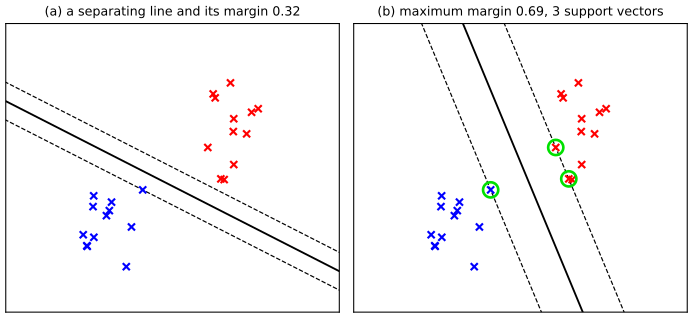
fig7_1. Download: PDF · SVGResult 7.1 (canonical form; Exercise 7.2) pp. 327–328, (7.4)–(7.6)
(a) The objective of (7.3) is unchanged by \((\mathbf{w},b)\to(\kappa\mathbf{w},\kappa b)\), \(\kappa\gt0\). Hence (7.3) is equivalent to the quadratic programme
\[ \operatorname*{arg\,min}_{\mathbf{w},b}\ \frac12\|\mathbf{w}\|^2\quad\text{subject to}\quad t_n(\mathbf{w}^\T\bm\phi(\mathbf{x}_n)+b)\ge1,\ n=1,\dots,N, \tag{7.5, 7.6} \]whose solution has margin \(\rho=1/\|\mathbf{w}\|\). (b) The solution \((\mathbf{w},b)\) is unique, and at least one constraint of each class is active (an equality). (c) Replacing the \(1\) in the constraints by any \(\gamma\gt0\) gives \(\gamma(\mathbf{w},b)\): the same hyperplane.
Proof
(a) Scaling multiplies numerator and denominator of the objective in (7.3) by \(\kappa\). Let \(\rho^\star\) be the optimal value of (7.3), over the \((\mathbf{w},b)\) with \(t_ny_n\gt0\) for all \(n\). Take any \((\mathbf{w},b)\) feasible for (7.5), i.e. with \(\min_nt_ny_n\ge1\). Then \(1/\|\mathbf{w}\|\)
(b) The feasible set of (7.5) is closed, convex and (by separability and rescaling) nonempty, and \(\frac12\|\mathbf{w}\|^2\) is strictly convex and coercive in \(\mathbf{w}\), so the optimal \(\mathbf{w}\) exists and is unique. Take an optimal \((\mathbf{w},b)\). Active constraints in both classes. Suppose no positive point is active, i.e. \(y_n\gt1\) for all \(t_n=+1\). Lower \(b\) by a small \(\delta\gt0\): the positive constraints stay strict, and the negative ones (\(-y_n\ge1\)) become looser, so now every constraint is strict. Then \((1-\varepsilon)\mathbf{w}\) with small \(\varepsilon\) is still feasible (finitely many strict inequalities) and has smaller norm, contradicting optimality. The same argument with \(b\) raised excludes the case of no active negative point. Uniqueness of \(b\). With an active positive point \(n\) we have \(\mathbf{w}^\T\bm\phi_n+b=1\), so \(b=1-\mathbf{w}^\T\bm\phi_n\) is determined by the unique \(\mathbf{w}\).
(c) If \(t_ny_n\ge\gamma\) then \(t_n(y_n/\gamma)\ge1\); so \((\mathbf{w},b)\) is feasible for the \(\gamma\)-problem iff \((\mathbf{w}/\gamma,b/\gamma)\) is feasible for (7.5). The objective of the \(\gamma\)-problem is \(\frac12\|\mathbf{w}\|^2\)
The bias \(b\) seems to have dropped out of the objective (7.6); it is determined implicitly through the constraints. To solve the problem, attach a multiplier \(a_n\ge0\) to each constraint (toolkit: Lagrange multipliers), with a minus sign because we minimise over \((\mathbf{w},b)\):
\[ L(\mathbf{w},b,\mathbf{a})=\frac12\|\mathbf{w}\|^2-\sum_{n=1}^{N}a_n\big\{t_n(\mathbf{w}^\T\bm\phi(\mathbf{x}_n)+b)-1\big\}. \tag{7.7} \]Result 7.2 (the dual problem) pp. 328–329, (7.8)–(7.13)
Setting \(\partial L/\partial\mathbf{w}=\mathbf{0}\) and \(\partial L/\partial b=0\) gives
\[ \mathbf{w}=\sum_{n=1}^{N}a_nt_n\bm\phi(\mathbf{x}_n),\tag{7.8} \] \[ 0=\sum_{n=1}^{N}a_nt_n.\tag{7.9} \]Eliminating \(\mathbf{w}\) and \(b\) leaves the dual: maximise
\[ \widetilde L(\mathbf{a})=\sum_{n=1}^{N}a_n-\frac12\sum_{n=1}^{N}\sum_{m=1}^{N}a_na_mt_nt_mk(\mathbf{x}_n,\mathbf{x}_m)\tag{7.10} \]subject to
\[ a_n\ge0,\ n=1,\dots,N,\tag{7.11} \] \[ \sum_{n=1}^{N}a_nt_n=0,\tag{7.12} \]with \(k(\mathbf{x},\mathbf{x}')\)
Proof
Stationarity. \(\nabla_{\mathbf{w}}L\)
Why (7.12) appears. For fixed \(\mathbf{a}\ge\mathbf{0}\), \(L\) is a convex function of \((\mathbf{w},b)\), linear in \(b\) with slope \(-\sum_na_nt_n\). If that slope is nonzero, \(\inf_bL=-\infty\), so the dual function \(g(\mathbf{a})=\inf_{\mathbf{w},b}L\) is finite only on the set (7.12); there the infimum is attained at (7.8).
Substitution. Insert (7.8) and use (7.9) so that the \(b\) term vanishes:
\[ \tfrac12\|\mathbf{w}\|^2=\tfrac12\sum_{n,m}a_na_mt_nt_m\bm\phi_n^\T\bm\phi_m,\qquad \sum_na_nt_n\mathbf{w}^\T\bm\phi_n=\sum_{n,m}a_na_mt_nt_m\bm\phi_m^\T\bm\phi_n,\qquad b\sum_na_nt_n=0. \]Therefore \(L=\frac12Q-Q-0+\sum_na_n\) with \(Q=\sum_{n,m}a_na_mt_nt_mk_{nm}\), i.e. (7.10). Substituting (7.8) into (7.1) gives (7.13).
Concavity and the role of positive definiteness. \(Q=\|\sum_na_nt_n\bm\phi_n\|^2\ge0\), i.e. the matrix \(t_nt_mk_{nm}\) is positive semidefinite whenever \(k\) is a valid kernel (Chapter 6); so \(\widetilde L\) is concave and any local maximum is global, and \(\widetilde L\le\sum_na_n\) is bounded above on each bounded set of \(\mathbf{a}\). For an indefinite \(k\), \(Q\) could be negative along some feasible direction, and the dual could be unbounded, which is the role of "positive definite" in the book's remark.
No duality gap. The primal is a convex quadratic problem with affine constraints, which is feasible by separability; for such problems strong duality holds (the Slater condition is only needed for nonlinear constraints), so the dual maximum equals the primal minimum. ∎
The primal has \(M\) variables (the dimension of feature space) and the dual has \(N\); with fixed \(M\lt N\) the dual looks worse, but it needs only the kernel, so \(\bm\phi\) may be infinite dimensional. Note also that (7.8) is a representer theorem for this problem: \(\mathbf{w}\) lies in the span of the training features.
Result 7.3 (KKT conditions and support vectors) p. 330, (7.14)–(7.16)
At the solution, for every \(n\)
\[ a_n\ge0,\tag{7.14} \] \[ t_ny(\mathbf{x}_n)-1\ge0,\tag{7.15} \] \[ a_n\{t_ny(\mathbf{x}_n)-1\}=0.\tag{7.16} \]So either \(a_n=0\), and the point does not appear in (7.13), or \(t_ny(\mathbf{x}_n)=1\), and the point lies on a margin hyperplane. The points with \(a_n\gt0\) are the support vectors, \(\mathcal{S}=\{n:a_n\gt0\}\).
Derivation of the KKT conditions
(7.14) is dual feasibility and (7.15) is primal feasibility (7.5). For (7.16) (complementary slackness) let \((\mathbf{w}^\star,b^\star)\) be primal optimal and \(\mathbf{a}^\star\) dual optimal. Strong duality (Result 7.2) gives \(\frac12\|\mathbf{w}^\star\|^2\)
the last step because each \(a_n^\star\ge0\) and \(t_ny_n^\star-1\ge0\). Both ends are equal, so \(\sum_na_n^\star\{t_ny_n^\star-1\}=0\); a sum of nonnegative terms is zero only if every term is zero, which is (7.16). ∎
This is the central practical fact: once trained, only the support vectors are kept. Geometrically they are the points on the two margin hyperplanes (Figure 7.1), and the other points can be moved around freely, as long as they stay outside the margin, without changing the solution. The bias follows from any support vector.
Result 7.4 (the bias) p. 330, (7.17)–(7.18)
For every support vector, \(t_n\big(\sum_{m\in\mathcal{S}}a_mt_mk(\mathbf{x}_n,\mathbf{x}_m)+b\big)\)
Derivation
(7.17) is (7.16) with \(a_n\gt0\) and (7.13) (the sum over all \(m\) reduces to \(m\in\mathcal{S}\) because \(a_m=0\) otherwise). Multiply (7.17) by \(t_n\) and use \(t_n^2=1\): \(\sum_ma_mt_mk_{nm}+b=t_n\), i.e. \(b=t_n-\sum_{m\in\mathcal{S}}a_mt_mk_{nm}\) for each \(n\in\mathcal{S}\). Each is an exact solution; averaging them gives (7.18). The average is preferred because \(a_n\) and the kernel values are known only to the accuracy of the quadratic-programming solver, and the average reduces the error of a single noisy equation. ∎
The maximum margin classifier is also a regularised error minimisation,
\[ \sum_{n=1}^{N}E_\infty\big(y(\mathbf{x}_n)t_n-1\big)+\lambda\|\mathbf{w}\|^2,\tag{7.19} \]where \(E_\infty(z)=0\) for \(z\ge0\) and \(+\infty\) otherwise. The infinite penalty enforces (7.5), and any \(\lambda\gt0\) gives the same minimiser, so its value is irrelevant.
Result 7.5 (the margin from the dual solution; Exercises 7.4 and 7.5) p. 357, (7.123)–(7.125)
If \(\rho=1/\|\mathbf{w}\|\) is the margin and \(\mathbf{a}\) maximises (7.10) under (7.11), (7.12), then
\[ \frac1{\rho^2}=\|\mathbf{w}\|^2=\sum_{n=1}^{N}a_n=2\widetilde L(\mathbf{a}).\tag{7.123, 7.124, 7.125} \]Proof
\(\rho=1/\|\mathbf{w}\|\) is (7.4) with the closest point at distance \(t_ny_n/\|\mathbf{w}\|=1/\|\mathbf{w}\|\); so \(\rho^{-2}=\|\mathbf{w}\|^2\), which is (7.125). Next, by (7.8), then \(\bm\phi_n^\T\mathbf{w}=y_n-b\), then (7.9),
\[ \|\mathbf{w}\|^2=\sum_na_nt_n\mathbf{w}^\T\bm\phi_n=\sum_na_nt_n(y_n-b)=\sum_na_nt_ny_n-b\sum_na_nt_n=\sum_na_nt_ny_n. \]By (7.16), \(a_nt_ny_n=a_n\) for every \(n\) (if \(a_n=0\) both sides vanish; otherwise \(t_ny_n=1\)). So \(\|\mathbf{w}\|^2=\sum_na_n\), which is (7.123). Finally the second term of (7.10) is \(\frac12\|\mathbf{w}\|^2\) by (7.8), so \(\widetilde L\)
Filling the gap 7.2: the feature space of a kernel can be huge, yet the data live on a small manifold p. 336, (7.42)
For \(\mathbf{x},\mathbf{z}\in\mathbb{R}^2\),
Verification
\[ k(\mathbf{x},\mathbf{z})=(1+\mathbf{x}^\T\mathbf{z})^2=1+2x_1z_1+2x_2z_2+x_1^2z_1^2+2x_1z_1x_2z_2+x_2^2z_2^2=\bm\phi(\mathbf{x})^\T\bm\phi(\mathbf{z}), \tag{7.42} \]with \(\bm\phi(\mathbf{x})\)
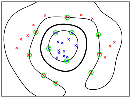
fig7_2. Download: PDF · SVG7.1.1 Overlapping class distributions
pp. 331–336 If the classes overlap in feature space, exact separation does not exist (and, if it did, would generalise poorly). Introduce one slack variable \(\xi_n\ge0\) per training point: \(\xi_n=0\) on or inside the correct margin boundary and \(\xi_n=|t_n-y(\mathbf{x}_n)|\) otherwise. A point on the decision surface has \(\xi_n=1\), a misclassified one \(\xi_n\gt1\) (Figure 7.3). The constraints (7.5) become
\[ t_ny(\mathbf{x}_n)\ge1-\xi_n,\qquad \xi_n\ge0.\tag{7.20} \]We minimise
\[ C\sum_{n=1}^{N}\xi_n+\frac12\|\mathbf{w}\|^2,\tag{7.21} \]where \(C\gt0\) trades margin against slack. Since a misclassified point has \(\xi_n\gt1\), \(\sum_n\xi_n\) bounds the number of training errors from above; \(C\to\infty\) recovers the hard-margin machine. Slack grows linearly with the distance past the margin, so the machine is still sensitive to outliers.
Result 7.6 (the soft-margin dual and its KKT conditions) pp. 332–334, (7.22)–(7.37)
The Lagrangian, with multipliers \(a_n\ge0\) for (7.20) and \(\mu_n\ge0\) for \(\xi_n\ge0\), is
\[ L(\mathbf{w},b,\bm\xi,\mathbf{a},\bm\mu)=\frac12\|\mathbf{w}\|^2+C\sum_n\xi_n-\sum_na_n\{t_ny(\mathbf{x}_n)-1+\xi_n\}-\sum_n\mu_n\xi_n.\tag{7.22} \]Erratum. The book prints \(L(\mathbf{w},b,\mathbf{a})\) on the left; it depends on \(\bm\xi\) and \(\bm\mu\) as well.
The KKT conditions are, for \(n=1,\dots,N\),
\[ \begin{aligned}a_n&\ge0, &(7.23)\\ t_ny(\mathbf{x}_n)-1+\xi_n&\ge0, &(7.24)\\ a_n(t_ny(\mathbf{x}_n)-1+\xi_n)&=0, &(7.25)\\ \mu_n&\ge0, &(7.26)\\ \xi_n&\ge0, &(7.27)\\ \mu_n\xi_n&=0. &(7.28)\end{aligned} \]Stationarity gives
\[ \mathbf{w}=\sum_na_nt_n\bm\phi(\mathbf{x}_n),\tag{7.29} \] \[ \sum_na_nt_n=0,\tag{7.30} \] \[ a_n=C-\mu_n,\tag{7.31} \]and the dual is to maximise
\[ \widetilde L(\mathbf{a})=\sum_na_n-\frac12\sum_{n,m}a_na_mt_nt_mk(\mathbf{x}_n,\mathbf{x}_m)\tag{7.32} \]subject to the box constraints and the balance condition
\[ 0\le a_n\le C,\tag{7.33} \] \[ \sum_na_nt_n=0.\tag{7.34} \]Predictions are again (7.13). Cases at the solution:
| multiplier | slack | position of \(\mathbf{x}_n\) |
|---|---|---|
| \(a_n=0\) | \(\xi_n=0\) | correct side of, or on, the margin boundary; not a support vector |
| \(0\lt a_n\lt C\) | \(\xi_n=0\) | exactly on the margin: \(t_ny_n=1\) |
| \(a_n=C\) | \(\xi_n\ge0\) | on or inside the margin (\(\xi_n\le1\), correctly classified) or misclassified (\(\xi_n\gt1\)) |
For a support vector \(t_ny(\mathbf{x}_n)=1-\xi_n\) (7.35). For the unbounded ones (\(0\lt a_n\lt C\)) the bias satisfies (7.36), and the stable average is
\[ b=\frac1{N_{\mathcal{M}}}\sum_{n\in\mathcal{M}}\Big(t_n-\sum_{m\in\mathcal{S}}a_mt_mk(\mathbf{x}_n,\mathbf{x}_m)\Big),\tag{7.37} \]\(\mathcal{M}=\{n:0\lt a_n\lt C\}\), \(N_{\mathcal{M}}=|\mathcal{M}|\).
Derivation
Stationarity. \(\nabla_{\mathbf{w}}L\)
The dual. Substitute (7.31) into (7.22): the slack terms combine as \(\xi_n(C-a_n-\mu_n)=0\), so all \(\xi\)-dependence cancels and \(L=\frac12\|\mathbf{w}\|^2-\sum_na_n(t_ny_n-1)\), exactly the separable-case expression. Then (7.29) and (7.30) reduce it to (7.32) as in Result 7.2.
The box. \(a_n\ge0\) is (7.23); \(\mu_n\ge0\) and (7.31) give \(a_n=C-\mu_n\le C\). (The dual is a maximisation of (7.32); the book's sentence above (7.33) says "minimize", which the errata correct.)
The cases. If \(a_n\gt0\), (7.25) forces \(t_ny_n=1-\xi_n\) (7.35). If \(a_n\lt C\), (7.31) gives \(\mu_n=C-a_n\gt0\), and (7.28) forces \(\xi_n=0\), so \(t_ny_n=1\). If \(a_n=C\), then \(\mu_n=0\) and (7.28) puts no restriction on \(\xi_n\): any \(\xi_n\ge0\) is allowed, subject to (7.35). If \(a_n=0\), then \(\mu_n=C\gt0\) so \(\xi_n=0\) and (7.24) gives \(t_ny_n\ge1\).
Bias. For \(n\in\mathcal{M}\), \(\xi_n=0\) and \(a_n\gt0\) so \(t_ny_n=1\), which is (7.36); multiplying by \(t_n\) and averaging as in Result 7.4 gives (7.37) (only unbounded multipliers can be used, since for \(a_n=C\) the slack is unknown). ∎
The parameter \(C\) is like an inverse regularisation constant. The ν-SVM replaces it by a parameter with a direct meaning.
Result 7.7 (the ν-SVM) pp. 334–335, (7.38)–(7.41)
Consider the primal problem: minimise \(\frac12\|\mathbf{w}\|^2-\nu\rho\)
subject to
\[ 0\le a_n\le1/N,\tag{7.39} \] \[ \sum_na_nt_n=0,\tag{7.40} \] \[ \sum_na_n\ge\nu.\tag{7.41} \]At the solution (with \(\rho\gt0\)), \(\sum_na_n=\nu\), the fraction of margin errors (\(\xi_n\gt0\)) is at most \(\nu\), and the fraction of support vectors is at least \(\nu\). The solution coincides with the C-SVM solution for \(C=1/(N\rho)\).
Derivation
Lagrangian. With multipliers \(a_n\), \(\mu_n\), \(\delta\ge0\),
\[ L=\tfrac12\|\mathbf{w}\|^2-\nu\rho+\tfrac1N\sum_n\xi_n-\sum_na_n\{t_ny_n-\rho+\xi_n\}-\sum_n\mu_n\xi_n-\delta\rho. \]Stationarity: \(\mathbf{w}=\sum_na_nt_n\bm\phi_n\); \(\sum_na_nt_n=0\); \(a_n+\mu_n=1/N\), so \(0\le a_n\le1/N\); and \(\partial L/\partial\rho=-\nu+\sum_na_n-\delta=0\), so \(\sum_na_n=\nu+\delta\ge\nu\), which is (7.41).
Dual. Substituting, the \(\xi\) terms cancel by \(a_n+\mu_n=1/N\), the \(\rho\) terms by the last equation, and the \(b\) term by the balance condition, leaving \(\frac12\|\mathbf{w}\|^2\)
The bounds. If \(\rho\gt0\) then \(\delta=0\) (complementary slackness for \(\delta\rho=0\)), so \(\sum_na_n=\nu\). A point with \(\xi_n\gt0\) has \(\mu_n=0\) (since \(\mu_n\xi_n=0\)), hence \(a_n=1/N\); thus \(\#\{\xi_n\gt0\}/N\le\sum_na_n=\nu\). Every \(a_n\) is at most \(1/N\), so \(\nu=\sum_na_n\le\#\{a_n\gt0\}/N\): at least a fraction \(\nu\) are support vectors.
Link to \(C\). Rescale \(\tilde{\mathbf{w}}=\mathbf{w}/\rho\), \(\tilde b=b/\rho\), \(\tilde\xi_n=\xi_n/\rho\), so that \(t_n\tilde y_n\ge1-\tilde\xi_n\). The objective becomes \(\rho^2\big[\frac12\|\tilde{\mathbf{w}}\|^2+\frac1{N\rho}\sum_n\tilde\xi_n\big]\)
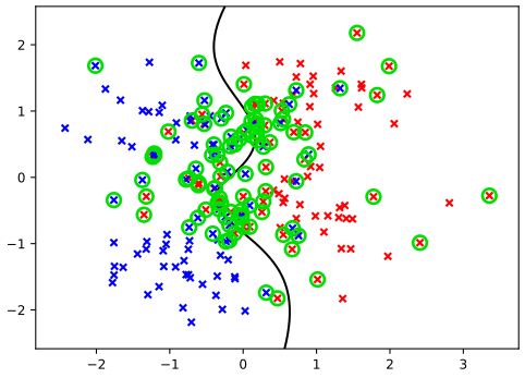
fig7_4. Download: PDF · SVGAlgorithm 7.1 (training: from chunking to SMO) pp. 334–335
The dual objective is quadratic and concave and the constraints are linear, so every local optimum is global. But the kernel matrix has \(N^2\) entries, so a generic QP solver is too costly for large \(N\). Three ideas, in order of increasing decomposition:
- Chunking (Vapnik, 1982): the value of (7.32) is unchanged if the rows and columns of \(\mathbf{K}\) belonging to \(a_n=0\) are deleted, so solve a QP on a working set and keep adding violators of the KKT conditions until every point satisfies them.
- Decomposition (Osuna et al., 1996): solve a sequence of QPs of fixed size, so memory is bounded whatever \(N\) is.
- Sequential minimal optimisation (Platt, 1999): the extreme case of two multipliers at a time. Since (7.34) ties them, the subproblem is a one-dimensional quadratic with a closed-form solution (Filling the gap 7.3). Repeat: pick a pair that violates the KKT conditions (heuristics choose the pair), update both analytically, until all points satisfy the KKT conditions within a tolerance. Empirically the cost scales between linear and quadratic in \(N\).
Filling the gap 7.3: the analytic two-multiplier step of SMO p. 335
The book says the two-multiplier subproblem "can be solved analytically". Here it is for the soft-margin dual (7.32)–(7.34).
Derivation
Fix all multipliers except \(a_i\) and \(a_j\). By (7.34) \(t_ia_i+t_ja_j=\zeta\) stays constant, so a move is \(a_j\to a_j+\delta\), \(a_i\to a_i-t_it_j\delta\) (check: \(t_i(-t_it_j\delta)+t_j\delta\)
The derivative along the move is therefore
\[ \frac{dW}{d\delta}=\frac{\partial W}{\partial a_j}-t_it_j\frac{\partial W}{\partial a_i}=(-t_jE_j+t_jb)-t_it_j(-t_iE_i+t_ib)=t_j(E_i-E_j). \]The objective is quadratic along the line. Its second derivative is \(-\mathbf{v}^\T(\mathbf{T}\mathbf{K}\mathbf{T})\mathbf{v}\), with \(\mathbf{T}=\diag(t)\) and \(\mathbf{v}=\mathbf{e}_j-t_it_j\mathbf{e}_i\), and \(\mathbf{T}\mathbf{v}\)
The clipping interval comes from the box (7.33) for both multipliers: if \(t_i\ne t_j\), \(L_b=\max(0,a_j-a_i)\) and \(H_b=\min(C,C+a_j-a_i)\); if \(t_i=t_j\), \(L_b=\max(0,a_i+a_j-C)\) and \(H_b=\min(C,a_i+a_j)\). (If \(\eta=0\), the objective is linear along the line and the maximum is at an end of the interval.) After the step \(b\) is recomputed from a multiplier strictly inside \((0,C)\). Each step does not decrease \(W\), and an exactly solved subproblem needs no matrix inversion. ∎
Two further remarks of the book. (i) The SVM outputs a decision, not a probability. Platt scaling fits a sigmoid to the machine's outputs,
\[ p(t=1\given\mathbf{x})=\sigma(Ay(\mathbf{x})+B),\tag{7.43} \]by minimising the cross-entropy on data held out from the SVM training (otherwise the outputs are over-confident because the training points sit at \(|y|\ge1\) by construction); this assumes \(y\) is a log-odds, which SVM training does not encourage, so the fit can be a poor approximation of the posterior (Tipping, 2001). Veropoulos et al. (1999) control the false positive/negative trade-off by using different box sizes \(C_+\), \(C_-\) for the two classes. (ii) Tong and Koller (2000) show that a hybrid of generative and discriminative models gives the maximum margin hyperplane in the limit where the Parzen width \(\sigma^2\to0\), because the hyperplane is then dominated by the nearest points.
7.1.2 Relation to logistic regression
pp. 336–338 The soft-margin machine is also a regularised error minimisation, which makes the comparison with logistic regression (Section 4.3.2) transparent.
Result 7.8 (the SVM as hinge-loss regularisation; Exercise 7.6) pp. 336–338, (7.44)–(7.48)
Minimising (7.21) over \((\mathbf{w},b,\bm\xi)\) subject to (7.20) is the same as minimising, over \((\mathbf{w},b)\),
\[ \sum_{n=1}^{N}E_{\rm SV}(y_nt_n)+\lambda\|\mathbf{w}\|^2,\qquad\lambda=(2C)^{-1},\tag{7.44} \] \[ E_{\rm SV}(yt)=[1-yt]_+\tag{7.45} \](the hinge loss). With \(t\in\{-1,1\}\), logistic regression has \(p(t\given y)=\sigma(yt)\) (7.46), and its regularised negative log likelihood is
\[ \sum_{n=1}^{N}E_{\rm LR}(y_nt_n)+\lambda\|\mathbf{w}\|^2,\qquad E_{\rm LR}(yt)=\ln(1+e^{-yt}).\tag{7.47, 7.48} \]Proof
Hinge. For fixed \((\mathbf{w},b)\), the constraints (7.20) say \(\xi_n\ge\max(0,1-t_ny_n)\) and \(\xi_n\) enters (7.21) with positive coefficient \(C\), so the best \(\xi_n\) is the smallest allowed one: \(\xi_n=[1-y_nt_n]_+\) (zero when \(y_nt_n\ge1\), and \(1-y_nt_n\) otherwise). Substituting, (7.21) becomes \(C\sum_n[1-y_nt_n]_++\frac12\|\mathbf{w}\|^2\)
Logistic. If \(p(t=1\given y)=\sigma(y)\) then \(p(t=-1\given y)=1-\sigma(y)=\sigma(-y)\) (symmetry of the sigmoid), so both cases are \(\sigma(yt)\). The negative log likelihood of independent data is \(-\sum_n\ln\sigma(y_nt_n)\)
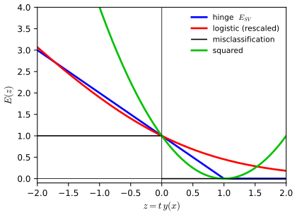
fig7_5. Download: PDF · SVGBoth are continuous (convex) upper-bound surrogates of the 0/1 error. The key difference: the hinge is exactly zero for \(yt\ge1\) (the flat region), so correctly classified points beyond the margin have zero loss and zero gradient and drop out of the solution (\(a_n=0\)); the logistic loss is never zero, so every point keeps a nonzero weight \(\sigma(-y_nt_n)\) in the gradient and the solution is not sparse. The squared error \((yt-1)^2\) punishes points that are far on the correct side, which makes no sense for classification.
Filling the gap 7.4: why the SVM gives no probabilities p. 331
Which function does each loss ideally estimate? Let \(p=P(t=1\given\mathbf{x})\) and minimise the pointwise expected loss over the value \(y\).
Derivation
Logistic loss. \(R(y)=p\ln(1+e^{-y})+(1-p)\ln(1+e^{y})\). Using \(\frac{d}{dy}\ln(1+e^{-y})=-\sigma(-y)\) and \(\frac{d}{dy}\ln(1+e^{y})=\sigma(y)\),
\[ R'(y)=-p\sigma(-y)+(1-p)\sigma(y)=\sigma(y)-p \]It is zero at \(y=\ln\frac p{1-p}\): the minimiser is the log-odds, so \(\sigma(y)\) estimates the posterior.
Hinge loss. \(R(y)=p[1-y]_++(1-p)[1+y]_+\). For \(|y|\le1\) this equals \(p(1-y)+(1-p)(1+y)=1+(1-2p)y\), linear in \(y\) with slope \(1-2p\). For \(y\gt1\) it equals \((1-p)(1+y)\), increasing, and for \(y\lt-1\) it equals \(p(1-y)\), decreasing. So the minimum is at \(y=+1\) if \(p\gt\frac12\) and \(y=-1\) if \(p\lt\frac12\): the hinge minimiser is \(\operatorname{sign}(2p-1)\), which gives the Bayes classifier but throws away the value of \(p\). ∎
7.1.3 Multiclass SVMs
pp. 338–339 The SVM is a two-class machine. The common recipes for \(K\) classes:
- One-versus-the-rest (Vapnik, 1998): \(K\) machines \(y_k\), the \(k\)th trained with class \(k\) as positive and the rest as negative; predict \(\arg\max_ky_k(\mathbf{x})\) (7.49). Problems: the \(y_k\) are trained on different tasks and need not be on a common scale; the training sets are imbalanced (with ten equal classes, 90% negatives); the plain sign rule can assign an input to several classes or none (Figure 4.2). Lee et al. (2001) set the negative target to \(-1/(K-1)\) to restore a symmetry.
- All-in-one (Weston and Watkins, 1999): one optimisation of size \((K-1)N\) instead of \(K\) problems of size \(N\); the cost goes from \(O(KN^2)\) to \(O(K^2N^2)\).
- One-versus-one: \(K(K-1)/2\) machines, one per pair, and a vote. Each machine sees only two classes' data, so the total training cost can be small, but for large \(K\) it needs many machines and ties are possible. The DAGSVM (Platt et al., 2000) arranges the pairwise machines in a directed acyclic graph so that a test point needs only \(K-1\) evaluations.
- Error-correcting output codes (Dietterich and Bakiri, 1995; Allwein et al., 2000): each class gets a binary code word, one binary machine per code bit, and a new point is assigned to the nearest code word. One-versus-one voting is a special case; the redundancy corrects some wrong outputs.
In practice one-versus-the-rest is most used, in spite of its ad hoc nature. The RVM (Section 7.2.3) has a principled multiclass form through the softmax.
Filling the gap 7.5: single-class SVMs, two formulations that coincide p. 339
The book states that for kernels that depend only on \(\mathbf{x}-\mathbf{x}'\) the algorithms of Schölkopf et al. (2001) (separate all but a fraction \(\nu\) of the data from the origin by a hyperplane) and Tax and Duin (1999) (smallest sphere containing all but a fraction \(\nu\)) are equivalent. Here is why.
Derivation
If \(k(\mathbf{x},\mathbf{x}')\)
7.1.4 SVMs for regression
pp. 339–343 Regularised least squares minimises \(\frac12\sum_n(y_n-t_n)^2\)
and minimise, with the convention that the factor \(C\) multiplies the error,
\[ C\sum_{n=1}^{N}E_\epsilon(y(\mathbf{x}_n)-t_n)+\frac12\|\mathbf{w}\|^2.\tag{7.52} \]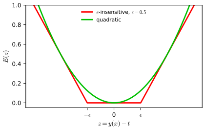
fig7_6. Download: PDF · SVGAs before, introduce two slack variables per point: \(\xi_n\ge0\) if \(t_n\) lies above the tube and \(\hat\xi_n\ge0\) if below (Figure 7.7), with
\[ t_n\le y(\mathbf{x}_n)+\epsilon+\xi_n,\tag{7.53} \] \[ t_n\ge y(\mathbf{x}_n)-\epsilon-\hat\xi_n,\tag{7.54} \]and minimise
\[ C\sum_{n=1}^{N}(\xi_n+\hat\xi_n)+\frac12\|\mathbf{w}\|^2.\tag{7.55} \]At the optimum \(\xi_n+\hat\xi_n=E_\epsilon(y_n-t_n)\) (the same argument as for the hinge: each slack takes its smallest allowed value, and a point cannot be both above and below the tube), so (7.55) is (7.52).
Result 7.9 (the SVM regression dual; Exercises 7.7 and 7.8) pp. 341–343, (7.56)–(7.69)
With multipliers \(a_n,\hat a_n\ge0\) for (7.53), (7.54) and \(\mu_n,\hat\mu_n\ge0\) for the slack constraints, the Lagrangian is
\[ \begin{aligned}L=\;&C\sum_n(\xi_n+\hat\xi_n)+\tfrac12\|\mathbf{w}\|^2-\sum_n(\mu_n\xi_n+\hat\mu_n\hat\xi_n)\\&-\sum_na_n(\epsilon+\xi_n+y_n-t_n)-\sum_n\hat a_n(\epsilon+\hat\xi_n-y_n+t_n).\end{aligned}\tag{7.56} \]Stationarity gives
\[ \mathbf{w}=\sum_n(a_n-\hat a_n)\bm\phi(\mathbf{x}_n),\tag{7.57} \] \[ \sum_n(a_n-\hat a_n)=0,\tag{7.58} \] \[ a_n+\mu_n=C,\tag{7.59} \] \[ \hat a_n+\hat\mu_n=C.\tag{7.60} \]The dual is to maximise
\[ \widetilde L(\mathbf{a},\hat{\mathbf{a}})=-\frac12\sum_{n,m}(a_n-\hat a_n)(a_m-\hat a_m)k(\mathbf{x}_n,\mathbf{x}_m)-\epsilon\sum_n(a_n+\hat a_n)+\sum_n(a_n-\hat a_n)t_n\tag{7.61} \]subject to
\[ 0\le a_n\le C,\tag{7.62} \] \[ 0\le\hat a_n\le C\tag{7.63} \]and (7.58). Predictions are
\[ y(\mathbf{x})=\sum_n(a_n-\hat a_n)k(\mathbf{x},\mathbf{x}_n)+b.\tag{7.64} \]The KKT conditions are
\[ \begin{aligned}a_n(\epsilon+\xi_n+y_n-t_n)&=0, &(7.65)\\ \hat a_n(\epsilon+\hat\xi_n-y_n+t_n)&=0, &(7.66)\\ (C-a_n)\xi_n&=0, &(7.67)\\ (C-\hat a_n)\hat\xi_n&=0. &(7.68)\end{aligned} \]Consequences: (i) \(\xi_n\gt0\Rightarrow a_n=C\) and \(\hat\xi_n\gt0\Rightarrow\hat a_n=C\) (Exercise 7.8); (ii) for every \(n\), \(a_n\hat a_n=0\); (iii) the support vectors are the points with \(a_n\ne0\) or \(\hat a_n\ne0\), exactly those on or outside the tube; points strictly inside have \(a_n=\hat a_n=0\); (iv) the bias, from any \(n\) with \(0\lt a_n\lt C\) (then \(\xi_n=0\) and \(\epsilon+y_n-t_n=0\)), is
\[ b=t_n-\epsilon-\mathbf{w}^\T\bm\phi(\mathbf{x}_n)=t_n-\epsilon-\sum_m(a_m-\hat a_m)k(\mathbf{x}_n,\mathbf{x}_m);\tag{7.69} \]similarly \(b=t_n+\epsilon-\sum_m(a_m-\hat a_m)k_{nm}\) for any \(n\) with \(0\lt\hat a_n\lt C\). In practice average over all such estimates.
Derivation
Stationarity. Substitute \(y_n=\mathbf{w}^\T\bm\phi_n+b\). \(\nabla_{\mathbf{w}}L\)
The dual (Exercise 7.7). The \(\xi_n\) terms of (7.56) are \(\xi_n(C-\mu_n-a_n)=0\) and similarly for \(\hat\xi_n\), so they vanish. What remains is
\[ L=\tfrac12\|\mathbf{w}\|^2-\epsilon\sum_n(a_n+\hat a_n)+\sum_n(a_n-\hat a_n)t_n-\sum_n(a_n-\hat a_n)y_n. \]Now \(\sum_n(a_n-\hat a_n)y_n\)
Constraints. \(a_n\ge0\) and \(\mu_n\ge0\) with (7.59) give \(0\le a_n\le C\), likewise (7.63); (7.58) stays. Substituting (7.57) in (7.1) gives (7.64).
KKT consequences. (7.65)–(7.66) are complementary slackness for (7.53), (7.54); (7.67)–(7.68) are \(\mu_n\xi_n=0\), \(\hat\mu_n\hat\xi_n=0\) rewritten with (7.59), (7.60). (i) If \(\xi_n\gt0\), (7.67) forces \(C-a_n=0\). (ii) If both \(a_n\gt0\) and \(\hat a_n\gt0\), (7.65) and (7.66) give \(\epsilon+\xi_n+y_n-t_n=0\) and \(\epsilon+\hat\xi_n-y_n+t_n=0\); adding gives \(2\epsilon+\xi_n+\hat\xi_n=0\), impossible since \(\epsilon\gt0\) and the slacks are \(\ge0\). (iii) \(a_n\ne0\) needs \(\epsilon+\xi_n+y_n-t_n=0\), i.e. \(t_n=y_n+\epsilon+\xi_n\ge y_n+\epsilon\): on or above the upper edge of the tube; likewise for \(\hat a_n\) below the lower edge. For \(|t_n-y_n|\lt\epsilon\) neither equation can hold with nonnegative slack, so both multipliers vanish. (iv) For \(0\lt a_n\lt C\), (7.67) gives \(\xi_n=0\), then (7.65) gives \(\epsilon+y_n-t_n=0\), and (7.1) with (7.57) gives (7.69). ∎
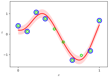
fig7_8. Download: PDF · SVGResult 7.10 (ν-SVM for regression) p. 343, (7.70)–(7.74)
Fix a fraction \(\nu\) instead of the width \(\epsilon\): minimise \(\frac12\|\mathbf{w}\|^2\)
subject to
\[ 0\le a_n\le C/N,\tag{7.71} \] \[ 0\le\hat a_n\le C/N,\tag{7.72} \] \[ \sum_n(a_n-\hat a_n)=0,\tag{7.73} \] \[ \sum_n(a_n+\hat a_n)\le\nu C.\tag{7.74} \]At most \(\nu N\) points lie outside the tube and at least \(\nu N\) are support vectors.
Derivation
Add a multiplier \(\delta\ge0\) for \(\epsilon\ge0\). The terms in \(\epsilon\) in the Lagrangian are \(C\nu\epsilon-\epsilon\sum_n(a_n+\hat a_n)\)
7.1.5 Computational learning theory
pp. 344–345 SVMs were originally motivated by statistical (computational) learning theory. In the PAC (probably approximately correct) framework of Valiant (1984), the data \(\mathcal{D}\) of size \(N\) are drawn from \(p(\mathbf{x},t)\) with labels from an unknown function \(t=g(\mathbf{x})\), and a learned function \(f(\mathbf{x};\mathcal{D})\) from a class \(\mathcal{F}\) has good generalisation if
\[ \mathbb{E}_{\mathbf{x},t}\big[\mathbb{I}(f(\mathbf{x};\mathcal{D})\ne t)\big]\lt\epsilon\tag{7.75} \]with probability at least \(1-\delta\) over \(\mathcal{D}\). The theory asks how large \(N\) must be as a function of \(\epsilon\), \(\delta\) and the complexity of \(\mathcal{F}\).
Result 7.11 (sample size for a finite class; the idea behind PAC bounds)
Let \(\mathcal{F}\) be finite and suppose the target is in \(\mathcal{F}\). If \(f\in\mathcal{F}\) is consistent with the \(N\) training examples, then with probability at least \(1-\delta\) its error is below \(\epsilon\) provided
\[ N\ge\frac1\epsilon\Big(\ln|\mathcal{F}|+\ln\frac1\delta\Big). \]Proof
A fixed function with true error at least \(\epsilon\) classifies one random example correctly with probability at most \(1-\epsilon\), hence all \(N\) independent examples with probability at most \((1-\epsilon)^N\le e^{-\epsilon N}\). By the union bound, the probability that some function in \(\mathcal{F}\) with error at least \(\epsilon\) is consistent with the data is at most \(|\mathcal{F}|e^{-\epsilon N}\). Requiring this to be at most \(\delta\) gives the condition. ∎
For infinite classes \(\ln|\mathcal{F}|\) is replaced by the Vapnik-Chervonenkis (VC) dimension (Vapnik and Chervonenkis, 1971), the size of the largest set of points that \(\mathcal{F}\) can label in all possible ways ("shatter"). For hyperplanes in \(\mathbb{R}^D\) it is \(D+1\); for large-margin hyperplanes, Vapnik's bound replaces the dimension of feature space by \(\min(D,\lceil R^2/\rho^2\rceil)\) (up to a constant), where \(R\) is the radius of a ball containing the data and \(\rho\) the margin. This is the learning-theory reason to maximise the margin: a large margin lowers the effective capacity, whatever the dimension of the feature space. I state this bound without proof. PAC bounds are worst case: they hold for every distribution and every function in the class, hence are very conservative and have found few practical applications. The PAC-Bayesian framework (McAllester, 2003) puts a distribution over \(\mathcal{F}\), like a prior, and gives tighter but still conservative bounds.
Summary of Section 7.1
| Problem | Primal objective | Dual constraints | Prediction |
|---|---|---|---|
| Hard margin | \(\frac12\|\mathbf{w}\|^2\), \(t_ny_n\ge1\) | \(a_n\ge0\), \(\sum a_nt_n=0\) | \(\sum a_nt_nk(\mathbf{x},\mathbf{x}_n)+b\) |
| Soft margin | \(\frac12\|\mathbf{w}\|^2+C\sum\xi_n\) | \(0\le a_n\le C\), \(\sum a_nt_n=0\) | same |
| ν-SVM | \(\frac12\|\mathbf{w}\|^2-\nu\rho+\frac1N\sum\xi_n\) | \(0\le a_n\le\frac1N\), \(\sum a_n\ge\nu\), \(\sum a_nt_n=0\) | same |
| Regression | \(\frac12\|\mathbf{w}\|^2+C\sum(\xi_n+\hat\xi_n)\) | \(0\le a_n,\hat a_n\le C\), \(\sum(a_n-\hat a_n)=0\) | \(\sum(a_n-\hat a_n)k(\mathbf{x},\mathbf{x}_n)+b\) |
7.2 Relevance vector machines
pp. 345–356 The SVM gives decisions, not posterior probabilities; its extension to \(K\gt2\) classes is awkward; \(C\) and \(\epsilon\) (or \(\nu\)) need cross-validation; and the kernels must be positive definite and centred on the data. The relevance vector machine (Tipping, 2001) is a Bayesian linear model that keeps the sparse, kernel-expansion form but removes these limits, and typically uses far fewer basis functions than the SVM. As in the book, regression comes first.
7.2.1 RVM for regression
pp. 345–349 The model is the linear regression of Chapter 3,
\[ p(t\given\mathbf{x},\mathbf{w},\beta)=\N(t\given y(\mathbf{x}),\beta^{-1}),\qquad y(\mathbf{x})=\sum_{i=1}^{M}w_i\phi_i(\mathbf{x})=\mathbf{w}^\T\bm\phi(\mathbf{x}),\tag{7.76, 7.77} \]with noise precision \(\beta=\sigma^{-2}\). For the RVM proper the basis functions are kernels centred on the training points,
\[ y(\mathbf{x})=\sum_{n=1}^{N}w_nk(\mathbf{x},\mathbf{x}_n)+b,\tag{7.78} \]so \(M=N+1\) and \(\bm\Phi=\mathbf{K}\) (the \((N+1)\times(N+1)\) kernel matrix with a column of ones for the bias). The analysis below holds for arbitrary basis functions: no positive definiteness is needed and the basis functions need not be tied to the data. With a data matrix \(\mathbf{X}\) and targets \(\mathbf{t}\) the likelihood is
\[ p(\mathbf{t}\given\mathbf{X},\mathbf{w},\beta)=\prod_{n=1}^{N}p(t_n\given\mathbf{x}_n,\mathbf{w},\beta).\tag{7.79} \]Erratum. The book prints \(p(t_n\given\mathbf{x}_n,\mathbf{w},\beta^{-1})\) on the right of (7.79); the argument is the precision \(\beta\), as in (7.76).
The key difference from Chapter 3 is the ARD prior: one precision per weight,
\[ p(\mathbf{w}\given\bm\alpha)=\prod_{i=1}^{M}\N(w_i\given0,\alpha_i^{-1}).\tag{7.80} \]Maximising the evidence over \(\bm\alpha\) will send many \(\alpha_i\) to infinity; the corresponding weight then has a posterior concentrated at zero and its basis function is pruned.
Result 7.12 (the posterior over the weights; Exercise 7.9) p. 347, (7.81)–(7.83)
With \(\mathbf{A}=\diag(\alpha_i)\) and the design matrix \(\Phi_{ni}=\phi_i(\mathbf{x}_n)\),
\[ p(\mathbf{w}\given\mathbf{t},\mathbf{X},\bm\alpha,\beta)=\N(\mathbf{w}\given\mathbf{m},\bm\Sigma),\tag{7.81} \] \[ \mathbf{m}=\beta\bm\Sigma\bm\Phi^\T\mathbf{t},\tag{7.82} \] \[ \bm\Sigma=\big(\mathbf{A}+\beta\bm\Phi^\T\bm\Phi\big)^{-1}.\tag{7.83} \]Proof
By Bayes, \(\ln p(\mathbf{w}\given\mathbf{t})\)
Compare with the Gaussian form \(-\frac12\mathbf{w}^\T\bm\Sigma^{-1}\mathbf{w}\)
The hyperparameters are set by type-2 maximum likelihood (the evidence approximation, Section 3.5): maximise the marginal likelihood
\[ p(\mathbf{t}\given\mathbf{X},\bm\alpha,\beta)=\int p(\mathbf{t}\given\mathbf{X},\mathbf{w},\beta)\,p(\mathbf{w}\given\bm\alpha)\,\d\mathbf{w}.\tag{7.84} \]Result 7.13 (the marginal likelihood; Exercises 7.10 and 7.11) pp. 347, (7.85)–(7.86)
The integral (7.84) is a Gaussian, \(\mathbf{t}\sim\N(\mathbf{0},\mathbf{C})\):
\[ \ln p(\mathbf{t}\given\mathbf{X},\bm\alpha,\beta)=\ln\N(\mathbf{t}\given\mathbf{0},\mathbf{C})=-\frac12\Big\{N\ln(2\pi)+\ln|\mathbf{C}|+\mathbf{t}^\T\mathbf{C}^{-1}\mathbf{t}\Big\},\tag{7.85} \] \[ \mathbf{C}=\beta^{-1}\mathbf{I}+\bm\Phi\mathbf{A}^{-1}\bm\Phi^\T.\tag{7.86} \]Equivalently, with \(\mathbf{m},\bm\Sigma\) from Result 7.12,
\[ \ln p(\mathbf{t}\given\bm\alpha,\beta)=\frac N2\ln\beta-\frac N2\ln(2\pi)+\frac12\ln|\mathbf{A}|+\frac12\ln|\bm\Sigma|-\frac\beta2\|\mathbf{t}-\bm\Phi\mathbf{m}\|^2-\frac12\mathbf{m}^\T\mathbf{A}\mathbf{m}.\tag{$*$} \]Proof (two routes)
Route 1: linear-Gaussian rule (Exercise 7.11). Write \(\mathbf{t}=\bm\Phi\mathbf{w}+\bm\varepsilon\) with \(\mathbf{w}\sim\N(\mathbf{0},\mathbf{A}^{-1})\), \(\bm\varepsilon\)
Route 2: complete the square (Exercise 7.10). The integrand is \(\big(\tfrac\beta{2\pi}\big)^{N/2}\prod_i\big(\tfrac{\alpha_i}{2\pi}\big)^{1/2}\exp\{-E(\mathbf{w})\}\) with \(E(\mathbf{w})\)
(Check: the quadratic terms match by (7.83); the linear term of \(E\) is \(-\beta\mathbf{w}^\T\bm\Phi^\T\mathbf{t}\), that of the right-hand side is \(-\mathbf{w}^\T\bm\Sigma^{-1}\mathbf{m}\), equal by (7.82); the constant of \(E\) is \(\frac\beta2\mathbf{t}^\T\mathbf{t}\), and \(E(\mathbf{m})\)
The two forms agree. The determinant lemma gives \(|\mathbf{C}|\)
Result 7.14 (evidence maximisation; Exercise 7.12) pp. 347–348, (7.87)–(7.89)
Setting the derivatives of (7.85) with respect to \(\alpha_i\) and \(\beta\) to zero gives the implicit equations
\[ \alpha_i^{\rm new}=\frac{\gamma_i}{m_i^2},\tag{7.87} \] \[ (\beta^{\rm new})^{-1}=\frac{\|\mathbf{t}-\bm\Phi\mathbf{m}\|^2}{N-\sum_i\gamma_i},\tag{7.88} \] \[ \gamma_i=1-\alpha_i\Sigma_{ii},\tag{7.89} \]where \(m_i\) is the \(i\)th component of \(\mathbf{m}\) and \(\Sigma_{ii}\) the \(i\)th diagonal element of \(\bm\Sigma\). Moreover \(0\lt\gamma_i\lt1\). Learning alternates: compute \(\mathbf{m},\bm\Sigma\) from (7.82), (7.83), then re-estimate \(\bm\alpha,\beta\), until convergence.
Derivation
Differentiate the form \((*)\) of Result 7.13. The term \(E(\mathbf{m})\) depends on the hyperparameters directly and through \(\mathbf{m}\); but \(\mathbf{m}\) minimises \(E(\mathbf{w})\) over \(\mathbf{w}\), so \(\partial E/\partial\mathbf{w}=\mathbf{0}\) at \(\mathbf{m}\), and the indirect dependence drops out: only the explicit derivatives matter.
For \(\alpha_i\). \(\partial\frac12\ln|\mathbf{A}|/\partial\alpha_i\)
after multiplying by \(2\alpha_i\); this is (7.87).
For \(\beta\). \(\partial\frac N2\ln\beta/\partial\beta\)
Range of \(\gamma_i\). \(\bm\Sigma^{-1}\)
Filling the gap 7.6: the EM route gives the same fixed points p. 348, Section 9.3.4, Exercise 9.23
The book says the EM algorithm (treating \(\mathbf{w}\) as latent) and (7.87)–(7.88) are "formally equivalent", but that (7.87) converges faster.
Derivation
E step. The posterior of the latent \(\mathbf{w}\) is \(\N(\mathbf{m},\bm\Sigma)\). M step. Maximise \(\E[\ln p(\mathbf{t}\given\mathbf{w},\beta)+\ln p(\mathbf{w}\given\bm\alpha)]\). The \(\alpha_i\)-part is \(\frac12\ln\alpha_i-\frac12\alpha_i\E[w_i^2]\) with \(\E[w_i^2]=m_i^2+\Sigma_{ii}\), maximised at \(\alpha_i^{\rm EM}=1/(m_i^2+\Sigma_{ii})\). The \(\beta\)-part is \(\frac N2\ln\beta-\frac\beta2\E\|\mathbf{t}\)
Same fixed points. A fixed point of the EM update satisfies \(\alpha_i(m_i^2+\Sigma_{ii})=1\), i.e. \(\alpha_im_i^2=1-\alpha_i\Sigma_{ii}=\gamma_i\), which is the fixed-point equation (7.87). For \(\beta\): \(\Tr(\bm\Phi\bm\Sigma\bm\Phi^\T)\)
Result 7.15 (predictive distribution; Exercise 7.14) p. 348, (7.90)–(7.91)
At the optimised \(\bm\alpha^\star,\beta^\star\), the predictive distribution for a new input is
\[ p(t\given\mathbf{x},\mathbf{X},\mathbf{t},\bm\alpha^\star,\beta^\star)=\N\big(t\given\mathbf{m}^\T\bm\phi(\mathbf{x}),\sigma^2(\mathbf{x})\big),\tag{7.90} \] \[ \sigma^2(\mathbf{x})=(\beta^\star)^{-1}+\bm\phi(\mathbf{x})^\T\bm\Sigma\bm\phi(\mathbf{x}).\tag{7.91} \]Proof
Given \(\mathbf{x}\), \(t=\mathbf{w}^\T\bm\phi(\mathbf{x})+\varepsilon\) with \(\varepsilon\sim\N(0,(\beta^\star)^{-1})\) independent of \(\mathbf{w}\sim\N(\mathbf{m},\bm\Sigma)\). A linear function of Gaussians is Gaussian (toolkit, (2.115)): mean \(\mathbf{m}^\T\bm\phi\) and variance \(\bm\phi^\T\bm\Sigma\bm\phi+(\beta^\star)^{-1}\), as variances of independent terms add. ∎
The first term of (7.91) is noise, the second is uncertainty in \(\mathbf{w}\). With localised basis functions centred on data (the RVM), \(\bm\phi(\mathbf{x})\to\mathbf{0}\) far from the data, so \(\sigma^2(\mathbf{x})\to(\beta^\star)^{-1}\): the model becomes over-confident away from the data, unlike a Gaussian process, whose variance returns to the prior variance (Rasmussen and Quiñonero-Candela, 2005). Training costs \(O(M^3)\) for the \(M\times M\) inversion (\(M=N+1\) at the start), more than SVM training (about \(O(N^2)\)), but one RVM run replaces the cross-validation over \(C,\epsilon\) needed by the SVM, and typically leaves an order of magnitude fewer basis functions, so prediction is much cheaper.
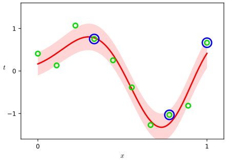
fig7_9. Download: PDF · SVG7.2.2 Analysis of sparsity
pp. 349–353 Why does maximising the evidence prune basis functions? First a geometric view, then an exact analysis that also yields a faster algorithm.
Result 7.16 (one basis function: when is it kept? The geometry of Figure 7.10) pp. 349–351, (7.92)
Take one basis vector \(\bm\varphi=(\phi(x_1),\dots,\phi(x_N))^\T\) and \(\mathbf{C}\)
Otherwise it increases as \(\alpha\to\infty\) and the basis vector is pruned. So a basis vector is pruned when it is poorly aligned with the data vector: \(t_\parallel^2=\|\mathbf{t}\|^2\cos^2\theta\) is small.
Proof
\(\mathbf{C}\) has eigenvalue \(v=\beta^{-1}+\|\bm\varphi\|^2/\alpha\) along \(\bm\varphi\) and \(\beta^{-1}\) in the \(N-1\) orthogonal directions. Hence \(\ln|\mathbf{C}|=(N-1)\ln\beta^{-1}+\ln v\) and \(\mathbf{t}^\T\mathbf{C}^{-1}\mathbf{t}\)
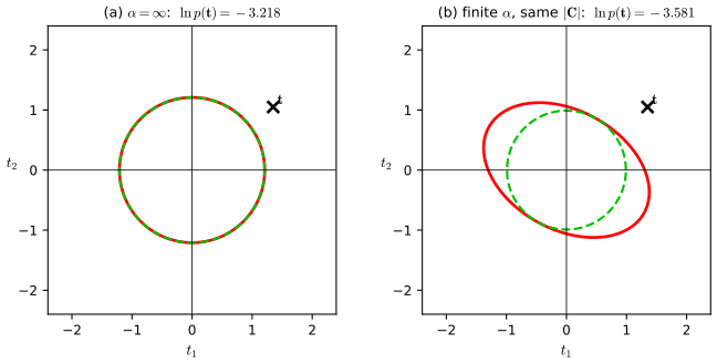
fig7_10. Download: PDF · SVGFor several basis vectors the same intuition holds. To make it exact, isolate the contribution of one hyperparameter. In (7.87) the right-hand side depends on \(\alpha_i\) itself (through \(m_i\) and \(\Sigma_{ii}\)), so it is only an implicit equation; instead we make the dependence on \(\alpha_i\) explicit (Faul and Tipping, 2002; Tipping and Faul, 2003). Write \(\bm\varphi_i\) for the \(i\)th column of \(\bm\Phi\) (the \(N\)-vector \((\phi_i(\mathbf{x}_1),\dots,\phi_i(\mathbf{x}_N))^\T\)), as opposed to \(\bm\phi_n\), the \(n\)th row.
Result 7.17 (the marginal likelihood as a function of one \(\alpha_i\); Exercise 7.15) pp. 351–352, (7.93)–(7.99)
Let \(\mathbf{C}_{-i}\)
Then
\[ |\mathbf{C}|=|\mathbf{C}_{-i}|\big(1+\alpha_i^{-1}\bm\varphi_i^\T\mathbf{C}_{-i}^{-1}\bm\varphi_i\big),\tag{7.94} \] \[ \mathbf{C}^{-1}=\mathbf{C}_{-i}^{-1}-\frac{\mathbf{C}_{-i}^{-1}\bm\varphi_i\bm\varphi_i^\T\mathbf{C}_{-i}^{-1}}{\alpha_i+\bm\varphi_i^\T\mathbf{C}_{-i}^{-1}\bm\varphi_i},\tag{7.95} \]and the log marginal likelihood splits as
\[ \mathcal{L}(\bm\alpha)=\mathcal{L}(\bm\alpha_{-i})+\lambda(\alpha_i),\tag{7.96} \] \[ \lambda(\alpha_i)=\frac12\Big[\ln\alpha_i-\ln(\alpha_i+s_i)+\frac{q_i^2}{\alpha_i+s_i}\Big],\tag{7.97} \]with the sparsity and quality factors
\[ s_i=\bm\varphi_i^\T\mathbf{C}_{-i}^{-1}\bm\varphi_i,\tag{7.98} \] \[ q_i=\bm\varphi_i^\T\mathbf{C}_{-i}^{-1}\mathbf{t}.\tag{7.99} \]Here \(\mathcal{L}(\bm\alpha_{-i})\) is the log marginal likelihood with \(\bm\varphi_i\) omitted.
Erratum. The book writes the right side of (7.94) with absolute-value bars around the bracket; the bracket is positive, so they are not needed (and the errata list corrects them to ordinary brackets).
Proof
(7.93): in (7.86), \(\bm\Phi\mathbf{A}^{-1}\bm\Phi^\T\)
Now take logarithms. From (7.94), with \(1+s_i/\alpha_i=(\alpha_i+s_i)/\alpha_i\),
\[ \ln|\mathbf{C}|=\ln|\mathbf{C}_{-i}|+\ln(\alpha_i+s_i)-\ln\alpha_i. \]From (7.95), \(\mathbf{t}^\T\mathbf{C}^{-1}\mathbf{t}\)
Interpretation: \(s_i\) measures how much \(\bm\varphi_i\) overlaps with the basis vectors already in the model (in the metric \(\mathbf{C}_{-i}^{-1}\)); \(q_i\) measures how well \(\bm\varphi_i\) is aligned with the error between \(\mathbf{t}\) and the prediction \(\mathbf{y}_{-i}\) of the model without \(\bm\varphi_i\).
Result 7.18 (stationary points and the pruning rule; Exercise 7.16) p. 352, (7.100)–(7.101)
The derivative of \(\lambda\) is
\[ \frac{\d\lambda(\alpha_i)}{\d\alpha_i}=\frac{\alpha_i^{-1}s_i^2-(q_i^2-s_i)}{2(\alpha_i+s_i)^2}.\tag{7.100} \](a) If \(q_i^2\gt s_i\), \(\lambda\) has a unique stationary point on \(\alpha_i\gt0\), which is its global maximum,
\[ \alpha_i=\frac{s_i^2}{q_i^2-s_i}.\tag{7.101} \](b) If \(q_i^2\le s_i\), \(\lambda\) is strictly increasing in \(\alpha_i\), so its supremum is at \(\alpha_i=\infty\): the basis function is pruned. (c) In case (a), including the basis function raises the log evidence over excluding it by \(\lambda(\alpha_i^\star)-\lambda(\infty)\)
Proof
(7.100). \(\lambda'\)
Signs. The denominator is positive, so the sign of \(\lambda'\) is that of \(h(\alpha)=s^2/\alpha-(q^2-s)\), a strictly decreasing function of \(\alpha\gt0\) going from \(+\infty\) at \(0^+\) to \(-(q^2-s)\) at \(\infty\). (a) If \(q^2\gt s\), \(h\) changes sign exactly once, at \(s^2/\alpha=q^2-s\), i.e. (7.101). \(\lambda'\gt0\) before and \(\lt0\) after, so this is the global maximum. (This is the "second derivative" check of Exercise 7.16: at the zero of \(h\), \(\lambda''\)
(c) At (7.101), \(\alpha+s=sq^2/(q^2-s)\), so \(\alpha/(\alpha+s)=s/q^2\) and \(q^2/(\alpha+s)=(q^2-s)/s\). Therefore \(\lambda(\alpha^\star)\)
Compare with Result 7.16: for one basis vector, \(\mathbf{C}_{-i}=\beta^{-1}\mathbf{I}\), so \(s=\beta\|\bm\varphi\|^2\), \(q=\beta\bm\varphi^\T\mathbf{t}\), and the condition \(q^2\gt s\) is \(\beta(\bm\varphi^\T\mathbf{t})^2\)
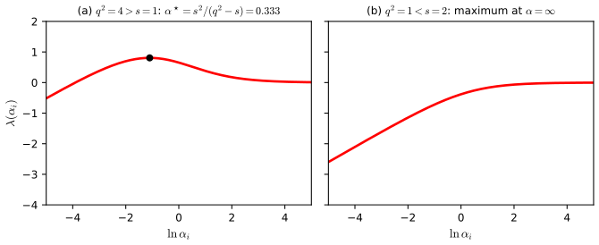
fig7_11. Download: PDF · SVGAlgorithm 7.2 (sequential sparse Bayesian learning) pp. 352–353
- (Regression) initialise \(\beta\).
- Start with one basis function \(\bm\varphi_1\), with \(\alpha_1\) from (7.101); set all other \(\alpha_j=\infty\) (excluded).
- Compute \(\bm\Sigma\) and \(\mathbf{m}\) (over the included basis functions) and \(q_i,s_i\) for all \(i\).
- Pick a candidate \(\bm\varphi_i\).
- If \(q_i^2\gt s_i\) and \(\alpha_i\lt\infty\) (already in): re-estimate \(\alpha_i\) by (7.101).
- If \(q_i^2\gt s_i\) and \(\alpha_i=\infty\): add \(\bm\varphi_i\) to the model with \(\alpha_i\) from (7.101).
- If \(q_i^2\le s_i\) and \(\alpha_i\lt\infty\): remove \(\bm\varphi_i\), set \(\alpha_i=\infty\). (If already excluded, do nothing.)
- (Regression) update \(\beta\).
- Stop when converged, else go to 3.
Each of steps 5 to 7 is an exact maximisation over one \(\alpha_i\) with the others fixed, so the log evidence never decreases (it increases by \(\lambda(\alpha^{\rm new})\)
Result 7.19 (computing \(s_i,q_i\) cheaply; Exercise 7.17) pp. 353, (7.102)–(7.107)
With the full \(\mathbf{C}\) (all included basis functions, whether or not \(\bm\varphi_i\) is among them) define
\[ Q_i=\bm\varphi_i^\T\mathbf{C}^{-1}\mathbf{t},\tag{7.102} \] \[ S_i=\bm\varphi_i^\T\mathbf{C}^{-1}\bm\varphi_i.\tag{7.103} \]Then
\[ q_i=\frac{\alpha_iQ_i}{\alpha_i-S_i},\tag{7.104} \] \[ s_i=\frac{\alpha_iS_i}{\alpha_i-S_i},\tag{7.105} \]so \(q_i=Q_i\), \(s_i=S_i\) when \(\alpha_i=\infty\), and in terms of the posterior quantities
\[ Q_i=\beta\bm\varphi_i^\T\mathbf{t}-\beta^2\bm\varphi_i^\T\bm\Phi\bm\Sigma\bm\Phi^\T\mathbf{t},\tag{7.106} \] \[ S_i=\beta\bm\varphi_i^\T\bm\varphi_i-\beta^2\bm\varphi_i^\T\bm\Phi\bm\Sigma\bm\Phi^\T\bm\varphi_i,\tag{7.107} \]where \(\bm\Phi,\bm\Sigma\) involve only basis vectors with finite \(\alpha\).
Proof
(7.106), (7.107). By the Woodbury identity applied to (7.86), \(\mathbf{C}^{-1}\)
(7.104), (7.105). Multiply (7.95) by \(\bm\varphi_i^\T\) on the left and \(\mathbf{t}\) (or \(\bm\varphi_i\)) on the right. Using the definitions (7.98), (7.99):
\[ Q_i=q_i-\frac{s_iq_i}{\alpha_i+s_i}=\frac{\alpha_iq_i}{\alpha_i+s_i},\qquad S_i=s_i-\frac{s_i^2}{\alpha_i+s_i}=\frac{\alpha_is_i}{\alpha_i+s_i}. \]Solve for \(s_i\): \(S_i(\alpha_i+s_i)\)
Filling the gap 7.7: updating \(\bm\Sigma\) and \(\mathbf{m}\) after changing one \(\alpha_i\) p. 353
The book says the required computations scale as \(O(M^3)\). In fact each step can be a rank-one update, \(O(M^2)\).
Derivation
If an included weight's precision changes from \(\alpha_i\) to \(\alpha_i^{\rm new}\), then \(\bm\Sigma^{-1}\) changes by \(\Delta\,\mathbf{e}_i\mathbf{e}_i^\T\) with \(\Delta=\alpha_i^{\rm new}-\alpha_i\) (only \(\mathbf{A}\) changes). Sherman-Morrison gives
\[ \bm\Sigma^{\rm new}=\bm\Sigma-\frac{\Delta\,\bm\Sigma\mathbf{e}_i\mathbf{e}_i^\T\bm\Sigma}{1+\Delta\Sigma_{ii}}=\bm\Sigma-\frac{\bm\Sigma_{:i}\bm\Sigma_{i:}}{\Delta^{-1}+\Sigma_{ii}}, \]and, since \(\mathbf{m}^{\rm new}\)
7.2.3 RVM for classification
pp. 353–356 For two classes with \(t\in\{0,1\}\) (the book's convention for the RVM) the model is logistic regression with the ARD prior (7.80):
\[ y(\mathbf{x},\mathbf{w})=\sigma\big(\mathbf{w}^\T\bm\phi(\mathbf{x})\big).\tag{7.108} \]The integral over \(\mathbf{w}\) is no longer analytic, so use the Laplace approximation (Section 4.4) at the current \(\bm\alpha\), maximise the resulting approximate marginal likelihood over \(\bm\alpha\), and repeat. The log posterior of \(\mathbf{w}\) is
\[ \ln p(\mathbf{w}\given\mathbf{t},\bm\alpha)=\ln\{p(\mathbf{t}\given\mathbf{w})p(\mathbf{w}\given\bm\alpha)\}-\ln p(\mathbf{t}\given\bm\alpha)=\sum_{n=1}^{N}\{t_n\ln y_n+(1-t_n)\ln(1-y_n)\}-\frac12\mathbf{w}^\T\mathbf{A}\mathbf{w}+\const.\tag{7.109} \]Result 7.20 (gradient, Hessian and the Laplace approximation; Exercise 7.18) pp. 354, (7.110)–(7.113)
With \(\mathbf{y}=(y_1,\dots,y_N)^\T\) and \(\mathbf{B}=\diag(b_n)\), \(b_n=y_n(1-y_n)\),
\[ \nabla\ln p(\mathbf{w}\given\mathbf{t},\bm\alpha)=\bm\Phi^\T(\mathbf{t}-\mathbf{y})-\mathbf{A}\mathbf{w},\tag{7.110} \] \[ \nabla\nabla\ln p(\mathbf{w}\given\mathbf{t},\bm\alpha)=-\big(\bm\Phi^\T\mathbf{B}\bm\Phi+\mathbf{A}\big).\tag{7.111} \]The Hessian is negative definite, so the log posterior is concave (IRLS, Section 4.3.3, converges to the unique mode). At the mode,
\[ \mathbf{w}^\star=\mathbf{A}^{-1}\bm\Phi^\T(\mathbf{t}-\mathbf{y}),\tag{7.112} \] \[ \bm\Sigma=\big(\bm\Phi^\T\mathbf{B}\bm\Phi+\mathbf{A}\big)^{-1},\tag{7.113} \]and the posterior is approximated by \(\N(\mathbf{w}\given\mathbf{w}^\star,\bm\Sigma)\). (Note that (7.112) is an implicit equation: \(\mathbf{y}\) depends on \(\mathbf{w}^\star\).)
Proof
With \(a_n=\mathbf{w}^\T\bm\phi_n\) and \(y_n=\sigma(a_n)\), \(\sigma'(a)=\sigma(1-\sigma)\) (4.88). The data term has \(\frac{\partial}{\partial a_n}\{t_n\ln y_n\)
The Laplace approximation (4.135) of the marginal likelihood is
\[ p(\mathbf{t}\given\bm\alpha)=\int p(\mathbf{t}\given\mathbf{w})p(\mathbf{w}\given\bm\alpha)\,\d\mathbf{w}\simeq p(\mathbf{t}\given\mathbf{w}^\star)\,p(\mathbf{w}^\star\given\bm\alpha)\,(2\pi)^{M/2}|\bm\Sigma|^{1/2}.\tag{7.114} \]Result 7.21 (hyperparameter updates and the equivalent regression problem; Exercise 7.19) pp. 355, (7.115)–(7.119)
Maximising (7.114) over \(\alpha_i\) (holding \(\mathbf{B}\) fixed) gives
\[ -\frac12(w_i^\star)^2+\frac1{2\alpha_i}-\frac12\Sigma_{ii}=0,\tag{7.115} \] \[ \alpha_i^{\rm new}=\frac{\gamma_i}{(w_i^\star)^2},\qquad\gamma_i=1-\alpha_i\Sigma_{ii},\tag{7.116} \]the same formula as (7.87). Define the effective targets and the matrix
\[ \hat{\mathbf{t}}=\bm\Phi\mathbf{w}^\star+\mathbf{B}^{-1}(\mathbf{t}-\mathbf{y}),\tag{7.117} \] \[ \mathbf{C}=\mathbf{B}^{-1}+\bm\Phi\mathbf{A}^{-1}\bm\Phi^\T.\tag{7.119} \]Then, as a function of \(\bm\alpha\) (with \(\mathbf{B}\) and \(\hat{\mathbf{t}}\) held fixed), the approximate log marginal likelihood has the same gradient as
\[ \ln p(\mathbf{t}\given\bm\alpha)=-\frac12\Big\{N\ln(2\pi)+\ln|\mathbf{C}|+\hat{\mathbf{t}}^\T\mathbf{C}^{-1}\hat{\mathbf{t}}\Big\},\tag{7.118} \]so the sparsity analysis of Section 7.2.2 and the fast sequential algorithm apply unchanged, with \(\hat{\mathbf{t}}\) as the targets and \(\mathbf{B}^{-1}\) as the noise covariance.
Errata. The book prints \(\ln p(\mathbf{t}\given\bm\alpha,\beta)\) in (7.118); there is no \(\beta\) in the classification model, so it is \(\ln p(\mathbf{t}\given\bm\alpha)\). The exercise statement 7.19 should say "approximate marginal" and not "approximate log marginal". The book prints (7.119) as \(\mathbf{C}\)
Derivation
(7.115). Take the log of (7.114): \(\ln p(\mathbf{t}\given\bm\alpha)\)
(7.116). Multiply (7.115) by \(2\alpha_i\): \(-\alpha_i(w_i^\star)^2+1-\alpha_i\Sigma_{ii}=0\), i.e. \(\alpha_i(w_i^\star)^2=\gamma_i\).
(7.117)–(7.119). Consider the Gaussian regression problem \(\hat{\mathbf{t}}\)
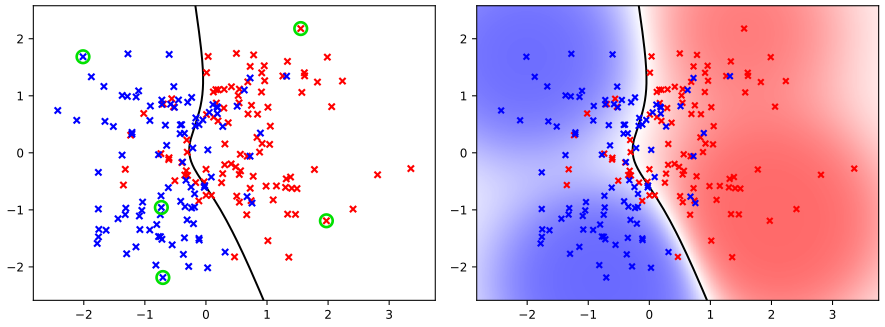
fig7_12. Download: PDF · SVGWhy do the relevance vectors avoid the boundary? A basis function centred on a point near the decision boundary has a vector \(\bm\varphi_i\) that is poorly aligned with the target vector (the kernel is large for points of both classes), so \(q_i^2\) is small compared with \(s_i\) and it is pruned (Result 7.18). An SVM, in contrast, keeps exactly the points at the boundary.
More than two classes. Use \(K\) linear models \(a_k=\mathbf{w}_k^\T\mathbf{x}\) (7.120), a softmax (7.121), \(y_k=\exp(a_k)/\sum_j\exp(a_j)\), and the log likelihood with 1-of-\(K\) targets \(t_{nk}\),
\[ \ln p(\mathbf{T}\given\mathbf{w}_1,\dots,\mathbf{w}_K)=\sum_{n=1}^{N}\sum_{k=1}^{K}t_{nk}\ln y_{nk}\tag{7.122} \](The book prints the product, i.e. \(p\) and not \(\ln p\); the logarithm is the sum.) The Laplace approximation and hyperparameter optimisation proceed as before using IRLS (Tipping, 2001). This is a more principled multiclass method than the pairwise SVM schemes and gives probabilities, but the Hessian is \(MK\times MK\), so training is a factor \(K^3\) more costly than the two-class RVM.
The RVM and the SVM compared
| Support vector machine | Relevance vector machine | |
|---|---|---|
| Output | decision only (Platt scaling for probabilities) | full predictive distribution, mean and variance |
| Training problem | convex QP, global optimum | maximisation of a non-convex evidence; local maxima possible |
| Complexity parameters | \(C\), \(\epsilon\) or \(\nu\), kernel parameters by cross-validation (several runs) | \(\bm\alpha,\beta\) by evidence maximisation in one run (kernel parameters still need a choice) |
| Kernel | positive definite, centred on data | any basis functions, not tied to the data |
| Sparsity | support vectors: on or inside the margin or tube; grows with the data | relevance vectors: typically an order of magnitude fewer, away from the boundary |
| Multiclass | combinations of two-class machines | softmax model, cost factor \(K^3\) |
| Training time | about \(O(N^2)\) (SMO) | \(O(M^3)\), longer; faster with Algorithm 7.2 |
| Test time | number of support vectors | number of relevance vectors, typically much smaller |
| Behaviour far from data | decision from the sign of \(y\) | RVM variance collapses to noise (over-confident) |
Exercises
All 19 exercises of Chapter 7 (Bishop, 2006, pp. 357–358), restated in my own words, with complete solutions (hidden). Stars give the book's difficulty and "www" marks the exercises with official solutions. Most exercises are derivations used above; their solutions give the argument and link to the full version where it already appears. Solution manuals contain slips: the closest-mean remark in Exercise 7.1 is one.
Exercise 7.1 (★★, www). Model the inputs of each class (labels \(t_n\in\{-1,1\}\)) with a Parzen density estimator with kernel \(k(\mathbf{x},\mathbf{x}')\). Write the minimum misclassification-rate rule for equal priors. Show that for \(k(\mathbf{x},\mathbf{x}')\)
\({}=\mathbf{x}^\T\mathbf{x}'\) it reduces to comparing inner products with the class means, and that for \(k=\bm\phi(\mathbf{x})^\T\bm\phi(\mathbf{x}')\) the same holds in feature space. Solution
Let \(N_\pm\) be the class sizes. The Parzen estimates are \(p(\mathbf{x}\given t=\pm1)\)
\[ \hat t(\mathbf{x})=\operatorname{sign}\Big(\frac1{N_+}\sum_{n:t_n=+1}k(\mathbf{x},\mathbf{x}_n)-\frac1{N_-}\sum_{n:t_n=-1}k(\mathbf{x},\mathbf{x}_n)\Big)=\operatorname{sign}\Big(\sum_n\frac{t_n}{N_{t_n}}k(\mathbf{x},\mathbf{x}_n)\Big). \]\({}=\frac1{N_\pm}\sum_{n:t_n=\pm1}\frac1{Z_k}k(\mathbf{x},\mathbf{x}_n)\), with \(Z_k\) the normalising constant of the kernel (the same for both classes). With equal priors, \(p(t\given\mathbf{x})\) \({}\propto p(\mathbf{x}\given t)\), and the misclassification rate is minimised by choosing the class with the larger posterior, so For \(k(\mathbf{x},\mathbf{x}')\)
\({}=\mathbf{x}^\T\mathbf{x}'\) (improper as a density, but the comparison is still meaningful), \(\frac1{N_\pm}\sum_{\pm}\mathbf{x}^\T\mathbf{x}_n\) \({}=\mathbf{x}^\T\bar{\mathbf{x}}_\pm\) with the class mean \(\bar{\mathbf{x}}_\pm\), so \(\hat t\) \({}=\operatorname{sign}\{\mathbf{x}^\T(\bar{\mathbf{x}}_+-\bar{\mathbf{x}}_-)\}\): assign to the class whose mean has the larger inner product with \(\mathbf{x}\). The same algebra with \(k=\bm\phi^\T\bm\phi\) gives \(\hat t\) \({}=\operatorname{sign}\{\bm\phi(\mathbf{x})^\T(\bar{\bm\phi}_+-\bar{\bm\phi}_-)\}\), with the means of the feature vectors. Caveat. This is "closest mean" in the sense of the larger inner product. Exactly closest in Euclidean distance would be \(\|\mathbf{x}-\bar{\mathbf{x}}_+\|^2\)
\({}\lt\|\mathbf{x}-\bar{\mathbf{x}}_-\|^2\) \({}\iff\mathbf{x}^\T(\bar{\mathbf{x}}_+-\bar{\mathbf{x}}_-)\) \({}\gt\frac12(\|\bar{\mathbf{x}}_+\|^2-\|\bar{\mathbf{x}}_-\|^2)\), which differs by a threshold unless the two mean vectors have equal norm. Using a normalised kernel such as the Gaussian removes the issue in the Parzen setting. Exercise 7.2 (★). Show that replacing the 1 in the constraint (7.5) by any \(\gamma\gt0\) leaves the maximum margin hyperplane unchanged.
Solution
Result 7.1(c): feasible set of the \(\gamma\)-problem is \(\gamma\) times that of (7.5), the objective scales by \(\gamma^2\), so the minimiser is \(\gamma(\mathbf{w},b)\), the same hyperplane \(\{y=0\}\) with margin \(\gamma/\|\gamma\mathbf{w}\|=1/\|\mathbf{w}\|\) unchanged. (This is the same as the freedom \(\kappa\) in (7.4).)
Exercise 7.3 (★★). Show that, whatever the dimension of the data space, a data set of just two points, one from each class, determines the maximum margin hyperplane.
Solution
Let the feature vectors be \(\bm\phi_+\ne\bm\phi_-\), \(d=\|\bm\phi_+-\bm\phi_-\|\). The balance constraint (7.12) is \(a_+-a_-=0\), so \(a_+=a_-=a\ge0\). Since \(t_+t_-=-1\), the dual (7.10) is
\[ \widetilde L(a)=2a-\tfrac12a^2(k_{++}+k_{--}-2k_{+-})=2a-\tfrac12a^2d^2, \]maximised at \(a=2/d^2\gt0\). By (7.8), \(\mathbf{w}\)
\({}=a(\bm\phi_+-\bm\phi_-)\) \({}=2(\bm\phi_+-\bm\phi_-)/d^2\), so \(\|\mathbf{w}\|=2/d\), the margin is \(\rho=d/2\), and both points are support vectors. The bias comes from \(t_+y_+=1\): \(b=1-\mathbf{w}^\T\bm\phi_+\). The midpoint \(\bar{\bm\phi}=(\bm\phi_++\bm\phi_-)/2\) has \(y(\bar{\bm\phi})\) \({}=\mathbf{w}^\T\bar{\bm\phi}+1\) \({}-\mathbf{w}^\T\bm\phi_+\) \({}=\mathbf{w}^\T(\bm\phi_--\bm\phi_+)/2+1\) \({}=-\frac{2}{d^2}\cdot\frac{d^2}2+1\) \({}=0\). Hence the hyperplane is the perpendicular bisector of the segment joining the two points (its normal \(\mathbf{w}\) is parallel to \(\bm\phi_+-\bm\phi_-\)). Geometrically: any separating hyperplane has distances \(r_+\) and \(r_-\) to the two points on opposite sides with \(r_++r_-\le d\) (the segment crosses it), so the margin is at most \(d/2\), with equality only for the bisector. Only \(d\) enters, so the dimension of the space plays no role. (In input space with a nonlinear kernel, this bisector is a curved surface.) Exercise 7.4 (★★, www). Show that the margin \(\rho\) of the maximum margin hyperplane satisfies \(\rho^{-2}=\sum_na_n\), with \(\{a_n\}\) maximising (7.10) under (7.11), (7.12).
Solution
See Result 7.5. In short: \(\rho=1/\|\mathbf{w}\|\); by (7.8), (7.9) and \(\bm\phi_n^\T\mathbf{w}=y_n-b\), \(\|\mathbf{w}\|^2=\sum_na_nt_ny_n\); by (7.16) \(a_nt_ny_n=a_n\); so \(\rho^{-2}=\|\mathbf{w}\|^2=\sum_na_n\).
Exercise 7.5 (★★). Show that also \(\rho^{-2}=2\widetilde L(\mathbf{a})\) and \(\rho^{-2}=\|\mathbf{w}\|^2\).
Solution
See Result 7.5. The second is the definition of the margin in canonical form, (7.4). For the first, (7.8) turns the quadratic term of (7.10) into \(\frac12\|\mathbf{w}\|^2\), so \(\widetilde L=\sum_na_n-\frac12\|\mathbf{w}\|^2\), and with \(\sum_na_n=\|\mathbf{w}\|^2\) from Exercise 7.4, \(\widetilde L\)
\({}=\frac12\|\mathbf{w}\|^2\) \({}=\frac1{2\rho^2}\). (Consistency: at the optimum the primal value \(\frac12\|\mathbf{w}\|^2\) equals the dual value, as strong duality says.) Exercise 7.6 (★). For logistic regression with \(t\in\{-1,1\}\), \(p(t=1\given y)=\sigma(y)\), show that the regularised negative log likelihood is (7.47).
Solution
See Result 7.8. \(p(t=-1\given y)=1-\sigma(y)=\sigma(-y)\), so \(p(t\given y)=\sigma(yt)\) for both values of \(t\). The negative log of the product over independent observations is \(-\sum_n\ln\sigma(y_nt_n)\)
\({}=\sum_n\ln(1+e^{-y_nt_n})\), and adding the regulariser \(\lambda\|\mathbf{w}\|^2\) (the negative log of a Gaussian prior up to constants) gives (7.47), (7.48). Exercise 7.7 (★). From the Lagrangian (7.56) of SVM regression, set the derivatives with respect to \(\mathbf{w},b,\xi_n,\hat\xi_n\) to zero and back-substitute to obtain the dual (7.61).
Solution
Done in full in Result 7.9: the stationarity conditions are (7.57)–(7.60); the slack terms cancel because of (7.59), (7.60); the remaining terms are \(\frac12\|\mathbf{w}\|^2\)
\({}-\epsilon\sum(a_n+\hat a_n)\) \({}+\sum(a_n-\hat a_n)t_n-\sum(a_n-\hat a_n)y_n\), and \(\sum(a_n-\hat a_n)y_n=\|\mathbf{w}\|^2\) by (7.57), (7.58), which leaves (7.61). Exercise 7.8 (★, www). In SVM regression, show that every point with \(\xi_n\gt0\) has \(a_n=C\), and every point with \(\hat\xi_n\gt0\) has \(\hat a_n=C\).
Solution
The KKT conditions for the constraints \(\xi_n\ge0\) are \(\mu_n\ge0\) and \(\mu_n\xi_n=0\). If \(\xi_n\gt0\), then \(\mu_n=0\); stationarity in \(\xi_n\), (7.59), gives \(a_n=C-\mu_n=C\). The same with hats and (7.60) gives \(\hat a_n=C\). Equivalently (7.67), (7.68).
Exercise 7.9 (★). Verify the posterior mean and covariance (7.82), (7.83) of the regression RVM.
Solution
Result 7.12: the log posterior is \(-\frac12\mathbf{w}^\T(\mathbf{A}+\beta\bm\Phi^\T\bm\Phi)\mathbf{w}\)
\({}+\beta\mathbf{w}^\T\bm\Phi^\T\mathbf{t}+\const\); matching to \(-\frac12(\mathbf{w}-\mathbf{m})^\T\bm\Sigma^{-1}(\mathbf{w}-\mathbf{m})\) gives \(\bm\Sigma^{-1}=\mathbf{A}+\beta\bm\Phi^\T\bm\Phi\) and \(\bm\Sigma^{-1}\mathbf{m}\) \({}=\beta\bm\Phi^\T\mathbf{t}\). Exercise 7.10 (★★, www). Derive the marginal likelihood (7.85) by performing the Gaussian integral over \(\mathbf{w}\) in (7.84) with completing the square.
Solution
Route 2 of Result 7.13: the integrand is a constant times \(\exp\{-\frac12(\mathbf{w}-\mathbf{m})^\T\bm\Sigma^{-1}(\mathbf{w}-\mathbf{m})\)
\({}-E(\mathbf{m})\}\); integrating gives \((2\pi)^{M/2}|\bm\Sigma|^{1/2}\) and the form \((*)\), which equals (7.85) by the determinant lemma and the Woodbury identity (shown there). Exercise 7.11 (★★). Repeat Exercise 7.10 using the general result (2.115).
Solution
Route 1 of Result 7.13. With prior \(\mathbf{w}\)
\({}\sim\N(\bm\mu=\mathbf{0},\bm\Lambda^{-1}=\mathbf{A}^{-1})\) and conditional \(\mathbf{t}\given\mathbf{w}\) \({}\sim\N(\bm\Phi\mathbf{w},\mathbf{L}^{-1}=\beta^{-1}\mathbf{I})\), (2.115) says \(p(\mathbf{t})\) \({}=\N(\bm\Phi\bm\mu,\mathbf{L}^{-1}+\bm\Phi\bm\Lambda^{-1}\bm\Phi^\T)\) \({}=\N(\mathbf{0},\beta^{-1}\mathbf{I}+\bm\Phi\mathbf{A}^{-1}\bm\Phi^\T)\) \({}=\N(\mathbf{0},\mathbf{C})\). Exercise 7.12 (★★, www). Show that direct maximisation of (7.85) gives the re-estimation equations (7.87), (7.88) with \(\gamma_i\) as in (7.89).
Solution
Result 7.14: differentiate \((*)\); the dependence through \(\mathbf{m}\) vanishes because \(\mathbf{m}\) minimises \(E\). The derivative in \(\alpha_i\) is \(\frac1{2\alpha_i}-\frac12\Sigma_{ii}\)
\({}-\frac12m_i^2\); in \(\beta\), \(\frac N{2\beta}-\frac12\|\mathbf{t}\) \({}-\bm\Phi\mathbf{m}\|^2\) \({}-\frac1{2\beta}\sum_i\gamma_i\), using \(\beta\Tr(\bm\Sigma\bm\Phi^\T\bm\Phi)\) \({}=\sum_i\gamma_i\). Exercise 7.13 (★★). Add Gamma hyperpriors \(p(\alpha_i)=\Gam(\alpha_i\given a,b)\), \(p(\beta)=\Gam(\beta\given c,d)\) and obtain the re-estimation formulae by maximising the posterior \(p(\mathbf{t},\bm\alpha,\beta\given\mathbf{X})\).
Solution
With \(\Gam(\lambda\given a,b)\)
\({}\propto\lambda^{a-1}e^{-b\lambda}\) (toolkit), the objective is \(\ln p(\mathbf{t}\given\bm\alpha,\beta)\) \({}+\sum_i\{(a-1)\ln\alpha_i-b\alpha_i\}\) \({}+(c-1)\ln\beta-d\beta+\const\). The extra derivatives are \((a-1)/\alpha_i-b\) and \((c-1)/\beta-d\). Add them to the derivatives of Result 7.14. For \(\alpha_i\): \(\frac1{2\alpha_i}-\frac12\Sigma_{ii}\)
\[ \alpha_i^{\rm new}=\frac{\gamma_i+2a-2}{m_i^2+2b}. \]\({}-\frac12m_i^2+\frac{a-1}{\alpha_i}-b\) \({}=0\). Multiply by \(2\alpha_i\): \(1-\alpha_i\Sigma_{ii}-\alpha_im_i^2+2(a-1)\) \({}-2b\alpha_i\) \({}=0\), i.e. \(\alpha_i(m_i^2+2b)=\gamma_i+2a-2\): For \(\beta\): \(\frac N{2\beta}-\frac12\|\mathbf{t}\)
\[ \beta^{\rm new}=\frac{N-\sum_i\gamma_i+2c-2}{\|\mathbf{t}-\bm\Phi\mathbf{m}\|^2+2d}. \]\({}-\bm\Phi\mathbf{m}\|^2\) \({}-\frac{\sum_i\gamma_i}{2\beta}+\frac{c-1}\beta\) \({}-d\) \({}=0\). Multiply by \(2\beta\): \(N-\sum_i\gamma_i-\beta\|\mathbf{t}\) \({}-\bm\Phi\mathbf{m}\|^2+2(c-1)-2d\beta\) \({}=0\): Checks: \(a=1,b=0,c=1,d=0\) (flat hyperpriors) recovers (7.87), (7.88). The Gamma shape \(a\lt1\) with small rate (a typical "non-informative" choice, \(a,b\to0\)) lowers the numerator by about 2 and makes pruning more aggressive (this is a statement about the mode of the density in \(\alpha\), which is not invariant under reparametrisation).
Exercise 7.14 (★★). Derive the predictive distribution (7.90) of the regression RVM and its variance (7.91).
Solution
Result 7.15: \(t=\mathbf{w}^\T\bm\phi+\varepsilon\), with \(\mathbf{w}\sim\N(\mathbf{m},\bm\Sigma)\) and independent noise \(\varepsilon\sim\N(0,(\beta^\star)^{-1})\); the sum is Gaussian with mean \(\mathbf{m}^\T\bm\phi\) and variance \((\beta^\star)^{-1}+\bm\phi^\T\bm\Sigma\bm\phi\) (the linear-Gaussian rule, (2.115)).
Exercise 7.15 (★★, www). Using (7.94), (7.95), show that (7.85) can be written as (7.96) with \(\lambda\) in (7.97), \(s_i\) and \(q_i\) in (7.98), (7.99).
Solution
Result 7.17: \(\ln|\mathbf{C}|\)
\({}=\ln|\mathbf{C}_{-i}|+\ln(\alpha_i+s_i)\) \({}-\ln\alpha_i\) and \(\mathbf{t}^\T\mathbf{C}^{-1}\mathbf{t}\) \({}=\mathbf{t}^\T\mathbf{C}_{-i}^{-1}\mathbf{t}\) \({}-q_i^2/(\alpha_i+s_i)\); insert in (7.85). Exercise 7.16 (★). Show by the second derivative that the stationary point (7.101) of the log marginal likelihood is a maximum.
Solution
Result 7.18. Write \(\lambda'=h(\alpha)/(2(\alpha+s)^2)\) with \(h=s^2/\alpha-(q^2-s)\). At a zero of \(h\), the second term of the product rule vanishes and \(\lambda''\)
\({}=h'(\alpha)/(2(\alpha+s)^2)\) \({}=-s^2/(2\alpha^2(\alpha+s)^2)\) \({}\lt0\). In fact \(h\) is strictly decreasing, which also proves uniqueness (and global maximality) of the stationary point when \(q^2\gt s\). Exercise 7.17 (★★). Using (7.83), (7.86) and the Woodbury identity (C.7), show that \(Q_i\) and \(S_i\) of (7.102), (7.103) take the form (7.106), (7.107).
Solution
Result 7.19: Woodbury applied to \(\mathbf{C}\)
\({}=\beta^{-1}\mathbf{I}\) \({}+\bm\Phi\mathbf{A}^{-1}\bm\Phi^\T\) gives \(\mathbf{C}^{-1}\) \({}=\beta\mathbf{I}\) \({}-\beta^2\bm\Phi(\mathbf{A}+\beta\bm\Phi^\T\bm\Phi)^{-1}\bm\Phi^\T\) \({}=\beta\mathbf{I}\) \({}-\beta^2\bm\Phi\bm\Sigma\bm\Phi^\T\). Then \(Q_i=\bm\varphi_i^\T\mathbf{C}^{-1}\mathbf{t}\) and \(S_i=\bm\varphi_i^\T\mathbf{C}^{-1}\bm\varphi_i\) give (7.106), (7.107). Exercise 7.18 (★, www). Show that the gradient and Hessian of the log posterior (7.109) of the classification RVM are (7.110), (7.111).
Solution
Result 7.20: \(\partial\ell_n/\partial a_n=t_n-y_n\) for \(\ell_n=t_n\ln y_n+(1-t_n)\ln(1-y_n)\) with \(y_n=\sigma(a_n)\) and \(\sigma'=\sigma(1-\sigma)\); \(\partial a_n/\partial\mathbf{w}=\bm\phi_n\); the prior contributes \(-\mathbf{A}\mathbf{w}\) and, on differentiating again, \(-\mathbf{A}\). The second derivative of the data term is \(-\sum_ny_n(1-y_n)\bm\phi_n\bm\phi_n^\T\)
\({}=-\bm\Phi^\T\mathbf{B}\bm\Phi\). Exercise 7.19 (★★). Show that maximising the approximate marginal likelihood (7.114) of the classification RVM gives the re-estimation (7.116).
Solution
Result 7.21. Differentiate \(\ln p(\mathbf{t}\given\mathbf{w}^\star)\)
\({}+\ln p(\mathbf{w}^\star\given\bm\alpha)\) \({}+\frac12\ln|\bm\Sigma|\) in \(\alpha_i\): the dependence through \(\mathbf{w}^\star\) vanishes (stationarity), the prior gives \(\frac1{2\alpha_i}-\frac12(w_i^\star)^2\), and \(\frac12\ln|\bm\Sigma|\) gives \(-\frac12\Sigma_{ii}\) when \(\mathbf{B}\) is held fixed, which is (7.115); then \(\alpha_i(w_i^\star)^2\) \({}=1-\alpha_i\Sigma_{ii}\) \({}=\gamma_i\). Note that holding \(\mathbf{B}\) fixed is an approximation (the book's), not an exact statement.
Demonstrations for this chapter
Each demonstration runs in the browser, with seeded random numbers so that a class sees the same pictures, and links back to these notes. The ▶ Demo boxes above open them already set to the case under discussion.
| Demonstration | What you can see | Sections and results |
|---|---|---|
| Support vector machines: margin, soft margin, kernels and regression | Maximum margin classifier, support vectors, the soft-margin constant \(C\), Gaussian kernels, and SVM regression with the ε-tube. Presets: 1 maximum margin, separable data (Figs 7.1, 7.2); 2 Gaussian kernel (Fig 7.2); 3 overlapping classes, soft margin (Fig 7.4); 4 the effect of \(C\); 5 SVM regression and its ε-tube (Fig 7.8); 6 only the support vectors matter. | 7.1, 7.1.1, 7.1.4; Results 7.2, 7.3, 7.6, 7.9 |
| Relevance vector machines compared with the SVM | RVM regression and classification, evidence maximisation of \(\bm\alpha\) and \(\beta\), and the comparison of relevance vectors with support vectors. Presets: 1 RVM regression, few relevance vectors (Fig 7.9); 2 hyperparameter evidence updates; 3 RVM classification (Fig 7.12); 4 RVM versus SVM sparsity (classification panels of Figs 7.4 and 7.12); 5 noise level and relevance vectors. | 7.2.1, 7.2.2, 7.2.3; Results 7.14, 7.18, 7.21 |
The Python code that produces every figure of this page, and checks the chapter's identities numerically, is code/ch07_sparse_kernel_machines.py (see the code index).
References
- Bishop, C. M. (2006). Pattern Recognition and Machine Learning. Springer, New York. Chapter 7, pp. 325–358.
- Allwein, E. L., Schapire, R. E. and Singer, Y. (2000). Reducing multiclass to binary: a unifying approach for margin classifiers. Journal of Machine Learning Research, 1, 113–141.
- Boser, B. E., Guyon, I. M. and Vapnik, V. N. (1992). A training algorithm for optimal margin classifiers. In Proceedings of the Fifth Annual Workshop on Computational Learning Theory, 144–152. doi:10.1145/130385.130401.
- Burges, C. J. C. (1998). A tutorial on support vector machines for pattern recognition. Data Mining and Knowledge Discovery, 2(2), 121–167. doi:10.1023/A:1009715923555.
- Cortes, C. and Vapnik, V. (1995). Support-vector networks. Machine Learning, 20(3), 273–297. doi:10.1007/BF00994018.
- Dietterich, T. G. and Bakiri, G. (1995). Solving multiclass learning problems via error-correcting output codes. Journal of Artificial Intelligence Research, 2, 263–286. doi:10.1613/jair.105.
- Faul, A. C. and Tipping, M. E. (2002). Analysis of sparse Bayesian learning. In Advances in Neural Information Processing Systems 14, 383–389. MIT Press.
- Lee, Y., Lin, Y. and Wahba, G. (2004). Multicategory support vector machines: theory and application to the classification of microarray data and satellite radiance data. Journal of the American Statistical Association, 99(465), 67–81. doi:10.1198/016214504000000098. (The book cites the 2001 technical report.)
- MacKay, D. J. C. (1992). Bayesian interpolation. Neural Computation, 4(3), 415–447. doi:10.1162/neco.1992.4.3.415. (The evidence approximation behind (7.87)–(7.88).)
- McAllester, D. A. (2003). PAC-Bayesian stochastic model selection. Machine Learning, 51(1), 5–21. doi:10.1023/A:1021840411064.
- Osuna, E., Freund, R. and Girosi, F. (1996). An improved training algorithm for support vector machines. In Neural Networks for Signal Processing VII, 276–285.
- Platt, J. C. (1999). Fast training of support vector machines using sequential minimal optimization. In Advances in Kernel Methods: Support Vector Learning, 185–208. MIT Press.
- Platt, J. C. (2000). Probabilistic outputs for support vector machines and comparisons to regularized likelihood methods. In Advances in Large Margin Classifiers, 61–73. MIT Press.
- Platt, J. C., Cristianini, N. and Shawe-Taylor, J. (2000). Large margin DAGs for multiclass classification. In Advances in Neural Information Processing Systems 12, 547–553. MIT Press.
- Rasmussen, C. E. and Quiñonero-Candela, J. (2005). Healing the relevance vector machine through augmentation. In Proceedings of the 22nd International Conference on Machine Learning, 689–696.
- Schölkopf, B., Smola, A. J., Williamson, R. C. and Bartlett, P. L. (2000). New support vector algorithms. Neural Computation, 12(5), 1207–1245. doi:10.1162/089976600300015565.
- Schölkopf, B., Platt, J. C., Shawe-Taylor, J., Smola, A. J. and Williamson, R. C. (2001). Estimating the support of a high-dimensional distribution. Neural Computation, 13(7), 1443–1471. doi:10.1162/089976601750264965.
- Smola, A. J. and Schölkopf, B. (2004). A tutorial on support vector regression. Statistics and Computing, 14(3), 199–222. doi:10.1023/B:STCO.0000035301.49549.88.
- Tax, D. M. J. and Duin, R. P. W. (1999). Support vector domain description. Pattern Recognition Letters, 20(11–13), 1191–1199. doi:10.1016/S0167-8655(99)00087-2.
- Tipping, M. E. (2001). Sparse Bayesian learning and the relevance vector machine. Journal of Machine Learning Research, 1, 211–244.
- Tipping, M. E. and Faul, A. C. (2003). Fast marginal likelihood maximisation for sparse Bayesian models. In Proceedings of the Ninth International Workshop on Artificial Intelligence and Statistics.
- Tong, S. and Koller, D. (2000). Restricted Bayes optimal classifiers. In Proceedings of the 17th National Conference on Artificial Intelligence, 658–664.
- Valiant, L. G. (1984). A theory of the learnable. Communications of the ACM, 27(11), 1134–1142. doi:10.1145/1968.1972.
- Vapnik, V. N. (1995). The Nature of Statistical Learning Theory. Springer, New York. (2nd edition 2000.)
- Vapnik, V. N. (1998). Statistical Learning Theory. Wiley, New York.
- Vapnik, V. N. and Chervonenkis, A. Ya. (1971). On the uniform convergence of relative frequencies of events to their probabilities. Theory of Probability and its Applications, 16(2), 264–280. doi:10.1137/1116025.
- Veropoulos, K., Campbell, C. and Cristianini, N. (1999). Controlling the sensitivity of support vector machines. In Proceedings of the International Joint Conference on Artificial Intelligence, 55–60.
- Weston, J. and Watkins, C. (1999). Support vector machines for multi-class pattern recognition. In Proceedings of the Seventh European Symposium on Artificial Neural Networks, 219–224.
DOIs were checked against Crossref; references without a DOI have none that I could verify. The numerical statements made in the text (the RVM marginal likelihood in its two forms, the stationarity conditions for \(\alpha_i\) and \(\beta\), the sparsity decomposition (7.96)–(7.99), the formulas (7.104)–(7.107) and the Laplace-approximation equivalence) were checked on random examples with numpy.