Linear Discriminant Analysis
A generative classifier models how the features are produced inside each class and then inverts the model with Bayes' rule. With Gaussian class-conditional densities this gives quadratic decision boundaries, and with one covariance shared by all classes the boundaries become linear: linear discriminant analysis. The chapter fits these models by maximum likelihood, regularises their covariances, relates them to logistic regression and to the nearest-centroid rule, derives Fisher's directions of best class separation, and then drops the Gaussian assumption for the independence assumption of naive Bayes. It closes with the trade-offs between generative and discriminative classifiers. The notes prove everything the book states without argument and add the numerical evidence for the claims it leaves open.
Ch. 1 Introduction Ch. 2 Univariate probability Ch. 3 Multivariate probability Ch. 4 Statistics Ch. 5 Decision theory Ch. 6 Information theory Ch. 7 Linear algebra Ch. 8 Optimisation Ch. 9 Discriminant analysis Ch. 10 Logistic regression Ch. 11 Linear regression Ch. 12 GLMs Ch. 13 Networks for tabular data Ch. 14 Networks for images Ch. 15 Networks for sequences Ch. 16 Exemplar-based methods Ch. 17 Kernel methods Ch. 18 Trees and boosting Ch. 19 Fewer labels Ch. 20 Dimensionality reduction Ch. 21 Clustering Ch. 22 Recommender systems Ch. 23 Graph embeddings
How to read these notes
They follow the book. Sections carry the book's numbers (9.2, 9.2.6, ...) and equations the book numbers keep their numbers, e.g. \((9.15)\); equations without a number are steps the book skips. The book marks Section 9.2.6 (Fisher's linear discriminant) as optional; it is covered in full here.
Filling the gaps. Wherever the book writes "one can show", leaves a step to an exercise, or quotes a result, an orange Filling the gap box gives the full argument. Proofs start hidden: open one with its bar, or use the buttons below.
Figures and demonstrations. Every computed figure is reproduced by the Python code; four supplementary figures (marked S) illustrate claims the book makes without evidence. The book's own data are used where they are available offline (the vowel data of Figure 9.5, MNIST for Figures 9.6 and 9.7); the others are replaced by simulated or public stand-ins, as each caption says. The ▶ Demo boxes open an interactive demonstration set to the case being discussed.
Main reference
K. P. Murphy, Probabilistic Machine Learning: An Introduction, MIT Press (2022), Chapter 9, pages 323–338 (book page: probml.github.io/pml-book/book1.html). Section, equation, figure and exercise numbers below refer to this book. The explanations, derivations, figures and code are my own.
Companion courses
Linear discriminant analysis, logistic regression and naive Bayes are also developed, in other notation, elsewhere on this site. Where a result is proved in full there, these notes give the statement and a short sketch and link to it.
- Bayesian and Probabilistic Machine Learning (Bishop): 4.2 probabilistic generative models, 4.1.4 Fisher's linear discriminant, 4.1.5 its relation to least squares, 4.1.6 the multiclass case, 4.2.3 discrete features (naive Bayes), 4.3 discriminative models.
- The Elements of Statistical Learning (Hastie, Tibshirani and Friedman): 4.3 LDA, 4.3.1 regularised discriminant analysis, 4.3.3 reduced-rank LDA, 4.4.5 logistic regression or LDA? Demonstrations: reduced-rank LDA, shrunken centroids.
- An Introduction to Statistical Learning (James et al.): 4.4 generative models for classification, 4.5 a comparison of classification methods; demonstration LDA and QDA.
- All of Statistics (Wasserman): 22.3 Gaussian and linear classifiers, 22.5 logistic regression and LDA, 22.6 naive Bayes.
What this chapter adds: the explicit parameter counts and the linear form of the posterior in Murphy's notation, regularised discriminant analysis as a MAP estimate, the nearest-centroid rule and metric learning, a determinant-criterion proof of multiclass Fisher analysis, Bayesian naive Bayes, and the argument that an exact generative model can beat a discriminative one (and the reverse when it is wrong).
The chapter at a glance
- 9.2 Gaussian discriminant analysis: quadratic boundaries (gap 9.1); a tied covariance makes the log posterior linear in \(\bm x\) and the posterior a softmax (gap 9.2); in the binary case it is exactly logistic with a threshold moved by the prior (gap 9.3); maximum likelihood fitting and when it exists (gap 9.4); shrinkage towards the diagonal (gap 9.5); nearest centroid and metric learning (gap 9.6); Fisher's directions in two (gap 9.7) and many classes (gap 9.8).
- 9.3 Naive Bayes: fitting by counting (gap 9.9), the Dirichlet posterior and Laplace smoothing (gap 9.10), the logistic form (gap 9.11).
- 9.4 Generative against discriminative: what each estimates in the limit (gap 9.12), why naive Bayes is overconfident (gap 9.13), and missing features (gap 9.14).
Notation. Training pairs \((\bm x_n,y_n)\), \(\bm x_n\in\R^D\), \(y_n\in\{1,\dots,C\}\); \(N_c=\#\{n:y_n=c\}\); class prior \(\pi_c\), class mean \(\bm\mu_c\), class covariance \(\Sigma_c\) (shared: \(\Sigma\)). \[\Delta^2(\bm x,\bm\mu;\Sigma)=(\bm x-\bm\mu)^\T\Sigma^{-1}(\bm x-\bm\mu)\] is the squared Mahalanobis distance. \(\sigma(a)=1/(1+e^{-a})\).
Prerequisites. The multivariate Gaussian (Chapter 3 of the book), maximum likelihood and the Dirichlet-multinomial model (Chapter 4), and basic linear algebra (eigenvalues, the generalised eigenvalue problem).
9.1 Introduction
p. 323 Both families of classifiers in this chapter have the form of Bayes' rule, \[ p(y=c\given\bm x,\bm\theta)=\frac{p(\bm x\given y=c,\bm\theta)\,p(y=c\given\bm\theta)}{\sum_{c'}p(\bm x\given y=c',\bm\theta)\,p(y=c'\given\bm\theta)}, \tag{9.1} \] with a class prior \(p(y=c\given\bm\theta)=\pi_c\) and a class-conditional density \(p(\bm x\given y=c,\bm\theta)\). Such a model can generate data (choose a class from \(\pi\), then draw \(\bm x\) from its density), hence the name generative classifier; a discriminative classifier models only \(p(y\given\bm x)\) (Section 9.4). Because the denominator of (9.1) does not depend on \(c\), the most probable class is \(\argmax_c\,[\log\pi_c+\log p(\bm x\given y=c)]\), which is the Bayes-optimal (minimum misclassification probability) rule of Chapter 5.
If the class-conditional densities are Gaussians with a common covariance, the log posterior is a linear function of \(\bm x\) up to a constant; that is why the method is called linear discriminant analysis (LDA). Footnote 1 of the book points out that the name is doubly confusing: LDA is generative, not discriminative, and the same letters denote latent Dirichlet allocation.
See also (companion): Bayesian and Probabilistic ML, Section 4.2; All of Statistics, Section 22.2 (the Bayes classifier and its error rate).
9.2 Gaussian discriminant analysis
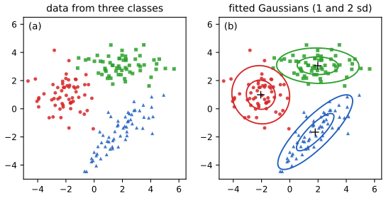
p. 323 Take Gaussian class-conditional densities, \[ p(\bm x\given y=c,\bm\theta)=\N(\bm x\given\bm\mu_c,\Sigma_c), \tag{9.2} \] so that the class posterior is \[ p(y=c\given\bm x,\bm\theta)\propto\pi_c\,\N(\bm x\given\bm\mu_c,\Sigma_c). \tag{9.3} \] The denominator is dropped because it is the same for every class. This is Gaussian discriminant analysis (GDA). The parameters are \(\bm\theta=(\bm\pi,\{\bm\mu_c,\Sigma_c\})\).
9.2.1 Quadratic decision boundaries
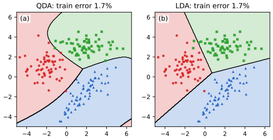
p. 324 Taking logarithms of (9.3) gives the discriminant function \[ \log p(y=c\given\bm x,\bm\theta)=\log\pi_c-\tfrac12\log|2\pi\Sigma_c|-\tfrac12(\bm x-\bm\mu_c)^\T\Sigma_c^{-1}(\bm x-\bm\mu_c)+\const. \tag{9.4} \] The boundary between two classes is the set where their discriminants agree, a quadratic equation in \(\bm x\) (a conic in the plane), so the method is called quadratic discriminant analysis (QDA). Figure 9.2a shows the boundaries fitted to the data of Figure 9.1.
Filling the gap 9.1: the boundary is a quadric, and what its shape tells you p. 324, (9.4)
Derivation
Write \[\delta_c(\bm x)=\log\pi_c-\frac12\log|\Sigma_c|-\frac12(\bm x-\bm\mu_c)^\T\Sigma_c^{-1}(\bm x-\bm\mu_c)\,;\] the term \(-\frac D2\log2\pi\) of (9.4) is the same for all classes and cancels in comparisons. Expanding the quadratic form and using the symmetry of \(\Sigma_c^{-1}\), \[ \delta_c(\bm x)-\delta_{c'}(\bm x)=-\tfrac12\bm x^\T\big(\Sigma_c^{-1}-\Sigma_{c'}^{-1}\big)\bm x+\bm x^\T\big(\Sigma_c^{-1}\bm\mu_c-\Sigma_{c'}^{-1}\bm\mu_{c'}\big)+k_{cc'}, \] \[ k_{cc'}=\log\frac{\pi_c}{\pi_{c'}}-\frac12\log\frac{|\Sigma_c|}{|\Sigma_{c'}|}-\frac12\bm\mu_c^\T\Sigma_c^{-1}\bm\mu_c+\frac12\bm\mu_{c'}^\T\Sigma_{c'}^{-1}\bm\mu_{c'}. \] The boundary between \(c\) and \(c'\) is \(\{\bm x:\delta_c=\delta_{c'}\}\), the zero set of a polynomial of degree at most two: a quadric. The quadratic part is \(\frac12(\Sigma_{c'}^{-1}-\Sigma_c^{-1})\); it is a non-zero matrix exactly when \(\Sigma_c\ne\Sigma_{c'}\) (an invertible map is injective), and then the boundary is genuinely curved. This matches the computation in the figure code, where the difference of two fitted discriminants equals this expression to machine precision.
One dimension. With \(D=1\), the class with the larger variance has the smaller \(-\frac12\log\sigma^2\) but a slower decay of \(-(x-\mu)^2/(2\sigma^2)\); for \(|x|\to\infty\) the quadratic term dominates, so the larger-variance class wins in both tails and the boundary consists of two points. Classifying "far from the data" is therefore not "no decision": QDA extrapolates the widest Gaussian, which is the curved lower-right boundary of Figure 9.2a that wraps around the blue class.
Regions. For \(C>2\) classes the region of class \(c\) is \(\bigcap_{c'\ne c}\{\delta_c\ge\delta_{c'}\}\), an intersection of quadric regions, which need not be convex or even connected.
See also (companion): ISL Section 4.4.3, QDA and the LDA and QDA demonstration.
9.2.2 Linear decision boundaries
p. 325 If the covariances are tied, \(\Sigma_c=\Sigma\) for all \(c\), the quadratic term of (9.4) is the same for every class: \[ \log p(y=c\given\bm x,\bm\theta)=\log\pi_c-\tfrac12(\bm x-\bm\mu_c)^\T\Sigma^{-1}(\bm x-\bm\mu_c)+\const \tag{9.5} \] \[ =\underbrace{\log\pi_c-\tfrac12\bm\mu_c^\T\Sigma^{-1}\bm\mu_c}_{\gamma_c}+\bm x^\T\underbrace{\Sigma^{-1}\bm\mu_c}_{\bm\beta_c}+\underbrace{\const-\tfrac12\bm x^\T\Sigma^{-1}\bm x}_{\kappa}, \tag{9.6} \] \[ =\gamma_c+\bm x^\T\bm\beta_c+\kappa. \tag{9.7} \] The last term does not depend on \(c\), so only \(\gamma_c+\bm\beta_c^\T\bm x\) matters: the discriminant is linear in \(\bm x\) and the boundaries are hyperplanes.
Filling the gap 9.2: expanding the square, the softmax form, and why the regions are polyhedra pp. 325–326, (9.5)–(9.8)
Derivation
Expansion. By symmetry of \(\Sigma^{-1}\), \[(\bm x-\bm\mu_c)^\T\Sigma^{-1}(\bm x-\bm\mu_c)=\bm x^\T\Sigma^{-1}\bm x-2\bm\mu_c^\T\Sigma^{-1}\bm x+\bm\mu_c^\T\Sigma^{-1}\bm\mu_c\,.\] Multiplying by \(-\frac12\) gives (9.6) with \(\kappa=\const-\frac12\bm x^\T\Sigma^{-1}\bm x\), which contains the normalising constant of the Gaussian (common to all classes since \(|\Sigma|\) is shared) and the quadratic term.
Softmax. Exponentiate (9.7) and normalise. The factor \(e^{\kappa}\) is common to numerator and denominator and cancels: \[ p(y=c\given\bm x,\bm\theta)=\frac{e^{\gamma_c+\bm\beta_c^\T\bm x}}{\sum_{c'}e^{\gamma_{c'}+\bm\beta_{c'}^\T\bm x}}=\frac{e^{\bm w_c^\T[1,\bm x]}}{\sum_{c'}e^{\bm w_{c'}^\T[1,\bm x]}},\qquad\bm w_c=[\gamma_c,\bm\beta_c], \tag{9.8} \] the multinomial logistic regression model. The Python code confirms numerically that the posterior of a fitted LDA equals the softmax of \(\bm\beta_c^\T\bm x+\gamma_c\) to machine precision.
Non-identifiability. Adding the same vector \(\bm v\) to every \(\bm w_c\) multiplies numerator and denominator by \(e^{\bm v^\T[1,\bm x]}\), so (9.8) is unchanged: only \(C-1\) of the weight vectors are free, and one is usually fixed at zero. In LDA this is visible in \(\bm\beta_c=\Sigma^{-1}\bm\mu_c\): shifting every mean by \(\bm m\) changes all \(\bm\beta_c\) by the same \(\Sigma^{-1}\bm m\) and leaves the classifier unchanged (it is just a translation of the data).
Regions. The class-\(c\) region is \[\{\bm x:(\bm w_c-\bm w_{c'})^\T[1,\bm x]\ge0\ \forall c'\ne c\}\], an intersection of half-spaces: a convex polyhedron. The \(C\) regions tile \(\R^D\) like the cells of a power diagram (with equal covariance \(\Sigma=\sigma^2I\) and equal priors they are the Voronoi cells of the means). In two dimensions three boundaries meet at one point (the triple point in Figure 9.2b), because the three pairwise equations \(\delta_1=\delta_2\), \(\delta_2=\delta_3\), \(\delta_1=\delta_3\) are linearly dependent.
9.2.3 The connection between LDA and logistic regression
pp. 325–326 Equation (9.8) has exactly the form of multinomial logistic regression. The difference is in how the weights are obtained: LDA first fits the Gaussians and the priors by maximising the joint likelihood \(p(\bm x,y\given\bm\theta)\) (Section 9.2.4) and then derives \(\bm w\) from \(\bm\theta\); logistic regression maximises the conditional likelihood \(p(y\given\bm x,\bm w)\) directly. In general the two give different weights (Exercise 10.3 of the book; see also Section 9.4 and Figure S1 below).
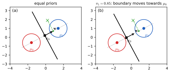
For two classes, (9.8) gives \[ p(y=1\given\bm x,\bm\theta)=\frac{e^{\bm\beta_1^\T\bm x+\gamma_1}}{e^{\bm\beta_1^\T\bm x+\gamma_1}+e^{\bm\beta_0^\T\bm x+\gamma_0}}=\frac{1}{1+e^{(\bm\beta_0-\bm\beta_1)^\T\bm x+(\gamma_0-\gamma_1)}}=\sigma\big((\bm\beta_1-\bm\beta_0)^\T\bm x+(\gamma_1-\gamma_0)\big). \tag{9.9, 9.10} \] With \[\gamma_1-\gamma_0=-\frac12(\bm\mu_1-\bm\mu_0)^\T\Sigma^{-1}(\bm\mu_1+\bm\mu_0)+\log\frac{\pi_1}{\pi_0}\] (9.11, 9.12) define \[ \bm w=\bm\beta_1-\bm\beta_0=\Sigma^{-1}(\bm\mu_1-\bm\mu_0),\tag{9.13} \] \[ \bm x_0=\tfrac12(\bm\mu_1+\bm\mu_0)-(\bm\mu_1-\bm\mu_0)\frac{\log(\pi_1/\pi_0)}{(\bm\mu_1-\bm\mu_0)^\T\Sigma^{-1}(\bm\mu_1-\bm\mu_0)}, \tag{9.14} \] so that \(\bm w^\T\bm x_0=-(\gamma_1-\gamma_0)\) and \[ p(y=1\given\bm x,\bm\theta)=\sigma\big(\bm w^\T(\bm x-\bm x_0)\big). \tag{9.15} \] The MAP rule is \(\hat y(\bm x)=1\) iff \(\bm w^\T\bm x>c\) with \(c=\bm w^\T\bm x_0\) (9.16); for equal priors \(c=\frac12\bm w^\T(\bm\mu_1+\bm\mu_0)\). If \(\Sigma=\sigma^2I\), then \(\bm w=\sigma^{-2}(\bm\mu_1-\bm\mu_0)\): classify by projecting onto the line joining the means and comparing with a threshold, the position of which depends on the prior (Figure 9.3). The prior only moves the threshold; it never changes the orientation of the boundary (the same is true for \(C>2\), where the priors enter only through the offsets \(\gamma_c\)).
Filling the gap 9.3: (9.11) to (9.16) step by step, the Bayes error, and how LDA and logistic regression relate pp. 325–326
Derivation
(9.11) to (9.15). From \(\gamma_c=\log\pi_c-\frac12\bm\mu_c^\T\Sigma^{-1}\bm\mu_c\), \[\gamma_1-\gamma_0=\log\frac{\pi_1}{\pi_0}-\frac12(\bm\mu_1^\T\Sigma^{-1}\bm\mu_1-\bm\mu_0^\T\Sigma^{-1}\bm\mu_0)\,,\] and the difference of quadratic forms factors because \(\Sigma^{-1}\) is symmetric: \[\bm\mu_1^\T\Sigma^{-1}\bm\mu_1-\bm\mu_0^\T\Sigma^{-1}\bm\mu_0=(\bm\mu_1-\bm\mu_0)^\T\Sigma^{-1}(\bm\mu_1+\bm\mu_0)\] (expand the product; the cross terms \(\bm\mu_1^\T\Sigma^{-1}\bm\mu_0\) and \(-\bm\mu_0^\T\Sigma^{-1}\bm\mu_1\) cancel). This is (9.12). With \(\bm w\) from (9.13) and \(\bm x_0\) from (9.14), \[ \bm w^\T\bm x_0=\tfrac12\bm w^\T(\bm\mu_1+\bm\mu_0)-\log\tfrac{\pi_1}{\pi_0}\cdot\frac{(\bm\mu_1-\bm\mu_0)^\T\Sigma^{-1}(\bm\mu_1-\bm\mu_0)}{(\bm\mu_1-\bm\mu_0)^\T\Sigma^{-1}(\bm\mu_1-\bm\mu_0)}=\tfrac12(\bm\mu_1-\bm\mu_0)^\T\Sigma^{-1}(\bm\mu_1+\bm\mu_0)-\log\tfrac{\pi_1}{\pi_0}=-(\gamma_1-\gamma_0), \] so \[(\bm\beta_1-\bm\beta_0)^\T\bm x+(\gamma_1-\gamma_0)=\bm w^\T\bm x-\bm w^\T\bm x_0=\bm w^\T(\bm x-\bm x_0)\,,\] which is (9.15). The denominator in (9.14) is \(\Delta^2>0\), where \[\Delta=\sqrt{(\bm\mu_1-\bm\mu_0)^\T\Sigma^{-1}(\bm\mu_1-\bm\mu_0)}\] is the Mahalanobis distance between the means.
Rule and prior. \(\hat y=1\) iff \(p(y=1\given\bm x)>\frac12\) iff \(\sigma(\cdot)>\frac12\) iff \(\bm w^\T(\bm x-\bm x_0)>0\), i.e. (9.16). Moving \(\pi_1\) changes only \(\bm x_0\), by \(-\frac{\log(\pi_1/\pi_0)}{\Delta^2}(\bm\mu_1-\bm\mu_0)\): along the line of the means, and towards \(\bm\mu_0\) when \(\pi_1>\pi_0\). The boundary hyperplane \(\{\bm w^\T\bm x=\bm w^\T\bm x_0\}\) keeps its normal \(\bm w\), which is the claim. (Confirmed numerically: for priors 0.2 and 0.8 the computed shift equals \(-\log 4\,(\bm\mu_1-\bm\mu_0)/\Delta^2\).)
The Bayes error of two equal-covariance Gaussians. Take equal priors. Given class 0, \[z=\bm w^\T\bm x\sim\N(\bm w^\T\bm\mu_0,\bm w^\T\Sigma\bm w)=\N(\bm w^\T\bm\mu_0,\Delta^2)\] because \[\bm w^\T\Sigma\bm w=(\bm\mu_1-\bm\mu_0)^\T\Sigma^{-1}(\bm\mu_1-\bm\mu_0)\,.\] The threshold is \(\frac12\bm w^\T(\bm\mu_0+\bm\mu_1)\) and \(\bm w^\T\bm\mu_1-\bm w^\T\bm\mu_0=\Delta^2\), so the threshold is \(\Delta^2/2\) above the class-0 mean, i.e. \(\Delta/2\) standard deviations. Hence \[\Pr(\text{error}\given y=0)=1-\Phi(\Delta/2)=\Phi(-\Delta/2)\,,\] the same for class 1 by symmetry, and the total error is \[ \Phi(-\Delta/2). \] (A simulation with 800,000 points agrees with this to three decimals.) The error depends on the data only through the Mahalanobis separation \(\Delta\) of the means.
LDA versus logistic regression: same family, different estimators. The map \((\pi_1,\bm\mu_0,\bm\mu_1,\Sigma)\mapsto(\bm w,b)\) with \(b=-\bm w^\T\bm x_0\) is onto \(\R^D\times\R\) (take \(\Sigma=I\), \(\bm\mu_1-\bm\mu_0=\bm w\), and choose the priors or the position of the means to get any \(b\)), so the set of posteriors LDA can express equals the set logistic regression can express. LDA has many more parameters (\(1+2D+D(D+1)/2\) against \(D+1\)) and the map is many-to-one: it picks one point of each fibre by maximum joint likelihood. When the Gaussian model is true, the extra structure helps (Section 9.4 and gap 9.12). When it is false, the conditional MLE is the better estimator of the posterior (gap 9.12).
See also (companion): Bayesian and Probabilistic ML, Section 4.2.1 (the sigmoid and softmax from Gaussian class densities); ESL Section 4.4.5, logistic regression or LDA?; All of Statistics, Section 22.5.
9.2.4 Model fitting
pp. 326–327 The likelihood of the training set is \[ p(\mathcal D\given\bm\theta)=\prod_{n=1}^N\mathrm{Cat}(y_n\given\bm\pi)\prod_{c=1}^C\N(\bm x_n\given\bm\mu_c,\Sigma_c)^{\mathbb I(y_n=c)}, \tag{9.17} \] so the log likelihood separates into a term for \(\bm\pi\) and one term per class, \[ \log p(\mathcal D\given\bm\theta)=\Big[\sum_{n}\sum_c\mathbb I(y_n=c)\log\pi_c\Big]+\sum_{c=1}^C\Big[\sum_{n:y_n=c}\log\N(\bm x_n\given\bm\mu_c,\Sigma_c)\Big]. \tag{9.18} \] The maximum likelihood estimates are \[ \hat\pi_c=\frac{N_c}{N},\qquad\hat{\bm\mu}_c=\frac1{N_c}\sum_{n:y_n=c}\bm x_n,\qquad\hat\Sigma_c=\frac1{N_c}\sum_{n:y_n=c}(\bm x_n-\hat{\bm\mu}_c)(\bm x_n-\hat{\bm\mu}_c)^\T. \tag{9.19, 9.20} \] The \(\hat\Sigma_c\) can overfit (be badly conditioned or singular) when \(N_c\) is small compared with \(D\).
Filling the gap 9.4: the MLE of GDA, the tied covariance, and when the MLE exists pp. 326–327, (9.17)–(9.21)
Derivation
Separation. The parameters \(\bm\pi\) and \((\bm\mu_c,\Sigma_c)\) for different \(c\) occur in different terms of (9.18) and are not coupled by any constraint (apart from \(\sum\pi_c=1\), which involves \(\bm\pi\) only), so each term is maximised separately.
Priors. The first term is \(\sum_cN_c\log\pi_c\), the categorical log likelihood; by Gibbs' inequality (Chapter 4, gap 4.1) its maximiser on the simplex is \(\hat\pi_c=N_c/N\).
Means and covariances. The \(c\)-th term is the log likelihood of \(N_c\) i.i.d. draws from \(\N(\bm\mu_c,\Sigma_c)\); its maximiser is the sample mean and the \(1/N_c\) sample covariance (Chapter 4, gap 4.3). This gives (9.19), (9.20), and requires \(\hat\Sigma_c\succ0\), which holds with probability one under a continuous distribution when \(N_c\ge D+1\); with \(N_c\le D\) the scatter matrix has rank at most \(N_c-1<D\) and the likelihood is unbounded: no MLE exists.
Tied covariance (9.21). Impose \(\Sigma_c=\Sigma\). With the precision \(\Lambda=\Sigma^{-1}\) and \[\bm S_c=\sum_{n:y_n=c}(\bm x_n-\hat{\bm\mu}_c)(\bm x_n-\hat{\bm\mu}_c)^\T\,,\] the means still decouple (the quadratic form is minimised at \(\hat{\bm\mu}_c\) for every \(\Lambda\)) and \[ \ell(\Lambda)=\frac N2\log|\Lambda|-\frac12\Tr\Big(\Lambda\sum_c\bm S_c\Big)+\const. \] This is the same function as in the single-Gaussian case with the scatter \(\bm S\) replaced by the within-class scatter \(\bm S_W=\sum_c\bm S_c\), so the maximiser is \(\hat\Sigma=\bm S_W/N=\sum_c\frac{N_c}N\hat\Sigma_c\), (9.21): the prior-weighted average of the class covariances, pooling all samples. It exists iff \(\bm S_W\succ0\), which needs \(N-C\ge D\) (the pooled scatter has rank at most \(N-C\), the sum of the class ranks \(N_c-1\)). The tied estimate is therefore well defined in many cases where the class covariances are not, which is the practical reason for tying.
Parameter counts. Besides \(C-1\) free priors and \(CD\) means, the covariance part costs \(CD(D+1)/2\) parameters (QDA), \(D(D+1)/2\) (LDA), \(CD\) (diagonal, i.e. Gaussian naive Bayes) or \(D\) (tied diagonal). For \(C=3\), \(D=2\): 17, 11, 14 and 10 parameters in all, the numbers the demonstration shows.
9.2.4.1 Tied covariances
p. 327 Forcing \(\Sigma_c=\Sigma\) gives linear boundaries and a more reliable estimate, because all samples are pooled: \[ \hat\Sigma=\frac1N\sum_{c=1}^C\sum_{n:y_n=c}(\bm x_n-\hat{\bm\mu}_c)(\bm x_n-\hat{\bm\mu}_c)^\T. \tag{9.21} \]
9.2.4.2 Diagonal covariances
p. 327 Restricting each \(\Sigma_c\) to be diagonal reduces the parameters from \(O(CD^2)\) to \(O(CD)\): this is the naive Bayes assumption (Section 9.3), which scales to high dimensions but cannot represent correlations between features. Tying a diagonal matrix across classes as well gives "diagonal LDA" (Bickel and Levina 2004). Each variance is estimated from one feature's values alone, so it is well defined whenever \(N_c\ge2\) and the feature varies.
9.2.4.3 MAP estimation
p. 327 A full diagonal assumption is strong. The alternative is the MAP estimate of one shared full covariance under a conjugate prior (Section 4.5.2), which the book writes as a convex combination of the MLE and its diagonal, \[ \hat\Sigma_{\rm map}=\lambda\,\diag(\hat\Sigma_{\rm mle})+(1-\lambda)\hat\Sigma_{\rm mle}, \tag{9.22} \] where \(\lambda\in[0,1]\) controls the amount of regularisation. This is regularised discriminant analysis (RDA; Friedman 1989; Hastie, Tibshirani and Friedman 2009, p. 656 in the book's numbering). It interpolates between LDA (\(\lambda=0\)) and diagonal-covariance naive Bayes (\(\lambda=1\)).
Filling the gap 9.5: where (9.22) comes from, what it does to the spectrum, and how to choose \(\lambda\) p. 327, (9.22)
Derivation
It is an inverse-Wishart MAP. With the conjugate prior \(\Sigma\sim\mathrm{IW}(\bm\Psi,\nu)\) the posterior mode given the scatter \(\bm S\) of \(N\) points about their (estimated) mean is \(\hat\Sigma_{\rm map}=(\bm\Psi+\bm S)/(\nu+D+1+N)\) (Chapter 4, gap 4.5). Choose \(\bm\Psi=\breve N\,\diag(\hat\Sigma_{\rm mle})\) with \(\breve N=\nu+D+1\) and use \(\bm S=N\hat\Sigma_{\rm mle}\): \[ \hat\Sigma_{\rm map}=\frac{\breve N\diag(\hat\Sigma_{\rm mle})+N\hat\Sigma_{\rm mle}}{\breve N+N}=\lambda\diag(\hat\Sigma_{\rm mle})+(1-\lambda)\hat\Sigma_{\rm mle},\qquad\lambda=\frac{\breve N}{\breve N+N}. \] So (9.22) is a MAP estimate whose prior mode is the diagonal of the MLE ("empirical Bayes", because the prior is centred using the data), with prior strength \(\breve N\) pseudo-observations; \(\lambda\) shrinks to zero as \(N\) grows, the usual behaviour of a prior. For tied LDA, apply it to the pooled \(\hat\Sigma\) of (9.21).
Positive definiteness, even when \(N<D\). Let \(\hat\Sigma=\hat\Sigma_{\rm mle}\succeq0\) and \(s_{dd}\) its diagonal entries (the marginal variances), all positive if every feature varies. Then \[\hat\Sigma_\lambda=(1-\lambda)\hat\Sigma+\lambda\diag(s)\succeq\lambda\min_ds_{dd}\,I\succ0\] for every \(\lambda\in(0,1]\), because \((1-\lambda)\hat\Sigma\succeq0\). Consequently the log determinant and the inverse needed in (9.4) exist even where the MLE is singular. For an upper bound, \[s_{dd}=\bm e_d^\T\hat\Sigma\bm e_d\le\lambda_{\max}(\hat\Sigma)\,,\] so \[\lambda_{\max}(\hat\Sigma_\lambda)\le\lambda_{\max}(\hat\Sigma)\] and the condition number is at most \(\lambda_{\max}(\hat\Sigma)/(\lambda\min_ds_{dd})\), finite and decreasing as \(\lambda\) grows.
Effect on correlations. With \(\bm D=\diag(s)^{-1/2}\) and the sample correlation matrix \(\bm R=\bm D\hat\Sigma\bm D\), \[\bm D\hat\Sigma_\lambda\bm D=(1-\lambda)\bm R+\lambda\bm I\] (the diagonal is not changed). RDA therefore leaves the variances alone and multiplies every correlation by \(1-\lambda\): a shrinkage of correlations towards zero, which is the covariance-matrix analogue of ridge regression (Chapter 4, gap 4.6).
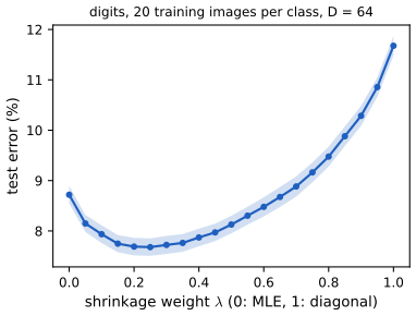
Choosing \(\lambda\). By cross-validation of the classification error. Figure S2 shows a case with \(D=64\) pixels and 20 training images per class (\(N=200\), so the pooled MLE is nearly singular): the test error is 8.7% at \(\lambda=0\), falls to 7.7% around \(\lambda=0.2\), and rises to 11.7% at \(\lambda=1\), where the correlations between neighbouring pixels are ignored. The sweet spot is a small positive \(\lambda\), a typical pattern when \(N\) is not large compared with \(D\).
See also (companion): ESL Section 4.3.1, regularised discriminant analysis (which shrinks each class covariance towards the pooled one); Chapter 4 of this course, Section 4.5.2.
9.2.5 Nearest centroid classifier
p. 328 With a uniform prior over classes and a shared covariance, the most probable class is the one whose mean is closest in squared Mahalanobis distance: \[ \hat y(\bm x)=\argmax_c\log p(y=c\given\bm x,\bm\theta)=\argmin_c(\bm x-\bm\mu_c)^\T\Sigma^{-1}(\bm x-\bm\mu_c). \tag{9.23} \] This is the nearest centroid (or nearest class mean, NCM) classifier. Replacing the distance by any other, \(\hat y=\argmin_cd^2(\bm x,\bm\mu_c)\) (9.24), one can learn a metric; the simple choice is a linear map, \[ d^2(\bm x,\bm\mu_c)=\|\bm x-\bm\mu_c\|_W^2=(\bm x-\bm\mu_c)^\T(\bm W\bm W^\T)(\bm x-\bm\mu_c)=\|\bm W^\T(\bm x-\bm\mu_c)\|^2, \tag{9.25} \] with the posterior \[ p(y=c\given\bm x,\bm\mu,\bm W)=\frac{\exp(-\frac12\|\bm W^\T(\bm x-\bm\mu_c)\|^2)}{\sum_{c'}\exp(-\frac12\|\bm W^\T(\bm x-\bm\mu_{c'})\|^2)}, \tag{9.26} \] and \(\bm W\in\R^{D\times K}\) is optimised by gradient descent on the discriminative loss (nearest class mean metric learning, Mensink et al. 2012). A new class needs only a single labelled prototype \(\bm\mu_c\), which makes the method usable for one-shot learning (the metric \(\bm W\) is learnt once).
Filling the gap 9.6: why (9.23) needs a tied covariance, the gradient for \(\bm W\), and convexity in \(\bm M=\bm W\bm W^\T\) pp. 328, (9.23)–(9.26)
Derivation
(9.23). With \(\pi_c=1/C\) the \(\log\pi_c\) in (9.5) is a constant, and the \(\kappa\) of (9.6) does not depend on \(c\), so \[\argmax_c\log p(y=c\given\bm x)=\argmax_c[-\frac12(\bm x-\bm\mu_c)^\T\Sigma^{-1}(\bm x-\bm\mu_c)]\]. The step uses the tied covariance: for class-specific \(\Sigma_c\), (9.4) also contains \(-\frac12\log|\Sigma_c|\) and a class-dependent metric, and the rule is no longer a nearest-centroid rule in any single metric. With \(\Sigma=\sigma^2I\) it is the usual Euclidean nearest-mean rule, and the decision regions are the Voronoi cells of the means. (The book's last equality in (9.25), \(\|\bm W(\bm x-\bm\mu_c)\|^2\), holds with \(\bm W\bm W^\T\) replaced by the symmetric \(\bm W^\T\bm W\); in the form written, \[(\bm x-\bm\mu)^\T\bm W\bm W^\T(\bm x-\bm\mu)=\|\bm W^\T(\bm x-\bm\mu)\|^2\,,\] as above.)
(9.26) is a softmax of the negative scaled distances, i.e. LDA's posterior (9.8) with \(\Sigma^{-1}=\bm W\bm W^\T\) and uniform priors (the terms \(\bm x^\T\bm W\bm W^\T\bm x\) cancel in the ratio).
Gradient. Put \(\bm d_c=\bm x-\bm\mu_c\), \[e_c=\frac12\|\bm W^\T\bm d_c\|^2=\frac12\bm d_c^\T\bm W\bm W^\T\bm d_c\] and \(\log p(y\given\bm x)=-e_y-\log\sum_{c}e^{-e_c}\). Since \(\partial e_c/\partial\bm W=\bm d_c\bm d_c^\T\bm W\), \[ \frac{\partial\log p(y\given\bm x)}{\partial\bm W}=-\bm d_y\bm d_y^\T\bm W+\sum_cp_c\,\bm d_c\bm d_c^\T\bm W=\sum_c\big(p_c-\mathbb I(c=y)\big)\bm d_c\bm d_c^\T\bm W,\qquad p_c=p(c\given\bm x). \] The data-fit term pulls the true class closer (\(-\bm d_y\bm d_y^\T\bm W\)) and the others are pushed away in proportion to their current probability. This expression matches a finite-difference derivative in the numerical experiment.
Convexity in \(\bm M\). In terms of the PSD matrix \(\bm M=\bm W\bm W^\T\), \(e_c=\frac12\Tr(\bm M\bm d_c\bm d_c^\T)\) is linear in \(\bm M\), and \(-\log p(y\given\bm x)=e_y+\log\sum_ce^{-e_c}\) is a linear function plus the log-sum-exp of linear functions of \(\bm M\), which is convex. The negative log likelihood is therefore convex in \(\bm M\) (on the convex cone of PSD matrices), although not in \(\bm W\): the non-convexity of metric learning is created by the factorisation \(\bm M=\bm W\bm W^\T\), not by the loss. A random-pair test of the convexity inequality in the code agrees.
See also (companion): shrunken centroids (nearest centroid with soft-thresholded means) in the Elements of Statistical Learning course.
9.2.6 Fisher's linear discriminant analysis *
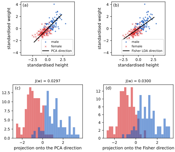
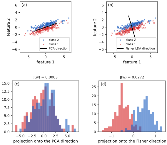
p. 328 Fitting a Gaussian with full covariance to high-dimensional data is hard. A different route is to reduce the dimension first, \(\bm z=\bm W^\T\bm x\) with \(\bm W\in\R^{D\times K}\) (the book writes \(\bm z=\bm W\bm x\) with \(\bm W\) of size \(K\times D\) here but \(\bm W^\T\bm S\bm W\) in (9.45); the second convention is used below), and then fit a Gaussian classifier in \(\R^K\). PCA (Section 20.1) picks the directions of largest variance irrespective of the labels, which can be exactly the wrong ones (Figure 9.4 and Figure S5). Fisher's linear discriminant analysis (FLDA) finds \(\bm W\) from an eigenproblem so that the projected classes are as well separated as possible. It always has \(K\le C-1\), whatever \(D\). FLDA is a hybrid of generative and discriminative: it uses class means and scatters (generative) to select directions by a criterion on class separation (discriminative).
9.2.6.1 Derivation of the optimal 1d projection
pp. 329–331 For two classes with means \(\bm\mu_1,\bm\mu_2\) put \(z_n=\bm w^\T\bm x_n\), \(m_k=\bm w^\T\bm\mu_k\) and \(s_k^2=\sum_{n:y_n=k}(z_n-m_k)^2\) (9.27, 9.28). Fisher's idea is to maximise the separation of the projected means relative to the spread within the projected classes, \[ J(\bm w)=\frac{(m_2-m_1)^2}{s_1^2+s_2^2}=\frac{\bm w^\T\bm S_B\bm w}{\bm w^\T\bm S_W\bm w}, \tag{9.29, 9.30} \] with the between-class and within-class scatter matrices \[ \bm S_B=(\bm\mu_2-\bm\mu_1)(\bm\mu_2-\bm\mu_1)^\T,\qquad\bm S_W=\sum_{n:y_n=1}(\bm x_n-\bm\mu_1)(\bm x_n-\bm\mu_1)^\T+\sum_{n:y_n=2}(\bm x_n-\bm\mu_2)(\bm x_n-\bm\mu_2)^\T. \tag{9.31, 9.32} \] Setting the derivative to zero gives the generalised eigenvalue problem \[ \bm S_B\bm w=\lambda\bm S_W\bm w,\qquad\lambda=\frac{\bm w^\T\bm S_B\bm w}{\bm w^\T\bm S_W\bm w}, \tag{9.36, 9.37} \] and if \(\bm S_W\) is invertible, \(\bm S_W^{-1}\bm S_B\bm w=\lambda\bm w\) (9.38). In the two-class case \(\bm S_B\bm w=(\bm\mu_2-\bm\mu_1)(m_2-m_1)\) is always parallel to \(\bm\mu_2-\bm\mu_1\), so (9.38) gives \(\bm w\propto\bm S_W^{-1}(\bm\mu_2-\bm\mu_1)\) (9.41), and since only the direction matters, \[ \bm w=\bm S_W^{-1}(\bm\mu_2-\bm\mu_1). \tag{9.42} \] If \(\bm S_W\propto\bm I\) this is the line joining the means.
Filling the gap 9.7: Exercise 9.1 in full, global optimality, and Fisher's direction is the LDA direction and a least-squares direction pp. 329–331, (9.30)–(9.42), p. 338
Derivation
(9.29) is (9.30). \(m_2-m_1=\bm w^\T(\bm\mu_2-\bm\mu_1)\) so \((m_2-m_1)^2=\bm w^\T\bm S_B\bm w\); and \[s_k^2=\sum_{n:y_n=k}\bm w^\T(\bm x_n-\bm\mu_k)(\bm x_n-\bm\mu_k)^\T\bm w\,,\] so \(s_1^2+s_2^2=\bm w^\T\bm S_W\bm w\) (the book's (9.33) to (9.35)).
Exercise 9.1: stationarity. Let \(a(\bm w)=\bm w^\T\bm S_B\bm w\), \(b(\bm w)=\bm w^\T\bm S_W\bm w\). For a symmetric matrix \(\bm A\), \(\nabla_{\bm w}\bm w^\T\bm A\bm w=2\bm A\bm w\) (the book's hint states it as \((\bm A+\bm A^\T)\bm w\)). The quotient rule gives \[ \nabla J=\frac{b\,\nabla a-a\,\nabla b}{b^2}=\frac{2}{b}\big(\bm S_B\bm w-J\,\bm S_W\bm w\big), \] which is zero iff \(\bm S_B\bm w=J(\bm w)\,\bm S_W\bm w\): (9.36), with \(\lambda=J(\bm w)=a/b\) (9.37). (The quotient is defined for \(b>0\), i.e. \(\bm w\ne0\) when \(\bm S_W\succ0\).)
The stationary point with the largest \(J\) is the global maximum. \(J\) is invariant to \(\bm w\mapsto t\bm w\), so it is a function on directions, and the sphere is compact; a maximum exists and is stationary. Put \(\bm v=\bm S_W^{1/2}\bm w\) (\(\bm S_W\succ0\)): \(J=\bm v^\T\bm M\bm v/\bm v^\T\bm v\) with \(\bm M=\bm S_W^{-1/2}\bm S_B\bm S_W^{-1/2}\), a Rayleigh quotient, whose maximum is \(\lambda_{\max}(\bm M)\), attained at the top eigenvector. The eigenvalues of \(\bm M\) coincide with those of \(\bm S_W^{-1}\bm S_B\) (they are similar), so the optimum is the top generalised eigenpair of (9.36); and every stationary \(\bm w\) is an eigenvector, with \(J\) equal to its eigenvalue.
Closed form for two classes. \(\bm S_B=\bm\delta\bm\delta^\T\) with \(\bm\delta=\bm\mu_2-\bm\mu_1\) has rank one, so \(\bm S_W^{-1}\bm S_B=(\bm S_W^{-1}\bm\delta)\bm\delta^\T\) has the single non-zero eigenvalue \(\bm\delta^\T\bm S_W^{-1}\bm\delta\) with eigenvector \(\bm S_W^{-1}\bm\delta\) (check: \[(\bm S_W^{-1}\bm\delta)\bm\delta^\T\bm S_W^{-1}\bm\delta=(\bm\delta^\T\bm S_W^{-1}\bm\delta)\bm S_W^{-1}\bm\delta\]). Hence (9.42) and \[ \max_{\bm w}J(\bm w)=(\bm\mu_2-\bm\mu_1)^\T\bm S_W^{-1}(\bm\mu_2-\bm\mu_1). \] A fine grid search over the angle of \(\bm w\) on the height and weight data finds the same maximiser and the same value.
Fisher's direction is LDA's direction. The tied covariance estimate is \(\hat\Sigma=\bm S_W/N\) (9.21), so the LDA weight vector (9.13) is \[\hat\Sigma^{-1}(\bm\mu_2-\bm\mu_1)=N\,\bm S_W^{-1}(\bm\mu_2-\bm\mu_1)\,,\] a positive multiple of (9.42). Fisher's criterion makes no Gaussian assumption; it recovers the Gaussian optimum direction. What LDA adds is the threshold (9.14) and the posterior probabilities.
Fisher's direction is also a least-squares direction. Regress the targets \(t_n=N/N_2\) (class 2) and \(t_n=-N/N_1\) (class 1), which sum to zero, on \(\bm x_n\) with an intercept. After centring the inputs, the normal equations for \(\bm w\) read \(\bm S_T\bm w=\sum_nt_n(\bm x_n-\bar{\bm x})\) with \[\bm S_T=\sum_n(\bm x_n-\bar{\bm x})(\bm x_n-\bar{\bm x})^\T=\bm S_W+\frac{N_1N_2}N\bm\delta\bm\delta^\T\] (gap 9.8). The right side is \[N_2\frac N{N_2}\bm\mu_2-N_1\frac N{N_1}\bm\mu_1-\bar{\bm x}\sum_nt_n=N\bm\delta\,.\] So \[\bm S_W\bm w=\bm\delta\,(N-\frac{N_1N_2}N\bm\delta^\T\bm w)\,;\] hence \(\bm w\) is a multiple \(\kappa\bm S_W^{-1}\bm\delta\), and substituting back, \[\kappa=N/(1+\frac{N_1N_2}N\bm\delta^\T\bm S_W^{-1}\bm\delta)>0\,.\] The least-squares coefficient vector is a positive multiple of Fisher's direction (numerically confirmed on the height and weight data). This is Bishop's observation (Section 4.1.5 of his book), here with the proof; note that only this target coding gives it.
See also (companion): Section 4.1.4, Fisher's linear discriminant and 4.1.5, its relation to least squares.
9.2.6.2 Extension to higher dimensions and multiple classes
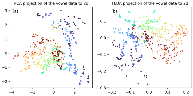
pp. 331–332 To project onto \(K\) dimensions, find \(\bm W\) with \(\bm z_n=\bm W^\T\bm x_n\) (see the remark above on the book's convention). With class means \(\bm m_c=\frac1{N_c}\sum_{n:y_n=c}\bm z_n\) and overall mean \(\bm m=\frac1N\sum_cN_c\bm m_c\) in the projected space define \[ \tilde{\bm S}_W=\sum_{c=1}^C\sum_{n:y_n=c}(\bm z_n-\bm m_c)(\bm z_n-\bm m_c)^\T,\qquad\tilde{\bm S}_B=\sum_{c=1}^CN_c(\bm m_c-\bm m)(\bm m_c-\bm m)^\T, \tag{9.43, 9.44} \] and maximise \[ J(\bm W)=\frac{|\tilde{\bm S}_B|}{|\tilde{\bm S}_W|}=\frac{|\bm W^\T\bm S_B\bm W|}{|\bm W^\T\bm S_W\bm W|}, \tag{9.45} \] where \(\bm S_W,\bm S_B\) are the same scatter matrices in the original space (\(\bm x_n\) for \(\bm z_n\), \(\bm\mu_c\) for \(\bm m_c\), \(\bm\mu\) for \(\bm m\)). The solution is \(\bm W=\bm S_W^{-1/2}\bm U\), where the columns of \(\bm U\) are the \(K\) leading eigenvectors of \(\bm S_W^{-1/2}\bm S_B\bm S_W^{-1/2}\) (if \(\bm S_W\) is singular, run PCA first). Footnote 2 offers the alternative criterion \(\Tr\{\tilde{\bm S}_W^{-1}\tilde{\bm S}_B\}\). The rank of \(\bm S_B\) is at most \(C-1\), so no more than \(K=C-1\) directions carry information. Figure 9.5 projects 10-dimensional vowel data (11 classes) to two dimensions.
Filling the gap 9.8: the scatter decomposition, rank \(C-1\), the determinant criterion, and FLDA with \(K=C-1\) equals LDA pp. 331–332, (9.43)–(9.45)
Derivation
Decomposition. Let \(\bm S_T=\sum_n(\bm x_n-\bm\mu)(\bm x_n-\bm\mu)^\T\). Write \(\bm x_n-\bm\mu=(\bm x_n-\bm\mu_c)+(\bm\mu_c-\bm\mu)\) for \(y_n=c\). The cross terms vanish because \(\sum_{n:y_n=c}(\bm x_n-\bm\mu_c)=0\), leaving \(\bm S_T=\bm S_W+\bm S_B\) with \(\bm S_B=\sum_cN_c(\bm\mu_c-\bm\mu)(\bm\mu_c-\bm\mu)^\T\) as in (9.44). For two classes this is \(\frac{N_1N_2}N\bm\delta\bm\delta^\T\), i.e. the book's (9.31) up to the factor \(N_1N_2/N\), which does not change the maximiser of \(J\).
Rank. \(\bm S_B=\sum_cN_c\bm a_c\bm a_c^\T\) with \(\bm a_c=\bm\mu_c-\bm\mu\) and \(\sum_cN_c\bm a_c=N\bm\mu-N\bm\mu=0\), so the \(C\) vectors \(\bm a_c\) are linearly dependent and span at most \(C-1\) dimensions. Thus \(\operatorname{rank}\bm S_B\le C-1\), which is the "\(-1\)" of the book's remark that \(\bm\mu\) is a linear function of the \(\bm\mu_c\). The generalised eigenvalue problem therefore has at most \(C-1\) non-zero eigenvalues, whatever \(D\) (confirmed: for three classes in ten dimensions exactly two are non-zero; for the 11 vowel classes, ten).
Maximising (9.45). Assume \(\bm S_W\succ0\) and \(\bm W\) of rank \(K\). The criterion is unchanged under \(\bm W\mapsto\bm W\bm A\) for invertible \(\bm A\) (both determinants are multiplied by \(|\bm A|^2\)). Put \(\bm V=\bm S_W^{1/2}\bm W\); then \(J=|\bm V^\T\bm M\bm V|/|\bm V^\T\bm V|\) with \(\bm M=\bm S_W^{-1/2}\bm S_B\bm S_W^{-1/2}\succeq0\), and replacing \(\bm V\) by an orthonormal basis of its column space (allowed by the invariance) we may assume \(\bm V^\T\bm V=\bm I_K\), so \(J=|\bm V^\T\bm M\bm V|\). By the Poincaré separation theorem (Cauchy interlacing), the eigenvalues \(\mu_1\ge\dots\ge\mu_K\) of \(\bm V^\T\bm M\bm V\) satisfy \(\mu_i\le\lambda_i(\bm M)\), where \(\lambda_1\ge\lambda_2\ge\dots\) are the eigenvalues of \(\bm M\). Hence \[ J=\prod_{i=1}^K\mu_i\le\prod_{i=1}^K\lambda_i(\bm M)\] (the \(\mu_i\ge0\) since \(\bm M\succeq0\)), with equality when the columns of \(\bm V\) are the top-\(K\) eigenvectors \(\bm U\) of \(\bm M\). So \(\bm W=\bm S_W^{-1/2}\bm U\) (up to \(\bm W\mapsto\bm W\bm A\)) maximises (9.45), and the maximum is \(\prod_{i\le K}\lambda_i\); the generalised eigenvectors normalised by \(\bm W^\T\bm S_W\bm W=\bm I\) are exactly these \(\bm W\) (up to rotation of the columns). The code confirms the maximum against 2,000 random projections. The same bound with sums gives, for footnote 2's \[\Tr\{(\bm W^\T\bm S_W\bm W)^{-1}\bm W^\T\bm S_B\bm W\}=\Tr(\bm V^\T\bm M\bm V)\le\sum_{i\le K}\lambda_i\]: the same \(\bm W\) maximises it. Because only the first \(C-1\) eigenvalues can be positive, \(K>C-1\) adds directions with zero criterion.
With \(K=C-1\), FLDA followed by nearest centroid is LDA. Under the tied covariance \(\hat\Sigma=\bm S_W/N\) and uniform priors, LDA classifies by the smallest \(\|\tilde{\bm x}-\tilde{\bm\mu}_c\|^2\), where \(\tilde{\bm x}=\bm S_W^{-1/2}\bm x\) (whitening; the factor \(N\) is common). The whitened means \(\tilde{\bm\mu}_c-\tilde{\bm\mu}\) span \(\mathcal R(\bm M)\) (since \(\bm M=\sum_cN_c\tilde{\bm a}_c\tilde{\bm a}_c^\T\)), of dimension at most \(C-1\), equal to the span of the top \(C-1\) eigenvectors \(\bm U\). Let \(\bm P=\bm U\bm U^\T\) project onto this span: \[\|\tilde{\bm x}-\tilde{\bm\mu}_c\|^2=\|\bm P(\tilde{\bm x}-\tilde{\bm\mu}_c)\|^2+\|(\bm I-\bm P)\tilde{\bm x}-(\bm I-\bm P)\tilde{\bm\mu}_c\|^2\,,\] and the second term equals the same quantity for every \(c\) (the whitened means differ from \(\tilde{\bm\mu}\) only inside the span). Therefore LDA depends on \(\bm x\) only through \(\bm U^\T\tilde{\bm x}=\bm W^\T\bm x\): it is nearest centroid, with the Euclidean metric, in the \((C-1)\)-dimensional discriminant coordinates. Choosing \(K<C-1\) gives reduced-rank LDA, which keeps the most discriminating \(K\) directions (Hastie, Tibshirani and Friedman 2009, Section 4.3.3); the vowel experiment of the code confirms that the \(K=10\) projection followed by nearest centroid reproduces the full LDA predictions on all 462 test points.
See also (companion): Section 4.1.6, Fisher's discriminant for multiple classes; ESL Section 4.3.3, reduced-rank LDA and the reduced-rank LDA demonstration.
9.3 Naive Bayes classifiers
p. 332 Naive Bayes keeps Bayes' rule but replaces the Gaussian by a much simpler assumption: the features are conditionally independent given the class, \[ p(\bm x\given y=c,\bm\theta)=\prod_{d=1}^Dp(x_d\given y=c,\bm\theta_{dc}), \tag{9.46} \] so that the posterior is \[ p(y=c\given\bm x,\bm\theta)=\frac{p(y=c\given\bm\pi)\prod_{d=1}^Dp(x_d\given y=c,\bm\theta_{dc})}{\sum_{c'}p(y=c'\given\bm\pi)\prod_{d=1}^Dp(x_d\given y=c',\bm\theta_{dc'})}, \tag{9.47} \] with \(\bm\theta=(\bm\pi,\{\bm\theta_{dc}\})\). It is "naive" because features are rarely independent, even given the class, but the model has only \(O(CD)\) parameters and is therefore hard to overfit, and it often classifies well anyway (Domingos and Pazzani 1997; Hand and Yu 2001).
9.3.1 Example models
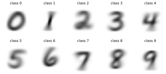
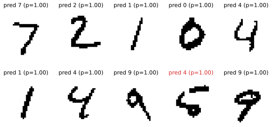
pp. 332–333 The factors in (9.46) depend on the type of feature. Binary features: \[p(\bm x\given y=c)=\prod_d\mathrm{Ber}(x_d\given\theta_{dc})\,,\] where \(\theta_{dc}\) is the probability that \(x_d=1\) in class \(c\) (the multivariate Bernoulli naive Bayes model). Categorical features \(x_d\in\{1,\dots,K\}\): \(\prod_d\mathrm{Cat}(x_d\given\bm\theta_{dc})\), with \(\theta_{dck}=p(x_d=k\given y=c)\). Real-valued features: \(\prod_d\N(x_d\given\mu_{dc},\sigma_{dc}^2)\), which is Gaussian discriminant analysis with diagonal covariance matrices. Figure 9.6 shows the Bernoulli parameters fitted to binarised MNIST digits, and Figure 9.7 some predictions; the book reports a test accuracy of 84.3% for this model.
9.3.2 Model fitting
pp. 333–334 The likelihood factorises over examples and, within an example, over features: \[ p(\mathcal D\given\bm\theta)=\prod_{n=1}^N\Big[\mathrm{Cat}(y_n\given\bm\pi)\prod_{d=1}^D\prod_{c=1}^Cp(x_{nd}\given\bm\theta_{dc})^{\mathbb I(y_n=c)}\Big], \tag{9.48, 9.49} \] \[ \log p(\mathcal D\given\bm\theta)=\Big[\sum_n\sum_c\mathbb I(y_n=c)\log\pi_c\Big]+\sum_{c=1}^C\sum_{d=1}^D\Big[\sum_{n:y_n=c}\log p(x_{nd}\given\bm\theta_{dc})\Big], \tag{9.50} \] a term for \(\bm\pi\) plus \(CD\) terms, one for each \((d,c)\) pair, that can be maximised separately (9.51). The estimates are: \(\hat\pi_c=N_c/N\); for categorical features \(\hat\theta_{dck}=N_{dck}/N_c\), with \(N_{dck}=\#\{n:x_{nd}=k,y_n=c\}\) (9.52); for binary features \(\hat\theta_{dc}=N_{dc}/N_c\), the fraction of class-\(c\) examples with feature \(d\) on (9.53); for real features \[ \hat\mu_{dc}=\frac1{N_c}\sum_{n:y_n=c}x_{nd},\qquad\hat\sigma^2_{dc}=\frac1{N_c}\sum_{n:y_n=c}(x_{nd}-\hat\mu_{dc})^2. \tag{9.54, 9.55} \] Fitting is therefore a matter of counting and averaging.
Filling the gap 9.9: why the naive Bayes MLE separates, and the zero-count problem pp. 333–334, (9.48)–(9.55)
Derivation
Separation. Exchanging the order of the products and using \(\mathbb I(y_n=c)\in\{0,1\}\), \[\prod_c p(x_{nd}\given\bm\theta_{dc})^{\mathbb I(y_n=c)}=p(x_{nd}\given\bm\theta_{d,y_n})\,;\] taking logarithms gives (9.50). Each parameter block \(\bm\theta_{dc}\) appears in exactly one term, the sum over \(\{x_{nd}:y_n=c\}\), and the blocks are variation independent (the only constraints are within a block, and \(\sum_c\pi_c=1\) within \(\bm\pi\)). The maximum of a sum of functions of disjoint variable sets is attained by maximising each separately.
Each term is the log likelihood of a one-dimensional sample, so the earlier solutions apply: the categorical (and Bernoulli) case is the multinomial MLE \(N_{dck}/N_c\) by Gibbs' inequality (Chapter 4, gap 4.1), the Gaussian case is Chapter 4, gap 4.2. In particular Gaussian naive Bayes equals GDA with the diagonal covariances \(\diag(\hat\sigma_{dc}^2)\): the two give identical posterior probabilities in the numerical experiment (and agree with scikit-learn's Gaussian naive Bayes).
Zero counts. If feature value \(k\) never occurs with class \(c\) in the training set, \(\hat\theta_{dck}=0\) and the likelihood of any test input with \(x_d=k\) is zero for class \(c\): a single unseen feature value vetoes the class, whatever the other features say (the demonstration with \(\alpha=0\) shows this). The Bayesian estimate of Section 9.3.3 fixes this.
9.3.3 Bayesian naive Bayes
pp. 334–335 For categorical features use the conjugate Dirichlet priors \[p(\bm\theta_{dc})=\mathrm{Dir}(\bm\theta_{dc}\given\breve{\bm\beta}_{dc})\,,\] with \(\breve\beta_{dck}\) pseudo-counts, and \(p(\bm\pi)=\mathrm{Dir}(\bm\pi\given\breve{\bm\alpha})\). The posterior is again a product of Dirichlets, \[ p(\bm\theta\given\mathcal D)=\mathrm{Dir}(\bm\pi\given\hat{\bm\alpha})\prod_{d=1}^D\prod_{c=1}^C\mathrm{Dir}(\bm\theta_{dc}\given\hat{\bm\beta}_{dc}),\qquad\hat\alpha_c=\breve\alpha_c+N_c,\ \hat\beta_{dck}=\breve\beta_{dck}+N_{dck}. \tag{9.56} \] The posterior predictive for the label is \[p(y=c\given\mathcal D)=\hat\alpha_c/\sum_{c'}\hat\alpha_{c'}\] and for a feature \[ p(x_d=k\given y=c,\mathcal D)=\bar\theta_{dck}=\frac{\hat\beta_{dck}}{\sum_{k'}\hat\beta_{dck'}}=\frac{\breve\beta_{dck}+N_{dck}}{\sum_{k'}(\breve\beta_{dck'}+N_{dck'})}, \tag{9.57} \] the posterior mean. With \(\breve\beta=0\) this is the MLE; with \(\breve\beta=1\) one adds one to every count (add-one or Laplace smoothing); for a binary feature \[ \bar\theta_{dc}=\frac{1+N_{dc1}}{2+N_{dc}}. \tag{9.58} \] Then \[ p(y=c\given\bm x,\mathcal D)\propto p(y=c\given\mathcal D)\prod_dp(x_d\given y=c,\mathcal D)=\bar\pi_c\prod_d\prod_k\bar\theta_{dck}^{\mathbb I(x_d=k)}, \tag{9.59} \] a fully Bayesian naive Bayes in which the parameters are integrated out; "plug in the posterior means" is exact here.
Filling the gap 9.10: the posterior (9.56), the predictive (9.59), and why plugging in the posterior mean is exact (for one test point) pp. 334–335, (9.56)–(9.59)
Derivation
Posterior. The likelihood, written in counts, is \(\prod_c\pi_c^{N_c}\prod_{d,c,k}\theta_{dck}^{N_{dck}}\). The prior is a product of independent Dirichlets, \[\propto\prod_c\pi_c^{\breve\alpha_c-1}\prod_{d,c,k}\theta_{dck}^{\breve\beta_{dck}-1}\,.\] Their product is \[\propto\prod_c\pi_c^{\breve\alpha_c+N_c-1}\prod_{d,c,k}\theta_{dck}^{\breve\beta_{dck}+N_{dck}-1}\,,\] a product of Dirichlet kernels: the posterior is the product (9.56), so \(\bm\pi\) and all \(\bm\theta_{dc}\) remain independent a posteriori.
Predictive. For a new pair \((y,\bm x)\), \[p(y=c,\bm x\given\mathcal D)=\E[\pi_c\prod_d\theta_{dc,x_d}\given\mathcal D]\]. The factors involve different, posteriorly independent, random variables (one \(\pi_c\) and one \(\bm\theta_{dc}\) for each \(d\)), so the expectation of the product is the product of the expectations: \[\E[\pi_c]\prod_d\E[\theta_{dc,x_d}]=\bar\pi_c\prod_d\bar\theta_{dc,x_d}\], using the Dirichlet mean \(\E[\theta_k]=\beta_k/\sum_{k'}\beta_{k'}\). Normalising over \(c\) gives (9.59). This is an exact integral, not a plug-in approximation.
Where the exactness stops. The factorisation uses that each parameter appears at most once in the integrand. For two test points \(\bm x,\bm x'\) of the same class the integrand contains \(\theta_{dck}\theta_{dck'}\), and \[\E[\theta_{dck}\theta_{dck'}]\ne\E[\theta_{dck}]\E[\theta_{dck'}]\] (the Dirichlet is not a product measure on its coordinates); the joint predictive of several test points is then not the product of single-point predictives. Predicting one point at a time, as in (9.59), is unaffected. (For a Dirichlet with parameters \(\beta_k\), total \(\beta_0\): \[\E[\theta_k\theta_{k'}]=\beta_k\beta_{k'}/(\beta_0(\beta_0+1))\], which differs from \(\E\theta_k\E\theta_{k'}=\beta_k\beta_{k'}/\beta_0^2\); a Monte Carlo check agrees.)
Laplace smoothing. For one Bernoulli feature, \(\bar\theta=(1+N_1)/(2+N)\) is the mean of the \(\mathrm{Beta}(1+N_1,1+N_0)\) posterior of a uniform prior, Laplace's rule of succession (Chapter 4, Section 4.6.2). It is strictly inside \((0,1)\) for any data, which removes the zero-count problem of gap 9.9. The pseudo-count is a bias that vanishes as \(N_c\to\infty\); on 1000 digits, MLE and add-one smoothing differ by about 0.5 percentage points in test accuracy (88.6% against 89.1%), with small pseudo-counts best (89.3% at \(\alpha=0.1\)) and \(\alpha=5\) over-smoothing (88.5%).
See also (companion): Chapter 4 of this course, Section 4.6.3 (the Dirichlet-multinomial model); Bayesian and Probabilistic ML, Section 4.2.3 (discrete features); ISL Section 4.4.4, naive Bayes.
9.3.4 The connection between naive Bayes and logistic regression
pp. 335–336 For discrete features with \(K\) states, let \(x_{dk}=\mathbb I(x_d=k)\) be a one-hot encoding. Then \(p(\bm x\given y=c)=\prod_d\prod_k\theta_{dck}^{x_{dk}}\) (9.60) and \[ p(y=c\given\bm x,\bm\theta)=\frac{\exp[\log\pi_c+\sum_d\sum_kx_{dk}\log\theta_{dck}]}{\sum_{c'}\exp[\log\pi_{c'}+\sum_d\sum_kx_{dk}\log\theta_{dc'k}]}=\frac{e^{\bm\beta_c^\T\bm x+\gamma_c}}{\sum_{c'}e^{\bm\beta_{c'}^\T\bm x+\gamma_{c'}}}, \tag{9.61, 9.62} \] with suitably defined \(\bm\beta_c,\gamma_c\): the form of multinomial logistic regression. Naive Bayes optimises the joint likelihood \(\prod_np(y_n,\bm x_n\given\bm\theta)\), logistic regression the conditional likelihood \(\prod_np(y_n\given\bm x_n,\bm\theta)\), so in general they give different fits (Exercise 10.3 of the book).
Filling the gap 9.11: the weights of the naive Bayes softmax, and "any exponential family" pp. 335–336, (9.60)–(9.62)
Derivation
Explicit weights. Index the entries of \(\bm x\) by the pair \((d,k)\). Then in (9.61) the exponent is \(\bm\beta_c^\T\bm x+\gamma_c\) with \[ \beta_{c,(d,k)}=\log\theta_{dck},\qquad\gamma_c=\log\pi_c. \] For binary features (\(K=2\), \(x_d\in\{0,1\}\)) one coordinate per feature is enough: \[\log\mathrm{Ber}(x_d\given\theta_{dc})=x_d\log\frac{\theta_{dc}}{1-\theta_{dc}}+\log(1-\theta_{dc})\,,\] so \[ \beta_{cd}=\log\frac{\theta_{dc}}{1-\theta_{dc}},\qquad\gamma_c=\log\pi_c+\sum_d\log(1-\theta_{dc}), \] the log-odds of each pixel and the sum of the "off" log probabilities (the code confirms that the Bernoulli naive Bayes posteriors on the digits equal this softmax to machine precision). In the two-class case the log odds are \[\log\frac{\pi_1}{\pi_0}+\sum_d[\log\frac{1-\theta_{d1}}{1-\theta_{d0}}+x_d\,\mathrm{LLR}_d]\]: each active feature adds its own log likelihood ratio, independently of the others. That is what the independence assumption means for the posterior.
Exponential families. Suppose each factor in (9.46) has the form \[p(x_d\given y=c)=h_d(x_d)\exp\{\bm\eta_{dc}^\T\bm T_d(x_d)-A_d(\bm\eta_{dc})\}\] with the same sufficient statistic \(\bm T_d\) in every class. Then \[\log p(y=c\given\bm x)=\log\pi_c-\sum_dA_d(\bm\eta_{dc})+\sum_d\bm\eta_{dc}^\T\bm T_d(x_d)+\sum_d\log h_d(x_d)-\log Z(\bm x)\,,\] and \(h_d\) is shared by the classes, so the posterior is a softmax of a function linear in the vector of sufficient statistics \((\bm T_d(x_d))_d\). The book's statement "holds for arbitrary exponential family" must be read that way: linear in \(\bm T(\bm x)\), not necessarily in \(\bm x\). For a Gaussian feature with class-independent variance \(\sigma_d^2\) the statistic is \(x_d\) and the posterior is linear in \(\bm x\) (diagonal LDA); with class-dependent variances it is linear in \((x_d,x_d^2)\), i.e. quadratic in \(\bm x\), in agreement with gap 9.1.
Same family, different fit. Every pair \((\bm\beta,\bm\gamma)\) that arises from some naive Bayes model is a softmax-logistic weight vector, and conversely any logistic weight can be matched by a naive Bayes model (for binary features and two classes, choose \(\theta_{d0}=\frac12\) and \(\theta_{d1}=\sigma(w_d)\), so that each log-odds difference is \(w_d\), and then pick \(\pi_1/\pi_0\) to match the intercept: the map is onto). Naive Bayes is thus a restricted estimator for the logistic model, one that uses closed-form counts and is valid with only a handful of examples, but is wrong when the independence assumption fails (gap 9.13).
See also (companion): ESL Section 4.4.5 (logistic regression or LDA?), which treats the same joint-versus-conditional comparison.
9.4 Generative vs discriminative classifiers
p. 336 A model \(p(\bm x,y)=p(y)p(\bm x\given y)\) is a generative classifier: it can produce examples \(\bm x\) of each class. A model of \(p(y\given\bm x)\) only is discriminative: it can only tell classes apart. The sections below weigh the two.
9.4.1 Advantages of discriminative classifiers
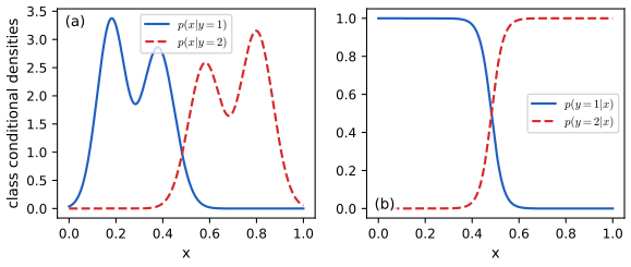
pp. 336–337 (i) Better predictive accuracy. The conditional \(p(y\given\bm x)\) is often much simpler than the joint, and the model does not have to spend capacity on the distribution of \(\bm x\) (Figure 9.8; Ng and Jordan 2002). (ii) Arbitrary feature preprocessing. Polynomial expansions, embeddings and so on can be used without having to model the correlated new features. (iii) Well-calibrated probabilities. Naive Bayes in particular makes strong independence assumptions and can produce probabilities extremely close to 0 or 1; logistic regression is usually better calibrated though it may still need adjustment (Niculescu-Mizil and Caruana 2005).
Filling the gap 9.12: what the joint and the conditional likelihood estimate in the limit, a model where logistic regression wins, and where LDA wins pp. 336–337, citing Ng and Jordan (2002)
Derivation
Two different limits. Let \((\bm x,y)\) be drawn from the true distribution \(P\) (not necessarily Gaussian). By the law of large numbers, maximising the joint log likelihood \(\frac1N\sum_n\log p_{\bm\theta}(\bm x_n,y_n)\) tends to maximising \(\E_P[\log p_{\bm\theta}(\bm x,y)]\), i.e. minimising \(\mathrm{KL}(P(\bm x,y)\|p_{\bm\theta}(\bm x,y))\); under regularity conditions the estimator converges to this joint KL projection \(\bm\theta_{\rm gen}^*\). The conditional MLE converges, in the same way, to the minimiser \(\bm\theta_{\rm dis}^*\) of the expected conditional KL \[\E_{P(\bm x)}\mathrm{KL}(P(y\given\bm x)\|p_{\bm\theta}(y\given\bm x))\,,\] i.e. of the expected conditional log loss \(L(\bm\theta)=-\E_P[\log p_{\bm\theta}(y\given\bm x)]\). When the model contains the truth, both limits give the true posterior (\(\mathrm{KL}=0\) is attained by both).
Misspecification: the discriminative limit is never worse in log loss. Let \(\mathcal F\) be the set of posteriors the linear-softmax model can express. By gap 9.2 (and gap 9.3) the posterior of an LDA model with any parameter \(\bm\theta\) lies in \(\mathcal F\). Logistic regression minimises \(L\) over all of \(\mathcal F\), so \(L(\bm\theta_{\rm dis}^*)\le L(\bm\theta_{\rm gen}^*)\): the population log loss of the logistic limit is at most that of the LDA limit, strictly smaller unless the LDA limit already minimises \(L\). (This concerns log loss; the 0-1 error need not be ordered in the same way, though for the examples here it is.)
A concrete failure of LDA. Let \(y\in\{0,1\}\) with equal priors and \(x\given y=c\sim\mathrm{Exp}(\lambda_c)\), \(\lambda_0=1\), \(\lambda_1=3\). Then \[\log\frac{p(y=1\given x)}{p(y=0\given x)}=\log\frac{\lambda_1}{\lambda_0}+(\lambda_0-\lambda_1)x\] is exactly linear in \(x\), so the posterior is exactly logistic with slope \(-2\), and logistic regression is consistent for it. LDA (Gaussian, tied variance) estimates in the limit \(\mu_0=1\), \(\mu_1=\frac13\), pooled variance \(\frac12(1+\frac19)=\frac59\), and so a slope \(w=(\mu_1-\mu_0)/\sigma^2=-\frac23\cdot\frac95=-1.2\), not \(-2\): LDA converges to the wrong function (and to a decision threshold in the wrong place). A sample of 800,000 points gives slopes \(-2.00\) and \(-1.20\) for logistic regression and LDA, as predicted.
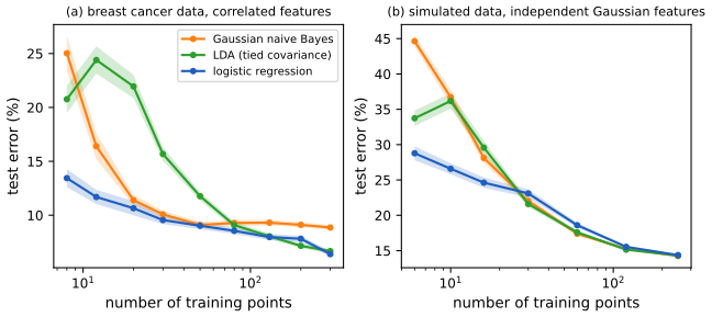
Where the generative classifier wins. If the generative model is correct, it is a smaller, more constrained model of the same posterior, and its maximum likelihood estimates are asymptotically more efficient than the conditional MLE (Efron 1975, for two Gaussian classes with a shared covariance: the asymptotic excess error of LDA is smaller than that of logistic regression), and Ng and Jordan (2002) show that naive Bayes approaches its (higher) asymptotic error with \(O(\log D)\) examples while logistic regression needs \(O(D)\). The price is exposure to misspecification. Figure S1 shows both regimes. In (a), real data with strongly correlated features, naive Bayes has a visibly higher plateau (about 9% against 6.5% for logistic regression). In (b), data for which the Gaussian independent-feature model is exactly true, LDA and naive Bayes are about 1.5 points better than logistic regression at 30 to 60 training points and the three coincide for large \(N\); for fewer than about 20 points (\(N\) comparable to \(D=10\)) logistic regression is the best, because the generative fits suffer from poorly estimated variances. So the "generative wins early" effect is real but modest and confined to a middle range of \(N\), not a universal law.
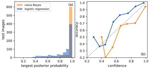
p. 337 On calibration: the maximum posterior probability of the naive Bayes model on the 797 test digits (8 × 8, binarised) exceeds 0.99 for 69% of the images, while its accuracy is 89%; logistic regression with its default L2 penalty gives more than 0.99 for only 18% of the images and is, if anything, slightly underconfident (mean confidence 86%, accuracy 92%).
Filling the gap 9.13: why naive Bayes is overconfident p. 337
Derivation
For two classes the naive Bayes log odds are \(\log\frac{\pi_1}{\pi_0}+\sum_d\mathrm{LLR}_d(x_d)\) (gap 9.11), a sum of one log likelihood ratio per feature. If features are conditionally independent given \(y\) this is exactly the log posterior odds. If, instead, feature 1 is repeated \(m\) times (exact copies), the true posterior odds still count that evidence once, but naive Bayes adds \(m\,\mathrm{LLR}_1\): the log odds from that feature are multiplied by \(m\). A numerical example in the code: a feature that is on with probability 0.2 in class 0 and 0.6 in class 1 has \(\mathrm{LLR}=\log3\); with \(m=5\) copies the naive Bayes log odds contain \(5\log3\), five times too strong.
More generally, with correlated features the same evidence is counted several times, so the log odds are inflated in magnitude and the posterior probabilities are pushed to 0 and 1, while the sign (hence the classification) is often still correct: which is why naive Bayes can be a good classifier and a bad probability model, as in Figure 9.7. Logistic regression fits the weights jointly, so duplicated features share a single total weight (with an L2 penalty, split equally), and no such inflation occurs.
9.4.2 Advantages of generative classifiers
p. 337 (i) Easy to fit. Naive Bayes needs counting and averaging, whereas logistic regression solves a convex optimisation (Section 10.2.3) and neural networks a non-convex one. (ii) Missing input features can be marginalised out (Section 9.4.3). (iii) Classes are fitted separately: adding a class does not require retraining the others, since the parameters of each class-conditional density are estimated on that class's data alone (Section 9.3.2 shows this for naive Bayes; for GDA the means and covariances of old classes are unchanged, though a tied covariance (9.21) would have to be updated). (iv) Unlabelled data can be used in semi-supervised learning through the marginal likelihood \(p(\bm x)=\sum_cp(\bm x,c)\), which has no analogue in a purely conditional model. (v) Robustness to spurious features. A discriminative model may latch onto features that separate the classes in the training set but not beyond it, while a generative model that captures the causal mechanism of the data can be more robust to distribution shift (the book's references: Arjovsky 2021; Zhou et al. 2021; Schölkopf 2019). These last claims are empirical or conceptual, not theorems.
9.4.3 Handling missing features
pp. 337–338 Suppose the value of \(x_1\) is missing at test time (and that its being missing carries no information about its value or the label). A generative classifier marginalises it out: \[ p(y=c\given\bm x_{2:D},\bm\theta)\propto p(y=c\given\bm\pi)\,p(\bm x_{2:D}\given y=c,\bm\theta)=p(y=c\given\bm\pi)\sum_{x_1}p(x_1,\bm x_{2:D}\given y=c,\bm\theta). \tag{9.63, 9.64} \] For Gaussian discriminant analysis the marginal of a sub-vector is Gaussian (Section 3.2.3): drop the corresponding entries of \(\bm\mu_c\) and the rows and columns of \(\Sigma_c\). Under the naive Bayes assumption the factor of the missing feature simply disappears, because \[ \sum_{x_1}p(x_1,\bm x_{2:D}\given y=c,\bm\theta)=\Big[\sum_{x_1}p(x_1\given\bm\theta_{1c})\Big]\prod_{d=2}^Dp(x_d\given\bm\theta_{dc})=\prod_{d=2}^Dp(x_d\given\bm\theta_{dc}). \tag{9.65} \] A discriminative model has no such principled rule, since it conditions on a complete \(\bm x\) (Section 1.5.5).
Filling the gap 9.14: the marginals, a classifier for every missingness pattern, and why imputation is worse pp. 337–338, (9.63)–(9.65)
Derivation
The marginal. Partition \(\bm x=(\bm x_o,\bm x_m)\) into observed and missing parts. If \(\bm x\sim\N(\bm\mu,\Sigma)\), then \(\bm x_o\sim\N(\bm\mu_o,\Sigma_{oo})\): the marginal of a Gaussian vector is Gaussian with the corresponding sub-vector and sub-matrix (integrate out \(\bm x_m\) with Section 3.2.3 of the book, or note that \(\bm x_o=\bm A\bm x\) with a selection matrix \(\bm A\) is a linear map and \(\bm A\Sigma\bm A^\T=\Sigma_{oo}\)). A numerical integration over the missing coordinate in two dimensions agrees with the sub-block formula to 6 digits. Hence \[ p(y=c\given\bm x_o)\propto\pi_c\,\N(\bm x_o\given\bm\mu_{c,o},\Sigma_{c,oo}), \] which is again of the form (9.3), with a sub-vector: for tied \(\Sigma\), still LDA, in the lower-dimensional space and with \(\Sigma_{oo}\) as covariance (and note: not \((\Sigma^{-1})_{oo}\), the corresponding block of the precision matrix). One fitted model thus yields a classifier for every one of the \(2^D\) missingness patterns, with no refitting.
(9.65). The sum over \(x_1\) factorises because (9.46) is a product and only one factor contains \(x_1\); the remaining factor is a normalised distribution and sums to one. The same holds for a continuous feature with an integral.
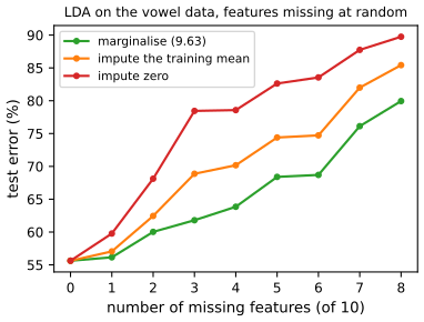
Why not impute? Replacing a missing coordinate by a fixed value, such as the overall mean or zero, evaluates the class-conditional density at an arbitrary point instead of integrating over it. For a missing coordinate the model's own answer for the class-conditional likelihood is the marginal; plugging in a constant does not average over the plausible values and can strongly favour the wrong class (the data point may lie far from the typical values of a class in the imputed coordinate). Figure S4 shows the effect on the vowel data (LDA, test error of 55.6% with all ten features): with 3 of 10 features missing, marginalising gives an error of 61.8%, mean imputation 68.9% and zero imputation 78.4%; the demonstration with 32 of 64 digit pixels hidden shows the same ordering (accuracy 70% against 56%).
Assumption. Marginalising is valid when the missingness mechanism is ignorable (missing completely at random or at random in Rubin's sense). If the probability that a feature is missing depends on its value, or on the class, the missingness itself is informative and \(p(\bm x_o\given y)\) is no longer the right quantity (compare the missing-data demonstration of Chapter 1).
See also (companion): Chapter 1 of this course, Section 1.5.5 and the missing-data demonstration; the Gaussian conditioning and marginal demo of Chapter 3.
9.5 Exercises
The one exercise of Chapter 9 (Murphy, 2022, p. 338), restated in my own words, with a complete solution (hidden).
Exercise 9.1 (derivation of Fisher's linear discriminant). Show that the maximum of \[J(\bm w)=\dfrac{\bm w^\T\bm S_B\bm w}{\bm w^\T\bm S_W\bm w}\] is attained where \(\bm S_B\bm w=\lambda\bm S_W\bm w\) with \[\lambda=\dfrac{\bm w^\T\bm S_B\bm w}{\bm w^\T\bm S_W\bm w}\,.\] (Hints: the derivative of a quotient is \((f'g-fg')/g^2\), and \(\frac{d}{d\bm x}\bm x^\T\bm A\bm x=(\bm A+\bm A^\T)\bm x\).)
Solution
Setting. \(\bm S_B\) and \(\bm S_W\) are symmetric, \(\bm S_B\succeq0\), \(\bm S_W\succ0\) (so the denominator is positive for \(\bm w\ne0\)). Let \(f(\bm w)=\bm w^\T\bm S_B\bm w\) and \(g(\bm w)=\bm w^\T\bm S_W\bm w\). Using the hint with \(\bm A=\bm S_B\) and \(\bm A=\bm S_W\) (symmetric, so \(\bm A+\bm A^\T=2\bm A\)), \(\nabla f=2\bm S_B\bm w\) and \(\nabla g=2\bm S_W\bm w\).
Stationarity. By the quotient rule applied coordinate by coordinate, \[ \nabla J=\frac{g\,\nabla f-f\,\nabla g}{g^2}=\frac{2}{g}\Big(\bm S_B\bm w-\frac fg\,\bm S_W\bm w\Big). \] At a maximum (an interior point of the open domain \(\bm w\ne0\)) the gradient vanishes, and since \(2/g\ne0\) this says \(\bm S_B\bm w=\lambda\bm S_W\bm w\) with \(\lambda=f/g=J(\bm w)\): (9.36) and (9.37). In words, the maximiser is a generalised eigenvector and the eigenvalue is the value of the criterion at it.
It is a maximum, and which eigenvector. \(J(t\bm w)=J(\bm w)\), so it suffices to consider the unit sphere, which is compact; \(J\) is continuous there, so a maximum exists and satisfies the stationarity equation. Every stationary point is a generalised eigenvector, with \(J\) equal to its eigenvalue, so the maximum value is the largest generalised eigenvalue, attained at the corresponding eigenvector. (Equivalently, with \(\bm v=\bm S_W^{1/2}\bm w\), \(J\) is the Rayleigh quotient of \(\bm S_W^{-1/2}\bm S_B\bm S_W^{-1/2}\), maximal at its top eigenvector.) When \(\bm S_W\) is invertible this is the ordinary eigenproblem \(\bm S_W^{-1}\bm S_B\bm w=\lambda\bm w\) (9.38).
Two-class check (numerical). For the height and weight data, the generalised eigenvector of \((\bm S_B,\bm S_W)\) with the largest eigenvalue is parallel to \(\bm S_W^{-1}(\bm\mu_2-\bm\mu_1)\), the gradient of \(J\) there has norm below \(10^{-5}\), the equation \(\bm S_B\bm w=J\bm S_W\bm w\) holds to 8 digits, and a search over 3,601 angles finds no direction with a larger \(J\). \(\square\)
Demonstrations
| Page | What it shows | In the notes |
|---|---|---|
| LDA, QDA and naive Bayes boundaries | Three-class two-dimensional data; the covariance model (full, tied, diagonal, tied diagonal), the shrinkage weight of (9.22) and a prior tilt; decision regions, confidence, errors. Presets: 1 QDA; 2 LDA; 3 naive Bayes; 4 prior tilt; 5 shrinkage. | 9.2.1, 9.2.2, 9.2.4 |
| Fisher's linear discriminant | A rotating projection line, the histograms of the projected classes and \(J(\bm w)\) against the angle, with the PCA and Fisher directions marked, on height and weight data and on a set where PCA fails. Presets: 1 PCA; 2 Fisher; 3 PCA fails; 4 Fisher rescues it; 5 worst direction. | 9.2.6 |
| Naive Bayes for digits | Bernoulli naive Bayes on 8 × 8 digits: fitted pixel maps, Laplace smoothing, training-set size, the posterior for any test image, and pixels hidden at test time (marginalised or zero-filled). Presets: 1 smoothing; 2 MLE; 3 30 images; 4 marginalised; 5 zero-filled. | 9.3.3, 9.4.3 |
The Python code that produces every figure of this page is code/ch09_linear_discriminant_analysis.py (see the code index). Companion demos: linear classifiers, LDA and QDA, reduced-rank LDA.
Notes on the book
Points where the book is imprecise or wrong
- (9.25). The distance is written \[(\bm x-\bm\mu_c)^\T(\bm W\bm W^\T)(\bm x-\bm\mu_c)=\|\bm W(\bm x-\bm\mu_c)\|^2\,.\] For a non-square or non-symmetric \(\bm W\) the right-hand side should be \(\|\bm W^\T(\bm x-\bm\mu_c)\|^2\) (equivalently \(\bm W^\T\bm W\) on the left); the posterior (9.26) inherits the same slip (gap 9.6).
- Section 9.2.6 notation. The projection is introduced as \(\bm z=\bm W\bm x\) with \(\bm W\) of size \(K\times D\), but (9.45), the solution \(\bm W=\bm S_W^{-1/2}\bm U\) and the \(\bm W^\T\bm S\bm W\) forms need \(\bm W\) of size \(D\times K\) (so \(\bm z=\bm W^\T\bm x\)), while footnote 2 writes \(\bm W\bm S\bm W^\T\). The notes use \(D\times K\) throughout.
- (9.23). The nearest-centroid form with a single \(\Sigma\) requires the covariance to be tied (and the prior uniform); the text introduces it without saying that the class covariances must be equal (gap 9.6).
- (9.31) against (9.44). The two-class between-class scatter \(\bm S_B=(\bm\mu_2-\bm\mu_1)(\bm\mu_2-\bm\mu_1)^\T\) differs from the multi-class definition \(\sum_cN_c(\bm\mu_c-\bm\mu)(\bm\mu_c-\bm\mu)^\T\) by the factor \(N_1N_2/N\) when \(C=2\). The maximiser of \(J\) is unchanged, but the eigenvalue \(\lambda\) differs by that factor between the two sections (gap 9.8).
- Section 9.2.4.3 and (9.22). The estimate is called a MAP estimate, but the "prior" is centred at the diagonal of the data's own MLE, so it is an empirical-Bayes (data-dependent prior) construction, and the relation \(\lambda=\breve N/(\breve N+N)\) between \(\lambda\) and the prior strength is not given (gap 9.5).
- Section 9.3.3. "The predictive distribution can be obtained merely by plugging in the posterior mean parameters" is exact for a single test point only; for several test points that share a parameter the joint predictive does not factorise (gap 9.10).
- Section 9.3.4. The softmax form of the naive Bayes posterior "holds for arbitrary feature distributions in the exponential family" only as a function linear in the sufficient statistics of the features (not in \(\bm x\) itself), and only if the sufficient statistics and base measure are the same in every class (gap 9.11).
- Section 9.4.1. The claim that discriminative classifiers "are often much more accurate" is stated without qualification; the cited result (Ng and Jordan 2002) shows that the generative classifier can be better for small training sets and the discriminative one asymptotically, and Figure S1(b) shows a regime in which the generative models win (gap 9.12).
References
- Murphy, K. P. (2022). Probabilistic Machine Learning: An Introduction. MIT Press, Cambridge, MA. Chapter 9, pp. 323–338. probml.github.io/pml-book/book1.html.
- Bickel, P. J. and Levina, E. (2004). Some theory for Fisher's linear discriminant function, "naive Bayes", and some alternatives when there are many more variables than observations. Bernoulli, 10(6), 989–1010.
- Bishop, C. M. (2006). Pattern Recognition and Machine Learning. Springer, New York.
- Davis, C. (1990). Body image and weight preoccupation: a comparison between exercising and non-exercising women. Appetite, 15, 13–21 (source of the height and weight data in the R package carData).
- Domingos, P. and Pazzani, M. (1997). On the optimality of the simple Bayesian classifier under zero-one loss. Machine Learning, 29(2–3), 103–130.
- Efron, B. (1975). The efficiency of logistic regression compared to normal discriminant analysis. Journal of the American Statistical Association, 70(352), 892–898.
- Fisher, R. A. (1936). The use of multiple measurements in taxonomic problems. Annals of Eugenics, 7(2), 179–188.
- Friedman, J. H. (1989). Regularized discriminant analysis. Journal of the American Statistical Association, 84(405), 165–175.
- Hand, D. J. and Yu, K. (2001). Idiot's Bayes: not so stupid after all? International Statistical Review, 69(3), 385–398.
- Hastie, T., Tibshirani, R. and Friedman, J. (2009). The Elements of Statistical Learning, 2nd edition. Springer, New York.
- Horn, R. A. and Johnson, C. R. (2013). Matrix Analysis, 2nd edition. Cambridge University Press (Cauchy interlacing and the Poincaré separation theorem, Section 4.3).
- LeCun, Y., Bottou, L., Bengio, Y. and Haffner, P. (1998). Gradient-based learning applied to document recognition. Proceedings of the IEEE, 86(11), 2278–2324.
- Mensink, T., Verbeek, J., Perronnin, F. and Csurka, G. (2012). Metric learning for large scale image classification: generalizing to new classes at near-zero cost. European Conference on Computer Vision.
- Ng, A. Y. and Jordan, M. I. (2002). On discriminative vs. generative classifiers: a comparison of logistic regression and naive Bayes. Advances in Neural Information Processing Systems 14.
- Niculescu-Mizil, A. and Caruana, R. (2005). Predicting good probabilities with supervised learning. International Conference on Machine Learning.
- Rubin, D. B. (1976). Inference and missing data. Biometrika, 63(3), 581–592.
The numerical statements in the text (the linear form and the softmax of the LDA posterior, the binary threshold and its shift with the prior, the Bayes error \(\Phi(-\Delta/2)\), the maximum likelihood and regularised estimates, the Fisher direction, its maximum value and its equality with the least-squares direction, the generalised eigenvalues and the rank of the between-class scatter, the equivalence of FLDA with \(K=C-1\) and LDA, the naive Bayes estimates, the Bernoulli softmax, the exponential-distribution example, the duplicated-feature inflation, the marginalisation formulas and the answer to the exercise) were confirmed numerically.