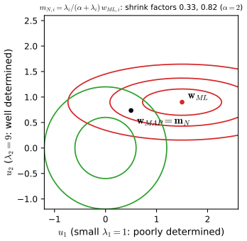
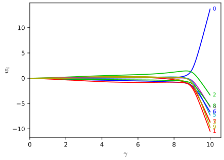
Regression predicts a continuous target from inputs. This chapter studies the simplest flexible family: models that are linear in their parameters but may be nonlinear in the inputs, through a fixed set of basis functions. Because the parameters enter linearly, everything is available in closed form: maximum likelihood is least squares (a projection), regularisation is a ridge or lasso penalty, the Bayesian posterior is Gaussian, the predictive distribution is Gaussian, and the marginal likelihood (the evidence) is an explicit determinant that can be maximised to set the regularisation strength from the training data alone. The chapter is also where the bias-variance trade-off and Bayesian model comparison first appear. Every step the book leaves to the reader is written out below.
They follow the book. Sections carry Bishop's numbers (3.1, 3.3.2, ...) and every displayed equation that appears in the book carries the book's own equation number, e.g. (3.15), so you can read these notes next to the book. Equations without a number are steps that the book skips.
Filling the gaps. Wherever the book says that a result "can be shown", is "easily verified", or is left as an exercise, an orange Filling the gap box or a proof gives the full argument. Proofs and derivations start hidden: open one with its bar, or use the button below.
Figures and demonstrations. The numerical figures of the chapter are reproduced from scratch by the Python code. The ▶ Demo boxes open an interactive demonstration already set to the case being discussed. Standard identities (matrix calculus, completing the square, the linear-Gaussian model, the Woodbury identity) are proved once in the mathematical toolkit.
Main reference
C. M. Bishop, Pattern Recognition and Machine Learning, Springer (2006), Chapter 3, pages 137–177. Section, equation, figure and exercise numbers below refer to this book. Further reading is listed in the references.
The explanations, derivations and code are my own; equations are cited by their numbers in the book.
The chapter at a glance
3.1 A linear basis function model \(y(\mathbf{x},\mathbf{w})\)\({}=\mathbf{w}^\T\bm\phi(\mathbf{x})\). With Gaussian noise, maximum likelihood is least squares, solved by the normal equations; geometrically the fit is the orthogonal projection of the target vector onto the span of the basis vectors. The noise precision is the inverse residual variance. Sequential (LMS) learning, ridge regression, the lasso and multiple outputs complete the section.
3.2 The expected squared loss splits into squared bias, variance and noise. Flexible models have low bias and high variance and rigid models the reverse; regularisation moves a model along this trade-off.
3.3 With a Gaussian prior the posterior over the weights is Gaussian (completing the square), the predictive distribution is Gaussian with a variance that shrinks as data arrive, and the predictive mean is a linear smoother with an equivalent kernel.
3.4 Models are compared through their marginal likelihood, which automatically penalises complexity; on average it favours the true model because an expected log Bayes factor is a KL divergence.
3.5 The evidence for a Gaussian linear model is explicit. Maximising it over the prior precision \(\alpha\) and the noise precision \(\beta\) gives re-estimation equations with an interpretable quantity \(\gamma\), the effective number of well-determined parameters.
3.6 Fixed basis functions suffer from the curse of dimensionality, which motivates the adaptive models of later chapters.
Notation. Inputs \(\mathbf{x}\), targets \(t\); \(\mathbf{X}=\{\mathbf{x}_n\}\), \(\mathbf{t}=(t_1,\dots,t_N)^\T\). \(\bm\phi(\mathbf{x})\)\({}=(\phi_0(\mathbf{x}),\dots,\phi_{M-1}(\mathbf{x}))^\T\) with \(\phi_0\equiv1\); \(\bm\phi_n=\bm\phi(\mathbf{x}_n)\); \(\bm\Phi\) is the \(N\times M\) design matrix with \(\Phi_{nj}=\phi_j(\mathbf{x}_n)\) ((3.16)), whose \(j\)th column is written \(\bm\varphi_j\in\R^N\). \(\beta\) is the noise precision, \(\alpha\) the prior precision of the weights.
Prerequisites. Gaussian distributions and the linear-Gaussian model (toolkit), completing the square (toolkit), matrix calculus and traces (toolkit, traces), the Woodbury identity (toolkit), Lagrange multipliers (toolkit), the KL divergence and Jensen's inequality (toolkit), and polynomial curve fitting from Chapter 1.
Printings. The text used here is a corrected printing. Where Bishop's errata list corrects an equation or exercise of this chapter, the notes give the corrected form and a short Erratum note naming the original.
Derivations start hidden: click any bar to open one.
3.1 Linear basis function models
pp. 137–139 The goal of regression is to predict a continuous target \(t\) from a \(D\)-dimensional input \(\mathbf{x}\), after seeing \(N\) training pairs. The simplest model is linear in the inputs, \(y(\mathbf{x},\mathbf{w})=w_0+w_1x_1+\dots+w_Dx_D\) (3.1), which is far too restrictive. The key idea of the chapter is to stay linear in the parameters while making the model nonlinear in the inputs, by feeding \(\mathbf{x}\) through fixed nonlinear functions \(\phi_j\).
Definition 3.1 (linear basis function model) p. 138, (3.2), (3.3)
Given fixed basis functions \(\phi_0,\dots,\phi_{M-1}\) with the dummy basis function \(\phi_0(\mathbf{x})=1\), the model is
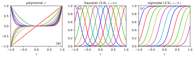
The weight \(w_0\) is the bias parameter (it lets the fitted function sit at the right height; it is not "bias" in the sense of Section 3.2). Common choices of \(\phi_j\) for a scalar input are the powers \(\phi_j(x)=x^j\), Gaussians \(\phi_j(x)=\exp\{-(x-\mu_j)^2/2s^2\}\) (3.4) and sigmoids \(\phi_j(x)=\sigma((x-\mu_j)/s)\) (3.5) with the logistic sigmoid \(\sigma(a)=1/(1+e^{-a})\) (3.6); here \(\mu_j\) set the locations and \(s\) the spatial scale. (Fourier, wavelet and other bases fit the same pattern.)
Figure 3.1 (reproduced). Examples of basis functions on \([-1,1]\): polynomials (left), Gaussians (3.4) (centre) and logistic sigmoids (3.5) (right). Polynomials are global (changing one weight changes the curve everywhere); Gaussians and sigmoids are local (a change of one weight affects a limited region, or, for sigmoids, one side of a step). Book: Figure 3.1, p. 139. Code: ch03_linear_regression.py, fig3_1. Download: PDF · SVG
Two remarks. First, "linear" means linear in \(\mathbf{w}\): the model can represent any function in the span of the \(\phi_j\), including highly nonlinear ones, and the learning problems below are convex. Second, the choice of basis is not unique in its effect on the parameters, but sometimes only in a trivial way. For instance, the logistic sigmoid and the hyperbolic tangent are related by \(\tanh a=2\sigma(2a)-1\), so a linear combination of sigmoids is a linear combination of \(\tanh\) functions with re-scaled weights and a shifted bias, and the two model families are the same set of functions (Exercise 3.1).
3.1.1 Maximum likelihood and least squares
pp. 140–143 Assume the target is a deterministic function plus Gaussian noise, \(t=y(\mathbf{x},\mathbf{w})+\epsilon\) (3.7), with \(\epsilon\sim\N(0,\beta^{-1})\), i.e.
Under squared loss the best prediction is the conditional mean, here \(\E[t\given\mathbf{x}]\)\({}=\int t\,p(t\given\mathbf{x})\,\d t\)\({}=y(\mathbf{x},\mathbf{w})\) (3.9). The Gaussian assumption makes the conditional distribution unimodal; mixtures of conditional Gaussians relax this (Section 14.5.1). For independent observations the likelihood (inputs are always conditioned on, never modelled) is
and setting it to zero gives the normal equations \(\bm\Phi^\T\bm\Phi\,\mathbf{w}\)\({}=\bm\Phi^\T\mathbf{t}\) with, when \(\bm\Phi^\T\bm\Phi\) is invertible,
\(\bm\Phi^\dagger\) is the Moore–Penrose pseudo-inverse. The log likelihood is concave in \(\mathbf{w}\), so this stationary point is the global maximum; it is unique exactly when the \(M\) columns of \(\bm\Phi\) are linearly independent (which needs \(N\ge M\)). Erratum. The book's (3.13) lacks the factor \(\beta\) on the right-hand side; it is restored above (it does not affect (3.14) or (3.15)).
Proof
Log likelihood. Taking logs in (3.10) and using \(\ln\N(t\given\mu,\beta^{-1})\)\({}=\tfrac12\ln\beta-\tfrac12\ln2\pi\)\({}-\tfrac\beta2(t-\mu)^2\) with \(\mu=\mathbf{w}^\T\bm\phi_n\), summed over \(n\), gives (3.11).
Gradient. With \(r_n(\mathbf{w})=t_n-\mathbf{w}^\T\bm\phi_n\) we have \(\nabla_{\mathbf{w}}r_n=-\bm\phi_n\), hence \(\nabla_{\mathbf{w}}E_D\)\({}=\sum_n r_n\nabla_{\mathbf{w}}r_n\)\({}=-\sum_n r_n\bm\phi_n\), and \(\nabla\ln p\)\({}=-\beta\nabla E_D\)\({}=\beta\sum_n r_n\bm\phi_n\) (written as a row vector this is (3.13)).
Normal equations. Setting the gradient to zero: \(\sum_n t_n\bm\phi_n\)\({}=\big(\sum_n\bm\phi_n\bm\phi_n^\T\big)\mathbf{w}\) (this is (3.14) after transposing). Now \(\sum_n\bm\phi_n\bm\phi_n^\T=\bm\Phi^\T\bm\Phi\) (the rows of \(\bm\Phi\) are \(\bm\phi_n^\T\)) and \(\sum_nt_n\bm\phi_n=\bm\Phi^\T\mathbf{t}\), so \(\bm\Phi^\T\bm\Phi\mathbf{w}=\bm\Phi^\T\mathbf{t}\).
Global maximum. The Hessian of \(\ln p\) is \(-\beta\bm\Phi^\T\bm\Phi\), and \(\mathbf{v}^\T\bm\Phi^\T\bm\Phi\mathbf{v}\)\({}=\|\bm\Phi\mathbf{v}\|^2\)\({}\ge0\), so \(\ln p\) is concave and every stationary point is a global maximiser. The Hessian is negative definite (maximiser unique) exactly when \(\bm\Phi\mathbf{v}=0\Rightarrow\mathbf{v}=0\), i.e. the columns of \(\bm\Phi\) are independent; then \(\bm\Phi^\T\bm\Phi\) is invertible and (3.15) follows. If the columns are dependent, the normal equations still have solutions (they form an affine subspace); the pseudo-inverse then picks the one of minimum norm (Filling the gap 3.2). ∎
Filling the gap 3.1: the role of the bias parameter p. 142, (3.18)–(3.20)
The book states the value of \(w_0\) without the steps, and says it "compensates for the difference between the averages". Here is why, and what it implies.
Derivation
Make the bias explicit: \(E_D(\mathbf{w})\)\({}=\tfrac12\sum_n\{t_n-w_0\)\({}-\sum_{j=1}^{M-1}w_j\phi_j(\mathbf{x}_n)\}^2\) (3.18). The derivative with respect to \(w_0\) is \(-\sum_n\{t_n-w_0\)\({}-\sum_{j\ge1}w_j\phi_j(\mathbf{x}_n)\}\); setting it to zero and dividing by \(N\),
Substituting back, the residual becomes \(t_n-w_0-\sum_{j\ge1}w_j\phi_j(\mathbf{x}_n)\)\({}=(t_n-\bar t)\)\({}-\sum_{j\ge1}w_j(\phi_j(\mathbf{x}_n)-\bar\phi_j)\). So the remaining weights solve an ordinary least-squares problem for centred targets and centred basis functions, and the bias is whatever makes the fitted function pass through the point of averages \((\bar\phi_1,\dots,\bar\phi_{M-1};\bar t)\). Two consequences: (i) the residuals at the optimum sum to zero, \(\sum_n r_n=0\) (this is the \(\phi_0\)-row of the normal equations \(\bm\Phi^\T\mathbf{r}=0\)); (ii) in regularised regression the bias should usually not be penalised, for otherwise the fit would depend on the arbitrary origin of \(t\) (Exercise 3.4). ∎
Result 3.2 (the maximum likelihood noise precision) pp. 142–143, (3.21)
the residual variance around the fitted regression function. It is biased: if the data really are generated by the model with true weights and noise precision \(\beta_0\), and \(\bm\Phi\) has full column rank, then \(\E[1/\beta_{\rm ML}]=\frac{N-M}{N}\,\beta_0^{-1}\). The unbiased version divides by \(N-M\); compare (3.95).
Proof
The maximisation over \((\mathbf{w},\beta)\) is done in two steps because \(\mathbf{w}_{\rm ML}\) does not depend on \(\beta\) (Result 3.1). For fixed \(\mathbf{w}=\mathbf{w}_{\rm ML}\), \(f(\beta)=\tfrac N2\ln\beta-\beta E_D\) has \(f'(\beta)=\tfrac N{2\beta}-E_D\) and \(f''(\beta)=-\tfrac N{2\beta^2}<0\), so \(f\) is concave with its unique maximum at \(\beta=N/(2E_D)\), which is (3.21).
Bias. Let \(\mathbf{t}=\bm\Phi\mathbf{w}^\star+\bm\epsilon\) with \(\bm\epsilon\sim\N(0,\beta_0^{-1}\mathbf{I}_N)\). The fitted vector is \(\bm\Phi\mathbf{w}_{\rm ML}=\mathbf{P}\mathbf{t}\), where \(\mathbf{P}\)\({}=\bm\Phi(\bm\Phi^\T\bm\Phi)^{-1}\bm\Phi^\T\) is the projection of Result 3.3. Since \(\mathbf{P}\bm\Phi=\bm\Phi\), the residual is \(\mathbf{t}-\mathbf{P}\mathbf{t}\)\({}=(\mathbf{I}-\mathbf{P})\bm\epsilon\). Using \(\mathbf{I}-\mathbf{P}\) symmetric and idempotent, \(\|(\mathbf{I}-\mathbf{P})\bm\epsilon\|^2\)\({}=\bm\epsilon^\T(\mathbf{I}-\mathbf{P})\bm\epsilon\), with expectation \(\beta_0^{-1}\Tr(\mathbf{I}-\mathbf{P})\)\({}=\beta_0^{-1}(N-\Tr\mathbf{P})\)\({}=\beta_0^{-1}(N-M)\) since \(\Tr\mathbf{P}\)\({}=\Tr[(\bm\Phi^\T\bm\Phi)^{-1}\bm\Phi^\T\bm\Phi]\)\({}=M\) (cyclic property of the trace, toolkit). Dividing by \(N\) gives the claim. Intuitively, fitting \(M\) weights uses up \(M\) degrees of freedom of the noise. ∎
3.1.2 Geometry of least squares
pp. 143–144 Think of \(\R^N\) with one axis per training point. The target vector \(\mathbf{t}=(t_1,\dots,t_N)^\T\) is a point of this space, and so is each basis function evaluated at the training inputs, \(\bm\varphi_j\)\({}=(\phi_j(\mathbf{x}_1),\dots,\phi_j(\mathbf{x}_N))^\T\), the \(j\)th column of \(\bm\Phi\) (the \(n\)th row is \(\bm\phi_n^\T\)). When \(MFigure 3.2 (redrawn). The least-squares solution as an orthogonal projection. The columns \(\bm\varphi_1,\bm\varphi_2\) of \(\bm\Phi\) span a subspace \(\mathcal S\) of \(\R^N\); the fitted vector \(\mathbf{y}=\bm\Phi\mathbf{w}_{\rm ML}\) is the foot of the perpendicular from \(\mathbf{t}\) to \(\mathcal S\). Book: Figure 3.2, p. 143.
Result 3.3 (least squares is an orthogonal projection) p. 143, (3.103); Exercise 3.2
Let \(\bm\Phi\) have independent columns and \(\mathbf{P}\)\({}=\bm\Phi(\bm\Phi^\T\bm\Phi)^{-1}\bm\Phi^\T\) (3.103). Then \(\mathbf{P}\) is symmetric and idempotent (\(\mathbf{P}^2=\mathbf{P}\)), \(\mathbf{P}\mathbf{v}\in\mathcal S\) for every \(\mathbf{v}\), and \(\mathbf{v}-\mathbf{P}\mathbf{v}\perp\mathcal S\); that is, \(\mathbf{P}\) is the orthogonal projector onto \(\mathcal S=\operatorname{col}(\bm\Phi)\). Consequently \(\mathbf{y}\)\({}=\bm\Phi\mathbf{w}_{\rm ML}\)\({}=\mathbf{P}\mathbf{t}\), the residual \(\mathbf{r}=\mathbf{t}-\mathbf{y}\) is orthogonal to every basis vector \(\bm\varphi_j\) (this is the normal equation \(\bm\Phi^\T\mathbf{r}=0\)), and \(\|\mathbf{t}\|^2\)\({}=\|\mathbf{y}\|^2+\|\mathbf{r}\|^2\).
Proof
Symmetry: \(\mathbf{P}^\T\)\({}=\bm\Phi[(\bm\Phi^\T\bm\Phi)^{-1}]^\T\bm\Phi^\T\)\({}=\mathbf{P}\) because \(\bm\Phi^\T\bm\Phi\) is symmetric. Idempotence: \(\mathbf{P}^2\)\({}=\bm\Phi(\bm\Phi^\T\bm\Phi)^{-1}[\bm\Phi^\T\bm\Phi](\bm\Phi^\T\bm\Phi)^{-1}\bm\Phi^\T\)\({}=\mathbf{P}\). Range: \(\mathbf{P}\mathbf{v}\)\({}=\bm\Phi[(\bm\Phi^\T\bm\Phi)^{-1}\bm\Phi^\T\mathbf{v}]\) is a combination of the columns. Orthogonality: for any \(\mathbf{u}=\bm\Phi\mathbf{c}\in\mathcal S\), \(\mathbf{u}^\T(\mathbf{v}-\mathbf{P}\mathbf{v})\)\({}=\mathbf{c}^\T(\bm\Phi^\T\mathbf{v}-\bm\Phi^\T\bm\Phi(\bm\Phi^\T\bm\Phi)^{-1}\bm\Phi^\T\mathbf{v})\)\({}=0\). Finally \(\bm\Phi\mathbf{w}_{\rm ML}\)\({}=\bm\Phi(\bm\Phi^\T\bm\Phi)^{-1}\bm\Phi^\T\mathbf{t}\)\({}=\mathbf{P}\mathbf{t}\), and Pythagoras applies to the orthogonal decomposition \(\mathbf{t}\)\({}=\mathbf{P}\mathbf{t}\)\({}+(\mathbf{I}-\mathbf{P})\mathbf{t}\). That the projection is the closest point of \(\mathcal S\): for any \(\mathbf{u}\in\mathcal S\), \(\|\mathbf{t}-\mathbf{u}\|^2\)\({}=\|\mathbf{t}-\mathbf{y}\|^2+\|\mathbf{y}\)\({}-\mathbf{u}\|^2\)\({}\ge\|\mathbf{t}-\mathbf{y}\|^2\) (the cross term vanishes since \(\mathbf{t}\)\({}-\mathbf{y}\perp\mathcal S\ni\mathbf{y}\)\({}-\mathbf{u}\)). ∎
Filling the gap 3.2: singular value decomposition, the pseudo-inverse and numerical trouble p. 143
The book remarks that solving the normal equations directly "can lead to numerical difficulties" when columns are nearly collinear, and that SVD cures this. Here is the content of that remark.
Derivation
Let \(\bm\Phi=\mathbf{U}\mathbf{\Sigma}\mathbf{V}^\T\) be the thin SVD with singular values \(s_1\ge\dots\ge s_r>0\), \(r=\operatorname{rank}\bm\Phi\), left vectors \(\mathbf{u}_i\in\R^N\) and right vectors \(\mathbf{v}_i\in\R^M\) (toolkit). Then \(\bm\Phi^\T\bm\Phi\)\({}=\mathbf{V}\mathbf{\Sigma}^2\mathbf{V}^\T\). When \(r=M\), \((\bm\Phi^\T\bm\Phi)^{-1}\bm\Phi^\T\)\({}=\mathbf{V}\mathbf{\Sigma}^{-2}\mathbf{V}^\T\mathbf{V}\mathbf{\Sigma}\mathbf{U}^\T\)\({}=\mathbf{V}\mathbf{\Sigma}^{-1}\mathbf{U}^\T\), so
For a rank-deficient \(\bm\Phi\) the same formula (sum over the \(r\) non-zero singular values) defines the Moore–Penrose pseudo-inverse \(\bm\Phi^\dagger\)\({}=\mathbf{V}_r\mathbf{\Sigma}_r^{-1}\mathbf{U}_r^\T\); it gives the solution of the normal equations of smallest norm, since any other solution adds a vector from the null space of \(\bm\Phi\), which is orthogonal to the span of the \(\mathbf{v}_i\) with \(i\le r\).
Why not the normal equations. Forming \(\bm\Phi^\T\bm\Phi\) squares the condition number: \(\kappa(\bm\Phi^\T\bm\Phi)\)\({}=s_1^2/s_r^2\)\({}=\kappa(\bm\Phi)^2\). With nearly collinear columns, \(s_r\) is tiny and the weights \(\mathbf{u}_r^\T\mathbf{t}/s_r\) become huge; a QR or SVD solve works with \(\kappa(\bm\Phi)\) instead.
Regularisation as a filter. For the ridge solution (3.28) below the same algebra gives \(\mathbf{w}\)\({}=\sum_i\frac{s_i}{s_i^2+\lambda}(\mathbf{u}_i^\T\mathbf{t})\mathbf{v}_i\) and fitted values \(\mathbf{y}\)\({}=\sum_i\frac{s_i^2}{s_i^2+\lambda}(\mathbf{u}_i^\T\mathbf{t})\mathbf{u}_i\): each component is multiplied by a shrinkage factor in \((0,1)\) that is close to 0 for small singular values, which is exactly how "the addition of a regularization term ensures that the matrix is non-singular". These factors return in Section 3.5.3 as the terms of \(\gamma\). ∎
3.1.3 Sequential learning
pp. 143–144 For large or streaming data sets we prefer to update the weights one observation at a time. If the error is a sum over data points, \(E=\sum_nE_n\), stochastic (sequential) gradient descent updates after presenting pattern \(n\) by \(\mathbf{w}^{(\tau+1)}\)\({}=\mathbf{w}^{(\tau)}-\eta\nabla E_n\) (3.22), with learning rate \(\eta>0\).
Algorithm 3.1 (least-mean-squares, LMS) p. 144, (3.23)
Initialise \(\mathbf{w}^{(0)}\) (for example \(0\)).
Present the training points one at a time (in order or at random). For point \(n\), with \(\bm\phi_n=\bm\phi(\mathbf{x}_n)\), compute the prediction error \(e_n=t_n-\mathbf{w}^{(\tau)\T}\bm\phi_n\) and update
\[ \mathbf{w}^{(\tau+1)}=\mathbf{w}^{(\tau)}+\eta\,\big(t_n-\mathbf{w}^{(\tau)\T}\bm\phi_n\big)\bm\phi_n. \tag{3.23} \]
Repeat until the weights stop changing.
Result 3.4 (the LMS update and when gradient descent converges) p. 144
(a) For \(E_n=\tfrac12(t_n-\mathbf{w}^\T\bm\phi_n)^2\) the update (3.22) is (3.23), and it multiplies the error on the presented point by \(1-\eta\|\bm\phi_n\|^2\). (b) Batch gradient descent \(\mathbf{w}\leftarrow\mathbf{w}-\eta\nabla E_D\) converges to \(\mathbf{w}_{\rm ML}\) from every start if and only if \(0<\eta<2/d_{\max}\), where \(d_{\max}\) is the largest eigenvalue of \(\bm\Phi^\T\bm\Phi\); the convergence rate is governed by the condition number \(d_{\max}/d_{\min}\). (c) Stochastic LMS with a constant \(\eta\) does not converge but hovers around \(\mathbf{w}_{\rm ML}\); \(\eta\) must be small (or decrease with \(\tau\) as in Robbins–Monro, \(\sum\eta_\tau=\infty,\ \sum\eta_\tau^2<\infty\)), which is what "chosen with care" in the book means.
Proof
(a) \(\nabla E_n\)\({}=-(t_n-\mathbf{w}^\T\bm\phi_n)\bm\phi_n\) gives (3.23). After the update the new residual on point \(n\) is \(t_n-\mathbf{w}'^\T\bm\phi_n\)\({}=(t_n-\mathbf{w}^\T\bm\phi_n)\)\({}-\eta(t_n-\mathbf{w}^\T\bm\phi_n)\|\bm\phi_n\|^2\)\({}=(1-\eta\|\bm\phi_n\|^2)(t_n-\mathbf{w}^\T\bm\phi_n)\). So \(\eta<1/\|\bm\phi_n\|^2\) makes the update shrink the error on the current point without overshooting.
(b) \(\nabla E_D\)\({}=\bm\Phi^\T\bm\Phi\mathbf{w}\)\({}-\bm\Phi^\T\mathbf{t}\)\({}=\bm\Phi^\T\bm\Phi(\mathbf{w}-\mathbf{w}_{\rm ML})\), so \(\mathbf{w}^{(\tau+1)}-\mathbf{w}_{\rm ML}\)\({}=(\mathbf{I}-\eta\bm\Phi^\T\bm\Phi)(\mathbf{w}^{(\tau)}-\mathbf{w}_{\rm ML})\). In the eigenbasis of \(\bm\Phi^\T\bm\Phi\) (eigenvalues \(d_i\ge0\)) each component is multiplied by \(1-\eta d_i\) per step. All components vanish iff \(|1-\eta d_i|<1\) for all \(i\), i.e. \(0<\eta<2/d_i\), i.e. \(\eta<2/d_{\max}\). The slowest component has factor \(1-\eta d_{\min}\); with \(\eta\) near \(2/d_{\max}\) the contraction per step is only about \(1-2d_{\min}/d_{\max}\).
(c) At \(\mathbf{w}_{\rm ML}\) the batch gradient vanishes but the individual \(\nabla E_n=-r_n\bm\phi_n\) do not (the residuals \(r_n\) are non-zero), so each step moves \(\mathbf{w}\) away by an amount proportional to \(\eta\); the weights therefore fluctuate with a spread that shrinks with \(\eta\). Decreasing step sizes with the stated conditions are the classical stochastic-approximation condition (Robbins and Monro, 1951; Section 2.3.5 of the book). ∎
The exact Bayesian counterpart of LMS, in which a matrix gain that shrinks as data accumulate replaces \(\eta\) and the batch answer is reproduced exactly after one pass, is the recursive update of Result 3.12.
3.1.4 Regularized least squares
pp. 144–147 To control over-fitting, add a penalty to the data error: minimise \(E_D(\mathbf{w})+\lambda E_W(\mathbf{w})\) (3.24), where \(\lambda\ge0\) sets the relative weight. The simplest penalty is \(E_W=\tfrac12\mathbf{w}^\T\mathbf{w}\) (3.25), known as weight decay in machine learning (because in sequential learning it pulls weights towards zero unless the data resist) and as ridge regression in statistics (Hoerl and Kennard, 1970). The total error is
which exists even when \(\bm\Phi^\T\bm\Phi\) is singular. As \(\lambda\to0\) it tends to \(\bm\Phi^\dagger\mathbf{t}\) and as \(\lambda\to\infty\) to \(0\). In the eigenbasis \(\{\mathbf{v}_i\}\) of \(\bm\Phi^\T\bm\Phi\) (eigenvalues \(d_i\)) the ridge coefficients are the least-squares ones multiplied by \(d_i/(d_i+\lambda)\in[0,1)\).
Proof
The gradient of (3.27) is \(-\bm\Phi^\T(\mathbf{t}-\bm\Phi\mathbf{w})\)\({}+\lambda\mathbf{w}\) and the Hessian is \(\bm\Phi^\T\bm\Phi+\lambda\mathbf{I}\), which is positive definite for \(\lambda>0\) (its eigenvalues are \(d_i+\lambda\ge\lambda\)). So the function is strictly convex, any stationary point is the unique global minimiser, and \((\bm\Phi^\T\bm\Phi+\lambda\mathbf{I})\mathbf{w}\)\({}=\bm\Phi^\T\mathbf{t}\) gives (3.28). In the eigenbasis, \(\mathbf{v}_i^\T\mathbf{w}\)\({}=\frac1{d_i+\lambda}\mathbf{v}_i^\T\bm\Phi^\T\mathbf{t}\) while the least-squares component is \(\frac1{d_i}\mathbf{v}_i^\T\bm\Phi^\T\mathbf{t}\) (when \(d_i>0\)); the ratio is \(d_i/(d_i+\lambda)\). ∎
Weight decay in a gradient step: \(\mathbf{w}\leftarrow\mathbf{w}\)\({}-\eta[\lambda\mathbf{w}-\bm\Phi^\T(\mathbf{t}-\bm\Phi\mathbf{w})]\)\({}=(1-\eta\lambda)\mathbf{w}\)\({}+\eta\bm\Phi^\T(\mathbf{t}-\bm\Phi\mathbf{w})\): the weights are multiplied by \(1-\eta\lambda<1\) before the data term acts. A further reading of the penalty, as the effect of adding noise to the inputs, is Exercise 3.4.
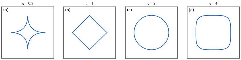
A more general penalty uses \(\tfrac\lambda2\sum_j|w_j|^q\) (3.29), with \(q=2\) giving (3.27). Figure 3.3 shows the contours of the penalty. The case \(q=1\) is the lasso (Tibshirani, 1996).
Figure 3.3 (reproduced). Contours of the regularisation term \(\sum_j|w_j|^q\) in (3.29) for \(q=0.5,1,2,4\). For \(q\ge1\) the penalty is convex; \(q=1\) has corners on the coordinate axes (a diamond), \(q=2\) is round, \(q=0.5\) is non-convex with spikes on the axes, and \(q\to\infty\) approaches a square. Book: Figure 3.3, p. 145. Code: ch03_linear_regression.py, fig3_3. Download: PDF · SVG
Result 3.6 (penalised and constrained least squares are equivalent) p. 145, (3.29), (3.30); Exercise 3.5
For \(\lambda>0\) let \(\mathbf{w}^\star(\lambda)\) minimise (3.29) and put \(\eta(\lambda)=\sum_j|w^\star_j(\lambda)|^q\). Then \(\mathbf{w}^\star(\lambda)\) minimises the unregularised error \(E_D\) of (3.12) subject to the constraint
\[ \sum_{j=1}^{M}|w_j|^q\le\eta. \tag{3.30} \]
Moreover \(\eta(\lambda)\) is non-increasing in \(\lambda\) (more penalty, smaller budget), \(\lambda\) is the Lagrange multiplier of the constraint, and for \(q\ge1\) (convex case) every binding constraint level \(\eta\in(0,\sum_j|w_{{\rm ML},j}|^q)\) arises from some \(\lambda\). For \(q<1\) the converse can fail because the constraint set is not convex.
Proof
Penalised implies constrained. Write \(R(\mathbf{w})=\sum_j|w_j|^q\). Suppose some \(\mathbf{w}\) with \(R(\mathbf{w})\le\eta(\lambda)\) had \(E_D(\mathbf{w})\({}+\tfrac\lambda2R(\mathbf{w})\({}+\tfrac\lambda2\eta(\lambda)\)\({}=E_D(\mathbf{w}^\star)\)\({}+\tfrac\lambda2R(\mathbf{w}^\star)\), contradicting that \(\mathbf{w}^\star\) minimises (3.29). (No convexity is needed in this direction.)
Lagrangian. The Lagrangian of "minimise \(E_D\) s.t. \(\tfrac12(R(\mathbf{w})-\eta)\le0\)" is \(E_D(\mathbf{w})\)\({}+\tfrac\lambda2(R(\mathbf{w})-\eta)\), which as a function of \(\mathbf{w}\) is (3.29) up to the constant \(-\lambda\eta/2\). By the KKT conditions (toolkit), at a solution with an active constraint \(\lambda\ge0\) and \(R(\mathbf{w}^\star)=\eta\), which is the formula for \(\eta(\lambda)\). For convex \(E_D\) and \(R\) (\(q\ge1\)) with \(\eta>0\) (so \(\mathbf{w}=0\) is strictly feasible, Slater's condition), the KKT conditions are also sufficient and a multiplier \(\lambda\) exists, which gives the converse.
Monotonicity. Let \(\lambda_1<\lambda_2\) with minimisers \(\mathbf{w}_1,\mathbf{w}_2\), \(R_i=R(\mathbf{w}_i)\), \(D_i=E_D(\mathbf{w}_i)\). Optimality of each for its own objective gives \(D_1+\tfrac{\lambda_1}2R_1\)\({}\le D_2+\tfrac{\lambda_1}2R_2\) and \(D_2+\tfrac{\lambda_2}2R_2\)\({}\le D_1+\tfrac{\lambda_2}2R_1\). Adding, \(\lambda_1R_1+\lambda_2R_2\)\({}\le\lambda_1R_2+\lambda_2R_1\), i.e. \((\lambda_2-\lambda_1)(R_1-R_2)\ge0\), so \(R_1\ge R_2\). The multiplier is the price of the budget: by the envelope theorem \(\lambda/2=-\d E_D^\star/\d\eta\). ∎
Filling the gap 3.3: why the lasso gives sparse solutions (Figure 3.4) pp. 145–146
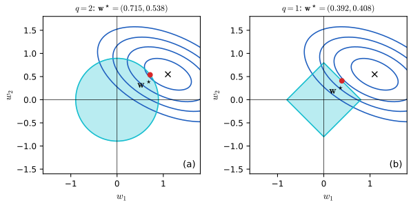
The book says the sparsity "can be seen from Figure 3.4". Here is the picture in formulas. The contours of \(E_D\) are ellipses centred at \(\mathbf{w}_{\rm ML}\) (it is a quadratic with Hessian \(\bm\Phi^\T\bm\Phi\)), and the solution of the constrained problem is the point where the smallest ellipse that meets the feasible region touches it. The \(q=2\) region is a disc, which has no preferred direction, so the touching point has no reason to lie on an axis. The \(q=1\) region is a diamond whose corners lie on the axes, and an ellipse reaches a corner more easily than a flat edge, so the touching point often has some coordinates exactly zero (as in the right panel, where \(w^\star_1=0\)).
Derivation
Optimality conditions. For the penalised problem with \(q=1\) the function is convex but not differentiable at \(w_j=0\); the minimiser satisfies \(0\in\partial E_D/\partial w_j\)\({}+\tfrac\lambda2\,\partial|w_j|\), where \(\partial|w_j|=\{{\rm sign}(w_j)\}\) if \(w_j\ne0\) and \([-1,1]\) at \(0\). Hence \(w^\star_j=0\) is allowed whenever \(\big|\partial E_D/\partial w_j(\mathbf{w}^\star)\big|\)\({}\le\lambda/2\): a whole interval of gradient values, so this happens with positive probability. For \(q=2\) the condition is \(\partial E_D/\partial w_j+\lambda w_j=0\), which at \(w_j=0\) demands the gradient to be exactly zero, an event of probability zero.
The orthonormal case in closed form. If \(\bm\Phi^\T\bm\Phi=\mathbf{I}\) then \(\mathbf{w}_{\rm ML}\)\({}=\bm\Phi^\T\mathbf{t}\)\({}\equiv\hat{\mathbf{w}}\) and, expanding, \(E_D(\mathbf{w})\)\({}=\text{const}+\tfrac12\|\mathbf{w}\)\({}-\hat{\mathbf{w}}\|^2\). The problem separates over coordinates: minimise \(\tfrac12(w-\hat w)^2+\tfrac\lambda2|w|^q\). For \(q=2\): \(w-\hat w+\lambda w=0\), so \(w=\hat w/(1+\lambda)\): proportional shrinkage, never exactly zero. For \(q=1\): \(w-\hat w+\tfrac\lambda2 s=0\) with \(s\in\partial|w|\). If \(w>0\) then \(w=\hat w-\lambda/2\), valid when \(\hat w>\lambda/2\); if \(w<0\), \(w=\hat w+\lambda/2\), valid when \(\hat w<-\lambda/2\); otherwise \(w=0\) (take \(s=2\hat w/\lambda\in[-1,1]\)). Together,
Every coefficient with \(|\hat w_j|\le\lambda/2\) is set to exactly zero and the others are shrunk by the constant \(\lambda/2\); increasing \(\lambda\) removes more of them, as the book says. ∎
Figure 3.4 (reproduced). Contours of the unregularised error (blue ellipses) with the constraint region (3.30) for the quadratic regulariser \(q=2\) (left, a disc) and the lasso \(q=1\) (right, a diamond). The optimum \(\mathbf{w}^\star\) is where the error contour first meets the region; for the lasso it sits on a corner with \(w_1^\star=0\), a sparse solution. In our computed illustration (region \(|w_1|^q+|w_2|^q\le0.8\)) the ridge optimum is \((0.715,0.538)\) and the lasso optimum is \((0.392,0.408)\). Book: Figure 3.4, p. 146. Code: ch03_linear_regression.py, fig3_4. Download: PDF · SVG
Regularisation lets complex models be trained on small data sets without severe over-fitting, but the problem of choosing model complexity is moved to choosing \(\lambda\) (or \(q\)). Sections 3.2 to 3.5 are about exactly this. The book then fixes the quadratic regulariser for the rest of the chapter.
3.1.5 Multiple outputs
pp. 146–147 For \(K>1\) targets \(\mathbf{t}\in\R^K\) one can share the same basis functions: \(\mathbf{y}(\mathbf{x},\mathbf{W})\)\({}=\mathbf{W}^\T\bm\phi(\mathbf{x})\) (3.31), with \(\mathbf{W}\) an \(M\times K\) matrix, and an isotropic Gaussian noise model \(p(\mathbf{t}\given\mathbf{x},\mathbf{W},\beta)\)\({}=\N(\mathbf{t}\given\mathbf{W}^\T\bm\phi(\mathbf{x}),\beta^{-1}\mathbf{I})\) (3.32). Stack the targets in an \(N\times K\) matrix \(\mathbf{T}\) whose \(n\)th row is \(\mathbf{t}_n^\T\). Then
Result 3.7 (multiple outputs decouple) p. 147, (3.34), (3.35); Exercise 3.6
The maximum likelihood weight matrix is \(\mathbf{W}_{\rm ML}\)\({}=(\bm\Phi^\T\bm\Phi)^{-1}\bm\Phi^\T\mathbf{T}\) (3.34), i.e. its \(k\)th column is \(\mathbf{w}_k=\bm\Phi^\dagger\mathbf{t}_k\) (3.35), where \(\mathbf{t}_k\) is the \(k\)th column of \(\mathbf{T}\). A single pseudo-inverse serves all outputs. The same is true for a general noise covariance \(\bm\Sigma\) (Exercise 3.6), because \(\bm\Sigma\) does not affect the mean parameters.
Proof
The squared norm splits over output components: \(\sum_n\|\mathbf{t}_n-\mathbf{W}^\T\bm\phi_n\|^2\)\({}=\sum_{k=1}^{K}\sum_n(t_{nk}-\mathbf{w}_k^\T\bm\phi_n)^2\)\({}=\sum_k\|\mathbf{t}_k-\bm\Phi\mathbf{w}_k\|^2\). So (3.33) is the sum of \(K\) separate single-output log likelihoods in \(\mathbf{w}_1,\dots,\mathbf{w}_K\) which share no parameters; each is maximised by Result 3.1, giving (3.35); stacking the columns gives (3.34). (In matrix form: \(\|\mathbf{T}-\bm\Phi\mathbf{W}\|_F^2\) has gradient \(-2\bm\Phi^\T(\mathbf{T}-\bm\Phi\mathbf{W})\) by matrix calculus, zero at (3.34).) The maximum over \(\beta\) is \(1/\beta_{\rm ML}\)\({}=\frac1{NK}\sum_n\|\mathbf{t}_n\)\({}-\mathbf{W}_{\rm ML}^\T\bm\phi_n\|^2\), by the same argument as Result 3.2 with \(NK\) in place of \(N\). ∎
From now on the book returns to a single target \(t\).
3.2 The bias-variance decomposition
pp. 147–152 Maximum likelihood over-fits flexible models, and limiting the number of basis functions limits flexibility; a regulariser seems to dissolve the dilemma but moves it to the choice of \(\lambda\). Minimising the regularised error over \(\lambda\) as well as \(\mathbf{w}\) is not an option, since it returns \(\lambda=0\). Before the Bayesian answer, the book gives the frequentist view of model complexity: the bias-variance trade-off.
Let \(h(\mathbf{x})\)\({}=\E[t\given\mathbf{x}]\)\({}=\int t\,p(t\given\mathbf{x})\,\d t\) (3.36) be the optimal prediction under squared loss (Section 1.5.5). For any prediction function \(y(\mathbf{x})\) the expected squared loss is
\[ \E[L]=\int\{y(\mathbf{x})-h(\mathbf{x})\}^2p(\mathbf{x})\,\d\mathbf{x}+\iint\{h(\mathbf{x})-t\}^2p(\mathbf{x},t)\,\d\mathbf{x}\,\d t. \tag{3.37} \]
Erratum. The book prints a single integral sign on the second term of (3.37), and likewise in (3.44); both are double integrals (over \(\mathbf{x}\) and \(t\)), as written here.
Filling the gap 3.4: where (3.37) comes from p. 148, (3.37)
The book quotes (3.37) from Section 1.5.5. For completeness, here is the two-line proof, which also shows that the second term is a floor no predictor can beat.
Integrate against \(p(\mathbf{x},t)\)\({}=p(t\given\mathbf{x})p(\mathbf{x})\). The cross term is \(2\int\{y(\mathbf{x})\)\({}-h(\mathbf{x})\}\Big[\int\{h(\mathbf{x})-t\}p(t\given\mathbf{x})\,\d t\Big]p(\mathbf{x})\,\d\mathbf{x}\), and the bracket is \(h(\mathbf{x})-\E[t\given\mathbf{x}]=0\) by (3.36). The first term does not depend on \(t\) once the \(t\)-integral of \(p(t\given\mathbf{x})\) (which is 1) is done, leaving \(\int\{y-h\}^2p(\mathbf{x})\,\d\mathbf{x}\). This is (3.37). The second term, the average conditional variance \(\int\var[t\given\mathbf{x}]\,p(\mathbf{x})\,\d\mathbf{x}\), is the irreducible noise; the first is minimised (to zero) by \(y=h\). ∎
The first term of (3.37) depends on the particular training set \(\mathcal D\) through \(y(\mathbf{x};\mathcal D)\). Our uncertainty about \(\mathcal D\) is handled by averaging over data sets drawn from \(p(\mathcal D)\), written \(\E_{\mathcal D}[\cdot]\).
Result 3.8 (bias-variance-noise decomposition) pp. 148–149, (3.38)–(3.44)
For a learning algorithm that returns \(y(\mathbf{x};\mathcal D)\) from the data set \(\mathcal D\),
The bias measures how far the average prediction over data sets is from the truth; the variance measures how much individual predictions scatter around that average; the noise is a property of the data, not of the model.
Proof
Fix \(\mathbf{x}\) and abbreviate \(y=y(\mathbf{x};\mathcal D)\), \(\bar y=\E_{\mathcal D}[y]\), \(h=h(\mathbf{x})\). Add and subtract \(\bar y\):
Take \(\E_{\mathcal D}\). The term \(\{\bar y-h\}^2\) is a constant with respect to \(\mathcal D\). The cross term is \(2\{\bar y-h\}\,\E_{\mathcal D}[y-\bar y]\)\({}=2\{\bar y-h\}(\bar y-\bar y)\)\({}=0\). This proves (3.40). Now average (3.37) over \(\mathcal D\) (the noise term does not involve \(\mathcal D\) as \(h\) and \(t\) refer to a fresh test point) and substitute (3.40) in its first term: integrating the two terms of (3.40) against \(p(\mathbf{x})\) gives (3.42) and (3.43), and the second term of (3.37) is (3.44). ∎
The trade-off: very flexible models have low bias and high variance, rigid models high bias and low variance, and the best predictor balances the two (the noise is a floor). Intuition from the polynomial example: a straight line fitted to a sine curve is always about the same wrong line (small variance, large bias), whereas a ninth-order polynomial follows each noisy data set, so the average over data sets is close to the truth but individual fits vary enormously.
Filling the gap 3.5: estimating bias and variance from simulated data sets pp. 149–151, (3.45)–(3.47)
The book generates \(L=100\) data sets \(\mathcal D^{(l)}\), each with \(N=25\) points from \(h(x)=\sin(2\pi x)\) plus noise, fits the model with 24 Gaussian basis functions and a bias parameter (\(M=25\)) and regularisation \(\lambda\) to each to get \(y^{(l)}(x)\), and then estimates the three terms. The estimators are Monte Carlo estimates of the integrals above.
Derivation
The expectation \(\E_{\mathcal D}[y(x;\mathcal D)]\) over data sets is estimated by the sample mean over the ensemble,
These are consistent as \(L\to\infty\) and \(N\to\infty\) by the law of large numbers. Two small points. (i) The variance estimator divides by \(L\), not \(L-1\), so it underestimates the true variance by the factor \((L-1)/L\) (1% for \(L=100\)); the bias estimator is slightly biased upwards for a similar reason: \(\E[\{\bar y-h\}^2]=\{\E y-h\}^2+\var(y)/L\). (ii) By construction the three quantities add up as in (3.41), so adding the noise level (known here: the standard deviation of the added noise is 0.3 in the book's data set, from Chapter 1) to (bias)\(^2\)+variance should track the test error on fresh data, which is how Figure 3.6 is checked. ∎
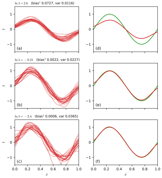
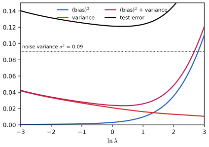
Figure 3.5 (reproduced). The dependence of bias and variance on model complexity, controlled by the regularisation coefficient \(\lambda\). \(L=100\) data sets, each of \(N=25\) points from \(\sin(2\pi x)\) plus noise; each is fitted with 24 Gaussian basis functions plus a bias (\(M=25\)) and the regulariser (3.27). Left: 20 of the 100 fits; right: their average (red) against the truth (green). Top row, \(\ln\lambda=2.6\) (large \(\lambda\)): the fits are alike (low variance) but the average is far from the sine (high bias). Bottom row, \(\ln\lambda=-2.4\) (small \(\lambda\)): the fits scatter widely (high variance) while their average follows the sine closely (low bias). Our values (squared bias, variance): \(\ln\lambda=2.6\): 0.0727, 0.0116; \(\ln\lambda=-0.31\): 0.0022, 0.0227; \(\ln\lambda=-2.4\): 0.0006, 0.0365. Book: Figure 3.5, p. 150. Code: ch03_linear_regression.py, fig3_5. Download: PDF · SVG
Figure 3.6 (reproduced). Squared bias, variance, their sum and the test-set error as functions of \(\ln\lambda\), for the ensemble of Figure 3.5. Small \(\lambda\) gives large variance and small bias, large \(\lambda\) the reverse; the sum has a minimum at an intermediate \(\lambda\), close to where the test error is smallest (the test error is computed as squared bias plus variance plus \(\sigma^2\) with \(\sigma=0.3\), so it sits above the book's curve, which implies a test-noise variance of about 0.05 that the book does not state). In our run squared bias plus variance is smallest at \(\ln\lambda=0.4\) (squared bias 0.0046, variance 0.0189). Book: Figure 3.6, p. 151. Code: ch03_linear_regression.py, fig3_6. Download: PDF · SVG
The decomposition for ridge regression, in closed form
For the ridge estimator the bias and variance can be computed exactly, which explains the shapes in Figure 3.6.
Result 3.9 (bias and variance of ridge regression) Section 3.2, complements Figures 3.5, 3.6
Fix the design \(\bm\Phi\) and suppose \(\mathbf{t}=\bm\Phi\mathbf{w}^\star+\bm\epsilon\) with \(\E\bm\epsilon=0\), \(\cov\bm\epsilon=\sigma^2\mathbf{I}\). Let \(\hat{\mathbf{w}}_\lambda\)\({}=(\bm\Phi^\T\bm\Phi+\lambda\mathbf{I})^{-1}\bm\Phi^\T\mathbf{t}\) and let \(d_i,\mathbf{v}_i\) be the eigenvalues and orthonormal eigenvectors of \(\bm\Phi^\T\bm\Phi\), \(w_i^\star=\mathbf{v}_i^\T\mathbf{w}^\star\). Then, in the coordinate along \(\mathbf{v}_i\),
and the expected in-sample prediction error (without the noise) is \(\frac1N\E\|\bm\Phi(\hat{\mathbf{w}}_\lambda-\mathbf{w}^\star)\|^2\)\({}=\frac1N\sum_id_i\Big[\frac{\lambda^2w_i^{\star2}}{(\lambda+d_i)^2}+\frac{\sigma^2d_i}{(\lambda+d_i)^2}\Big]\). The squared bias increases with \(\lambda\) from 0 (at \(\lambda=0\)) towards \(w_i^{\star2}\), and the variance decreases from \(\sigma^2/d_i\) towards 0.
Proof
Let \(\mathbf{B}\)\({}=(\bm\Phi^\T\bm\Phi+\lambda\mathbf{I})^{-1}\). Then \(\hat{\mathbf{w}}_\lambda\)\({}=\mathbf{B}\bm\Phi^\T\bm\Phi\mathbf{w}^\star\)\({}+\mathbf{B}\bm\Phi^\T\bm\epsilon\). The mean is \(\mathbf{B}\bm\Phi^\T\bm\Phi\mathbf{w}^\star\)\({}=\mathbf{B}(\bm\Phi^\T\bm\Phi+\lambda\mathbf{I}-\lambda\mathbf{I})\mathbf{w}^\star\)\({}=\mathbf{w}^\star\)\({}-\lambda\mathbf{B}\mathbf{w}^\star\), so the bias vector is \(-\lambda\mathbf{B}\mathbf{w}^\star\), with \(\mathbf{v}_i\)-component \(-\lambda w^\star_i/(d_i+\lambda)\). The covariance is \(\sigma^2\mathbf{B}\bm\Phi^\T\bm\Phi\mathbf{B}\)\({}=\sigma^2\mathbf{V}\operatorname{diag}\big(d_i/(d_i+\lambda)^2\big)\mathbf{V}^\T\), because \(\mathbf{B}\) and \(\bm\Phi^\T\bm\Phi\) share eigenvectors; this gives the variance along \(\mathbf{v}_i\). For the prediction error, \(\|\bm\Phi\mathbf{z}\|^2\)\({}=\sum_id_i(\mathbf{v}_i^\T\mathbf{z})^2\) and \(\E(\mathbf{v}_i^\T(\hat{\mathbf{w}}-\mathbf{w}^\star))^2\)\({}=\text{bias}_i^2+\text{variance}_i\). Monotonicity: \(\lambda/(\lambda+d_i)\) increases and \(d_i/(\lambda+d_i)^2\) decreases in \(\lambda\). ∎
The link with the Bayesian view
The frequentist decomposition needs many data sets, which in practice are not available (if they were, one would pool them into one big set and over-fit less). Bayesian inference replaces the average over hypothetical data sets by an average over parameters given the single observed set, and this section's trade-off survives in three precise ways.
Result 3.10 (the Bayesian choice \(\lambda=\alpha/\beta\) is the bias-variance optimum) Sections 3.2 and 3.3.1
(a) The posterior mean under the prior \(\N(\mathbf{w}\given0,\alpha^{-1}\mathbf{I})\) and noise precision \(\beta\) is the ridge estimator with \(\lambda=\alpha/\beta\) (Result 3.11). (b) Suppose the true weights are themselves drawn from that prior, \(\mathbf{w}^\star\sim\N(0,\alpha^{-1}\mathbf{I})\), and \(\sigma^2=\beta^{-1}\). Then the expected squared error of \(\hat{\mathbf{w}}_\lambda\) in direction \(\mathbf{v}_i\), averaged over both the noise and the prior (squared bias plus variance), is \(\dfrac{\lambda^2/\alpha+\sigma^2d_i}{(\lambda+d_i)^2}\), which is minimised in every direction simultaneously at \(\lambda=\sigma^2\alpha=\alpha/\beta\), where it equals \(1/(\alpha+\beta d_i)\), the \(i\)th eigenvalue of the posterior covariance \(\mathbf{S}_N\) of (3.54). (c) The predictive variance (3.59) is itself a decomposition of the same type: noise \(\beta^{-1}\) plus parameter uncertainty \(\bm\phi^\T\mathbf{S}_N\bm\phi\) (law of total variance).
Proof
(b) Average Result 3.9 over \(w_i^\star\) with \(\E w_i^{\star2}=1/\alpha\) (the components of \(\mathbf{w}^\star\) in any orthonormal basis are independent \(\N(0,\alpha^{-1})\)). Let \(f(\lambda)\)\({}=(\lambda^2/\alpha+\sigma^2d)/(\lambda+d)^2\). Then
\[ f'(\lambda)=\frac{2(\lambda/\alpha)(\lambda+d)-2(\lambda^2/\alpha+\sigma^2d)}{(\lambda+d)^3}=\frac{2d}{\alpha}\,\frac{\lambda-\sigma^2\alpha}{(\lambda+d)^3}, \]
which is negative for \(\lambda<\sigma^2\alpha\) and positive after, so the minimum is at \(\lambda=\sigma^2\alpha\) whatever \(d\) is. There \(f\)\({}=(\sigma^4\alpha+\sigma^2d)/(\sigma^2\alpha+d)^2\)\({}=\sigma^2/(\sigma^2\alpha+d)\)\({}=1/(\alpha+\beta d)\) with \(\sigma^2=1/\beta\). Because the optimal \(\lambda\) is the same for each \(i\), it also minimises the weighted sum in the prediction error. Equivalently, the sum over \(i\) is \(\Tr\mathbf{S}_N=\E\|\mathbf{w}-\mathbf{m}_N\|^2\), the Bayes risk of the posterior mean, which is minimal among all estimators.
(c) Given the data, \(t=\mathbf{w}^\T\bm\phi+\epsilon\) with \(\mathbf{w}\sim\N(\mathbf{m}_N,\mathbf{S}_N)\) and \(\epsilon\) independent. The law of total variance gives \(\var[t]\)\({}=\E_{\mathbf{w}}[\var(t\given\mathbf{w})]\)\({}+\var_{\mathbf{w}}[\E(t\given\mathbf{w})]\)\({}=\beta^{-1}+\bm\phi^\T\mathbf{S}_N\bm\phi\), which is (3.59). ∎
So the Bayesian treatment does not escape the trade-off, it resolves it: the prior says how large the true weights are expected to be, and that determines how much bias to accept in exchange for lower variance. When the prior is not known, Section 3.5 learns \(\alpha\) and \(\beta\) from the data, and so \(\lambda=\alpha/\beta\), without a validation set.
3.3 Bayesian linear regression
pp. 152–161 Maximum likelihood always prefers the more complex model, and hold-out data are wasteful. A Bayesian treatment places a prior on the weights, integrates over them, and thereby avoids over-fitting and gives a way to choose complexity from the training data alone. For simplicity there is one target; the extension to several follows Section 3.1.5.
3.3.1 Parameter distribution
pp. 152–156 Treat the noise precision \(\beta\) as a known constant for now. The likelihood (3.10) is the exponential of a quadratic function of \(\mathbf{w}\), so the conjugate prior is Gaussian: \(p(\mathbf{w})\)\({}=\N(\mathbf{w}\given\mathbf{m}_0,\mathbf{S}_0)\) (3.48).
Result 3.11 (the posterior over the weights) pp. 153–154, (3.49)–(3.55); Exercise 3.7
With prior (3.48) and likelihood (3.10), the posterior is Gaussian,
The mode equals the mean, so \(\mathbf{w}_{\rm MAP}=\mathbf{m}_N\). For the zero-mean isotropic prior \(p(\mathbf{w}\given\alpha)\)\({}=\N(\mathbf{w}\given0,\alpha^{-1}\mathbf{I})\) (3.52) this becomes
and \(\ln p(\mathbf{w}\given\mathbf{t})\)\({}=-\frac\beta2\sum_n\{t_n\)\({}-\mathbf{w}^\T\bm\phi_n\}^2\)\({}-\frac\alpha2\mathbf{w}^\T\mathbf{w}\)\({}+\text{const}\) (3.55). Hence the MAP weights are the ridge regression solution (3.28) with \(\lambda=\alpha/\beta\): \(\mathbf{m}_N\)\({}=(\frac\alpha\beta\mathbf{I}+\bm\Phi^\T\bm\Phi)^{-1}\bm\Phi^\T\mathbf{t}\). Special cases: if \(N=0\) the posterior is the prior; if the prior is infinitely broad, \(\mathbf{S}_0=\alpha^{-1}\mathbf{I}\) with \(\alpha\to0\), then \(\mathbf{m}_N\to\mathbf{w}_{\rm ML}\) (for full column rank).
Proof (completing the square)
By Bayes' theorem \(p(\mathbf{w}\given\mathbf{t})\)\({}\propto p(\mathbf{t}\given\mathbf{w})p(\mathbf{w})\). Keep only terms involving \(\mathbf{w}\):
With \(\mathbf{S}_N^{-1}:\)\({}=\mathbf{S}_0^{-1}+\beta\bm\Phi^\T\bm\Phi\) (symmetric positive definite) and \(\mathbf{m}_N:\)\({}=\mathbf{S}_N(\mathbf{S}_0^{-1}\mathbf{m}_0+\beta\bm\Phi^\T\mathbf{t})\), the identity \((\mathbf{w}-\mathbf{m}_N)^\T\mathbf{S}_N^{-1}(\mathbf{w}-\mathbf{m}_N)\)\({}=\mathbf{w}^\T\mathbf{S}_N^{-1}\mathbf{w}\)\({}-2\mathbf{w}^\T\mathbf{S}_N^{-1}\mathbf{m}_N\)\({}+\mathbf{m}_N^\T\mathbf{S}_N^{-1}\mathbf{m}_N\) shows the bracket equals \((\mathbf{w}-\mathbf{m}_N)^\T\mathbf{S}_N^{-1}(\mathbf{w}-\mathbf{m}_N)\) minus a term free of \(\mathbf{w}\). Hence \(\ln p\)\({}=-\frac12(\mathbf{w}-\mathbf{m}_N)^\T\mathbf{S}_N^{-1}(\mathbf{w}-\mathbf{m}_N)\)\({}+\const\), the kernel of \(\N(\mathbf{m}_N,\mathbf{S}_N)\); the constant is fixed by normalisation (toolkit). The same result follows from the linear-Gaussian formula (toolkit, book (2.116)) with prior \(\N(\mathbf{m}_0,\mathbf{S}_0)\), matrix \(\bm\Phi\) and noise precision \(\beta\).
For (3.55): set \(\mathbf{m}_0\)\({}=0,\ \mathbf{S}_0\)\({}=\alpha^{-1}\mathbf{I}\) in the display above. Maximising it is minimising \(\frac12\sum_n\{\cdot\}^2\)\({}+\frac{\alpha/\beta}2\mathbf{w}^\T\mathbf{w}\), i.e. (3.27) with \(\lambda=\alpha/\beta\); by Result 3.5, \(\mathbf{m}_N\)\({}=(\lambda\mathbf{I}+\bm\Phi^\T\bm\Phi)^{-1}\bm\Phi^\T\mathbf{t}\), which is also \(\beta\mathbf{S}_N\bm\Phi^\T\mathbf{t}\) since \(\beta\mathbf{S}_N\)\({}=(\frac\alpha\beta\mathbf{I}+\bm\Phi^\T\bm\Phi)^{-1}\). The limit \(\alpha\to0\) gives (3.15). ∎
A reading worth keeping: the Bayesian posterior mean is ridge regression with a specific, interpretable \(\lambda=\alpha/\beta\) (the ratio of the noise variance to the prior variance), and in addition the posterior supplies a covariance \(\mathbf{S}_N\), which is what the predictive distribution below uses.
Result 3.12 (sequential Bayesian updating and recursive least squares) p. 153; Exercises 3.8, 3.9
If the posterior after \(N\) points is \(\N(\mathbf{m}_N,\mathbf{S}_N)\), then after one more point \((\mathbf{x}_{N+1},t_{N+1})\) it is again Gaussian, with \(\bm\phi=\bm\phi(\mathbf{x}_{N+1})\),
This is the LMS update (3.23) with the scalar rate \(\eta\) replaced by the gain matrix \(\beta\mathbf{S}_{N+1}\) (precisely: \(\mathbf{m}_{N+1}\)\({}=\mathbf{m}_N\)\({}+\beta\mathbf{S}_{N+1}\bm\phi\,(t_{N+1}-\mathbf{m}_N^\T\bm\phi)\)). Processing the points one by one from the prior gives exactly the batch posterior (3.49), whatever the order.
Proof
Treat \(\N(\mathbf{w}\given\mathbf{m}_N,\mathbf{S}_N)\) as the prior and multiply by the likelihood of the new point, \(\propto\exp\{-\frac\beta2(t_{N+1}-\mathbf{w}^\T\bm\phi)^2\}\). The exponent, up to the factor \(-\frac12\), is \((\mathbf{w}-\mathbf{m}_N)^\T\mathbf{S}_N^{-1}(\mathbf{w}-\mathbf{m}_N)\)\({}+\beta(t_{N+1}-\mathbf{w}^\T\bm\phi)^2\)\({}=\mathbf{w}^\T(\mathbf{S}_N^{-1}+\beta\bm\phi\bm\phi^\T)\mathbf{w}\)\({}-2\mathbf{w}^\T(\mathbf{S}_N^{-1}\mathbf{m}_N+\beta\bm\phi\,t_{N+1})\)\({}+\const\), which has the same form as in the proof of Result 3.11, giving the first pair of formulas (Exercise 3.8). The linear-Gaussian route (Exercise 3.9) reads off the same formulas from (2.116) with \(\bm\Lambda=\mathbf{S}_N^{-1}\), \(\mathbf{A}=\bm\phi^\T\), \(\mathbf{L}=\beta\).
Gain form. Sherman–Morrison (Woodbury with rank one): \((\mathbf{S}_N^{-1}+\beta\bm\phi\bm\phi^\T)^{-1}\)\({}=\mathbf{S}_N\)\({}-\dfrac{\beta\mathbf{S}_N\bm\phi\bm\phi^\T\mathbf{S}_N}{1+\beta\bm\phi^\T\mathbf{S}_N\bm\phi}\)\({}=\mathbf{S}_N-\mathbf{k}\bm\phi^\T\mathbf{S}_N\), with \(\mathbf{k}\) as above (multiply numerator and denominator by \(\beta^{-1}\)). Also \(\mathbf{S}_{N+1}\bm\phi\)\({}=\mathbf{S}_N\bm\phi\)\({}-\dfrac{\beta\mathbf{S}_N\bm\phi(\bm\phi^\T\mathbf{S}_N\bm\phi)}{1+\beta\bm\phi^\T\mathbf{S}_N\bm\phi}\)\({}=\dfrac{\mathbf{S}_N\bm\phi}{1+\beta\bm\phi^\T\mathbf{S}_N\bm\phi}\)\({}=\beta^{-1}\mathbf{k}\), so \(\mathbf{k}=\beta\mathbf{S}_{N+1}\bm\phi\). Using \(\mathbf{S}_N^{-1}\)\({}=\mathbf{S}_{N+1}^{-1}-\beta\bm\phi\bm\phi^\T\) in the mean,
\[ \mathbf{m}_{N+1}=\mathbf{S}_{N+1}\mathbf{S}_{N+1}^{-1}\mathbf{m}_N-\beta\mathbf{S}_{N+1}\bm\phi\bm\phi^\T\mathbf{m}_N+\beta\mathbf{S}_{N+1}\bm\phi\,t_{N+1}=\mathbf{m}_N+\beta\mathbf{S}_{N+1}\bm\phi\,(t_{N+1}-\bm\phi^\T\mathbf{m}_N). \]
Order independence: after any ordering the precision is \(\mathbf{S}_0^{-1}\)\({}+\beta\sum_n\bm\phi_n\bm\phi_n^\T\) and the linear term is \(\mathbf{S}_0^{-1}\mathbf{m}_0\)\({}+\beta\sum_nt_n\bm\phi_n\), both symmetric functions of the data. ∎
Filling the gap 3.6: other priors; the lasso as a MAP estimate p. 156, (3.56)
stating that only \(q=2\) is conjugate and that the posterior mode minimises (3.29). Where does the constant come from?
Derivation
The prior factorises over coordinates, so it suffices to normalise \(c\,e^{-(\alpha/2)|w|^q}\) on \(\R\). By symmetry \(\int_{\R}e^{-(\alpha/2)|w|^q}\d w\)\({}=2\int_0^\infty e^{-(\alpha/2)w^q}\d w\). Substitute \(u=(\alpha/2)w^q\), i.e. \(w=(2u/\alpha)^{1/q}\), \(\d w=\frac1q(2/\alpha)^{1/q}u^{1/q-1}\d u\): the integral becomes \(2\cdot\frac1q(2/\alpha)^{1/q}\int_0^\infty u^{1/q-1}e^{-u}\d u\)\({}=\frac2q(2/\alpha)^{1/q}\Gamma(1/q)\). Hence \(c=\frac q2(\alpha/2)^{1/q}/\Gamma(1/q)\), and the product of \(M\) such factors is (3.56). For \(q=2\) it reduces to \(\N(w\given0,\alpha^{-1})\) since \(\Gamma(1/2)=\sqrt\pi\): \(c=(\alpha/2)^{1/2}/\sqrt\pi=\sqrt{\alpha/2\pi}\) as it must. Erratum. The book's sum in the exponent starts at \(j=1\); it should start at \(j=0\) (all \(M\) weights, including the bias, are covered by the normalisation).
Taking logs, \(\ln p(\mathbf{w}\given\mathbf{t})\)\({}=-\frac\beta2\sum_n\{\cdot\}^2\)\({}-\frac\alpha2\sum_j|w_j|^q+\const\), so the mode minimises (3.29) with \(\lambda=\alpha/\beta\). For \(q=1\) the prior is the Laplace (double exponential) distribution and the MAP estimate is the lasso. For \(q\ne2\) the posterior is not Gaussian and the mode no longer equals the mean; for \(q=1\) the posterior mean is not sparse even though the mode is, a reminder that sparsity belongs to the point estimate, not to the whole posterior. ∎
A worked example: fitting a straight line
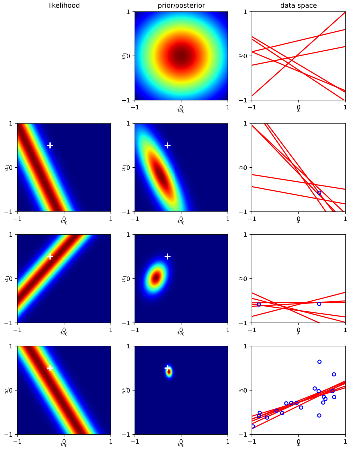
To see sequential learning, take \(y(x,\mathbf{w})=w_0+w_1x\), so the two-dimensional posterior can be drawn. Data come from \(f(x,\mathbf{a})=a_0+a_1x\) with \(a_0=-0.3\), \(a_1=0.5\): inputs \(x_n\sim\mathcal U(-1,1)\), noise standard deviation \(0.2\), so the true \(\beta=(1/0.2)^2=25\), which is also used in the model, and \(\alpha=2.0\). Figure 3.7 shows, row by row: the prior and six lines sampled from it; after one data point, the likelihood of that point (a ridge in \(\mathbf{w}\)-space, the soft constraint that the line pass near it), the posterior (the product with the previous row) and six lines sampled from it, which now pass close to the point; after two points, a compact posterior (two points determine a line); after 20 points, a sharp posterior around the true values (white cross). The key lesson, which Result 3.12 makes exact: the posterior after the second point is the same as the one obtained by combining the original prior with the likelihood of both points at once.
Figure 3.7 (reproduced). Sequential Bayesian learning for \(y=w_0+w_1x\), with \(\alpha=2\), \(\beta=25\) and data from \(a_0=-0.3\), \(a_1=0.5\). Rows: no data, 1, 2 and 20 data points. Left: likelihood of the latest point alone; centre: posterior (prior in the first row), with the true parameters marked by a white cross; right: the data seen so far (blue) and six lines drawn from the posterior. The posterior contracts around the truth as data arrive: in our run the posterior mean and standard deviation of \((w_0,w_1)\) are \((-0.45,-0.20)\) and \((0.33,0.65)\) for \(N=1\), \((-0.55,0.02)\) and \((0.14,0.21)\) for \(N=2\), and \((-0.275,0.418)\) and \((0.045,0.078)\) for \(N=20\). Book: Figure 3.7, p. 155. Code: ch03_linear_regression.py, fig3_7. Download: PDF · SVG
▶ DemoPrior samples (Figure 3.7, first row)Before any data, the prior over \((w_0,w_1)\) is a round Gaussian and the sampled lines fan out in all directions.
▶ DemoAfter one data point (Figure 3.7, second row)The likelihood is a ridge through the weight plane; the sampled lines all pass close to the observed point but their slopes are still uncertain.
▶ DemoAfter 20 pointsThe posterior is concentrated around the generating line; the shrinking of the posterior covariance \(\mathbf{S}_N\) is visible.
3.3.2 Predictive distribution
pp. 156–158 One rarely wants \(\mathbf{w}\) itself, but predictions at new inputs. The predictive distribution averages the likelihood of a new target over the posterior,
The first term of the variance is the noise in the data; the second reflects uncertainty in \(\mathbf{w}\). Always \(\sigma_N^2(\mathbf{x})\ge1/\beta\).
Erratum. The book's cross-reference just before (3.58) to Section 8.1.4 should be to Section 2.3.3.
Proof (two ways)
(i) Constructive. Under the posterior, \(\mathbf{w}\sim\N(\mathbf{m}_N,\mathbf{S}_N)\), and a new target is \(t=\mathbf{w}^\T\bm\phi+\epsilon\) with \(\epsilon\sim\N(0,\beta^{-1})\) independent of \(\mathbf{w}\) (given \(\mathbf{w}\), the new noise is independent of the old). Then \(t\) is a linear function of the jointly Gaussian pair \((\mathbf{w},\epsilon)\), hence Gaussian, with mean \(\bm\phi^\T\mathbf{m}_N\) and variance \(\bm\phi^\T\mathbf{S}_N\bm\phi+\beta^{-1}\) (variances of independent summands add). This is (3.58) and (3.59).
(ii) By the book's route. Write the integrand as \(\N(t\given\bm\phi^\T\mathbf{w},\beta^{-1})\N(\mathbf{w}\given\mathbf{m}_N,\mathbf{S}_N)\). This is a linear-Gaussian model, \(p(\mathbf{w})=\N(\bm\mu,\bm\Lambda^{-1})\), \(p(t\given\mathbf{w})\)\({}=\N(\mathbf{A}\mathbf{w}+\mathbf{b},\mathbf{L}^{-1})\) with \(\mathbf{A}=\bm\phi^\T\), \(\mathbf{b}=0\), \(\mathbf{L}^{-1}=\beta^{-1}\), and the marginal is \(\N(\mathbf{A}\bm\mu+\mathbf{b},\mathbf{L}^{-1}+\mathbf{A}\bm\Lambda^{-1}\mathbf{A}^\T)\) (book (2.115), toolkit), i.e. mean \(\bm\phi^\T\mathbf{m}_N\) and variance \(\beta^{-1}+\bm\phi^\T\mathbf{S}_N\bm\phi\). Since \(\mathbf{S}_N\) is positive definite, \(\bm\phi^\T\mathbf{S}_N\bm\phi\ge0\). ∎
Result 3.14 (the predictive variance shrinks as data arrive) p. 156; Exercise 3.11; Qazaz et al. (1997)
For every input \(\mathbf{x}\), \(\sigma_{N+1}^2(\mathbf{x})\)\({}\le\sigma_N^2(\mathbf{x})\) (3.111); more precisely, adding a point with basis vector \(\bm\phi\) lowers the variance by
\[ \sigma_N^2(\mathbf{x})-\sigma_{N+1}^2(\mathbf{x})=\frac{\beta\,\big(\bm\phi(\mathbf{x})^\T\mathbf{S}_N\bm\phi\big)^2}{1+\beta\bm\phi^\T\mathbf{S}_N\bm\phi}\ \ge0 . \]
Moreover, if \(\lambda_{\min}(\bm\Phi^\T\bm\Phi)\to\infty\) as \(N\to\infty\) (for instance for i.i.d. inputs with \(\E[\bm\phi\bm\phi^\T]\) positive definite, where it grows like \(N\)), then \(\bm\phi(\mathbf{x})^\T\mathbf{S}_N\bm\phi(\mathbf{x})\)\({}\le\|\bm\phi(\mathbf{x})\|^2/(\alpha+\beta\lambda_{\min})\)\({}\to0\) and \(\sigma_N^2(\mathbf{x})\to1/\beta\): in the limit only the noise remains.
Proof
By Result 3.12, \(\mathbf{S}_{N+1}\)\({}=\mathbf{S}_N\)\({}-\dfrac{\beta\mathbf{S}_N\bm\phi\bm\phi^\T\mathbf{S}_N}{1+\beta\bm\phi^\T\mathbf{S}_N\bm\phi}\); this is the identity (3.110), \((\mathbf{M}+\mathbf{v}\mathbf{v}^\T)^{-1}\)\({}=\mathbf{M}^{-1}\)\({}-\dfrac{(\mathbf{M}^{-1}\mathbf{v})(\mathbf{v}^\T\mathbf{M}^{-1})}{1+\mathbf{v}^\T\mathbf{M}^{-1}\mathbf{v}}\), with \(\mathbf{M}=\mathbf{S}_N^{-1}\) and \(\mathbf{v}=\sqrt\beta\bm\phi\). Sandwiching between \(\bm\phi(\mathbf{x})^\T\) and \(\bm\phi(\mathbf{x})\) (call it \(\bm\psi\) to avoid a clash): \(\bm\psi^\T\mathbf{S}_{N+1}\bm\psi\)\({}=\bm\psi^\T\mathbf{S}_N\bm\psi\)\({}-\dfrac{\beta(\bm\psi^\T\mathbf{S}_N\bm\phi)^2}{1+\beta\bm\phi^\T\mathbf{S}_N\bm\phi}\). The subtracted term is a non-negative number over a number \(\ge1\) (as \(\mathbf{S}_N\succ0\)), which is the inequality. For the limit: \(\mathbf{S}_N^{-1}\)\({}=\alpha\mathbf{I}\)\({}+\beta\bm\Phi^\T\bm\Phi\succeq(\alpha+\beta\lambda_{\min})\mathbf{I}\), hence \(\mathbf{S}_N\preceq(\alpha+\beta\lambda_{\min})^{-1}\mathbf{I}\) and \(\bm\phi^\T\mathbf{S}_N\bm\phi\)\({}\le\|\bm\phi\|^2/(\alpha+\beta\lambda_{\min})\). ∎
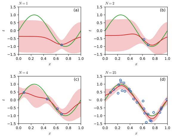
Figure 3.8 (reproduced). The predictive distribution (3.58) for a model of 9 Gaussian basis functions (plus a bias) fitted to the sinusoidal data of Section 1.1 with \(N=1,2,4,25\) points (blue). Red: predictive mean; shaded: one standard deviation each side; green: the generating function \(\sin2\pi x\). The uncertainty is smallest near the data and shrinks as \(N\) grows. Book: Figure 3.8, p. 157. Code: ch03_linear_regression.py, fig3_8. Download: PDF · SVG
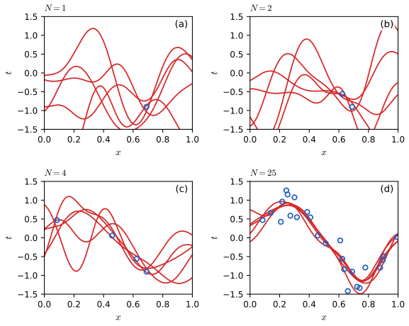
The plots of Figure 3.8 show only the pointwise predictive variance. The joint uncertainty across inputs is visible by drawing weight vectors from the posterior and plotting the functions \(y(x,\mathbf{w})\) (Figure 3.9); it is governed by the covariance (3.63) of Section 3.3.3.
Figure 3.9 (reproduced). Functions \(y(x,\mathbf{w})\) for weight vectors \(\mathbf{w}\) sampled from the posterior of the models in Figure 3.8 (\(N=1,2,4,25\)). Whole curves, rather than pointwise bands, show how the uncertainty at different \(x\) values is coupled: when a sample passes high at one input it tends to pass high at nearby inputs. Book: Figure 3.9, p. 158. Code: ch03_linear_regression.py, fig3_9. Download: PDF · SVG
Filling the gap 3.7: over-confidence away from the basis functions; unknown precision gives a Student t pp. 157–158
The book makes two remarks without proof.
Derivation
Over-confident extrapolation. If the basis functions are localised, say Gaussians (3.4), then for an input \(\mathbf{x}\) far from every centre \(\mu_j\), \(\phi_j(\mathbf{x})\to0\) for all \(j\ge1\) so \(\bm\phi(\mathbf{x})\to(1,0,\dots,0)^\T\) and \(\bm\phi^\T\mathbf{S}_N\bm\phi\)\({}\to(\mathbf{S}_N)_{00}\), which is the posterior variance of the bias alone, small once there is any data. Hence \(\sigma_N^2\)\({}\to\beta^{-1}+(\mathbf{S}_N)_{00}\)\({}\approx\beta^{-1}\): the model claims to know the function as precisely as at the data, where it has no information. This is a failure of the fixed-basis model, not of the Bayesian calculus, and is the reason for Gaussian processes (Section 6.4), whose kernel need not shrink with distance.
Unknown precision. If \(\beta\) is also unknown, with the conjugate prior \(p(\mathbf{w},\beta)\)\({}=\N(\mathbf{w}\given\mathbf{m}_0,\beta^{-1}\mathbf{S}_0)\Gam(\beta\given a_0,b_0)\), the posterior has the same form with parameters \(\mathbf{m}_N,\mathbf{S}_N,a_N,b_N\) (Exercise 3.12) and, integrating out both \(\mathbf{w}\) and \(\beta\), the predictive distribution is a Student t (Exercise 3.13): the heavier tails reflect the extra uncertainty in the noise level. ∎
3.3.3 Equivalent kernel
pp. 159–161 Substituting the posterior mean (3.53) into \(y(\mathbf{x},\mathbf{m}_N)\)\({}=\mathbf{m}_N^\T\bm\phi(\mathbf{x})\) shows that the prediction is a linear combination of the training targets:
\(k\) is the equivalent kernel or smoother matrix, and predictors of this form are linear smoothers. Note that \(k\) depends on the training inputs through \(\mathbf{S}_N\) (but not on the targets).
Result 3.15 (properties of the equivalent kernel) pp. 159–161, (3.63)–(3.65); Exercise 3.14
(a) Covariance. Under the posterior, \(\cov[y(\mathbf{x}),y(\mathbf{x}')]\)\({}=\bm\phi(\mathbf{x})^\T\mathbf{S}_N\bm\phi(\mathbf{x}')\)\({}=\beta^{-1}k(\mathbf{x},\mathbf{x}')\) (3.63); so the kernel says how strongly predictions at \(\mathbf{x}\) and \(\mathbf{x}'\) move together. (b) Inner product. \(k(\mathbf{x},\mathbf{z})\)\({}=\bm\psi(\mathbf{x})^\T\bm\psi(\mathbf{z})\) with \(\bm\psi(\mathbf{x})\)\({}=\beta^{1/2}\mathbf{S}_N^{1/2}\bm\phi(\mathbf{x})\) (3.65); in particular \(k\) is symmetric and positive semi-definite. (c) Summation constraint. If \(\alpha=0\), the basis functions are linearly independent on the training inputs, \(N>M\) and one of the basis functions is the constant, then the weights sum to one for every \(\mathbf{x}\):
For \(\alpha>0\) the sum is no longer exactly one (shrinkage towards the prior mean 0 changes it slightly). The weights can be negative, so predictions are linear combinations, not necessarily convex combinations, of the targets. (d) Smoother matrix. On the training inputs, \(\hat{\mathbf{y}}=\mathbf{K}\mathbf{t}\) with \(\mathbf{K}=\beta\bm\Phi\mathbf{S}_N\bm\Phi^\T\), whose eigenvalues lie in \([0,1)\) (for \(\alpha>0\)) and whose trace is \(\Tr\mathbf{K}\)\({}=\sum_i\frac{\lambda_i}{\lambda_i+\alpha}\)\({}=\gamma\) of (3.91).
Proof
(a) \(y(\mathbf{x})=\bm\phi(\mathbf{x})^\T\mathbf{w}\) with \(\cov\mathbf{w}=\mathbf{S}_N\), so \(\cov[\bm\phi(\mathbf{x})^\T\mathbf{w},\mathbf{w}^\T\bm\phi(\mathbf{x}')]\)\({}=\bm\phi(\mathbf{x})^\T\mathbf{S}_N\bm\phi(\mathbf{x}')\). (b) \(\mathbf{S}_N\) is symmetric positive definite, so it has a symmetric square root \(\mathbf{S}_N^{1/2}\) (from its eigendecomposition) and \(\beta\bm\phi(\mathbf{x})^\T\mathbf{S}_N\bm\phi(\mathbf{z})\)\({}=(\beta^{1/2}\mathbf{S}_N^{1/2}\bm\phi(\mathbf{x}))^\T(\beta^{1/2}\mathbf{S}_N^{1/2}\bm\phi(\mathbf{z}))\); a Gram matrix \(\sum_{ab}c_ac_bk(\mathbf{x}_a,\mathbf{x}_b)\)\({}=\|\sum_ac_a\bm\psi(\mathbf{x}_a)\|^2\)\({}\ge0\).
(c) Direct proof. For \(\alpha=0\), \(\mathbf{S}_N=(\beta\bm\Phi^\T\bm\Phi)^{-1}\), so \(\sum_nk(\mathbf{x},\mathbf{x}_n)\)\({}=\bm\phi(\mathbf{x})^\T(\bm\Phi^\T\bm\Phi)^{-1}\bm\Phi^\T\mathbf{1}\), where \(\mathbf{1}=(1,\dots,1)^\T\). Since one basis function is constant, say \(\phi_0\equiv1\), the vector \(\mathbf{1}\) is the first column of \(\bm\Phi\), so \(\bm\Phi^\T\mathbf{1}\)\({}=\bm\Phi^\T\bm\Phi\mathbf{e}_0\) and the sum equals \(\bm\phi(\mathbf{x})^\T\mathbf{e}_0\)\({}=\phi_0(\mathbf{x})\)\({}=1\). (This is the book's informal argument that least squares fits constant targets exactly.) For \(\alpha>0\), \(\sum_nk\)\({}=\bm\phi^\T(\frac\alpha\beta\mathbf{I}+\bm\Phi^\T\bm\Phi)^{-1}\bm\Phi^\T\bm\Phi\mathbf{e}_0\)\({}=\bm\phi^\T\mathbf{e}_0\)\({}-\frac\alpha\beta\bm\phi^\T(\frac\alpha\beta\mathbf{I}+\bm\Phi^\T\bm\Phi)^{-1}\mathbf{e}_0\), which differs from 1 by a term of order \(\alpha/\beta\), vanishing as \(\alpha\to0\) or as \(N\to\infty\). A fully worked version using orthonormalised basis functions is Exercise 3.14.
(d) On the training inputs \(\mathbf{K}\)\({}=\beta\bm\Phi\mathbf{S}_N\bm\Phi^\T\)\({}=\bm\Phi(\frac\alpha\beta\mathbf{I}+\bm\Phi^\T\bm\Phi)^{-1}\bm\Phi^\T\); with the SVD of Gap 3.2 this is \(\mathbf{U}\operatorname{diag}\big(\frac{s_i^2}{s_i^2+\alpha/\beta}\big)\mathbf{U}^\T\), whose eigenvalues are in \([0,1)\). Its trace, by cyclicity, is \(\Tr[\beta\mathbf{S}_N\bm\Phi^\T\bm\Phi]\)\({}=\Tr[\mathbf{S}_N(\mathbf{S}_N^{-1}-\alpha\mathbf{I})]\)\({}=M-\alpha\Tr\mathbf{S}_N\)\({}=\sum_i\big(1-\frac\alpha{\lambda_i+\alpha}\big)\)\({}=\sum_i\frac{\lambda_i}{\lambda_i+\alpha}\) where \(\lambda_i=\beta d_i\) are the eigenvalues of \(\beta\bm\Phi^\T\bm\Phi\). ∎
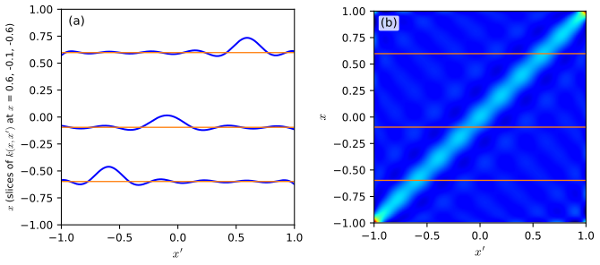
Figure 3.10 (reproduced). The equivalent kernel \(k(x,x')\) of (3.62) for the Gaussian basis functions of Figure 3.1, shown as an image over \((x,x')\) (left) and as three slices, functions of \(x'\) for fixed \(x\) (right); 200 data inputs equally spaced on \([-1,1]\). The kernel is concentrated along the diagonal \(x'\approx x\): the predictive mean at \(x\) is a weighted average of the targets with most weight on nearby inputs. Book: Figure 3.10, p. 159. Code: ch03_linear_regression.py, fig3_10. Download: PDF · SVG
▶ DemoEquivalent kernel (Figure 3.10)Move the reference point \(x\) and watch the weights \(k(x,x_n)\) follow it; they sum to one and can dip slightly below zero.
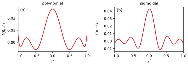
Figure 3.11 (reproduced). Equivalent kernels \(k(x,x')\) for \(x=0\) as a function of \(x'\), for polynomial basis functions (left) and sigmoidal basis functions (right) of Figure 3.1. Even though these basis functions are not local, the equivalent kernel is localised around \(x\). For the Gaussian-basis kernel of Figure 3.10 (\(\alpha=0.005\), \(\beta=11.1\)) our row sums \(\sum_nk(x,x_n)\) are 1.000 at interior \(x\), as (3.64) predicts. Book: Figure 3.11, p. 160. Code: ch03_linear_regression.py, fig3_11. Download: PDF · SVG
This suggests an alternative way to do regression: instead of choosing basis functions (which implicitly fix a kernel), choose a localised kernel directly and predict with \(\sum_nk(\mathbf{x},\mathbf{x}_n)t_n\). That is the programme of kernel methods (Chapter 6) and Gaussian processes (Section 6.4): by (a) and (b), the posterior distribution of the function \(y(\mathbf{x})=\mathbf{w}^\T\bm\phi(\mathbf{x})\) in Bayesian linear regression is itself a Gaussian process, with mean function \(y(\mathbf{x},\mathbf{m}_N)\) and covariance function \(\beta^{-1}k\). Erratum. The book says "effective kernel" once at the start of the paragraph on p. 160; the term is "equivalent kernel".
3.4 Bayesian model comparison
pp. 161–165 Over-fitting is a symptom of maximum likelihood, not of Bayesian inference: if parameters are integrated out instead of point-estimated, models can be compared on the training data alone, with no validation set, and several complexity parameters can be tuned at once (the relevance vector machine of Chapter 7 has one per data point). Suppose we have \(L\) candidate models \(\{\mathcal M_i\}\), each a probability distribution over the observed data \(\mathcal D\) (for curve fitting, over the targets \(\mathbf{t}\) given known inputs). We are uncertain which generated the data, expressed by a prior \(p(\mathcal M_i)\). Given \(\mathcal D\), Bayes' theorem gives
With equal priors the interesting term is the model evidence or marginal likelihood \(p(\mathcal D\given\mathcal M_i)\), the likelihood as a function of the model with the parameters marginalised out. The ratio \(p(\mathcal D\given\mathcal M_i)/p(\mathcal D\given\mathcal M_j)\) is a Bayes factor (Kass and Raftery, 1995). Predictions follow from the sum and product rules as a model average,
a mixture of the individual predictive distributions. If two models are equally probable and one predicts a narrow density near \(t=a\), the other near \(t=b\), the average is bimodal with modes at \(a\) and \(b\), not a single mode at \((a+b)/2\). Model selection is the cheap approximation that keeps only the most probable model. For a model with parameters \(\mathbf{w}\),
which is the probability of generating \(\mathcal D\) from a model whose parameters are drawn at random from the prior; it is also exactly the normaliser in Bayes' theorem for the parameters,
Consider one parameter \(w\) and drop \(\mathcal M_i\) from the notation. If the posterior is sharply peaked at \(w_{\rm MAP}\) with width \(\Delta w_{\rm posterior}\) and the prior is flat of width \(\Delta w_{\rm prior}\), so \(p(w)=1/\Delta w_{\rm prior}\), then approximating the integral by the height times the width of the peak,
The first term is the fit to the data at the best parameter; the second is negative (\(\Delta w_{\rm posterior}<\Delta w_{\rm prior}\)) and is larger in magnitude the more finely the parameter must be tuned. With \(M\) parameters, each with the same ratio,
so the penalty grows linearly with \(M\). Adding parameters raises the first term (better fit) and lowers the second; the maximum evidence is the best compromise.
Figure 3.12 (redrawn). A rough evidence estimate: with a sharply peaked posterior around \(w_{\rm MAP}\) of width \(\Delta w_{\rm posterior}\) and a flat prior of width \(\Delta w_{\rm prior}\), the evidence is the peak likelihood times the Occam factor \(\Delta w_{\rm posterior}/\Delta w_{\rm prior}\). Book: Figure 3.12, p. 163.
Result 3.16 (the Occam factor of a Gaussian linear model; the evidence as accumulated prediction) pp. 162–163, (3.70)–(3.72)
For the Bayesian linear model with prior \(\N(0,\alpha^{-1}\mathbf{I})\), noise precision \(\beta\) and posterior \(\N(\mathbf{m}_N,\mathbf{S}_N)\), the approximation (3.70) is exact, and reads
\[ \ln p(\mathbf{t}\given\alpha,\beta)=\underbrace{\ln p(\mathbf{t}\given\mathbf{m}_N,\beta)}_{\text{fit at the MAP}}\;\underbrace{-\frac\alpha2\mathbf{m}_N^\T\mathbf{m}_N-\frac12\sum_{i=1}^{M}\ln\Big(1+\frac{\lambda_i}\alpha\Big)}_{\text{Occam factor}\ (\le0)}, \]
where \(\lambda_i\) are the eigenvalues of \(\beta\bm\Phi^\T\bm\Phi\). Each factor \(\big(1+\lambda_i/\alpha\big)^{-1/2}\)\({}=\sqrt{\operatorname{var}_{\rm post,i}/\operatorname{var}_{\rm prior,i}}\), the ratio of posterior to prior width along the eigendirection \(\mathbf{u}_i\), is the multi-parameter analogue of \(\Delta w_{\rm posterior}/\Delta w_{\rm prior}\). In addition, for any model, the chain rule gives
\[ \ln p(\mathcal D\given\mathcal M)=\sum_{n=1}^{N}\ln p(t_n\given t_1,\dots,t_{n-1},\mathcal M), \]
so the evidence is the accumulated one-step-ahead predictive score: a model that must learn many parameters spends its early predictions poorly and is charged for that.
Proof
By Bayes' theorem (3.69) rearranged at \(\mathbf{w}=\mathbf{m}_N\), \(p(\mathbf{t}\given\alpha,\beta)\)\({}=p(\mathbf{t}\given\mathbf{m}_N,\beta)\,p(\mathbf{m}_N\given\alpha)/p(\mathbf{m}_N\given\mathbf{t})\). The posterior density at its mean is \(\N(\mathbf{m}_N\given\mathbf{m}_N,\mathbf{S}_N)\)\({}=(2\pi)^{-M/2}|\mathbf{S}_N|^{-1/2}\)\({}=(2\pi)^{-M/2}|\mathbf{A}|^{1/2}\) with \(\mathbf{A}=\mathbf{S}_N^{-1}\), and the prior density is \((\alpha/2\pi)^{M/2}e^{-\alpha\mathbf{m}_N^\T\mathbf{m}_N/2}\). Hence \(\ln p(\mathbf{t}\given\alpha,\beta)\)\({}=\ln p(\mathbf{t}\given\mathbf{m}_N,\beta)\)\({}+\frac M2\ln\alpha\)\({}-\frac\alpha2\mathbf{m}_N^\T\mathbf{m}_N\)\({}-\frac12\ln|\mathbf{A}|\). Since \(\mathbf{A}\)\({}=\alpha\mathbf{I}+\beta\bm\Phi^\T\bm\Phi\) has eigenvalues \(\alpha+\lambda_i\), \(\frac M2\ln\alpha-\frac12\ln|\mathbf{A}|\)\({}=-\frac12\sum_i\ln\frac{\alpha+\lambda_i}\alpha\). The posterior variance along \(\mathbf{u}_i\) is \(1/(\alpha+\lambda_i)\) and the prior variance \(1/\alpha\), whose ratio is \((1+\lambda_i/\alpha)^{-1}\). Substituting \(\ln p(\mathbf{t}\given\mathbf{m}_N,\beta)\)\({}=\frac N2\ln\frac\beta{2\pi}\)\({}-\beta E_D(\mathbf{m}_N)\) reproduces (3.86) of Result 3.18, which verifies the claim. The chain-rule identity is the product rule applied to \(p(t_1,\dots,t_N\given\mathcal M)\), each factor being a predictive distribution of the kind (3.57) (for the linear model, the Gaussian (3.58) with the data so far). ∎
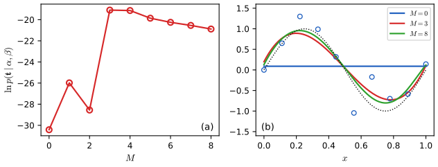
▶ DemoEvidence against model complexity: fewer dataWith fewer data points the evidence prefers a simpler polynomial; with more data it can afford a richer model, because each extra parameter is charged less relative to the improvement in fit.
Why intermediate complexity can win (Figure 3.13)
Put a one-dimensional axis for "the space of possible data sets" and run three models of increasing complexity generatively: pick parameters from the prior, then sample data. A simple model (a first-order polynomial) produces similar data sets every time, so its distribution \(p(\mathcal D\given\mathcal M_1)\) is concentrated in a small region. A complex model (ninth order) produces a great variety, so \(p(\mathcal D\given\mathcal M_3)\) is spread over a large region. Because each distribution integrates to one, the broad one is low everywhere. A data set \(\mathcal D_0\) in the region where the simple model is too rigid but the complex one is too diffuse has the largest evidence under the model of intermediate complexity \(\mathcal M_2\). Complexity is penalised not by counting parameters but by the normalisation of \(p(\mathcal D\given\mathcal M)\). (The book's Figure 3.13 is a schematic and is not reproduced numerically here; Figure 3.14 below is its numerical counterpart.)
Result 3.17 (on average the Bayes factor favours the true model) p. 164, (3.73)
Suppose the data are generated by \(\mathcal M_1\), with distribution \(p(\mathcal D\given\mathcal M_1)\). Then the expected log Bayes factor is a KL divergence and therefore non-negative,
with equality if and only if the two evidence functions are equal almost everywhere. For an individual data set the Bayes factor can favour the wrong model; the statement is about the average. In addition, the plain (not logarithmic) Bayes factor of the wrong model has expectation exactly one: \(\E_{\mathcal M_1}\big[p(\mathcal D\given\mathcal M_2)/p(\mathcal D\given\mathcal M_1)\big]\)\({}=1\) when \(p(\cdot\given\mathcal M_2)\) is supported inside the support of \(p(\cdot\given\mathcal M_1)\).
Proof
The left side of (3.73) is the definition of \(\KL(p_1\|p_2)\) with \(p_i=p(\cdot\given\mathcal M_i)\). Non-negativity: let \(f=-\ln\) (strictly convex). By Jensen's inequality (toolkit, KL), \(\KL(p_1\|p_2)\)\({}=\E_{p_1}[-\ln(p_2/p_1)]\)\({}\ge-\ln\E_{p_1}[p_2/p_1]\)\({}=-\ln\int p_2\,\d\mathcal D\)\({}\ge-\ln1\)\({}=0\), the last inequality because \(\int_{\{p_1>0\}}p_2\le1\); equality in Jensen needs \(p_2/p_1\) constant \(p_1\)-a.e., so \(p_2=p_1\). For the second claim, \(\E_{p_1}[p_2/p_1]=\int_{\{p_1>0\}}p_2=1\) under the support condition. The contrast between the two statements is itself instructive: the Bayes factor \(p_2/p_1\) is 1 on average, yet its logarithm is negative on average (Jensen), so the wrong model usually loses and occasionally wins big. ∎
This relies on the true distribution being among the models considered (the "closed-world" assumption). Two further cautions from the book: the evidence is sensitive to the prior's details (Figure 3.12, e.g. the tails), and it is undefined for an improper prior (an arbitrary scale factor, or, in the limit of a Gaussian prior with infinite variance, the evidence tends to zero as (3.70) shows); one can still compare an evidence ratio of two models first and take the limit afterwards. Hence, in applications, keep an independent test set to assess the final system.
3.5 The evidence approximation
pp. 165–172 A fully Bayesian treatment would also put hyperpriors on \(\alpha\) and \(\beta\) and predict by
One can integrate analytically over \(\mathbf{w}\) or over the hyperparameters, but not over everything. The evidence approximation (also called empirical Bayes, type-2 maximum likelihood or generalised maximum likelihood; Gull, 1989; MacKay, 1992) assumes that \(p(\alpha,\beta\given\mathbf{t})\) is sharply peaked at \(\hat\alpha,\hat\beta\), so that
By Bayes' theorem \(p(\alpha,\beta\given\mathbf{t})\)\({}\propto p(\mathbf{t}\given\alpha,\beta)\,p(\alpha,\beta)\) (3.76), so if the hyperprior is relatively flat, \(\hat\alpha,\hat\beta\) maximise the marginal likelihood \(p(\mathbf{t}\given\alpha,\beta)\), obtained by first integrating out \(\mathbf{w}\). This sets the hyperparameters, and hence the effective regularisation \(\lambda=\alpha/\beta\), from the training data alone. (With Gamma hyperpriors, the integral over \(\alpha,\beta\) gives a Student t over \(\mathbf{w}\); the remaining integral over \(\mathbf{w}\) could then be Laplace-approximated, but its skewed integrand makes that approximation poorer than the evidence procedure (MacKay, 1999).) The maximisation can be done either by differentiating the evidence analytically, as below, or by EM (Section 9.3.4), which reaches the same solution.
3.5.1 Evaluation of the evidence function
pp. 166–168 The marginal likelihood integrates the weights out,
Result 3.18 (the evidence function) pp. 166–167, (3.78)–(3.86); Exercises 3.16–3.19
With \(E(\mathbf{w})\)\({}=\beta E_D(\mathbf{w})+\alpha E_W(\mathbf{w})\)\({}=\frac\beta2\|\mathbf{t}-\bm\Phi\mathbf{w}\|^2\)\({}+\frac\alpha2\mathbf{w}^\T\mathbf{w}\) (3.79),
Completing the square, \(E(\mathbf{w})\)\({}=E(\mathbf{m}_N)\)\({}+\frac12(\mathbf{w}-\mathbf{m}_N)^\T\mathbf{A}(\mathbf{w}-\mathbf{m}_N)\) (3.80) with
where \(\mathbf{A}=\mathbf{S}_N^{-1}\) of (3.54), so \(\mathbf{m}_N\) is the posterior mean. Then \(\int\exp\{-E\}\d\mathbf{w}\)\({}=\exp\{-E(\mathbf{m}_N)\}(2\pi)^{M/2}|\mathbf{A}|^{-1/2}\) (3.85) and
(3.78). From (3.11), (3.12): \(p(\mathbf{t}\given\mathbf{w},\beta)\)\({}=(\beta/2\pi)^{N/2}\exp\{-\beta E_D(\mathbf{w})\}\), and from (3.52): \(p(\mathbf{w}\given\alpha)\)\({}=(\alpha/2\pi)^{M/2}\exp\{-\alpha E_W(\mathbf{w})\}\). Multiply and integrate; the exponents add to \(-E(\mathbf{w})\) (Exercise 3.17).
(3.80)–(3.84). Expand: \(E(\mathbf{w})\)\({}=\frac\beta2\mathbf{t}^\T\mathbf{t}\)\({}-\beta\mathbf{t}^\T\bm\Phi\mathbf{w}\)\({}+\frac12\mathbf{w}^\T(\beta\bm\Phi^\T\bm\Phi+\alpha\mathbf{I})\mathbf{w}\)\({}=\frac\beta2\mathbf{t}^\T\mathbf{t}\)\({}-\beta\mathbf{t}^\T\bm\Phi\mathbf{w}\)\({}+\frac12\mathbf{w}^\T\mathbf{A}\mathbf{w}\). The Hessian is \(\mathbf{A}\) (matrix calculus), positive definite for \(\alpha>0\). Since \(\nabla E\)\({}=\mathbf{A}\mathbf{w}\)\({}-\beta\bm\Phi^\T\mathbf{t}\), the unique minimiser is \(\mathbf{m}_N\)\({}=\beta\mathbf{A}^{-1}\bm\Phi^\T\mathbf{t}\), and a quadratic equals its minimum plus half the Hessian form in the displacement: \(E(\mathbf{w})\)\({}=E(\mathbf{m}_N)\)\({}+\frac12(\mathbf{w}-\mathbf{m}_N)^\T\mathbf{A}(\mathbf{w}-\mathbf{m}_N)\), which is (3.80). To get the value (3.82), evaluate \(E\) at \(\mathbf{m}_N\): this is directly \(\frac\beta2\|\mathbf{t}-\bm\Phi\mathbf{m}_N\|^2\)\({}+\frac\alpha2\mathbf{m}_N^\T\mathbf{m}_N\) by the definition (3.79). Equivalently, using \(\mathbf{A}\mathbf{m}_N=\beta\bm\Phi^\T\mathbf{t}\): \(E(\mathbf{m}_N)\)\({}=\frac\beta2\mathbf{t}^\T\mathbf{t}\)\({}-\beta\mathbf{t}^\T\bm\Phi\mathbf{m}_N\)\({}+\frac12\mathbf{m}_N^\T\mathbf{A}\mathbf{m}_N\)\({}=\frac\beta2\mathbf{t}^\T\mathbf{t}\)\({}-\frac12\mathbf{m}_N^\T\mathbf{A}\mathbf{m}_N\) (Exercise 3.18). That \(\mathbf{m}_N\) equals the mean (3.53) follows from \(\mathbf{A}=\mathbf{S}_N^{-1}\).
(3.85), (3.86). The remaining integral is a Gaussian integral, \(\int\exp\{-\frac12(\mathbf{w}-\mathbf{m}_N)^\T\mathbf{A}(\mathbf{w}-\mathbf{m}_N)\}\d\mathbf{w}\)\({}=(2\pi)^{M/2}|\mathbf{A}|^{-1/2}\), the reciprocal of the normaliser of \(\N(\mathbf{m}_N,\mathbf{A}^{-1})\). Taking logs of (3.78) with this value: \(\frac N2\ln\beta-\frac N2\ln2\pi\)\({}+\frac M2\ln\alpha-\frac M2\ln2\pi\)\({}-E(\mathbf{m}_N)+\frac M2\ln2\pi\)\({}-\frac12\ln|\mathbf{A}|\); the two \(\frac M2\ln2\pi\) terms cancel, giving (3.86). ∎
Filling the gap 3.8: a second derivation of (3.86) by the linear-Gaussian formula p. 166, Exercise 3.16
The book notes that (3.77) can also be done with (2.115). This route gives the evidence in "data space" and is useful when \(NDerivation
In (3.77), \(\mathbf{w}\sim\N(0,\alpha^{-1}\mathbf{I})\) and \(\mathbf{t}\given\mathbf{w}\)\({}\sim\N(\bm\Phi\mathbf{w},\beta^{-1}\mathbf{I})\), so by the linear-Gaussian marginal (toolkit), \(\mathbf{t}\sim\N(0,\mathbf{C})\) with \(\mathbf{C}\)\({}=\beta^{-1}\mathbf{I}_N\)\({}+\alpha^{-1}\bm\Phi\bm\Phi^\T\), i.e. \(\ln p(\mathbf{t}\given\alpha,\beta)\)\({}=-\frac N2\ln2\pi-\frac12\ln|\mathbf{C}|\)\({}-\frac12\mathbf{t}^\T\mathbf{C}^{-1}\mathbf{t}\). Two identities turn this into (3.86). Determinant lemma: \(|\mathbf{C}|\)\({}=\beta^{-N}|\mathbf{I}_N\)\({}+\tfrac\beta\alpha\bm\Phi\bm\Phi^\T|\)\({}=\beta^{-N}|\mathbf{I}_M\)\({}+\tfrac\beta\alpha\bm\Phi^\T\bm\Phi|\)\({}=\beta^{-N}\alpha^{-M}|\mathbf{A}|\) (using \(|\mathbf{I}+\mathbf{U}\mathbf{V}|\)\({}=|\mathbf{I}+\mathbf{V}\mathbf{U}|\)), so \(-\frac12\ln|\mathbf{C}|\)\({}=\frac N2\ln\beta+\frac M2\ln\alpha\)\({}-\frac12\ln|\mathbf{A}|\). Woodbury (toolkit): \(\mathbf{C}^{-1}\)\({}=\beta\mathbf{I}\)\({}-\beta^2\bm\Phi(\alpha\mathbf{I}+\beta\bm\Phi^\T\bm\Phi)^{-1}\bm\Phi^\T\)\({}=\beta\mathbf{I}\)\({}-\beta^2\bm\Phi\mathbf{A}^{-1}\bm\Phi^\T\), so \(\mathbf{t}^\T\mathbf{C}^{-1}\mathbf{t}\)\({}=\beta\mathbf{t}^\T\mathbf{t}\)\({}-\mathbf{m}_N^\T\mathbf{A}\mathbf{m}_N\) because \(\mathbf{m}_N^\T\mathbf{A}\mathbf{m}_N\)\({}=\beta^2\mathbf{t}^\T\bm\Phi\mathbf{A}^{-1}\bm\Phi^\T\mathbf{t}\). By the second form of \(E(\mathbf{m}_N)\) above, \(\frac12\mathbf{t}^\T\mathbf{C}^{-1}\mathbf{t}\)\({}=E(\mathbf{m}_N)\). Together, (3.86). ∎
Figure 3.14 (reproduced). The model log evidence \(\ln p(\mathbf{t}\given\alpha,\beta)\) of (3.86) against the polynomial order \(M\), for the sinusoidal data of Section 1.1 with a prior of the form (1.65), \(\alpha=5\times10^{-3}\). The evidence is highest for \(M=3\): lower orders fit poorly; higher orders improve the fit only marginally (the sine is an odd function, so even powers add nothing, which is why \(M=2\) is below \(M=1\)) and pay a growing complexity penalty. In our run the log evidence is \(-30.42\) at \(M=0\), \(-19.09\) at \(M=3\) (the maximum, with \(M=4\) close behind at \(-19.13\)) and \(-20.88\) at \(M=8\). The test error of Figure 1.5 is roughly constant for \(M=3,\dots,8\), so it cannot discriminate between these orders, whereas the evidence prefers the simplest model that explains the data. Erratum. The book's caption says "model evidence"; the plotted quantity is the log evidence. Book: Figure 3.14, p. 168. Code: ch03_linear_regression.py, fig3_14. Download: PDF · SVG
▶ DemoEvidence against polynomial order (Figure 3.14)Raise the order: the evidence climbs while the model is too simple, peaks at \(M=3\), then falls as the Occam factor of Result 3.16 takes over.
3.5.2 Maximizing the evidence function
pp. 168–170 Define the eigenvalues of the data term by
The eigenvectors of \(\mathbf{A}\)\({}=\alpha\mathbf{I}+\beta\bm\Phi^\T\bm\Phi\) are the same \(\mathbf{u}_i\), with eigenvalues \(\alpha+\lambda_i\), because adding \(\alpha\mathbf{I}\) shifts every eigenvalue by \(\alpha\).
Filling the gap 3.9: the derivative of \(E(\mathbf{m}_N)\) is exact, not an approximation pp. 168–169, text after (3.89); Exercise 3.20
The book differentiates (3.86) with respect to \(\alpha\) and says it "neglects derivatives of \(\mathbf{m}_N^\T\mathbf{m}_N\) with respect to \(\alpha\)". In fact nothing is neglected: the quantity that appears is \(E(\mathbf{m}_N)\), and its total derivative is exactly \(\tfrac12\mathbf{m}_N^\T\mathbf{m}_N\).
Derivation
\(\mathbf{m}_N=\mathbf{m}_N(\alpha,\beta)\) depends on the hyperparameters, so by the chain rule \(\dfrac{\d}{\d\alpha}E(\mathbf{m}_N(\alpha),\alpha)\)\({}=\nabla_{\mathbf{w}}E\big|_{\mathbf{m}_N}^\T\dfrac{\partial\mathbf{m}_N}{\partial\alpha}\)\({}+\dfrac{\partial E}{\partial\alpha}\Big|_{\mathbf{m}_N}\). The first term vanishes because \(\mathbf{m}_N\) minimises \(E\) over \(\mathbf{w}\), so \(\nabla_{\mathbf{w}}E(\mathbf{m}_N)=0\) (the envelope theorem). The second is \(\partial/\partial\alpha\) of \(\frac\beta2\|\mathbf{t}-\bm\Phi\mathbf{w}\|^2\)\({}+\frac\alpha2\mathbf{w}^\T\mathbf{w}\), namely \(\frac12\mathbf{w}^\T\mathbf{w}\), evaluated at \(\mathbf{w}=\mathbf{m}_N\). Likewise \(\dfrac{\d E(\mathbf{m}_N)}{\d\beta}\)\({}=\tfrac12\|\mathbf{t}-\bm\Phi\mathbf{m}_N\|^2\). (Note that \(\mathbf{m}_N^\T\mathbf{m}_N\) does depend on \(\alpha\), but its derivative is not needed.) ∎
Result 3.19 (stationarity conditions for \(\alpha\) and \(\beta\)) pp. 168–170, (3.88)–(3.95); Exercises 3.20–3.22
Let \(\gamma=\sum_i\dfrac{\lambda_i}{\alpha+\lambda_i}\) (3.91). The stationary points of (3.86) satisfy
These are implicit (\(\gamma\) and \(\mathbf{m}_N\) depend on \(\alpha,\beta\)), so they are used as fixed-point iterations: start from \(\alpha,\beta\), compute \(\mathbf{m}_N\) and \(\gamma\), re-estimate. The eigenvalues of \(\bm\Phi^\T\bm\Phi\) can be computed once; \(\lambda_i\) is then \(\beta\) times these. At a joint fixed point \(2E(\mathbf{m}_N)=N\) (Exercise 3.15).
Proof
The \(\alpha\) equation. Differentiate the four \(\alpha\)-dependent terms of (3.86). First, \(\frac{\d}{\d\alpha}\frac M2\ln\alpha\)\({}=\frac M{2\alpha}\). Second, by Gap 3.9, \(-\frac{\d}{\d\alpha}E(\mathbf{m}_N)\)\({}=-\frac12\mathbf{m}_N^\T\mathbf{m}_N\). Third, since \(|\mathbf{A}|=\prod_i(\lambda_i+\alpha)\) (the determinant is the product of the eigenvalues) and \(\lambda_i=\beta d_i\) does not depend on \(\alpha\),
Therefore \(\dfrac{\d\ln p}{\d\alpha}\)\({}=\dfrac M{2\alpha}\)\({}-\dfrac12\mathbf{m}_N^\T\mathbf{m}_N\)\({}-\dfrac12\sum_i\dfrac1{\lambda_i+\alpha}\) (3.89). Multiplying the stationarity condition by \(2\alpha\), \(0\)\({}=M-\alpha\mathbf{m}_N^\T\mathbf{m}_N\)\({}-\alpha\sum_i\frac1{\lambda_i+\alpha}\), i.e. \(\alpha\mathbf{m}_N^\T\mathbf{m}_N\)\({}=M-\alpha\sum_i\frac1{\lambda_i+\alpha}\)\({}=\gamma\) (3.90), where we used that the sum has \(M\) terms to write \(M\)\({}=\sum_i\frac{\lambda_i+\alpha}{\lambda_i+\alpha}\), so \(M-\alpha\sum_i\frac1{\lambda_i+\alpha}\)\({}=\sum_i\frac{\lambda_i}{\lambda_i+\alpha}\)\({}=\gamma\) (3.91). This is (3.92).
The \(\beta\) equation. The eigenvalues are proportional to \(\beta\), so \(\d\lambda_i/\d\beta=\lambda_i/\beta\), and
With \(\frac{\d}{\d\beta}\frac N2\ln\beta\)\({}=\frac N{2\beta}\) and \(\frac{\d E(\mathbf{m}_N)}{\d\beta}\)\({}=\frac12\|\mathbf{t}-\bm\Phi\mathbf{m}_N\|^2\) (Gap 3.9):
Multiplying by \(2\beta\) and solving for \(1/\beta\): \(N-\gamma=\beta\sum_n(\cdot)^2\), which is (3.95).
Consistency check. Substituting (3.92) and (3.95) into (3.82): \(E(\mathbf{m}_N)\)\({}=\frac\beta2\|\mathbf{t}\)\({}-\bm\Phi\mathbf{m}_N\|^2\)\({}+\frac\alpha2\mathbf{m}_N^\T\mathbf{m}_N\)\({}=\frac{N-\gamma}2+\frac\gamma2\)\({}=\frac N2\). ∎
Filling the gap 3.10: the identity \(\frac{\d}{\d\alpha}\ln|\mathbf{A}|\)\({}=\Tr(\mathbf{A}^{-1}\frac{\d\mathbf{A}}{\d\alpha})\) Exercise 3.21, (3.117)
This is the general-purpose form of (3.88) that also covers matrices whose eigenvectors depend on the parameter (e.g. one \(\alpha_j\) per weight, as in Chapter 7).
Derivation
Let \(\mathbf{A}(\alpha)\) be real symmetric positive definite with eigenvalues \(\mu_i(\alpha)\) and orthonormal eigenvectors \(\mathbf{e}_i(\alpha)\). Then \(\ln|\mathbf{A}|=\sum_i\ln\mu_i\) and \(\Tr(\mathbf{A}^{-1}\mathbf{A}')\)\({}=\sum_i\mathbf{e}_i^\T\mathbf{A}^{-1}\mathbf{A}'\mathbf{e}_i\)\({}=\sum_i\mu_i^{-1}\mathbf{e}_i^\T\mathbf{A}'\mathbf{e}_i\) (trace is basis independent; \(\mathbf{A}^{-1}\mathbf{e}_i\)\({}=\mu_i^{-1}\mathbf{e}_i\)). Differentiate \(\mathbf{A}\mathbf{e}_i=\mu_i\mathbf{e}_i\): \(\mathbf{A}'\mathbf{e}_i+\mathbf{A}\mathbf{e}_i'\)\({}=\mu_i'\mathbf{e}_i+\mu_i\mathbf{e}_i'\); left-multiply by \(\mathbf{e}_i^\T\) and use \(\mathbf{e}_i^\T\mathbf{A}=\mu_i\mathbf{e}_i^\T\): \(\mathbf{e}_i^\T\mathbf{A}'\mathbf{e}_i\)\({}+\mu_i\mathbf{e}_i^\T\mathbf{e}_i'\)\({}=\mu_i'+\mu_i\mathbf{e}_i^\T\mathbf{e}_i'\), so \(\mu_i'=\mathbf{e}_i^\T\mathbf{A}'\mathbf{e}_i\). Hence \(\frac{\d}{\d\alpha}\sum_i\ln\mu_i\)\({}=\sum_i\mu_i'/\mu_i\)\({}=\Tr(\mathbf{A}^{-1}\mathbf{A}')\), which is (3.117). Here \(\mathbf{A}'=\mathbf{I}\), so the trace is \(\Tr\mathbf{A}^{-1}=\sum_i(\alpha+\lambda_i)^{-1}\), the same as (3.88). Similarly for \(\beta\), \(\mathbf{A}'=\bm\Phi^\T\bm\Phi\) and \(\Tr(\mathbf{A}^{-1}\bm\Phi^\T\bm\Phi)\)\({}=\beta^{-1}\Tr[\mathbf{A}^{-1}(\mathbf{A}-\alpha\mathbf{I})]\)\({}=\beta^{-1}(M-\alpha\Tr\mathbf{A}^{-1})\)\({}=\gamma/\beta\), which is (3.93). ∎
Figure 3.16 (reproduced). Left: \(\gamma\) (red) and \(2\alpha E_W(\mathbf{m}_N)\)\({}=\alpha\mathbf{m}_N^\T\mathbf{m}_N\) (blue) against \(\ln\alpha\) for the sinusoidal data with 9 Gaussian basis functions plus a bias (\(M=10\)) and \(\beta\) fixed at its true value 11.1; the optimal \(\alpha\) is where the curves cross, which is (3.90). Right: the log evidence (red) against \(\ln\alpha\) peaks at the crossing, and the test error (blue) is smallest close to it. In our run (\(N=25\), \(\beta=1/0.09\)) the two curves cross at \(\ln\alpha=1.2\), exactly where the evidence peaks, and the test error is lowest near \(\ln\alpha=2.5\). Panel (c), which the book does not have, traces the iteration of (3.92) and (3.95) from \(\alpha=\beta=1\): it converges in 8 steps to \(\alpha=3.392\), \(\beta=14.71\), \(\gamma=6.32\), with the log evidence rising from \(-30.06\) to \(-11.58\), the value found by direct maximisation. Book: Figure 3.16, p. 172. Code: ch03_linear_regression.py, fig3_16. Download: PDF · SVG
▶ DemoMaximising the evidence over alphaSlide \(\alpha\): the log evidence has a single peak where \(\gamma=\alpha\mathbf{m}_N^\T\mathbf{m}_N\); iterate (3.92) and watch it climb the curve.
3.5.3 Effective number of parameters
pp. 170–172 Rotate the axes of weight space to the eigenvectors \(\mathbf{u}_i\) of (3.87). Likelihood contours become axis-aligned ellipses, the eigenvalue \(\lambda_i\) is the curvature of the (scaled) log likelihood in direction \(i\) (small curvature = elongated contour), and the prior contours are circles.
Figure 3.15 (reproduced). Contours of the likelihood (red) and the prior (green), in axes rotated to the eigenvectors of the Hessian. For \(\alpha=0\) the posterior mode is \(\mathbf{w}_{\rm ML}\); for \(\alpha>0\) it is \(\mathbf{w}_{\rm MAP}=\mathbf{m}_N\). Along \(w_1\) the eigenvalue \(\lambda_1\) is small against \(\alpha\), so \(\lambda_1/(\lambda_1+\alpha)\approx0\) and the MAP value is near zero; along \(w_2\), \(\lambda_2\) is large against \(\alpha\), the ratio is near one and the MAP value is near its maximum likelihood value. Book: Figure 3.15, p. 170. Code: ch03_linear_regression.py, fig3_15. Download: PDF · SVG
Result 3.20 (\(\gamma\) is the effective number of well-determined parameters) pp. 170–171, (3.91), (3.95)
(a) \(0\le\gamma\le M\), and \(\gamma\) is strictly decreasing in \(\alpha\) from \(\operatorname{rank}\bm\Phi\) (as \(\alpha\to0\)) to \(0\) (as \(\alpha\to\infty\)). (b) In the eigenbasis, the posterior mean is the maximum likelihood estimate shrunk by the factor \(\lambda_i/(\lambda_i+\alpha)\): \(\mathbf{u}_i^\T\mathbf{m}_N\)\({}=\frac{\lambda_i}{\lambda_i+\alpha}\mathbf{u}_i^\T\mathbf{w}_{\rm ML}\) when \(\bm\Phi^\T\bm\Phi\) is invertible. (c) \(\gamma=\sum_i(1-\rho_i)\) where \(\rho_i=\alpha/(\alpha+\lambda_i)\) is the ratio of posterior to prior variance along \(\mathbf{u}_i\): \(\gamma\) counts the directions in which the data have cut the prior uncertainty. (d) \(\gamma=\Tr\mathbf{K}\) is the effective degrees of freedom of the linear smoother (Result 3.15(d)). (e) When \(\alpha\to0\) and \(\bm\Phi\) has full rank, \(\gamma\to M\) and (3.95) becomes the unbiased variance estimate \(\|\mathbf{t}\)\({}-\bm\Phi\mathbf{w}_{\rm ML}\|^2/(N-M)\) of Result 3.2.
Proof
(a) Each ratio \(\lambda_i/(\lambda_i+\alpha)\in[0,1)\) for \(\lambda_i\ge0\), so \(0\le\gamma\le M\); for \(\lambda_i>0\) it decreases strictly in \(\alpha\), from 1 to 0, and for \(\lambda_i=0\) it is identically 0. (b) \(\mathbf{m}_N\)\({}=\beta\mathbf{A}^{-1}\bm\Phi^\T\mathbf{t}\)\({}=\mathbf{A}^{-1}(\beta\bm\Phi^\T\bm\Phi)\mathbf{w}_{\rm ML}\) since \(\bm\Phi^\T\mathbf{t}\)\({}=\bm\Phi^\T\bm\Phi\mathbf{w}_{\rm ML}\); apply \(\mathbf{u}_i^\T\) using \(\mathbf{A}^{-1}\mathbf{u}_i\)\({}=\mathbf{u}_i/(\alpha+\lambda_i)\) and \(\beta\bm\Phi^\T\bm\Phi\mathbf{u}_i\)\({}=\lambda_i\mathbf{u}_i\). So parameters with \(\lambda_i\gg\alpha\) (well determined by the data) keep their ML values, those with \(\lambda_i\ll\alpha\) are set near zero by the prior (Figure 3.15). (c) The posterior covariance \(\mathbf{S}_N=\mathbf{A}^{-1}\) has eigenvalue \(1/(\alpha+\lambda_i)\), the prior \(1/\alpha\). (d) was shown in Result 3.15(d). (e) With \(\alpha\to0\), each \(\lambda_i/(\lambda_i+\alpha)\to1\), and (3.95) has \(N-M\) in the denominator. ∎
Why \(N-\gamma\) in (3.95). Compare (3.95) with the maximum likelihood (3.21): the divisor \(N\) is replaced by \(N-\gamma\). The univariate analogue: the ML variance \(\sigma^2_{\rm ML}\)\({}=\frac1N\sum_n(x_n-\mu_{\rm ML})^2\) (3.96) is biased because \(\mu_{\rm ML}\) has absorbed part of the noise, using up one degree of freedom, and the unbiased estimate divides by \(N-1\) (3.97). In the regression model the mean function has \(M\) parameters, but only \(\gamma\) of them are determined by the data (the other \(M-\gamma\) are held near zero by the prior and absorb little noise), so the correction is by \(\gamma\), not \(M\). Erratum. The first sentence after (3.97) in the book is to be omitted in corrected printings.
Figure 3.17 (reproduced). The 10 parameters \(w_i\) of the Gaussian basis function model (the posterior mean \(\mathbf{m}_N\)) against the effective number of parameters \(\gamma\), as the hyperparameter \(\alpha\) is varied from \(\infty\) (\(\gamma=0\)) to \(0\) (\(\gamma=M\)). Each \(w_i\) is shrunk to zero for small \(\gamma\); the parameters are released one group at a time as \(\gamma\) grows. Book: Figure 3.17, p. 172. Code: ch03_linear_regression.py, fig3_17. Download: PDF · SVG
Result 3.21 (the limit \(N\gg M\)) p. 171, (3.98), (3.99)
If \(N\gg M\) and the basis vectors \(\bm\phi_n\) are not degenerate, then all parameters are well determined, \(\gamma\simeq M\), and the re-estimation equations become
with \(E_W\) and \(E_D\) as in (3.25) and (3.26). These need no eigenvalue computation, so they are a cheap approximation to the full procedure.
Proof
The matrix \(\bm\Phi^\T\bm\Phi=\sum_n\bm\phi_n\bm\phi_n^\T\) is a sum over data points; if the inputs are i.i.d. and \(\E[\bm\phi\bm\phi^\T]\) is positive definite, its eigenvalues are of order \(N\), so \(\lambda_i=\beta d_i\) grows without bound with \(N\) while \(\alpha\) stays fixed. Then \(\lambda_i/(\lambda_i+\alpha)=1-O(\alpha/N)\) for every \(i\), \(\gamma\)\({}=M-\alpha\sum_i(\lambda_i+\alpha)^{-1}\)\({}=M-O(1/N)\)\({}\to M\). Put \(\gamma=M\) in (3.92) and (3.95) and \(N-\gamma\simeq N\) (since \(M\ll N\)): (3.98) and (3.99), where \(2E_W=\mathbf{m}_N^\T\mathbf{m}_N\) and \(2E_D=\|\mathbf{t}-\bm\Phi\mathbf{m}_N\|^2\). ∎
3.6 Limitations of fixed basis functions
pp. 172–173 Models that are linear combinations of fixed nonlinear basis functions have closed-form least squares and a tractable Bayesian treatment, and with suitable basis functions can approximate any reasonable mapping. They also have a basic weakness: the basis functions are chosen before the data are seen, which is a form of the curse of dimensionality (Section 1.4). The number of basis functions must grow quickly, often exponentially, with the input dimension \(D\).
Filling the gap 3.11: how fast the basis grows p. 173
The book asserts the growth without numbers. Two standard counts make it concrete.
Derivation
Polynomials. The number of monomials \(x_1^{k_1}\cdots x_D^{k_D}\) of total degree exactly \(d\) is the number of ways to distribute \(d\) identical units over \(D\) variables, \(\binom{D+d-1}{d}\) (stars and bars); summing over degrees \(0,\dots,d\) gives \(\binom{D+d}{d}\) (hockey-stick identity). For \(d=3\): \(D=10\) gives \(286\) basis functions, \(D=100\) gives \(176\,851\), and for fixed \(d\) the count grows like \(D^d/d!\). Grids of local functions. To cover the cube \([0,1]^D\) with local bumps spaced by \(1/K\) one needs \(K^D\) of them, e.g. \(K=10\) and \(D=10\) gives \(10^{10}\). Either way, a model with as many weights as basis functions cannot be fitted or even stored when \(D\) is moderate. ∎
Two properties of real data help. First, the inputs typically lie near a lower-dimensional nonlinear manifold (strong correlations among inputs; images of handwritten digits in Chapter 12), so local basis functions need only be placed in regions that contain data. This is the idea of radial basis function networks, support vector machines and relevance vector machines (Chapters 6 and 7). Neural networks, with adaptive sigmoidal basis functions, can instead adapt the directions in input space to which the basis functions respond so that they follow the manifold (Chapter 5). Second, the targets may depend on only a few directions within the manifold, which neural networks can also exploit. Together with the over-confident extrapolation noted in Section 3.3.2, these are the reasons the course turns next to classification (Chapter 4) and then to kernels, sparsity and adaptive bases.
Exercises
All 24 exercises of Chapter 3 (Bishop, 2006, pp. 173–177), restated in my own words, with complete solutions (hidden). Stars give the book's difficulty and "www" marks the exercises with official solutions. Many exercises are the derivations of the results above; their solutions then give the argument in full or point to the exact result that contains it.
Exercise 3.1 (★, www). Show that \(\tanh a=2\sigma(2a)-1\) for the logistic sigmoid \(\sigma\) of (3.6), and hence that \(y(x,\mathbf{w})\)\({}=w_0\)\({}+\sum_{j=1}^Mw_j\sigma\big(\frac{x-\mu_j}s\big)\) (3.101) equals \(y(x,\mathbf{u})\)\({}=u_0\)\({}+\sum_{j=1}^Mu_j\tanh\big(\frac{x-\mu_j}{2s}\big)\) (3.102). Find \(\mathbf{u}\) in terms of \(\mathbf{w}\). Erratum: the book's (3.102) lacks the factor 2 in the denominator of the argument of tanh, and its last line should read \(u_0,w_0\) where it says \(u_1,w_1\).
Solution
\(2\sigma(2a)-1\)\({}=\dfrac2{1+e^{-2a}}-1\)\({}=\dfrac{1-e^{-2a}}{1+e^{-2a}}\)\({}=\dfrac{e^a-e^{-a}}{e^a+e^{-a}}\)\({}=\tanh a\) (multiply numerator and denominator by \(e^a\)). Hence \(\sigma(2a)=\tfrac12(1+\tanh a)\). Put \(a_j=\frac{x-\mu_j}{2s}\), so \(\sigma(\frac{x-\mu_j}s)\)\({}=\sigma(2a_j)\)\({}=\frac12+\frac12\tanh a_j\), and
\[ y(x,\mathbf{w})=w_0+\sum_jw_j\Big(\frac12+\frac12\tanh a_j\Big)=\Big(w_0+\frac12\sum_jw_j\Big)+\sum_j\frac{w_j}2\tanh\Big(\frac{x-\mu_j}{2s}\Big). \]
So \(u_j=w_j/2\) for \(j\ge1\) and \(u_0=w_0+\frac12\sum_{j=1}^Mw_j\). The map \(\mathbf{w}\mapsto\mathbf{u}\) is invertible (\(w_j=2u_j\), \(w_0=u_0-\sum_ju_j\)), so the two families represent exactly the same set of functions.
Exercise 3.2 (★★). Show that \(\bm\Phi(\bm\Phi^\T\bm\Phi)^{-1}\bm\Phi^\T\) (3.103) projects any vector onto the space spanned by the columns of \(\bm\Phi\), and use this to show that the least-squares solution (3.15) is the orthogonal projection of \(\mathbf{t}\) onto the subspace \(\mathcal S\) of Figure 3.2.
Solution
This is Result 3.3: \(\mathbf{P}\) is symmetric and idempotent, its range is \(\operatorname{col}(\bm\Phi)\), and \(\mathbf{v}-\mathbf{P}\mathbf{v}\) is orthogonal to every column. Since \(\bm\Phi\mathbf{w}_{\rm ML}\)\({}=\bm\Phi(\bm\Phi^\T\bm\Phi)^{-1}\bm\Phi^\T\mathbf{t}\)\({}=\mathbf{P}\mathbf{t}\), the fitted vector is the orthogonal projection of \(\mathbf{t}\) onto \(\mathcal S\), the nearest point of \(\mathcal S\) to \(\mathbf{t}\).
Exercise 3.3 (★). Each data point has a weight \(r_n>0\) and the error is \(E_D(\mathbf{w})\)\({}=\frac12\sum_nr_n\{t_n\)\({}-\mathbf{w}^\T\bm\phi(\mathbf{x}_n)\}^2\) (3.104). Find the minimiser, and give two interpretations: (i) data-dependent noise variance, (ii) replicated data points.
Solution
With \(\mathbf{R}=\diag(r_1,\dots,r_N)\), \(E_D\)\({}=\frac12(\mathbf{t}-\bm\Phi\mathbf{w})^\T\mathbf{R}(\mathbf{t}-\bm\Phi\mathbf{w})\), with gradient \(-\bm\Phi^\T\mathbf{R}(\mathbf{t}-\bm\Phi\mathbf{w})\). Setting it to zero,
the minimiser since the Hessian \(\bm\Phi^\T\mathbf{R}\bm\Phi\) is positive definite (for independent columns). (i) If \(t_n\)\({}\sim\N(\mathbf{w}^\T\bm\phi_n,(\beta r_n)^{-1})\), i.e. point \(n\) has its own noise precision \(\beta r_n\), the log likelihood is \(\sum_n\frac12\ln(\beta r_n)\)\({}-\beta E_D(\mathbf{w})+\const\), so its maximiser in \(\mathbf{w}\) is \(\mathbf{w}^\star\): precisely measured points (large \(r_n\)) count more. (ii) For integer \(r_n\), the data set in which point \(n\) is repeated \(r_n\) times has plain sum of squares \(\frac12\sum_nr_n(t_n-\mathbf{w}^\T\bm\phi_n)^2\), the same function.
Exercise 3.4 (★, www). For \(y(\mathbf{x},\mathbf{w})=w_0+\sum_{i=1}^Dw_ix_i\) and the sum of squares (3.106), add independent noise \(\epsilon_i\) (mean 0, variance \(\sigma^2\)) to each input. Show that the error averaged over the noise equals the noise-free error plus a weight-decay term that omits \(w_0\).
Solution
With noisy inputs \(\tilde x_{ni}=x_{ni}+\epsilon_{ni}\), the model output is \(\tilde y_n\)\({}=w_0+\sum_iw_i(x_{ni}+\epsilon_{ni})\)\({}=y_n+\sum_iw_i\epsilon_{ni}\). Then
Take expectations over the \(\epsilon\): the middle term has zero mean since \(\E\epsilon_{ni}=0\) and \(y_n,t_n\) are not random; for the last, \(\E[(\sum_iw_i\epsilon_{ni})^2]\)\({}=\sum_{i,j}w_iw_j\E[\epsilon_{ni}\epsilon_{nj}]\)\({}=\sigma^2\sum_iw_i^2\) using \(\E[\epsilon_i\epsilon_j]=\delta_{ij}\sigma^2\). Hence
(The book's solution writes the penalty as \(\frac12\sum_iw_i^2\sigma^2\) per data point, i.e. summed over the \(N\) points gives the factor \(N\) above.) This is the sum of squares for noise-free inputs plus weight decay with \(\lambda=N\sigma^2\), and \(w_0\) is absent because it multiplies no noisy input. Training with input noise is therefore equivalent to Tikhonov regularisation (Bishop, 1995).
Exercise 3.5 (★, www). Using Lagrange multipliers, show that minimising the regularised error (3.29) is equivalent to minimising the sum of squares (3.12) subject to (3.30), and discuss the relation between \(\eta\) and \(\lambda\).
Solution
Write the constraint as \(\frac12(\sum_j|w_j|^q-\eta)\le0\). The Lagrangian is \(L(\mathbf{w},\lambda)\)\({}=E_D(\mathbf{w})\)\({}+\frac\lambda2(\sum_j|w_j|^q-\eta)\), which in its dependence on \(\mathbf{w}\) is (3.29) (plus the constant \(-\lambda\eta/2\)). For fixed \(\lambda\ge0\), minimising \(L\) over \(\mathbf{w}\) is therefore minimising (3.29); complementary slackness fixes \(\eta=\sum_j|w_j^\star(\lambda)|^q\) when \(\lambda>0\). \(\eta(\lambda)\) is non-increasing in \(\lambda\), and in the convex case \(q\ge1\) every binding \(\eta\) corresponds to some \(\lambda\). Full argument, including the monotonicity and the envelope relation \(\lambda/2=-\d E_D^\star/\d\eta\): Result 3.6.
Exercise 3.6 (★, www). For the multivariate model \(p(\mathbf{t}\given\mathbf{W},\bm\Sigma)\)\({}=\N(\mathbf{t}\given\mathbf{W}^\T\bm\phi(\mathbf{x}),\bm\Sigma)\) (3.107, 3.108), show that each column of \(\mathbf{W}_{\rm ML}\) is given by (3.15), independently of \(\bm\Sigma\), and that \(\bm\Sigma_{\rm ML}\)\({}=\frac1N\sum_n(\mathbf{t}_n-\mathbf{W}_{\rm ML}^\T\bm\phi_n)(\mathbf{t}_n-\mathbf{W}_{\rm ML}^\T\bm\phi_n)^\T\) (3.109).
Solution
With residuals \(\mathbf{r}_n=\mathbf{t}_n-\mathbf{W}^\T\bm\phi_n\), \(\ln L\)\({}=-\frac N2\ln|\bm\Sigma|\)\({}-\frac12\sum_n\mathbf{r}_n^\T\bm\Sigma^{-1}\mathbf{r}_n\)\({}+\const\). Since \(\partial\mathbf{r}_n/\partial\mathbf{W}\) gives \(\nabla_{\mathbf{W}}(\frac12\mathbf{r}^\T\bm\Sigma^{-1}\mathbf{r})\)\({}=-\bm\phi\,\mathbf{r}^\T\bm\Sigma^{-1}\) (an \(M\times K\) matrix; matrix calculus), the stationarity condition is \(\sum_n\bm\phi_n\mathbf{r}_n^\T\bm\Sigma^{-1}=0\). Multiply on the right by \(\bm\Sigma\) (invertible): \(\sum_n\bm\phi_n\mathbf{r}_n^\T\)\({}=\bm\Phi^\T(\mathbf{T}-\bm\Phi\mathbf{W})\)\({}=0\), so \(\bm\Phi^\T\bm\Phi\mathbf{W}=\bm\Phi^\T\mathbf{T}\), i.e. \(\mathbf{W}_{\rm ML}\) of (3.34), whose \(k\)th column is (3.15) for \(\mathbf{t}_k\). \(\bm\Sigma\) has dropped out. For \(\bm\Sigma\): with \(\mathbf{W}=\mathbf{W}_{\rm ML}\) and \(\bm\Lambda=\bm\Sigma^{-1}\), the log likelihood is \(\frac N2\ln|\bm\Lambda|\)\({}-\frac12\Tr(\bm\Lambda\sum_n\mathbf{r}_n\mathbf{r}_n^\T)\); its derivative with respect to \(\bm\Lambda\) is \(\frac N2\bm\Lambda^{-1}\)\({}-\frac12\sum_n\mathbf{r}_n\mathbf{r}_n^\T\), zero at \(\bm\Sigma\)\({}=\frac1N\sum_n\mathbf{r}_n\mathbf{r}_n^\T\), which is (3.109) (the standard result for the covariance of a Gaussian, Section 2.3.4). The maximisation is joint, and since \(\mathbf{W}_{\rm ML}\) does not depend on \(\bm\Sigma\) it is the same \(\mathbf{W}_{\rm ML}\) that appears. See also Result 3.7.
Exercise 3.7 (★). By completing the square verify (3.49) for the posterior with \(\mathbf{m}_N\), \(\mathbf{S}_N\) of (3.50), (3.51).
Solution
This is the proof of Result 3.11: the log of likelihood times prior is quadratic in \(\mathbf{w}\) with precision \(\mathbf{S}_0^{-1}+\beta\bm\Phi^\T\bm\Phi\) and linear coefficient \(\mathbf{S}_0^{-1}\mathbf{m}_0\)\({}+\beta\bm\Phi^\T\mathbf{t}\); completing the square identifies the Gaussian with these mean and covariance.
Exercise 3.8 (★★, www). Having observed \(N\) points, treat the posterior (3.49) as the prior for a new point \((\mathbf{x}_{N+1},t_{N+1})\) and show by completing the square that the new posterior is (3.49) with \(\mathbf{S}_{N+1}\), \(\mathbf{m}_{N+1}\).
Solution
Multiplying \(\N(\mathbf{w}\given\mathbf{m}_N,\mathbf{S}_N)\) by \(\exp\{-\frac\beta2(t_{N+1}-\mathbf{w}^\T\bm\phi_{N+1})^2\}\), the exponent (times \(-2\)) is \(\mathbf{w}^\T(\mathbf{S}_N^{-1}+\beta\bm\phi_{N+1}\bm\phi_{N+1}^\T)\mathbf{w}\)\({}-2\mathbf{w}^\T(\mathbf{S}_N^{-1}\mathbf{m}_N+\beta\bm\phi_{N+1}t_{N+1})\)\({}+\const\). Reading off: \(\mathbf{S}_{N+1}^{-1}\)\({}=\mathbf{S}_N^{-1}\)\({}+\beta\bm\phi_{N+1}\bm\phi_{N+1}^\T\) and \(\mathbf{m}_{N+1}\)\({}=\mathbf{S}_{N+1}(\mathbf{S}_N^{-1}\mathbf{m}_N+\beta\bm\phi_{N+1}t_{N+1})\). This is Result 3.12, which also gives the equivalent gain form and shows that the result equals the batch posterior.
Exercise 3.9 (★★). Repeat Exercise 3.8 using the linear-Gaussian result (2.116).
Solution
Take the marginal \(p(\mathbf{w})\)\({}=\N(\mathbf{w}\given\bm\mu,\bm\Lambda^{-1})\) with \(\bm\mu=\mathbf{m}_N\), \(\bm\Lambda=\mathbf{S}_N^{-1}\), and the conditional \(p(t\given\mathbf{w})\)\({}=\N(t\given\mathbf{A}\mathbf{w}+\mathbf{b},\mathbf{L}^{-1})\) with \(\mathbf{A}=\bm\phi_{N+1}^\T\), \(\mathbf{b}=0\), \(\mathbf{L}^{-1}=\beta^{-1}\). Book (2.116) gives the posterior \(\N(\mathbf{w}\given\mathbf{S}\{\mathbf{A}^\T\mathbf{L}(t-\mathbf{b})+\bm\Lambda\bm\mu\},\mathbf{S})\) with \(\mathbf{S}\)\({}=(\bm\Lambda+\mathbf{A}^\T\mathbf{L}\mathbf{A})^{-1}\). Substituting: \(\mathbf{S}\)\({}=(\mathbf{S}_N^{-1}+\beta\bm\phi_{N+1}\bm\phi_{N+1}^\T)^{-1}\)\({}=\mathbf{S}_{N+1}\) and the mean is \(\mathbf{S}_{N+1}(\beta\bm\phi_{N+1}t_{N+1}+\mathbf{S}_N^{-1}\mathbf{m}_N)\)\({}=\mathbf{m}_{N+1}\). (toolkit.)
Exercise 3.10 (★★, www). Using (2.115) to evaluate the integral (3.57), verify the predictive distribution (3.58) with variance (3.59).
Solution
By (3.3), (3.8) and (3.49) the integrand is \(\N(t\given\bm\phi(\mathbf{x})^\T\mathbf{w},\beta^{-1})\,\N(\mathbf{w}\given\mathbf{m}_N,\mathbf{S}_N)\). Matching the first factor to the book's (2.114) \(p(\mathbf{y}\given\mathbf{x})\)\({}=\N(\mathbf{y}\given\mathbf{A}\mathbf{x}+\mathbf{b},\mathbf{L}^{-1})\) with \(\mathbf{A}=\bm\phi(\mathbf{x})^\T\) and the second to (2.113) \(p(\mathbf{x})=\N(\bm\mu,\bm\Lambda^{-1})\), (2.115) gives \(\N(t\given\bm\phi^\T\mathbf{m}_N,\beta^{-1}+\bm\phi^\T\mathbf{S}_N\bm\phi)\). A second, direct proof is given in Result 3.13.
Exercise 3.11 (★★). Use \((\mathbf{M}+\mathbf{v}\mathbf{v}^\T)^{-1}\)\({}=\mathbf{M}^{-1}\)\({}-\frac{(\mathbf{M}^{-1}\mathbf{v})(\mathbf{v}^\T\mathbf{M}^{-1})}{1+\mathbf{v}^\T\mathbf{M}^{-1}\mathbf{v}}\) (3.110) to show \(\sigma_{N+1}^2(\mathbf{x})\)\({}\le\sigma_N^2(\mathbf{x})\) (3.111).
Solution
Take \(\mathbf{M}=\mathbf{S}_N^{-1}\), \(\mathbf{v}=\sqrt\beta\bm\phi_{N+1}\); then \(\mathbf{M}+\mathbf{v}\mathbf{v}^\T\)\({}=\mathbf{S}_{N+1}^{-1}\) and \(\mathbf{S}_{N+1}\)\({}=\mathbf{S}_N\)\({}-\frac{\beta\mathbf{S}_N\bm\phi\bm\phi^\T\mathbf{S}_N}{1+\beta\bm\phi^\T\mathbf{S}_N\bm\phi}\). Hence \(\sigma_N^2(\mathbf{x})\)\({}-\sigma_{N+1}^2(\mathbf{x})\)\({}=\frac{\beta(\bm\phi(\mathbf{x})^\T\mathbf{S}_N\bm\phi_{N+1})^2}{1+\beta\bm\phi_{N+1}^\T\mathbf{S}_N\bm\phi_{N+1}}\)\({}\ge0\), a square over a number at least one (as \(\mathbf{S}_N\) is positive definite). See Result 3.14.
Exercise 3.12 (★★). With both \(\mathbf{w}\) and \(\beta\) unknown, the conjugate prior is \(p(\mathbf{w},\beta)\)\({}=\N(\mathbf{w}\given\mathbf{m}_0,\beta^{-1}\mathbf{S}_0)\Gam(\beta\given a_0,b_0)\) (3.112). Show that the posterior is \(\N(\mathbf{w}\given\mathbf{m}_N,\beta^{-1}\mathbf{S}_N)\Gam(\beta\given a_N,b_N)\) (3.113) and find the parameters.
Solution
Multiply the likelihood \((\beta/2\pi)^{N/2}\exp\{-\frac\beta2\|\mathbf{t}\)\({}-\bm\Phi\mathbf{w}\|^2\}\) by the prior
The exponent in \(\mathbf{w}\) is \(-\frac\beta2\) times a quadratic with precision \(\mathbf{S}_0^{-1}+\bm\Phi^\T\bm\Phi\) (no factor \(\beta\), since \(\beta\) is pulled out) and linear coefficient \(\mathbf{S}_0^{-1}\mathbf{m}_0\)\({}+\bm\Phi^\T\mathbf{t}\). Completing the square (toolkit):
\[ \mathbf{S}_N^{-1}=\mathbf{S}_0^{-1}+\bm\Phi^\T\bm\Phi,\qquad \mathbf{m}_N=\mathbf{S}_N(\mathbf{S}_0^{-1}\mathbf{m}_0+\bm\Phi^\T\mathbf{t}), \]
\[ -\frac\beta2\Big[(\mathbf{w}-\mathbf{m}_N)^\T\mathbf{S}_N^{-1}(\mathbf{w}-\mathbf{m}_N)+\mathbf{t}^\T\mathbf{t}+\mathbf{m}_0^\T\mathbf{S}_0^{-1}\mathbf{m}_0-\mathbf{m}_N^\T\mathbf{S}_N^{-1}\mathbf{m}_N\Big]. \]
The first piece, with the factor \(\beta^{M/2}\) present in the product, is the kernel of \(\N(\mathbf{w}\given\mathbf{m}_N,\beta^{-1}\mathbf{S}_N)\). What is left is a function of \(\beta\) alone,
\[ \beta^{a_0-1+N/2}\exp\Big\{-\beta\Big(b_0+\frac12\big[\mathbf{t}^\T\mathbf{t}+\mathbf{m}_0^\T\mathbf{S}_0^{-1}\mathbf{m}_0-\mathbf{m}_N^\T\mathbf{S}_N^{-1}\mathbf{m}_N\big]\Big)\Big\}, \]
a Gamma kernel with
\[ a_N=a_0+\frac N2,\qquad b_N=b_0+\frac12\Big(\mathbf{m}_0^\T\mathbf{S}_0^{-1}\mathbf{m}_0-\mathbf{m}_N^\T\mathbf{S}_N^{-1}\mathbf{m}_N+\sum_{n=1}^Nt_n^2\Big). \]
An equivalent form is
\[ b_N=b_0+\frac12\Big[\|\mathbf{t}-\bm\Phi\mathbf{m}_N\|^2+(\mathbf{m}_N-\mathbf{m}_0)^\T\mathbf{S}_0^{-1}(\mathbf{m}_N-\mathbf{m}_0)\Big]: \]
the residual at the posterior mean plus the distance from the prior mean, so \(b_N\) accumulates half the "unexplained" squared error. (Both forms agree because the quadratic form in \(\mathbf{w}\) equals its value at \(\mathbf{m}_N\) plus the displacement term.) Hence the posterior has the same form: the prior is conjugate.
Exercise 3.13 (★★). Show that the predictive distribution for the model of Exercise 3.12 is a Student t, \(p(t\given\mathbf{x},\mathbf{t})\)\({}=\St(t\given\mu,\lambda,\nu)\) (3.114), and find \(\mu,\lambda,\nu\).
Solution
Given \(\beta\), the argument of Result 3.13 applies with covariances scaled by \(\beta^{-1}\): \(t=\mathbf{w}^\T\bm\phi+\epsilon\) with \(\mathbf{w}\)\({}\sim\N(\mathbf{m}_N,\beta^{-1}\mathbf{S}_N)\) and \(\epsilon\sim\N(0,\beta^{-1})\), so \(p(t\given\mathbf{x},\mathbf{t},\beta)\)\({}=\N\big(t\given\mathbf{m}_N^\T\bm\phi,\ \beta^{-1}(1+\bm\phi^\T\mathbf{S}_N\bm\phi)\big)\). Now integrate over \(\beta\sim\Gam(a_N,b_N)\): a Gaussian whose precision is \(\beta\Lambda\), with \(\Lambda=1/(1+\bm\phi^\T\mathbf{S}_N\bm\phi)\), mixed over a Gamma-distributed \(\beta\), is a Student t (Section 2.3.7: \(\int\N(x\given\mu,(\beta\Lambda)^{-1})\Gam(\beta\given a,b)\d\beta\)\({}=\St(x\given\mu,\Lambda a/b,2a)\)). Therefore
\[ \mu=\mathbf{m}_N^\T\bm\phi(\mathbf{x}),\qquad \lambda=\frac{a_N}{b_N}\,\frac1{1+\bm\phi(\mathbf{x})^\T\mathbf{S}_N\bm\phi(\mathbf{x})},\qquad \nu=2a_N=2a_0+N. \]
The degrees of freedom grow with \(N\), so the tails become Gaussian as data accumulate; \(b_N/a_N\) plays the role of the noise variance estimate.
Exercise 3.14 (★★). Let the basis functions be linearly independent, \(N>M\), and one of them constant. Take new basis functions \(\psi_j\) spanning the same space and orthonormal on the data, \(\sum_n\psi_j(\mathbf{x}_n)\psi_k(\mathbf{x}_n)\)\({}=I_{jk}\) (3.115). Show that for \(\alpha=0\) the equivalent kernel is \(k(\mathbf{x},\mathbf{x}')\)\({}=\bm\psi(\mathbf{x})^\T\bm\psi(\mathbf{x}')\), and deduce the summation constraint (3.116), \(\sum_nk(\mathbf{x},\mathbf{x}_n)=1\). Erratum: the book's range \(\{\psi_1,\dots,\psi_M\}\) in the exercise should be \(\{\psi_0,\dots,\psi_{M-1}\}\).
Solution
Let \(\bm\psi(\mathbf{x})\)\({}=\mathbf{R}\bm\phi(\mathbf{x})\) for an invertible \(M\times M\) matrix \(\mathbf{R}\) (a change of basis within the same span; for example Gram–Schmidt starting from the constant function, or \(\mathbf{R}=(\bm\Phi^\T\bm\Phi)^{-1/2}\)), and \(\bm\Psi=\bm\Phi\mathbf{R}^\T\). Orthonormality (3.115) says \(\bm\Psi^\T\bm\Psi\)\({}=\mathbf{R}\bm\Phi^\T\bm\Phi\mathbf{R}^\T\)\({}=\mathbf{I}\), so \((\bm\Phi^\T\bm\Phi)^{-1}=\mathbf{R}^\T\mathbf{R}\). For \(\alpha=0\), \(\mathbf{S}_N=(\beta\bm\Phi^\T\bm\Phi)^{-1}\) and
\[ k(\mathbf{x},\mathbf{x}')=\beta\bm\phi^\T(\beta\bm\Phi^\T\bm\Phi)^{-1}\bm\phi'=\bm\phi^\T\mathbf{R}^\T\mathbf{R}\bm\phi'=\bm\psi(\mathbf{x})^\T\bm\psi(\mathbf{x}'). \]
Summation. \(\sum_nk(\mathbf{x},\mathbf{x}_n)\)\({}=\sum_j\psi_j(\mathbf{x})\sum_n\psi_j(\mathbf{x}_n)\). The span contains the constant function, so we may take \(\psi_0\) constant, \(\psi_0\equiv c\); normalisation \(\sum_n\psi_0(\mathbf{x}_n)^2=Nc^2=1\) forces \(c=1/\sqrt N\). (The book's "\(\psi_0=1\)" is not compatible with (3.115) as printed, which requires unit norm; it holds if the normalisation is rescaled. The conclusion is unchanged.) By orthogonality to \(\psi_0\), for each \(j\): \(\sum_n\psi_j(\mathbf{x}_n)\)\({}=\frac1c\sum_n\psi_j(\mathbf{x}_n)\psi_0(\mathbf{x}_n)\)\({}=\delta_{j0}/c\). Hence \(\sum_nk(\mathbf{x},\mathbf{x}_n)\)\({}=\psi_0(\mathbf{x})/c\)\({}=1\). A direct proof is in Result 3.15(c).
Exercise 3.15 (★, www). With \(\alpha\) and \(\beta\) set by the evidence framework, show that \(E(\mathbf{m}_N)\) of (3.82) satisfies \(2E(\mathbf{m}_N)=N\).
Solution
At the stationary values, (3.92) gives \(\alpha\mathbf{m}_N^\T\mathbf{m}_N=\gamma\) and (3.95) gives \(\beta\|\mathbf{t}-\bm\Phi\mathbf{m}_N\|^2\)\({}=N-\gamma\). Then \(2E(\mathbf{m}_N)\)\({}=\beta\|\mathbf{t}-\bm\Phi\mathbf{m}_N\|^2\)\({}+\alpha\mathbf{m}_N^\T\mathbf{m}_N\)\({}=(N-\gamma)+\gamma\)\({}=N\).
Exercise 3.16 (★★). Derive the log evidence (3.86) by using (2.115) to evaluate the integral (3.77) directly.
Solution
See Filling the gap 3.8: (2.115) gives \(\mathbf{t}\)\({}\sim\N(0,\beta^{-1}\mathbf{I}+\alpha^{-1}\bm\Phi\bm\Phi^\T)\); the determinant lemma and the Woodbury identity turn its log density into (3.86).
Exercise 3.17 (★). Show that the evidence can be written in the form (3.78) with \(E(\mathbf{w})\) of (3.79).
Solution
\(p(\mathbf{t}\given\mathbf{w},\beta)\)\({}=(\beta/2\pi)^{N/2}e^{-\beta E_D(\mathbf{w})}\) by (3.10)–(3.12) and \(p(\mathbf{w}\given\alpha)\)\({}=(\alpha/2\pi)^{M/2}e^{-\alpha\mathbf{w}^\T\mathbf{w}/2}\) by (3.52). The product is \((\beta/2\pi)^{N/2}(\alpha/2\pi)^{M/2}\exp\{-\beta E_D\)\({}-\alpha E_W\}\), with \(E_W=\frac12\mathbf{w}^\T\mathbf{w}\); integrating over \(\mathbf{w}\) gives (3.78).
Exercise 3.18 (★★, www). By completing the square over \(\mathbf{w}\), show that \(E(\mathbf{w})\) of (3.79) equals (3.80).
Solution
Expand \(E(\mathbf{w})\)\({}=\frac12[\beta\mathbf{t}^\T\mathbf{t}-2\beta\mathbf{t}^\T\bm\Phi\mathbf{w}+\mathbf{w}^\T\mathbf{A}\mathbf{w}]\) with \(\mathbf{A}\)\({}=\alpha\mathbf{I}+\beta\bm\Phi^\T\bm\Phi\). Since \(\beta\bm\Phi^\T\mathbf{t}=\mathbf{A}\mathbf{m}_N\) (definition (3.84)), \(\beta\mathbf{t}^\T\bm\Phi\mathbf{w}\)\({}=\mathbf{m}_N^\T\mathbf{A}\mathbf{w}\); adding and subtracting \(\mathbf{m}_N^\T\mathbf{A}\mathbf{m}_N\):
\[ E(\mathbf{w})=\tfrac12\beta\mathbf{t}^\T\mathbf{t}-\tfrac12\mathbf{m}_N^\T\mathbf{A}\mathbf{m}_N+\tfrac12(\mathbf{w}-\mathbf{m}_N)^\T\mathbf{A}(\mathbf{w}-\mathbf{m}_N). \]
The first two terms equal \(\frac\beta2\|\mathbf{t}-\bm\Phi\mathbf{m}_N\|^2\)\({}+\frac\alpha2\mathbf{m}_N^\T\mathbf{m}_N\)\({}=E(\mathbf{m}_N)\): expand \(\frac\beta2(\mathbf{t}-\bm\Phi\mathbf{m}_N)^\T(\mathbf{t}-\bm\Phi\mathbf{m}_N)\)\({}+\frac\alpha2\mathbf{m}_N^\T\mathbf{m}_N\)\({}=\frac\beta2\mathbf{t}^\T\mathbf{t}\)\({}-\beta\mathbf{t}^\T\bm\Phi\mathbf{m}_N\)\({}+\frac12\mathbf{m}_N^\T\mathbf{A}\mathbf{m}_N\), and \(\beta\mathbf{t}^\T\bm\Phi\mathbf{m}_N\)\({}=\mathbf{m}_N^\T\mathbf{A}\mathbf{m}_N\), giving \(\frac\beta2\mathbf{t}^\T\mathbf{t}\)\({}-\frac12\mathbf{m}_N^\T\mathbf{A}\mathbf{m}_N\). So (3.80) and (3.82). See Result 3.18.
Exercise 3.19 (★★). Show that integrating over \(\mathbf{w}\) gives (3.85), hence the log marginal likelihood (3.86).
Solution
By (3.80),
\[ \int e^{-E(\mathbf{w})}\d\mathbf{w}=e^{-E(\mathbf{m}_N)}\int\exp\Big\{-\frac12(\mathbf{w}-\mathbf{m}_N)^\T\mathbf{A}(\mathbf{w}-\mathbf{m}_N)\Big\}\d\mathbf{w}, \]
and the last integral is the reciprocal of the normalisation constant \((2\pi)^{-M/2}|\mathbf{A}|^{1/2}\) of \(\N(\mathbf{m}_N,\mathbf{A}^{-1})\), i.e. \((2\pi)^{M/2}|\mathbf{A}|^{-1/2}\): (3.85). Insert in (3.78) and take logs: \(\frac N2\ln\frac\beta{2\pi}\)\({}+\frac M2\ln\frac\alpha{2\pi}-E(\mathbf{m}_N)\)\({}+\frac M2\ln2\pi-\frac12\ln|\mathbf{A}|\), which is (3.86).
Exercise 3.20 (★★, www). Verify all steps leading from the maximisation of (3.86) with respect to \(\alpha\) to the re-estimation equation (3.92). Erratum: the book's wording "Starting from (3.86) verify ..." should read "Verify ...".
Solution
Only the first, third and fourth terms of (3.86) depend on \(\alpha\) (for fixed \(\beta\)). Eigenvalues of \(\mathbf{A}\) are \(\alpha+\lambda_i\) (the eigenvectors \(\mathbf{u}_i\) of \(\beta\bm\Phi^\T\bm\Phi\) are orthonormal and \(\alpha\mathbf{I}\) shifts them), giving (3.88). The derivative of \(E(\mathbf{m}_N)\) is exactly \(\frac12\mathbf{m}_N^\T\mathbf{m}_N\) (Gap 3.9; this justifies the book's "neglected" derivative). Combining gives (3.89), and multiplying by \(2\alpha\) and using \(M\)\({}=\sum_i\frac{\alpha+\lambda_i}{\alpha+\lambda_i}\) gives (3.90), (3.91), (3.92). Every step is written out in Result 3.19.
Exercise 3.21 (★★). Prove \(\frac{\d}{\d\alpha}\ln|\mathbf{A}|\)\({}=\Tr(\mathbf{A}^{-1}\frac{\d\mathbf{A}}{\d\alpha})\) (3.117) using the eigenvalue expansion of a real symmetric matrix, and use it to derive (3.92) from (3.86).
Solution
The proof is in Filling the gap 3.10 (differentiate \(\mathbf{A}\mathbf{e}_i=\mu_i\mathbf{e}_i\), obtain \(\mu_i'=\mathbf{e}_i^\T\mathbf{A}'\mathbf{e}_i\), and sum \(\mu_i'/\mu_i\)). With \(\mathbf{A}'=\mathbf{I}\), \(\Tr\mathbf{A}^{-1}=\sum_i(\alpha+\lambda_i)^{-1}\) and (3.89) follows as before; the rest is Result 3.19.
Exercise 3.22 (★★). Verify all steps leading from the maximisation of (3.86) with respect to \(\beta\) to (3.95).
Solution
The \(\beta\)-dependent terms of (3.86) are \(\frac N2\ln\beta\), \(-E(\mathbf{m}_N)\) and \(-\frac12\ln|\mathbf{A}|\). Their derivatives are \(\frac N{2\beta}\), \(-\frac12\|\mathbf{t}-\bm\Phi\mathbf{m}_N\|^2\) (envelope theorem, Gap 3.9) and \(-\frac\gamma{2\beta}\) (since \(\d\lambda_i/\d\beta=\lambda_i/\beta\), (3.93)). Setting the sum to zero is (3.94); rearranged it is (3.95). See Result 3.19.
Exercise 3.23 (★★, www). For the model of Exercise 3.12, show that the evidence is
\[ p(\mathbf{t})=\frac1{(2\pi)^{N/2}}\frac{b_0^{a_0}}{b_N^{a_N}}\frac{\Gamma(a_N)}{\Gamma(a_0)}\frac{|\mathbf{S}_N|^{1/2}}{|\mathbf{S}_0|^{1/2}} \tag{3.118} \]
by first marginalising over \(\mathbf{w}\) and then over \(\beta\).
Solution
Use the notation of Exercise 3.12 and write \(2(b_N-b_0)\)\({}=\mathbf{t}^\T\mathbf{t}\)\({}+\mathbf{m}_0^\T\mathbf{S}_0^{-1}\mathbf{m}_0\)\({}-\mathbf{m}_N^\T\mathbf{S}_N^{-1}\mathbf{m}_N\). The integrand over \(\mathbf{w}\) is
\[ \Big(\frac\beta{2\pi}\Big)^{(N+M)/2}|\mathbf{S}_0|^{-1/2}\exp\Big\{-\frac\beta2\big[(\mathbf{w}-\mathbf{m}_N)^\T\mathbf{S}_N^{-1}(\mathbf{w}-\mathbf{m}_N)+2(b_N-b_0)\big]\Big\}. \]
The Gaussian integral over \(\mathbf{w}\) is \((2\pi/\beta)^{M/2}|\mathbf{S}_N|^{1/2}\), leaving \((\beta/2\pi)^{N/2}|\mathbf{S}_N|^{1/2}|\mathbf{S}_0|^{-1/2}e^{-\beta(b_N-b_0)}\). Multiply by the Gamma prior \(\frac{b_0^{a_0}}{\Gamma(a_0)}\beta^{a_0-1}e^{-b_0\beta}\) and integrate over \(\beta\): the exponent combines to \(e^{-b_N\beta}\) and the power of \(\beta\) is \(\beta^{a_0+N/2-1}=\beta^{a_N-1}\), with \(\int_0^\infty\beta^{a_N-1}e^{-b_N\beta}\d\beta\)\({}=\Gamma(a_N)/b_N^{a_N}\). Collecting constants gives (3.118).
Exercise 3.24 (★★). Repeat Exercise 3.23 using Bayes' theorem in the form \(p(\mathbf{t})\)\({}=p(\mathbf{t}\given\mathbf{w},\beta)p(\mathbf{w},\beta)/p(\mathbf{w},\beta\given\mathbf{t})\) (3.119).
Solution
The identity holds for every \((\mathbf{w},\beta)\); substitute the three normalised densities. Powers of \(\beta\): the numerator has \(\beta^{N/2}\) (likelihood), \(\beta^{M/2}\) (Gaussian prior), \(\beta^{a_0-1}\) (Gamma prior); the denominator has \(\beta^{M/2}\) (Gaussian posterior) and \(\beta^{a_N-1}\) (Gamma posterior). Their ratio is \(\beta^{N/2+a_0-a_N}=\beta^0\). Powers of \(2\pi\): \((2\pi)^{-N/2-M/2}\) over \((2\pi)^{-M/2}\) gives \((2\pi)^{-N/2}\). Determinants and Gamma constants: \(\frac{|\mathbf{S}_0|^{-1/2}}{|\mathbf{S}_N|^{-1/2}}\cdot\frac{b_0^{a_0}/\Gamma(a_0)}{b_N^{a_N}/\Gamma(a_N)}\). The exponents: the numerator has (Exercise 3.12)
\[ -\frac\beta2\Big[\|\mathbf{t}-\bm\Phi\mathbf{w}\|^2+(\mathbf{w}-\mathbf{m}_0)^\T\mathbf{S}_0^{-1}(\mathbf{w}-\mathbf{m}_0)\Big]-b_0\beta=-\frac\beta2\Big[(\mathbf{w}-\mathbf{m}_N)^\T\mathbf{S}_N^{-1}(\mathbf{w}-\mathbf{m}_N)+2(b_N-b_0)\Big]-b_0\beta, \]
the denominator \(-\frac\beta2(\mathbf{w}-\mathbf{m}_N)^\T\mathbf{S}_N^{-1}(\mathbf{w}-\mathbf{m}_N)\)\({}-b_N\beta\). The \(\mathbf{w}\)-dependence cancels and so does the rest: \(-\beta(b_N-b_0)-b_0\beta+b_N\beta=0\). What remains is (3.118), as it must, because the left side does not depend on \((\mathbf{w},\beta)\).
Demonstrations for this chapter
Each demonstration runs in the browser, with seeded random numbers so that a class sees the same pictures, and links back to these notes. The ▶ Demo boxes above open them already set to the case under discussion.
A linear model with Gaussian basis functions: samples from the prior and posterior, the predictive mean and band, and the equivalent kernel. Presets: 1 prior samples (Fig. 3.7); 2 after one data point (Fig. 3.7); 3 after 20 points; 4 predictive distribution with its band (Fig. 3.8); 5 samples from the posterior (Fig. 3.9); 6 equivalent kernel (Fig. 3.10).
100 data sets, the fitted curves and their average, and the three terms against \(\ln\lambda\). Presets: 1 large \(\lambda\), high bias (Fig. 3.5); 2 moderate \(\lambda\) (Fig. 3.5); 3 small \(\lambda\), high variance (Fig. 3.5); 4 bias squared, variance and test error against \(\ln\lambda\) (Fig. 3.6).
The marginal likelihood against polynomial order, the evidence over \(\alpha\) and \(\beta\), and the effective number of parameters \(\gamma\). Presets: 1 evidence against polynomial order (Fig. 3.14); 2 maximising the evidence over \(\alpha\); 3 the effective number of parameters \(\gamma\) (Section 3.5.3); 4 evidence against complexity with fewer data; 5 eigenvalues and well-determined parameters (Fig. 3.15).
The Python code that produces every figure of this page, and checks the chapter's identities numerically, is code/ch03_linear_regression.py (see the code index).
References
Bishop, C. M. (2006). Pattern Recognition and Machine Learning. Springer, New York. Chapter 3, pp. 137–177 (and the official errata). doi:10.1007/978-0-387-45528-0.
Bishop, C. M. (1995). Training with noise is equivalent to Tikhonov regularization. Neural Computation, 7(1), 108–116. doi:10.1162/neco.1995.7.1.108.
Geman, S., Bienenstock, E. and Doursat, R. (1992). Neural networks and the bias/variance dilemma. Neural Computation, 4(1), 1–58. doi:10.1162/neco.1992.4.1.1.
Gull, S. F. (1989). Developments in maximum entropy data analysis. In J. Skilling (ed.), Maximum Entropy and Bayesian Methods, 53–71. Kluwer, Dordrecht.
Hoerl, A. E. and Kennard, R. W. (1970). Ridge regression: biased estimation for nonorthogonal problems. Technometrics, 12(1), 55–67. doi:10.1080/00401706.1970.10488634.
Kass, R. E. and Raftery, A. E. (1995). Bayes factors. Journal of the American Statistical Association, 90(430), 773–795. doi:10.1080/01621459.1995.10476572.
MacKay, D. J. C. (1999). Comparison of approximate methods for handling hyperparameters. Neural Computation, 11(5), 1035–1068. doi:10.1162/089976699300016331.
Penrose, R. (1955). A generalized inverse for matrices. Mathematical Proceedings of the Cambridge Philosophical Society, 51(3), 406–413. doi:10.1017/S0305004100030401.
Qazaz, C. S., Williams, C. K. I. and Bishop, C. M. (1997). An upper bound on the Bayesian error bars for generalized linear regression. In S. W. Ellacott, J. C. Mason and I. J. Anderson (eds), Mathematics of Neural Networks: Models, Algorithms and Applications, 295–299. Kluwer. doi:10.1007/978-1-4615-6099-9_51.
Robbins, H. and Monro, S. (1951). A stochastic approximation method. The Annals of Mathematical Statistics, 22(3), 400–407. doi:10.1214/aoms/1177729586.
Sherman, J. and Morrison, W. J. (1950). Adjustment of an inverse matrix corresponding to a change in one element of a given matrix. The Annals of Mathematical Statistics, 21(1), 124–127. doi:10.1214/aoms/1177729893.
Tibshirani, R. (1996). Regression shrinkage and selection via the lasso. Journal of the Royal Statistical Society: Series B, 58(1), 267–288. doi:10.1111/j.2517-6161.1996.tb02080.x.
DOIs were checked against Crossref. The numerical statements made in the text (the evidence formula against the direct Gaussian marginal, the exactness of the envelope-theorem derivatives, the fixed point with \(2E(\mathbf{m}_N)=N\), the optimal ridge parameter averaged over the prior, the evidence (3.118) against numerical integration over \(\beta\), the summation constraint of the equivalent kernel) come from short Python computations written for these notes; the figures come from the course code.