Linear and Logistic Regression
Regression studies how a response \(Y\) depends on covariates \(X\) through the regression function \(r(x)=\E(Y\given X=x)\). This chapter of the book takes the parametric route: \(r\) is linear in its parameters, estimated by least squares (which is maximum likelihood under Normal errors), and for a binary response the log-odds are linear and the likelihood is maximised by reweighted least squares. The book states most results without proof. These notes prove them all: the least squares formulas and the unbiasedness of \(\hs^2\), the sampling distribution of \(\hb\) and the conditions behind "under appropriate conditions", the prediction interval (and why it needs Normal errors when the confidence interval does not), the optimism of the training error, the equivalence of AIC and Mallows' \(C_p\), the leave-one-out shortcut, the Laplace argument for BIC, the consistency of the Zheng-Loh method, the existence of the logistic MLE and why Newton's method is reweighted least squares, and Akaike's bias correction. The book's data sets are reanalysed throughout, and one of its numerical examples (the Palm Beach prediction interval) is corrected.
Ch. 1 Probability Ch. 2 Random variables Ch. 3 Expectation Ch. 4 Inequalities Ch. 5 Convergence Ch. 6 Models and inference Ch. 7 Estimating the CDF Ch. 8 Bootstrap Ch. 9 Parametric inference Ch. 10 Hypothesis testing Ch. 11 Bayesian inference Ch. 12 Decision theory Ch. 13 Regression Ch. 14 Multivariate models Ch. 15 Independence Ch. 16 Causal inference Ch. 17 Directed graphs Ch. 18 Undirected graphs Ch. 19 Log-linear models Ch. 20 Curve estimation Ch. 21 Orthogonal functions Ch. 22 Classification Ch. 23 Stochastic processes Ch. 24 Simulation
How to read these notes
They follow the book. Sections carry the book's numbers (13.1 to 13.10) and every displayed equation that appears in the book carries the book's own equation number, e.g. \((13.20)\). Numbered items keep the book's numbers (Definition 13.1, Theorem 13.8, Example 13.17); results the book states without a number, and the new results needed to fill its gaps, are lettered (Theorem 13.A, Algorithm 13.B, ...). Equations without a number are steps that the book skips.
Filling the gaps. Wherever the book says "it can be shown", quotes a result without proof, or leaves an argument implicit, an orange Filling the gap box gives the full argument. Proofs and derivations start hidden: open one with its bar, or use the button below.
Figures and demonstrations. The three figures of the chapter are reproduced (Figures 13.1 to 13.3) on the book's data, and six supplementary figures (13.S1 to 13.S6) illustrate gaps filled in the notes and the computational exercises; all are computed by the Python code. The ▶ Demo boxes open an interactive demonstration already set to the case being discussed.
Main reference
L. Wasserman, All of Statistics: A Concise Course in Statistical Inference, Springer (2004), Chapter 13, pages 209–229 (book website: www.stat.cmu.edu/~larry/all-of-statistics). Section, equation, example and exercise numbers below refer to this book. Further reading is listed in the references.
The explanations, derivations, figures and code are my own; equations are cited by their numbers in the book.
Companion courses
Linear and logistic regression are central to four companion courses on this site. The overlapping material is:
- Applied Statistical Learning in R and Python: Section 3.1 (simple regression: the least squares estimates in Filling the gap 3.1, their standard errors in 3.2, the exact \(t\) interval in 3.3, multiple regression in 3.5 and the confidence and prediction intervals in 3.8) with its regression bands demo; logistic regression in Section 4.3 (Result 4.1, Algorithm 4.1); and subset selection with \(C_p\), AIC and BIC in Section 6.1 (Results 6.2 and 6.3) with its subset selection demo.
- Statistical Learning: Theory and Methods: the linear model in matrix form in Section 3.2 (Results 3.1 to 3.4, the Gauss-Markov theorem in Result 3.6, subset selection in Section 3.3); logistic regression on the same heart disease data in Section 4.4 (Result 4.8) with its IRLS demo; the optimism of the training error, AIC, BIC and cross-validation in Sections 7.4 to 7.10 (Result 7.6, Filling the gap 7.3, Results 7.9, 7.10 and 7.13) with its optimism and Cp demo.
- Foundations of Deep Learning, Section 4.1: maximum likelihood and least squares (Results 4.2 and 4.4), the geometry of least squares (Result 4.5) and the regression function as the optimal predictor (Result 4.9).
- Bayesian and Probabilistic Machine Learning: least squares as maximum likelihood in Result 3.1 and its geometry in Result 3.3; iteratively reweighted least squares in Section 4.3.3 (Algorithm 4.2).
Those courses use regression to predict; this chapter asks the inferential questions: what are the sampling distributions, under which conditions do the Normal approximations hold, and what does each model selection score estimate. Where a proof there is identical, these notes give the statement and a short argument and link to it. New here: the conditions behind Theorem 13.9 (Filling the gap 13.5), why the prediction interval is not rescued by the central limit theorem (13.6), the exact relation between R's AIC and \(C_p\) (13.9), the consistency of the Zheng-Loh method (13.12), the existence of the logistic MLE and the bounded-curvature algorithm (13.13), Akaike's bias calculation (13.15), and the corrected Palm Beach interval (Notes on the book).
The chapter at a glance
- 13.1 The regression function (13.1) is the best predictor (Filling the gap 13.1); the simple linear model (Definition 13.1) is fitted by least squares (Theorem 13.4).
- 13.2 Under Normal errors least squares is maximum likelihood (Theorem 13.7).
- 13.3 The least squares estimates are unbiased with covariance (13.11) (Theorem 13.8), consistent and asymptotically Normal (Theorem 13.9) under conditions made explicit in Filling the gap 13.5.
- 13.4 A prediction interval must add the noise variance (Theorem 13.11), and is valid only for Normal-like errors (13.6).
- 13.5 Multiple regression in matrix form (Theorem 13.13).
- 13.6 The training error is too small by \(2\sum\Cov(\hY_i,Y_i)\) (Theorem 13.15); \(C_p\), AIC, BIC and cross-validation correct for it; greedy searches and the Zheng-Loh method.
- 13.7 Logistic regression (13.32)–(13.35), fitted by reweighted least squares (Algorithm 13.B), with standard errors from the Fisher information.
- 13.9 AIC is an approximately unbiased estimate of the expected log-likelihood of the fitted model (Theorem 13.18).
Notation. Data \((X_1,Y_1),\dots,(X_n,Y_n)\); \(\bX\), \(\bY\) are sample means and \(\Sxx=\sum_i(X_i-\bX)^2=ns_X^2\). Hats denote estimates: \(\hb\), \(\hs\), fitted values \(\hY_i\), residuals \(\he_i=Y_i-\hY_i\), \(\RSS=\sum_i\he_i^2\). In Sections 13.5–13.6, \(X\) is the \(n\times k\) design matrix with rows \(x_i^\T\), \(H=X(X^\T X)^{-1}X^\T\) the hat matrix (the book's \(U\)) with diagonal \(h_{ii}\), and \(\tr\) the trace. Unless said otherwise, moments are conditional on the covariates, \(\Xn=(X_1,\dots,X_n)\); \(z_{\alpha/2}\) is the upper \(\alpha/2\) quantile of \(\N(0,1)\), \(\Phi\) its cdf.
Prerequisites. Conditional expectation and the rule of iterated expectations (Chapter 3), Slutsky's theorem and the central limit theorem (Theorem 5.5, Theorem 5.8), maximum likelihood and its asymptotic normality (Theorem 9.18, 9.27), Newton's method (Chapter 9), the Wald and likelihood ratio tests (Definition 10.3, Theorem 10.22). See the course home.
p. 209 A response \(Y\) and a covariate (predictor, feature) \(X\) are observed together, \((Y_1,X_1),\dots,(Y_n,X_n)\sim F_{X,Y}\). The relationship is summarised by the regression function
\[ r(x)=\E(Y\given X=x)=\int y\,f(y\given x)\,\d y. \tag{13.1} \]This chapter assumes that \(r\) is linear; Chapters 20 and 21 of the book drop that assumption. The word "regression" goes back to Galton (1886), who found that sons of very tall or very short fathers tend to be closer to the average height: they "regress towards the mean".
Filling the gap 13.1: why the regression function is the object of interest p. 209
Assume \(\E Y^2<\infty\). Among all functions \(g\) with \(\E g(X)^2<\infty\), the regression function minimises the mean squared prediction error:
\[ \E\{Y-g(X)\}^2=\E\{Y-r(X)\}^2+\E\{r(X)-g(X)\}^2\ \ge\ \E\{Y-r(X)\}^2 . \]Consequently \(\epsilon=Y-r(X)\) always satisfies \(\E(\epsilon\given X)=0\): the linear model below assumes nothing about the errors' mean beyond linearity of \(r\). Its real assumptions are that \(r\) is linear and, in (13.2), that \(\V(\epsilon\given X)\) does not depend on \(X\).
Proof
Add and subtract \(r(X)\):
\[ \E\{Y-g(X)\}^2=\E\{Y-r(X)\}^2+\E\{r(X)-g(X)\}^2+2\E[\{Y-r(X)\}\{r(X)-g(X)\}]. \] By iterated expectations (Result 3.11) the cross term is \(2\E[\{r(X)-g(X)\}\E\{Y-r(X)\given X\}]\)
The same argument is Result 4.9 of Foundations of Deep Learning.
13.1 Simple Linear Regression
pp. 209–210 With a single covariate and a linear regression function, \(r(x)=\beta_0+\beta_1x\), and the further simplification that the conditional variance does not depend on \(x\), we get the simple linear regression model.
Definition 13.1 (the simple linear regression model) p. 210
\[ Y_i=\beta_0+\beta_1X_i+\epsilon_i, \tag{13.2} \]where \(\E(\epsilon_i\given X_i)=0\) and \(\V(\epsilon_i\given X_i)=\sigma^2\). The unknown parameters are the intercept \(\beta_0\), the slope \(\beta_1\) and the variance \(\sigma^2\). Throughout, the pairs \((X_i,Y_i)\) are independent, so that given \(\Xn\) the errors are independent with mean 0 and variance \(\sigma^2\).
Example 13.2. p. 210 Figure 13.1 plots the log surface temperature (\(Y\)) of stars against their log light intensity (\(X\)). The stars are those of the cluster CYG OB1 (Humphreys 1978, as tabulated by Rousseeuw and Leroy 1987), 47 in all; the book's plot shows log temperatures between 4.0 and 4.6 only, and indeed its line is reproduced exactly when the five stars with log temperature below 4.0 (the four red giants and one other star) are left out, leaving \(n=42\).
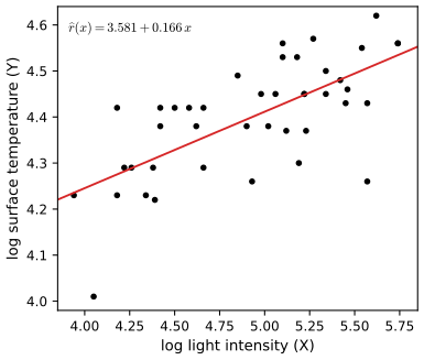
fig_13_1. Download: PDF · SVGp. 210 Given estimates \(\hb_0,\hb_1\), the fitted line, the fitted values and the residuals are
\[ \hr(x)=\hb_0+\hb_1x, \tag{13.3} \] \[ \hY_i=\hr(X_i),\qquad \he_i=Y_i-\hY_i=Y_i-\big(\hb_0+\hb_1X_i\big). \tag{13.4} \]p. 211 The residual sum of squares \(\RSS=\sum_{i=1}^n\he_i^2\) measures how well the line fits.
Definition 13.3 (least squares) p. 211
The least squares estimates are the values \(\hb_0,\hb_1\) that minimise \(\RSS=\sum_{i=1}^n\he_i^2\) over all lines.
Theorem 13.4 (the least squares estimates) p. 211
If the \(X_i\) are not all equal, the least squares estimates are unique and equal to
\[ \hb_1=\frac{\sum_{i=1}^n(X_i-\bX)(Y_i-\bY)}{\sum_{i=1}^n(X_i-\bX)^2}, \tag{13.5} \] \[ \hb_0=\bY-\hb_1\bX . \tag{13.6} \]An unbiased estimate of \(\sigma^2\) is
\[ \hs^2=\Big(\frac{1}{n-2}\Big)\sum_{i=1}^n\he_i^2 . \tag{13.7} \]Filling the gap 13.2: proof of Theorem 13.4 (Exercise 13.1) p. 211
Three facts are proved: (a) (13.5)–(13.6) is the unique global minimiser of \(\RSS(b_0,b_1)\)
Proof
(a) For fixed \(b_1\), \(\sum_i(Y_i-b_1X_i-b_0)^2\) is a quadratic in \(b_0\) minimised at the mean of \(Y_i-b_1X_i\), namely \(b_0=\bY-b_1\bX\). Substituting, the problem becomes the minimisation of
\[ \sum_i\big\{(Y_i-\bY)-b_1(X_i-\bX)\big\}^2=S_{yy}-2b_1S_{xy}+b_1^2\Sxx, \]with \(S_{xy}=\sum_i(X_i-\bX)(Y_i-\bY)\) and \(S_{yy}=\sum_i(Y_i-\bY)^2\). Since \(\Sxx>0\) this parabola in \(b_1\) has the unique minimum \(b_1=S_{xy}/\Sxx\), which is (13.5), and then (13.6). The two-step minimisation is a global minimisation because \(\min_{b_0,b_1}=\min_{b_1}\min_{b_0}\). (Equivalently, the Hessian of \(\RSS\) is \(2\begin{pmatrix}n&\sum X_i\\ \sum X_i&\sum X_i^2\end{pmatrix}\), with determinant \(4n\Sxx>0\), so \(\RSS\) is strictly convex.)
(b) These are the two first-order conditions \(\partial\RSS/\partial b_0\)
(c) Work conditionally on \(\Xn\), so the \(X_i\) are constants. From (13.2), \(Y_i-\bY=\beta_1(X_i-\bX)+(\epsilon_i-\bar\epsilon)\), and from (13.5)
\[ \hb_1-\beta_1=\frac{\sum_i(X_i-\bX)\epsilon_i}{\Sxx},\qquad \he_i=(\epsilon_i-\bar\epsilon)-(\hb_1-\beta_1)(X_i-\bX). \]Squaring and summing, and using \(\sum_i(X_i-\bX)(\epsilon_i-\bar\epsilon)\)
The errors are uncorrelated with variance \(\sigma^2\), so \(\E\sum_i(\epsilon_i-\bar\epsilon)^2\)
The same result in the companion course: Filling the gap 3.1 and 3.2 of Applied Statistical Learning; in matrix form, Filling the gap 13.7 below.
Example 13.5. p. 211 For the 42 stars, \(\hb_0=3.581\) and \(\hb_1=0.166\) (standard errors 0.139 and 0.028, \(\hs=0.092\)), the book's values: one unit more of log light intensity goes with 0.166 more log temperature.
Example 13.6 (the 2000 presidential election). pp. 211–212 Figure 13.2 plots, for the 67 counties of Florida, the votes for Buchanan (\(Y\)) against the votes for Bush (\(X\)). Leaving out Palm Beach county, the certified county returns give
\[ \hb_0=66.87\ (\se=17.50),\qquad \hb_1=0.003500\ (\se=0.000252), \]against the book's \(66.10\) (17.29) and \(0.0035\) (0.0002); the small differences come from the vintage of the vote counts (the book's Palm Beach figures, 152,954 and 3,467, are not the certified 152,964 and 3,411). The residuals fan out as \(X\) grows, so on the raw scale the constant variance assumption fails. On the log scale,
\[ \log(\text{Buchanan})=-2.3185+0.7298\,\log(\text{Bush}),\qquad \se(\hb_0)=0.3547,\ \ \se(\hb_1)=0.0360, \](book: \(-2.3298\), \(0.7303\), 0.3529, 0.0358), and the residuals look like a structureless band. Is Palm Beach a plausible outcome of this model? Section 13.4 answers.
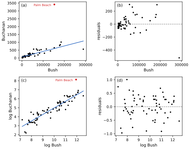
fig_13_2. Download: PDF · SVGSee also (companion course): residual plots and transformations of the response in Section 3.3.3 of Applied Statistical Learning.
13.2 Least Squares and Maximum Likelihood
pp. 212–213 Add the assumption \(\epsilon_i\given X_i\)
\(\mathcal{L}_1\) does not involve \((\beta_0,\beta_1,\sigma)\), so we maximise the conditional likelihood \(\mathcal{L}_2\propto\sigma^{-n}\exp\{-\sum_i(Y_i-\mu_i)^2/(2\sigma^2)\}\), whose logarithm is
\[ \ell(\beta_0,\beta_1,\sigma)=-n\log\sigma-\frac{1}{2\sigma^2}\sum_{i=1}^n\big(Y_i-(\beta_0+\beta_1X_i)\big)^2 . \tag{13.9} \]Theorem 13.7 (least squares is maximum likelihood) p. 213
Under Normal errors the least squares estimator is the maximum likelihood estimator of \((\beta_0,\beta_1)\). The MLE of \(\sigma^2\) is
\[ \hs^2=\frac1n\sum_i\he_i^2, \tag{13.10} \]which differs from the unbiased estimator (13.7) by the factor \((n-2)/n\); common practice is to use (13.7).
Filling the gap 13.3: the maximisation in full, and when the factorisation is legitimate pp. 212–213
(a) For every fixed \(\sigma>0\), (13.9) is maximised over \((\beta_0,\beta_1)\) exactly by the least squares estimates, which do not depend on \(\sigma\). (b) The profile log-likelihood \(-n\log\sigma-\RSS/(2\sigma^2)\) has its unique maximum at \(\sigma^2=\RSS/n\). (c) The maximised log-likelihood, constant included, is
\[ \widehat\ell=-\frac n2\log\Big(\frac{2\pi\,\RSS}{n}\Big)-\frac n2, \]which is what AIC and BIC use in Section 13.6. (d) \(\E(\RSS/n)=\sigma^2(n-2)/n\): the MLE underestimates \(\sigma^2\) by \(2\sigma^2/n\). (e) Dropping \(\mathcal{L}_1\) is legitimate when the distribution of \(X\) does not depend on \((\beta_0,\beta_1,\sigma)\) (the covariates are "ancillary"); if it did, \(\mathcal L_1\) would carry information about the parameters and the conditional MLE would no longer be the full MLE.
Proof
(a) In (13.9) the parameters \((\beta_0,\beta_1)\) enter only through \(-\RSS(\beta_0,\beta_1)/(2\sigma^2)\), which is largest where \(\RSS\) is smallest (Theorem 13.4). (b) Write \(R=\RSS(\hb_0,\hb_1)\) and \(g(\sigma)=-n\log\sigma-R/(2\sigma^2)\); then \(g'(\sigma)=-n/\sigma+R/\sigma^3\) is positive for \(\sigma^2<R/n\) and negative beyond, so \(\sigma^2=R/n\) is the unique maximiser (if \(R>0\), which holds with probability one when \(n\ge3\) and the errors are continuous). (c) Substitute \(\sigma^2=R/n\) into the full log-density \(-\tfrac n2\log(2\pi\sigma^2)-R/(2\sigma^2)\). (d) By Filling the gap 13.2(c). (e) If \(f_X\) depends on a parameter \(\gamma\) unrelated to \((\beta,\sigma)\), the full log-likelihood is \(\log\mathcal L_1(\gamma)+\log\mathcal L_2(\beta,\sigma)\), maximised separately. ∎
In matrix form the same statements are Results 3.1 and 3.2 of Bayesian and Probabilistic Machine Learning and Result 4.4 of Foundations of Deep Learning.
13.3 Properties of the Least Squares Estimators
p. 214 In regression we usually study the estimators conditionally on the covariates \(\Xn=(X_1,\dots,X_n)\), treating them as fixed.
Theorem 13.8 (mean and covariance of \(\hb\)) p. 214
Let \(\hb^\T=(\hb_0,\hb_1)\) be the least squares estimators. Then
\[ \E(\hb\given\Xn)=\begin{pmatrix}\beta_0\\ \beta_1\end{pmatrix},\qquad \V(\hb\given\Xn)=\frac{\sigma^2}{n\,s_X^2}\begin{pmatrix}\frac1n\sum_{i=1}^nX_i^2&-\bX\\ -\bX&1\end{pmatrix}, \tag{13.11} \]where \(s_X^2=n^{-1}\sum_{i=1}^n(X_i-\bX)^2\). Replacing \(\sigma\) by \(\hs\), the estimated standard errors are
\[ \widehat\se(\hb_0)=\frac{\hs}{s_X\sqrt n}\sqrt{\frac{\sum_{i=1}^nX_i^2}{n}}, \tag{13.12} \] \[ \widehat\se(\hb_1)=\frac{\hs}{s_X\sqrt n}. \tag{13.13} \]Filling the gap 13.4: proof of Theorem 13.8 (Exercise 13.2) p. 214
Both estimators are linear in the responses, \(\hb_1=\sum_ic_iY_i\) and \(\hb_0=\sum_id_iY_i\), with weights
\[ c_i=\frac{X_i-\bX}{\Sxx},\qquad d_i=\frac1n-\bX c_i, \]which satisfy \(\sum_ic_i=0\), \(\sum_ic_iX_i=1\), \(\sum_ic_i^2=1/\Sxx\). Means, variances and the covariance then follow from the rules for linear combinations of uncorrelated variables. Only \(\E(\epsilon_i\given\Xn)=0\), \(\V(\epsilon_i\given\Xn)=\sigma^2\) and uncorrelated errors are used: no Normality.
Proof
The identities: \(\sum_i(X_i-\bX)=0\), \(\sum_i(X_i-\bX)X_i\)
Means. \(\E(\hb_1\given\Xn)\)
Variances. \(\V(\hb_1\given\Xn)\)
because \(\Sxx+n\bX^2=\sum_iX_i^2\) and \(\Sxx=ns_X^2\). Covariance. \(\Cov(\hb_0,\hb_1\given\Xn)\)
Theorem 13.9 (consistency, asymptotic normality, intervals and tests) pp. 214–215
Under appropriate conditions (made precise below):
- (consistency) \(\hb_0\toP\beta_0\) and \(\hb_1\toP\beta_1\);
- (asymptotic normality) \((\hb_0-\beta_0)/\widehat\se(\hb_0)\rightsquigarrow\N(0,1)\) and \((\hb_1-\beta_1)/\widehat\se(\hb_1)\rightsquigarrow\N(0,1)\);
- approximate \(1-\alpha\) confidence intervals for \(\beta_0\) and \(\beta_1\) are \[ \hb_0\pm z_{\alpha/2}\,\widehat\se(\hb_0)\quad\text{and}\quad\hb_1\pm z_{\alpha/2}\,\widehat\se(\hb_1); \tag{13.14} \]
- the Wald test of \(H_0:\beta_1=0\) against \(H_1:\beta_1\ne0\) rejects when \(|W|>z_{\alpha/2}\), \(W=\hb_1/\widehat\se(\hb_1)\) (Definition 10.3).
Filling the gap 13.5: what "appropriate conditions" means, with a proof p. 214
Condition on the design, and assume the errors \(\epsilon_1,\epsilon_2,\dots\) are independent and identically distributed with mean 0 and variance \(\sigma^2\in(0,\infty)\) (Normality is not needed).
- Consistency. \(\hb_1\toP\beta_1\) if \(\Sxx\to\infty\); \(\hb_0\toP\beta_0\) if moreover \(\bX^2/\Sxx\to0\).
- Asymptotic normality. If no single design point dominates, \[ \max_{1\le i\le n}\frac{(X_i-\bX)^2}{\Sxx}\to0, \] then \((\hb_1-\beta_1)/\widehat\se(\hb_1)\rightsquigarrow\N(0,1)\); the same holds for \(\hb_0\) when \(\max_id_i^2/\sum_jd_j^2\to0\).
- Random covariates. If the \(X_i\) are themselves iid with \(0<\V(X)<\infty\), all these conditions hold with probability one.
- Exact version. If the errors are Normal, \((\hb_j-\beta_j)/\widehat\se(\hb_j)\) has exactly a \(t\) distribution with \(n-2\) degrees of freedom for every \(n\), so \(t_{n-2,\alpha/2}\) can replace \(z_{\alpha/2}\) in (13.14).
Item 2 is a central limit theorem for weighted sums: without its condition it fails (with \(n-1\) design points at 0 and one at 1, \(\hb_1-\beta_1\)
Proof
(1) \(\hb_1\) is unbiased with variance \(\sigma^2/\Sxx\to0\), so Chebyshev's inequality gives \(\P(|\hb_1-\beta_1|\)
(2) \(\hb_1-\beta_1=\sum_ic_i\epsilon_i\) with \(s_n^2=\V(\sum_ic_i\epsilon_i)\)
Put \(m_n=\max_ic_i^2/\sum_jc_j^2\), which is the displayed condition. Since \(|c_i|\le\sqrt{m_n}\,s_n/\sigma\), the event \(\{|c_i\epsilon_i|>\eta s_n\}\) is contained in \(\{|\epsilon_i|>\eta\sigma/\sqrt{m_n}\}\), and
\[ L_n\le\sum_i\frac{c_i^2}{\sum_jc_j^2}\cdot\frac{\E\big[\epsilon^2\ind\{|\epsilon|>\eta\sigma/\sqrt{m_n}\}\big]}{\sigma^2}=\frac{\E\big[\epsilon^2\ind\{|\epsilon|>\eta\sigma/\sqrt{m_n}\}\big]}{\sigma^2}\to0 \]by dominated convergence, because \(m_n\to0\) and \(\E\epsilon^2<\infty\). Next, \(\hs^2\toP\sigma^2\): by Filling the gap 13.2(c), \((n-2)\hs^2\)
(3) By the strong law, \(\Sxx/n\to\V(X)>0\) and \(\bX\to\E X\), so \(\Sxx\to\infty\) and \(\bX^2/\Sxx\to0\). For the maximum, \(\max_i(X_i-\bX)^2\)
(4) Under Normal errors, \(\hb\) is Normal, \((n-2)\hs^2/\sigma^2\sim\chi^2_{n-2}\), and the two are independent (the matrix proof is Filling the gap 3.1 of Statistical Learning: Theory and Methods); a standard Normal divided by the square root of an independent \(\chi^2_{n-2}/(n-2)\) is \(t_{n-2}\) (see Section 0.6 of the first-year notes). ∎
Example 13.10. p. 215 On the log scale of the election data, a 95 percent interval for the slope is \(0.7298\pm2(0.0360)=(0.658,0.802)\) (book: \((.66,.80)\)), and the Wald statistic for \(H_0:\beta_1=0\) is \(|W|=0.7298/0.0360=20.28\) (book: 20.40), with a \(p\)-value of essentially 0. With \(n=66\) the exact \(t_{64}\) quantile is 1.998, so the "2" in the book's interval is the exact Normal-errors value as well.
See also: the Wald test in general, Section 10.1 of this course; the \(t\) interval and its "2" in Filling the gap 3.3 of Applied Statistical Learning.
13.4 Prediction
p. 215 A new subject has covariate value \(X=x_*\). Its outcome \(Y_*\) is predicted by
\[ \hY_*=\hb_0+\hb_1x_* , \tag{13.15} \]whose variance is \(\V(\hY_*)\)
Theorem 13.11 (prediction interval) p. 215
Let
\[ \widehat\xi_n^{\,2}=\hs^2\Big(\frac{\sum_{i=1}^n(X_i-x_*)^2}{n\sum_i(X_i-\bX)^2}+1\Big). \tag{13.16} \]An approximate \(1-\alpha\) prediction interval for \(Y_*\) is
\[ \hY_*\pm z_{\alpha/2}\,\widehat\xi_n . \tag{13.17} \]Filling the gap 13.6: where \(\widehat\xi_n\) comes from, and why this interval needs Normal errors p. 215
Let \(Y_*=\beta_0+\beta_1x_*+\epsilon_*\), with \(\epsilon_*\) independent of the sample, mean 0 and variance \(\sigma^2\).
- The variance. \(\E(Y_*-\hY_*\given\Xn)=0\) and \[ \V(Y_*-\hY_*\given\Xn)=\sigma^2+\V(\hY_*\given\Xn)=\sigma^2\Big(1+\frac1n+\frac{(x_*-\bX)^2}{\Sxx}\Big), \] which is (13.16) with \(\sigma\) in place of \(\hs\), because \(\sum_i(X_i-x_*)^2=\Sxx+n(\bX-x_*)^2\).
- Normal errors: an exact interval. Then \((Y_*-\hY_*)/\widehat\xi_n\) has exactly the \(t_{n-2}\) distribution, and \(\hY_*\pm t_{n-2,\alpha/2}\widehat\xi_n\) has coverage exactly \(1-\alpha\) for every \(n\); (13.17) is its large-\(n\) version.
- Non-Normal errors: no central limit theorem rescues it. Under the conditions of Filling the gap 13.5, \(\hY_*\toP\beta_0+\beta_1x_*\) and \(\widehat\xi_n\toP\sigma\), so \[ \frac{Y_*-\hY_*}{\widehat\xi_n}\rightsquigarrow\frac{\epsilon_*}{\sigma}, \qquad \P\big(Y_*\in\hY_*\pm z_{\alpha/2}\widehat\xi_n\big)\to\P\big(|\epsilon_*|\le z_{\alpha/2}\sigma\big), \] which equals \(1-\alpha\) only if the error distribution has the Normal's central probability. With Laplace (double exponential) errors the 95% interval covers \(1-e^{-1.96\sqrt2}=0.937\); with uniform errors it covers 1 and is needlessly wide. The interval (13.14) for a coefficient averages many errors and is protected by the central limit theorem; a prediction interval is about one new error and is not.
- The wrong interval. \(\hY_*\pm z_{\alpha/2}s\) with \(s=\widehat\se(\hY_*)\) has coverage about \(2\Phi\big(z_{\alpha/2}/\sqrt{1+\sigma^2/s^2}\big)-1\), which tends to 0 as \(n\to\infty\) because \(s^2=O(1/n)\) (Exercise 13.10(a)).
Proof
(1) \(\hY_*\) is a function of the sample and \(\epsilon_*\) is independent of it, so the variances add: \(\V(Y_*-\hY_*)\)
(2) Under Normality, \(Y_*-\hY_*\) is Normal with mean 0 and variance \(\xi_n^2\) (the formula in (1)), and it is independent of \(\hs^2\): \(\hs^2\) is a function of the residuals, which are independent of \(\hb\) (Filling the gap 13.7), and of \(\epsilon_*\). Since \((n-2)\hs^2/\sigma^2\sim\chi^2_{n-2}\), the ratio \((Y_*-\hY_*)/\widehat\xi_n\) is \(t_{n-2}\).
(3) \(\hY_*-(\beta_0+\beta_1x_*)\)
(4) \(Y_*-\hY_*=(\th-\hY_*)+\epsilon_*\) with \(\th=\beta_0+\beta_1x_*\); the first term is approximately \(\N(0,s^2)\), so \((Y_*-\hY_*)/s\)
The same two intervals, with the \(t\) quantile, are Filling the gap 3.8 of Applied Statistical Learning.
Example 13.12 (election data revisited). p. 216 In Palm Beach, Bush had 152,964 votes and Buchanan 3,411 (certified counts), \(x_*=\log152964=11.938\) and an observed \(\log3411=8.135\). The prediction is \(\hY_*=-2.3185+0.7298\times11.938\)
The 95% prediction interval is \(6.394\pm1.96(0.4307)=(5.549,7.238)\), that is 257 to 1391 votes, which excludes the observed 3,411: Palm Beach lies \((8.135-6.394)/0.4307=4.0\) prediction standard errors above its prediction (two-sided \(p\)-value \(1.4\times10^{-4}\) from \(t_{64}\)). The book instead reports \(\widehat\xi_n=0.093775\), the interval \((6.200,6.578)\), "nearly 20 standard errors" and a vote-scale interval (493, 717): those are the numbers of the interval for the line, \(s\), not of a prediction interval. The conclusion survives the correction, but the evidence is "4 standard errors", not 20 (Notes on the book). Wand et al. (2001) reach the same conclusion with a much finer analysis of the ballots.
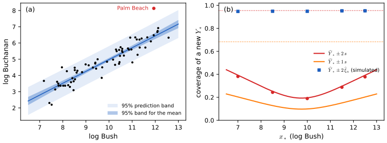
fig_13_s1. Download: PDF · SVGSee also (companion course): the regression bands demo of Applied Statistical Learning draws the same two bands on the Advertising data.
13.5 Multiple Regression
pp. 216–217 Now the covariate is a vector, \(X_i=(X_{i1},\dots,X_{ik})\), and the model is
\[ Y_i=\sum_{j=1}^k\beta_jX_{ij}+\epsilon_i,\qquad i=1,\dots,n, \tag{13.18} \]with \(\E(\epsilon_i\given X_{i1},\dots,X_{ik})\)
Theorem 13.13 (least squares in matrix form) p. 217
Assume the \(k\times k\) matrix \(X^\T X\) is invertible. Then
\[ \hb=(X^\T X)^{-1}X^\T Y, \tag{13.20} \] \[ \V(\hb\given\Xn)=\sigma^2(X^\T X)^{-1}, \tag{13.21} \] \[ \hb\approx\N\big(\beta,\sigma^2(X^\T X)^{-1}\big). \tag{13.22} \]The estimated regression function is \(\hr(x)=\sum_{j=1}^k\hb_jx_j\). An unbiased estimate of \(\sigma^2\) is \(\hs^2=\big(\frac1{n-k}\big)\sum_{i=1}^n\he_i^2\), where \(\he=Y-X\hb\) is the vector of residuals. An approximate \(1-\alpha\) confidence interval for \(\beta_j\) is
\[ \hb_j\pm z_{\alpha/2}\,\widehat\se(\hb_j), \tag{13.23} \]where \(\widehat\se^{\,2}(\hb_j)\) is the \(j\)th diagonal element of \(\hs^2(X^\T X)^{-1}\).
Filling the gap 13.7: proof of Theorem 13.13, and when (13.22) holds p. 217
Assume, given \(X\), uncorrelated errors with mean 0 and variance \(\sigma^2\).
- Normal equations. \(\RSS(b)=\|Y-Xb\|^2\) is minimised exactly by the solutions of \(X^\T Xb=X^\T Y\); if \(X\) has rank \(k\) the solution (13.20) is unique, and \(\RSS(b)=\RSS(\hb)+(b-\hb)^\T X^\T X(b-\hb)\).
- Projection. \(\hY=HY\) with \(H=X(X^\T X)^{-1}X^\T\), which is symmetric, idempotent and has trace \(k\); the residuals \(\he=(I-H)Y=(I-H)\epsilon\) are orthogonal to every column of \(X\).
- Moments. \(\E(\hb\given X)=\beta\), (13.21), and \(\E(\RSS\given X)=\sigma^2(n-k)\), so \(\hs^2\) is unbiased.
- Distribution. Under Normal errors (13.22) is exact: \(\hb\) is Normal with mean \(\beta\) and covariance \(\sigma^2(X^\T X)^{-1}\), independent of \(\hs^2\), with \((n-k)\hs^2/\sigma^2\sim\chi^2_{n-k}\). Without Normality, with iid errors, (13.22) holds asymptotically in the sense that \[ \frac{a^\T(\hb-\beta)}{\{\sigma^2a^\T(X^\T X)^{-1}a\}^{1/2}}\rightsquigarrow\N(0,1)\quad\text{for every fixed }a, \] provided the largest leverage tends to zero, \(\max_ih_{ii}\to0\) (Huber 1973).
Proof
(1) For any \(b\), write \(Y-Xb=(Y-X\hb)+X(\hb-b)\) where \(\hb\) solves the normal equations. The cross term \(2(\hb-b)^\T X^\T(Y-X\hb)\) vanishes by the normal equations, which gives the identity; the second term is \(\ge0\) with equality iff \(X(b-\hb)=0\), i.e. \(b=\hb\) when \(X\) has rank \(k\). A rank-\(k\) \(X\) is exactly the condition for \(X^\T X\) to be invertible (\(X^\T Xv=0\Rightarrow\|Xv\|^2=0\)).
(2) \(H^\T=H\) and \(H^2=X(X^\T X)^{-1}X^\T X(X^\T X)^{-1}X^\T\)
(3) \(\hb=\beta+(X^\T X)^{-1}X^\T\epsilon\), so \(\E\hb=\beta\) and \(\V(\hb)=(X^\T X)^{-1}X^\T(\sigma^2I)X(X^\T X)^{-1}\)
(4) Normal case: \(\hb-\beta\) and \(\he\) are linear in \(\epsilon\) with \(\Cov((X^\T X)^{-1}X^\T\epsilon,(I-H)\epsilon)\)
The same results in the companion course: Results 3.1–3.4 of Statistical Learning: Theory and Methods, which also proves that least squares is the best linear unbiased estimator (Gauss-Markov, Result 3.6).
Example 13.14. pp. 217–218 Crime rates of 47 US states in 1960 (Ehrlich 1973; Vandaele 1978) regressed on ten covariates. The data are those that the book cites, with the response (offences per million inhabitants) divided by 10, which is the scale of the book's coefficients; refitting reproduces the book's table to the printed precision (the book sometimes truncates instead of rounding, as in \(-589.39\) for \(-589.3999\) and 13.24 for 13.2451, and gives some \(t\) values to one decimal):
| Covariate | \(\hb_j\) | \(\widehat\se(\hb_j)\) | \(t\) value | \(p\)-value |
|---|---|---|---|---|
| (Intercept) | −589.40 | 167.59 | −3.52 | 0.001 |
| Age | 1.04 | 0.45 | 2.33 | 0.025 |
| Southern state | 11.29 | 13.25 | 0.85 | 0.399 |
| Education | 1.18 | 0.68 | 1.73 | 0.093 |
| Expenditures | 0.96 | 0.25 | 3.86 | 0.000 |
| Labor | 0.11 | 0.15 | 0.69 | 0.493 |
| Number of males | 0.30 | 0.22 | 1.36 | 0.181 |
| Population | 0.09 | 0.14 | 0.65 | 0.518 |
| Unemployment (14–24) | −0.68 | 0.48 | −1.42 | 0.165 |
| Unemployment (25–39) | 2.15 | 0.95 | 2.26 | 0.030 |
| Wealth | −0.08 | 0.09 | −0.91 | 0.367 |
The "\(t\) value" is the Wald statistic \(W_j=\hb_j/\widehat\se(\hb_j)\) for \(H_0:\beta_j=0\). The printed \(p\)-values are those of the \(t_{36}\) distribution (\(n-k=47-11\)), the exact ones under Normal errors; the Normal approximation of (13.23) would give slightly smaller values (0.020 instead of 0.025 for Age). Two questions follow: should some variables be dropped (Section 13.6), and are these relationships causal (no: Chapter 16 of the book)?
See also (companion courses): the multiple regression table and its standard errors in Filling the gap 3.5 of Applied Statistical Learning; the prostate cancer table in Section 3.2.1 of Statistical Learning: Theory and Methods.
13.6 Model Selection
p. 218 A smaller model may predict better and is simpler. Adding covariates lowers the bias of the predictions and raises their variance; too few covariates underfit, too many overfit. Model selection needs (i) a score for each model and (ii) a search through the models.
pp. 218–219 For \(S\subset\{1,\dots,k\}\) let \(X_S\) be the corresponding columns, \(\hb_S\) the least squares estimate, \(\hr_S\) the fitted regression function and \(\hY_i(S)=\hr_S(X_i)\). The prediction risk is
\[ R(S)=\sum_{i=1}^n\E\big(\hY_i(S)-Y_i^*\big)^2, \tag{13.24} \]where \(Y_i^*\) is a future observation at covariate value \(X_i\), independent of the data. The training error is \(\Rtr(S)=\sum_{i=1}^n(\hY_i(S)-Y_i)^2\).
Theorem 13.15 (the training error is optimistic) p. 219
The training error is a downward-biased estimate of the prediction risk, \(\E\,\Rtr(S)<R(S)\). In fact
\[ \bias\big(\Rtr(S)\big)=\E\,\Rtr(S)-R(S)=-2\sum_{i=1}^n\Cov\big(\hY_i,Y_i\big). \tag{13.25} \]Filling the gap 13.8: proof of (13.25) (Exercise 13.4), its value for least squares, and why \(C_p\) is unbiased p. 219
Fixed design: \(Y_i=\mu_i+\epsilon_i\), uncorrelated errors with variance \(\sigma^2\); \(Y_i^*=\mu_i+\epsilon_i^*\) with fresh errors.
- (13.25) holds for any fitting procedure with finite second moments.
- For least squares on \(|S|\) columns, \(\hY=H_SY\) and \(\sum_i\Cov(\hY_i,Y_i)\)
\({}=\sigma^2\tr H_S\) \({}=\sigma^2|S|\), so the training error is too small by exactly \(2|S|\sigma^2\) on average: \[ \E\,\Rtr(S)=\|(I-H_S)\mu\|^2+(n-|S|)\sigma^2,\qquad R(S)=\|(I-H_S)\mu\|^2+(n+|S|)\sigma^2 . \] The first term is the squared bias of model \(S\); it falls as \(S\) grows, while the variance term \(|S|\sigma^2\) of \(R(S)\) rises. - Hence Mallows' \(C_p\) (13.26) is unbiased for \(R(S)\) whenever \(\E\hs^2=\sigma^2\), which holds when \(\hs^2\) comes from a model that contains the true mean (for example the full model, if it is correct).
- The inequality in Theorem 13.15 is strict exactly when \(\sum_i\Cov(\hY_i,Y_i)>0\), true for least squares with \(|S|\ge1\) but not for every procedure (a fit that ignores the responses has zero optimism).
Proof
(1) Since \(Y_i^*\) is independent of \(\hY_i\) and has the same mean and variance as \(Y_i\),
\[ \E(\hY_i-Y_i^*)^2=\V(\hY_i)+\sigma^2+(\E\hY_i-\mu_i)^2,\qquad \E(\hY_i-Y_i)^2=\V(\hY_i)+\sigma^2-2\Cov(\hY_i,Y_i)+(\E\hY_i-\mu_i)^2 . \]Subtract and sum over \(i\).
(2) \(\Cov(\hY,Y)\)
(3) \(\E C_p=\E\Rtr(S)+2|S|\E\hs^2=R(S)\). If \(\hs^2=\RSS_F/(n-k_F)\) from a model \(F\) with \(\mu=X_F\gamma\) for some \(\gamma\), then \((I-H_F)\mu=0\) and \(\E\RSS_F=\sigma^2(n-k_F)\); otherwise \(\E\hs^2>\sigma^2\).
(4) Immediate from (13.25). ∎
The same covariance formula is Result 7.6 of Statistical Learning: Theory and Methods, where it defines the effective degrees of freedom of any fit.
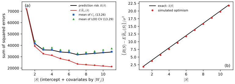
fig_13_s2. Download: PDF · SVGp. 219 The data are used twice, to fit and to assess, which is why the training error is too optimistic, the more so the more parameters are fitted. Mallows' \(C_p\) statistic adds the bias back:
\[ \widehat R(S)=\Rtr(S)+2|S|\hs^2, \tag{13.26} \]where \(|S|\) is the number of terms in \(S\) and \(\hs^2\) is estimated from the full model: lack of fit plus a complexity penalty. p. 220 AIC (Akaike's information criterion, Akaike 1973) chooses \(S\) to maximise
\[ \ell_S-|S|, \tag{13.27} \]with \(\ell_S\) the log-likelihood of model \(S\) at its MLE: goodness of fit minus complexity. (Many programs report \(-2\ell_S+2|S|\), to be minimised; the selected model is the same.)
Filling the gap 13.9: AIC is \(C_p\) (Exercise 13.8), and what R's AIC does pp. 220–222
(a) \(\sigma\) known, or fixed at the full-model \(\hs\). In the Normal linear model
\[ \ell_S-|S|=\text{const}-\frac{\Rtr(S)+2|S|\sigma^2}{2\sigma^2}=\text{const}-\frac{C_p(S)}{2\sigma^2}, \]a strictly decreasing function of \(C_p\): maximising AIC and minimising \(C_p\) select the same model. In the same way
\[ \BIC(S)=\text{const}-\frac{\Rtr(S)+|S|\sigma^2\log n}{2\sigma^2}: \]BIC is \(C_p\) with the penalty 2 per parameter replaced by \(\log n\), which is larger when \(n\ge8\).
(b) \(\sigma\) estimated within each model (the convention of R, used in Example 13.16). With \(\widehat\ell_S\) from Filling the gap 13.3(c), \(-2\widehat\ell_S+2|S|\)
so R's AIC differences are \(C_p\) differences divided by \(\tilde\sigma^2=\Rtr(F)/n\), up to the error of \(\log(1+\delta)\approx\delta\). The two rankings agree among models that fit nearly as well as the full model and can differ otherwise: since \(\log(1+\delta)<\delta\), R's AIC penalises lack of fit less, and its \(\tilde\sigma^2\) is smaller than \(\hs^2\) by the factor \((n-k)/n\). On the crime data \(C_p\) selects Age, Expenditure, Males, U1, U2, and R's AIC adds Education.
Proof
(a) The log-likelihood with \(\sigma\) fixed, maximised by the least squares fit (Theorem 13.7), is
\[ \ell_S=-\tfrac n2\log(2\pi\sigma^2)-\frac{\Rtr(S)}{2\sigma^2},\qquad \ell_S-|S|=-\tfrac n2\log(2\pi\sigma^2)-\frac{\Rtr(S)+2|S|\sigma^2}{2\sigma^2}, \]and similarly with \(\tfrac12|S|\log n\) for BIC. \(\log n>2\iff n>e^2\approx7.39\).
(b) \(\widehat\ell_S\)
The companion course states the same equivalence as Result 6.3 of Applied Statistical Learning.
p. 220 Leave-one-out cross-validation estimates the risk by
\[ \widehat R_{CV}(S)=\sum_{i=1}^n\big(Y_i-\hY_{(i)}\big)^2, \tag{13.28} \]where \(\hY_{(i)}\) is the prediction of \(Y_i\) from the model fitted without observation \(i\). For least squares no refitting is needed:
\[ \widehat R_{CV}(S)=\sum_{i=1}^n\Big(\frac{Y_i-\hY_i(S)}{1-U_{ii}(S)}\Big)^2, \tag{13.29} \]where \(U_{ii}(S)\) is the \(i\)th diagonal element of
\[ U(S)=X_S(X_S^\T X_S)^{-1}X_S^\T . \tag{13.30} \]\(k\)-fold cross-validation splits the data into \(k\) groups (often \(k=10\)), predicts each group from a fit to the others, and adds up the squared prediction errors. For linear regression \(C_p\) and cross-validation usually agree.
Filling the gap 13.10: the leave-one-out shortcut (13.29), and why cross-validation and \(C_p\) agree p. 220
(a) If \(h_{ii}=U_{ii}(S)<1\), deleting observation \(i\) changes the coefficients by
\[ \hb_{(i)}=\hb-\frac{(X^\T X)^{-1}x_i\,\he_i}{1-h_{ii}}, \qquad\text{hence}\qquad Y_i-x_i^\T\hb_{(i)}=\frac{\he_i}{1-h_{ii}}, \]which gives (13.29). (b) Since \(0\le h_{ii}\le1\) and \(\sum_ih_{ii}=|S|\), for small leverages \((1-h_{ii})^{-2}\approx1+2h_{ii}\) and
\[ \widehat R_{CV}(S)\approx\Rtr(S)+2\sum_ih_{ii}\he_i^2\approx\Rtr(S)+2|S|\hs^2=C_p(S) \]when the squared residuals are about \(\hs^2\) on average, uniformly in \(i\). Points of high leverage are where the two differ. On the crime data the full model has \(\widehat R_{CV}=39858.45\) by (13.29) and by 47 refits alike.
Proof
Write \(A=X^\T X\), \(x=x_i\), \(h=x^\T A^{-1}x\). Without observation \(i\), \(X_{(i)}^\T X_{(i)}=A-xx^\T\) and \(X_{(i)}^\T Y_{(i)}=X^\T Y-xY_i\). The Sherman-Morrison formula, \((A-xx^\T)^{-1}\)
Then \(Y_i-x^\T\hb_{(i)}\)
The same identity, with the generalised cross-validation approximation, is Result 7.13 of Statistical Learning: Theory and Methods.
p. 220 BIC (the Bayesian information criterion, Schwarz 1978) chooses the model that maximises
\[ \BIC(S)=\ell_S-\frac{|S|}{2}\log n . \tag{13.31} \]p. 221 With equal prior probabilities \(1/m\) on the models \(S_1,\dots,S_m\) and a smooth prior on the parameters within each model, the posterior probability of a model is approximately \(\P(S_j\given\text{data})\)
Filling the gap 13.11: where the BIC posterior approximation comes from, and what it means p. 221
Let model \(S\) have parameter \(\th\in\R^d\), log-likelihood \(\ell(\th)\) maximised at \(\ht\), and a prior density \(\pi\) that is continuous and positive at the limit of \(\ht\). Under the regularity conditions of Theorem 9.27, the marginal likelihood \(m(S)=\int e^{\ell(\th)}\pi(\th)\,\d\th\) satisfies
\[ \log m(S)=\ell(\ht)-\frac d2\log n+\frac d2\log(2\pi)-\frac12\log\det\widehat J+\log\pi(\ht)+o_P(1)=\BIC(S)+O_P(1), \]with \(\widehat J=-\ell''(\ht)/n\). Bayes' theorem with equal model priors gives \(\P(S_j\given\text{data})\)
Proof sketch
Expand \(\ell(\th)\)
p. 221 Searching. With \(k\) covariates there are \(2^k\) models. If \(k\) is small all can be scored; otherwise a search is needed. Forward stepwise regression starts with no covariates and adds, one at a time, the one that improves the score most, until no addition helps; backward stepwise regression starts from the full model and removes one at a time. Both are greedy and neither is guaranteed to find the best model.
Example 13.16. pp. 221–222 Backward stepwise regression with R's AIC, \(n\log(\RSS/n)+2|S|\) (Filling the gap 13.9(b)), on the crime data. The full model has AIC 310.37. Removing one covariate gives
| removed | Pop | Labor | South | Wealth | Males | U1 | Educ. | U2 | Age | Expend |
|---|---|---|---|---|---|---|---|---|---|---|
| AIC | 308.92 | 308.99 | 309.31 | 309.44 | 310.73 | 310.92 | 312.11 | 314.61 | 314.97 | 324.66 |
so Population goes (the book prints 308 for 308.92; its other entries are these values rounded). The search then removes Southern (307.91), Labor (306.36) and Wealth (306.16), after which every removal increases AIC (the best, Education, gives 306.29). The final model, with the intercept that the book omits, is
\[ \widehat{\text{Crime}}=-565.12+1.24\,\text{Age}+0.75\,\text{Education}+0.87\,\text{Expenditure}+0.34\,\text{Males}-0.86\,\text{U1}+2.31\,\text{U2}, \]the book's model. It says nothing yet about which variables cause crime.
p. 222 A different approach (Zheng and Loh 1995) does not try to predict well but to find the true model, the largest sub-model whose coefficients are all nonzero (the book's "smallest" is corrected in the author's errata), assuming that some \(\beta_j\) are exactly zero; it needs only \(k+1\) fits instead of a search.
Algorithm 13.A (the Zheng-Loh method) p. 222
- Fit the full model with all \(k\) covariates; let \(W_j=\hb_j/\widehat\se(\hb_j)\) be the Wald statistic for \(H_0:\beta_j=0\).
- Order them by absolute value, \(|W_{(1)}|\)
\({}\ge|W_{(2)}|\) \({}\ge\dots\) \({}\ge|W_{(k)}|\). - Let \(\widehat\jmath\) minimise \(\RSS(j)+j\hs^2\log n\), where \(\RSS(j)\) is the residual sum of squares of the model with the \(j\) largest \(|W|\).
- Choose the model with those \(\widehat\jmath\) covariates.
(The penalty \(j\log n\) is one of a family of penalties allowed by Zheng and Loh.)
Filling the gap 13.12: why the Zheng-Loh method finds the true model pp. 222–223
Assume a fixed number \(k\) of covariates (the intercept always included), iid errors with variance \(\sigma^2\), \(X^\T X/n\to\Sigma\) positive definite, and let \(T=\{j:\beta_j\ne0\}\). Then \(\P(\text{the method selects }T)\to1\). Two facts drive it: the Wald statistics of true covariates grow like \(\sqrt n\) while the others stay bounded, so the ordering puts \(T\) first; and along that ordering, dropping a true covariate costs order \(n\) in RSS, while adding a null one saves only \(O_P(1)\), against a penalty step of \(\hs^2\log n\), which is between the two.
Proof
Ordering. \(\widehat\se(\hb_j)^2\)
Under-fitting. On \(E_n\), for \(j<|T|\) the model omits some true covariate. Its RSS exceeds that of the true model by \(\|(H_T-H_j)Y\|^2\)
Over-fitting. For \(j>|T|\) the model contains the truth, so \(\RSS(|T|)-\RSS(j)\)
Note what is and is not claimed: the method finds the true model, but it is not designed to minimise prediction risk, and in finite samples it can drop real but weak covariates (on the crime data it keeps only Expenditure and Age).
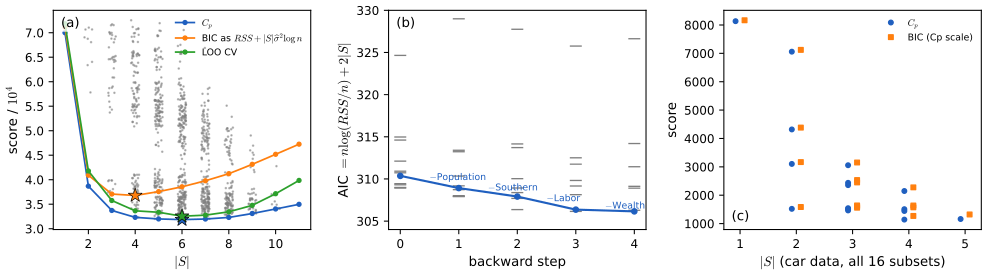
fig_13_s3. Download: PDF · SVGOn the crime data the scores give (exhaustive search over all 1024 models, \(|S|\) counting the intercept):
| score | selected covariates | \(|S|\) |
|---|---|---|
| \(C_p\) (13.26), AIC (13.27) with \(\hs\) fixed, leave-one-out CV (13.29) | Age, Expenditure, Males, U1, U2 | 6 |
| R's AIC (exhaustive and backward) | Age, Education, Expenditure, Males, U1, U2 | 7 |
| BIC (13.31), either form | Age, Expenditure, Males | 4 |
| Zheng-Loh (Algorithm 13.A) | Expenditure, Age | 3 |
See also (companion courses): best subset and stepwise selection in Algorithms 6.2 and 6.3 of Applied Statistical Learning, with its subset selection demo; the optimism by simulation in the optimism and Cp demo of Statistical Learning: Theory and Methods.
13.7 Logistic Regression
p. 223 For a binary response \(Y_i\in\{0,1\}\) and a \(k\)-dimensional covariate, the logistic regression model is
\[ p_i\equiv p_i(\beta)\equiv\P(Y_i=1\given X=x)=\frac{e^{\beta_0+\sum_{j=1}^k\beta_jx_{ij}}}{1+e^{\beta_0+\sum_{j=1}^k\beta_jx_{ij}}}, \tag{13.32} \]or equivalently
\[ \logit(p_i)=\beta_0+\sum_{j=1}^k\beta_jx_{ij}, \tag{13.33} \] \[ \logit(p)=\log\Big(\frac{p}{1-p}\Big). \tag{13.34} \]The name comes from the logistic function \(e^x/(1+e^x)\) (Figure 13.3). pp. 223–224 Since \(Y_i\given X_i=x_i\sim\Bern(p_i)\), the conditional likelihood is
\[ \mathcal L(\beta)=\prod_{i=1}^np_i(\beta)^{Y_i}\big(1-p_i(\beta)\big)^{1-Y_i}. \tag{13.35} \]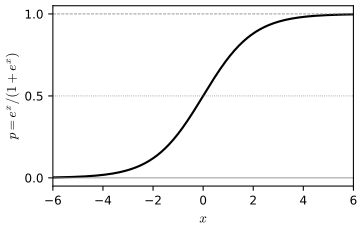
fig_13_3. Download: PDF · SVGp. 224 The MLE has no closed form and is computed numerically, by a fast algorithm called reweighted least squares. Below, \(x_i\) includes a leading 1, \(X\) is the \(n\times(k+1)\) matrix with rows \(x_i^\T\), \(\eta_i=x_i^\T\beta\) and \(W=\mathrm{diag}\{p_i(1-p_i)\}\).
Algorithm 13.B (reweighted least squares, corrected) p. 224
Choose a starting value \(\beta^0\) (for example \(0\)) and compute \(p_i^0\) by (13.32). For \(s=0,1,2,\dots\) until convergence:
- Set \(Z_i=\logit(p_i^s)+\dfrac{Y_i-p_i^s}{p_i^s(1-p_i^s)}\), \(i=1,\dots,n\) (the "working response").
- Let \(W\) be diagonal with \((i,i)\) element \(p_i^s(1-p_i^s)\).
- Set \(\beta^{s+1}=(X^\T WX)^{-1}X^\T WZ\): a weighted linear regression of \(Z\) on \(X\).
The book prints \(X^\T WY\) in step 3 and calls it a regression "of \(Z\) on \(Y\)"; with \(Y\) the iteration does not converge to the MLE. The correction is listed in the author's errata.
Filling the gap 13.13: score, Fisher information, existence of the MLE, and why the algorithm is Newton's method p. 224
- Score and Hessian. \(\ell(\beta)\)
\({}=\sum_i\{Y_i\eta_i-\log(1+e^{\eta_i})\}\) has gradient \(X^\T(Y-p)\) and Hessian \(-X^\T WX\). So \(\ell\) is concave, strictly if \(X\) has full column rank, and the Fisher information \(I(\beta)=X^\T WX\) equals the observed information (it does not involve \(Y\)). - Existence. The MLE exists, and is then unique, if and only if the two classes are not (quasi-)separated: there is no \(b\ne0\) with \(x_i^\T b\ge0\) whenever \(Y_i=1\) and \(x_i^\T b\le0\) whenever \(Y_i=0\) (Albert and Anderson 1984). With separation, \(\ell(tb)\) increases as \(t\to\infty\) and the coefficients run off to infinity.
- Newton = reweighted least squares. Newton's step \(\beta+(X^\T WX)^{-1}X^\T(Y-p)\) equals \((X^\T WX)^{-1}X^\T WZ\) with the working response of Algorithm 13.B. Near the MLE it converges quadratically (Filling the gap 9.23); on the CORIS data it reaches the maximum to \(10^{-8}\) in 4 steps from \(\beta=0\).
- Monotone alternatives. Because \(p(1-p)\le\tfrac14\), \(\ell(\beta+\delta)\)
\({}\ge\ell(\beta)+\delta^\T X^\T(Y-p)-\tfrac18\delta^\T X^\T X\delta\); maximising the bound gives \(\beta\leftarrow\beta+4(X^\T X)^{-1}X^\T(Y-p)\) (Boehning and Lindsay 1988), which never decreases \(\ell\) and needs only one matrix inverse, but converges linearly. Gradient ascent with step \(4/\lambda_{\max}(X^\T X)\) is also monotone, but its speed depends on the units of the covariates (Figure 13.S5).
Proof
(1) From (13.35), \(\ell=\sum_i\{Y_i\log p_i+(1-Y_i)\log(1-p_i)\}\)
(2) Each term of \(\ell\) is \(\le0\). If \(b\) separates, every term of \(\ell(tb)\) is nondecreasing in \(t\) (for \(Y_i=1\) it is \(-\log(1+e^{-t\,x_i^\T b})\), for \(Y_i=0\) it is \(-\log(1+e^{t\,x_i^\T b})\)), so a maximiser along the ray cannot be finite unless all \(x_i^\T b=0\), impossible for \(b\ne0\) when \(X\) has full rank; hence no MLE. If no \(b\ne0\) separates, then for every direction \(b\) some term has the wrong sign and tends to \(-\infty\) along \(tb\), so \(\ell(tb)\to-\infty\) along every ray. A concave function with this property has bounded superlevel sets (they are convex and contain no ray), so the continuous \(\ell\) attains its maximum, uniquely by strict concavity.
(3) \((X^\T WX)^{-1}X^\T WZ\)
(4) By Taylor's theorem with the Hessian bound \(-X^\T WX\succeq-\tfrac14X^\T X\), \(\ell(\beta+\delta)\)
The same derivation is Result 4.8 of Statistical Learning: Theory and Methods and Algorithm 4.2 of Bayesian and Probabilistic Machine Learning.
p. 224 The Fisher information matrix \(I\) is also obtained numerically, and the estimated variance of \(\hb_j\) is the \((j,j)\) element of \(J=I^{-1}\) (the book says "standard error"; corrected in the author's errata). Model selection is usually done with AIC, \(\ell_S-|S|\).
Filling the gap 13.14: why \(I(\hb)^{-1}\) gives the standard errors, and Wald against likelihood ratio p. 224
Let \((X_i,Y_i)\) be iid with \(\E\|X\|^2<\infty\), the model (13.32) correct, and \(\mathcal I=\E[p(X)(1-p(X))XX^\T]\) positive definite. Then the MLE exists with probability tending to one, and
\[ \sqrt n(\hb-\beta)\rightsquigarrow\N(0,\mathcal I^{-1}),\qquad\text{so}\qquad \hb\approx\N\big(\beta,(X^\T\widehat WX)^{-1}\big), \]with \(\widehat W\) evaluated at \(\hb\). Hence \(\widehat\se(\hb_j)\)
Proof
The conditional log-likelihood is a sum of iid terms \(Y\eta-\log(1+e^\eta)\) whose score has mean zero and covariance \(\mathcal I\) and whose Hessian has mean \(-\mathcal I\). By concavity, consistency follows from pointwise convergence of \(\ell(\beta)/n\) to a strictly concave limit maximised at the true \(\beta\) (a convexity lemma replaces the compactness argument), and the expansion \(0=\ell'(\hb)\)
Example 13.17. pp. 224–225 The Coronary Risk-Factor Study (CORIS; Rousseauw et al. 1983): 462 men aged 15 to 64 from three rural areas of South Africa; \(Y=1\) for the 160 with coronary heart disease. The nine covariates are systolic blood pressure, cumulative tobacco (kg), low density lipoprotein cholesterol, adiposity, family history of heart disease, type-A behaviour, obesity, current alcohol consumption and age. The exact MLE (Newton converges in 7 steps to \(10^{-10}\); \(-2\ell=472.14\)) gives
| Covariate | \(\hb_j\) | \(\widehat\se\) | \(W_j\) | Wald \(p\) | LRT \(\lambda_j\) | LRT \(p\) |
|---|---|---|---|---|---|---|
| Intercept | −6.151 | 1.308 | −4.701 | 0.000 | 23.92 | 0.000 |
| sbp | 0.007 | 0.006 | 1.135 | 0.256 | 1.30 | 0.255 |
| tobacco | 0.079 | 0.027 | 2.984 | 0.003 | 9.53 | 0.002 |
| ldl | 0.174 | 0.060 | 2.915 | 0.004 | 8.93 | 0.003 |
| adiposity | 0.019 | 0.029 | 0.635 | 0.526 | 0.41 | 0.525 |
| famhist | 0.925 | 0.228 | 4.061 | 0.000 | 16.75 | 0.000 |
| typea | 0.040 | 0.012 | 3.214 | 0.001 | 10.91 | 0.001 |
| obesity | −0.063 | 0.044 | −1.422 | 0.155 | 2.09 | 0.148 |
| alcohol | 0.000 | 0.004 | 0.027 | 0.978 | 0.00 | 0.978 |
| age | 0.045 | 0.012 | 3.728 | 0.000 | 14.39 | 0.000 |
The slopes agree with the book's to the printed precision; the intercept differs slightly (book: −6.145 with standard error 1.300), several standard errors are larger here in the third decimal (ldl 0.060 against 0.059, famhist 0.228 against 0.227), and the book's Wald statistics are 0.2% to 0.8% larger (for example 4.738 against 4.701), as if its fit had stopped slightly before convergence; the fit above agrees with an independent library fit to \(10^{-14}\). Systolic blood pressure is not significant and obesity has a negative sign: this does not mean that blood pressure does not cause heart disease, only that, given the other eight variables, it adds little to the prediction (on its own its Wald statistic is 4.0). Association is not causation (Chapter 16 of the book). Family history multiplies the odds of heart disease by \(e^{0.925}=2.52\), other factors equal.
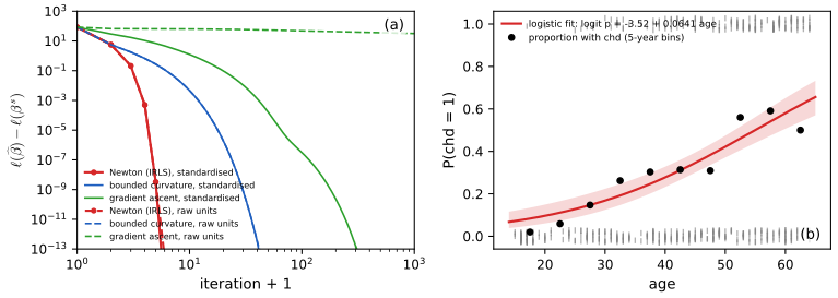
fig_13_s5. Download: PDF · SVGSee also (companion courses): the same data as the South African heart disease study in Section 4.4.2 of Statistical Learning: Theory and Methods, with its IRLS demo; the logistic likelihood in Result 4.1 of Applied Statistical Learning.
13.8 Bibliographic Remarks
p. 225 The book recommends Weisberg (1985) for a short account of linear regression and Hastie, Tibshirani and Friedman (2001) for a data-mining view. AIC is due to Akaike (1973), BIC to Schwarz (1978), \(C_p\) to Mallows (1973), and the selection method of Algorithm 13.A to Zheng and Loh (1995). On logistic regression the book cites Agresti (1990) and Dobson (2001). The leave-one-out identity goes back to Allen (1974) and Stone (1974); the asymptotic normality of least squares under the leverage condition is Huber (1973); the bounded-curvature algorithm is Boehning and Lindsay (1988).
13.9 Appendix
pp. 225–226 The Akaike information criterion. Consider models \(M_1,M_2,\dots\); let \(\widehat f_j(x)=f(x;\hb_j)\) be the density fitted by maximum likelihood in model \(M_j\). Measure the loss by the Kullback-Leibler distance \(D(f,g)=\int f\log(f/g)\). Since \(D(f,\widehat f)=c-A(f,\widehat f)\) with \(c=\int f\log f\) free of \(\widehat f\) and \(A(f,\widehat f)\)
Theorem 13.18 (AIC is approximately unbiased) p. 226
\(\AIC(M_j)=\ell_j(\hb_j)-|M_j|\) is an approximately unbiased estimate of \(n\,a(f,\widehat f_j)\): \(\E\{\ell_j(\hb_j)\}-n\,\E\{A(f,\widehat f_j)\}\)
Filling the gap 13.15: Akaike's bias calculation p. 226
Let \(X_1,\dots,X_n\) be iid with density \(f=f(\cdot;\th_0)\) in a regular \(d\)-parameter model (the model is correct), \(\ell(\th)=\sum_i\log f(X_i;\th)\), \(\ht\) the MLE, \(g(\th)=\int f\log f(\cdot;\th)\), and \(I\) the Fisher information at \(\th_0\). Then, to first order,
\[ \E\,\ell(\ht)\approx n\,g(\th_0)+\frac d2,\qquad n\,\E\,g(\ht)\approx n\,g(\th_0)-\frac d2,\qquad\text{so}\qquad \E\{\ell(\ht)-d\}\approx n\,\E\,g(\ht)=n\,a(f,\widehat f). \]The fitted log-likelihood is too high by \(d/2\) because \(\ht\) is tuned to the sample, and the truth scores \(d/2\) higher than \(\ht\) on new data because \(\ht\) misses \(\th_0\): the two halves add to \(d\). If the model is wrong, \(d\) is replaced by \(\tr(\mathcal I^{-1}K)\), with \(\mathcal I\) minus the expected Hessian and \(K\) the covariance of the score at the best-fitting parameter (Takeuchi 1976); for a correct model \(\mathcal I=K\) and the trace is \(d\).
Derivation
New data. \(g\) is maximised at \(\th_0\) with \(g''(\th_0)=-I\) (Gibbs' inequality and the information identity, Theorem 9.17). Taylor's theorem: \(g(\ht)\approx g(\th_0)-\tfrac12(\ht-\th_0)^\T I(\ht-\th_0)\). Since \(\sqrt n(\ht-\th_0)\rightsquigarrow\N(0,I^{-1})\) (Theorem 9.27), \(n(\ht-\th_0)^\T I(\ht-\th_0)\rightsquigarrow\chi^2_d\), with mean \(d\); so \(n\E g(\ht)\approx ng(\th_0)-d/2\).
Same data. Expand \(\ell\) about \(\ht\), where \(\ell'(\ht)=0\): \(\ell(\th_0)\)
The companion course gives the same expansion in the language of in-sample error: Filling the gap 7.3 of Statistical Learning: Theory and Methods.
Two remarks on the book's wording. "Estimate \(a(f,\widehat f)\) by \(\sum_x\widehat f(x)\log\widehat f(x)\)" should read: by the average log-likelihood of the observed data, \(n^{-1}\sum_i\log\widehat f(X_i)\). And the bias "approximately equal to \(|M_j|\)" refers to the whole-sample log-likelihood \(\ell(\hb)\); per observation it is \(|M_j|/n\). In linear regression with known \(\sigma\), \(-2\sigma^2\) times AIC is \(C_p\) up to a constant (Filling the gap 13.9), so Theorem 13.18 and the unbiasedness of \(C_p\) (Filling the gap 13.8) are the same fact.
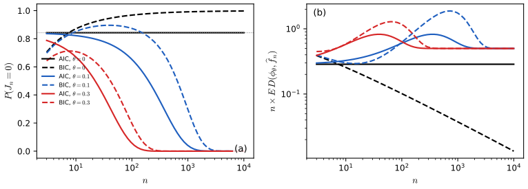
fig_13_s4. Download: PDF · SVGNotes on the book
Several slips of Chapter 13 are in the author's errata lists; the others are mine, each with the evidence.
Page 216, Example 13.12: the "prediction interval" is the interval for the line
The book's \(\widehat\xi_n=0.093775\) cannot be (13.16): by definition \(\widehat\xi_n\ge\hs\), and the residual standard deviation on the log scale is \(\hs=0.42\) (the residuals in Figure 13.2(d) range over about \(\pm1\); also \(\hs=\widehat\se(\hb_1)s_X\sqrt n\)
Page 215, Theorem 13.11: the prediction interval is approximate only for Normal-like errors
Unlike (13.14), (13.17) is not justified by large samples: its coverage tends to \(\P(|\epsilon|\le z_{\alpha/2}\sigma)\), the error distribution's own central probability (Filling the gap 13.6(3)). Under Normal errors the exact interval uses \(t_{n-2}\).
Page 224: the reweighted least squares algorithm and the standard errors
Step 3 should be \(\beta^{s}=(X^\T WX)^{-1}X^\T WZ\), "a weighted linear regression of \(Z\) on \(X\)", and the \((j,j)\) element of \(J=I^{-1}\) is the variance, not the standard error, of \(\hb_j\). Both are listed in the author's errata. Also, the iterate on the left of step 3 should carry the index \(s+1\).
Page 222: the Zheng-Loh "true model" is the largest sub-model with nonzero coefficients
The book says "smallest"; the true model is the set of all covariates whose coefficients are not zero. Listed in the author's errata.
Page 219, Theorem 13.15 and (13.25)
The sum in (13.25) runs over \(i=1,\dots,n\) (the upper limit is missing), and the strict inequality \(\E\Rtr(S)<R(S)\) needs \(\sum_i\Cov(\hY_i,Y_i)>0\), which holds for least squares (it equals \(|S|\sigma^2\)) but not for every fitting rule (Filling the gap 13.8). Not in the errata lists.
Page 217, Theorem 13.13: the sign of the residuals
The residual vector is \(\he=Y-X\hb\), as in (13.4); the book writes \(X\hb-Y\). Harmless for \(\hs^2\), which uses squares. Not in the errata lists; the index slip \(X_{1i},\dots,X_{ki}\) on page 216 is in the second errata list.
Pages 221–222: three small points about BIC and Example 13.16
(1) "The BIC score is identical to Mallows \(C_p\) except that it puts a more severe penalty": true with \(\sigma\) fixed, and the penalty is more severe only for \(n\ge8\) (\(\log n>2\)). (2) In Example 13.16 the AIC after removing Population is 308.92, printed as 308 although the other entries are rounded (309 would be consistent); and "the same is" should be "the same as" (second errata list). (3) The final model is printed without its intercept, \(-565.12\).
Pages 210–211 and 225: data details (not errors)
The line of Figure 13.1 and Example 13.5 is reproduced exactly by the 42 stars with log temperature at least 4.0, the range of the book's plot. The election estimates of Example 13.6 are reproduced to about 1% with the certified county returns (the book's counts are an earlier vintage). The CORIS estimates of Example 13.17 agree except for small differences in the intercept and the standard errors.
Other slips listed in the author's errata
Page 210, line 2: \(\epsilon_i\) is defined in (13.2). Page 212: the bottom panels of Figure 13.2 should be labelled log(Bush) and log(Buchanan). Page 219: "second measure" should be "second measures". Page 225, last line: a missing parenthesis in \(\E(D(f,\widehat f))\). Page 228: a notational slip in \(\widehat\xi_n\) in Exercise 13.10. In the appendix (p. 226) the naive estimate of \(a(f,\widehat f)\) should be the average log-likelihood of the data (see the remark after Filling the gap 13.15; this one is mine).
13.10 Exercises
All eleven exercises of Chapter 13 (Wasserman, 2004, pp. 226–229), restated in my own words, with complete solutions (hidden).
Exercise 13.1. Prove Theorem 13.4.
Solution
See Filling the gap 13.2: minimise over \(b_0\) for fixed \(b_1\), then over \(b_1\); uniqueness from \(\Sxx>0\); and \(\E\RSS=(n-2)\sigma^2\) from the decomposition \(\RSS=\sum_i(\epsilon_i-\bar\epsilon)^2-(\hb_1-\beta_1)^2\Sxx\).
Exercise 13.2. Prove the standard error formulas of Theorem 13.8, treating the \(X_i\) as fixed constants.
Solution
See Filling the gap 13.4: write \(\hb_1=\sum_ic_iY_i\), \(\hb_0=\sum_id_iY_i\) with \(c_i=(X_i-\bX)/\Sxx\), \(d_i=1/n-\bX c_i\), and compute \(\sigma^2\sum c_i^2\), \(\sigma^2\sum d_i^2\), \(\sigma^2\sum c_id_i\). The same matrix can be read off \(\sigma^2(X^\T X)^{-1}\) with \(X=[\mathbf 1,x]\): \(X^\T X=\begin{pmatrix}n&\sum X_i\\ \sum X_i&\sum X_i^2\end{pmatrix}\) has determinant \(n\Sxx\), and its inverse is \(\frac1{n\Sxx}\begin{pmatrix}\sum X_i^2&-n\bX\\ -n\bX&n\end{pmatrix}\), which is (13.11) since \(\Sxx=ns_X^2\).
Exercise 13.3. In the regression through the origin \(Y_i=\beta X_i+\epsilon_i\), find the least squares estimate of \(\beta\), its standard error, and conditions for consistency.
Solution
\(\RSS(b)=\sum_i(Y_i-bX_i)^2\) has derivative \(-2\sum_iX_i(Y_i-bX_i)\), so \(\hb=\sum_iX_iY_i/\sum_iX_i^2\) (if some \(X_i\ne0\)). Given the \(X_i\), \(\hb=\beta+\sum_iX_i\epsilon_i/\sum_iX_i^2\), so \(\E\hb=\beta\) and \(\V(\hb)=\sigma^2/\sum_iX_i^2\). The hat matrix \(xx^\T/\|x\|^2\) has trace 1, so \(\E\RSS=(n-1)\sigma^2\) and \(\hs^2=\RSS/(n-1)\); hence
\[ \widehat\se(\hb)=\frac{\hs}{\sqrt{\sum_iX_i^2}} . \]Consistency: \(\hb\toP\beta\) if \(\sum_{i=1}^nX_i^2\to\infty\) (Chebyshev). The condition is also necessary when the errors are Normal, since then \(\hb\sim\N(\beta,\sigma^2/\sum X_i^2)\) exactly. With iid random covariates, \(\sum X_i^2\sim n\E X^2\to\infty\) whenever \(X\) is not identically 0. Asymptotic normality needs in addition \(\max_iX_i^2/\sum_jX_j^2\to0\) (Filling the gap 13.5).
Exercise 13.4. Prove (13.25).
Solution
See Filling the gap 13.8(1): expand \(\E(\hY_i-Y_i^*)^2\) and \(\E(\hY_i-Y_i)^2\) into variance and squared bias; they differ only by \(-2\Cov(\hY_i,Y_i)\), because \(Y_i^*\) is independent of \(\hY_i\) while \(Y_i\) is not. For least squares the sum is \(-2|S|\sigma^2\).
Exercise 13.5. In simple linear regression, construct a Wald test of \(H_0:\beta_1=17\beta_0\) against \(H_1:\beta_1\ne17\beta_0\).
Solution
Let \(\th=\beta_1-17\beta_0\), so \(H_0:\th=0\). The estimate \(\ht=\hb_1-17\hb_0\) is unbiased with variance, from (13.11),
\[ \V(\ht)=\V(\hb_1)+289\V(\hb_0)-34\Cov(\hb_0,\hb_1)=\frac{\sigma^2}{ns_X^2}\Big(1+34\bX+\frac{289}n\sum_iX_i^2\Big)=\frac{\sigma^2}{ns_X^2}\cdot\frac1n\sum_i(1+17X_i)^2 . \]With \(\hs\) in place of \(\sigma\), \(\widehat\se(\ht)\)
\({}=\dfrac{\hs}{s_X\sqrt n}\Big\{\frac1n\sum_i(1+17X_i)^2\Big\}^{1/2}\), and the Wald test rejects \(H_0\) at level \(\alpha\) when \(|W|>z_{\alpha/2}\), \(W=(\hb_1-17\hb_0)/\widehat\se(\ht)\). It has asymptotic size \(\alpha\) by Theorem 13.9 (any fixed linear combination of \(\hb\) is asymptotically Normal, Filling the gap 13.7(4)); with Normal errors \(W\sim t_{n-2}\) exactly under \(H_0\). Equivalently, write the model as \(Y_i=\beta_0(1+17X_i)+\th X_i+\epsilon_i\) and test the coefficient of \(X_i\). Exercise 13.6. Using the car mileage data (82 cars): (a) regress MPG on horsepower (HP), summarise, and plot the data with the fitted line; (b) repeat with log(MPG) as the response and compare.
Solution
(a) \(\widehat{\text{MPG}}\)
\({}=50.07-0.1390\,\text{HP}\), standard errors 1.57 and 0.0121, \(W=-11.5\), \(\hs=6.17\), \(R^2=0.624\). The slope is clearly nonzero, but the residuals against the fitted values are U-shaped (Figure 13.S6(b)): the fit overpredicts in the middle and underpredicts the most and least powerful cars, and the spread grows with the fitted value. A straight line in HP is the wrong shape. (b) \(\widehat{\log\text{MPG}}\)
\({}=4.013-0.004589\,\text{HP}\), standard errors 0.040 and 0.00031, \(W=-14.9\), \(\hs=0.158\), \(R^2=0.734\). Each extra horsepower lowers mileage by about \(100(1-e^{-0.004589})=0.46\%\). The log scale stabilises the spread and fits better, though some curvature remains (a term in HP\(^2\) or log HP would remove most of it). Since the responses differ, compare the two through the residual plots and \(R^2\), not through \(\hs\). 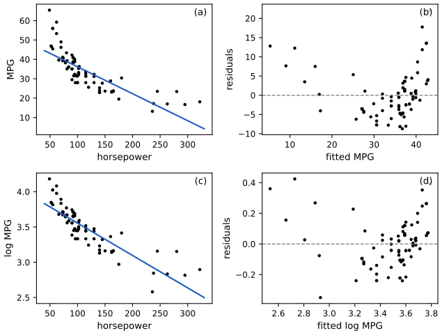
Figure 13.S6 (supplementary). Exercise 13.6: MPG (a) and log MPG (c) against horsepower with the least squares lines, and the residuals against the fitted values (b, d). Not a figure of the book. Code: ch13_regression.py, fig_13_s6. Download: PDF · SVGExercise 13.7. With the car mileage data: (a) regress MPG on all the other variables (cab volume VOL, HP, top speed SP, weight WT) and summarise; (b) select a sub-model by Mallows' \(C_p\) with (i) forward and (ii) backward stepwise search; (c) apply the Zheng-Loh method and compare; (d) score all possible regressions with \(C_p\) and BIC and compare.
Solution
(a)
\[ \widehat{\text{MPG}}=192.44-0.0156\,\text{VOL}+0.392\,\text{HP}-1.295\,\text{SP}-1.860\,\text{WT}, \]with standard errors 23.53, 0.0228, 0.0814, 0.245, 0.213 and Wald statistics 8.18, \(-0.69\), 4.82, \(-5.29\), \(-8.72\); \(\hs=3.65\), \(R^2=0.873\). Weight and top speed lower mileage; given them, horsepower has a positive coefficient, because HP and SP are strongly correlated (powerful cars are fast), so the HP coefficient compares cars of equal speed and weight. Cab volume adds nothing.
(b) With \(\hs^2=13.34\) from the full model: forward search adds WT (\(C_p=1519.4\)), SP (1463.1), HP (1140.4), and stops (adding VOL gives 1160.8); backward search removes VOL and stops. Both give {HP, SP, WT}.
(c) The |W| order is WT (8.72), SP (5.29), HP (4.82), VOL (0.69); \(\RSS(j)+j\hs^2\log82\) is 8107.5, 1524.8, 1500.6, 1210.0, 1262.6 for \(j=0,\dots,4\), minimised at \(j=3\): the same model.
(d) Over all 16 models, \(C_p\) is smallest for {HP, SP, WT} (1140.4; the full model is second, 1160.8) and so is BIC (on the \(C_p\) scale 1268.8 against 1321.4; R's BIC 225.43 against 229.33), as in Figure 13.S3(c). Here every method agrees, because VOL is useless and the other three are strong. On the log scale the two scores part: \(C_p\) keeps {HP, SP, WT}, BIC drops HP.
▶ DemoExercise 13.7 in the browserSwitch between forward, backward and exhaustive search and between the six scores.Exercise 13.8. In the linear regression model with Normal errors and known \(\sigma\), show that the model with the highest AIC (13.27) is the model with the lowest Mallows \(C_p\).
Solution
See Filling the gap 13.9(a): \(\ell_S-|S|\)
\({}=-\tfrac n2\log(2\pi\sigma^2)-C_p(S)/(2\sigma^2)\), with \(C_p\) computed with the known \(\sigma^2\); a strictly decreasing function of \(C_p\) is maximised where \(C_p\) is minimised. Exercise 13.9. Let \(X_1,\dots,X_n\) be iid and compare \(M_0:\N(0,1)\) with \(M_1:\N(\th,1)\), \(\th\in\R\), by AIC: \(\AIC_0=\ell_n(0)\), \(\AIC_1=\ell_n(\ht)-1\), and \(J_n\) is the model with the larger score. (a) Find \(\lim_n\P(J_n=0)\) when \(\th=0\) and when \(\th\ne0\). (b) Let \(\widehat f_n=\phi_0\) if \(J_n=0\) and \(\phi_{\ht}\) if \(J_n=1\). Show that \(D(\phi_0,\widehat f_n)\toP0\) when \(\th=0\) and \(D(\phi_\th,\widehat f_n)\toP0\) when \(\th\ne0\): AIC estimates the density consistently even though it "overfits". (c) Repeat for BIC, the log-likelihood minus \((p/2)\log n\).
Solution
\(\ell_n(\th)\)
\({}=-\tfrac12\sum_i(X_i-\th)^2+c\), \(\ht=\bX\), and \(\sum(X_i-0)^2-\sum(X_i-\bX)^2=n\bX^2\), so \(\AIC_1-\AIC_0=\tfrac12n\bX^2-1\): \(J_n=0\) iff \(n\bX^2<2\) (ties have probability 0). Note \(\sqrt n\bX\sim\N(\sqrt n\th,1)\) exactly. (a) If \(\th=0\), \(n\bX^2\sim\chi^2_1\) for every \(n\), so \(\P(J_n=0)=\P(\chi^2_1<2)=0.8427\), and the limit is 0.8427, not 1. If \(\th\ne0\), \(\P(J_n=0)\)
\({}=\Phi(\sqrt2-\sqrt n\th)-\Phi(-\sqrt2-\sqrt n\th)\) \({}\to0\). (b) For Normal densities with variance 1, \(D(\phi_a,\phi_b)=(a-b)^2/2\). If \(\th=0\): \(D(\phi_0,\widehat f_n)\)
\({}=\ind\{J_n=1\}\bX^2/2\) \({}\le\bX^2/2\) \({}\toP0\), although \(J_n=1\) with probability 0.157. If \(\th\ne0\): \(D(\phi_\th,\widehat f_n)\) \({}=\ind\{J_n=0\}\th^2/2+\ind\{J_n=1\}(\bX-\th)^2/2\), and both terms tend to 0 in probability, the first because \(\P(J_n=0)\to0\), the second because \(\bX\toP\th\). Under \(\th=0\) the expected loss is \(\E[\chi^2_1\ind\{\chi^2_1>2\}]/(2n)\) \({}=\P(\chi^2_3\) \({}>2)/(2n)\) \({}=0.286/n\). (c) \(\BIC_1-\BIC_0\)
\({}=\tfrac12n\bX^2-\tfrac12\log n\), so \(J_n=0\) iff \(n\bX^2<\log n\). If \(\th=0\), \(\P(J_n=0)=\P(\chi^2_1<\log n)\to1\): BIC is consistent. If \(\th\ne0\), \(\P(J_n=0)\) \({}=\P(|\N(\sqrt n\th,1)|\) \({}<\sqrt{\log n})\) \({}\to0\) because \(\sqrt n|\th|\) grows faster than \(\sqrt{\log n}\). The density estimate is consistent in both cases, by the argument of (b). The price of BIC's consistency appears for small \(\th\ne0\): it keeps the wrong model \(M_0\) for longer, and its Kullback-Leibler risk is then larger than AIC's (Figure 13.S4(b)). Exercise 13.10. Let \(\th=\beta_0+\beta_1x_*\) and \(\ht=\hY_*=\hb_0+\hb_1x_*\), so that \(Y_*=\th+\epsilon\) and \(\ht\approx\N(\th,\se^2)\) with \(\se^2=\V(\hY_*)\). The interval \(\ht\pm2\sqrt{\V(\ht)}\) is an approximate 95% confidence interval for \(\th\). (a) With \(s=\sqrt{\V(\hY_*)}\), show that \(\P(\hY_*-2s\)
\({}<Y_*<\hY_*+2s)\) \({}\approx\P(-2\) \({}<\N(0,1+\sigma^2/s^2)\) \({}<2)\ne0.95\). (b) With \(\xi_n^2=\V(\hY_*)+\sigma^2\), show that \(\P(\hY_*-2\xi_n\) \({}<Y_*<\hY_*+2\xi_n)\) \({}\approx\P(-2\) \({}<\N(0,1)\) \({}<2)\approx0.95\). Solution
(a) \(Y_*-\hY_*=(\th-\hY_*)+\epsilon\), a sum of two independent terms, approximately \(\N(0,s^2)\) and \(\N(0,\sigma^2)\) (the second exactly so if the errors are Normal). So \((Y_*-\hY_*)/s\)
\({}\approx\N(0,1+\sigma^2/s^2)\) and the probability is \(2\Phi(2/\sqrt{1+\sigma^2/s^2})-1\) \({}<2\Phi(2)-1\) \({}=0.954\). Since \(s^2=\sigma^2\{1/n+(x_*-\bX)^2/\Sxx\}\) \({}\to0\), this tends to 0. On the election data at Palm Beach, \(\sigma^2/s^2=19.9\) and the interval \(\hY_*\pm2s\) would cover a new county with probability 0.34; at the centre of the data only 0.19 (Figure 13.S1(b)). (b) \((Y_*-\hY_*)/\xi_n\approx\N(0,1)\), by the same independence, so the probability is about \(2\Phi(2)-1=0.954\). With \(\hs\) in place of \(\sigma\), \(\widehat\xi_n/\xi_n\toP1\) and Slutsky's theorem keeps the approximation; under Normal errors the exact statement uses \(t_{n-2}\) (Filling the gap 13.6), and without Normal errors (b) holds only if the error distribution puts about 95% of its mass within \(2\sigma\).
▶ DemoThe two intervals when extrapolatingSimulated coverage of both intervals at any \(x_*\), on three data sets.Exercise 13.11. Using the CORIS data, select a logistic regression model by backward stepwise search with AIC and summarise the results.
Solution
With AIC \(=-2\ell+2(\text{number of coefficients})\) (smaller is better), the full model has 492.14. The search removes alcohol (490.14), adiposity (488.55), systolic blood pressure (487.98) and obesity (487.69); every further removal raises AIC (the cheapest, ldl, to 494.71). The selected model is
\[ \logit\widehat p=-6.446+0.0804\,\text{tobacco}+0.162\,\text{ldl}+0.908\,\text{famhist}+0.0371\,\text{typea}+0.0505\,\text{age}, \]with standard errors 0.921, 0.0259, 0.0550, 0.226, 0.0122 and 0.0102, all five Wald statistics above 2.9 in absolute value. These are the five covariates with \(|W_j|>2\) in the full model (Example 13.17). Each kilogram of lifetime tobacco multiplies the odds of heart disease by \(e^{0.0804}=1.08\), a family history by 2.48, ten years of age by \(e^{0.505}=1.66\). As always, these are associations in this sample of men, not causal effects; and the standard errors after a data-driven selection understate the uncertainty, because they ignore the search.
▶ DemoExercise 13.11: the model after backward AICPress "Backward AIC step" from the full model to repeat the search one removal at a time.
Demonstrations for this chapter
Each demonstration runs in the browser on the book's data and links back to these notes. The ▶ Demo boxes above open them already set to the case under discussion.
| Demonstration | What you can see | Sections and results |
|---|---|---|
| Confidence or prediction interval? | The least squares line with the band for the line and the prediction band at any \(x_*\); the coverage of a new response by both intervals, from Exercise 13.10's formula and from a seeded simulation. Presets: 1 Palm Beach (Example 13.12); 2 the centre of the data; 3 the stars of Figure 13.1; 4 extrapolating the car data; 5 the 99% level. | 13.4; Theorem 13.11; Filling the gap 13.6; Exercise 13.10 |
| Cp, AIC, BIC and cross-validation | Six scores for all \(2^k\) models of the crime or car data, the best model of each size, forward and backward search step by step, the Zheng-Loh method, and the leave-one-out shortcut against refitting. Presets: 1 Example 13.16; 2 \(C_p\) against BIC; 3 Exercise 13.7; 4 Zheng-Loh; 5 cross-validation. | 13.6; Filling the gaps 13.8–13.12; Example 13.16; Exercise 13.7 |
| Logistic regression on the CORIS data | Newton (reweighted least squares) against the bounded-curvature algorithm and gradient ascent, in raw and standardised units; the coefficient table with Wald and likelihood ratio tests; a parametric bootstrap of any coefficient against its Fisher-information standard error; backward AIC one step at a time. Presets: 1 Example 13.17; 2 Exercise 13.11; 3 the sign of obesity; 4 blood pressure alone; 5 age only. | 13.7; Algorithm 13.B; Filling the gaps 13.13, 13.14; Exercise 13.11 |
Related demonstrations: the Chapter 9 Newton and EM demo and the Chapter 10 Wald interval demo; in the companion courses the regression bands, subset selection and leverage and outliers demos of Applied Statistical Learning, and the optimism and Cp and IRLS demos of Statistical Learning: Theory and Methods. The Python code that produces every figure of this page is code/ch13_regression.py (see the code index).
References
- Wasserman, L. (2004). All of Statistics: A Concise Course in Statistical Inference. Springer, New York. Chapter 13, pp. 209–229. www.stat.cmu.edu/~larry/all-of-statistics.
- Agresti, A. (1990). Categorical Data Analysis. Wiley, New York.
- Akaike, H. (1973). Information theory and an extension of the maximum likelihood principle. In Second International Symposium on Information Theory, 267–281. Akadémiai Kiadó, Budapest.
- Albert, A. and Anderson, J. A. (1984). On the existence of maximum likelihood estimates in logistic regression models. Biometrika, 71(1), 1–10.
- Allen, D. M. (1974). The relationship between variable selection and data augmentation and a method for prediction. Technometrics, 16(1), 125–127.
- Billingsley, P. (1995). Probability and Measure, 3rd edition. Wiley, New York.
- Böhning, D. and Lindsay, B. G. (1988). Monotonicity of quadratic-approximation algorithms. Annals of the Institute of Statistical Mathematics, 40(4), 641–663.
- Dobson, A. J. (2001). An Introduction to Generalized Linear Models, 2nd edition. Chapman and Hall/CRC, Boca Raton.
- Ehrlich, I. (1973). Participation in illegitimate activities: a theoretical and empirical investigation. Journal of Political Economy, 81(3), 521–565.
- Galton, F. (1886). Regression towards mediocrity in hereditary stature. Journal of the Anthropological Institute of Great Britain and Ireland, 15, 246–263.
- Hastie, T., Tibshirani, R. and Friedman, J. (2001). The Elements of Statistical Learning. Springer, New York.
- Huber, P. J. (1973). Robust regression: asymptotics, conjectures and Monte Carlo. The Annals of Statistics, 1(5), 799–821.
- Humphreys, R. M. (1978). Studies of luminous stars in nearby galaxies. I. Supergiants and O stars in the Milky Way. The Astrophysical Journal Supplement Series, 38, 309–350.
- Mallows, C. L. (1973). Some comments on \(C_p\). Technometrics, 15(4), 661–675.
- Rousseauw, J., du Plessis, J., Benade, A., Jordaan, P., Kotze, J., Jooste, P. and Ferreira, J. (1983). Coronary risk factor screening in three rural communities. South African Medical Journal, 64, 430–436.
- Rousseeuw, P. J. and Leroy, A. M. (1987). Robust Regression and Outlier Detection. Wiley, New York.
- Schwarz, G. (1978). Estimating the dimension of a model. The Annals of Statistics, 6(2), 461–464.
- Stone, M. (1974). Cross-validatory choice and assessment of statistical predictions. Journal of the Royal Statistical Society, Series B, 36(2), 111–147.
- Takeuchi, K. (1976). Distribution of information statistics and a criterion of model fitting. Suri-Kagaku (Mathematical Sciences), 153, 12–18 (in Japanese).
- Vandaele, W. (1978). Participation in illegitimate activities: Ehrlich revisited. In A. Blumstein, J. Cohen and D. Nagin (eds.), Deterrence and Incapacitation, 270–335. National Academy of Sciences, Washington.
- Venables, W. N. and Ripley, B. D. (2002). Modern Applied Statistics with S, 4th edition. Springer, New York.
- Wand, J. N., Shotts, K. W., Sekhon, J. S., Mebane, W. R., Herron, M. C. and Brady, H. E. (2001). The butterfly did it: the aberrant vote for Buchanan in Palm Beach County, Florida. American Political Science Review, 95(4), 793–810.
- Weisberg, S. (1985). Applied Linear Regression, 2nd edition. Wiley, New York.
- Zheng, X. and Loh, W.-Y. (1995). Consistent variable selection in linear models. Journal of the American Statistical Association, 90(429), 151–156.
Data sources: the star data from Rousseeuw and Leroy (1987, after Humphreys 1978); the certified county returns of the 2000 presidential election in Florida (Florida Division of Elections); the crime data of Ehrlich (1973) and Vandaele (1978) as distributed with Venables and Ripley (2002); the car mileage and CORIS data from the book's website. The numerical statements in the text (the fitted coefficients and standard errors, the prediction intervals, the optimism formulas, the identities between the model selection scores, the leave-one-out shortcut, the stepwise and Zheng-Loh selections, the logistic fits, tests and bootstrap spreads, the limits in Exercise 13.9 and the solutions of the computational exercises) were confirmed numerically.