Generalized Linear Models
Logistic regression and linear regression look like different models, but both say that the mean of the response is a fixed function of a linear score \(\bm w^\T\bm x\), and that the response, given its mean, follows an exponential-family distribution. A generalized linear model (GLM) is exactly that recipe, so counts, rates, proportions and positive amounts can be modelled in the same way, and one algorithm, iteratively reweighted least squares, fits all of them. This short chapter gives the model, the three standard examples (Gaussian, binomial, Poisson), the role of the link function, the gradient and Hessian of the likelihood, and a worked insurance example that shows why the Poisson deviance is a better yardstick than squared error.
Ch. 1 Introduction Ch. 2 Univariate probability Ch. 3 Multivariate probability Ch. 4 Statistics Ch. 5 Decision theory Ch. 6 Information theory Ch. 7 Linear algebra Ch. 8 Optimisation Ch. 9 Discriminant analysis Ch. 10 Logistic regression Ch. 11 Linear regression Ch. 12 GLMs Ch. 13 Networks for tabular data Ch. 14 Networks for images Ch. 15 Networks for sequences Ch. 16 Exemplar-based methods Ch. 17 Kernel methods Ch. 18 Trees and boosting Ch. 19 Fewer labels Ch. 20 Dimensionality reduction Ch. 21 Clustering Ch. 22 Recommender systems Ch. 23 Graph embeddings
How to read these notes
They follow the book. Sections carry the book's numbers (12.2.3, 12.5, ...) and equations the book numbers keep their numbers, e.g. \((12.31)\); equations without a number are steps the book skips. The book marks this chapter as optional (star); it is short, and it is covered here in full because Chapters 10 and 11 are its two special cases.
Filling the gaps. Wherever the book writes "we can show", states a result without proof, or glosses over a condition, an orange Filling the gap box gives the full argument. Proofs start hidden: open one with its bar, or use the buttons below.
Figures and demonstrations. Both figures of the book (12.1 and 12.2) and Table 12.1 are reproduced by the Python code, together with two supplementary figures. The book's example uses a French motor-claims data set of 678 thousand policies that is not available offline; the figures here use a simulated stand-in with the same structure (policy exposures, nine risk factors, about 94 percent of policies without a claim), stated in each caption. The numbers therefore differ from the book's; the comparison between the three predictors is the point. The ▶ Demo boxes open the interactive pages at the matching preset.
Exercises. The book has no end-of-chapter exercises for Chapter 12. Section 12.6 therefore adds five of my own, with worked solutions, on the topics the chapter leaves open.
Main reference
K. P. Murphy, Probabilistic Machine Learning: An Introduction, MIT Press (2022), Chapter 12, pages 415–421 (book page: probml.github.io/pml-book/book1.html). Section, equation and figure numbers below refer to this book. The explanations, derivations, figures and code are my own.
Companion courses
Logistic and linear regression are developed, in other notation, elsewhere on this site. Where a result is proved in full there, these notes give the statement and a short sketch and link to it.
- Bayesian and Probabilistic Machine Learning (Bishop): 4.3.2 logistic regression, 4.3.3 iterative reweighted least squares, 4.3.5 probit regression, 4.3.6 canonical link functions, 3.1.1 maximum likelihood and least squares.
- The Elements of Statistical Learning (Hastie, Tibshirani, Friedman): 4.4.1 fitting logistic regression models, 4.4.3 quadratic approximations and inference.
- An Introduction to Statistical Learning (James, Witten, Hastie, Tibshirani): 4.6 generalized linear models, with Poisson regression on the bikeshare data and GLMs in greater generality.
- All of Statistics (Wasserman): 9.3 maximum likelihood and 9.7 asymptotic normality.
What this chapter adds: the exponential dispersion family as the common frame, the role of the link, the deviance and calibration as evaluation tools for counts and rates, and the Poisson regression worked example.
The chapter at a glance
- 12.1–12.2 A GLM is an exponential dispersion family whose natural parameter is linear in the input; its mean and variance are the first two derivatives of the log normaliser (gap 12.1). Linear, binomial and Poisson regression are the three standard cases (gap 12.2).
- 12.3 The link function connects the linear score to the mean; the canonical link makes the score equal the natural parameter. Probit and complementary log-log are common non-canonical links (Result 12.1).
- 12.4 The gradient is \(\bm X^\T(\bm y-\bm\mu)\), the Hessian a weighted \(\bm X^\T\bm W\bm X\); the negative log likelihood is convex (gap 12.3), and IRLS is Newton's method (gap 12.4).
- 12.5 Predicting claim counts: Poisson regression against ridge regression, the deviance as a metric (gap 12.5), and calibration (gap 12.6).
Notation. Inputs \(\bm x_n\in\R^D\), weights \(\bm w\), natural parameter \(\eta_n=\bm w^\T\bm x_n\), mean \(\mu_n=\E[y_n\given\bm x_n]\), log normaliser \(A\), dispersion \(\sigma^2\) (written \(\phi\) in the derivations to avoid a clash with a variance), link \(\ell\) with \(\eta=\ell(\mu)\), mean function \(\ell^{-1}\). \(\bm X\in\R^{N\times D}\) has rows \(\bm x_n^\T\).
Prerequisites. The exponential family (Section 3.4 of the book; Chapter 3 of this course, Result 3.7), logistic and linear regression (Chapters 10 and 11 of the book), and Newton's method.
12.1 Introduction
p. 415 In logistic regression \(p(y\given\bm x,\bm w)=\operatorname{Ber}(y\given\sigma(\bm w^\T\bm x))\) and in linear regression \(p(y\given\bm x,\bm w)=\mathcal N(y\given\bm w^\T\bm x,\sigma^2)\). In both, the mean \(\E[y\given\bm x,\bm w]\) is a function of the single number \(\bm w^\T\bm x\). A generalized linear model (McCullagh and Nelder, 1989) keeps this and allows any one-parameter exponential family: the conditional density of the response is \[ p(y_n\given\bm x_n,\bm w,\sigma^2)=\exp\Big\{\frac{y_n\eta_n-A(\eta_n)}{\sigma^2}+\log h(y_n,\sigma^2)\Big\},\qquad\eta_n=\bm w^\T\bm x_n. \tag{12.1} \] Here \(T(y)=y\) is the sufficient statistic, \(A\) the log normaliser and \(\sigma^2\) the dispersion. (Strictly, this is the exponential dispersion family: for each fixed \(\sigma^2\) it is a natural exponential family, as in the book's footnote.) The mapping from the linear score to the mean is written \(\mu_n=\ell^{-1}(\eta_n)\): \(\ell\) is the link function and \(\ell^{-1}\) the mean function. For the form (12.1), with the natural parameter set equal to the linear score, the mean and variance of the response are \[ \E[y_n\given\bm x_n,\bm w,\sigma^2]=A'(\eta_n)\triangleq\ell^{-1}(\eta_n),\qquad\var[y_n\given\bm x_n,\bm w,\sigma^2]=A''(\eta_n)\,\sigma^2. \tag{12.2, 12.3} \] Caveat. The identity \(A'(\eta)=\ell^{-1}(\eta)\) holds for the canonical link, the one for which the natural parameter is the linear score; Section 12.3 relaxes this. For a general link the density is (12.1) with \(\eta_n\) replaced by the natural parameter \(\theta_n=(A')^{-1}(\mu_n)\) and \(\mu_n=\ell^{-1}(\bm w^\T\bm x_n)\).
Filling the gap 12.1: the mean and variance of an exponential dispersion family, (12.2) and (12.3) p. 415
Derivation
The book quotes Section 3.4.3; here is the argument for (12.1) directly. Fix \(\phi=\sigma^2>0\) and \(\eta\) in the interior of the set where the normaliser is finite. Normalisation of the density says \[ e^{A(\eta)/\phi}=\int h(y,\phi)\,e^{y\eta/\phi}\,\d y \] (a sum for a discrete \(y\)). In the interior of the natural parameter set the integral is infinitely differentiable in \(\eta\) and may be differentiated under the integral sign, because \(\int h\,e^{y\eta/\phi}|y|^k\,\d y<\infty\) for every \(k\) (the same argument as in Result 3.7 of the Chapter 3 notes). Differentiating once, \[ \frac{A'(\eta)}{\phi}\,e^{A/\phi}=\int\frac y\phi\,h\,e^{y\eta/\phi}\,\d y\quad\Longrightarrow\quad A'(\eta)=\E[y], \] after dividing by \(e^{A/\phi}\) (which turns the integral into an expectation). Differentiating a second time, \[ \Big(\frac{A''}{\phi}+\frac{A'^2}{\phi^2}\Big)e^{A/\phi}=\int\frac{y^2}{\phi^2}\,h\,e^{y\eta/\phi}\,\d y\quad\Longrightarrow\quad\frac{A''}\phi+\frac{A'^2}{\phi^2}=\frac{\E[y^2]}{\phi^2}, \] so \(\var[y]=\E[y^2]-A'^2=\phi A''(\eta)\). This is (12.3). Two consequences used later. (i) \(A''=\var[y]/\phi\ge0\), so \(A\) is convex, and \(A''>0\) unless \(y\) is almost surely constant. (ii) \(A'\) is therefore strictly increasing, so \(\eta\mapsto A'(\eta)\) is invertible: the canonical link \((A')^{-1}\) exists, and the variance can be written as a function of the mean, \(\var[y]=\phi V(\mu)\) with the variance function \(V(\mu)=A''((A')^{-1}(\mu))\). \(\square\)
See also (companion): Result 3.7 of this course (properties of the log partition function), Bayesian and Probabilistic ML, Section 4.3.6 (canonical link functions).
12.2 Examples
p. 415 Each standard model is a choice of \(A\) (equivalently, of the family) with the canonical link \(\ell=(A')^{-1}\).
| Model | Response | \(A(\eta)\) | Mean \(A'(\eta)\) | Variance \(\sigma^2A''(\eta)\) | Canonical link |
|---|---|---|---|---|---|
| Linear | real | \(\eta^2/2\) | \(\eta\) | \(\sigma^2\) | identity |
| Binomial (\(N_n\) trials) | \(0,\dots,N_n\) | \(N_n\log(1+e^\eta)\) | \(N_n\sigma(\eta)\) | \(N_n\mu(1-\mu)\) | logit |
| Poisson | \(0,1,2,\dots\) | \(e^\eta\) | \(e^\eta\) | \(\mu\) | log |
12.2.1 Linear regression
p. 416 The Gaussian density \[ \log p(y_n\given\bm x_n,\bm w,\sigma^2)=-\frac1{2\sigma^2}(y_n-\eta_n)^2-\frac12\log(2\pi\sigma^2) \] (12.5) rearranges to \[ \log p(y_n\given\bm x_n,\bm w,\sigma^2)=\frac{y_n\eta_n-\eta_n^2/2}{\sigma^2}-\frac12\Big(\frac{y_n^2}{\sigma^2}+\log(2\pi\sigma^2)\Big), \tag{12.6} \] so \(A(\eta)=\eta^2/2\), \(\E[y_n]=\eta_n=\bm w^\T\bm x_n\) (12.7) and \(\var[y_n]=\sigma^2\) (12.8): the dispersion is the noise variance, and it does not depend on the mean.
12.2.2 Binomial regression
pp. 416–417 For the number of successes \(y_n\) in \(N_n\) trials, \[ p(y_n\given\bm x_n,N_n,\bm w)=\operatorname{Bin}(y_n\given\sigma(\bm w^\T\bm x_n),N_n) \] (12.9); \(N_n=1\) is logistic regression. With \(\mu_n=\sigma(\eta_n)\), \[ \log p(y_n\given\bm x_n,N_n,\bm w)=y_n\log\frac{\mu_n}{1-\mu_n}+N_n\log(1-\mu_n)+\log\binom{N_n}{y_n}, \tag{12.10, 12.11} \] and \(\log\frac{\mu_n}{1-\mu_n}=\bm w^\T\bm x_n=\eta_n\) (12.12). Hence \(\log p=y_n\eta_n-A(\eta_n)+h(y_n)\) with \(h(y_n)=\log\binom{N_n}{y_n}\) and \[ A(\eta_n)=-N_n\log(1-\mu_n)=N_n\log(1+e^{\eta_n}), \tag{12.13, 12.14} \] so that \[ \E[y_n]=A'(\eta_n)=\frac{N_ne^{\eta_n}}{1+e^{\eta_n}}=N_n\mu_n,\qquad\var[y_n]=A''(\eta_n)=N_n\mu_n(1-\mu_n). \tag{12.15, 12.16} \]
12.2.3 Poisson regression
p. 417 For a count \(y_n\in\{0,1,\dots\}\), \[ p(y_n\given\bm x_n,\bm w)=\operatorname{Poi}(y_n\given\exp(\bm w^\T\bm x_n)) \] (12.17), with \(\operatorname{Poi}(y\given\mu)=e^{-\mu}\mu^y/y!\) (12.18). Then \(\log p=y_n\log\mu_n-\mu_n-\log(y_n!)\) (12.19); with \(\eta_n=\log\mu_n=\bm w^\T\bm x_n\) this is the GLM form (12.20) with \(A(\eta)=e^\eta\) and \(h(y)=-\log(y!)\), so \[ \E[y_n]=A'(\eta_n)=e^{\eta_n}=\mu_n,\qquad\var[y_n]=A''(\eta_n)=e^{\eta_n}=\mu_n. \tag{12.21, 12.22} \] The log link makes the effects multiplicative: raising \(x_{nj}\) by one unit multiplies the mean by \(e^{w_j}\). The equality of mean and variance is a strong restriction; real counts are often over-dispersed (Exercise 12.4).
Filling the gap 12.2: the three examples in GLM form, and how to read off the canonical link pp. 415–417, (12.6)–(12.22)
Derivation
The recipe. To put a one-parameter family into the form (12.1): write its log density as \(\frac{1}{\phi}[y\theta-A(\theta)]+\log h(y,\phi)\), where \(\theta\) is a function of the mean alone. The coefficient of \(y\) identifies \(\theta\) (the natural parameter), the remaining \(y\)-free term identifies \(A\), and the \(\theta\)-free term is \(\log h\). Then \(\mu=A'(\theta)\), so the canonical link is \(\theta=(A')^{-1}(\mu)\).
Gaussian. Expanding the square in (12.5) gives \[ -\frac{1}{2\sigma^2}(y^2-2y\eta+\eta^2)-\frac12\log(2\pi\sigma^2)=\frac{y\eta-\eta^2/2}{\sigma^2}-\frac12\big(\frac{y^2}{\sigma^2}+\log(2\pi\sigma^2)\big) \], which is (12.6). \(A'(\eta)=\eta\), so \((A')^{-1}\) is the identity.
Binomial. Since \(\mu=\sigma(\eta)=1/(1+e^{-\eta})\), \(\frac{\mu}{1-\mu}=e^{\eta}\) (this is the computation behind (12.12): \[ \log\frac{\mu}{1-\mu}=\log\frac{1/(1+e^{-\eta})}{e^{-\eta}/(1+e^{-\eta})}=\log e^{\eta} \]), and \(1-\mu=1/(1+e^{\eta})\), so \(-N\log(1-\mu)=N\log(1+e^\eta)=A(\eta)\). Differentiating, \(A'=Ne^\eta/(1+e^\eta)=N\mu\) and \(A''=N\mu(1-\mu)\), since \(\frac{\d}{\d\eta}\sigma(\eta)=\sigma(1-\sigma)\). The canonical link inverts \(\mu\mapsto N\mu\) composed with the sigmoid: the logit. I checked (12.13), (12.20) and (12.6) numerically against the library log densities.
Poisson. \(\log p=y\log\mu-\mu-\log y!\) already has the form \(y\theta-A(\theta)+\log h(y)\) with \(\theta=\log\mu\), \(A=e^\theta\); then \(A'=A''=e^\theta=\mu\), the canonical link is the log, and \(\var[y]=\mu\).
Other cases. The Gamma family with mean \(\mu\) and shape \(\nu\) has \(\theta=-1/\mu\), \(A(\theta)=-\log(-\theta)\), \(\phi=1/\nu\), \(V(\mu)=\mu^2\) (Exercise 12.1). \(\square\)
12.3 GLMs with non-canonical link functions
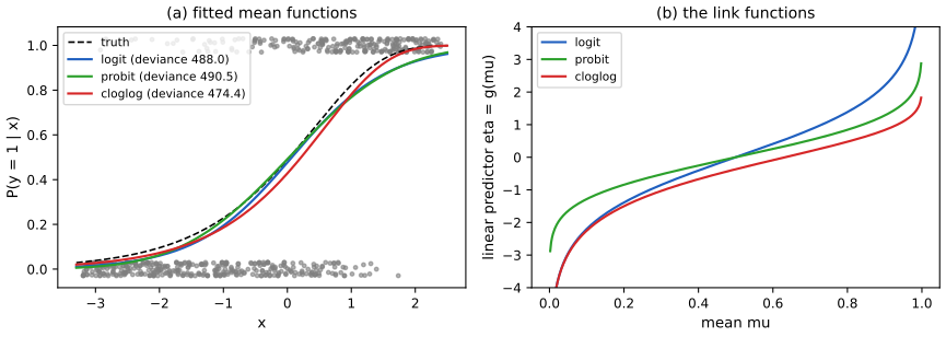
pp. 417–418 The canonical link satisfies \(\theta=\ell(\mu)\) for the natural parameter \(\theta\), so that \(\theta=\ell(\ell^{-1}(\eta))=\eta\) (12.23): the linear score is the natural parameter. For the Bernoulli this is the log-odds \(\ell(\mu)=\logit(\mu)=\log\frac{\mu}{1-\mu}\) (12.24), whose inverse is the sigmoid. Nothing forces this choice; any strictly monotone \(\ell\) with an inverse of the right range gives a valid model \(\mu_n=\ell^{-1}(\bm w^\T\bm x_n)\). Two further links are common for binary responses.
The probit link \(\eta=\Phi^{-1}(\mu)\) (12.25), with \(\Phi\) the standard normal CDF, and the complementary log-log link \[ \eta=\ell(\mu)=\log(-\log(1-\mu)),\qquad\mu=1-\exp(-e^{\eta}). \tag{12.26} \] The latter has a Poisson origin. Let \(E\) be the number of events in a window, Poisson with rate \(\lambda\), and \(y=\mathbb 1\{E\ge1\}\). Then \(p(y=0)=1-\mu=p(E=0)=e^{-\lambda}\) (12.27), so \(\lambda=-\log(1-\mu)\); making the rate positive through a log link, \(\lambda=e^{\eta}\), gives \(\eta=\log\lambda=\log(-\log(1-\mu))\) (12.28). Unlike the logit and probit, it is asymmetric: \(\mu\to1\) double-exponentially fast but \(\mu\to0\) only exponentially fast in \(\eta\).
Result 12.1 (links as latent-threshold models) Section 12.3, supplementary
Let \(y=\mathbb 1\{\eta+\varepsilon>0\}\) where \(\varepsilon\) is independent noise with continuous CDF \(F\). If \(F\) is symmetric about 0, then \(\Pr(y=1)=F(\eta)\). Hence a logistic \(\varepsilon\) gives the logit link, a standard normal \(\varepsilon\) the probit link, and a standard Gumbel \(\varepsilon\) (CDF \(e^{-e^{-t}}\)) gives the complementary log-log link \(\mu=1-\exp(-e^{\eta})\).
Proof
\(\Pr(y=1)=\Pr(\varepsilon>-\eta)=1-F(-\eta)\). If \(F\) is symmetric, \(1-F(-\eta)=F(\eta)\); the logistic CDF is \(\sigma\) and the normal CDF is \(\Phi\). For the Gumbel, which is not symmetric, \(1-F(-\eta)=1-\exp(-e^{\eta})\), which is (12.26). \(\square\) (I confirmed the Gumbel case by simulation.)
The consequence is practical: the logit and probit inverse links are both S-shaped and symmetric, and differ mainly in the tails; the probit coefficients are about \(1.6\)–\(1.8\) times smaller than the logit ones for the same fitted curve because the normal has standard deviation 1 against \(\pi/\sqrt3\approx1.81\) for the logistic. Only the complementary log-log is asymmetric.
See also (companion): Bayesian and Probabilistic ML, Section 4.3.5 (probit regression); ISL, Section 4.6.3 for the link functions in greater generality.
12.4 Maximum likelihood estimation
pp. 418–419 With the canonical link, the negative log likelihood of \(N\) independent observations is, up to terms free of \(\bm w\), \[ \operatorname{NLL}(\bm w)=-\log p(\mathcal D\given\bm w)=-\frac1{\sigma^2}\sum_{n=1}^N\ell_n,\qquad\ell_n\triangleq\eta_ny_n-A(\eta_n). \tag{12.29, 12.30} \] (The book writes the per-observation term as \(\ell_n\), the same letter as the link function; I keep its notation.) Take \(\sigma^2=1\) for now, as the book does. The gradient of one term follows from the chain rule: \[ \bm g_n=\frac{\partial\ell_n}{\partial\bm w}=\frac{\partial\ell_n}{\partial\eta_n}\frac{\partial\eta_n}{\partial\bm w}=(y_n-A'(\eta_n))\,\bm x_n=(y_n-\mu_n)\,\bm x_n, \tag{12.31} \] where \(\mu_n=f(\bm w^\T\bm x_n)\) and \(f=A'\) is the mean function: for logistic regression \(f=\sigma\) and (12.31) is the familiar \(\bm X^\T(\bm y-\bm\mu)\) of Equation (10.21) of the book. Differentiating again, \[ \frac{\partial\bm g_n}{\partial\bm w^\T}=-f'(\eta_n)\,\bm x_n\bm x_n^\T,\qquad\bm H=\frac{\partial^2}{\partial\bm w\,\partial\bm w^\T}\operatorname{NLL}(\bm w)=\sum_{n=1}^Nf'(\eta_n)\,\bm x_n\bm x_n^\T=\bm X^\T\bm S\bm X,\ \ \bm S=\diag\big(f'(\eta_n)\big), \tag{12.32--12.34} \] with \(f'=A''>0\). For the logistic case \(f'=\sigma(1-\sigma)\), recovering (10.23). Since \(\bm v^\T\bm H\bm v=\sum_nf'(\eta_n)(\bm v^\T\bm x_n)^2\ge0\), the NLL is convex, and strictly convex when the \(\bm x_n\) span \(\R^D\) (gap 12.3). With a general dispersion \(\sigma^2\), both the gradient and the Hessian carry a factor \(1/\sigma^2\), which does not move the minimiser. A gradient-based solver (batch or stochastic gradient descent, Newton, L-BFGS) can then be used exactly as for logistic regression.
Filling the gap 12.3: the gradient and Hessian for a general link, observed against expected information, and the exact condition for convexity pp. 418–419, (12.31)–(12.34)
Derivation
Canonical link, with dispersion. The \(n\)-th term of the NLL is \(-(y_n\eta_n-A(\eta_n))/\phi\) plus a constant; \(\partial\eta_n/\partial\bm w=\bm x_n\), so \[ \nabla\operatorname{NLL}=-\frac1\phi\sum_n(y_n-A'(\eta_n))\bm x_n=-\frac1\phi\bm X^\T(\bm y-\bm\mu) \], and \(\nabla^2\operatorname{NLL}=\frac1\phi\bm X^\T\diag(A''(\eta_n))\bm X\). Because \(A''=\var[y]/\phi\ge0\) (gap 12.1) the Hessian is positive semi-definite for every \(\bm w\) and every data set. For all \(\bm v\), \(\bm v^\T\bm H\bm v=\frac1\phi\sum_nA''(\eta_n)(\bm x_n^\T\bm v)^2\) vanishes iff \(\bm x_n^\T\bm v=0\) for every \(n\) (when all \(A''(\eta_n)>0\)), i.e. iff \(\bm X\bm v=0\). So the Hessian is positive definite exactly when \(\bm X\) has full column rank \(D\). The book's argument "\(f'(\eta_n)>0\), hence positive definite" is incomplete without this rank condition (and its condition "\(f(\eta_n)>0\)" should read \(f'(\eta_n)>0\)). With a rank-deficient \(\bm X\), the NLL is convex but flat along \(\ker\bm X\), and the MLE is not unique. (A quick check: duplicating a feature column makes the Hessian singular, which I verified numerically.) A convex function with a positive definite Hessian everywhere is strictly convex, so there is at most one minimiser; existence is a separate matter, see gap 12.4.
General link. Let \(V(\mu)=A''((A')^{-1}(\mu))\) and let \(\theta_n=(A')^{-1}(\mu_n)\) be the natural parameter, with \(\mu_n=\ell^{-1}(\eta_n)\), \(\eta_n=\bm w^\T\bm x_n\). The log likelihood of one case is \((y\theta-A(\theta))/\phi\). Since \(\d\mu/\d\theta=A''(\theta)=V(\mu)\), \(\d\theta/\d\mu=1/V(\mu)\), so \[ \frac{\partial\log p}{\partial\mu}=\frac{y-\mu}{\phi V(\mu)},\qquad\bm s_n\triangleq\frac{\partial\log p}{\partial\bm w}=\frac{y_n-\mu_n}{\phi V(\mu_n)}\frac{\d\mu_n}{\d\eta_n}\bm x_n=(y_n-\mu_n)\,q_n\bm x_n,\quad q_n\triangleq\frac{\d\mu_n/\d\eta_n}{\phi V(\mu_n)}. \] For the canonical link \(\d\mu/\d\eta=A''=V\), so \(q_n=1/\phi\) and \(\bm s_n=(y_n-\mu_n)\bm x_n/\phi\), as above. In general, differentiating \(\bm s_n\) with respect to \(\bm w\), \[ -\frac{\partial\bm s_n}{\partial\bm w^\T}=\Big[\underbrace{\frac{(\d\mu_n/\d\eta_n)^2}{\phi V(\mu_n)}}_{W_n}-(y_n-\mu_n)\frac{\d q_n}{\d\eta_n}\Big]\bm x_n\bm x_n^\T. \] This observed information depends on \(y_n\) through the second term, which vanishes identically for the canonical link (\(q_n\) is constant) and in general only vanishes in expectation, since \(\E[y_n-\mu_n]=0\). The expected information \(\bm I(\bm w)=\E[-\nabla^2\log p]=\bm X^\T\bm W\bm X\) with \(\bm W=\diag(W_n)\) is therefore positive semi-definite for every link, and it equals the covariance of the score, \[ \E[\bm s\bm s^\T]=\sum_n\E[(y_n-\mu_n)^2]q_n^2\bm x_n\bm x_n^\T=\sum_n\phi V(\mu_n)q_n^2\bm x_n\bm x_n^\T=\sum_nW_n\bm x_n\bm x_n^\T \], using \(\var[y_n]=\phi V(\mu_n)\). I checked this identity by simulation for the complementary log-log link, and that for the logit link the observed Hessian does not depend on \(y\), while for the complementary log-log link it does. Consequence: for a non-canonical link the observed Hessian need not be positive semi-definite, so convexity of the NLL is not guaranteed in general (it does hold for the binary logit, probit and complementary log-log models); the expected-information (Fisher scoring) iteration below uses the always positive semi-definite \(\bm X^\T\bm W\bm X\). \(\square\)
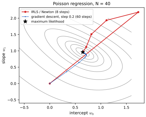
p. 419 Replacing the Hessian by the expected information \(\bm X^\T\bm W\bm X\) gives Fisher scoring, which for the canonical link is Newton's method. It can be written as a sequence of weighted least squares problems, the iteratively reweighted least squares (IRLS) algorithm, which is how GLMs are fitted in most statistical software.
Algorithm (IRLS / Fisher scoring) after (12.34); not numbered in the book
Start from \(\bm w^{(0)}\). Repeat until the change in \(\bm w\) is below a tolerance: with \(\eta_n=\bm x_n^\T\bm w\), \(\mu_n=\ell^{-1}(\eta_n)\), \(d_n=\d\mu_n/\d\eta_n\), set
\[ W_n=\frac{d_n^2}{V(\mu_n)},\qquad z_n=\eta_n+\frac{y_n-\mu_n}{d_n},\qquad\bm w\leftarrow(\bm X^\T\bm W\bm X)^{-1}\bm X^\T\bm W\bm z. \](Dispersion cancels.) For a canonical link \(d_n=V(\mu_n)=A''(\eta_n)\), so \(W_n=A''(\eta_n)\) and \(z_n-\eta_n=(y_n-\mu_n)/A''(\eta_n)\). For the Gaussian family \(W_n=1\) and one step returns the least squares solution. Python: glm_fit in code/ch12_generalized_linear_models.py, which also accepts sample weights (exposures), an offset and a ridge penalty.
Filling the gap 12.4: IRLS is Newton's method, why it converges fast, and when the MLE exists p. 419 ("fit GLMs ... in a manner similar to logistic regression")
Derivation
IRLS equals Fisher scoring. From gap 12.3, \(\bm s_n=(y_n-\mu_n)q_n\bm x_n\) and \(W_n=d_nq_n\) (the common factor \(1/\phi\) cancels in the update; take \(\phi=1\) below). Then \((y_n-\mu_n)q_n=W_n\,(y_n-\mu_n)/d_n=W_n(z_n-\eta_n)\), so the score of the whole sample is \(\bm X^\T\bm W(\bm z-\bm X\bm w)\). Fisher scoring updates \[ \bm w\leftarrow\bm w+(\bm X^\T\bm W\bm X)^{-1}\bm X^\T\bm W(\bm z-\bm X\bm w)=(\bm X^\T\bm W\bm X)^{-1}\bm X^\T\bm W\bm z \]: exactly the weighted least squares solution of regressing the working response \(z_n\) on \(\bm x_n\) with weights \(W_n\). For a canonical link the observed and expected Hessians coincide (gap 12.3), so this is also Newton's method. I confirmed numerically that each IRLS step equals a Newton step with the explicit Hessian, and that the fitted coefficients agree with a standard library for the Gaussian, Bernoulli and Poisson families and for the probit and complementary log-log links.
Local quadratic convergence. Let \(g\) be the gradient of the NLL, \(\bm w^*\) a minimiser with \(\bm H(\bm w^*)\succ0\) and \(\bm H\) Lipschitz near \(\bm w^*\) (true for all three families, since \(A''\) is smooth). Newton's iterate \(\bm w^+=\bm w-\bm H(\bm w)^{-1}g(\bm w)\) has error \[ \bm w^+-\bm w^*=\bm H(\bm w)^{-1}\big[\bm H(\bm w)(\bm w-\bm w^*)-(g(\bm w)-g(\bm w^*))\big] \], and \[ g(\bm w)-g(\bm w^*)=\int_0^1\bm H(\bm w^*+t(\bm w-\bm w^*))\,\d t\,(\bm w-\bm w^*) \]. The bracket is therefore \[ \int_0^1[\bm H(\bm w)-\bm H(\bm w^*+t(\bm w-\bm w^*))]\d t\,(\bm w-\bm w^*) \], of norm at most \(\tfrac12L\|\bm w-\bm w^*\|^2\), and \(\|\bm H(\bm w)^{-1}\|\le2/\lambda_{\min}\) near \(\bm w^*\). So \(\|\bm w^+-\bm w^*\|\le C\|\bm w-\bm w^*\|^2\): the number of correct digits roughly doubles per step once close. Far from \(\bm w^*\) plain Newton may overshoot (the logistic example in the demo zig-zags before converging), so production code adds step halving; gradient descent, by contrast, converges only linearly. The Poisson example in the demo shows both behaviours.
Existence of the MLE. Strict convexity gives uniqueness, not existence. Bernoulli, separation: if some \(\bm v\) has \((2y_n-1)\bm v^\T\bm x_n>0\) for every \(n\) (the classes are linearly separable), then \(\operatorname{NLL}(t\bm v)=\sum_n\log(1+e^{-(2y_n-1)t\bm v^\T\bm x_n})\) decreases strictly to 0 as \(t\to\infty\) while every term is positive: the infimum 0 is not attained and no MLE exists (the example in Exercise 12.5: with \(x=-2,-1,1,2\) and \(y=0,0,1,1\) the NLL along \(w_1=1,5,25\) is \(0.880,\,0.0135,\,2.8\times10^{-11}\)). Poisson, empty cells: if a dummy-coded factor level has no claims in the training data, the corresponding coefficient diverges to \(-\infty\). In both cases a ridge penalty \(\frac\alpha2\|\bm w\|^2\) (leaving the intercept free) makes the objective strongly convex and the minimiser exist and be unique; IRLS then solves \((\bm X^\T\bm W\bm X+\alpha\bm I)\bm w=\bm X^\T\bm W\bm z\) (the penalised score is \(\bm X^\T\bm W(\bm z-\bm X\bm w)-\alpha\bm w\); the code checks it vanishes at the solution). \(\square\)
See also (companion): Bayesian and Probabilistic ML, Section 4.3.3 (IRLS for logistic regression), ESL, Section 4.4.1, ISL, Section 4.3.2.
12.5 Worked example: predicting insurance claims
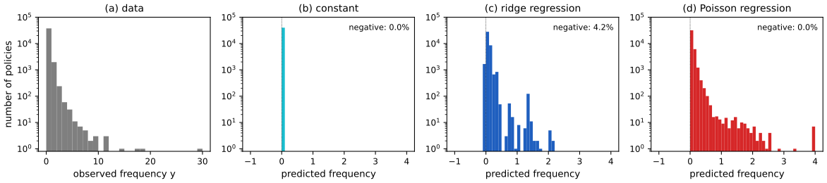
pp. 419–421 The task is to predict the expected number of claims per year for car insurance policies. In the book the data are 678 thousand policies with nine features (driver age, vehicle age, vehicle power, ...), and the target is the claim frequency, the number of claims divided by the exposure (the policy duration in years). The simplest predictor is a constant, the average frequency. A better one is linear regression on engineered features (continuous features binned, categorical ones one-hot encoded; a small \(\ell_2\) penalty makes it a ridge regression). A third is Poisson regression with the same features and the log link. Because the data have a mass at zero (94 percent of policies in the book have no claim) and a long right tail, a Gaussian model fits poorly: it can predict negative frequencies, and it ignores that the variance grows with the mean.
The data used here. The book's data set is not available offline, so the code simulates policies with the same structure (Python simulate_claims): exposures (45% a full year, the rest spread over (0,1)), nine risk factors, a log-linear risk with a strong young-driver effect, claims \(\sim\operatorname{Poi}(\text{exposure}\times\text{rate})\), about 94 percent of policies without a claim and a mean frequency near 9 percent. 160,000 policies, a quarter held out. The three predictors are fitted by exposure-weighted least squares (the weights are the exposures; the book does not say how exposure enters, and the weighting is the right choice for the Poisson likelihood) and by exposure-weighted Poisson maximum likelihood (IRLS from Section 12.4, with the claim frequency as the response and the exposure as a sample weight; this equals a Poisson model for the count with log-exposure as an offset, Exercise 12.3).
How should the three be compared? Mean squared error and mean absolute error reward the ridge model and can even prefer it, because they ignore that a frequency is non-negative and that its variance scales with its mean. The natural measure is the deviance, twice the log-likelihood gap between the saturated model (one free mean per observation, \(\mu^*_i=y_i\)) and the fitted model, \[ D(\bm y,\hat{\bm\mu})=2\sum_i\big(\log p(y_i\given\mu^*_i)-\log p(y_i\given\hat\mu_i)\big), \tag{12.35} \] which for the Poisson model is \[ D(\bm y,\hat{\bm\mu})=2\sum_i\Big[\big(y_i\log y_i-y_i-\log y_i!\big)-\big(y_i\log\hat\mu_i-\hat\mu_i-\log y_i!\big)\Big]=2\sum_i\Big(y_i\log\frac{y_i}{\hat\mu_i}+\hat\mu_i-y_i\Big), \tag{12.36, 12.37} \] with \(0\log0=0\). In the exposure-weighted setting each term is multiplied by the exposure; the code reports the exposure-weighted mean deviance (a negative ridge prediction is floored at 0.001 inside the deviance, since the Poisson deviance needs \(\hat\mu>0\)).
Filling the gap 12.5: why the deviance is the right yardstick: it is a Bregman divergence and a proper scoring rule p. 420, (12.35)–(12.37)
Derivation
Algebra. Subtracting the two Poisson log densities in (12.36), the \(\log y_i!\) terms cancel, leaving \[ y_i\log y_i-y_i-y_i\log\hat\mu_i+\hat\mu_i=y_i\log(y_i/\hat\mu_i)+\hat\mu_i-y_i \], (12.37). It is non-negative: with \(t=y/\hat\mu\), \(y\log(y/\hat\mu)+\hat\mu-y=\hat\mu\,(t\log t-t+1)\ge0\) because \(t\log t\ge t-1\) (convexity of \(t\log t\) at \(t=1\)), with equality iff \(y=\hat\mu\). It is exactly twice the KL divergence between the Poisson with mean \(y\) and the Poisson with mean \(\hat\mu\) (I checked numerically), and for the Gaussian family with \(\sigma^2=1\) the deviance is the residual sum of squares, for the Bernoulli family twice the cross-entropy loss.
General form. For any exponential dispersion family with convex \(A\), the saturated parameter for observation \(y\) is \(\theta^*=(A')^{-1}(y)\) and \[ \tfrac12D_i=\big[y\theta^*-A(\theta^*)\big]-\big[y\hat\theta-A(\hat\theta)\big]=A^*(y)-A^*(\hat\mu)-(A^*)'(\hat\mu)(y-\hat\mu), \] where \(A^*\) is the convex conjugate of \(A\) (so \(A^*(\mu)=\mu\theta-A(\theta)\) with \(\theta=(A')^{-1}(\mu)\), and \((A^*)'(\mu)=\theta\)). This is the Bregman divergence of the convex function \(A^*\) between \(y\) and \(\hat\mu\): it is non-negative and zero iff \(y=\hat\mu\). For the Poisson model \(A^*(\mu)=\mu\log\mu-\mu\).
Proper scoring rule. Let \(y\) have mean \(m_0\) (any distribution), and consider predicting with a constant \(m\). Then \[ \E[\,2A^*(y)-2A^*(m)-2(A^*)'(m)(y-m)\,]=2\E[A^*(y)]-2A^*(m)-2(A^*)'(m)(m_0-m), \] and its derivative in \(m\) is \(-2(A^*)''(m)(m_0-m)\), which has the sign of \(m-m_0\) because \((A^*)''=1/A''>0\). Hence the expected deviance is uniquely minimised at \(m=m_0\): predicting the true mean is optimal, i.e. the deviance is a strictly proper scoring rule for the mean. (Numerically, for \(y\sim\operatorname{Poi}(0.3)\) the expected Poisson deviance is minimised at \(m=0.300\).) Squared error is also proper for the mean (it is the Bregman divergence of \(\mu^2\)), but it is a poor measure of fit for counts because it weights all errors alike whatever the mean. The mean absolute error is not proper for the mean: it is minimised by the median, which is 0 for a Poisson variable with mean 0.3 (confirmed numerically), so for data with 94 percent zeros MAE rewards predictions that are too small. This explains why in the book's Table 12.1, and in mine, differences in MSE and MAE between the models are slight while the deviance separates them. \(\square\)
| Name | MSE | MAE | Deviance | Predicted claims (test) |
|---|---|---|---|---|
| Dummy | 0.239 | 0.160 | 0.494 | 2528 |
| Ridge | 0.221 | 0.150 | 0.431 | 2527 |
| Poisson | 0.207 | 0.149 | 0.419 | 2576 |
Table 12.1 (reproduced on the simulated data; 40,000 test policies, 2588 observed claims). Exposure-weighted test MSE, MAE and mean Poisson deviance of the constant, ridge and Poisson predictors. Poisson regression is best on all three here. In the book's real data the picture is less clear-cut (MSE 0.560 for both ridge and Poisson, MAE 0.177 against 0.186 in favour of ridge, deviance 0.601 against 0.594 in favour of Poisson), which is why the deviance and the calibration plot are the better guides. The last column is the sum over test policies of exposure times prediction. Reproduces Murphy (2022), Table 12.1.
A second diagnostic is the calibration plot: sort the test policies by predicted frequency, split them into groups of equal exposure (ten here), and plot in each group the mean predicted and the mean observed frequency; a calibrated model has the two curves on top of each other.
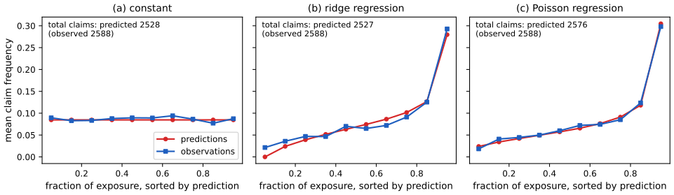
The book also compares the total number of predicted and observed claims on the test set (the ridge model underestimates it, the Poisson model matches it). On the training set this holds exactly for the Poisson model, by a property of the score equations; on new data it holds only up to sampling error (gap 12.6).
Filling the gap 12.6: why the Poisson fit reproduces the total number of claims p. 421
Derivation
For the exposure-weighted Poisson model with an intercept, the score equations at the MLE are \(\sum_nt_n(y_n-\hat\mu_n)\bm x_n=0\), where \(t_n\) is the exposure and \(y_n\) the frequency (gradient (12.31) with sample weights). The first coordinate of \(\bm x_n\) is 1, so \(\sum_nt_ny_n=\sum_nt_n\hat\mu_n\): the total predicted claims equal the total observed claims on the training set. The same holds for every dummy column: for each level of each factor, predicted and observed claims agree in total, because the corresponding score equation is \(\sum_{n\in\text{level}}t_n(y_n-\hat\mu_n)=0\). This is a property of every canonical-link GLM with an intercept; with a non-canonical link the score is weighted by \(q_n\) (gap 12.3) and it fails. For the ridge regression with an unpenalised intercept the normal equations give \(\sum_nt_n(y_n-\hat y_n)=0\) as well, so the training totals agree for it too (the code confirms both). The difference seen on the test set is therefore not a failure of in-sample calibration but a matter of generalisation: the totals can differ through sampling variation (a claim count of 2588 has standard deviation about 51) and through model misfit, which is what the calibration plot reveals decile by decile. In my simulation the test totals are 2527 (ridge) and 2576 (Poisson) against 2588 observed, both within about 1.2 standard deviations: the totals alone do not separate the models, the calibration curve and the deviance do. \(\square\)
See also (companion): ISL, Section 4.6.2 (Poisson regression on the bikeshare data, where the linear model also predicts negative counts).
12.6 Exercises
The book has no exercises for Chapter 12. The five below are my own: each fills a point the chapter leaves open, with a complete solution (hidden). The numbers quoted were confirmed by simulation or direct computation.
Exercise 12.1 (Gamma regression). A positive response has the Gamma density with mean \(\mu\) and shape \(\nu\): \(p(y)=\frac{(\nu/\mu)^\nu}{\Gamma(\nu)}y^{\nu-1}e^{-\nu y/\mu}\). Put it in the form (12.1), find the canonical link, the variance function, and say why the log link is used in practice.
Solution
\[ \log p=\nu\big(-y/\mu-\log\mu\big)+(\nu-1)\log y+\nu\log\nu-\log\Gamma(\nu) \]. With \(\theta=-1/\mu\) (so \(\mu=-1/\theta\), \(\theta<0\)) and \(\phi=1/\nu\): \(-y/\mu=y\theta\) and \(-\log\mu=\log(-\theta)\), so \(\log p=\frac{y\theta-A(\theta)}{\phi}+\log h\) with \(A(\theta)=-\log(-\theta)\). Then \(A'(\theta)=-1/\theta=\mu\) and \(A''(\theta)=1/\theta^2=\mu^2\), so \(\var[y]=\phi\mu^2=\mu^2/\nu\): the standard deviation is proportional to the mean (constant coefficient of variation). The canonical link is \(\theta=-1/\mu\) (the reciprocal link); it forces \(\bm w^\T\bm x<0\) and is rarely used. The log link \(\mu=e^{\bm w^\T\bm x}\) keeps \(\mu>0\) for every \(\bm w\), gives multiplicative effects, and is the common choice for claim amounts, durations and concentrations. Because it is not canonical, IRLS uses the Fisher-scoring weights \(W=d^2/V=\mu^2/\mu^2=1\) with working response \(z=\eta+(y-\mu)/\mu\). Numerically I confirmed \(A'=\mu\), \(A''=\mu^2\) by finite differences and \(\var[y]=\mu^2/\nu\) by simulation. \(\square\)
Exercise 12.2 (latent variables). Simulate \(y=\mathbb 1\{\eta+\varepsilon>0\}\) with \(\varepsilon\) standard Gumbel (CDF \(e^{-e^{-t}}\)) and \(\eta=0.4\); what fraction of ones do you expect, and which link generates it? Which noise gives the probit link?
Solution
By Result 12.1, \(\Pr(y=1)=1-F(-\eta)=1-\exp(-e^{0.4})=1-\exp(-1.4918)=0.7750\): the complementary log-log link. A sample of 600,000 draws gave a fraction within 0.004 of this value. The probit link arises from standard normal noise: \(\Pr(y=1)=\Phi(\eta)\) by symmetry. (A logistic noise gives the logit.) The latent view also shows why the logit and probit coefficients differ by a scale: the logistic distribution has standard deviation \(\pi/\sqrt3\approx1.81\), so \(\bm w_{\text{logit}}\approx1.7\bm w_{\text{probit}}\), as in the fits of Figure 12.S1 and the demo (1.33 against 0.75, a ratio of 1.76). \(\square\)
Exercise 12.3 (exposure and offsets). Policy \(n\) is insured for \(t_n\) years, and the claim count is \(y_n\sim\operatorname{Poi}(t_n\lambda_n)\) with \(\log\lambda_n=\bm w^\T\bm x_n\). (a) Show this is a Poisson GLM with \(\log\mu_n=\log t_n+\bm w^\T\bm x_n\) (an offset) and write the score. (b) Show that the exposure-weighted model for the frequency \(y_n/t_n\) with weights \(t_n\) has the same score. (c) For the intercept-only model, find the MLE and the Newton iteration, and run it for \(t=(0.5,1,2,0.25)\), \(y=(1,0,3,0)\).
Solution
(a) \(\mu_n=t_n\lambda_n=\exp(\log t_n+\bm w^\T\bm x_n)\), so the linear predictor has the fixed extra term \(\log t_n\) (the offset, a covariate with coefficient fixed at 1). The log likelihood is \(\sum_n[y_n(\log t_n+\eta_n)-t_ne^{\eta_n}-\log y_n!]\), with score \(\sum_n(y_n-t_ne^{\eta_n})\bm x_n\). (b) For the frequency \(f_n=y_n/t_n\) with weight \(t_n\) the weighted score (12.31) is \(\sum_nt_n(f_n-e^{\eta_n})\bm x_n=\sum_n(y_n-t_ne^{\eta_n})\bm x_n\): identical, so the two formulations have the same MLE (the likelihoods differ only by terms free of \(\bm w\)); the code uses the second. (c) With only an intercept \(w\), \(\sum_n(y_n-t_ne^w)=0\) gives \(e^{\hat w}=\sum y_n/\sum t_n\) (the total claims per total year of exposure). Newton's step is \(w\leftarrow w+(\sum y_n-\sum t_ne^w)/\sum t_ne^w\). From \(w=0\): \(\sum y=4\), \(\sum t=3.75\), giving \(w=0.0667,\,0.06454078,\,0.06453852,\,\ldots\) and \(e^{\hat w}=4/3.75=1.0667\); the iterate is already at 6 digits after three steps (quadratic convergence). The library fit with offset \(\log t\) gave the same value. \(\square\)
Exercise 12.4 (over-dispersion). A Poisson model forces \(\var[y]=\mu\). Suppose the rate itself varies: \(y\given\lambda\sim\operatorname{Poi}(\lambda)\) with \(\lambda\sim\operatorname{Gamma}(\text{shape }r,\text{ mean }\mu)\). Show that \(\E[y]=\mu\) and \(\var[y]=\mu+\mu^2/r\), and say how the Poisson regression standard errors are affected.
Solution
By the laws of total expectation and variance, \(\E[y]=\E[\lambda]=\mu\) and \[ \var[y]=\E[\var(y\given\lambda)]+\var[\E(y\given\lambda)]=\E[\lambda]+\var[\lambda]=\mu+\mu^2/r \], since a Gamma with shape \(r\) and mean \(\mu\) has variance \(\mu^2/r\). The marginal of \(y\) is the negative binomial distribution. A simulation with \(r=2.5\), \(\mu=1.3\) (500,000 draws) gave mean 1.302 and variance 1.986 against the theoretical 1.976. The variance is larger than the mean (over-dispersion), and the ratio \(\var/\mu=1+\mu/r\) grows with \(\mu\). If one fits a Poisson GLM to over-dispersed data, the point estimates of \(\bm w\) are still consistent (the score equations are unbiased as long as the mean is right) but the usual standard errors, which assume \(\var=\mu\), are too small; remedies are a dispersion parameter estimated from the Pearson residuals (quasi-likelihood), robust (sandwich) standard errors, or the negative binomial model. \(\square\)
Exercise 12.5 (separation). For logistic regression with data \(x=(-2,-1,1,2)\), \(y=(0,0,1,1)\) and \(\eta=w_0+w_1x\), show that no MLE exists, compute the NLL along \((0,w_1)\) for \(w_1=1,5,25\), and find the ridge solution with penalty \(\frac{1}{2}w_1^2\) (intercept unpenalised).
Solution
The data are separated by \(v=(0,1)\): \((2y_n-1)v^\T\bm x_n=2,1,1,2>0\). By gap 12.4, \[ \operatorname{NLL}(0,t)=\sum_n\log(1+e^{-(2y_n-1)tx_n})=2\log(1+e^{-2t})+2\log(1+e^{-t}) \] decreases strictly to 0 and is never 0, so no minimiser exists. Numerically, at \(t=1\) it equals \[ 2\log(1+e^{-2})+2\log(1+e^{-1})=0.2538+0.6266=0.8804, \] at \(t=5\) it is \(0.0135\) and at \(t=25\) it is \(2.8\times10^{-11}\). With the penalty \(\frac12w_1^2\), the objective \(\operatorname{NLL}+\frac12w_1^2\) is strongly convex; by symmetry \(w_0=0\), and solving \(\sum_n(y_n-\mu_n)x_n=w_1\) by IRLS gives \(w_1=1.0066\) (a finite, stable answer). Without the penalty the IRLS iteration would let \(w_1\) grow without bound while the fitted probabilities approach 0 and 1. \(\square\)
Demonstrations
| Page | What it shows | In the notes |
|---|---|---|
| IRLS against gradient descent | Gaussian, Bernoulli and Poisson GLMs with one input; the fitted mean after k iterations and the path over the contours of the negative log likelihood. Presets: 1 Poisson by IRLS; 2 Gaussian in one step; 3 logistic from far away; 4 gradient descent; 5 an unstable step. | 12.4, gap 12.3, gap 12.4 |
| Link functions for binary data | Logit, probit and complementary log-log fitted to the same data; deviances, AIC, tail behaviour on log scales. Presets: 1 all points; 2 60 points; 3 probit against logit; 4 lower tail; 5 upper tail. | 12.3, Result 12.1 |
| Ridge against Poisson regression on claims | Constant, ridge and Poisson predictors of claim frequency on simulated policies; MSE, MAE, deviance, totals, calibration. Presets: 1 Poisson; 2 ridge; 3 constant; 4 little data; 5 one factor. | 12.5, gap 12.5, gap 12.6 |
The Python code that produces every figure of this page is code/ch12_generalized_linear_models.py (see the code index). Companion demos: logistic regression, ridge regression and cross-validation (Chapter 4 of this course).
Notes on the book
Points where the book is imprecise or wrong
- (12.2) and the definition of the mean function. The equation \(\E[y_n]=A'(\eta_n)\triangleq\ell^{-1}(\eta_n)\) is true only for the canonical link, where the natural parameter equals the linear score. The introduction writes the model as if this were always so and Section 12.3 only then relaxes it. For a general link \(\mu=\ell^{-1}(\eta)\) and \(A'(\theta)=\mu\) hold with different arguments (Filling the gap 12.3).
- (12.34) and positive definiteness. The Hessian \(\sum_nf'(\eta_n)\bm x_n\bm x_n^\T\) is positive definite only if \(\bm X\) has full column rank; \(f'(\eta_n)>0\) alone gives positive semi-definiteness. The accompanying condition "\(f(\eta_n)>0\)" should be \(f'(\eta_n)>0\). Uniqueness of the MLE needs the rank condition, and existence is a separate issue (separation in the Bernoulli model, empty cells in the Poisson model; Filling the gap 12.4).
- (12.29)–(12.34) assume \(\sigma^2=1\). The text says so; with a general dispersion the NLL, gradient and Hessian all carry the factor \(1/\sigma^2\). Not an error, but the equations as printed do not follow (12.1) when \(\sigma^2\ne1\).
- Section 12.5, "the Poisson model predicts the total number of claims." The book contrasts the test-set totals (10,693 for the ridge model, 11,930 for the Poisson model, against 11,935 observed). Both models reproduce the training total exactly when they have an unpenalised intercept (Filling the gap 12.6); a test-set difference reflects generalisation and sampling variation, so by itself it is weak evidence for one model. The calibration curve is the better diagnostic.
- (12.37) and exposure. The formula is stated for unweighted observations, and the text does not say how the exposure of a policy enters the fit or the metrics. For a frequency target the Poisson likelihood is only right if each term is weighted by the exposure (equivalently, a count model with a log-exposure offset, Exercise 12.3); the deviance is then a weighted sum, as computed here.
References
- Murphy, K. P. (2022). Probabilistic Machine Learning: An Introduction. MIT Press, Cambridge, MA. Chapter 12, pp. 415–421. probml.github.io/pml-book/book1.html.
- McCullagh, P. and Nelder, J. A. (1989). Generalized Linear Models, 2nd edition. Chapman and Hall, London.
- Nelder, J. A. and Wedderburn, R. W. M. (1972). Generalized linear models. Journal of the Royal Statistical Society, Series A, 135(3), 370–384.
- Green, P. J. (1984). Iteratively reweighted least squares for maximum likelihood estimation, and some robust and resistant alternatives. Journal of the Royal Statistical Society, Series B, 46(2), 149–192.
- Bregman, L. M. (1967). The relaxation method of finding the common point of convex sets and its application to the solution of problems in convex programming. USSR Computational Mathematics and Mathematical Physics, 7(3), 200–217.
- Gneiting, T. and Raftery, A. E. (2007). Strictly proper scoring rules, prediction, and estimation. Journal of the American Statistical Association, 102(477), 359–378.
- Albert, A. and Anderson, J. A. (1984). On the existence of maximum likelihood estimates in logistic regression models. Biometrika, 71(1), 1–10.
- Bishop, C. M. (2006). Pattern Recognition and Machine Learning. Springer, New York.
- Hastie, T., Tibshirani, R. and Friedman, J. (2009). The Elements of Statistical Learning, 2nd edition. Springer, New York.
The numerical statements in the text (mean and variance formulas, the GLM forms of the densities, gradients and Hessians against finite differences, the IRLS and library fits, the deviance identities, the Gumbel latent-variable fraction, the separation example, the over-dispersion example and the figures of the simulated claims data) were confirmed numerically.