Linear Models for Classification
Classification assigns an input to one of a finite number of classes. This chapter studies models whose decision boundaries are hyperplanes in a (possibly fixed non-linear) feature space. It first fits such boundaries directly (least squares, Fisher's discriminant, the perceptron), then derives them from generative class models (a Gaussian or exponential-family density per class, which makes the posterior a logistic sigmoid or softmax of a linear function), then fits the posterior directly by logistic regression with an iterative reweighted least squares algorithm. The last two sections introduce the Laplace approximation and use it to make logistic regression Bayesian. Every step the book leaves to the reader is written out below.
Ch. 1 Introduction Ch. 2 Probability distributions Ch. 3 Linear regression Ch. 4 Linear classification Ch. 5 Neural networks Ch. 6 Kernel methods Ch. 7 Sparse kernel machines Ch. 8 Graphical models Ch. 9 Mixture models and EM Ch. 10 Approximate inference Ch. 11 Sampling methods Ch. 12 Continuous latent variables Ch. 13 Sequential data Ch. 14 Combining models
How to read these notes
They follow the book. Sections carry Bishop's numbers (4.1, 4.3.3, ...) and every displayed equation that appears in the book carries the book's own equation number, e.g. (4.91), so you can read these notes next to the book. Equations without a number are steps that the book skips.
Filling the gaps. Wherever the book says that a result "is easily verified", follows "after some straightforward algebra", or is left as an exercise, an orange Filling the gap box or a proof gives the full argument. Proofs and derivations start hidden: open one with its bar, or use the button below.
Figures and demonstrations. The numerical figures of the chapter are reproduced from scratch by the Python code; the geometry sketch is redrawn. The ▶ Demo boxes open an interactive demonstration already set to the case being discussed. Standard identities (matrix calculus, Gaussian marginals and conditionals, the exponential family, Lagrange multipliers, the Rayleigh quotient) are proved once in the mathematical toolkit.
Main reference
C. M. Bishop, Pattern Recognition and Machine Learning, Springer (2006), Chapter 4, pages 179–224. Section, equation, figure and exercise numbers below refer to this book. Further reading is listed in the references.
The explanations, derivations and code are my own; equations are cited by their numbers in the book.
The chapter at a glance
- 4.1 A linear discriminant \(y(\mathbf{x})=\mathbf{w}^\T\mathbf{x}+w_0\) has a hyperplane as decision surface; with \(K\) classes the single \(K\)-function form has convex decision regions. Least squares has a closed form but is not robust and can mask a class entirely. Fisher's criterion (large between-class, small within-class scatter) gives a direction by a generalised eigenproblem and coincides with least squares for suitable targets. The perceptron updates on mistakes and, for separable data, stops after at most \(R^2/\gamma^2\) of them (Result 4.7).
- 4.2 Bayes' theorem turns class-conditional densities into a posterior \(\sigma(a)\) or softmax. Gaussians with a shared covariance, discrete naive-Bayes features and the exponential family with a shared scale all make \(a\) linear in \(\mathbf{x}\). Maximum likelihood gives class fractions, class means and a pooled covariance.
- 4.3 Fit \(p(\mathcal{C}_k\given\bm\phi)\) directly: logistic regression has \(M\) parameters instead of \(M(M+5)/2+1\). The gradient is \(\sum_n(y_n-t_n)\bm\phi_n\), the Hessian \(\bm\Phi^\T\mathbf{R}\bm\Phi\) is positive semi-definite (definite for full-rank \(\bm\Phi\)), Newton-Raphson becomes IRLS, and on separable data the weights diverge. Softmax, probit and canonical link functions follow the same pattern.
- 4.4–4.5 The Laplace approximation replaces a density by a Gaussian at its mode; applied to the evidence it gives the Occam factor and BIC, applied to the weight posterior of logistic regression it gives a Gaussian \(q(\mathbf{w})\), and the probit trick turns the intractable predictive integral into \(\sigma(\kappa(\sigma_a^2)\mu_a)\).
Notation. Inputs \(\mathbf{x}\in\R^D\), features \(\bm\phi=\bm\phi(\mathbf{x})\in\R^M\) (with \(\phi_0=1\)), \(N\) training pairs \((\mathbf{x}_n,\mathbf{t}_n)\), \(N_k\) points in class \(\mathcal{C}_k\), design matrix \(\bm\Phi\in\R^{N\times M}\) with rows \(\bm\phi_n^\T\). Two-class targets are \(t\in\{0,1\}\) for probabilistic models and \(t\in\{-1,+1\}\) for the perceptron; \(K\)-class targets use the 1-of-\(K\) code. \(\sigma(a)=1/(1+e^{-a})\) is the logistic sigmoid and \(\Phi(a)\)
Prerequisites. Linear regression and the pseudo-inverse (Chapter 3), Gaussian marginals and conditionals, maximum likelihood for a Gaussian and the exponential family (Chapter 2 and the toolkit), decision theory (Chapter 1), Lagrange multipliers and matrix calculus (toolkit, toolkit).
Printings. The text used here is a corrected printing in which some of the book's errata are already applied. Where Bishop's errata list corrects an equation of this chapter, the notes give the corrected form and a short Erratum note. A few places where the extracted equation lost a factor in printing (the \(\tfrac12\) in (4.127), (4.131), (4.139)) are given in their correct form without comment.
4.1 Discriminant functions
pp. 181–196 A discriminant is a function that maps an input straight to a class label, with no probabilities in between. The word "linear" says that the surfaces separating the classes are hyperplanes; the chapter starts with the geometry of such surfaces and then meets three ways of choosing them: least squares, Fisher's criterion and the perceptron.
Definition 4.1 (decision regions, linear separability) pp. 179–181
A classifier splits the input space into decision regions \(\mathcal{R}_k\) (all inputs assigned to \(\mathcal{C}_k\)); their common boundaries are decision boundaries or decision surfaces. A data set is linearly separable if some linear decision surface classifies every training point correctly. In the two-class case with feature vectors \(\bm\phi_n\) this means that there is \(\mathbf{w}\) with \(\mathbf{w}^\T\bm\phi_n>0\) for the points of \(\mathcal{C}_1\) and \(\mathbf{w}^\T\bm\phi_n<0\) for those of \(\mathcal{C}_2\), the bias being absorbed in \(\phi_0=1\).
4.1.1 Two classes
pp. 181–182 The simplest discriminant is an affine function of the input,
\[ y(\mathbf{x})=\mathbf{w}^\T\mathbf{x}+w_0, \tag{4.4} \]with the rule "assign \(\mathbf{x}\) to \(\mathcal{C}_1\) if \(y(\mathbf{x})\ge0\), otherwise to \(\mathcal{C}_2\)". The weight vector \(\mathbf{w}\) is a normal to the decision surface \(y(\mathbf{x})=0\) and \(w_0\) is the bias (not the bias of statistics; \(-w_0\) is a threshold).
Result 4.1 (geometry of a linear discriminant) pp. 181–182, (4.5)–(4.8), Figure 4.1
(a) \(\mathbf{w}\) is orthogonal to every vector lying in the decision surface. (b) The signed perpendicular distance from the origin to the surface is
\[ \frac{\mathbf{w}^\T\mathbf{x}}{\|\mathbf{w}\|}=-\frac{w_0}{\|\mathbf{w}\|}\quad(\mathbf{x}\text{ on the surface}). \tag{4.5} \](c) The signed perpendicular distance of any point \(\mathbf{x}\) from the surface is
\[ r=\frac{y(\mathbf{x})}{\|\mathbf{w}\|}. \tag{4.7} \](d) With \(\tilde{\mathbf{w}}=(w_0,\mathbf{w})\) and \(\tilde{\mathbf{x}}=(1,\mathbf{x})\), \(y(\mathbf{x})\)
Proof
(a) If \(\mathbf{x}_A,\mathbf{x}_B\) lie on the surface then \(y(\mathbf{x}_A)=y(\mathbf{x}_B)=0\), so \(\mathbf{w}^\T(\mathbf{x}_A-\mathbf{x}_B)=0\); the differences of surface points span the surface's tangent space.
(b) For \(\mathbf{x}\) on the surface, \(\mathbf{w}^\T\mathbf{x}=-w_0\), and the component of \(\mathbf{x}\) along the unit normal \(\mathbf{w}/\|\mathbf{w}\|\) is \(\mathbf{w}^\T\mathbf{x}/\|\mathbf{w}\|\) (all surface points have the same component, so this is the distance from the origin to the hyperplane).
(c) Let \(\mathbf{x}_\perp\) be the orthogonal projection of \(\mathbf{x}\) onto the surface, so that \(\mathbf{x}\)
(d) is direct substitution. ∎
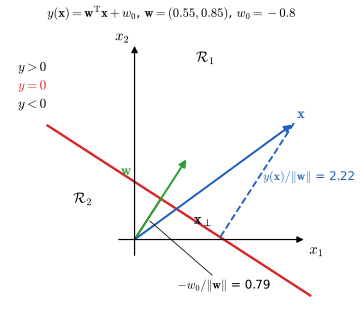
fig4_1. Download: PDF · SVG4.1.2 Multiple classes
pp. 182–184 With \(K>2\) classes one is tempted to combine two-class discriminants. One-versus-the-rest trains \(K-1\) classifiers, the \(k\)th separating \(\mathcal{C}_k\) from the union of the others; one-versus-one trains \(K(K-1)/2\) classifiers, one per pair, and takes a majority vote. Both leave ambiguous regions (Figure 4.2 of the book, a schematic with three classes in the plane):
- One-versus-the-rest. Take two classifiers, "\(\mathcal{C}_1\) or not" and "\(\mathcal{C}_2\) or not". A point on the \(\mathcal{C}_1\) side of the first and the \(\mathcal{C}_2\) side of the second is claimed by both; a point on the "not" side of both is claimed by neither.
- One-versus-one. With three classes the three pairwise lines can form a triangle in which the votes are cyclic, \(\mathcal{C}_1\) beats \(\mathcal{C}_2\) beats \(\mathcal{C}_3\) beats \(\mathcal{C}_1\), so there is no majority.
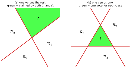
fig4_2. Download: PDF · SVGThe remedy is a single \(K\)-class discriminant of \(K\) linear functions,
\[ y_k(\mathbf{x})=\mathbf{w}_k^\T\mathbf{x}+w_{k0}, \tag{4.9} \]with the rule: assign \(\mathbf{x}\) to \(\mathcal{C}_k\) if \(y_k(\mathbf{x})>y_j(\mathbf{x})\) for all \(j\ne k\). Every point has one largest value (ties occur only on the boundaries), so there are no ambiguous regions. The boundary between \(\mathcal{C}_k\) and \(\mathcal{C}_j\) is where the two functions are equal, which is again a hyperplane,
\[ (\mathbf{w}_k-\mathbf{w}_j)^\T\mathbf{x}+(w_{k0}-w_{j0})=0, \tag{4.10} \]with the geometry of Result 4.1 (normal \(\mathbf{w}_k-\mathbf{w}_j\)).
Result 4.2 (decision regions of a linear \(K\)-class discriminant are convex) pp. 183–184, (4.11), (4.12), Figure 4.3
Every region \(\mathcal{R}_k\)
Proof
Let \(\mathbf{x}_A,\mathbf{x}_B\in\mathcal{R}_k\) and \(\hat{\mathbf{x}}\)
The regions are also open polyhedra: each is an intersection of the \(K-1\) open half-spaces \(\{y_k>y_j\}\), \(j\ne k\). Convexity is what a non-linear discriminant gives up (for instance the quadratic discriminant of Section 4.2.1).
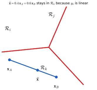
fig4_3. Download: PDF · SVGFor \(K=2\) the one-function form (4.4) and the two-function form (4.9) are equivalent: take \(y=y_1-y_2\), \(\mathbf{w}=\mathbf{w}_1-\mathbf{w}_2\), \(w_0=w_{10}-w_{20}\).
4.1.3 Least squares for classification
pp. 184–186 Chapter 3 gave a closed-form solution for linear models under a sum-of-squares error, so it is tempting to reuse it. Code the class of \(\mathbf{x}_n\) by the 1-of-\(K\) target \(\mathbf{t}_n\) and give each class its own linear model, collected as
\[ \mathbf{y}(\mathbf{x})=\widetilde{\mathbf{W}}^\T\widetilde{\mathbf{x}}, \tag{4.14} \]where the \(k\)th column of \(\widetilde{\mathbf{W}}\) is \(\tilde{\mathbf{w}}_k=(w_{k0},\mathbf{w}_k^\T)^\T\) (so (4.14) stacks the \(K\) functions (4.13)), and assign \(\mathbf{x}\) to the class with the largest \(y_k\). One motivation is that least squares estimates the conditional mean \(\mathbb{E}[\mathbf{t}\given\mathbf{x}]\), and for a 1-of-\(K\) code that is the vector of posterior class probabilities.
Filling the gap 4.1: the least-squares solution and its pseudo-inverse form p. 185, (4.15)–(4.17)
The book "sets the derivative to zero". Let \(\widetilde{\mathbf{X}}\) be the \(N\times(D+1)\) matrix with rows \(\tilde{\mathbf{x}}_n^\T\) and \(\mathbf{T}\) the \(N\times K\) matrix with rows \(\mathbf{t}_n^\T\). The error is
\[ E_D(\widetilde{\mathbf{W}})=\tfrac12\operatorname{Tr}\{(\widetilde{\mathbf{X}}\widetilde{\mathbf{W}}-\mathbf{T})^\T(\widetilde{\mathbf{X}}\widetilde{\mathbf{W}}-\mathbf{T})\}. \tag{4.15} \]Derivation
Write \(\mathbf{R}\)
If \(\widetilde{\mathbf{X}}^\T\widetilde{\mathbf{X}}\) is invertible (full column rank, which needs \(N\ge D+1\)),
\[ \widetilde{\mathbf{W}}=(\widetilde{\mathbf{X}}^\T\widetilde{\mathbf{X}})^{-1}\widetilde{\mathbf{X}}^\T\mathbf{T}=\widetilde{\mathbf{X}}^\dagger\mathbf{T}, \tag{4.16} \]with \(\widetilde{\mathbf{X}}^\dagger\)
Result 4.3 (linear constraints on the targets are inherited by the prediction) p. 185, (4.18), (4.19); Exercises 4.2, 4.3
If every target satisfies \(\mathbf{a}^\T\mathbf{t}_n+b=0\) (4.18), then the least-squares prediction satisfies \(\mathbf{a}^\T\mathbf{y}(\mathbf{x})+b=0\) for every \(\mathbf{x}\) (4.19), provided the model contains a constant basis function. The same holds for several constraints at once. In particular with a 1-of-\(K\) code (\(\mathbf{a}=\mathbf{1}\), \(b=-1\)) the outputs sum to one.
Proof
The constraint says \(\mathbf{T}\mathbf{a}+b\mathbf{1}=\mathbf{0}\) (a vector of length \(N\)). With (4.16)–(4.17),
\[ \mathbf{a}^\T\mathbf{y}(\mathbf{x})=\mathbf{a}^\T\mathbf{T}^\T\widetilde{\mathbf{X}}(\widetilde{\mathbf{X}}^\T\widetilde{\mathbf{X}})^{-1}\tilde{\mathbf{x}}=(\mathbf{T}\mathbf{a})^\T\widetilde{\mathbf{X}}(\widetilde{\mathbf{X}}^\T\widetilde{\mathbf{X}})^{-1}\tilde{\mathbf{x}}=-b\,\mathbf{1}^\T\widetilde{\mathbf{X}}(\widetilde{\mathbf{X}}^\T\widetilde{\mathbf{X}})^{-1}\tilde{\mathbf{x}}. \]Because the first column of \(\widetilde{\mathbf{X}}\) is all ones, \(\mathbf{1}=\widetilde{\mathbf{X}}\mathbf{e}_0\) with \(\mathbf{e}_0=(1,0,\dots,0)^\T\). Then \(\mathbf{1}^\T\widetilde{\mathbf{X}}(\widetilde{\mathbf{X}}^\T\widetilde{\mathbf{X}})^{-1}\)
The sum-to-one property is not enough for probabilities: nothing keeps the outputs inside \((0,1)\), and a linear model must leave that interval somewhere.
Where least squares fails
- Not robust. A point far on the correct side of the boundary is "too correct": its residual is large, so it drags the fit (Figure 4.4, right). Section 7.1.2 meets error functions without this flaw.
- Masking. With three or more classes whole classes can disappear (Figure 4.5, left). A closed-form example: put the same number of points at the three positions \(x=-2,\,0,\,2\) on a line, one class per position. Least squares on each 1-of-3 column gives (computed exactly, one point per class) \(y_1=\tfrac13-\tfrac14x\), \(y_2=\tfrac13\), \(y_3=\tfrac13+\tfrac14x\): the middle class has a flat line that never strictly exceeds the maximum of the other two (all three are equal at \(x=0\)), so the middle class owns no region at all, although it is trivially separable by two thresholds.
- Wrong noise model. Least squares is maximum likelihood for Gaussian conditional targets (Chapter 3), and binary 1-of-\(K\) vectors are anything but Gaussian. The probabilistic models below use a likelihood that matches the data.
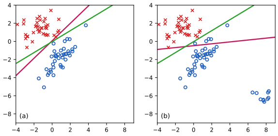
fig4_4. Download: PDF · SVG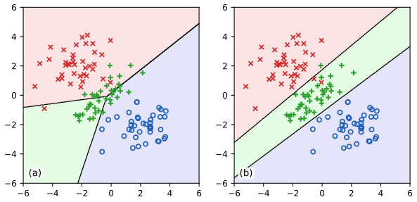
fig4_5. Download: PDF · SVG4.1.4 Fisher's linear discriminant
pp. 186–189 A linear classifier can be seen as a dimension reduction: project \(\mathbf{x}\in\R^D\) to one number,
\[ y=\mathbf{w}^\T\mathbf{x}, \tag{4.20} \]and classify by a threshold on \(y\) (the earlier rule with \(y_0=-w_0\)). Let \(N_1,N_2\) be the class sizes, with class means
\[ \mathbf{m}_1=\frac1{N_1}\sum_{n\in\mathcal{C}_1}\mathbf{x}_n,\qquad \mathbf{m}_2=\frac1{N_2}\sum_{n\in\mathcal{C}_2}\mathbf{x}_n. \tag{4.21} \]The first idea is to separate the projected means: maximise \(m_2-m_1=\mathbf{w}^\T(\mathbf{m}_2-\mathbf{m}_1)\) (4.22), with \(m_k=\mathbf{w}^\T\mathbf{m}_k\) (4.23). This is unbounded in \(\|\mathbf{w}\|\), so constrain \(\mathbf{w}^\T\mathbf{w}=1\).
Filling the gap 4.2: the constrained maximisation gives \(\mathbf{w}\propto\mathbf{m}_2-\mathbf{m}_1\) p. 187; Exercise 4.4
Derivation
Lagrangian (toolkit): \(L(\mathbf{w},\lambda)\)
This is poor when the class covariances are strongly non-diagonal: the classes can be well separated in \(\R^D\) yet overlap on the line joining their means (Figure 4.6, left). Fisher's idea is to ask for a large separation of the projected means relative to the projected within-class spread. With \(y_n=\mathbf{w}^\T\mathbf{x}_n\), define
\[ s_k^2=\sum_{n\in\mathcal{C}_k}(y_n-m_k)^2, \tag{4.24} \]Definition 4.2 (Fisher criterion) p. 188, (4.25)–(4.28)
\[ J(\mathbf{w})=\frac{(m_2-m_1)^2}{s_1^2+s_2^2}=\frac{\mathbf{w}^\T\mathbf{S}_\mathrm{B}\mathbf{w}}{\mathbf{w}^\T\mathbf{S}_\mathrm{W}\mathbf{w}}, \tag{4.25, 4.26} \]with the between-class and within-class scatter matrices
\[ \mathbf{S}_\mathrm{B}=(\mathbf{m}_2-\mathbf{m}_1)(\mathbf{m}_2-\mathbf{m}_1)^\T, \tag{4.27} \] \[ \mathbf{S}_\mathrm{W}=\sum_{n\in\mathcal{C}_1}(\mathbf{x}_n-\mathbf{m}_1)(\mathbf{x}_n-\mathbf{m}_1)^\T+\sum_{n\in\mathcal{C}_2}(\mathbf{x}_n-\mathbf{m}_2)(\mathbf{x}_n-\mathbf{m}_2)^\T. \tag{4.28} \]Rewriting (Exercise 4.5). The numerator is \((m_2-m_1)^2\)
Result 4.4 (Fisher's linear discriminant, two classes) pp. 188–189, (4.29), (4.30); Exercises 4.4, 4.5
Assume \(\mathbf{S}_\mathrm{W}\) is positive definite (e.g. \(N>D+1\) points in general position) and \(\mathbf{m}_1\ne\mathbf{m}_2\). Stationary points of \(J\) satisfy
\[ (\mathbf{w}^\T\mathbf{S}_\mathrm{B}\mathbf{w})\,\mathbf{S}_\mathrm{W}\mathbf{w}=(\mathbf{w}^\T\mathbf{S}_\mathrm{W}\mathbf{w})\,\mathbf{S}_\mathrm{B}\mathbf{w}, \tag{4.29} \]and the global maximum of \(J\) is attained exactly on the line
\[ \mathbf{w}\propto\mathbf{S}_\mathrm{W}^{-1}(\mathbf{m}_2-\mathbf{m}_1),\qquad J_{\max}=(\mathbf{m}_2-\mathbf{m}_1)^\T\mathbf{S}_\mathrm{W}^{-1}(\mathbf{m}_2-\mathbf{m}_1). \tag{4.30} \]Proof
Stationarity. Write \(J=P/Q\) with \(P=\mathbf{w}^\T\mathbf{S}_\mathrm{B}\mathbf{w}\), \(Q=\mathbf{w}^\T\mathbf{S}_\mathrm{W}\mathbf{w}\). Both matrices are symmetric, so \(\nabla P=2\mathbf{S}_\mathrm{B}\mathbf{w}\), \(\nabla Q=2\mathbf{S}_\mathrm{W}\mathbf{w}\). The quotient rule gives \(\nabla J=(Q\nabla P-P\nabla Q)/Q^2=\mathbf{0}\), i.e. \(Q\,\mathbf{S}_\mathrm{B}\mathbf{w}\)
Solving. \(\mathbf{S}_\mathrm{B}\mathbf{w}\)
This is the global maximum. Put \(\mathbf{d}=\mathbf{m}_2-\mathbf{m}_1\). Since \(\mathbf{S}_\mathrm{W}\succ0\) it has a symmetric square root, and Cauchy-Schwarz gives
\[ (\mathbf{w}^\T\mathbf{d})^2=\big((\mathbf{S}_\mathrm{W}^{1/2}\mathbf{w})^\T(\mathbf{S}_\mathrm{W}^{-1/2}\mathbf{d})\big)^2\le(\mathbf{w}^\T\mathbf{S}_\mathrm{W}\mathbf{w})(\mathbf{d}^\T\mathbf{S}_\mathrm{W}^{-1}\mathbf{d}), \]so \(J(\mathbf{w})\)
If \(\mathbf{S}_\mathrm{W}\propto\mathbf{I}\) the direction reduces to \(\mathbf{m}_2-\mathbf{m}_1\). The result is called Fisher's linear discriminant, though strictly it only chooses a direction. To get a classifier, model the projected classes \(p(y\given\mathcal{C}_k)\) (for example as Gaussians, plausible by the central limit theorem since \(y\) is a sum of random variables) and choose the threshold \(y_0\) by decision theory (Chapter 1). If both projected classes are Gaussians with the same variance \(\sigma^2\) and means \(\mu_1,\mu_2\), the Bayes threshold satisfies \(y_0\)
Fisher's direction is also the discriminant (4.66) that Gaussian class models with a shared covariance produce, with \(\mathbf{S}_\mathrm{W}/N\) estimating \(\bm\Sigma\) (Section 4.2.1).
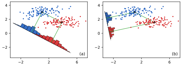
fig4_6. Download: PDF · SVG4.1.5 Relation to least squares
pp. 189–190 For two classes Fisher's direction is a least-squares solution for a particular coding of the targets. Use targets \(t_n=N/N_1\) for \(\mathcal{C}_1\) and \(t_n=-N/N_2\) for \(\mathcal{C}_2\) (roughly the reciprocal of the class prior, with a sign), and minimise
\[ E=\frac12\sum_{n=1}^N(\mathbf{w}^\T\mathbf{x}_n+w_0-t_n)^2. \tag{4.31} \]Result 4.5 (Fisher's discriminant is least squares with these targets) pp. 189–190, (4.32)–(4.38); Exercise 4.6
The minimiser satisfies
\[ w_0=-\mathbf{w}^\T\mathbf{m},\qquad \Big(\mathbf{S}_\mathrm{W}+\frac{N_1N_2}{N}\mathbf{S}_\mathrm{B}\Big)\mathbf{w}=N(\mathbf{m}_1-\mathbf{m}_2), \tag{4.34, 4.37} \]where \(\mathbf{m}\)
so the least-squares direction is Fisher's, and the rule "class \(\mathcal{C}_1\) iff \(y(\mathbf{x})\)
Proof
Bias. \(\partial E/\partial w_0\)
Weights. \(\partial E/\partial\mathbf{w}\)
Splitting \(\mathbf{S}_\mathrm{T}\). For each class, \(\sum_{n\in\mathcal{C}_k}(\mathbf{x}_n-\mathbf{m})(\mathbf{x}_n-\mathbf{m})^\T\)
Direction and sign. Let \(c=(\mathbf{m}_2-\mathbf{m}_1)^\T\mathbf{w}\), so \(\mathbf{S}_\mathrm{B}\mathbf{w}\)
Sign note. The book writes (4.38) as \(\mathbf{w}\)
4.1.6 Fisher's discriminant for multiple classes
pp. 191–192 For \(K>2\) classes and \(D>K\) take \(D'>1\) linear features \(\mathbf{y}=\mathbf{W}^\T\mathbf{x}\) (4.39), the columns of \(\mathbf{W}\) being the weight vectors (no biases). The within-class scatter generalises (4.28):
\[ \mathbf{S}_\mathrm{W}=\sum_{k=1}^K\mathbf{S}_k,\quad \mathbf{S}_k=\sum_{n\in\mathcal{C}_k}(\mathbf{x}_n-\mathbf{m}_k)(\mathbf{x}_n-\mathbf{m}_k)^\T,\quad \mathbf{m}_k=\frac1{N_k}\sum_{n\in\mathcal{C}_k}\mathbf{x}_n, \tag{4.40–4.42} \]the total scatter is \(\mathbf{S}_\mathrm{T}\)
Proof of the split (the book states it): as in the two-class proof, \(\sum_{n\in\mathcal{C}_k}(\mathbf{x}_n-\mathbf{m})(\mathbf{x}_n-\mathbf{m})^\T\)
In the projected space the same matrices are \(\mathbf{s}_\mathrm{W}\)
Erratum. The book's (4.47), (4.48), (4.50) print \(\mathbf{s}_\mathrm{W},\mathbf{s}_\mathrm{B}\) with \(s\) for the projected matrices where capital \(\mathbf{S}\) is meant, and (4.51) prints \((\mathbf{W}\mathbf{S}_\mathrm{W}\mathbf{W}^\T)^{-1}(\mathbf{W}\mathbf{S}_\mathrm{B}\mathbf{W}^\T)\); with \(\mathbf{y}=\mathbf{W}^\T\mathbf{x}\) the correct form is the one above (errata, p. 192).
Result 4.6 (the maximiser of the multiclass Fisher criterion) p. 192, "straightforward though somewhat involved"
Let \(\mathbf{S}_\mathrm{W}\succ0\) and let \(\lambda_1\ge\lambda_2\ge\dots\ge0\) be the eigenvalues of \(\mathbf{S}_\mathrm{W}^{-1}\mathbf{S}_\mathrm{B}\), with eigenvectors \(\mathbf{w}_i\) solving the generalised eigenproblem \(\mathbf{S}_\mathrm{B}\mathbf{w}_i\)
Proof
Reduction to an ordinary eigenproblem. Let \(\mathbf{S}_\mathrm{W}=\mathbf{L}\mathbf{L}^\T\) (Cholesky) and \(\mathbf{C}\)
Invariance. Put \(\widetilde{\mathbf{W}}=\mathbf{L}^\T\mathbf{W}\). Then \(\mathbf{W}^\T\mathbf{S}_\mathrm{W}\mathbf{W}\)
Upper bound (Ky Fan). Let \(\mathbf{u}_1,\dots,\mathbf{u}_D\) be orthonormal eigenvectors of \(\mathbf{C}\). Then \(\operatorname{Tr}(\mathbf{Q}^\T\mathbf{C}\mathbf{Q})\)
Rank. \(\mathbf{S}_\mathrm{B}\)
For \(K=2\) there is a single non-zero eigenvalue, with eigenvector \(\mathbf{S}_\mathrm{W}^{-1}(\mathbf{m}_2-\mathbf{m}_1)\), recovering Result 4.4. The projected features are then fed to any classifier (Fukunaga, 1990).
4.1.7 The perceptron algorithm
pp. 192–196 Rosenblatt's perceptron is a two-class model: a fixed non-linear feature vector \(\bm\phi(\mathbf{x})\) (including \(\phi_0=1\)) is passed through a step function,
\[ y(\mathbf{x})=f(\mathbf{w}^\T\bm\phi(\mathbf{x})),\qquad f(a)=\begin{cases}+1,&a\ge0\\-1,&a<0.\end{cases} \tag{4.52, 4.53} \]Targets are \(t=+1\) for \(\mathcal{C}_1\) and \(t=-1\) for \(\mathcal{C}_2\). We want \(\mathbf{w}^\T\bm\phi_nt_n>0\) for every \(n\). The number of misclassified points is a bad error function: it is piecewise constant in \(\mathbf{w}\), with zero gradient almost everywhere. The perceptron criterion is instead
\[ E_\mathrm{P}(\mathbf{w})=-\sum_{n\in\mathcal{M}}\mathbf{w}^\T\bm\phi_nt_n, \tag{4.54} \]where \(\mathcal{M}\) is the set of currently misclassified points and \(\bm\phi_n=\bm\phi(\mathbf{x}_n)\) (erratum, p. 194).
Filling the gap 4.3: what the error function looks like p. 194
Derivation
For a fixed \(n\) the term \(\max\{0,-t_n\mathbf{w}^\T\bm\phi_n\}\) is zero where \(n\) is correctly classified (\(t_n\mathbf{w}^\T\bm\phi_n\ge0\)) and the linear function \(-t_n\mathbf{w}^\T\bm\phi_n>0\) where it is not. Therefore
\[ E_\mathrm{P}(\mathbf{w})=\sum_{n=1}^N\max\{0,\,-t_n\mathbf{w}^\T\bm\phi_n\}. \]- Continuous, piecewise linear, convex: a sum of maxima of linear functions. It is non-negative and positively homogeneous, \(E_\mathrm{P}(c\mathbf{w})\)
\({}=cE_\mathrm{P}(\mathbf{w})\) for \(c>0\). - The gradient on each linear piece is \(\nabla E_\mathrm{P}\)
\({}=-\sum_{n\in\mathcal{M}}t_n\bm\phi_n\); at the kinks any member of the sub-differential is allowed. Stochastic (sub)gradient descent on one misclassified point gives \(\mathbf{w}^{(\tau+1)}\) \({}=\mathbf{w}^{(\tau)}+\eta\,t_n\bm\phi_n\) (4.55). - Degenerate minimum: \(E_\mathrm{P}=0\) exactly on the cone \(\{\mathbf{w}:t_n\mathbf{w}^\T\bm\phi_n\)
\({}\ge0\ \forall n\}\), which contains \(\mathbf{w}=\mathbf{0}\) even when the data are not separable. The algorithm does not minimise \(E_\mathrm{P}\) in the usual sense; it is the mistake-driven rule (4.55) that is analysed below.
Because \(f(a)\) is unchanged when \(\mathbf{w}\) is multiplied by a positive constant, the learning rate can be set to \(\eta=1\) without loss of generality (the sequence of \(\mathbf{w}\)'s from \(\mathbf{0}\) simply scales). ∎
Algorithm 4.1 (perceptron learning) p. 194, (4.55)
- Initialise \(\mathbf{w}=\mathbf{0}\) (any start works but the bound below is stated for this one).
- Cycle through the training points. For point \(n\), compute \(f(\mathbf{w}^\T\bm\phi_n)\).
- If \(f(\mathbf{w}^\T\bm\phi_n)\ne t_n\) (a mistake), update \(\mathbf{w}\leftarrow\mathbf{w}+t_n\bm\phi_n\): add \(\bm\phi_n\) for a point of \(\mathcal{C}_1\), subtract it for a point of \(\mathcal{C}_2\). Otherwise leave \(\mathbf{w}\) unchanged.
- Stop when a whole pass produces no mistakes.
One update reduces the error contribution of the point it was made on: using \(\eta=1\),
\[ -\mathbf{w}^{(\tau+1)\T}\bm\phi_nt_n=-\mathbf{w}^{(\tau)\T}\bm\phi_nt_n-(\bm\phi_nt_n)^\T\bm\phi_nt_n<-\mathbf{w}^{(\tau)\T}\bm\phi_nt_n, \tag{4.56} \]because \(\|\bm\phi_nt_n\|^2=\|\bm\phi_n\|^2>0\). But that does not make \(E_\mathrm{P}\) decrease: other points may become misclassified, so the criterion can go up at some steps. The following theorem is why the algorithm nevertheless works. The book only cites it.
Result 4.7 (perceptron convergence theorem; Novikoff, 1962) p. 194
Suppose the data are linearly separable with a margin: there are a unit vector \(\hat{\mathbf{w}}\) and \(\gamma>0\) with \(t_n\hat{\mathbf{w}}^\T\bm\phi_n\ge\gamma\) for all \(n\) (any finite separable set has this for some \(\gamma\)). Let \(R=\max_n\|\bm\phi_n\|\). Then Algorithm 4.1 makes at most
\[ k_{\max}=\frac{R^2}{\gamma^2} \]mistakes, for any order of presentation, and therefore halts with a separating \(\mathbf{w}\) after finitely many passes. The bound does not involve \(N\) or the dimension.
Proof
A margin exists. Separable means that some \(\mathbf{v}\) has \(t_n\mathbf{v}^\T\bm\phi_n>0\) for all \(n\) (Definition 4.1). With finitely many points \(\gamma=\min_nt_n\hat{\mathbf{w}}^\T\bm\phi_n>0\) for \(\hat{\mathbf{w}}=\mathbf{v}/\|\mathbf{v}\|\).
Let \(\mathbf{w}_k\) be the weight vector after \(k\) updates, \(\mathbf{w}_0=\mathbf{0}\), and let \(\bm\phi,t\) be the point causing the \((k+1)\)th update. At a mistake \(t\,\mathbf{w}_k^\T\bm\phi\le0\): if \(t=-1\) the mistake means \(\mathbf{w}_k^\T\bm\phi\ge0\); if \(t=+1\) it means \(\mathbf{w}_k^\T\bm\phi<0\).
Progress along \(\hat{\mathbf{w}}\). \(\hat{\mathbf{w}}^\T\mathbf{w}_{k+1}\)
Growth of the norm. \(\|\mathbf{w}_{k+1}\|^2\)
Combine. By Cauchy-Schwarz, \(k\gamma\)
Remarks. (i) For another starting vector \(\mathbf{w}_0\) the same two inequalities give \(k\gamma-\|\mathbf{w}_0\|\)
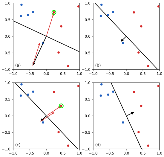
fig4_7. Download: PDF · SVGThe remaining limitations the book lists are that the perceptron has no probabilistic output, does not generalise readily to \(K>2\) classes, and, like every model of this chapter, uses fixed basis functions. Figure 4.8 of the book, a photograph of Rosenblatt's Mark 1 hardware, is not reproduced here. Widrow and Hoff's adaline (1960) had the same form but was trained by least squares on the activation.
4.2 Probabilistic generative models
pp. 196–203 Now model how the data arise: a class-conditional density \(p(\mathbf{x}\given\mathcal{C}_k)\) and a prior \(p(\mathcal{C}_k)\), and obtain the posterior by Bayes' theorem. The question is which assumptions give a linear classifier.
Result 4.8 (posterior as logistic sigmoid or softmax) pp. 197–198, (4.57)–(4.63); Exercises 4.7, 4.12
(a) For two classes, \(p(\mathcal{C}_1\given\mathbf{x})=\sigma(a)\) with \(a\)
(b) \(\sigma(-a)=1-\sigma(a)\) (4.60), \(\sigma^{-1}(y)=\ln\{y/(1-y)\}\) (the logit, 4.61), and \(\mathrm{d}\sigma/\mathrm{d}a=\sigma(1-\sigma)\) (4.88).
(c) For \(K\) classes, \(p(\mathcal{C}_k\given\mathbf{x})\)
Proof
(a) Divide numerator and denominator of Bayes' theorem by the numerator: \(p(\mathcal{C}_1\given\mathbf{x})\)
(b) \(\sigma(-a)\)
(c) Bayes' theorem gives \(p(\mathcal{C}_k\given\mathbf{x})\)
The name "softmax" is explained by the case \(a_k\gg a_j\) for all \(j\ne k\), where \(p(\mathcal{C}_k\given\mathbf{x})\approx1\): it is a smoothed arg max. Rewriting Bayes' theorem as a sigmoid is only useful if \(a(\mathbf{x})\) has a simple form; the following sections show when it is linear.
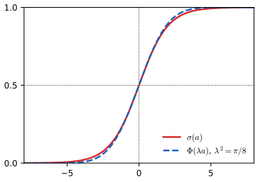
fig4_9. Download: PDF · SVG4.2.1 Continuous inputs
pp. 198–200 Let every class density be Gaussian with the same covariance \(\bm\Sigma\):
\[ p(\mathbf{x}\given\mathcal{C}_k)=\frac1{(2\pi)^{D/2}|\bm\Sigma|^{1/2}}\exp\Big\{-\tfrac12(\mathbf{x}-\bm\mu_k)^\T\bm\Sigma^{-1}(\mathbf{x}-\bm\mu_k)\Big\}. \tag{4.64} \]Result 4.9 (shared-covariance Gaussians give a linear posterior) pp. 198–199, (4.65)–(4.70); Exercise 4.8
For two classes, \(p(\mathcal{C}_1\given\mathbf{x})\)
For \(K\) classes the softmax arguments are \(a_k(\mathbf{x})=\mathbf{w}_k^\T\mathbf{x}+w_{k0}\) (4.68) with
\[ \mathbf{w}_k=\bm\Sigma^{-1}\bm\mu_k,\qquad w_{k0}=-\tfrac12\bm\mu_k^\T\bm\Sigma^{-1}\bm\mu_k+\ln p(\mathcal{C}_k). \tag{4.69, 4.70} \]Proof
By (4.58), \(a\)
and likewise for \(\bm\mu_2\). Subtracting, the quadratic terms \(-\tfrac12\mathbf{x}^\T\bm\Sigma^{-1}\mathbf{x}\) cancel, leaving \(a\)
Erratum. The book's (4.63) lacks a pair of parentheses; the correct form is \(a_k\)
Geometry. Since \(\bm\mu_1^\T\bm\Sigma^{-1}\bm\mu_1\)
The boundary \(a=0\) is perpendicular to \(\bm\Sigma^{-1}(\bm\mu_1-\bm\mu_2)\) and passes through \(\tfrac12(\bm\mu_1+\bm\mu_2)\)
Quadratic discriminant. If each class has its own \(\bm\Sigma_k\), the terms \(-\tfrac12\mathbf{x}^\T\bm\Sigma_k^{-1}\mathbf{x}\) no longer cancel and \(a_k(\mathbf{x})\)
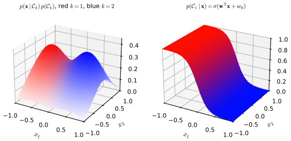
fig4_10. Download: PDF · SVG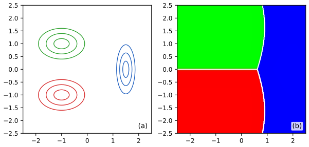
fig4_11. Download: PDF · SVG4.2.2 Maximum likelihood solution
pp. 200–202 Given labelled data \(\{\mathbf{x}_n,t_n\}\), fit the parameters by maximum likelihood. Two classes: \(t_n=1\) for \(\mathcal{C}_1\), \(t_n=0\) for \(\mathcal{C}_2\), \(p(\mathcal{C}_1)=\pi\). A point of class \(\mathcal{C}_1\) contributes \(p(\mathbf{x}_n,\mathcal{C}_1)\)
Result 4.10 (maximum likelihood for the shared-covariance Gaussian classifier) pp. 200–202, (4.72)–(4.80); Exercises 4.9, 4.10
With \(K\) classes, 1-of-\(K\) targets \(t_{nk}\) and \(N_k=\sum_nt_{nk}\):
\[ \pi_k=\frac{N_k}N,\qquad \bm\mu_k=\frac1{N_k}\sum_{n=1}^Nt_{nk}\bm\phi_n,\qquad \bm\Sigma=\sum_{k=1}^K\frac{N_k}N\mathbf{S}_k,\quad \mathbf{S}_k=\frac1{N_k}\sum_{n=1}^Nt_{nk}(\bm\phi_n-\bm\mu_k)(\bm\phi_n-\bm\mu_k)^\T. \tag{4.73, 4.75, 4.76, 4.159–4.163} \](For two classes, \(\pi=N_1/N\), \(\bm\mu_1=\frac1{N_1}\sum_nt_n\mathbf{x}_n\), \(\bm\mu_2=\frac1{N_2}\sum_n(1-t_n)\mathbf{x}_n\), \(\bm\Sigma\)
Derivation
For a general input vector (written \(\bm\phi\) as in the exercises) the log likelihood is, with each point contributing the factor of its class,
\[ \ln p=\sum_{n=1}^N\sum_{k=1}^Kt_{nk}\big\{\ln\pi_k+\ln\N(\bm\phi_n\given\bm\mu_k,\bm\Sigma)\big\}. \]Priors. Only \(\sum_{n,k}t_{nk}\ln\pi_k=\sum_kN_k\ln\pi_k\) depends on \(\bm\pi\). Maximise subject to \(\sum_k\pi_k=1\) with a multiplier: \(\partial/\partial\pi_k[\sum_jN_j\ln\pi_j+\lambda(\sum_j\pi_j-1)]\)
Means. The \(\bm\mu_k\)-dependent part is \(-\tfrac12\sum_nt_{nk}(\bm\phi_n-\bm\mu_k)^\T\bm\Sigma^{-1}(\bm\phi_n-\bm\mu_k)\)
Shared covariance. Collecting the \(\bm\Sigma\)-dependent terms, with \(\sum_k\sum_nt_{nk}=N\),
\[ -\frac N2\ln|\bm\Sigma|-\frac12\sum_{n,k}t_{nk}(\bm\phi_n-\bm\mu_k)^\T\bm\Sigma^{-1}(\bm\phi_n-\bm\mu_k)=-\frac N2\ln|\bm\Sigma|-\frac N2\operatorname{Tr}\{\bm\Sigma^{-1}\mathbf{S}\}, \tag{4.77} \]where, using \(\mathbf{a}^\T\mathbf{M}\mathbf{a}\)
Fitting Gaussians is not robust to outliers, because maximum likelihood for a Gaussian is not (Section 2.3.7).
4.2.3 Discrete features
p. 202 For binary features \(x_i\in\{0,1\}\), \(i=1,\dots,D\), a general class-conditional distribution needs \(2^D-1\) numbers per class. The naive Bayes assumption (features independent given the class, Section 8.2.2) uses \(D\):
\[ p(\mathbf{x}\given\mathcal{C}_k)=\prod_{i=1}^D\mu_{ki}^{x_i}(1-\mu_{ki})^{1-x_i}. \tag{4.81} \]Substituting into (4.63),
\[ a_k(\mathbf{x})=\sum_{i=1}^D\{x_i\ln\mu_{ki}+(1-x_i)\ln(1-\mu_{ki})\}+\ln p(\mathcal{C}_k), \tag{4.82} \]which is linear in \(\mathbf{x}\): slope \(\ln\frac{\mu_{ki}}{1-\mu_{ki}}\) on \(x_i\), intercept \(\sum_i\ln(1-\mu_{ki})+\ln p(\mathcal{C}_k)\). For two classes, \(a\)
Filling the gap 4.4: features with \(L\) states (naive Bayes) p. 202; Exercise 4.11
Let \(\bm\phi\) have \(M\) components, each coded 1-of-\(L\): \(\phi_{il}\in\{0,1\}\), \(\sum_l\phi_{il}=1\), and given \(\mathcal{C}_k\) the components are independent with \(P(\phi_{il}=1\given\mathcal{C}_k)=\mu_{kil}\), \(\sum_l\mu_{kil}=1\).
Derivation
Component \(i\) has the categorical probability \(\prod_{l=1}^L\mu_{kil}^{\phi_{il}}\) (exactly one exponent is 1). Independence gives \(p(\bm\phi\given\mathcal{C}_k)\)
linear in the components \(\phi_{il}\) of \(\bm\phi\). (With \(L=2\) this is (4.82).) The ML estimate maximises \(\sum_{n\in\mathcal{C}_k}\sum_l\phi_{nil}\ln\mu_{kil}\) subject to \(\sum_l\mu_{kil}=1\); a Lagrange multiplier gives \(\mu_{kil}\)
4.2.4 Exponential family
pp. 202–203 Both cases are instances of one result. Take class-conditional densities in the exponential family (2.194) with \(\mathbf{u}(\mathbf{x})=\mathbf{x}\) and a scaling parameter \(s\) common to all classes (2.236):
\[ p(\mathbf{x}\given\bm\lambda_k,s)=\frac1sh\Big(\frac1s\mathbf{x}\Big)g(\bm\lambda_k)\exp\Big\{\frac1s\bm\lambda_k^\T\mathbf{x}\Big\}. \tag{4.83, 4.84} \]Result 4.11 (exponential-family class densities give a generalised linear posterior) p. 203, (4.85), (4.86)
For two classes \(p(\mathcal{C}_1\given\mathbf{x})\)
both linear in \(\mathbf{x}\). The factor \(\frac1sh(\mathbf{x}/s)\) is common to all classes and cancels.
Proof
By (4.58) and (4.63) take logs: \(a_k\)
(The errata mention a missing factor \(1/s\) in the first term of (4.85) and (4.86); the printing used here already has it.) Checks. A Gaussian with shared \(\bm\Sigma\) has the form (4.84) with \(s=1\), \(\bm\lambda_k=\bm\Sigma^{-1}\bm\mu_k\), \(g(\bm\lambda)\)
4.3 Probabilistic discriminative models
pp. 203–213 Section 4.2 fitted class densities and then inverted them. The alternative is to write the generalised linear model for \(p(\mathcal{C}_k\given\bm\phi)\) down directly and maximise the conditional likelihood. This is discriminative training. It models less (no density of \(\mathbf{x}\)), typically needs fewer parameters, and can predict better when the class-density assumptions are wrong. The price is that the data cannot be generated from the model. For \(\bm\phi\in\R^M\), logistic regression has \(M\) parameters; fitting Gaussians with a shared covariance instead needs \(2M\) (means) \(+\,M(M+1)/2\) (covariance) \(+\,1\) (prior) \(=M(M+5)/2+1\), quadratic in \(M\).
4.3.1 Fixed basis functions
pp. 204–205 Everything so far works equally on \(\bm\phi(\mathbf{x})\) in place of \(\mathbf{x}\): decision boundaries are linear in feature space, non-linear in input space, and classes inseparable in \(\mathbf{x}\) can become separable in \(\bm\phi\) (Figure 4.12). One basis function is conventionally \(\phi_0=1\), carrying the bias. A fixed \(\bm\phi\) cannot remove class overlap, because \(p(\mathcal{C}_k\given\mathbf{x})\) already lies strictly between 0 and 1 there and the posterior is a function of \(\mathbf{x}\) only; it can even create overlap (a many-to-one map identifies inputs of different classes) or make the posterior easier to model. The limitation that the basis is fixed motivates the adaptive models of later chapters (Section 3.6).
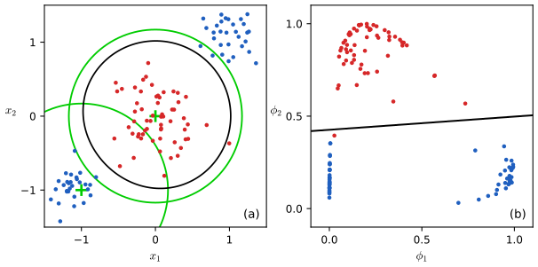
fig4_12. Download: PDF · SVG4.3.2 Logistic regression
pp. 205–206 For two classes the model is
\[ p(\mathcal{C}_1\given\bm\phi)=y(\bm\phi)=\sigma(\mathbf{w}^\T\bm\phi),\qquad p(\mathcal{C}_2\given\bm\phi)=1-y(\bm\phi). \tag{4.87} \](Despite the name, this is a classification model.) For targets \(t_n\in\{0,1\}\), \(y_n=\sigma(a_n)\), \(a_n=\mathbf{w}^\T\bm\phi_n\), the likelihood of independent Bernoulli observations is
\[ p(\mathbf{t}\given\mathbf{w})=\prod_{n=1}^Ny_n^{t_n}\{1-y_n\}^{1-t_n}, \tag{4.89} \]and the negative log likelihood is the cross-entropy error
\[ E(\mathbf{w})=-\ln p(\mathbf{t}\given\mathbf{w})=-\sum_{n=1}^N\{t_n\ln y_n+(1-t_n)\ln(1-y_n)\}. \tag{4.90} \]Result 4.12 (gradient of the cross-entropy) p. 206, (4.88), (4.91); Exercises 4.12, 4.13
\[ \nabla E(\mathbf{w})=\sum_{n=1}^N(y_n-t_n)\bm\phi_n. \tag{4.91} \]Proof
With \(\d y_n/\d a_n=y_n(1-y_n)\) (4.88; Result 4.8(b)) and \(\nabla a_n=\bm\phi_n\), the chain rule gives
\[ \nabla E=-\sum_n\Big\{\frac{t_n}{y_n}-\frac{1-t_n}{1-y_n}\Big\}y_n(1-y_n)\bm\phi_n=-\sum_n\{t_n(1-y_n)-(1-t_n)y_n\}\bm\phi_n=\sum_n(y_n-t_n)\bm\phi_n. \]The factor \(y_n(1-y_n)\) of the sigmoid derivative cancels the denominator. ∎
The factor \(\sigma'\) cancels and the contribution of point \(n\) is its "error" \(y_n-t_n\) times \(\bm\phi_n\), the same form as the gradient of the sum-of-squares error for linear regression (3.13). A sequential algorithm updates with one term at a time. A numerically safe form of the error is \(E=\sum_n\{\ln(1+e^{a_n})-t_na_n\}\), obtained by substituting \(y_n=\sigma(a_n)\) in (4.90) (use \(\operatorname{logaddexp}\)).
Result 4.13 (separable data: the maximum-likelihood weights diverge) p. 206; Exercise 4.14
If the data are linearly separable, \(E(\mathbf{w})>0\) for every finite \(\mathbf{w}\) yet \(\inf_{\mathbf{w}}E=0\), so no maximum-likelihood solution exists. Any separating direction \(\hat{\mathbf{w}}\) (i.e. \(\hat{\mathbf{w}}^\T\bm\phi_n>0\) for \(t_n=1\) and \(<0\) for \(t_n=0\)) gives \(E(c\hat{\mathbf{w}})\to0\) as \(c\to\infty\): the likelihood is maximised by \(\|\mathbf{w}\|\to\infty\) along a separating hyperplane. The singularity is removed by a prior (MAP) or an added penalty \(\frac\alpha2\mathbf{w}^\T\mathbf{w}\).
Proof
Each \(y_n\in(0,1)\) for finite \(a_n\), so every term of (4.90) is strictly positive and \(E>0\). For a separating \(\hat{\mathbf{w}}\), \(\hat a_n=\hat{\mathbf{w}}^\T\bm\phi_n\) has the sign \(+\) when \(t_n=1\) and \(-\) when \(t_n=0\). As \(c\to\infty\), \(\sigma(c\hat a_n)\to1\) if \(t_n=1\) and \(\to0\) if \(t_n=0\); in both cases the probability of the observed class tends to 1 and its \(-\ln\) to 0. Hence \(E(c\hat{\mathbf{w}})\to0\) while never reaching it. The posterior of every training point tends to 0 or 1, and the sigmoid in feature space tends to a Heaviside step. There is a continuum of separating directions, all with the same limit, and maximum likelihood cannot choose between them: the result depends on the optimiser and initialisation (compare Figure 10.13). Adding \(\frac\alpha2\|\mathbf{w}\|^2\) makes the objective coercive (it tends to infinity with \(\|\mathbf{w}\|\)), so a minimiser exists. ∎
The problem does not go away with more data: it occurs whenever the training set is separable, even if \(N\gg M\).
4.3.3 Iterative reweighted least squares
pp. 207–208 The logistic-regression error has no closed-form minimiser, but it is convex and close to quadratic, so Newton-Raphson works well. For minimising \(E(\mathbf{w})\) it updates
\[ \mathbf{w}^{(\mathrm{new})}=\mathbf{w}^{(\mathrm{old})}-\mathbf{H}^{-1}\nabla E(\mathbf{w}), \tag{4.92} \]with \(\mathbf{H}=\nabla\nabla E\) the Hessian.
Filling the gap 4.5: why (4.92), and the linear-regression check pp. 207–208, (4.93)–(4.95)
Derivation
Expand \(E\) around the current point to second order, \(E(\mathbf{w})\)
Linear regression. For \(E=\tfrac12\sum_n(\mathbf{w}^\T\bm\phi_n-t_n)^2\), \(\nabla E\)
Result 4.14 (Hessian of the cross-entropy; convexity) pp. 207–208, (4.96)–(4.98); Exercise 4.15
With \(\mathbf{y}=(y_1,\dots,y_N)^\T\) and \(\mathbf{R}=\diag(y_n(1-y_n))\) (4.98),
\[ \nabla E=\bm\Phi^\T(\mathbf{y}-\mathbf{t}),\qquad \mathbf{H}=\nabla\nabla E=\sum_{n=1}^Ny_n(1-y_n)\bm\phi_n\bm\phi_n^\T=\bm\Phi^\T\mathbf{R}\bm\Phi. \tag{4.96, 4.97} \]\(\mathbf{H}\) is positive semi-definite for every \(\mathbf{w}\), and positive definite if \(\bm\Phi\) has rank \(M\). Hence \(E\) is convex, and strictly convex when \(\operatorname{rank}\bm\Phi=M\), so it has at most one minimiser; it has exactly one unless the data are separable (Result 4.13).
Proof
Differentiate (4.91) once more: \(\nabla\nabla E\)
since \(0<y_n<1\) (a sigmoid never reaches 0 or 1). The sum is zero iff \(\mathbf{u}^\T\bm\phi_n=0\) for all \(n\), i.e. \(\bm\Phi\mathbf{u}=\mathbf{0}\); this forces \(\mathbf{u}=\mathbf{0}\) exactly when \(\bm\Phi\) has full column rank. A twice-differentiable function with everywhere positive semi-definite Hessian is convex, and with positive definite Hessian strictly convex, whose stationary point (if any) is the unique minimum. ∎
Erratum. The last line of Exercise 4.15 says "concave"; it is "convex" (errata). The book's text (p. 208) states the Hessian is positive definite for arbitrary \(\mathbf{u}\); that requires \(\operatorname{rank}\bm\Phi=M\), as shown.
Filling the gap 4.6: the IRLS update and its interpretation pp. 208–209, (4.99)–(4.103)
Derivation
Newton step. Insert (4.96), (4.97) in (4.92):
\[ \mathbf{w}^{(\mathrm{new})}=\mathbf{w}^{(\mathrm{old})}-(\bm\Phi^\T\mathbf{R}\bm\Phi)^{-1}\bm\Phi^\T(\mathbf{y}-\mathbf{t})=(\bm\Phi^\T\mathbf{R}\bm\Phi)^{-1}\bm\Phi^\T\mathbf{R}\mathbf{z}, \tag{4.99} \]where \(\mathbf{z}\)
This is the normal equation of a weighted least-squares problem, \(\min_{\mathbf{w}}\sum_nR_{nn}(z_n-\mathbf{w}^\T\bm\phi_n)^2\), with weights \(R_{nn}\) that depend on \(\mathbf{w}\); hence the name iterative reweighted least squares (Rubin, 1983): solve, recompute \(\mathbf{y}\), \(\mathbf{R}\), \(\mathbf{z}\), repeat.
The weights are variances. For \(t\in\{0,1\}\) with \(P(t=1)=y\): \(\mathbb{E}[t]=y\) (4.101) and, since \(t^2=t\), \(\operatorname{var}[t]\)
The effective target. Linearise the activation as a function of \(y\) around the current point. From \(y=\sigma(a)\), \(\d a/\d y=1/\{y(1-y)\}\). Then
\[ a_n(\mathbf{w})\simeq a_n(\mathbf{w}^{(\mathrm{old})})+\frac{\d a_n}{\d y_n}(t_n-y_n)=\bm\phi_n^\T\mathbf{w}^{(\mathrm{old})}-\frac{y_n-t_n}{y_n(1-y_n)}=z_n, \tag{4.103} \]i.e. \(z_n\) is the value of the activation \(a\) at which the linearised sigmoid would hit the target \(t_n\): the "working response". IRLS fits a linear model to these working responses by weighted least squares. ∎
Algorithm 4.2 (IRLS for two-class logistic regression) pp. 207–209
- Initialise \(\mathbf{w}\) (for example \(\mathbf{0}\), which gives \(y_n=\tfrac12\), \(\mathbf{R}=\tfrac14\mathbf{I}\)).
- Compute \(a_n=\mathbf{w}^\T\bm\phi_n\), \(y_n=\sigma(a_n)\), \(R_{nn}=y_n(1-y_n)\), and \(\mathbf{z}\)
\({}=\bm\Phi\mathbf{w}\) \({}-\mathbf{R}^{-1}(\mathbf{y}-\mathbf{t})\). - Solve \((\bm\Phi^\T\mathbf{R}\bm\Phi)\mathbf{w}^{(\mathrm{new})}\)
\({}=\bm\Phi^\T\mathbf{R}\mathbf{z}\) (cost \(O(NM^2+M^3)\) per step). - Repeat until \(\|\nabla E\|\) is small. With a penalty \(\frac\alpha2\|\mathbf{w}\|^2\) use \(\bm\Phi^\T\mathbf{R}\bm\Phi+\alpha\mathbf{I}\) and add \(\alpha\mathbf{w}\) to the gradient; this also keeps the system solvable on separable data.
Convergence. Near the minimum the convergence is quadratic (standard Newton theory: the error is squared at each step). Far from it, Newton's step can overshoot because \(E\) is not quadratic, so robust implementations add a line search or damping. Because the logistic model uses the canonical link (Section 4.3.6), the Hessian does not depend on the targets, so IRLS is the same as Fisher scoring. On separable data (Result 4.13) \(R_{nn}\to0\) and \(\bm\Phi^\T\mathbf{R}\bm\Phi\) becomes nearly singular: IRLS does not converge but drives \(\|\mathbf{w}\|\) to infinity, with a surprisingly regular pattern. In the one-point example \(\phi=1\), \(t=1\), \(E(w)=\ln(1+e^{-w})\), the Newton step is \(-E'/E''=1/\{\sigma(w)\}\), which tends to 1 as \(w\) grows: the weight increases by about one per iteration (computed: \(w\)
4.3.4 Multiclass logistic regression
pp. 209–210 For \(K\) classes use the softmax of linear activations,
\[ p(\mathcal{C}_k\given\bm\phi)=y_k(\bm\phi)=\frac{\exp(a_k)}{\sum_j\exp(a_j)},\qquad a_k=\mathbf{w}_k^\T\bm\phi. \tag{4.104, 4.105} \]With 1-of-\(K\) targets \(\mathbf{t}_n\) (matrix \(\mathbf{T}\), entries \(t_{nk}\)) and \(y_{nk}=y_k(\bm\phi_n)\), the likelihood and cross-entropy error are
\[ p(\mathbf{T}\given\mathbf{w}_1,\dots,\mathbf{w}_K)=\prod_{n=1}^N\prod_{k=1}^Ky_{nk}^{t_{nk}},\qquad E(\mathbf{w}_1,\dots,\mathbf{w}_K)=-\sum_{n=1}^N\sum_{k=1}^Kt_{nk}\ln y_{nk}. \tag{4.107, 4.108} \]Result 4.15 (derivatives of softmax and the multiclass cross-entropy) pp. 209–210, (4.106), (4.109), (4.110); Exercises 4.17, 4.18, 4.20
(a) \(\dfrac{\partial y_k}{\partial a_j}\)
(d) The full \(MK\times MK\) Hessian is positive semi-definite, so \(E\) is convex. It is not positive definite: it always has the null space \(\{(\mathbf{u},\dots,\mathbf{u})\}\) of dimension at least \(M\).
Proof
(a) \(y_k=e^{a_k}/S\), \(S=\sum_je^{a_j}\), \(\partial S/\partial a_j=e^{a_j}\). Quotient rule: \(\dfrac{\partial y_k}{\partial a_j}\)
(b) \(\partial E/\partial a_{nj}\)
(c) Differentiate (4.109) with respect to \(\mathbf{w}_k\): by (a), \(\nabla_{\mathbf{w}_k}y_{nj}\)
(d) Let \(\mathbf{u}=(\mathbf{u}_1,\dots,\mathbf{u}_K)\) and \(b_{nk}=\mathbf{u}_k^\T\bm\phi_n\). Then
\[ \mathbf{u}^\T\mathbf{H}\mathbf{u}=\sum_n\sum_{j,k}b_{nj}\,y_{nj}(I_{jk}-y_{nk})\,b_{nk}=\sum_n\Big\{\sum_ky_{nk}b_{nk}^2-\Big(\sum_ky_{nk}b_{nk}\Big)^2\Big\}. \]For each \(n\), \((y_{n1},\dots,y_{nK})\) is a probability vector, so the bracket is the variance of \(b_{n\cdot}\) under it, \(\mathbb{E}[b^2]-\mathbb{E}[b]^2\ge0\) (Jensen's inequality for the convex square, toolkit). So \(\mathbf{H}\succeq0\). The bracket is zero if \(b_{nk}\) is the same for all \(k\), e.g. \(\mathbf{u}_1=\dots=\mathbf{u}_K\): adding the same vector to every \(\mathbf{w}_k\) multiplies every \(e^{a_k}\) by the same factor and does not change the model. ∎
Erratum. The leading minus sign in the book's (4.110) is removed in the errata; the form above has it removed. The book's sentence "positive definite" (p. 210) should read "positive semi-definite", as in Exercise 4.20; strict convexity is restored by fixing one weight vector at zero or by a penalty \(\frac\alpha2\sum_k\|\mathbf{w}_k\|^2\).
The gradient has the same "error times feature" form as linear regression and two-class logistic regression, an instance of the canonical-link result (Result 4.17). The Newton-Raphson (IRLS) update uses the block Hessian (4.110) and gradient (4.109); a practical implementation fixes \(\mathbf{w}_K=\mathbf{0}\) (or adds a ridge) so that the \(M(K-1)\times M(K-1)\) system is non-singular (Bishop and Nabney, 2008). A Figure 4.5-style comparison shows the effect: logistic regression separates the three classes on which least squares masks one.
4.3.5 Probit regression
pp. 210–212 Not every class-conditional model gives a logistic posterior (Gaussian mixtures do not), so other link functions are worth considering within the generalised linear model \(p(t=1\given a)=f(a)\), \(a=\mathbf{w}^\T\bm\phi\) (4.111). One motivation is a noisy threshold model: set \(t_n=1\) if \(a_n\ge\theta\) and \(t_n=0\) otherwise (4.112), with \(\theta\) drawn at random from a density \(p(\theta)\). Then
\[ p(t=1\given a)=P(\theta\le a)=f(a)=\int_{-\infty}^ap(\theta)\,\d\theta, \tag{4.113} \]the cumulative distribution function of \(\theta\) (Figure 4.13: the density is the slope of the cdf, the cdf is the area under the density). For a standard normal \(\theta\),
\[ \Phi(a)=\int_{-\infty}^a\N(\theta\given0,1)\,\d\theta, \tag{4.114} \]the inverse probit function (the probit is its inverse; errata). A \(\theta\) with another mean and variance is absorbed in the bias and in the scale of \(\mathbf{w}\), so nothing is lost. Many libraries provide instead the error function, with the corrected definition
\[ \operatorname{erf}(a)=\frac2{\sqrt\pi}\int_0^a\exp(-\theta^2)\,\d\theta,\qquad \Phi(a)=\frac12\Big\{1+\operatorname{erf}\Big(\frac a{\sqrt2}\Big)\Big\}. \tag{4.115, 4.116} \]Erratum. The book's (4.115) has a factor \(\tfrac12\) in the exponent (\(\exp(-\theta^2/2)\)); the correct integrand is \(\exp(-\theta^2)\), as above. (4.116) is the corrected relation, with \(\Phi\) not bold.
Filling the gap 4.7: \(\Phi\) and erf; the probit gradient and Hessian pp. 211–212; Exercises 4.19, 4.21
Derivation
(4.116). By symmetry of the standard normal about 0, \(\Phi(a)\)
Gradient. With \(y_n=\Phi(a_n)\), \(a_n=\mathbf{w}^\T\bm\phi_n\), and \(\Phi'(a)=\N(a\given0,1)=:\varphi(a)\), the error is \(E=-\sum_n\{t_n\ln y_n+(1-t_n)\ln(1-y_n)\}\), and as in the logistic case
\[ \nabla E=\sum_n\frac{y_n-t_n}{y_n(1-y_n)}\,\varphi(a_n)\,\bm\phi_n. \](For the logistic link \(\varphi\) is replaced by \(y(1-y)\), which cancels the denominator; for the probit it does not, so the simple "error times feature" form is lost: the probit link is not canonical.) Hessian. Write \(\nabla E=\sum_n g(a_n)\bm\phi_n\) with \(g(a)=(y-t)\nu(a)\), \(\nu=\varphi/\{y(1-y)\}\). Then \(\mathbf{H}=\sum_ng'(a_n)\bm\phi_n\bm\phi_n^\T\), where using \(\varphi'(a)=-a\varphi(a)\), \(y'=\varphi\) and \(\nu'\)
IRLS for the probit model is then (4.92) with this gradient and Hessian (I checked both against finite differences on random data). ∎
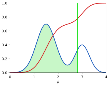
fig4_13. Download: PDF · SVGLogit versus probit. The two fits are usually similar. Since \(\sigma(a)\approx\Phi(\lambda a)\) with \(\lambda^2=\pi/8\) (Figure 4.9), logistic weights are expected to be about \(1/\lambda\approx1.6\) times the probit weights (in our demo fits the ratio \(|\mathbf{w}_\mathrm{probit}|/|\mathbf{w}_\mathrm{logistic}|\) is about 0.59, against \(1/\lambda=1.596\) for the exact reciprocal 0.63). They differ in the tails: \(1-\sigma(a)\sim e^{-a}\) but \(1-\Phi(a)\sim e^{-a^2/2}/a\), so a point far on the wrong side of the boundary (an outlier or a mislabel) costs only linearly in the logistic error but quadratically in the probit error, which makes probit regression more sensitive to such points. Both assume correct labels. Mislabelling with flip probability \(\epsilon\) is modelled by
\[ p(t\given\mathbf{x})=(1-\epsilon)\sigma(\mathbf{x})+\epsilon\{1-\sigma(\mathbf{x})\}=\epsilon+(1-2\epsilon)\sigma(\mathbf{x}), \tag{4.117} \]with \(\epsilon\) fixed or inferred (Opper and Winther, 2000). The label is \(t=1\) either if it is truly 1 and not flipped, or truly 0 and flipped; the second form follows by expanding. The posterior is then squeezed into \([\epsilon,1-\epsilon]\), so a point far from the boundary has a bounded cost \(-\ln\epsilon\).
4.3.6 Canonical link functions
pp. 212–213 The simple gradient "(prediction minus target) times feature" appeared for linear regression (3.12), the sigmoid with cross-entropy (4.90) and the softmax with its cross-entropy (4.108). It is a general property of the exponential family with the right link. Let the target have the conditional density (cf. (4.84), here applied to \(t\), not to the input)
\[ p(t\given\eta,s)=\frac1sh\Big(\frac ts\Big)g(\eta)\exp\Big\{\frac{\eta t}s\Big\}. \tag{4.118} \]Result 4.16 (mean and variance of the exponential-family target) p. 212, (4.119)
\[ y\equiv\mathbb{E}[t\given\eta]=-s\frac{\d}{\d\eta}\ln g(\eta),\qquad \operatorname{var}[t\given\eta]=s\frac{\d y}{\d\eta}. \tag{4.119} \]Proof
Normalisation: \(g(\eta)\int\frac1sh(t/s)\exp(\eta t/s)\,\d t=1\). Differentiate with respect to \(\eta\) (the argument of the toolkit's exponential-family moments): \(\frac{g'}g+\frac{\mathbb{E}[t]}s=0\), so \(\mathbb{E}[t]=-s\,\d\ln g/\d\eta\). For the variance, note \(\partial p/\partial\eta=p\,(g'/g+t/s)=p\,(t-y)/s\). Hence \(\d y/\d\eta\)
So \(y\) and \(\eta\) are linked, \(\eta=\psi(y)\). A generalised linear model (Nelder and Wedderburn, 1972) has \(y=f(\mathbf{w}^\T\bm\phi)\) (4.120): \(f\) is the activation function, \(f^{-1}\) the link function.
Result 4.17 (the canonical link gives the error-times-feature gradient) pp. 213, (4.121)–(4.124)
For data \(\{\bm\phi_n,t_n\}\) with a common scale \(s\), the gradient of the log likelihood is
\[ \nabla_{\mathbf{w}}\ln p(\mathbf{t}\given\bm\eta,s)=\sum_{n=1}^N\frac1s\{t_n-y_n\}\,\psi'(y_n)f'(a_n)\bm\phi_n, \tag{4.122} \]with \(a_n=\mathbf{w}^\T\bm\phi_n\). If the link is the canonical one, \(f^{-1}=\psi\) (4.123), then \(\psi'(y)f'(a)=1\) and the gradient of the error \(E=-\ln p\) is
\[ \nabla E(\mathbf{w})=\frac1s\sum_{n=1}^N\{y_n-t_n\}\bm\phi_n. \tag{4.124} \]Proof
The log likelihood is \(\sum_n\{\ln g(\eta_n)+\eta_nt_n/s\}\)
so the brace is \((t_n-y_n)/s\), \(\d\eta_n/\d y_n=\psi'(y_n)\), \(\d y_n/\d a_n=f'(a_n)\): this is (4.122). If \(f^{-1}=\psi\) then \(f(\psi(y))=y\), and differentiating, \(f'(\psi(y))\psi'(y)=1\); also \(a=f^{-1}(y)=\psi(y)\), so \(f'(a)\psi'(y)=1\). The factor drops out and the sign change gives (4.124). ∎
Examples. (i) Gaussian target with precision \(\beta\): \(s=\beta^{-1}\), \(\eta=\mu\), \(g(\eta)=e^{-\beta\eta^2/2}\), \(y=-s\,\d\ln g/\d\eta=\eta\), so the canonical link is the identity (linear regression). (ii) Bernoulli: \(s=1\), \(\eta=\ln\frac y{1-y}\), \(g=1-y=\sigma(-\eta)\), \(y=\sigma(\eta)\): the logit link, hence logistic regression. (iii) Categorical: the softmax. (iv) Poisson: \(p(t)=\lambda^te^{-\lambda}/t!\) has \(\eta=\ln\lambda\), \(g(\eta)=\exp(-e^\eta)\), \(y=\lambda\), so the canonical link is the log, \(\lambda=\exp(\mathbf{w}^\T\bm\phi)\), and again \(\nabla E=\sum_n(y_n-t_n)\bm\phi_n\). The probit link is not canonical for the Bernoulli distribution, as the gradient above shows.
For a canonical link the Hessian is \(\frac1s\sum_nf'(a_n)\bm\phi_n\bm\phi_n^\T\) (differentiate (4.124) once, with \(\d y_n/\d a_n=f'(a_n)\)), which does not contain the targets: Newton-Raphson then equals Fisher scoring, and for the Bernoulli case it is (4.97).
4.4 The Laplace approximation
pp. 213–217 The posterior of logistic regression is not Gaussian, so the Bayesian treatment of Section 3.3 cannot be copied. The Laplace approximation fits a Gaussian to a density by matching its mode and its curvature there. Let \(p(z)=f(z)/Z\) be a density of one continuous variable with unknown normaliser \(Z=\int f(z)\,\d z\) (4.125).
Algorithm 4.3 (Laplace approximation, one variable) pp. 213–214, (4.126)–(4.130)
- Find a mode \(z_0\) of \(p\): a point with \(\mathrm{d}f/\mathrm{d}z=0\) (4.126), by numerical optimisation of \(\ln f\).
- Compute \(A=-\dfrac{\d^2}{\d z^2}\ln f(z)\Big|_{z=z_0}\) (4.128); it must be positive for \(z_0\) to be a local maximum.
- Return \(q(z)=\N(z\given z_0,A^{-1})\) (4.130).
Filling the gap 4.8: the one-dimensional derivation pp. 214–215, (4.127)–(4.130)
Derivation
A Gaussian has a quadratic logarithm, so expand \(\ln f\) to second order about the mode \(z_0\). The first-order term is \((\ln f)'(z_0)(z-z_0)\)
Exponentiating, \(f(z)\simeq f(z_0)\exp\{-\tfrac A2(z-z_0)^2\}\) (4.129). This is proportional to a Gaussian with mean \(z_0\) and variance \(1/A\) when \(A>0\); the normaliser follows from \(\int\exp\{-\tfrac A2(z-z_0)^2\}\d z\)
Neither the mode nor \(A\) needs the unknown \(Z\), because \(\ln Z\) is a constant that disappears under \(\d/\d z\). ∎
Example (Figure 4.14). For \(f(z)=e^{-z^2/2}\sigma(20z+4)\), \(\ln f=-z^2/2+\ln\sigma(20z+4)\); the mode solves \(z=20\{1-\sigma(20z+4)\}\), and \(A=1+400\,\sigma(20z_0+4)\{1-\sigma(20z_0+4)\}\). Numerically (my computation) \(z_0=0.0775\) and \(A=2.54\); the exact normaliser is \(Z=\int f\,\d z=1.451\) while the Laplace estimate (4.135) is \(f(z_0)\sqrt{2\pi/A}=1.561\), about 8% high. The true density is skewed (heavier on the side where the sigmoid is flat), so a symmetric Gaussian cannot match it; the right panel (negative logs) shows the quadratic against the true curve.
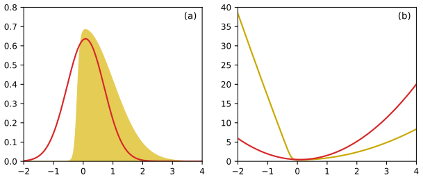
fig4_14. Download: PDF · SVGSeveral variables
For \(\mathbf{z}\in\R^M\) and \(p(\mathbf{z})=f(\mathbf{z})/Z\), at a stationary point \(\mathbf{z}_0\) (\(\nabla f=\mathbf{0}\)) the second-order expansion is
\[ \ln f(\mathbf{z})\simeq\ln f(\mathbf{z}_0)-\tfrac12(\mathbf{z}-\mathbf{z}_0)^\T\mathbf{A}(\mathbf{z}-\mathbf{z}_0),\qquad \mathbf{A}=-\nabla\nabla\ln f(\mathbf{z})\big|_{\mathbf{z}=\mathbf{z}_0}, \tag{4.131, 4.132} \]the linear term vanishing because \(\nabla\ln f=\nabla f/f=\mathbf{0}\), and the Hessian being symmetric. Exponentiating gives (4.133). Comparing with the Gaussian density (2.43), the normalised approximation is
\[ q(\mathbf{z})=\frac{|\mathbf{A}|^{1/2}}{(2\pi)^{M/2}}\exp\Big\{-\tfrac12(\mathbf{z}-\mathbf{z}_0)^\T\mathbf{A}(\mathbf{z}-\mathbf{z}_0)\Big\}=\N(\mathbf{z}\given\mathbf{z}_0,\mathbf{A}^{-1}). \tag{4.134} \]It is a proper density iff \(\mathbf{A}\succ0\), i.e. the stationary point is a local maximum, not a minimum or saddle.
Properties and limits
- Easy to apply: it needs a mode (numerical optimisation) and one Hessian, not \(Z\). Multimodal densities give a different approximation per mode.
- Large \(N\): as the data accumulate the posterior concentrates and becomes nearly Gaussian (central limit behaviour), so the approximation improves.
- Real variables only, and not invariant to re-parametrisation. Example: a Gamma-shaped \(p(\tau)\propto\tau^{a-1}e^{-b\tau}\) has mode \((a-1)/b\) in \(\tau\), but in \(u=\ln\tau\) the density is \(\propto e^{au-be^u}\) with mode \(\ln(a/b)\) and curvature \(a\); a Laplace approximation in \(u\) is a log-normal in \(\tau\) with median \(a/b\), different from the Gaussian in \(\tau\). One chooses a parametrisation in which the posterior is closer to Gaussian (for a positive scale, its log).
- Local: it uses only the neighbourhood of one point and can miss global properties (the skew in Figure 4.14, mass in other modes). Chapter 10 gives global alternatives.
4.4.1 Model comparison and BIC
pp. 216–217 The same expansion approximates the normaliser:
\[ Z=\int f(\mathbf{z})\,\d\mathbf{z}\simeq f(\mathbf{z}_0)\int\exp\Big\{-\tfrac12(\mathbf{z}-\mathbf{z}_0)^\T\mathbf{A}(\mathbf{z}-\mathbf{z}_0)\Big\}\d\mathbf{z}=f(\mathbf{z}_0)\frac{(2\pi)^{M/2}}{|\mathbf{A}|^{1/2}}, \tag{4.135} \]because the integrand is an unnormalised Gaussian whose integral is the reciprocal of the constant in (4.134). Apply this to the model evidence (Section 3.4) of a model with parameters \(\bm\theta\in\R^M\),
\[ p(\mathcal{D})=\int p(\mathcal{D}\given\bm\theta)p(\bm\theta)\,\d\bm\theta, \tag{4.136} \]identifying \(f(\bm\theta)\)
Result 4.18 (Laplace approximation to the log evidence; Occam factor) p. 216, (4.137), (4.138); Exercise 4.22
\[ \ln p(\mathcal{D})\simeq\underbrace{\ln p(\mathcal{D}\given\bm\theta_\mathrm{MAP})}_{\text{best fit}}+\underbrace{\ln p(\bm\theta_\mathrm{MAP})+\frac M2\ln(2\pi)-\frac12\ln|\mathbf{A}|}_{\text{Occam factor}}, \tag{4.137} \]where \(\bm\theta_\mathrm{MAP}\) is the posterior mode and \(\mathbf{A}\)
Proof
Take the logarithm of (4.135) with \(f=p(\mathcal{D}\given\bm\theta)p(\bm\theta)\): \(\ln p(\mathcal{D})\)
Why "Occam factor". In one dimension \(\exp(\text{Occam})\)
Result 4.19 (BIC as a large-\(N\) limit of the Laplace evidence) p. 217, (4.139); Exercise 4.23
If the prior is broad and the Hessian has full rank, and the data are i.i.d., then
\[ \ln p(\mathcal{D})\simeq\ln p(\mathcal{D}\given\bm\theta_\mathrm{MAP})-\frac12M\ln N. \tag{4.139} \]Proof
Take a Gaussian prior \(p(\bm\theta)\)
For a broad prior \(\mathbf{V}_0^{-1}\) is small: the quadratic term and \(\mathbf{V}_0^{-1}\) inside the determinant are negligible, and \(\ln|\mathbf{V}_0|\) is a constant not growing with \(N\): \(\ln p(\mathcal{D})\)
(4.139) is the Bayesian information criterion (Schwarz, 1978). Compared with the Akaike criterion (1.73), \(\ln p(\mathcal{D}\given\mathbf{w}_\mathrm{ML})-M\), its penalty \(\frac12M\ln N\) is heavier once \(\ln N>2\), i.e. \(N>e^2\approx7.4\). Both are cheap but crude: the full-rank assumption fails when some parameters are poorly determined by the data (the "well-determined parameters" of Section 3.5.3), and then (4.137) with the actual \(\mathbf{A}\) is more accurate, as Section 5.7 illustrates for neural networks. Note that (4.139) replaces the posterior mode by the log likelihood at \(\bm\theta_\mathrm{MAP}\); at large \(N\) the maximum-likelihood value is equivalent.
4.5 Bayesian logistic regression
pp. 217–220 Exact Bayesian inference for logistic regression is intractable: the posterior needs the normaliser of a prior times a product of \(N\) sigmoids, and the predictive distribution integrates a sigmoid against that posterior. The Laplace approximation of Section 4.4 handles the first, and the probit trick the second (Spiegelhalter and Lauritzen, 1990; MacKay, 1992).
4.5.1 Laplace approximation
pp. 217–218 Take a Gaussian prior \(p(\mathbf{w})\)
with \(y_n=\sigma(\mathbf{w}^\T\bm\phi_n)\).
Result 4.20 (Laplace posterior over the weights) p. 218, (4.143), (4.144)
The log posterior is strictly concave, so it has a unique mode \(\mathbf{w}_\mathrm{MAP}\), and the Laplace approximation is
\[ q(\mathbf{w})=\N(\mathbf{w}\given\mathbf{w}_\mathrm{MAP},\mathbf{S}_N),\qquad \mathbf{S}_N^{-1}=-\nabla\nabla\ln p(\mathbf{w}\given\mathbf{t})=\mathbf{S}_0^{-1}+\sum_{n=1}^Ny_n(1-y_n)\bm\phi_n\bm\phi_n^\T, \tag{4.143, 4.144} \]with \(y_n=\sigma(\mathbf{w}_\mathrm{MAP}^\T\bm\phi_n)\). The mode is found by Newton-Raphson (Algorithm 4.2) with gradient \(\mathbf{S}_0^{-1}(\mathbf{w}-\mathbf{m}_0)\)
Proof
The Hessian of the first term of (4.142) is \(-\mathbf{S}_0^{-1}\); that of the sum is \(-\sum_ny_n(1-y_n)\bm\phi_n\bm\phi_n^\T\) (Result 4.14). Since \(\mathbf{S}_0^{-1}\succ0\) and the second term is positive semi-definite, \(-\nabla\nabla\ln p\succ0\) everywhere: the log posterior is strictly concave and has a unique maximum (it exists because the prior makes the objective coercive, which also removes the separable-data problem of Result 4.13). The Laplace approximation (4.134) with \(\mathbf{A}=\mathbf{S}_N^{-1}\) at the mode is (4.144). ∎
Erratum. The errata correct the left-hand side of (4.143) to the inverse covariance \(\mathbf{S}_N^{-1}\), as written.
4.5.2 Predictive distribution
pp. 218–220 The predictive probability of \(\mathcal{C}_1\) for a new feature vector marginalises over \(q(\mathbf{w})\):
\[ p(\mathcal{C}_1\given\bm\phi,\mathbf{t})=\int p(\mathcal{C}_1\given\bm\phi,\mathbf{w})p(\mathbf{w}\given\mathbf{t})\,\d\mathbf{w}\simeq\int\sigma(\mathbf{w}^\T\bm\phi)\,q(\mathbf{w})\,\d\mathbf{w}. \tag{4.145} \]The integrand depends on \(\mathbf{w}\) only through \(a=\mathbf{w}^\T\bm\phi\), so \(\sigma(\mathbf{w}^\T\bm\phi)\)
Result 4.21 (the activation is Gaussian) p. 219, (4.149)–(4.151); Exercise 4.24
\(p(a)=\N(a\given\mu_a,\sigma_a^2)\) with
\[ \mu_a=\mathbb{E}[a]=\mathbf{w}_\mathrm{MAP}^\T\bm\phi,\qquad \sigma_a^2=\operatorname{var}[a]=\bm\phi^\T\mathbf{S}_N\bm\phi, \tag{4.149, 4.150} \]and the predictive probability becomes the one-dimensional integral
\[ p(\mathcal{C}_1\given\bm\phi,\mathbf{t})=\int\sigma(a)\,\N(a\given\mu_a,\sigma_a^2)\,\d a. \tag{4.151} \]Proof
The delta function constrains \(\mathbf{w}\) to the hyperplane \(\mathbf{w}^\T\bm\phi=a\); \(p(a)\) is the density of the scalar \(a=\mathbf{w}^\T\bm\phi\) when \(\mathbf{w}\sim q\). A linear functional of a Gaussian vector is Gaussian (linear-Gaussian facts, Section 2.3.2), so only the mean and variance are needed. Mean: \(\mathbb{E}[a]\)
The integral (4.151), a sigmoid convolved with a Gaussian, has no closed form. The approximation uses the near-equality of \(\sigma\) and the inverse probit \(\Phi\) once the horizontal axis is rescaled: \(\sigma(a)\approx\Phi(\lambda a)\).
Result 4.22 (matching slopes fixes \(\lambda^2=\pi/8\)) p. 219; Exercise 4.25
If \(\Phi(\lambda a)\) and \(\sigma(a)\) have the same derivative at \(a=0\), then \(\lambda^2=\pi/8\).
Proof
\(\sigma'(0)\)
Result 4.23 (a Gaussian convolved with an inverse probit is an inverse probit) p. 219, (4.152); Exercise 4.26
\[ \int\Phi(\lambda a)\,\N(a\given\mu,\sigma^2)\,\d a=\Phi\Big(\frac\mu{(\lambda^{-2}+\sigma^2)^{1/2}}\Big). \tag{4.152} \]Proof (the book's hint: differentiate in \(\mu\), then integrate)
Substitute \(a=\mu+\sigma z\): the left side is \(I(\mu)\)
Complete the square in \(z\): with \(c=1+\lambda^2\sigma^2\), \(\lambda^2(\mu+\sigma z)^2+z^2\)
For the right side, \(J(\mu)=\Phi(\mu/(\lambda^{-2}+\sigma^2)^{1/2})\), note \((\lambda^{-2}+\sigma^2)^{1/2}=\sqrt c/\lambda\), so \(J(\mu)=\Phi(\lambda\mu/\sqrt c)\) and \(J'(\mu)\)
Result 4.24 (the probit approximation to the predictive distribution) p. 220, (4.153)–(4.155)
Applying \(\sigma(a)\approx\Phi(\lambda a)\) to both sides of (4.152),
\[ \int\sigma(a)\N(a\given\mu,\sigma^2)\,\d a\simeq\sigma\big(\kappa(\sigma^2)\mu\big),\qquad \kappa(\sigma^2)=\Big(1+\frac{\pi\sigma^2}8\Big)^{-1/2}, \tag{4.153, 4.154} \]and hence, with \(\mu_a,\sigma_a^2\) from (4.149), (4.150),
\[ p(\mathcal{C}_1\given\bm\phi,\mathbf{t})\simeq\sigma\big(\kappa(\sigma_a^2)\,\mu_a\big). \tag{4.155} \]Derivation
The left side of (4.152) is, with \(\sigma(a)\approx\Phi(\lambda a)\), approximately \(\int\sigma(a)\N(a\given\mu,\sigma^2)\d a\). The right side is \(\Phi(\mu/(\lambda^{-2}+\sigma^2)^{1/2})\)
Accuracy (my check). Comparing (4.153) with numerical integration over \(\mu\in[-6,6]\) and \(\sigma^2\in\{0.1,1,4,16,64\}\), the largest absolute error in the probability was 0.012. Equation (4.152) itself, tested at \(\mu=1.3\), \(\sigma^2=2\), agrees with quadrature to 15 digits.
Consequences. The decision boundary \(p(\mathcal{C}_1\given\bm\phi,\mathbf{t})\)
Exercises
All 26 exercises of Chapter 4 (Bishop, 2006, pp. 220–224), restated in my own words, with complete solutions (hidden). Stars give the book's difficulty and "www" marks the exercises with official solutions. Many exercises are the derivations of the results above; their solutions then summarise the argument and link to the full version.
Exercise 4.1 (★★). The convex hull of points \(\{\mathbf{x}_n\}\) is the set of all \(\sum_n\alpha_n\mathbf{x}_n\) with \(\alpha_n\ge0\), \(\sum_n\alpha_n=1\) (4.156). Two point sets \(\{\mathbf{x}_n\}\), \(\{\mathbf{y}_m\}\) are linearly separable if there are \(\hat{\mathbf{w}},w_0\) with \(\hat{\mathbf{w}}^\T\mathbf{x}_n+w_0>0\) for all \(n\) and \(\hat{\mathbf{w}}^\T\mathbf{y}_m+w_0<0\) for all \(m\). Show that if the convex hulls intersect the sets are not separable, and conversely that if they are separable the hulls do not intersect.
Solution
Separable \(\Rightarrow\) hulls disjoint. Let \(\mathbf{x}=\sum_n\alpha_n\mathbf{x}_n\) be in the first hull. Then \(\hat{\mathbf{w}}^\T\mathbf{x}+w_0\)
\({}=\sum_n\alpha_n(\hat{\mathbf{w}}^\T\mathbf{x}_n+w_0)>0\) (using \(\sum\alpha_n=1\) and at least one \(\alpha_n>0\)). Likewise every point of the second hull has \(\hat{\mathbf{w}}^\T\mathbf{y}+w_0<0\). No point can satisfy both, so the hulls do not meet. The contrapositive is the first claim: intersecting hulls cannot be separable. Hulls disjoint \(\Rightarrow\) separable. The two hulls \(H_x,H_y\) are compact (images of the simplex under linear maps) and convex. Choose \(\mathbf{p}\in H_x\), \(\mathbf{q}\in H_y\) at minimum distance (they exist by compactness, and \(\mathbf{p}\ne\mathbf{q}\) since the hulls are disjoint). Put \(\hat{\mathbf{w}}=\mathbf{p}-\mathbf{q}\), \(w_0\)
\({}=-\hat{\mathbf{w}}^\T(\mathbf{p}+\mathbf{q})/2\). For \(\mathbf{x}\in H_x\) and \(s\in(0,1]\) the point \(\mathbf{p}+s(\mathbf{x}-\mathbf{p})\) lies in \(H_x\), so \(\|\mathbf{p}+s(\mathbf{x}-\mathbf{p})\) \({}-\mathbf{q}\|^2\) \({}\ge\|\mathbf{p}-\mathbf{q}\|^2\), i.e. \(2s(\mathbf{x}-\mathbf{p})^\T(\mathbf{p}-\mathbf{q})\) \({}+s^2\|\mathbf{x}-\mathbf{p}\|^2\) \({}\ge0\). Divide by \(s\) and let \(s\to0\): \(\hat{\mathbf{w}}^\T(\mathbf{x}-\mathbf{p})\ge0\). Hence \(\hat{\mathbf{w}}^\T\mathbf{x}+w_0\) \({}\ge\hat{\mathbf{w}}^\T\mathbf{p}+w_0\) \({}=\tfrac12\|\hat{\mathbf{w}}\|^2>0\). The same argument with the roles exchanged gives \(\hat{\mathbf{w}}^\T\mathbf{y}+w_0\) \({}\le-\tfrac12\|\hat{\mathbf{w}}\|^2<0\) for \(\mathbf{y}\in H_y\). In particular the finite point sets are separated. ∎ Exercise 4.2 (★★, www). Suppose all training targets satisfy a linear constraint \(\mathbf{a}^\T\mathbf{t}_n+b=0\) (4.157). Show that the least-squares prediction (4.17) satisfies \(\mathbf{a}^\T\mathbf{y}(\mathbf{x})+b=0\) (4.158), assuming a constant basis function \(\phi_0=1\).
Solution
This is Result 4.3. In short: the constraint reads \(\mathbf{T}\mathbf{a}=-b\mathbf{1}\); then \(\mathbf{a}^\T\mathbf{y}(\mathbf{x})\)
\({}=(\mathbf{T}\mathbf{a})^\T\widetilde{\mathbf{X}}(\widetilde{\mathbf{X}}^\T\widetilde{\mathbf{X}})^{-1}\tilde{\mathbf{x}}\) \({}=-b\,\mathbf{1}^\T\widetilde{\mathbf{X}}(\widetilde{\mathbf{X}}^\T\widetilde{\mathbf{X}})^{-1}\tilde{\mathbf{x}}\), and because \(\mathbf{1}=\widetilde{\mathbf{X}}\mathbf{e}_0\) (the first column of \(\widetilde{\mathbf{X}}\)), \(\mathbf{1}^\T\widetilde{\mathbf{X}}(\widetilde{\mathbf{X}}^\T\widetilde{\mathbf{X}})^{-1}\) \({}=\mathbf{e}_0^\T\) and \(\mathbf{e}_0^\T\tilde{\mathbf{x}}=1\). So \(\mathbf{a}^\T\mathbf{y}=-b\). Exercise 4.3 (★★). Extend Exercise 4.2 to several simultaneous linear constraints.
Solution
Suppose \(\mathbf{a}_i^\T\mathbf{t}_n+b_i=0\) for \(i=1,\dots,I\) and all \(n\). The proof of Result 4.3 uses only one constraint at a time and the fixed matrix \(\widetilde{\mathbf{X}}(\widetilde{\mathbf{X}}^\T\widetilde{\mathbf{X}})^{-1}\tilde{\mathbf{x}}\), which does not depend on the constraint. Applying it for each \(i\) gives \(\mathbf{a}_i^\T\mathbf{y}(\mathbf{x})+b_i=0\) for all \(i\). In matrix form: if \(\mathbf{A}\mathbf{t}_n+\mathbf{b}=\mathbf{0}\) for all \(n\) then \(\mathbf{A}\mathbf{y}(\mathbf{x})+\mathbf{b}\)
\({}=\mathbf{0}\) for all \(\mathbf{x}\), that is, the prediction lies in the same affine subspace as the targets. Exercise 4.4 (★, www). Show that maximising the class separation (4.22) with respect to \(\mathbf{w}\), under \(\mathbf{w}^\T\mathbf{w}=1\) with a Lagrange multiplier, gives \(\mathbf{w}\propto\mathbf{m}_2-\mathbf{m}_1\). (The errata change the pointer from (4.23) to (4.22).)
Solution
Stationarity of \(\mathbf{w}^\T(\mathbf{m}_2-\mathbf{m}_1)\)
\({}+\lambda(\mathbf{w}^\T\mathbf{w}-1)\) gives \(\mathbf{m}_2-\mathbf{m}_1+2\lambda\mathbf{w}\) \({}=\mathbf{0}\), so \(\mathbf{w}\propto\mathbf{m}_2-\mathbf{m}_1\); details in Filling the gap 4.2. Exercise 4.5 (★). Using (4.20), (4.23), (4.24), show that the Fisher criterion (4.25) can be written as (4.26).
Solution
\((m_2-m_1)^2\)
\({}=\{\mathbf{w}^\T(\mathbf{m}_2-\mathbf{m}_1)\}^2\) \({}=\mathbf{w}^\T\mathbf{S}_\mathrm{B}\mathbf{w}\) and \(s_k^2\) \({}=\sum_{n\in\mathcal{C}_k}\{\mathbf{w}^\T(\mathbf{x}_n-\mathbf{m}_k)\}^2\) \({}=\mathbf{w}^\T\big[\sum_{n\in\mathcal{C}_k}(\mathbf{x}_n-\mathbf{m}_k)(\mathbf{x}_n-\mathbf{m}_k)^\T\big]\mathbf{w}\); summing over the two classes gives \(\mathbf{w}^\T\mathbf{S}_\mathrm{W}\mathbf{w}\) (see the text after Definition 4.2). Exercise 4.6 (★). With the definitions (4.27), (4.28), the results (4.34), (4.36) and the target coding \(N/N_1\), \(-N/N_2\), show that the least-squares solution (4.33) can be written in the form (4.37).
Solution
Substitute \(w_0=-\mathbf{w}^\T\mathbf{m}\) in (4.33): \(\sum_n\mathbf{x}_n(\mathbf{x}_n-\mathbf{m})^\T\mathbf{w}\)
\({}=\sum_nt_n\mathbf{x}_n\) \({}=N(\mathbf{m}_1-\mathbf{m}_2)\). The left matrix is the total scatter, which splits as \(\mathbf{S}_\mathrm{W}\) \({}+\frac{N_1N_2}N\mathbf{S}_\mathrm{B}\) (the algebra with \(\mathbf{m}_1-\mathbf{m}\) \({}=\frac{N_2}N(\mathbf{m}_1-\mathbf{m}_2)\), \(\mathbf{m}_2-\mathbf{m}\) \({}=\frac{N_1}N(\mathbf{m}_2-\mathbf{m}_1)\)), giving (4.37). Full proof, and the sign of the proportionality constant, in Result 4.5. Exercise 4.7 (★, www). Show that \(\sigma(-a)=1-\sigma(a)\) and that the inverse of \(\sigma\) is \(\sigma^{-1}(y)=\ln\{y/(1-y)\}\).
Solution
\(\sigma(-a)\)
\({}=\frac1{1+e^a}\) \({}=\frac{e^{-a}}{e^{-a}+1}\) \({}=1-\frac1{1+e^{-a}}\). If \(y=\frac1{1+e^{-a}}\) then \(e^{-a}=\frac{1-y}y\), so \(a=\ln\frac y{1-y}\). See Result 4.8(b). Exercise 4.8 (★). Using (4.57), (4.58), derive (4.65) for the two-class Gaussian generative model and verify (4.66), (4.67).
Solution
Write \(p(\mathcal{C}_1\given\mathbf{x})=\sigma(a)\) with \(a\)
\({}=\ln\frac{p(\mathbf{x}\given\mathcal{C}_1)p(\mathcal{C}_1)}{p(\mathbf{x}\given\mathcal{C}_2)p(\mathcal{C}_2)}\). With the shared-covariance Gaussians the normalisers cancel, and expanding the two quadratic forms the terms \(\mp\frac12\mathbf{x}^\T\bm\Sigma^{-1}\mathbf{x}\) cancel, leaving \(a\) \({}=\mathbf{x}^\T\bm\Sigma^{-1}(\bm\mu_1-\bm\mu_2)\) \({}-\frac12\bm\mu_1^\T\bm\Sigma^{-1}\bm\mu_1\) \({}+\frac12\bm\mu_2^\T\bm\Sigma^{-1}\bm\mu_2\) \({}+\ln\frac{p(\mathcal{C}_1)}{p(\mathcal{C}_2)}\). Full details in Result 4.9. Exercise 4.9 (★, www). A generative model for \(K\) classes has priors \(p(\mathcal{C}_k)=\pi_k\) and arbitrary class-conditional densities \(p(\bm\phi\given\mathcal{C}_k)\); the data are i.i.d. with 1-of-\(K\) targets \(t_{nj}=I_{jk}\) if \(n\in\mathcal{C}_k\). Show that the maximum-likelihood priors are \(\pi_k=N_k/N\) (4.159).
Solution
The joint probability of \((\bm\phi_n,\mathbf{t}_n)\) is \(\prod_k\{\pi_kp(\bm\phi_n\given\mathcal{C}_k)\}^{t_{nk}}\), so the log likelihood is \(\sum_n\sum_kt_{nk}\ln\pi_k\)
\({}+\sum_n\sum_kt_{nk}\ln p(\bm\phi_n\given\mathcal{C}_k)\). Only the first term involves \(\bm\pi\): maximise \(\sum_kN_k\ln\pi_k\) subject to \(\sum_k\pi_k=1\). The Lagrangian condition \(N_k/\pi_k+\lambda=0\) gives \(\pi_k=-N_k/\lambda\), and summing over \(k\) gives \(\lambda=-N\), hence \(\pi_k=N_k/N\). It is a maximum since \(\sum N_k\ln\pi_k\) is concave. (Result 4.10.) Exercise 4.10 (★★). In the model of Exercise 4.9 let \(p(\bm\phi\given\mathcal{C}_k)\)
\({}=\N(\bm\phi\given\bm\mu_k,\bm\Sigma)\). Show that the maximum-likelihood means are \(\bm\mu_k=\frac1{N_k}\sum_nt_{nk}\bm\phi_n\) (4.161) and the shared covariance is \(\bm\Sigma=\sum_k\frac{N_k}N\mathbf{S}_k\) with \(\mathbf{S}_k\) \({}=\frac1{N_k}\sum_nt_{nk}(\bm\phi_n-\bm\mu_k)(\bm\phi_n-\bm\mu_k)^\T\) (4.162, 4.163). Solution
The terms in \(\bm\mu_k\) are \(-\frac12\sum_nt_{nk}(\bm\phi_n-\bm\mu_k)^\T\bm\Sigma^{-1}(\bm\phi_n-\bm\mu_k)\); setting the gradient \(\bm\Sigma^{-1}\sum_nt_{nk}(\bm\phi_n-\bm\mu_k)\) to zero gives \(\bm\mu_k=\frac1{N_k}\sum_nt_{nk}\bm\phi_n\). For \(\bm\Sigma\), the log likelihood part is \(-\frac N2\ln|\bm\Sigma|\)
\({}-\frac N2\operatorname{Tr}(\bm\Sigma^{-1}\mathbf{S})\) with \(\mathbf{S}\) \({}=\frac1N\sum_{n,k}t_{nk}(\bm\phi_n-\bm\mu_k)(\bm\phi_n-\bm\mu_k)^\T\) \({}=\sum_k\frac{N_k}N\mathbf{S}_k\); its maximiser is \(\bm\Sigma=\mathbf{S}\) (derivative \(-\frac N2\bm\Sigma^{-1}\) \({}+\frac N2\bm\Sigma^{-1}\mathbf{S}\bm\Sigma^{-1}\)). The covariance is thus the prior-weighted average of the class covariances. (Result 4.10.) Exercise 4.11 (★★). A \(K\)-class problem has a feature vector \(\bm\phi\) of \(M\) components, each with \(L\) discrete states coded 1-of-\(L\); the components are independent given the class. Show that the \(a_k\) of (4.63) are linear functions of the components of \(\bm\phi\).
Solution
\(p(\bm\phi\given\mathcal{C}_k)\)
\({}=\prod_{i=1}^M\prod_{l=1}^L\mu_{kil}^{\phi_{il}}\), so \(a_k\) \({}=\sum_{i,l}\phi_{il}\ln\mu_{kil}\) \({}+\ln p(\mathcal{C}_k)\), linear in the \(\phi_{il}\). See Filling the gap 4.4, which also gives the ML estimates. Exercise 4.12 (★, www). Verify \(\d\sigma/\d a=\sigma(1-\sigma)\) (4.88).
Solution
\(\dfrac{\d}{\d a}(1+e^{-a})^{-1}\)
\({}=\dfrac{e^{-a}}{(1+e^{-a})^2}\) \({}=\dfrac1{1+e^{-a}}\cdot\dfrac{e^{-a}}{1+e^{-a}}\) \({}=\sigma(a)(1-\sigma(a))\), since \(1-\sigma=\frac{e^{-a}}{1+e^{-a}}\). Exercise 4.13 (★, www). Use (4.88) to show that the derivative of the cross-entropy (4.90) is (4.91).
Solution
See Result 4.12: \(\nabla E\)
\({}=-\sum_n\{\frac{t_n}{y_n}\) \({}-\frac{1-t_n}{1-y_n}\}y_n(1-y_n)\bm\phi_n\) \({}=\sum_n(y_n-t_n)\bm\phi_n\). Exercise 4.14 (★). Show that for linearly separable data the maximum-likelihood solution of logistic regression is obtained by finding a separating \(\mathbf{w}\) and taking its magnitude to infinity.
Solution
Result 4.13: the error is strictly positive for every finite \(\mathbf{w}\), but along \(c\hat{\mathbf{w}}\), with \(\hat{\mathbf{w}}\) separating, each \(\sigma(c\hat a_n)\) tends to 1 for \(t_n=1\) and to 0 for \(t_n=0\), so \(E(c\hat{\mathbf{w}})\to0\) as \(c\to\infty\). The infimum 0 is therefore approached only at infinity. Conversely, every sequence along which \(E\to0\) must have all \(y_n\to t_n\), i.e. eventually has \(\mathbf{w}^\T\bm\phi_n\) of the correct sign for every \(n\), so the iterates eventually separate the data and \(\|\mathbf{w}\|\to\infty\).
Exercise 4.15 (★★). Show that the logistic-regression Hessian \(\mathbf{H}=\bm\Phi^\T\mathbf{R}\bm\Phi\) (4.97), \(R_{nn}=y_n(1-y_n)\), is positive definite, and hence that \(E\) is convex with a unique minimum. (The errata correct "concave" to "convex".)
Solution
For any \(\mathbf{u}\), \(\mathbf{u}^\T\mathbf{H}\mathbf{u}\)
\({}=\sum_ny_n(1-y_n)(\mathbf{u}^\T\bm\phi_n)^2\) \({}\ge0\), strictly positive for \(\mathbf{u}\ne\mathbf{0}\) when \(\bm\Phi\) has full column rank (otherwise zero for \(\mathbf{u}\) in its null space). So \(E\) is convex, strictly convex when \(\operatorname{rank}\bm\Phi=M\), and a stationary point is then the unique minimum; for separable data none exists. See Result 4.14. Exercise 4.16 (★). Each observation \(\mathbf{x}_n\) has an uncertain label: instead of \(t_n\in\{0,1\}\) we are given \(\pi_n=P(t_n=1)\) (errata: \(t\) is \(t_n\)). For a model \(p(t=1\given\bm\phi)=y(\bm\phi)\) write down the appropriate log likelihood.
Solution
If the true label of point \(n\) were known, its log likelihood contribution would be \(t_n\ln y_n+(1-t_n)\ln(1-y_n)\). The label is a Bernoulli variable with \(P(t_n=1)=\pi_n\), so the expected log likelihood is
\[ \sum_{n=1}^N\{\pi_n\ln y(\bm\phi_n)+(1-\pi_n)\ln(1-y(\bm\phi_n))\}. \]This is the cross-entropy (4.90) with the soft target \(\pi_n\) in place of \(t_n\); maximising it minimises \(\sum_n\mathrm{KL}(\mathrm{Bern}(\pi_n)\|\mathrm{Bern}(y_n))\), and it is exactly the expected complete-data log likelihood (the E-step quantity) when the label is a latent variable with posterior \(\pi_n\). The gradient is \(\sum_n(y_n-\pi_n)\bm\phi_n\), so IRLS applies unchanged with \(t_n\to\pi_n\).
Exercise 4.17 (★, www). Show that the derivatives of the softmax (4.104) with respect to the activations are (4.106).
Solution
Result 4.15(a): \(\partial y_k/\partial a_j\)
\({}=y_kI_{kj}-y_ky_j\) \({}=y_k(I_{kj}-y_j)\). Exercise 4.18 (★). Using (4.106) (errata: the book says (4.91)), show that the gradients of the cross-entropy error (4.108) are (4.109).
Solution
Result 4.15(b): \(\partial E/\partial a_{nj}\)
\({}=-\sum_kt_{nk}(I_{kj}-y_{nj})\) \({}=y_{nj}-t_{nj}\) because \(\sum_kt_{nk}=1\); multiply by \(\nabla_{\mathbf{w}_j}a_{nj}=\bm\phi_n\) and sum over \(n\). Exercise 4.19 (★, www). Write down the gradient and the Hessian of the log likelihood of the probit regression model of Section 4.3.5, the quantities needed by IRLS.
Solution
With \(y_n=\Phi(\mathbf{w}^\T\bm\phi_n)\), \(a_n=\mathbf{w}^\T\bm\phi_n\), \(\varphi=\N(\cdot\given0,1)\) and \(E=-\ln p(\mathbf{t}\given\mathbf{w})\):
\[ \nabla E=\sum_n\frac{y_n-t_n}{y_n(1-y_n)}\varphi(a_n)\bm\phi_n,\qquad \mathbf{H}=\sum_n\Big\{\frac{\varphi^2}{y(1-y)}-(y-t)\Big[\frac{a\varphi}{y(1-y)}+\frac{(1-2y)\varphi^2}{y^2(1-y)^2}\Big]\Big\}_{n}\bm\phi_n\bm\phi_n^\T. \]Derivation in Filling the gap 4.7 (checked against finite differences). The log likelihood has the opposite sign: gradient \(-\nabla E\), Hessian \(-\mathbf{H}\).
Exercise 4.20 (★★). Show that the Hessian of multiclass logistic regression (4.110) is positive semi-definite, by considering \(\mathbf{u}^\T\mathbf{H}\mathbf{u}\) for an arbitrary \(\mathbf{u}\in\R^{MK}\) and applying Jensen's inequality.
Solution
Splitting \(\mathbf{u}=(\mathbf{u}_1,\dots,\mathbf{u}_K)\) and \(b_{nk}=\mathbf{u}_k^\T\bm\phi_n\), \(\mathbf{u}^\T\mathbf{H}\mathbf{u}\)
\({}=\sum_n\{\sum_ky_{nk}b_{nk}^2\) \({}-(\sum_ky_{nk}b_{nk})^2\}\). For each \(n\) the bracket is \(\mathbb{E}[b^2]-\mathbb{E}[b]^2\ge0\) under the probability vector \((y_{nk})_k\), which is Jensen's inequality for \(x\mapsto x^2\). It vanishes for \(\mathbf{u}_1=\dots=\mathbf{u}_K\), so \(\mathbf{H}\) is semi-definite but singular (Result 4.15(d)). Exercise 4.21 (★). Show that the inverse probit function (4.114) and the erf function (4.115) are related by (4.116).
Solution
With the corrected \(\operatorname{erf}(a)\)
\({}=\frac2{\sqrt\pi}\int_0^ae^{-\theta^2}\d\theta\): \(\Phi(a)\) \({}=\frac12\) \({}+\int_0^a\frac{e^{-\theta^2/2}}{\sqrt{2\pi}}\d\theta\), and \(\theta=\sqrt2u\) turns the integral into \(\frac1{\sqrt\pi}\int_0^{a/\sqrt2}e^{-u^2}\d u\) \({}=\frac12\operatorname{erf}(a/\sqrt2)\). Hence \(\Phi(a)\) \({}=\frac12\{1+\operatorname{erf}(a/\sqrt2)\}\) (Filling the gap 4.7). Exercise 4.22 (★). Using (4.135), derive the log evidence (4.137).
Solution
Apply (4.135) to \(f(\bm\theta)\)
\({}=p(\mathcal{D}\given\bm\theta)p(\bm\theta)\), \(Z=p(\mathcal{D})\), and take logs: \(\ln p(\mathcal{D})\) \({}\simeq\ln p(\mathcal{D}\given\bm\theta_\mathrm{MAP})\) \({}+\ln p(\bm\theta_\mathrm{MAP})+\frac M2\ln2\pi\) \({}-\frac12\ln|\mathbf{A}|\) (Result 4.18). Exercise 4.23 (★★, www). Starting from the Laplace evidence (4.137), show that for a Gaussian prior \(\N(\bm\theta\given\mathbf{m},\mathbf{V}_0)\) it takes the form \(\ln p(\mathcal{D})\)
\({}\simeq\ln p(\mathcal{D}\given\bm\theta_\mathrm{MAP})\) \({}-\frac12(\bm\theta_\mathrm{MAP}-\mathbf{m})^\T\mathbf{V}_0^{-1}(\bm\theta_\mathrm{MAP}-\mathbf{m})\) \({}-\frac12\ln|\mathbf{H}|+\mathrm{const}\), \(\mathbf{H}\) being the Hessian of the negative log likelihood at \(\bm\theta_\mathrm{MAP}\) (errata: "negative"); then derive the BIC (4.139) for a broad prior and i.i.d. data. Solution
See Result 4.19. Briefly: \(\mathbf{A}=\mathbf{H}+\mathbf{V}_0^{-1}\) and \(\ln p(\bm\theta_\mathrm{MAP})\)
\({}=-\frac12(\cdot)^\T\mathbf{V}_0^{-1}(\cdot)\) \({}-\frac12\ln|\mathbf{V}_0|-\frac M2\ln2\pi\); so (4.137) becomes \(\ln p(\mathcal{D}\given\bm\theta_\mathrm{MAP})\) \({}-\frac12(\cdot)^\T\mathbf{V}_0^{-1}(\cdot)\) \({}-\frac12\ln|\mathbf{V}_0|\) \({}-\frac12\ln|\mathbf{H}\) \({}+\mathbf{V}_0^{-1}|\). Dropping the \(\mathbf{V}_0^{-1}\) terms for a broad prior leaves the stated form (with \(-\frac12\ln|\mathbf{V}_0|\) in the constant). For i.i.d. data \(\mathbf{H}=N\bar{\mathbf{H}}\), \(\ln|\mathbf{H}|=M\ln N+\ln|\bar{\mathbf{H}}|\), and keeping the term that grows with \(N\) gives \(-\frac12M\ln N\). Exercise 4.24 (★★). Use the results of Section 2.3.2 to derive the marginalisation (4.151) over a Gaussian posterior.
Solution
Under \(q(\mathbf{w})\)
\({}=\N(\mathbf{w}_\mathrm{MAP},\mathbf{S}_N)\), the scalar \(a=\bm\phi^\T\mathbf{w}\) is a linear function of a Gaussian vector, hence Gaussian (Section 2.3.2; the marginal of the linear-Gaussian model \(a\given\mathbf{w}=\bm\phi^\T\mathbf{w}\), noise-free) with mean \(\bm\phi^\T\mathbf{w}_\mathrm{MAP}\) and variance \(\bm\phi^\T\mathbf{S}_N\bm\phi\). Since \(\sigma(\mathbf{w}^\T\bm\phi)\) depends on \(\mathbf{w}\) only through \(a\), \(\mathbb{E}_q[\sigma(\mathbf{w}^\T\bm\phi)]\) \({}=\int\sigma(a)\N(a\given\mu_a,\sigma_a^2)\d a\). (Result 4.21.) Exercise 4.25 (★★). Approximate \(\sigma(a)\) by a scaled inverse probit \(\Phi(\lambda a)\). Show that choosing \(\lambda\) so that the derivatives agree at \(a=0\) gives \(\lambda^2=\pi/8\).
Solution
\(\sigma'(0)=\frac14\) and \(\frac{\d}{\d a}\Phi(\lambda a)|_0\)
\({}=\lambda/\sqrt{2\pi}\). Setting them equal gives \(\lambda=\sqrt{2\pi}/4\), \(\lambda^2=\pi/8\) (Result 4.22). Numerically \(\lambda=0.6267\). Exercise 4.26 (★★). Prove the convolution formula (4.152) by differentiating both sides with respect to \(\mu\), integrating, and showing that the constant of integration vanishes.
Solution
See Result 4.23: with \(a=\mu+\sigma z\) the derivative of the left side is a Gaussian integral over \(z\) which, by completing the square with \(c=1+\lambda^2\sigma^2\), equals \(\frac\lambda{\sqrt c}\N(\frac{\lambda\mu}{\sqrt c}\given0,1)\); this is the derivative of the right side. Both sides tend to 0 as \(\mu\to-\infty\), so the constant is zero.
Demonstrations for this chapter
Each demonstration runs in the browser, with seeded random numbers so that a class sees the same pictures, and links back to these notes. The ▶ Demo boxes above open them already set to the case under discussion.
| Demonstration | What you can see | Sections and results |
|---|---|---|
| Linear classifiers: least squares, Fisher's discriminant and the perceptron | Two- and three-class data in the plane: the least-squares boundary and how outliers and masking distort it, the Fisher projection with its histograms, and the perceptron updates. Presets: 1 least squares classification (Fig. 4.4); 2 outliers hurt least squares (Fig. 4.4); 3 Fisher's linear discriminant (Fig. 4.6); 4 the perceptron algorithm (Fig. 4.7); 5 three classes with least squares: masking (Fig. 4.5). | 4.1.3 (Result 4.3), 4.1.4 (Result 4.4), 4.1.5 (Result 4.5), 4.1.7 (Algorithm 4.1, Result 4.7) |
| Logistic regression: IRLS, probit, Laplace and the Bayesian predictive | Maximum-likelihood logistic regression by IRLS with the error curve, the divergence of the weights on separable data, probit versus logistic, the Laplace Gaussian over the weights and the probit-approximated predictive distribution. Presets: 1 IRLS iterations (Section 4.3.3); 2 separable data: weights run off to infinity; 3 probit versus logistic (Section 4.3.5); 4 Laplace approximation to the posterior (Fig. 4.14); 5 Bayesian predictive: contours splay out (Section 4.5.2). | 4.3.2 (Result 4.12, 4.13), 4.3.3 (Result 4.14, Algorithm 4.2), 4.3.5, 4.4 (Algorithm 4.3), 4.5.1 (Result 4.20), 4.5.2 (Result 4.21–4.24) |
The Python code that produces every figure of this page, and checks the chapter's identities numerically, is code/ch04_linear_classification.py (see the code index).
References
- Bishop, C. M. (2006). Pattern Recognition and Machine Learning. Springer, New York. Chapter 4, pp. 179–224 (and the official errata).
- Akaike, H. (1974). A new look at the statistical model identification. IEEE Transactions on Automatic Control, 19(6), 716–723. doi:10.1109/TAC.1974.1100705.
- Block, H. D. (1962). The perceptron: a model for brain functioning. I. Reviews of Modern Physics, 34(1), 123–135. doi:10.1103/RevModPhys.34.123.
- Duda, R. O. and Hart, P. E. (1973). Pattern Classification and Scene Analysis. Wiley, New York.
- Fan, K. (1949). On a theorem of Weyl concerning eigenvalues of linear transformations I. Proceedings of the National Academy of Sciences, 35(11), 652–655. doi:10.1073/pnas.35.11.652. (The trace inequality used in the proof of Result 4.6.)
- Fisher, R. A. (1936). The use of multiple measurements in taxonomic problems. Annals of Eugenics, 7(2), 179–188. doi:10.1111/j.1469-1809.1936.tb02137.x.
- Fukunaga, K. (1990). Introduction to Statistical Pattern Recognition, 2nd edition. Academic Press, San Diego.
- MacKay, D. J. C. (1992). The evidence framework applied to classification networks. Neural Computation, 4(5), 720–736. doi:10.1162/neco.1992.4.5.720.
- Minsky, M. L. and Papert, S. A. (1969). Perceptrons. MIT Press, Cambridge, MA.
- Nelder, J. A. and Wedderburn, R. W. M. (1972). Generalized linear models. Journal of the Royal Statistical Society: Series A, 135(3), 370–384. doi:10.2307/2344614.
- Novikoff, A. B. J. (1962). On convergence proofs on perceptrons. In Proceedings of the Symposium on the Mathematical Theory of Automata, Vol. 12, 615–622. Polytechnic Institute of Brooklyn.
- Opper, M. and Winther, O. (2000). Gaussian processes for classification: mean-field algorithms. Neural Computation, 12(11), 2655–2684. doi:10.1162/089976600300014881.
- Rosenblatt, F. (1958). The perceptron: a probabilistic model for information storage and organization in the brain. Psychological Review, 65(6), 386–408. doi:10.1037/h0042519.
- Rubin, D. B. (1983). Iteratively reweighted least squares. In Encyclopedia of Statistical Sciences, Vol. 4, 272–275. Wiley.
- Schwarz, G. (1978). Estimating the dimension of a model. The Annals of Statistics, 6(2), 461–464. doi:10.1214/aos/1176344136.
- Spiegelhalter, D. J. and Lauritzen, S. L. (1990). Sequential updating of conditional probabilities on directed graphical structures. Networks, 20(5), 579–605. doi:10.1002/net.3230200507.
- Widrow, B. and Hoff, M. E. (1960). Adaptive switching circuits. In IRE WESCON Convention Record, Part 4, 96–104.
DOIs were checked against Crossref. The numerical statements made in the text (the equivalence of the least-squares and Fisher directions including the constant \(\kappa\), the masking example, the probit gradient and Hessian against finite differences, the multiclass Hessian eigenvalues, the Laplace approximation of Figure 4.14, the accuracy of the probit approximation (4.153) and the Newton iterates on separable data) come from short Python computations written for these notes; the figures come from the course code.