Linear Model Selection and Regularization
Least squares uses every predictor and estimates every coefficient without restraint. When there are many predictors, or predictors that carry little information, that freedom costs variance and interpretability. This chapter improves on it in three ways: by fitting the model to a well-chosen subset of the predictors (best subset and stepwise selection, judged by \(C_p\), BIC, adjusted \(R^2\) or cross-validation), by shrinking the coefficients towards zero (ridge regression and the lasso, which can set coefficients exactly to zero), and by regressing on a few derived directions (principal components regression and partial least squares). It ends with what goes wrong when there are more predictors than observations. The Credit and Hitters data run through the chapter, and the lab is shown in R and Python side by side.
Ch. 1 Introduction Ch. 2 Statistical learning Ch. 3 Linear regression Ch. 4 Classification Ch. 5 Resampling Ch. 6 Selection and regularization Ch. 7 Beyond linearity Ch. 8 Trees Ch. 9 SVMs Ch. 10 Deep learning Ch. 11 Survival analysis Ch. 12 Unsupervised learning Ch. 13 Multiple testing
How to read these notes
They follow the book. Sections carry the book's numbers (6.1, 6.2.2, ...), and every displayed equation that appears in the book carries the book's own number, e.g. \((6.15)\). Both editions share the text, the figures and the exercises of this chapter; they differ only in the lab (Section 6.5), which is shown here in both languages.
Filling the gaps. Where the book says that a result "can be shown", states a formula without proof, or skips steps, an orange Filling the gap box gives the complete argument at the level of a first course in statistics. The derivations start hidden: open one with its bar, or use the button below.
Figures and demonstrations. All 24 figures of the chapter are recomputed from the data or from a documented simulation by the Python code. The ▶ Demo boxes open an interactive demonstration already set to the case being discussed.
Main references
G. James, D. Witten, T. Hastie and R. Tibshirani, An Introduction to Statistical Learning with Applications in R, 2nd edition, Springer (2021), Chapter 6; and G. James, D. Witten, T. Hastie, R. Tibshirani and J. Taylor, An Introduction to Statistical Learning with Applications in Python, Springer (2023), Chapter 6. Book website, with the data sets: www.statlearning.com. Section, equation, figure and exercise numbers below refer to these books; "James et al. (2021)" means text shared by both editions.
The explanations, derivations, figures and code are my own; equations are cited by their numbers in the book.
Companion courses
This course is the applied, introductory companion of the graduate course Statistical Learning: Theory and Methods (Hastie, Tibshirani and Friedman 2009), whose Chapter 3 treats every method of this chapter in more depth: the exact sampling theory of least squares, the lasso's optimality conditions and its whole path (least angle regression), the degrees of freedom of ridge and the lasso, and why partial least squares can inflate some directions. Model selection criteria are derived in its Chapter 7 and problems with \(p\gg n\) are the subject of its Chapter 18. The ▷ Deeper lines below point to the matching sections.
- Bayesian and Probabilistic Machine Learning (Bishop 2006): regularised least squares and the lasso picture, Section 3.1.4; principal component analysis as maximum variance and minimum error, Sections 12.1.1–12.1.2; a bias and variance demonstration.
- Foundations of Deep Learning (Bishop and Bishop 2024): L1 against L2 penalties and why the lasso gives exact zeros, Section 9.2.2 and Filling the gap 9.5; the L1 against L2 paths demonstration.
- Statistical Methods for Modern Biology (Holmes and Huber 2019): penalised regression on microbiome data, Section 12.6.1; the curse of dimensionality, Section 12.4.2; an elastic net demonstration.
The chapter at a glance
- 6.1 Best subset selection fits all \(2^p\) models; forward and backward stepwise fit only \(1+p(p+1)/2\) (Result 6.1). Among models of different sizes, training RSS always prefers the largest; \(C_p\) adds the optimism \(2d\hat\sigma^2\) (Result 6.2), BIC adds \(d\hat\sigma^2\log n\), adjusted \(R^2\) divides by \(n-d-1\) (Result 6.4), and cross-validation estimates the test error directly.
- 6.2 Ridge regression has a closed form that always exists (Result 6.5), trades a little bias for much less variance (Result 6.7), and must be applied to standardised predictors (Result 6.6). The lasso's \(\ell_1\) penalty sets coefficients exactly to zero: its constraint region has corners (Result 6.8), and with \(\bX=\bI\) it soft-thresholds where ridge rescales and best subset hard-thresholds (Result 6.9). Both are posterior modes, under Gaussian and Laplace priors (Result 6.10). \(\lambda\) is chosen by cross-validation, for ridge with an exact leave-one-out shortcut (Result 6.11).
- 6.3 Principal components regression keeps the \(M\) highest-variance directions of the predictors (Result 6.12) and is a truncated cousin of ridge (Result 6.13); partial least squares chooses directions using the response (Result 6.14).
- 6.4 With \(p+1\ge n\) least squares fits the training data exactly, so \(R^2\), training error, \(\hat\sigma^2\), \(C_p\) and BIC all mislead (Result 6.15); regularisation and honest validation are essential.
- 6.5 The lab, in R and Python: best subset, stepwise, validation and cross-validation, ridge, the lasso, PCR and PLS on the Hitters data.
Notation. \(n\) observations, \(p\) predictors, \(\bX\) the \(n\times p\) matrix of predictors (no column of ones), \(\by\) the response vector, \(d\) the number of predictors in a model. From Section 6.2 on, \(\bX\) is centred (each column has mean 0) and usually standardised by (6.6); then the intercept estimate is \(\bar y\) and plays no further role. \(\|\bb\|_2=\sqrt{\sum_j\beta_j^2}\), \(\|\bb\|_1=\sum_j|\beta_j|\).
Prerequisites. Chapter 3 of the book (least squares, \(R^2\), \(\RSS\)), Chapter 5 (validation sets, \(k\)-fold and leave-one-out cross-validation), and basic matrix algebra.
Why not least squares?
Chapter 6 introduction The standard linear model
\[ Y=\beta_0+\beta_1X_1+\dots+\beta_pX_p+\epsilon \tag{6.1} \]is usually fitted by least squares. Least squares is unbiased when the model is right, but two things can go wrong.
- Prediction accuracy. When \(n\) is much larger than \(p\) the least squares estimates have low variance. When \(n\) is not much larger than \(p\) they vary a lot from sample to sample and the fit overfits; when \(p\ge n\) there is no unique least squares solution at all (Result 6.15). Constraining or shrinking the coefficients can cut the variance substantially at the price of a small bias.
- Interpretability. Least squares almost never sets a coefficient exactly to zero, so irrelevant predictors stay in the model. Removing them (variable selection or feature selection) gives a simpler model.
The chapter studies three remedies: subset selection (least squares on a chosen subset of the predictors), shrinkage or regularisation (all predictors, coefficients pulled towards zero; some methods set some of them exactly to zero), and dimension reduction (least squares on \(M\lt p\) linear combinations of the predictors). Everything carries over to logistic regression and the other models of Chapter 4, with the deviance in place of the RSS.
6.1 Subset Selection
6.1.1 Best Subset Selection
Algorithm 6.1 (best subset selection) Section 6.1.1
- Let \(\mathcal M_0\) be the null model, which predicts \(\bar y\) for every observation.
- For \(k=1,\dots,p\): fit all \(\binom pk\) least squares models with exactly \(k\) predictors, and call the one with the smallest RSS (equivalently the largest \(R^2\)) \(\mathcal M_k\).
- Choose one model among \(\mathcal M_0,\dots,\mathcal M_p\) by cross-validated prediction error, \(C_p\) (AIC), BIC or adjusted \(R^2\).
Step 2 compares models of the same size, for which training RSS is a fair yardstick: it reduces \(2^p\) candidates to \(p+1\). Step 3 must compare models of different sizes, and there the training RSS is useless, because it can only go down as variables are added (Result 6.1). For logistic regression the RSS is replaced by the deviance, \(-2\) times the maximised log-likelihood.
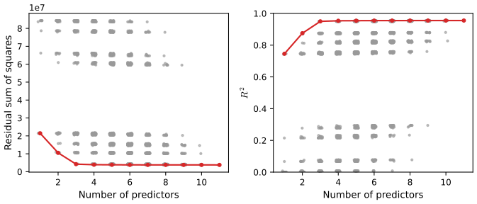
Result 6.1 (counting models; the best RSS never increases with size) Sections 6.1.1–6.1.2
(a) Best subset selection fits \(\sum_{k=0}^p\binom pk=2^p\) models; forward and backward stepwise selection each fit \(1+p(p+1)/2\). For \(p=20\): 1,048,576 against 211; for the Hitters data (\(p=19\)): 524,288 against 191. (b) If \(\RSS_k\) is the smallest RSS among models with \(k\) predictors, then \(\RSS_0\ge\RSS_1\ge\dots\ge\RSS_p\), and the same holds along any forward or backward path.
Filling the gap 6.1: the counts, and why adding a variable cannot increase the RSS Sections 6.1.1–6.1.2
Derivation
(a) Counts. Every subset of the \(p\) predictors is one model, and a set of \(p\) elements has \(2^p\) subsets (each predictor is in or out); grouping by size, \(\sum_k\binom pk=2^p\) by the binomial theorem with \((1+1)^p\). Forward selection fits the null model, then at step \(k=0,1,\dots,p-1\) the \(p-k\) models that add one of the remaining predictors: \[ 1+\sum_{k=0}^{p-1}(p-k)=1+(p+(p-1)+\dots+1)=1+\frac{p(p+1)}{2}. \] Backward selection fits the full model, then at the step from \(k\) to \(k-1\) predictors the \(k\) models that drop one: \(1+\sum_{k=1}^pk\), the same number.
(b) Monotone RSS. Least squares on a set \(S\) of predictors minimises \(\RSS\) over all coefficient vectors that are zero outside \(S\). If \(S\subset S'\), every candidate for \(S\) is also a candidate for \(S'\) (set the extra coefficients to zero), so the minimum over the larger set is no larger: \(\RSS(S')\le\RSS(S)\). Hence \(\RSS_{k+1}\le\RSS(\mathcal M_k\cup\{j\})\le\RSS(\mathcal M_k)=\RSS_k\) for any \(j\). Equivalently \(R^2=1-\RSS/\TSS\) never decreases. This is why step 3 of Algorithm 6.1 cannot use training RSS or \(R^2\). ∎
Best subset selection becomes infeasible for \(p\) beyond about 40 (branch-and-bound methods such as leaps and bounds help, but only for least squares), and the huge search space also invites overfitting: among millions of models some will look good on the training data by chance.
6.1.2 Stepwise Selection
Algorithm 6.2 (forward stepwise selection) Section 6.1.2
- Start from the null model \(\mathcal M_0\).
- For \(k=0,\dots,p-1\): among the \(p-k\) models that add one predictor to \(\mathcal M_k\), call the one with the smallest RSS \(\mathcal M_{k+1}\).
- Choose one of \(\mathcal M_0,\dots,\mathcal M_p\) by cross-validation, \(C_p\) (AIC), BIC or adjusted \(R^2\).
Algorithm 6.3 (backward stepwise selection) Section 6.1.2
- Start from the full model \(\mathcal M_p\) (this needs \(n>p\)).
- For \(k=p,p-1,\dots,1\): among the \(k\) models that drop one predictor from \(\mathcal M_k\), call the one with the smallest RSS \(\mathcal M_{k-1}\).
- Choose one of \(\mathcal M_0,\dots,\mathcal M_p\) as in Algorithm 6.2.
Both are greedy: they give nested sequences of models and are not guaranteed to find the best model of each size. Forward selection can be used even when \(p\gt n\) (it stops at \(\mathcal M_{n-1}\)); backward selection cannot. Hybrid methods add variables like forward selection but may also drop variables that no longer help.
Table 6.1. The first four models of best subset, forward and backward selection on the Credit data Section 6.1.2
| Size | Best subset | Forward stepwise | Backward stepwise |
|---|---|---|---|
| 1 | Rating | Rating | Limit |
| 2 | Rating, Income | Rating, Income | Limit, Income |
| 3 | Rating, Income, Student | Rating, Income, Student | Limit, Income, Student |
| 4 | Cards, Income, Student, Limit | Rating, Income, Student, Limit | Cards, Income, Student, Limit |
The first two columns reproduce the book's Table 6.1 exactly. The third column (not in the book) shows that backward selection, which starts from the full model and therefore keeps Limit rather than its near-copy Rating (correlation 0.997), reaches the best four-variable model but not the best one-, two- or three-variable models. Each stepwise method fitted 67 models here, against 2048 for best subset.
6.1.3 Choosing the Optimal Model
To choose among models of different sizes we need an estimate of test error. Either we adjust the training error for the size of the model (\(C_p\), AIC, BIC, adjusted \(R^2\)), or we estimate the test error directly by a validation set or cross-validation (Chapter 5).
Definition 6.1 (\(C_p\), AIC, BIC and adjusted \(R^2\)) Section 6.1.3, (6.2)–(6.4)
For a least squares model with \(d\) predictors, residual sum of squares \(\RSS\), and \(\hat\sigma^2\) an estimate of \(\Var(\epsilon)\) (usually from the full model, \(\hat\sigma^2=\RSS_{\rm full}/(n-p-1)\)):
\[ C_p=\frac1n\big(\RSS+2d\hat\sigma^2\big), \tag{6.2} \] \[ \BIC=\frac1n\big(\RSS+\log(n)\,d\hat\sigma^2\big), \tag{6.3} \] \[ \text{Adjusted }R^2=1-\frac{\RSS/(n-d-1)}{\TSS/(n-1)}. \tag{6.4} \]For the Gaussian linear model \(\AIC\) is proportional to \(C_p\) (Filling the gap 6.3). Small \(C_p\), AIC and BIC, and large adjusted \(R^2\), are good. Since \(\log n\gt2\) once \(n\ge8\), BIC penalises each extra variable more heavily than \(C_p\) and tends to choose smaller models. (Mallows' original \(C'_p=\RSS/\hat\sigma^2+2d-n\) satisfies \(C_p=\hat\sigma^2(C'_p+n)/n\), so it ranks models in the same order.)
Result 6.2 (\(C_p\) estimates the test error without bias) Section 6.1.3, "beyond the scope of this book"
Assume \(y_i=f(x_i)+\epsilon_i\) with independent errors of variance \(\sigma^2\), fix the inputs, and let \(\hat y_i\) be the least squares fit of a model with \(d\) predictors and an intercept chosen without looking at \(\by\). If \(\by^{\rm new}\) are new responses at the same inputs, then \[ \E\Big[\frac1n\sum_i(y_i^{\rm new}-\hat y_i)^2\Big]=\E\Big[\frac{\RSS}n\Big]+\frac{2(d+1)\sigma^2}n. \] So \((\RSS+2d\hat\sigma^2)/n\) with an unbiased \(\hat\sigma^2\) estimates the test MSE without bias, up to the constant \(2\sigma^2/n\), which is the same for every model.
Filling the gap 6.2: where the penalty \(2d\hat\sigma^2\) comes from Section 6.1.3
Derivation
Write the fit as \(\hat\by=\bH\by\), where \(\bH\) is the projection onto the column space of the \(n\times(d+1)\) design (ones and the \(d\) predictors). \(\bH\) is symmetric, \(\bH^2=\bH\), and \(\tr\bH=d+1\). With \(\by=\bf+\be\):
Training error. \(\by-\hat\by=(\bI-\bH)\by\), so \(\RSS=\|(\bI-\bH)\bf\|^2+2\bf^\T(\bI-\bH)\be+\be^\T(\bI-\bH)\be\). The middle term has mean 0, and \(\E[\be^\T\bA\be]=\sigma^2\tr\bA\) for any fixed matrix \(\bA\) (expand the quadratic form: only the diagonal terms survive). Hence \[ \E[\RSS]=\|(\bI-\bH)\bf\|^2+\sigma^2(n-d-1). \]
Test error at the same inputs. \(\by^{\rm new}-\hat\by=(\bf-\bH\bf)+\be^{\rm new}-\bH\be\), and the three pieces are uncorrelated (the new errors are independent of the old). So \[ \E\|\by^{\rm new}-\hat\by\|^2=\|(\bI-\bH)\bf\|^2+n\sigma^2+\sigma^2\tr(\bH\bH^\T)=\|(\bI-\bH)\bf\|^2+\sigma^2(n+d+1). \]
The difference is \(\sigma^2(n+d+1)-\sigma^2(n-d-1)=2(d+1)\sigma^2\): the training RSS is too small, on average, by twice the number of parameters times \(\sigma^2\). This gap, the optimism of the training error, grows with \(d\), which is exactly why training RSS always favours the largest model. Adding the estimated optimism \(2d\hat\sigma^2\) (dropping the common \(2\sigma^2\) for the intercept) gives (6.2). The argument needs the model to be fixed in advance: after a search over many models, the RSS of the winner is biased further downwards, so \(C_p\) of a selected model is optimistic too. ∎
Result 6.3 (for least squares, AIC is \(C_p\), and BIC is \(C_p\) with \(2\) replaced by \(\log n\)) Section 6.1.3, "irrelevant constants omitted"
For the linear model with Gaussian errors and \(\sigma^2\) replaced by the full-model \(\hat\sigma^2\), AIC and BIC are increasing affine functions of (6.2) and (6.3), so AIC and \(C_p\) always choose the same model. When \(\sigma^2\) is instead estimated within each model, \(\AIC=n\log(\RSS/n)+2d\) and \(\BIC=n\log(\RSS/n)+d\log n\), up to constants.
Filling the gap 6.3: AIC and BIC for the linear model, and the two forms of AIC Section 6.1.3 and its footnote 4
Derivation
With Gaussian errors the log-likelihood of a model with \(d\) predictors is \[ \ell(\bb,\sigma^2)=-\frac n2\log(2\pi\sigma^2)-\frac{\RSS(\bb)}{2\sigma^2}, \] maximised over \(\bb\) by least squares. AIC is \(-2\ell_{\max}+2\times(\text{number of parameters})\) and BIC is \(-2\ell_{\max}+\log(n)\times(\text{number of parameters})\).
\(\sigma^2\) known (in practice replaced by \(\hat\sigma^2\) from the full model): \(-2\ell_{\max}=n\log(2\pi\sigma^2)+\RSS/\sigma^2\), so \[ \AIC=\frac{\RSS+2d\sigma^2}{\sigma^2}+\text{const},\qquad \BIC=\frac{\RSS+\log(n)\,d\sigma^2}{\sigma^2}+\text{const}, \] where the constants do not depend on the model. Multiplying by \(\sigma^2/n\) does not change which model is smallest, and gives (6.2) and (6.3): for least squares AIC and \(C_p\) choose the same model.
\(\sigma^2\) unknown (estimated by maximum likelihood within each model, \(\hat\sigma^2_d=\RSS/n\)): \(-2\ell_{\max}=n\log(\RSS/n)+n+n\log2\pi\), so \[ \AIC=n\log(\RSS/n)+2d+\text{const},\qquad \BIC=n\log(\RSS/n)+d\log n+\text{const}. \] This is the "log(RSS)" form of the footnote, and the BIC that R's leaps reports (it uses \(n\log(\RSS/\TSS)+(d+1)\log n\), which differs by a constant). The two forms can choose different models, because the second estimates \(\sigma^2\) afresh in each model.
Why \(\log n\)? BIC approximates \(-2\log\) of the marginal likelihood of a model, \(\int L(\bb)\pi(\bb)\,d\bb\). Around the maximum the likelihood is approximately Gaussian with a covariance of order \(1/n\) in each of the \(d\) directions, so the integral is about \(L_{\max}\times(\text{const}/n)^{d/2}\); taking \(-2\log\) gives \(-2\ell_{\max}+d\log n+O(1)\) (the Laplace approximation). ∎
Result 6.4 (what adjusted \(R^2\) rewards) Section 6.1.3
Maximising adjusted \(R^2\) is the same as minimising \(\RSS/(n-d-1)\), the usual unbiased estimate of \(\sigma^2\) in the \(d\)-variable model. Adding one predictor to a model raises adjusted \(R^2\) if and only if the \(F\) statistic for that predictor (the square of its \(t\) statistic) exceeds 1.
Filling the gap 6.4: adjusted \(R^2\) and the \(F\) statistic Section 6.1.3
Derivation
\(\TSS/(n-1)\) is the same for every model, so (6.4) is largest when \(\RSS/(n-d-1)\) is smallest. Now add one predictor to a \(d\)-variable model, lowering the RSS from \(\RSS_0\) to \(\RSS_1\). The \(F\) statistic for the new predictor is \(F=(\RSS_0-\RSS_1)/\big(\RSS_1/(n-d-2)\big)\), and it equals the square of the predictor's \(t\) statistic. Adjusted \(R^2\) rises iff \[ \frac{\RSS_1}{n-d-2}\lt\frac{\RSS_0}{n-d-1}\iff (n-d-1)\RSS_1\lt(n-d-2)\RSS_0\iff \RSS_1\lt(n-d-2)(\RSS_0-\RSS_1)\iff F\gt1. \] So adjusted \(R^2\) keeps any variable with \(|t|\gt1\), a much weaker requirement than the usual \(|t|\gt2\); this is why it tends to choose larger models than \(C_p\) (which corresponds roughly to \(|t|\gt\sqrt2\)) and BIC (\(|t|\gt\sqrt{\log n}\)). ∎
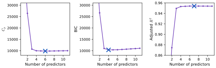
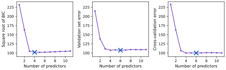
Validation and cross-validation. The direct approach computes, for each size \(d\), the validation-set or \(k\)-fold cross-validation error of the best \(d\)-variable model, the selection being redone on each training part. It makes fewer assumptions (no \(\hat\sigma^2\), no need to count parameters) and is cheap on modern computers. With curves as flat as these, the one-standard-error rule is sensible: take the smallest model whose estimated error is within one standard error of the minimum.
6.2 Shrinkage Methods
Instead of choosing a subset, fit all \(p\) predictors but penalise the size of the coefficients. It is not obvious that a constraint should improve the fit; the point is that shrinking the estimates towards zero can reduce their variance a lot while adding only a little bias.
6.2.1 Ridge Regression
Definition 6.2 (ridge regression) Section 6.2.1, (6.5)
For a tuning parameter \(\lambda\ge0\), the ridge estimates \(\hb^R_\lambda\) minimise
\[ \sum_{i=1}^n\Big(y_i-\beta_0-\sum_{j=1}^p\beta_jx_{ij}\Big)^2+\lambda\sum_{j=1}^p\beta_j^2=\RSS+\lambda\sum_{j=1}^p\beta_j^2. \tag{6.5} \]The shrinkage penalty \(\lambda\sum_j\beta_j^2\) does not include the intercept. \(\lambda=0\) gives least squares; \(\lambda\to\infty\) gives the null model. Each \(\lambda\) gives a different fit, so \(\lambda\) has to be chosen (Section 6.2.3).
Result 6.5 (the ridge solution) Section 6.2.1
Centre the predictors (and keep them centred from now on). Then the ridge intercept is \(\hat\beta_0=\bar y\) and the slopes are \[ \hb^R_\lambda=(\bX^\T\bX+\lambda\bI)^{-1}\bX^\T\by, \] which exists and is unique for every \(\lambda\gt0\), even when \(p\gt n\) or the predictors are collinear. With the singular value decomposition \(\bX=\bU\bD\bV^\T\) (singular values \(d_1\ge\dots\ge d_p\)), the fitted values are \(\hat\by=\bar y\bone+\sum_j\bu_j\frac{d_j^2}{d_j^2+\lambda}\bu_j^\T\by\): ridge shrinks the component of \(\by\) along the \(j\)th principal direction by the factor \(d_j^2/(d_j^2+\lambda)\), most where the predictors vary least.
Filling the gap 6.5: solving (6.5) Section 6.2.1, "the estimated intercept will take the form \(\bar y\)"
Derivation
Intercept. With centred columns, \(\sum_ix_{ij}=0\). The derivative of (6.5) with respect to \(\beta_0\) is \(-2\sum_i(y_i-\beta_0-\sum_j\beta_jx_{ij})=-2(n\bar y-n\beta_0)\), because the \(x\) terms sum to zero. It vanishes at \(\beta_0=\bar y\) whatever the slopes, so \(\hat\beta_0=\bar y\), and the slopes minimise \(\|\by-\bar y\bone-\bX\bb\|^2+\lambda\|\bb\|^2\). Since \(\bX^\T\bone=\mathbf 0\), we may replace \(\by-\bar y\bone\) by \(\by\) in what follows.
Slopes. The gradient of \(\|\by-\bX\bb\|^2+\lambda\bb^\T\bb\) is \(-2\bX^\T(\by-\bX\bb)+2\lambda\bb\); setting it to zero gives \((\bX^\T\bX+\lambda\bI)\bb=\bX^\T\by\). For any \(\ba\ne\mathbf0\), \(\ba^\T(\bX^\T\bX+\lambda\bI)\ba=\|\bX\ba\|^2+\lambda\|\ba\|^2\gt0\) when \(\lambda\gt0\), so the matrix is positive definite: invertible, and the criterion is strictly convex, so this stationary point is the unique minimiser. (For least squares, \(\lambda=0\), the matrix \(\bX^\T\bX\) is singular when \(p\ge n\): see Result 6.15.)
SVD form. \(\bX^\T\bX=\bV\bD^2\bV^\T\) and \(\bX^\T\bX+\lambda\bI=\bV(\bD^2+\lambda\bI)\bV^\T\), so \(\hb^R_\lambda=\bV(\bD^2+\lambda\bI)^{-1}\bD\bU^\T\by=\sum_j\bv_j\frac{d_j}{d_j^2+\lambda}\bu_j^\T\by\) and \(\bX\hb^R_\lambda=\sum_j\bu_j\frac{d_j^2}{d_j^2+\lambda}\bu_j^\T\by\). Each factor lies in \([0,1)\) and decreases in \(\lambda\), so \(\|\hb^R_\lambda\|_2\) decreases steadily from the least squares norm to 0, as the book states for the right-hand panel of Figure 6.4. ∎
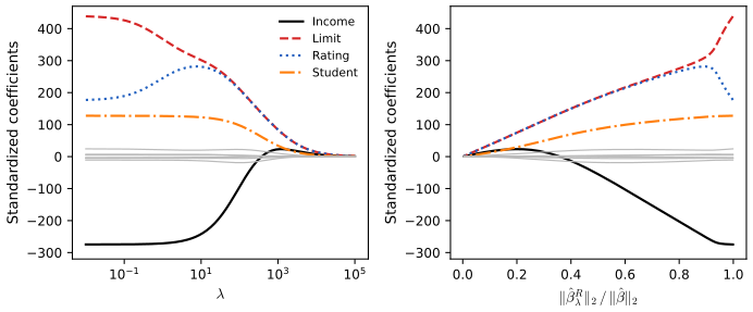
Standardise first. Least squares is scale equivariant: measuring income in thousands of dollars multiplies its coefficient by 1000 and leaves the fit unchanged. Ridge regression is not, because the penalty treats all coefficients alike. It is therefore applied to predictors standardised to standard deviation one,
\[ \tilde x_{ij}=\frac{x_{ij}}{\sqrt{\frac1n\sum_{i=1}^n(x_{ij}-\bar x_j)^2}}, \tag{6.6} \]and the "standardised coefficients" of Figure 6.4 are the coefficients of the \(\tilde x_j\). (glmnet in R standardises internally and reports coefficients on the original scale; in scikit-learn the scaling is an explicit pipeline step. The lab uses both.)
Result 6.6 (ridge depends on the units of the predictors) Section 6.2.1
Replace \(x_j\) by \(cx_j\). Least squares then gives \(\hat\beta_j/c\) and the same fitted values. Ridge regression with the same \(\lambda\) gives the coefficient that the original problem would give with the penalty on \(\beta_j\) changed from \(\lambda\) to \(\lambda/c^2\): a different fit, in which \(\beta_j\) is penalised less if \(c\gt1\), and every other coefficient changes too.
Filling the gap 6.6: why units matter for ridge and not for least squares Section 6.2.1
Derivation
Let \(\bX'=\bX\bS\) with \(\bS=\diag(1,\dots,c,\dots,1)\) (\(c\) in position \(j\)). For any \(\bb'\), \(\bX'\bb'=\bX(\bS\bb')\), so fitting with \(\bX'\) and coefficients \(\bb'\) is fitting with \(\bX\) and \(\bb=\bS\bb'\). Least squares minimises \(\|\by-\bX'\bb'\|^2=\|\by-\bX\bb\|^2\) over all \(\bb'\), i.e. over all \(\bb\): same minimiser \(\hb\), hence \(\hat\beta'_j=\hat\beta_j/c\) and the same fit. Ridge minimises \(\|\by-\bX\bb\|^2+\lambda\|\bS^{-1}\bb\|^2=\|\by-\bX\bb\|^2+\lambda\sum_{k\ne j}\beta_k^2+(\lambda/c^2)\beta_j^2\): a different penalty, so a different solution, and because the normal equations couple all coefficients, the others move as well. After standardisation (6.6) every column has the same scale, so the choice of units no longer matters. Confirmed numerically on the Hitters data: measuring one column in different units changes the ridge fit on the raw columns and leaves the fit on standardised columns unchanged. ∎
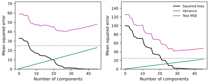
Why ridge can beat least squares. As \(\lambda\) grows the fit becomes less flexible: variance falls and bias rises. Figure 6.5 shows this on a simulation like the book's, with \(n=50\) observations and \(p=45\) predictors that all affect the response.
Result 6.7 (bias and variance of ridge at the training inputs) Section 6.2.1, Figure 6.5
Let \(\by=\bf+\be\) with fixed inputs, \(\E\be=\mathbf0\), \(\Var\be=\sigma^2\bI\), and \(\bf\) centred for simplicity. Then the ridge fit \(\hat\by=\bar y\bone+\bH_\lambda\by\), \(\bH_\lambda=\sum_j\frac{d_j^2}{d_j^2+\lambda}\bu_j\bu_j^\T\), has, averaged over the \(n\) training inputs, \[ \text{squared bias}=\frac1n\sum_j\Big(\frac{\lambda}{d_j^2+\lambda}\Big)^2(\bu_j^\T\bf)^2+\frac1n\|\bf_\perp\|^2,\qquad \text{variance}=\frac{\sigma^2}n\Big(1+\sum_j\Big(\frac{d_j^2}{d_j^2+\lambda}\Big)^2\Big), \] where \(\bf_\perp\) is the part of \(\bf\) outside the column space of \(\bX\). The squared bias increases and the variance decreases with \(\lambda\); at \(\lambda=0\) the variance is \(\sigma^2(p+1)/n\), which for \(p=45\), \(n=50\) is 92% of \(\sigma^2\).
Filling the gap 6.7: computing the curves of Figure 6.5 Section 6.2.1
Derivation
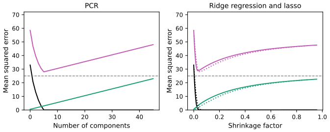
\(\E\hat\by=\bar f\bone+\bH_\lambda\bf\) because \(\E\bar y=\bar f\) and \(\bH_\lambda\) is fixed. The bias vector is \(\bf-\E\hat\by=(\bI-\bH_\lambda)\bf\) (with \(\bar f=0\)); expanding \(\bf\) in the orthonormal basis \(\bu_1,\dots,\bu_p\) plus the orthogonal remainder gives the first formula, since \((\bI-\bH_\lambda)\bu_j=\frac{\lambda}{d_j^2+\lambda}\bu_j\). The fit is linear in \(\by\): \(\hat\by=(\frac1n\bone\bone^\T+\bH_\lambda)\by\), so its covariance is \(\sigma^2\bA\bA^\T\) with \(\bA=\frac1n\bone\bone^\T+\bH_\lambda\). The two parts are orthogonal projections-like pieces acting on orthogonal subspaces (\(\bH_\lambda\bone=\mathbf0\) because \(\bX\) is centred), so \(\tr(\bA\bA^\T)=1+\sum_j(d_j^2/(d_j^2+\lambda))^2\). The expected test MSE at the training inputs is \(\sigma^2+\text{squared bias}+\text{variance}\), as in Chapter 2. These are the exact formulas behind Figures 6.5, 6.18 and 6.19 (PCR uses factors 1 for \(j\le M\) and 0 otherwise); for the lasso, which is not linear in \(\by\), the code averages over 400 simulated response vectors. ∎
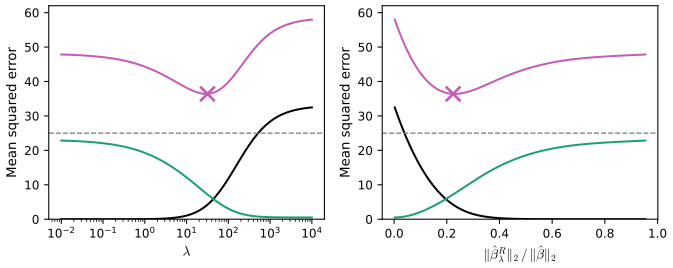
Ridge therefore works best where least squares has high variance: \(p\) close to \(n\), or \(p\gt n\). It is also cheap: one fit per \(\lambda\), and the whole path costs about as much as one least squares fit (one SVD).
6.2.2 The Lasso
Definition 6.3 (the lasso) Section 6.2.2, (6.7)
The lasso estimates \(\hb^L_\lambda\) minimise
\[ \sum_{i=1}^n\Big(y_i-\beta_0-\sum_{j=1}^p\beta_jx_{ij}\Big)^2+\lambda\sum_{j=1}^p|\beta_j|=\RSS+\lambda\sum_{j=1}^p|\beta_j|. \tag{6.7} \]The only change from ridge is the \(\ell_1\) penalty \(\lambda\|\bb\|_1\) in place of the \(\ell_2\) penalty. For \(\lambda\) large enough some coefficients are exactly zero, so the lasso performs variable selection and gives sparse models.
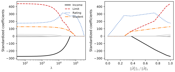
Another formulation. For every \(\lambda\) there is a budget \(s\) such that the lasso and ridge solve, respectively,
\[ \underset{\bb}{\text{minimize}}\ \sum_{i=1}^n\Big(y_i-\beta_0-\sum_{j=1}^p\beta_jx_{ij}\Big)^2\quad\text{subject to}\quad\sum_{j=1}^p|\beta_j|\le s, \tag{6.8} \] \[ \underset{\bb}{\text{minimize}}\ \sum_{i=1}^n\Big(y_i-\beta_0-\sum_{j=1}^p\beta_jx_{ij}\Big)^2\quad\text{subject to}\quad\sum_{j=1}^p\beta_j^2\le s, \tag{6.9} \]and best subset selection of size \(s\) is
\[ \underset{\bb}{\text{minimize}}\ \sum_{i=1}^n\Big(y_i-\beta_0-\sum_{j=1}^p\beta_jx_{ij}\Big)^2\quad\text{subject to}\quad\sum_{j=1}^pI(\beta_j\ne0)\le s. \tag{6.10} \]So ridge and the lasso are computationally feasible relatives of best subset, with the intractable count of nonzero coefficients replaced by a convex budget; the lasso, whose budget also produces zeros, is the closer relative.
Result 6.8 (penalty and budget are two views of the same estimates) Section 6.2.2, "one can show"
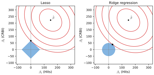
(a) If \(\hb_\lambda\) minimises \(\RSS+\lambda P(\bb)\) with \(\lambda\gt0\) and \(P=\|\cdot\|_1\) or \(\|\cdot\|_2^2\), then \(\hb_\lambda\) also solves "minimise RSS subject to \(P(\bb)\le s\)" with \(s=P(\hb_\lambda)\). (b) Conversely, if \(s\) is smaller than \(P\) of the least squares estimate, the constrained solution lies on the boundary \(P(\bb)=s\) and solves the penalised problem for some \(\lambda\gt0\). (c) Geometrically, the constrained solution is the first point where the elliptical contours of the RSS around \(\hb\) touch the constraint region. The \(\ell_1\) region (a diamond for \(p=2\), a polytope in general) has corners on the axes, so the contact point often has some coordinates exactly 0; the \(\ell_2\) region (a disc, a sphere) has no corners, so contact on an axis happens only by accident.
Filling the gap 6.8: from penalty to budget and back Section 6.2.2
Derivation
(a) Let \(s=P(\hb_\lambda)\) and suppose some \(\bb\) with \(P(\bb)\le s\) had \(\RSS(\bb)\lt\RSS(\hb_\lambda)\). Then \(\RSS(\bb)+\lambda P(\bb)\lt\RSS(\hb_\lambda)+\lambda P(\hb_\lambda)\), contradicting the optimality of \(\hb_\lambda\). So \(\hb_\lambda\) is the constrained minimiser.
(b) If the constrained minimiser \(\bb^*\) were strictly inside the region, it would be a local, hence (by convexity of RSS) global, minimiser of the RSS, i.e. a least squares solution, impossible when \(s\lt P(\hb)\). So \(P(\bb^*)=s\). Both RSS and \(P\) are convex, and the region \(P\le s\) contains points with \(P\lt s\) (e.g. \(\mathbf0\)), so convex duality (the Lagrange multiplier theorem; Slater's condition holds) gives a multiplier \(\lambda\ge0\) with \(\bb^*\) minimising \(\RSS+\lambda(P(\bb)-s)\); \(\lambda=0\) would again make \(\bb^*\) a least squares solution, so \(\lambda\gt0\). For differentiable \(P\) (ridge) this is the familiar condition that the gradients are parallel: \(\nabla\RSS(\bb^*)=-\lambda\nabla P(\bb^*)\).
(c) With \(\bX\) of full rank, \(\RSS(\bb)=\RSS(\hb)+(\bb-\hb)^\T\bX^\T\bX(\bb-\hb)\) (expand around the least squares solution; the cross term vanishes by the normal equations). Its level sets are ellipses centred at \(\hb\). Growing the ellipse until it first meets the region \(P\le s\) gives the constrained minimiser. A corner of the diamond is a point where the boundary is not smooth; an ellipse can touch it there from a whole range of directions (the "normal cone" of the corner), so landing on a corner is not a coincidence but happens for an open set of positions of \(\hb\). The disc has a single normal direction at each point, so landing exactly on an axis requires \(\hb\) to lie on a particular line. ∎
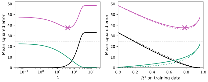
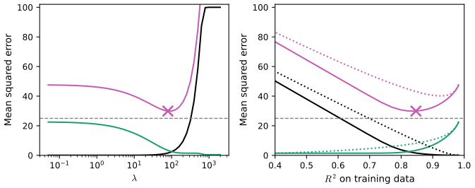
Comparing the lasso and ridge. Neither dominates. On the simulation of Figure 6.5, where all 45 coefficients are nonzero, ridge is slightly better (Figure 6.8); when only two predictors matter, the lasso is clearly better (Figure 6.9). Plotting against training \(R^2\) puts the two methods on a common axis. In practice the truth is unknown and cross-validation decides.
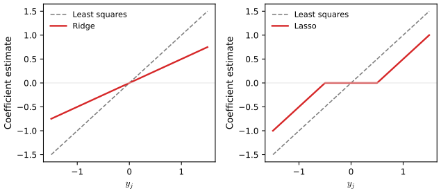
A simple special case. Take \(n=p\), \(\bX=\bI\) and no intercept. Least squares minimises \(\sum_{j=1}^p(y_j-\beta_j)^2\), so \(\hat\beta_j=y_j\); ridge and the lasso minimise
\[ \sum_{j=1}^p(y_j-\beta_j)^2 \tag{6.11} \] \[ \sum_{j=1}^p(y_j-\beta_j)^2+\lambda\sum_{j=1}^p\beta_j^2, \tag{6.12} \] \[ \sum_{j=1}^p(y_j-\beta_j)^2+\lambda\sum_{j=1}^p|\beta_j| \tag{6.13} \]respectively ((6.11) is least squares), and the solutions are
\[ \hat\beta^R_j=\frac{y_j}{1+\lambda}, \tag{6.14} \] \[ \hat\beta^L_j=\begin{cases}y_j-\lambda/2&\text{if }y_j\gt\lambda/2,\\ y_j+\lambda/2&\text{if }y_j\lt-\lambda/2,\\ 0&\text{if }|y_j|\le\lambda/2.\end{cases} \tag{6.15} \]Result 6.9 (proportional shrinkage, soft thresholding, hard thresholding) Section 6.2.2, "one can show"
With \(\bX=\bI\): (a) ridge is (6.14), every estimate shrunk by the same factor; (b) the lasso is (6.15), \(\hat\beta^L_j=\sign(y_j)(|y_j|-\lambda/2)_+\), every estimate moved towards zero by the same amount \(\lambda/2\) and set to zero when it would cross it (soft thresholding); (c) best subset with the penalty \(\lambda\sum_jI(\beta_j\ne0)\) keeps \(\hat\beta_j=y_j\) when \(|y_j|\gt\sqrt\lambda\) and sets it to 0 otherwise (hard thresholding).
Filling the gap 6.9: deriving (6.14) and (6.15) Section 6.2.2
Derivation
All three criteria are sums of separate terms, one per \(j\), so each \(\beta_j\) can be minimised on its own. Write \(y=y_j\), \(b=\beta_j\).
(a) Ridge. \(g(b)=(y-b)^2+\lambda b^2\) has \(g'(b)=-2(y-b)+2\lambda b=0\iff b=y/(1+\lambda)\), and \(g''=2(1+\lambda)\gt0\): (6.14).
(b) Lasso. \(h(b)=(y-b)^2+\lambda|b|\) is convex but not differentiable at 0. On \(b\gt0\), \(h'(b)=-2(y-b)+\lambda\), zero at \(b=y-\lambda/2\), which is a valid positive point only if \(y\gt\lambda/2\). On \(b\lt0\), \(h'(b)=-2(y-b)-\lambda\), zero at \(b=y+\lambda/2\), valid only if \(y\lt-\lambda/2\). If \(|y|\le\lambda/2\), then for \(b\gt0\), \(h'(b)=2b+(\lambda-2y)\gt0\), and for \(b\lt0\), \(h'(b)=2b-(\lambda+2y)\lt0\): \(h\) decreases up to 0 and increases after it, so the minimum is at \(b=0\). These three cases are (6.15). (In the language of subgradients: \(0\in-2(y-b)+\lambda\,\partial|b|\), and \(\partial|0|=[-1,1]\) gives \(b=0\) exactly when \(|2y|\le\lambda\).)
(c) Hard thresholding. With \(k(b)=(y-b)^2+\lambda I(b\ne0)\): the best nonzero choice is \(b=y\), costing \(\lambda\); the choice \(b=0\) costs \(y^2\). So keep \(y\) iff \(y^2\gt\lambda\). Unlike (b), the estimate jumps from 0 to \(\sqrt\lambda\) at the threshold and is not shrunk beyond it.
For a general \(\bX\) the story is only approximately the same: ridge roughly shrinks each principal direction by a fixed factor, and the lasso roughly moves the coefficients towards zero by a similar amount, zeroing the small ones. ∎
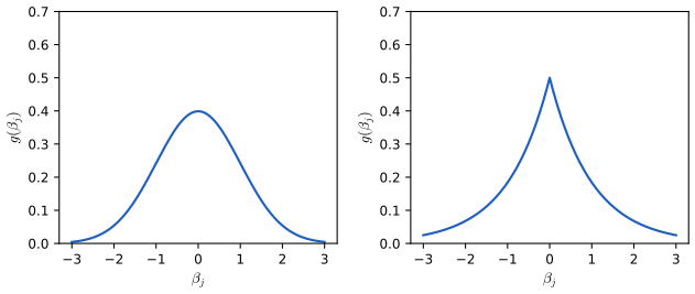
Bayesian interpretation. Give \(\bb\) a prior \(p(\bb)=\prod_jg(\beta_j)\) and assume Gaussian errors. The posterior is \(p(\bb\given\bX,\bY)\propto f(\bY\given\bX,\bb)p(\bb)\), and its mode is the most probable coefficient vector given the data.
Result 6.10 (ridge and the lasso are posterior modes) Section 6.2.2; Exercise 7
With \(y_i=\beta_0+\sum_jx_{ij}\beta_j+\epsilon_i\), \(\epsilon_i\sim\N(0,\sigma^2)\) independent, and a flat prior on \(\beta_0\): (a) if \(g\) is the \(\N(0,c)\) density, the posterior mode and the posterior mean are the ridge estimate with \(\lambda=\sigma^2/c\); (b) if \(g(\beta)=\frac1{2b}e^{-|\beta|/b}\) (the Laplace or double-exponential density), the posterior mode is the lasso estimate with \(\lambda=2\sigma^2/b\); its posterior mean is a different, never sparse, estimate. A small prior variance (small \(c\) or \(b\)) means a large \(\lambda\).
Filling the gap 6.10: the posterior computations Section 6.2.2, "it follows that"
Derivation
Likelihood. \(f(\by\given\bX,\bb)=(2\pi\sigma^2)^{-n/2}\exp\{-\RSS(\bb)/(2\sigma^2)\}\).
(a) Gaussian prior. \(-\log p(\bb\given\by)=\frac{\RSS(\bb)}{2\sigma^2}+\frac{1}{2c}\sum_j\beta_j^2+\text{const}=\frac1{2\sigma^2}\Big(\RSS(\bb)+\frac{\sigma^2}{c}\sum_j\beta_j^2\Big)+\text{const}\). Minimising this is (6.5) with \(\lambda=\sigma^2/c\), so the mode is the ridge estimate. The exponent is a quadratic function of \(\bb\), so the posterior is Gaussian: completing the square, \(\bb\given\by\sim\N\big((\bX^\T\bX+\lambda\bI)^{-1}\bX^\T\by,\ \sigma^2(\bX^\T\bX+\lambda\bI)^{-1}\big)\) (centred \(\bX\), slopes only). A Gaussian's mean equals its mode, so the ridge estimate is also the posterior mean.
(b) Laplace prior. \(-\log p(\bb\given\by)=\frac{\RSS(\bb)}{2\sigma^2}+\frac1b\sum_j|\beta_j|+\text{const}=\frac1{2\sigma^2}\Big(\RSS(\bb)+\frac{2\sigma^2}{b}\sum_j|\beta_j|\Big)+\text{const}\): the lasso (6.7) with \(\lambda=2\sigma^2/b\).
The lasso's posterior mean is not sparse. In the simplest case \(p=n=1\), \(x=1\), the posterior density of \(\beta\) is proportional to \(\exp\{-(y-\beta)^2/(2\sigma^2)-|\beta|/b\}\), positive everywhere and not symmetric about 0 unless \(y=0\). Its mean is therefore nonzero for every \(y\ne0\), even when \(|y|\le\lambda/2\) and the mode (the lasso) is exactly 0. By numerical integration, with \(\sigma=1\), \(b=1\) (\(\lambda=2\)) and \(y=0.5\), the mode is 0 and the posterior mean is 0.24. The Laplace prior is sharply peaked at 0, which is why its mode sits at 0 so often; the Gaussian prior is smooth at 0, so its mode is never exactly 0. ∎
6.2.3 Selecting the Tuning Parameter
Choose a grid of \(\lambda\) values, compute the cross-validation error for each, take the \(\lambda\) with the smallest error, and refit on all the data with that \(\lambda\). For ridge, leave-one-out cross-validation needs only one fit per \(\lambda\).
Result 6.11 (leave-one-out cross-validation for ridge in one fit) Section 6.2.3, Figure 6.12
Let \(\hat\by=\bS_\lambda\by\) with \(\bS_\lambda=\frac1n\bone\bone^\T+\bX(\bX^\T\bX+\lambda\bI)^{-1}\bX^\T\) (centred, standardised \(\bX\) held fixed). Then the leave-one-out error is \[ \mathrm{CV}_{(n)}(\lambda)=\frac1n\sum_{i=1}^n\Big(\frac{y_i-\hat y_i}{1-S_{\lambda,ii}}\Big)^2, \] the same shortcut as for least squares in Chapter 5, with the ridge "hat" matrix in place of the projection.
Filling the gap 6.11: the leave-one-out shortcut for ridge Section 6.2.3
Derivation
Absorb the intercept by adding a column of ones to \(\bX\) and the matrix \(\bP=\diag(0,\lambda,\dots,\lambda)\) to the penalty, so \(\hb=(\bX^\T\bX+\bP)^{-1}\bX^\T\by\) and \(\bS=\bX(\bX^\T\bX+\bP)^{-1}\bX^\T\) (this equals \(\bS_\lambda\) above because the columns are centred). Write \(\bA=\bX^\T\bX+\bP\). Leaving out observation \(i\) replaces \(\bA\) by \(\bA-\bx_i\bx_i^\T\) and \(\bX^\T\by\) by \(\bX^\T\by-\bx_iy_i\). By the Sherman–Morrison formula, \((\bA-\bx_i\bx_i^\T)^{-1}=\bA^{-1}+\frac{\bA^{-1}\bx_i\bx_i^\T\bA^{-1}}{1-h_i}\) with \(h_i=\bx_i^\T\bA^{-1}\bx_i=S_{ii}\). Multiplying out, the prediction at \(\bx_i\) from the other \(n-1\) points is \[ \hat y_{(-i)}=\bx_i^\T(\bA-\bx_i\bx_i^\T)^{-1}(\bX^\T\by-\bx_iy_i)=\frac{\hat y_i-h_iy_i}{1-h_i}, \] so \(y_i-\hat y_{(-i)}=(y_i-\hat y_i)/(1-h_i)\). (Strictly, glmnet and the book re-standardise inside each fold; holding the standardisation fixed changes the curve very little, and makes the formula exact.) The formula was confirmed numerically against explicit refits. ∎
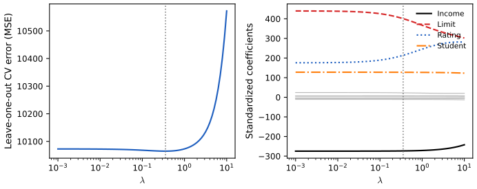
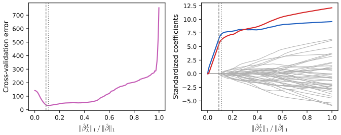
Figure 6.13 shows ten-fold cross-validation for the lasso on one data set from the sparse simulation of Figure 6.9 (\(n=50\), \(p=45\), two signal variables). The minimum of the cross-validation curve is a model whose only nonzero coefficients are the two signal variables: the lasso with cross-validation finds the right variables in a setting with almost as many predictors as observations.
6.3 Dimension Reduction Methods
The third approach transforms the predictors. Let \(Z_1,\dots,Z_M\) (\(M\lt p\)) be linear combinations of the original predictors,
\[ Z_m=\sum_{j=1}^p\phi_{jm}X_j, \tag{6.16} \]and fit by least squares
\[ y_i=\theta_0+\sum_{m=1}^M\theta_mz_{im}+\epsilon_i,\qquad i=1,\dots,n. \tag{6.17} \]Only \(M+1\) coefficients are estimated instead of \(p+1\). The model is still linear in the original predictors:
\[ \sum_{m=1}^M\theta_mz_{im}=\sum_{m=1}^M\theta_m\sum_{j=1}^p\phi_{jm}x_{ij}=\sum_{j=1}^p\Big(\sum_{m=1}^M\theta_m\phi_{jm}\Big)x_{ij}=\sum_{j=1}^p\beta_jx_{ij},\quad\text{where}\quad \beta_j=\sum_{m=1}^M\theta_m\phi_{jm}. \tag{6.18} \](The middle step only exchanges the order of two finite sums.) So dimension reduction is least squares with the coefficient vector \(\bb\) constrained to the \(M\)-dimensional subspace spanned by the direction vectors \(\bphi_1,\dots,\bphi_M\): more bias, less variance. If \(M=p\) and the \(Z_m\) are linearly independent the constraint is empty and we get least squares. The two methods below differ in how they choose the \(\phi_{jm}\).
6.3.1 Principal Components Regression
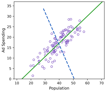
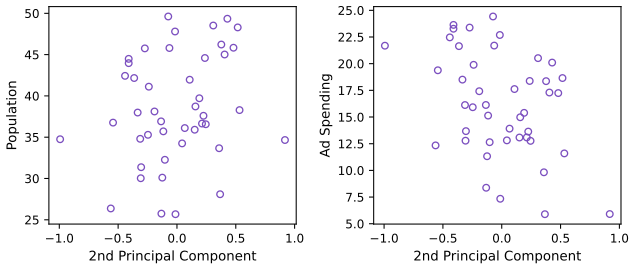
Principal components. The first principal component direction of the data is the direction along which the observations vary most. Figure 6.14 shows it for two predictors, population size (pop, in tens of thousands) and advertising spending (ad, in thousands of dollars) in 100 cities.
For these data the first principal component is
\[ Z_1=0.839\times(\text{pop}-\overline{\text{pop}})+0.544\times(\text{ad}-\overline{\text{ad}}), \tag{6.19} \]and the first principal component scores are
\[ z_{i1}=0.839\times(\text{pop}_i-\overline{\text{pop}})+0.544\times(\text{ad}_i-\overline{\text{ad}}). \tag{6.20} \]The loadings \(\phi_{11}=0.839\), \(\phi_{21}=0.544\) are the direction; they satisfy \(\phi_{11}^2+\phi_{21}^2=1\), without which the variance could be inflated at will. The second principal component \(Z_2=0.544\times(\text{pop}-\overline{\text{pop}})-0.839\times(\text{ad}-\overline{\text{ad}})\) is uncorrelated with \(Z_1\) and has the largest variance among such combinations.
Result 6.12 (what principal components are) Section 6.3.1
Let \(\bX\) be centred, with sample covariance matrix \(\bS=\bX^\T\bX/n\) and eigenvalues \(\ell_1\ge\ell_2\ge\dots\ge\ell_p\ge0\), eigenvectors \(\bv_1,\dots,\bv_p\). (a) Among unit vectors \(\bphi\), the variance of the scores \(\bX\bphi\) is largest for \(\bphi=\bv_1\), and equals \(\ell_1\). (b) The same \(\bv_1\) spans the line that minimises the sum of squared perpendicular distances from the points. (c) Two linear combinations \(\bX\ba\) and \(\bX\bc\) with \(\ba,\bc\) eigenvectors of \(\bS\) are uncorrelated iff \(\ba\perp\bc\); the \(m\)th principal component is \(\bv_m\), the best direction orthogonal to \(\bv_1,\dots,\bv_{m-1}\). (d) The score \(z_{i1}\) is the signed distance along the first direction from the mean to the projection of point \(i\).
Filling the gap 6.12: maximum variance, closest line and orthogonality Section 6.3.1, "it is possible to show"
Derivation
(a) The scores \(\bX\bphi\) have mean 0 and variance \(\bphi^\T\bS\bphi\). Write \(\bphi=\sum_kc_k\bv_k\) in the orthonormal eigenbasis; \(\|\bphi\|=1\) means \(\sum_kc_k^2=1\), and \(\bphi^\T\bS\bphi=\sum_k\ell_kc_k^2\le\ell_1\sum_kc_k^2=\ell_1\), with equality at \(\bphi=\bv_1\). (With a Lagrange multiplier: maximise \(\bphi^\T\bS\bphi-\mu(\bphi^\T\bphi-1)\); the gradient condition \(\bS\bphi=\mu\bphi\) says \(\bphi\) is an eigenvector, and its variance is then \(\mu\), so take the largest eigenvalue.)
(b) For a unit vector \(\bphi\), the projection of the centred point \(\bx_i\) on the line is \((\bx_i^\T\bphi)\bphi\), and by Pythagoras \(\|\bx_i\|^2=(\bx_i^\T\bphi)^2+\text{dist}_i^2\). Summing, \(\sum_i\text{dist}_i^2=\sum_i\|\bx_i\|^2-n\,\bphi^\T\bS\bphi\): the first term does not depend on \(\bphi\), so minimising the distances is maximising the variance. This is also (d): \(z_{i1}=\bx_i^\T\bv_1\) is the coordinate of the projection along the line.
(c) \(\Cov(\bX\ba,\bX\bc)=\ba^\T\bS\bc\). If \(\bc=\bv_k\), this is \(\ell_k\,\ba^\T\bv_k\), zero iff \(\ba\perp\bv_k\) (when \(\ell_k\gt0\)). Restricting \(\bphi\) to be orthogonal to \(\bv_1,\dots,\bv_{m-1}\) forces \(c_1=\dots=c_{m-1}=0\) in (a), and the maximum of \(\sum_{k\ge m}\ell_kc_k^2\) is \(\ell_m\), at \(\bv_m\).
Standardise or not? PCA of standardised variables is PCA of the correlation matrix. For two standardised variables with correlation \(r\gt0\) the correlation matrix \(\begin{pmatrix}1&r\\r&1\end{pmatrix}\) always has eigenvectors \((1,1)/\sqrt2\) and \((1,-1)/\sqrt2\): loadings \(\pm0.707\), whatever the data. So loadings such as 0.839 and 0.544 in (6.19) can only come from unstandardised pop and ad (see Note 3). ∎
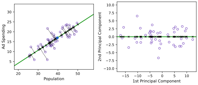
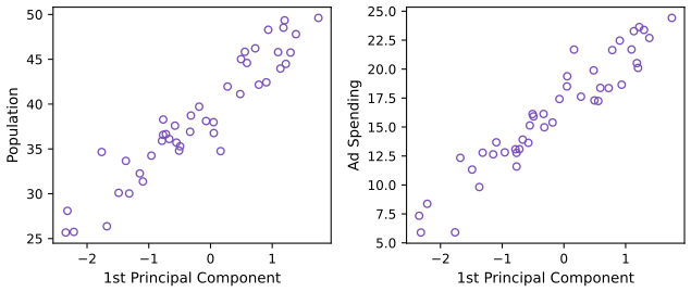
The PCR approach. Principal components regression (PCR) computes the first \(M\) principal components of the (standardised) predictors and regresses \(y\) on them by least squares. The assumption is that the directions in which the predictors vary most are the directions associated with \(Y\). When it holds, PCR estimates \(M\ll p\) coefficients and loses little; when it fails, the useful directions may be among the discarded ones.
Result 6.13 (PCR in coefficient form, and its relation to ridge) Section 6.3.1 and its footnote 7
With \(\bX=\bU\bD\bV^\T\) centred (and standardised), the PCR fit with \(M\) components is \(\hat\by=\bar y\bone+\sum_{j\le M}\bu_j\bu_j^\T\by\), and its coefficients on the original (standardised) predictors are \(\hb^{\rm pcr}_M=\sum_{j\le M}\bv_j\frac{\bu_j^\T\by}{d_j}\). Ridge regression keeps all the components but multiplies the \(j\)th by \(d_j^2/(d_j^2+\lambda)\); PCR multiplies it by 1 for \(j\le M\) and by 0 after. So ridge is a smooth version of PCR, and with \(M=p\) PCR is least squares. PCR is not a variable selection method: every \(\bv_j\) involves all the predictors.
Filling the gap 6.13: deriving the PCR coefficients Section 6.3.1, "one can show that PCR and ridge regression are very closely related"
Derivation
The principal component directions are \(\bv_j\) (the eigenvectors of \(\bX^\T\bX=\bV\bD^2\bV^\T\)), and the score vectors are \(\bz_j=\bX\bv_j=d_j\bu_j\). They are orthogonal, so least squares on \(\bz_1,\dots,\bz_M\) separates into simple regressions: \(\hat\theta_j=\bz_j^\T\by/\bz_j^\T\bz_j=\bu_j^\T\by/d_j\), and the fit is \(\sum_{j\le M}\hat\theta_j\bz_j=\sum_{j\le M}\bu_j\bu_j^\T\by\). By (6.18) with \(\bphi_j=\bv_j\), \(\hb=\sum_{j\le M}\hat\theta_j\bv_j\). Compare Result 6.5: ridge's fit is \(\sum_{j\le p}\frac{d_j^2}{d_j^2+\lambda}\bu_j\bu_j^\T\by\). With \(M=p\) (and full rank) the fit is the projection on the whole column space of \(\bX\), i.e. least squares. The in-sample bias and variance of PCR follow as in Filling the gap 6.7: variance \(\sigma^2(M+1)/n\), squared bias \(\frac1n\sum_{j\gt M}(\bu_j^\T\bf)^2+\frac1n\|\bf_\perp\|^2\). ∎
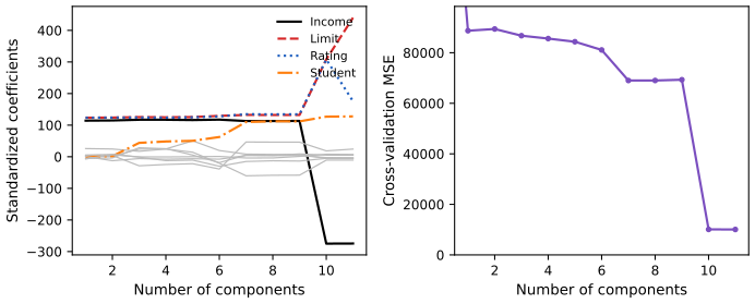
Standardise the predictors before PCR, unless they are all in the same units: otherwise high-variance variables dominate the first components simply because of their units.
6.3.2 Partial Least Squares
PCR chooses its directions without looking at \(Y\) (an unsupervised choice). Partial least squares (PLS) uses the response to choose them: it looks for directions that both summarise the predictors and are related to \(Y\).
Algorithm 6.4 (partial least squares, as described in the book) Section 6.3.2
- Standardise the predictors (and centre \(y\)).
- First direction: set \(\phi_{j1}\) equal to the coefficient of the simple regression of \(Y\) on \(X_j\), \(\phi_{j1}=\langle\bx_j,\by\rangle/\langle\bx_j,\bx_j\rangle\), and \(Z_1=\sum_j\phi_{j1}X_j\).
- For \(m=2,\dots,M\): regress each predictor on \(Z_{m-1}\) and replace it by the residuals; compute \(Z_m\) from these residuals exactly as \(Z_1\) was computed.
- Regress \(y\) on \(Z_1,\dots,Z_M\) by least squares.
Result 6.14 (properties of the PLS directions) Section 6.3.2
(a) For standardised predictors \(\phi_{j1}=\frac{\langle\bx_j,\by\rangle}{n}=\operatorname{sd}(y)\,\Corr(X_j,Y)\): the first direction weights each predictor by its correlation with \(Y\). (b) The PLS components \(Z_1,\dots,Z_M\) are mutually uncorrelated. (c) With \(M=p\) (and \(\bX\) of full rank) PLS is least squares. (d) The first PLS direction explains less variance of the predictors than the first principal component, by (a) of Result 6.12, but is more correlated with \(Y\).
Filling the gap 6.14: why the PLS weights are correlations, and the components uncorrelated Section 6.3.2, "one can show"
Derivation
(a) The simple regression slope of \(y\) on \(x_j\) is \(\sum_i(x_{ij}-\bar x_j)(y_i-\bar y)/\sum_i(x_{ij}-\bar x_j)^2\). For a standardised predictor the denominator is \(n\), so the slope is \(\frac1n\sum_ix_{ij}(y_i-\bar y)=s_y\,r_j\), where \(s_y\) is the (1/n) standard deviation of \(y\) and \(r_j\) the correlation. The factor \(s_y\) is common to all \(j\), so the direction is proportional to the vector of correlations.
(b) After step 3 every residualised predictor is orthogonal to \(Z_1,\dots,Z_{m-1}\) (each regression on \(Z_k\) removes that component, and later steps keep orthogonality because the \(Z\)'s already are). \(Z_m\) is a linear combination of these residuals, so it is orthogonal to (uncorrelated with, all being centred) the earlier components.
(c) By (b) the \(p\) components are orthogonal and, unless the residuals vanish early, nonzero, so they span the column space of \(\bX\): regressing on them is projecting on that space, i.e. least squares. If the residuals become zero before \(M=p\) (or \(Z_m\) becomes 0 because the residual of \(y\) is uncorrelated with all of them), the fit has already reached least squares.
(d) On the simulated cities (Figure 6.21) the first principal direction has slope \(0.544/0.839=0.65\) in the (pop, ad) plane, the first PLS direction (computed on the centred data, so that it can be drawn in the same units) has \(0.508/0.861=0.59\): pop, which correlates 0.88 with sales against 0.75 for ad, gets more weight. ∎
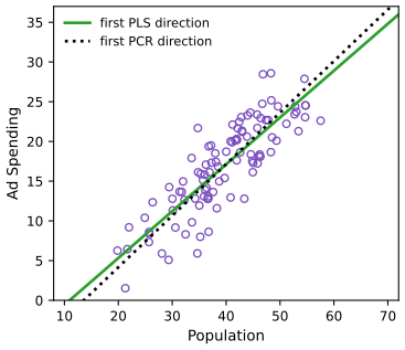
The number of PLS directions \(M\) is chosen by cross-validation. PLS is popular in chemometrics, where spectra give thousands of correlated predictors. In practice it often does no better than ridge or PCR: using \(Y\) to choose the directions reduces bias but adds variance.
6.4 Considerations in High Dimensions
6.4.1 High-Dimensional Data
Most classical methods assume the low-dimensional setting \(n\gg p\). Modern data often have more features than observations: half a million genetic markers (SNPs) for a few hundred patients, or every search term ever typed by a few thousand users (a "bag-of-words" model, in which each term is recorded as present (1) or absent (0)). Data with \(p\gt n\) are called high-dimensional. The dangers discussed below already matter when \(p\) is only slightly smaller than \(n\).
6.4.2 What Goes Wrong in High Dimensions?
Result 6.15 (with \(p+1\ge n\) least squares interpolates) Section 6.4.2
If \(p+1\ge n\) and the \(n\times(p+1)\) design matrix (ones and predictors) has rank \(n\), then for any response vector there are coefficients with zero residuals, so \(\RSS=0\), \(R^2=1\) and training MSE \(=0\), whatever the relationship between \(X\) and \(Y\). Consequences: \(\hat\sigma^2=\RSS/(n-p-1)\) is 0 or undefined, so \(C_p\), AIC and BIC (which need \(\hat\sigma^2\)) break down, and adjusted \(R^2\) can equal 1. With \(p+1\gt n\) the least squares solution is not even unique. Even with \(p\lt n\) and features unrelated to \(Y\), \(\E[R^2]=p/(n-1)\) under Gaussian errors: \(R^2\) rises in proportion to the number of useless features.
Filling the gap 6.15: why the fit becomes perfect, and how fast \(R^2\) grows by chance Section 6.4.2
Derivation
Interpolation. If the design \(\tilde\bX\) (\(n\times(p+1)\)) has rank \(n\), its columns span all of \(\R^n\), so \(\tilde\bX\bb=\by\) has a solution for every \(\by\): the residuals are zero. Two points always determine a line, which is Figure 6.22. If \(p+1\gt n\), the null space of \(\tilde\bX\) is nonzero, and adding any null-space vector to a solution gives another: infinitely many least squares solutions, with wildly different predictions at new inputs. The usual \(\hat\sigma^2\) divides an RSS of 0 by \(n-p-1\le0\).
\(R^2\) by chance. Suppose \(Y\) is unrelated to the \(p\) features, with Gaussian errors. Then (Chapter 3's \(F\) test) \(F=\frac{(\TSS-\RSS)/p}{\RSS/(n-p-1)}\) has an \(F_{p,n-p-1}\) distribution, equivalently \(R^2=\frac{\TSS-\RSS}{\TSS}\) has a Beta\((\frac p2,\frac{n-p-1}2)\) distribution, whose mean is \(\frac{p/2}{(n-1)/2}=\frac p{n-1}\). With \(n=20\): about 0.05 per useless feature, reaching 1 at \(p=19\). Our simulation of Figure 6.23 gives median \(R^2\) 0.22 at \(p=5\) and 0.49 at \(p=10\) (expected 0.26 and 0.53; the medians of these skewed distributions are a little smaller). ∎
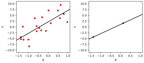
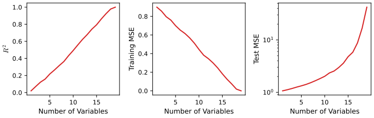
6.4.3 Regression in High Dimensions
Less flexible fitting methods (forward stepwise selection, ridge, the lasso, PCR) are exactly what is needed when \(p\) is large. Figure 6.24 shows the lasso with \(n=100\) and 20 truly associated features among \(p=20\), 50 or 2,000. For the lasso the degrees of freedom are the number of nonzero coefficients (plus one for the intercept).
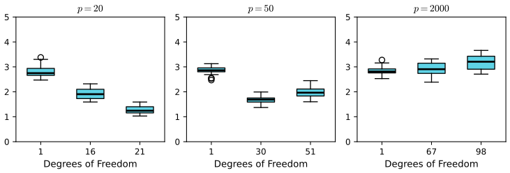
Three lessons: (1) regularisation is essential when \(p\) is large, (2) the tuning parameter must be chosen well, and (3) test error grows with the number of features unless the new features are truly associated with the response. The third point is the curse of dimensionality: noise features add variance (some get nonzero coefficients by chance) without reducing bias, and even relevant features cost variance that can outweigh their contribution.
6.4.4 Interpreting Results in High Dimensions
When \(p\gt n\) every predictor is an exact linear combination of the others (extreme collinearity), so we can never know which variables are truly predictive: a selected set of 17 SNPs is one of many sets that predict about as well, and another sample would likely select a different, perhaps disjoint, set. Report the model as one of many possible models, to be validated on independent data. And never report training RSS, \(p\)-values, \(R^2\) or other training-data measures of fit as evidence: with \(p\gt n\), \(R^2=1\) is guaranteed (Result 6.15). Report the error or \(R^2\) on an independent test set, or cross-validated.
6.5 Lab: Linear Models and Regularization Methods
The lab predicts a baseball player's Salary from 19 statistics of the previous season (Hitters data). Every step is shown in R (left; the R lab of James et al. 2021) and Python (right; the Python lab of James et al. 2023), written from scratch for this course: code/ch06_lab.R and code/ch06_lab.py. The Python version uses only pandas, numpy, statsmodels and scikit-learn; best subset selection, forward and backward selection are our own short functions. Both files run from start to finish; the outputs below are what they print.
Where R and Python agree, and where they differ
- Identical results wherever the computation is deterministic: the best subsets of every size, \(R^2\), the sizes chosen by \(C_p\), BIC and adjusted \(R^2\), all least squares coefficients, the forward and backward models, the ridge coefficients at a given \(\lambda\), and the variance explained by PCR and PLS.
- Different random splits. R uses
set.seed()exactly as the R edition, so the R column reproduces that edition's printed numbers (for example the test MSE 139,857 of cross-validated ridge). Python uses numpy's and scikit-learn's generators (for the training/test split, the Python edition's ownShuffleSplit(test_size=0.5, random_state=0)), so its validation and cross-validation numbers differ. They differ by about as much as two random splits in the same language would. - The scale of \(\lambda\). glmnet minimises \(\frac1{2n}\RSS+\lambda\big(\frac{1-\alpha}2\|\bb\|_2^2+\alpha\|\bb\|_1\big)\) on columns standardised with the \(1/n\) standard deviation, and for ridge it also divides \(y\) by its standard deviation \(s_y\) internally. So glmnet's ridge \(\lambda\) is scikit-learn's
Ridge(alpha=n*lambda/s_y)on standardised columns (and the Python edition'sElasticNet(alpha=lambda/s_y, l1_ratio=0)), while glmnet's lasso \(\lambda\) is exactly scikit-learn'sLasso(alpha=lambda). With this conversion the two languages print the same coefficients. Both differ from the \(\lambda\) of (6.5) and (6.7) used in the figures, which is \(2n\) times glmnet's lasso \(\lambda\).
Setup. Packages (R) and imports (Python). common.py holds the course's data loader and figure helper.
R
suppressPackageStartupMessages({
  library(ISLR2)    # the Hitters data
  library(leaps)    # regsubsets(): best subset, forward and backward selection
  library(glmnet)   # ridge regression and the lasso
  library(pls)      # pcr() and plsr()
})
.this_dir <- local({
  a <- grep("^--file=", commandArgs(FALSE), value = TRUE)
  if (length(a)) dirname(normalizePath(sub("^--file=", "", a[1]))) else getwd()
})
img_dir <- file.path(.this_dir, "..", "img", "ch06")
dir.create(img_dir, showWarnings = FALSE, recursive = TRUE)
step <- function(k, title) cat(sprintf("\n== [%s] %s\n", k, title))
options(width = 100, digits = 6)
Python
import os

for _v in ("OPENBLAS_NUM_THREADS", "MKL_NUM_THREADS", "OMP_NUM_THREADS"):
    os.environ.setdefault(_v, "1")

import itertools
import warnings

import numpy as np
import pandas as pd
import statsmodels.api as sm
import sklearn.linear_model as skl
import sklearn.model_selection as skm
from sklearn.cross_decomposition import PLSRegression
from sklearn.decomposition import PCA
from sklearn.pipeline import Pipeline
from sklearn.preprocessing import StandardScaler

from common import isl_data, savefig, plt, RED, BLUE, GREY

warnings.filterwarnings("ignore", category=UserWarning)
pd.set_option("display.width", 100)
np.set_printoptions(linewidth=100, suppress=True)


def step(k, title):
    print("\n== [%s] %s" % (k, title))
6.5.1 Subset Selection Methods
Step 1: the data. Salary is missing for 59 of the 322 players; we drop them. R's formula interface turns the three two-level factors into the dummies LeagueN, DivisionW, NewLeagueN; in Python we build the same 19 columns in the same order.
R
# -- [1] The Hitters data: drop the players whose salary is missing
step(1, "The data")
dim(Hitters)
sum(is.na(Hitters$Salary))
Hitters <- na.omit(Hitters)
dim(Hitters)
Python
# -- [1] The Hitters data: drop the players whose salary is missing
step(1, "The data")
Hitters = isl_data("Hitters")
print(Hitters.shape, Hitters["Salary"].isna().sum())
Hitters = Hitters.dropna()
print(Hitters.shape)
# The design matrix in the column order of R's model.matrix(): 0/1 dummies for the factors
num = ["AtBat", "Hits", "HmRun", "Runs", "RBI", "Walks", "Years", "CAtBat", "CHits", "CHmRun",
       "CRuns", "CRBI", "CWalks"]
X = Hitters[num].astype(float)
X["LeagueN"] = (Hitters["League"] == "N").astype(float)
X["DivisionW"] = (Hitters["Division"] == "W").astype(float)
for c in ["PutOuts", "Assists", "Errors"]:
    X[c] = Hitters[c].astype(float)
X["NewLeagueN"] = (Hitters["NewLeague"] == "N").astype(float)
y = Hitters["Salary"].to_numpy()
names = list(X.columns)
Xa = X.to_numpy()
n, p = Xa.shape
R output
[1] 322  20
[1] 59
[1] 263  20
Python output
(322, 20) 59
(263, 20)
Step 2: best subset selection. R's regsubsets() (package leaps) searches all subsets with a branch-and-bound algorithm; in Python we simply evaluate all \(2^{19}-1=524{,}287\) subsets, using \(\RSS=\by_c^\T\by_c-\bb_S^\T\bG_{SS}^{-1}\bb_S\) on the centred, scaled data and solving thousands of small systems at once (about 2 seconds). Same models, same \(R^2\) (from 32% with one variable to 55% with all), and the same choices: adjusted \(R^2\) picks 11 variables, \(C_p\) 10, BIC 6. (leaps reports Mallows' \(C'_p\) and the BIC \(n\log(\RSS/\TSS)+(d+1)\log n\); Python computes (6.2), (6.3) and leaps' BIC. The definitions rank models identically for \(C_p\), and here BIC's two versions also agree.)
R
# -- [2] Best subset selection: the best model of every size, and Cp, BIC, adjusted R^2
step(2, "Best subset selection")
regfit.full <- regsubsets(Salary ~ ., data = Hitters, nvmax = 19)
reg.summary <- summary(regfit.full)
round(reg.summary$rsq, 3)
c(adjr2 = which.max(reg.summary$adjr2), cp = which.min(reg.summary$cp),
  bic = which.min(reg.summary$bic))
coef(regfit.full, 6)

pdf(file.path(img_dir, "lab-r-criteria.pdf"), width = 8, height = 6)
par(mfrow = c(2, 2), mar = c(4.2, 4.2, 1, 1))
plot(reg.summary$rss, xlab = "Number of variables", ylab = "RSS", type = "l")
plot(reg.summary$adjr2, xlab = "Number of variables", ylab = "Adjusted RSq", type = "l")
points(11, reg.summary$adjr2[11], col = "red", cex = 2, pch = 20)
plot(reg.summary$cp, xlab = "Number of variables", ylab = "Cp", type = "l")
points(10, reg.summary$cp[10], col = "red", cex = 2, pch = 20)
plot(reg.summary$bic, xlab = "Number of variables", ylab = "BIC", type = "l")
points(6, reg.summary$bic[6], col = "red", cex = 2, pch = 20)
invisible(dev.off())
pdf(file.path(img_dir, "lab-r-bic-map.pdf"), width = 7, height = 5.5)
plot(regfit.full, scale = "bic")      # one row per model, black = variable included
invisible(dev.off())
Python
# -- [2] Best subset selection: the best model of every size, and Cp, BIC, adjusted R^2
step(2, "Best subset selection")
def best_subset(X, y, max_size=None):
    """For each size k, the subset of columns with the smallest RSS (with an intercept).
    Exhaustive: every subset's RSS is y'y - b'G^{-1}b on the centred, scaled data, solved in batches."""
    Z = (X - X.mean(0)) / X.std(0)
    yc = y - y.mean()
    G, b, tss = Z.T @ Z, Z.T @ yc, yc @ yc
    best = []
    for k in range(1, (max_size or X.shape[1]) + 1):
        combos = np.array(list(itertools.combinations(range(X.shape[1]), k)))
        rss = np.empty(len(combos))
        for a in range(0, len(combos), 20000):              # 92,378 subsets of size 9 or 10
            c = combos[a:a + 20000]
            sol = np.linalg.solve(G[c[:, :, None], c[:, None, :]], b[c][..., None])[..., 0]
            rss[a:a + 20000] = tss - (b[c] * sol).sum(1)
        i = np.argmin(rss)
        best.append((list(combos[i]), rss[i]))
    return best, tss


best, tss = best_subset(Xa, y)                               # 2^19 - 1 = 524,287 models
rss = np.array([r for _, r in best])
d = np.arange(1, p + 1)                                      # number of predictors
sigma2 = rss[-1] / (n - p - 1)                               # error variance from the full model
crit = pd.DataFrame({
    "rsq": 1 - rss / tss,
    "adjr2": 1 - (rss / (n - d - 1)) / (tss / (n - 1)),                  # (6.4)
    "Cp": (rss + 2 * d * sigma2) / n,                                      # (6.2)
    "BIC": (rss + np.log(n) * d * sigma2) / n,                             # (6.3)
    "BIC_leaps": n * np.log(rss / tss) + (d + 1) * np.log(n),             # R's summary()$bic
}, index=d)
print(crit["rsq"].round(3).to_numpy())
print({"adjr2": crit["adjr2"].idxmax(), "Cp": crit["Cp"].idxmin(), "BIC": crit["BIC"].idxmin(),
       "BIC_leaps": crit["BIC_leaps"].idxmin()})
cols6 = [names[j] for j in best[5][0]]
fit6 = sm.OLS(y, sm.add_constant(X[cols6])).fit()
print(fit6.params.round(6))

fig, axes = plt.subplots(2, 2, figsize=(8, 6))
for ax, col, lab, best_k in zip(axes.flat, ["rsq", "adjr2", "Cp", "BIC"],
                                ["$R^2$", "Adjusted $R^2$", "$C_p$", "BIC"],
                                [None, crit["adjr2"].idxmax(), crit["Cp"].idxmin(), crit["BIC"].idxmin()]):
    ax.plot(d, crit[col], color="k")
    if best_k is not None:
        ax.plot(best_k, crit[col][best_k], "o", color=RED, ms=8)
    ax.set_xlabel("Number of variables")
    ax.set_ylabel(lab)
fig.tight_layout()
savefig(fig, 6, "lab-py-criteria")
R output
 [1] 0.321 0.425 0.451 0.475 0.491 0.509 0.514 0.529 0.535 0.540 0.543 0.544 0.544 0.545 0.545 0.546
[17] 0.546 0.546 0.546
adjr2    cp   bic
   11    10     6
(Intercept)       AtBat        Hits       Walks        CRBI   DivisionW     PutOuts
  91.511798   -1.868589    7.604398    3.697647    0.643017 -122.951534    0.264308
Python output
[0.321 0.425 0.451 0.475 0.491 0.509 0.514 0.529 0.535 0.54  0.543 0.544 0.544 0.545 0.545 0.546
 0.546 0.546 0.546]
{'adjr2': 11, 'Cp': 10, 'BIC': 6, 'BIC_leaps': 6}
const         91.511798
AtBat         -1.868589
Hits           7.604398
Walks          3.697647
CRBI           0.643017
DivisionW   -122.951534
PutOuts        0.264308
dtype: float64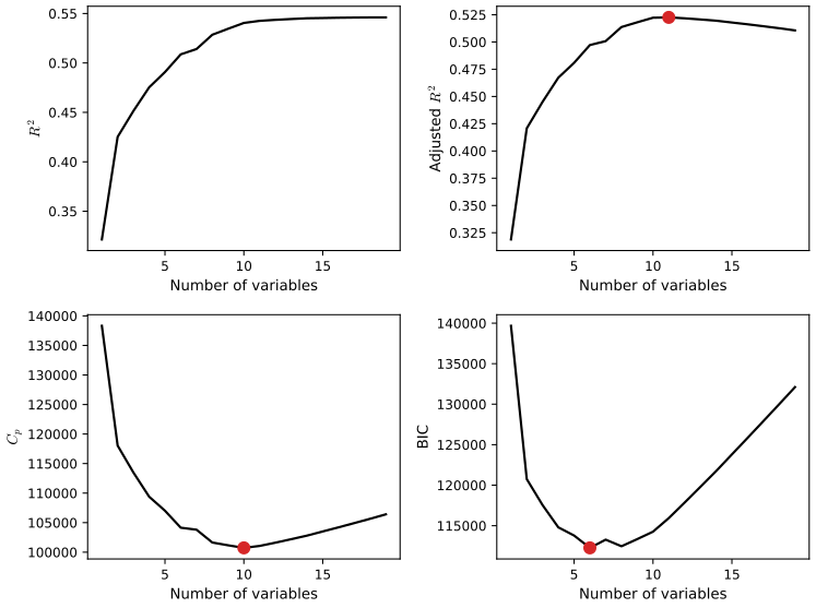
plot() and points(). Download: PDF · SVG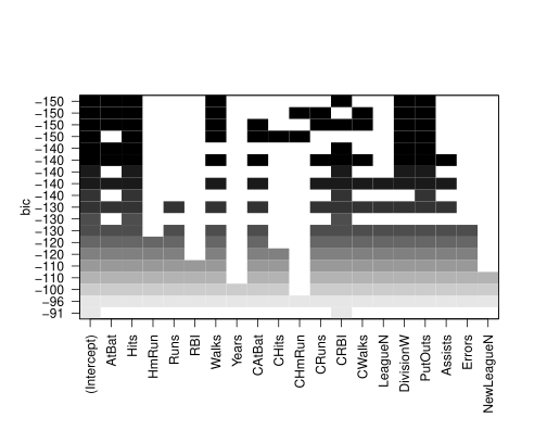
plot(regfit.full, scale = "bic"), the variables (black) in the best model of each size, ordered by BIC. The top row is the six-variable model AtBat, Hits, Walks, CRBI, DivisionW, PutOuts. This display is specific to leaps. Download: PDF · SVGStep 3: forward and backward stepwise selection. The best one- to six-variable models are the same for best subset and forward selection, but the three methods give three different seven-variable models. The Python edition chooses its forward-selection model by \(C_p\), stopping when \(C_p\) stops improving; the minimum of \(C_p\) along the forward path is the same 10-variable model in both languages.
R
# -- [3] Forward and backward stepwise selection
step(3, "Forward and backward stepwise selection")
regfit.fwd <- regsubsets(Salary ~ ., data = Hitters, nvmax = 19, method = "forward")
regfit.bwd <- regsubsets(Salary ~ ., data = Hitters, nvmax = 19, method = "backward")
round(coef(regfit.full, 7), 3)
round(coef(regfit.fwd, 7), 3)
round(coef(regfit.bwd, 7), 3)
# Cp along the forward path (the criterion the Python edition uses to stop forward selection)
fwd.summary <- summary(regfit.fwd)
which.min(fwd.summary$cp)
names(coef(regfit.fwd, which.min(fwd.summary$cp)))[-1]
Python
# -- [3] Forward and backward stepwise selection
step(3, "Forward and backward stepwise selection")
def rss_of(X, y, cols):
    A = np.column_stack([np.ones(len(y))] + [X[:, j] for j in cols])
    r = y - A @ np.linalg.lstsq(A, y, rcond=None)[0]
    return r @ r


def forward_stepwise(X, y):
    """Algorithm 6.2: add, one at a time, the variable that lowers the RSS most."""
    path, left = [[]], list(range(X.shape[1]))
    while left:
        j = min(left, key=lambda j: rss_of(X, y, path[-1] + [j]))
        path.append(path[-1] + [j])
        left.remove(j)
    return path                                              # path[k] = the k-variable model


def backward_stepwise(X, y):
    """Algorithm 6.3: drop, one at a time, the variable whose removal raises the RSS least."""
    path = [list(range(X.shape[1]))]
    while path[-1]:
        cur = path[-1]
        j = min(cur, key=lambda j: rss_of(X, y, [c for c in cur if c != j]))
        path.append([c for c in cur if c != j])
    return path[::-1]


fwd, bwd = forward_stepwise(Xa, y), backward_stepwise(Xa, y)
for label, cols in [("best", best[6][0]), ("forward", fwd[7]), ("backward", bwd[7])]:
    c = [names[j] for j in sorted(cols)]
    print(label, sm.OLS(y, sm.add_constant(X[c])).fit().params.round(3).to_dict())
# Cp along the forward path; the minimum is the model the Python edition's forward search stops at
cp_fwd = [(rss_of(Xa, y, fwd[k]) + 2 * k * sigma2) / n for k in range(p + 1)]
k_cp = int(np.argmin(cp_fwd))
print(k_cp, sorted(names[j] for j in fwd[k_cp]))
R output
(Intercept)        Hits       Walks      CAtBat       CHits      CHmRun   DivisionW     PutOuts
     79.451       1.283       3.227      -0.375       1.496       1.442    -129.987       0.237
(Intercept)       AtBat        Hits       Walks        CRBI      CWalks   DivisionW     PutOuts
    109.787      -1.959       7.450       4.913       0.854      -0.305    -127.122       0.253
(Intercept)       AtBat        Hits       Walks       CRuns      CWalks   DivisionW     PutOuts
    105.649      -1.976       6.757       6.056       1.129      -0.716    -116.169       0.303
[1] 10
 [1] "AtBat"     "Hits"      "Walks"     "CAtBat"    "CRuns"     "CRBI"      "CWalks"    "DivisionW"
 [9] "PutOuts"   "Assists"
Python output
best {'const': 79.451, 'Hits': 1.283, 'Walks': 3.227, 'CAtBat': -0.375, 'CHits': 1.496, 'CHmRun': 1.442, 'DivisionW': -129.987, 'PutOuts': 0.237}
forward {'const': 109.787, 'AtBat': -1.959, 'Hits': 7.45, 'Walks': 4.913, 'CRBI': 0.854, 'CWalks': -0.305, 'DivisionW': -127.122, 'PutOuts': 0.253}
backward {'const': 105.649, 'AtBat': -1.976, 'Hits': 6.757, 'Walks': 6.056, 'CRuns': 1.129, 'CWalks': -0.716, 'DivisionW': -116.169, 'PutOuts': 0.303}
10 ['Assists', 'AtBat', 'CAtBat', 'CRBI', 'CRuns', 'CWalks', 'DivisionW', 'Hits', 'PutOuts', 'Walks']
Step 4: choosing the size by a validation set and by cross-validation. The selection must be redone using only the training observations: inside the training half for the validation set, and inside each training fold for cross-validation. R's splits are the R edition's (validation chooses 7 variables, 10-fold CV chooses 10, as printed in the book); Python's splits are different and choose 4 and 8. The curves are flat beyond about 6 variables, so these choices are not stable across splits; the size chosen by cross-validation is then refitted on all 263 players.
R
# -- [4] Choosing the model size by a validation set and by 10-fold cross-validation
step(4, "Validation set and cross-validation")
set.seed(1)
train <- sample(c(TRUE, FALSE), nrow(Hitters), replace = TRUE)
test <- !train
regfit.best <- regsubsets(Salary ~ ., data = Hitters[train, ], nvmax = 19)
test.mat <- model.matrix(Salary ~ ., data = Hitters[test, ])
val.errors <- rep(NA, 19)
for (i in 1:19) {
  coefi <- coef(regfit.best, id = i)
  pred <- test.mat[, names(coefi)] %*% coefi
  val.errors[i] <- mean((Hitters$Salary[test] - pred)^2)
}
round(val.errors)
which.min(val.errors)

# regsubsets() has no predict() method, so we write one
predict.regsubsets <- function(object, newdata, id, ...) {
  form <- as.formula(object$call[[2]])
  mat <- model.matrix(form, newdata)
  coefi <- coef(object, id = id)
  mat[, names(coefi)] %*% coefi
}
k <- 10
n <- nrow(Hitters)
set.seed(1)
folds <- sample(rep(1:k, length = n))
cv.errors <- matrix(NA, k, 19, dimnames = list(NULL, paste(1:19)))
for (j in 1:k) {
  best.fit <- regsubsets(Salary ~ ., data = Hitters[folds != j, ], nvmax = 19)
  for (i in 1:19) {
    pred <- predict(best.fit, Hitters[folds == j, ], id = i)
    cv.errors[j, i] <- mean((Hitters$Salary[folds == j] - pred)^2)
  }
}
mean.cv.errors <- apply(cv.errors, 2, mean)
round(mean.cv.errors)
which.min(mean.cv.errors)
round(coef(regfit.full, 10), 3)   # the 10-variable model refitted on all the data
pdf(file.path(img_dir, "lab-r-cv-size.pdf"), width = 6, height = 4.5)
plot(mean.cv.errors, type = "b", xlab = "Number of variables", ylab = "10-fold CV error")
invisible(dev.off())
Python
# -- [4] Choosing the model size by a validation set and by 10-fold cross-validation
step(4, "Validation set and cross-validation")
def predict_subset(Xtr, ytr, Xte, cols):
    A = np.column_stack([np.ones(len(ytr))] + [Xtr[:, j] for j in cols])
    beta = np.linalg.lstsq(A, ytr, rcond=None)[0]
    return np.column_stack([np.ones(len(Xte))] + [Xte[:, j] for j in cols]) @ beta


rng = np.random.default_rng(1)
train = rng.choice([True, False], n)                         # about half the players
best_tr, _ = best_subset(Xa[train], y[train])                # selection on the training part only
val_errors = np.array([np.mean((y[~train] - predict_subset(Xa[train], y[train], Xa[~train], c)) ** 2)
                       for c, _ in best_tr])
print(val_errors.round(0))
print(int(np.argmin(val_errors)) + 1)

K = 10
folds = rng.permutation(np.arange(n) % K)
cv_errors = np.zeros((K, p))
for j in range(K):
    tr, te = folds != j, folds == j
    best_j, _ = best_subset(Xa[tr], y[tr])                   # best subset again inside every fold
    for i, (c, _) in enumerate(best_j):
        cv_errors[j, i] = np.mean((y[te] - predict_subset(Xa[tr], y[tr], Xa[te], c)) ** 2)
mean_cv = cv_errors.mean(0)
print(mean_cv.round(0))
k_cv = int(np.argmin(mean_cv)) + 1
print(k_cv, [names[j] for j in sorted(best[k_cv - 1][0])])

fig, ax = plt.subplots(figsize=(6, 4))
ax.plot(d, val_errors, "o--", color=BLUE, ms=4, label="validation set")
ax.plot(d, mean_cv, "o-", color=RED, ms=4, label="10-fold CV")
ax.set_xlabel("Number of variables")
ax.set_ylabel("Estimated test MSE")
ax.legend()
savefig(fig, 6, "lab-py-cv-size")
R output
 [1] 164377 144405 152176 145198 137902 139176 126849 136191 132890 135435 136963 140695 140691
[14] 141951 141508 142164 141767 142340 142238
[1] 7
     1      2      3      4      5      6      7      8      9     10     11     12     13     14
143440 126817 134214 131783 130766 120383 121443 114364 115163 109366 112738 113617 115558 115853
    15     16     17     18     19
115631 116050 116117 116419 116299
10
10
(Intercept)       AtBat        Hits       Walks      CAtBat       CRuns        CRBI      CWalks
    162.535      -2.169       6.918       5.773      -0.130       1.408       0.774      -0.831
  DivisionW     PutOuts     Assists
   -112.380       0.297       0.283
Python output
[215746. 183550. 185573. 159456. 173208. 170078. 170023. 169341. 164924. 174317. 169140. 164194.
 163615. 166164. 164143. 164331. 165353. 164706. 164492.]
4
[153371. 124385. 134876. 139742. 139400. 127575. 128102. 114736. 116183. 114964. 115624. 116998.
 119515. 121555. 121463. 121116. 121507. 121857. 121651.]
8 ['AtBat', 'Hits', 'Walks', 'CHmRun', 'CRuns', 'CWalks', 'DivisionW', 'PutOuts']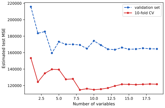
6.5.2 Ridge Regression and the Lasso
Step 5: ridge regression at fixed \(\lambda\). glmnet fits the whole path over a grid of 100 values from \(10^{10}\) to \(10^{-2}\). At \(\lambda=11{,}498\) the coefficients are tiny (\(\ell_2\) norm 6.36); at \(\lambda=705\) the norm is 57.1. Python's closed-form ridge on glmnet's scale gives the same numbers. At \(\lambda=50\), between grid points, we refit exactly: the R edition prints values interpolated along the grid (intercept 48.77), the exact answer is 47.72 in both languages. (glmnet needs a tight convergence threshold, thresh = 1e-12, to agree to three decimals.)
R
# -- [5] Ridge regression with glmnet: coefficients at fixed values of lambda
step(5, "Ridge regression at fixed lambda")
x <- model.matrix(Salary ~ ., Hitters)[, -1]   # 19 columns: the dummies LeagueN, DivisionW, NewLeagueN
y <- Hitters$Salary
grid <- 10^seq(10, -2, length = 100)
ridge.mod <- glmnet(x, y, alpha = 0, lambda = grid,   # alpha = 0: ridge; glmnet standardises x
                    control = list(thresh = 1e-12))  # tight convergence, so 3 decimals are exact
dim(coef(ridge.mod))
ridge.mod$lambda[50]
round(coef(ridge.mod)[, 50], 3)
sqrt(sum(coef(ridge.mod)[-1, 50]^2))
ridge.mod$lambda[60]
sqrt(sum(coef(ridge.mod)[-1, 60]^2))
# exact = TRUE refits at lambda = 50 instead of interpolating between grid values
round(predict(ridge.mod, s = 50, type = "coefficients", exact = TRUE, x = x, y = y)[1:20, ], 3)
Python
# -- [5] Ridge regression at fixed lambda, on glmnet's scale
step(5, "Ridge regression at fixed lambda")
def ridge_glmnet(X, y, lam):
    """Ridge with glmnet's conventions: columns standardised with the 1/n standard deviation, and
    glmnet's lambda equal to (2 sd(y)/n) times the lambda of (6.5) for the standardised columns.
    Returns (intercept, coefficients on the original scale)."""
    scaler = StandardScaler().fit(X)
    alpha = len(y) * lam / y.std()                           # sklearn's Ridge minimises RSS + alpha |b|^2
    fit = skl.Ridge(alpha=alpha).fit(scaler.transform(X), y)
    beta = fit.coef_ / scaler.scale_
    return y.mean() - scaler.mean_ @ beta, beta


grid = 10 ** np.linspace(10, -2, 100)                        # the R lab's grid, largest first
for lam in [grid[49], grid[59]]:
    b0, beta = ridge_glmnet(Xa, y, lam)
    print(round(lam, 2), round(b0, 3), round(np.sqrt(beta @ beta), 2))
b0, beta = ridge_glmnet(Xa, y, grid[49])
print(pd.Series(np.r_[b0, beta], ["(Intercept)"] + names).round(3).to_dict())
b0, beta = ridge_glmnet(Xa, y, 50)
print(pd.Series(np.r_[b0, beta], ["(Intercept)"] + names).round(3).to_dict())
R output
[1]  20 100
[1] 11497.6
(Intercept)       AtBat        Hits       HmRun        Runs         RBI       Walks       Years
    407.356       0.037       0.138       0.525       0.231       0.240       0.290       1.108
     CAtBat       CHits      CHmRun       CRuns        CRBI      CWalks     LeagueN   DivisionW
      0.003       0.012       0.088       0.023       0.024       0.025       0.085      -6.215
    PutOuts     Assists      Errors  NewLeagueN
      0.016       0.003      -0.021       0.301
[1] 6.36061
[1] 705.48
[1] 57.1096
(Intercept)       AtBat        Hits       HmRun        Runs         RBI       Walks       Years
     47.721      -0.353       1.954      -1.274       1.156       0.809       2.704      -6.121
     CAtBat       CHits      CHmRun       CRuns        CRBI      CWalks     LeagueN   DivisionW
      0.006       0.106       0.621       0.216       0.217      -0.147      45.845    -118.217
    PutOuts     Assists      Errors  NewLeagueN
      0.250       0.120      -3.277      -9.385
Python output
11497.57 407.356 6.36
705.48 54.354 57.11
{'(Intercept)': 407.356, 'AtBat': 0.037, 'Hits': 0.138, 'HmRun': 0.525, 'Runs': 0.231, 'RBI': 0.24, 'Walks': 0.29, 'Years': 1.108, 'CAtBat': 0.003, 'CHits': 0.012, 'CHmRun': 0.088, 'CRuns': 0.023, 'CRBI': 0.024, 'CWalks': 0.025, 'LeagueN': 0.085, 'DivisionW': -6.215, 'PutOuts': 0.016, 'Assists': 0.003, 'Errors': -0.021, 'NewLeagueN': 0.301}
{'(Intercept)': 47.723, 'AtBat': -0.353, 'Hits': 1.954, 'HmRun': -1.274, 'Runs': 1.156, 'RBI': 0.809, 'Walks': 2.705, 'Years': -6.121, 'CAtBat': 0.006, 'CHits': 0.106, 'CHmRun': 0.621, 'CRuns': 0.216, 'CRBI': 0.217, 'CWalks': -0.147, 'LeagueN': 45.845, 'DivisionW': -118.217, 'PutOuts': 0.25, 'Assists': 0.12, 'Errors': -3.277, 'NewLeagueN': -9.385}
Step 6: test error of ridge and the lasso, \(\lambda\) chosen by 10-fold cross-validation. In R (the R edition's split): \(\lambda=4\) gives test MSE 142,199, the intercept-only model 224,670 and least squares 168,589; cross-validation chooses \(\lambda=326\) (test MSE 139,857); the lasso chooses \(\lambda=9.29\) (test MSE 143,674) with 11 nonzero coefficients when refitted on all the data. Python's split gives smaller errors throughout (126,210; 231,853; 134,597; ridge 128,890 at \(\lambda=394\); lasso 129,878 at \(\lambda=8.0\) with 11 nonzero coefficients) and the same ranking: both penalised fits beat least squares and the null model and are close to each other. The last lines repeat the Python edition's own computation, 5-fold ElasticNetCV on all 263 players, and reproduce its printed numbers exactly: ridge \(\alpha=0.01185\) (glmnet's \(\lambda=0.01185\,s_y=5.3\)) with CV MSE 115,526.71, and the lasso \(\alpha=3.147\) with CV MSE 114,690.73 and 6 zero coefficients.
R
# -- [6] Ridge and the lasso on a training/test split, lambda chosen by 10-fold CV
step(6, "Ridge and the lasso: test error")
set.seed(1)
train <- sample(1:nrow(x), nrow(x) / 2)
test <- (-train)
y.test <- y[test]
ridge.mod <- glmnet(x[train, ], y[train], alpha = 0, lambda = grid,
                    control = list(thresh = 1e-12))
ridge.pred <- predict(ridge.mod, s = 4, newx = x[test, ])
mean((ridge.pred - y.test)^2)                       # lambda = 4
mean((mean(y[train]) - y.test)^2)                   # intercept only
ridge.pred <- predict(ridge.mod, s = 0, newx = x[test, ], exact = TRUE, x = x[train, ], y = y[train])
mean((ridge.pred - y.test)^2)                       # lambda = 0: least squares
set.seed(1)
cv.out <- cv.glmnet(x[train, ], y[train], alpha = 0)
bestlam <- cv.out$lambda.min
bestlam
ridge.pred <- predict(ridge.mod, s = bestlam, newx = x[test, ])
mean((ridge.pred - y.test)^2)
out <- glmnet(x, y, alpha = 0)
round(predict(out, type = "coefficients", s = bestlam)[1:20, ], 2)
pdf(file.path(img_dir, "lab-r-cv-ridge.pdf"), width = 6, height = 4.5)
plot(cv.out)
invisible(dev.off())

lasso.mod <- glmnet(x[train, ], y[train], alpha = 1, lambda = grid)
set.seed(1)
cv.out <- cv.glmnet(x[train, ], y[train], alpha = 1)
bestlam <- cv.out$lambda.min
bestlam
lasso.pred <- predict(lasso.mod, s = bestlam, newx = x[test, ])
mean((lasso.pred - y.test)^2)
out <- glmnet(x, y, alpha = 1, lambda = grid)
lasso.coef <- predict(out, type = "coefficients", s = bestlam)[1:20, ]
round(lasso.coef[lasso.coef != 0], 2)
sum(lasso.coef[-1] != 0)
pdf(file.path(img_dir, "lab-r-lasso-path.pdf"), width = 6, height = 4.5)
plot(lasso.mod, xvar = "lambda")
invisible(dev.off())
Python
# -- [6] Ridge and the lasso on a training/test split, lambda chosen by 10-fold CV
step(6, "Ridge and the lasso: test error")
split = skm.ShuffleSplit(n_splits=1, test_size=0.5, random_state=0)   # the Python edition's split
tr, te = next(split.split(Xa))
def test_mse(pred):
    return np.mean((pred - y[te]) ** 2)


b0, beta = ridge_glmnet(Xa[tr], y[tr], 4)
print(round(test_mse(b0 + Xa[te] @ beta)))                   # lambda = 4
print(round(test_mse(np.full(len(te), y[tr].mean()))))       # intercept only
ls_fit = skl.LinearRegression().fit(Xa[tr], y[tr])
print(round(test_mse(ls_fit.predict(Xa[te]))))               # least squares
kfold = skm.KFold(10, shuffle=True, random_state=0)
lam_grid = 10 ** np.linspace(5, -2, 100)


def cv_lambda(fit_predict, X, y, lams, cv):
    """Mean CV error for each lambda; standardisation is redone inside every fold, as glmnet does."""
    err = np.zeros((cv.get_n_splits(), len(lams)))
    for f, (a, b) in enumerate(cv.split(X)):
        for i, lam in enumerate(lams):
            err[f, i] = np.mean((y[b] - fit_predict(X[a], y[a], X[b], lam)) ** 2)
    return err.mean(0), err.std(0) / np.sqrt(err.shape[0])


def ridge_fp(Xtr, ytr, Xte, lam):
    b0, beta = ridge_glmnet(Xtr, ytr, lam)
    return b0 + Xte @ beta


def lasso_glmnet(X, y, lam):
    """The lasso on glmnet's scale: sklearn's Lasso minimises RSS/(2n) + alpha |b|_1, which is
    glmnet's criterion when alpha = lambda and the columns are standardised (1/n sd)."""
    scaler = StandardScaler().fit(X)
    fit = skl.Lasso(alpha=lam, tol=1e-10, max_iter=100000).fit(scaler.transform(X), y)
    beta = fit.coef_ / scaler.scale_
    return y.mean() - scaler.mean_ @ beta, beta


def lasso_fp(Xtr, ytr, Xte, lam):
    b0, beta = lasso_glmnet(Xtr, ytr, lam)
    return b0 + Xte @ beta


cv_r, se_r = cv_lambda(ridge_fp, Xa[tr], y[tr], lam_grid, kfold)
lam_r = lam_grid[np.argmin(cv_r)]
b0, beta = ridge_glmnet(Xa[tr], y[tr], lam_r)
print(round(lam_r, 2), round(test_mse(b0 + Xa[te] @ beta)))
b0, beta = ridge_glmnet(Xa, y, lam_r)                        # refit on all the data
print(pd.Series(np.r_[b0, beta], ["(Intercept)"] + names).round(2).to_dict())

lam_grid_l = 10 ** np.linspace(2.5, -2, 80)
cv_l, se_l = cv_lambda(lasso_fp, Xa[tr], y[tr], lam_grid_l, kfold)
lam_l = lam_grid_l[np.argmin(cv_l)]
b0, beta = lasso_glmnet(Xa[tr], y[tr], lam_l)
print(round(lam_l, 2), round(test_mse(b0 + Xa[te] @ beta)))
b0, beta = lasso_glmnet(Xa, y, lam_l)
coef_l = pd.Series(np.r_[b0, beta], ["(Intercept)"] + names)
print(coef_l[coef_l != 0].round(2).to_dict())
print(int((beta != 0).sum()))

fig, axes = plt.subplots(1, 2, figsize=(9, 3.8))
for ax, lams, cv, se, best_lam, title in [(axes[0], lam_grid, cv_r, se_r, lam_r, "Ridge"),
                                          (axes[1], lam_grid_l, cv_l, se_l, lam_l, "Lasso")]:
    ax.errorbar(np.log(lams), cv, yerr=se, color=RED, ecolor="#cccccc", lw=1.4)
    ax.axvline(np.log(best_lam), color="k", ls="--", lw=1)
    ax.set_xlabel(r"$\log(\lambda)$ (glmnet scale)")
    ax.set_ylabel("10-fold CV MSE")
    ax.set_title(title)
fig.tight_layout()
savefig(fig, 6, "lab-py-cv-lambda")

# The same questions as the Python edition asks them: 5-fold CV on all 263 players, with
# scikit-learn's ElasticNetCV (its alpha is glmnet's lambda divided by sd(y) for ridge)
kfold5 = skm.KFold(5, shuffle=True, random_state=0)
alphas = 10 ** np.linspace(8, -2, 100) / y.std()
ridgeCV = Pipeline([("scaler", StandardScaler()),
                    ("ridge", skl.ElasticNetCV(alphas=alphas, l1_ratio=0, cv=kfold5))]).fit(Xa, y)
tuned = ridgeCV.named_steps["ridge"]
print(round(tuned.alpha_, 5), round(tuned.mse_path_.mean(1).min(), 2))
lassoCV = Pipeline([("scaler", StandardScaler()),
                    ("lasso", skl.ElasticNetCV(n_alphas=100, l1_ratio=1, cv=kfold5))]).fit(Xa, y)
tuned = lassoCV.named_steps["lasso"]
print(round(tuned.alpha_, 3), round(tuned.mse_path_.mean(1).min(), 2), int((tuned.coef_ == 0).sum()))

lasso_path = np.array([lasso_glmnet(Xa[tr], y[tr], lam)[1] * Xa[tr].std(0) for lam in lam_grid_l])
fig, ax = plt.subplots(figsize=(6, 4))
ax.plot(np.log(lam_grid_l), lasso_path, lw=1.2)
ax.axhline(0, color=GREY, lw=0.6)
ax.set_xlabel(r"$\log(\lambda)$ (glmnet scale)")
ax.set_ylabel("Standardised coefficients")
savefig(fig, 6, "lab-py-lasso-path")
R output
[1] 142199
[1] 224670
[1] 168589
[1] 326.083
[1] 139857
(Intercept)       AtBat        Hits       HmRun        Runs         RBI       Walks       Years
      15.44        0.08        0.86        0.60        1.06        0.88        1.62        1.35
     CAtBat       CHits      CHmRun       CRuns        CRBI      CWalks     LeagueN   DivisionW
       0.01        0.06        0.41        0.11        0.12        0.05       22.09      -79.04
    PutOuts     Assists      Errors  NewLeagueN
       0.17        0.03       -1.36        9.12
[1] 9.28695
[1] 143674
(Intercept)       AtBat        Hits       Walks       Years      CHmRun       CRuns        CRBI
       1.27       -0.05        2.18        2.29       -0.34        0.03        0.22        0.42
    LeagueN   DivisionW     PutOuts      Errors
      20.29     -116.17        0.24       -0.86
[1] 11
Python output
126210
231853
134597
394.42 128890
{'(Intercept)': 21.16, 'AtBat': 0.09, 'Hits': 0.8, 'HmRun': 0.78, 'Runs': 1.04, 'RBI': 0.88, 'Walks': 1.55, 'Years': 1.79, 'CAtBat': 0.01, 'CHits': 0.05, 'CHmRun': 0.39, 'CRuns': 0.11, 'CRBI': 0.11, 'CWalks': 0.06, 'LeagueN': 19.93, 'DivisionW': -73.06, 'PutOuts': 0.15, 'Assists': 0.03, 'Errors': -1.18, 'NewLeagueN': 9.44}
8.04 129878
{'(Intercept)': 2.95, 'AtBat': -0.13, 'Hits': 2.43, 'Walks': 2.32, 'Years': -0.64, 'CHmRun': 0.07, 'CRuns': 0.23, 'CRBI': 0.4, 'LeagueN': 23.57, 'DivisionW': -117.63, 'PutOuts': 0.24, 'Errors': -0.99}
11
0.01185 115526.71
3.147 114690.73 6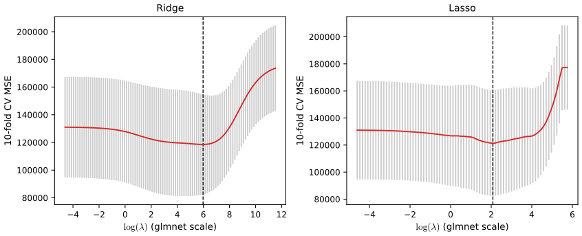
plot(cv.out) shows the same kind of curve. Download: PDF · SVG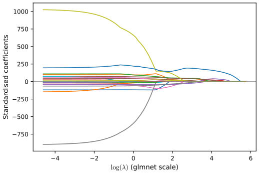
plot(lasso.mod, xvar = "lambda"). Download: PDF · SVG6.5.3 PCR and PLS Regression
Step 7: principal components regression. The variance explained is deterministic and identical: 38.31% of the variance of the predictors with one component, 84.29% with five; 40.63% of the variance of Salary with one component and 44.90% with five. Cross-validation on all the data puts the minimum at 18 components in R and 16 in Python, but the curve is nearly flat from \(M=1\). On the training half R's cross-validation chooses \(M=5\) (test MSE 142,812, as in the R edition) and Python's \(M=1\) (137,658; with \(M=5\) it would be 130,105). Two notes: scikit-learn's PCA may flip the sign of a component (the Python edition prints \(-21.60\) where we get \(+21.60\)); signs of principal components are arbitrary and the fit is unchanged.
R
# -- [7] Principal components regression
step(7, "Principal components regression")
set.seed(2)
pcr.fit <- pcr(Salary ~ ., data = Hitters, scale = TRUE, validation = "CV")
round(explvar(pcr.fit)[1:5], 2)                     # % variance of X per component
round(cumsum(explvar(pcr.fit))[1:5], 2)             # cumulative % of X
round(drop(R2(pcr.fit, estimate = "train", intercept = FALSE)$val)[1:5] * 100, 2)  # % of Salary
cv.rmsep <- drop(RMSEP(pcr.fit, estimate = "CV")$val)  # entries for 0, 1, ..., 19 components
round(cv.rmsep[1:5], 1)
which.min(cv.rmsep) - 1                             # number of components with the lowest CV error
set.seed(1)
pcr.fit <- pcr(Salary ~ ., data = Hitters, subset = train, scale = TRUE, validation = "CV")
which.min(drop(RMSEP(pcr.fit, estimate = "CV")$val)) - 1
pcr.pred <- predict(pcr.fit, x[test, ], ncomp = 5)
mean((pcr.pred - y.test)^2)
pdf(file.path(img_dir, "lab-r-pcr.pdf"), width = 6, height = 4.5)
validationplot(pcr.fit, val.type = "MSEP")
invisible(dev.off())
Python
# -- [7] Principal components regression
step(7, "Principal components regression")
def pcr(M):
    return Pipeline([("scaler", StandardScaler()), ("pca", PCA(n_components=M)),
                     ("ols", skl.LinearRegression())])


pca = PCA().fit(StandardScaler().fit_transform(Xa))
print((100 * pca.explained_variance_ratio_[:5]).round(2))
print((100 * np.cumsum(pca.explained_variance_ratio_)[:5]).round(2))
print(np.array([100 * pcr(M).fit(Xa, y).score(Xa, y) for M in range(1, 6)]).round(2))   # % of Salary


def cv_components(make, X, y, cv, Ms):
    """CV MSE for M = 0 (intercept only) and each M in Ms."""
    err = np.zeros((cv.get_n_splits(), len(Ms) + 1))
    for f, (a, b) in enumerate(cv.split(X)):
        err[f, 0] = np.mean((y[b] - y[a].mean()) ** 2)
        for i, M in enumerate(Ms, 1):
            err[f, i] = np.mean((y[b] - make(M).fit(X[a], y[a]).predict(X[b]).ravel()) ** 2)
    return err.mean(0)


Ms = range(1, p + 1)
cv_pcr_all = cv_components(pcr, Xa, y, kfold, Ms)
print(np.sqrt(cv_pcr_all[:5]).round(1), int(np.argmin(cv_pcr_all)))     # RMSE, like R's summary
cv_pcr = cv_components(pcr, Xa[tr], y[tr], kfold, Ms)
M_pcr = int(np.argmin(cv_pcr))
print(M_pcr, round(test_mse(pcr(M_pcr).fit(Xa[tr], y[tr]).predict(Xa[te]))),
      round(test_mse(pcr(5).fit(Xa[tr], y[tr]).predict(Xa[te]))))
R output
Comp 1 Comp 2 Comp 3 Comp 4 Comp 5
 38.31  21.84  10.69   8.19   5.26
Comp 1 Comp 2 Comp 3 Comp 4 Comp 5
 38.31  60.16  70.84  79.03  84.29
1 comps 2 comps 3 comps 4 comps 5 comps
  40.63   41.58   42.17   43.22   44.90
(Intercept)     1 comps     2 comps     3 comps     4 comps
      452.0       351.9       353.2       355.0       352.8
18 comps
      18
5 comps
      5
[1] 142812
Python output
[38.31 21.84 10.69  8.19  5.26]
[38.31 60.16 70.84 79.03 84.29]
[40.63 41.58 42.17 43.22 44.9 ]
[450.9 348.4 347.6 347.5 345. ] 16
1 137658 130105
Step 8: partial least squares. Both languages choose a single PLS direction on the training half (R: test MSE 151,995; Python: 133,248). On all the data, one PLS direction explains 38.08% of the variance of the predictors and 43.05% of that of Salary, in both languages: almost as much of Salary as five principal components (44.90%), because PLS looks for directions that explain the response. (scikit-learn's PLSRegression scales with the \(n-1\) standard deviation; the variance fraction must be computed on the same scaling to get 38.08.)
R
# -- [8] Partial least squares
step(8, "Partial least squares")
set.seed(1)
pls.fit <- plsr(Salary ~ ., data = Hitters, subset = train, scale = TRUE, validation = "CV")
round(drop(RMSEP(pls.fit, estimate = "CV")$val)[1:5], 1)
which.min(drop(RMSEP(pls.fit, estimate = "CV")$val)) - 1
pls.pred <- predict(pls.fit, x[test, ], ncomp = 1)
mean((pls.pred - y.test)^2)
pls.fit <- plsr(Salary ~ ., data = Hitters, scale = TRUE, ncomp = 1)
round(c(X = explvar(pls.fit)[1],
        Salary = 100 * drop(R2(pls.fit, estimate = "train", intercept = FALSE)$val)), 2)
Python
# -- [8] Partial least squares
step(8, "Partial least squares")
def pls(M):
    return PLSRegression(n_components=M, scale=True)


cv_pls = cv_components(pls, Xa[tr], y[tr], kfold, Ms)
M_pls = int(np.argmin(cv_pls))
print(np.sqrt(cv_pls[:5]).round(1), M_pls)
print(round(test_mse(pls(M_pls).fit(Xa[tr], y[tr]).predict(Xa[te]).ravel())),
      round(test_mse(pls(1).fit(Xa[tr], y[tr]).predict(Xa[te]).ravel())))
pls1 = pls(1).fit(Xa, y)
Z = (Xa - Xa.mean(0)) / Xa.std(0, ddof=1)                  # PLSRegression scales with ddof = 1
T, P = pls1.x_scores_, pls1.x_loadings_
x_expl = 100 * np.sum((T @ P.T) ** 2) / np.sum(Z ** 2)       # % of the variance of X captured
print(round(x_expl, 2), round(100 * pls1.score(Xa, y), 2))

fig, axes = plt.subplots(1, 2, figsize=(9, 3.8), sharey=True)
for ax, cv, Mbest, title in [(axes[0], cv_pcr, M_pcr, "PCR"), (axes[1], cv_pls, M_pls, "PLS")]:
    ax.plot(range(0, p + 1), cv, "o-", color=RED, ms=4)
    ax.axvline(Mbest, color="k", ls="--", lw=1)
    ax.set_xlabel("Number of components M")
    ax.set_title(title)
axes[0].set_ylabel("10-fold CV MSE (training half)")
fig.tight_layout()
savefig(fig, 6, "lab-py-pcr-pls")
R output
(Intercept)     1 comps     2 comps     3 comps     4 comps
      428.3       325.5       329.9       328.8       339.0
1 comps
      1
[1] 151995
X.Comp 1   Salary
   38.08    43.05
Python output
[421.  343.1 351.1 347.6 360.5] 1
133248 133248
38.08 43.05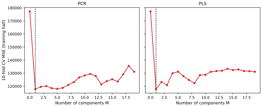
Notes on the book
Points where the text, a figure or a lab disagrees with an exact computation, with the evidence. None changes the chapter's message.
1. Section 6.4.1: present and absent are swapped both editions
In the bag-of-words example "each of the \(p\) search terms is scored present (0) or absent (1)". The usual coding, and the one implied by "binary feature vector" of indicators, is present = 1 and absent = 0.
2. Figure 6.12: the vertical axis is the cross-validation MSE divided by \(n\) both editions
The left panel's "Cross-Validation Error" runs from 25.0 to 25.6. A mean squared error for Balance (standard deviation 460) cannot be that small: the residual variance of the full model alone is \(\hat\sigma^2=9{,}760\). Our exact leave-one-out errors for ridge on the Credit data run from 10,065 (minimum, at \(\lambda=0.35\)) to 10,217 at \(\lambda=5\); divided by \(n=400\) they are 25.16 and 25.54, which matches the book's axis and the shape of its curve, including the position of the dashed line (Figure 6.12 above). So the plotted quantity is \(\mathrm{CV}_{(n)}/n\) (or the sum of squared leave-one-out errors divided by \(n^2\)), not the MSE.
3. Section 6.3.1: loadings 0.839 and 0.544 cannot come from standardised variables (6.19)–(6.20) and footnote 6
Footnote 6 says the principal components were computed after standardising pop and ad. For any two standardised variables with nonzero correlation the first principal component direction is \((1,1)/\sqrt2\) or \((1,-1)/\sqrt2\), loadings \(\pm0.707\) (Filling the gap 6.12). The printed loadings 0.839 and 0.544 therefore belong to the unstandardised data, and so do the scores \(-26.1\) and \(18.7\) quoted from (6.20) and the horizontal scale of Figure 6.15 (about \(\pm20\)). Figure 6.16's scale (about \(\pm3\)) is that of standardised scores. Our simulated cities show both: unstandardised loadings \((0.839,0.544)\), scores from \(-23.8\) to \(18.4\); standardised loadings \((0.707,0.707)\), scores within \(\pm2.3\).
4. Figure 6.24: 111 degrees of freedom with \(n=100\) both editions
The caption defines the lasso's degrees of freedom as the number of nonzero coefficients and says \(n=100\). With the response and predictors centred for the intercept, a lasso solution (the one computed by the usual algorithms, unique when the predictors are in general position) has at most \(n-1=99\) nonzero coefficients (Tibshirani 2013), so the degrees of freedom, counting the intercept, are at most 100. The label 111 for \(p=2000\) is impossible under the stated setup; in our reproduction the least regularised fit has 98 on average. The book's conclusion (the lasso fails for \(p=2000\) at every \(\lambda\)) is unaffected.
5. Python edition, ridge on a validation set: the scaler is left out James et al. (2023), Section 6.5.2, In[30]–[31]
The text sets up the pipeline pipe (scaler, then ridge) and says the pipeline can be passed to cross_validate(), but the code passes ridge alone, so the fit uses the unstandardised predictors. Evidence: with the edition's split and \(\alpha=0.01\), ridge on the raw predictors gives exactly the printed 134,214.00, and the pipeline with standardisation gives 126,241.37. The intercept-only result (231,788.32) is unaffected.
6. Python edition: cross-validation errors called test errors, and a \(\lambda=4\) that never appears James et al. (2023), Section 6.5.2, after In[39] and In[46]
"What is the test MSE associated with this value of \(\lambda\)?" is answered with np.min(tuned_ridge.mse_path_.mean(1)) = 115,526.71, which is the minimum cross-validation error over the grid on all 263 players (a slightly optimistic estimate, not a test error); the lasso's 114,690.73 is described the same way. The next sentence, "a further improvement over the test MSE that we got using \(\lambda=4\)", is carried over from the R edition: the Python lab never fits \(\lambda=4\). The nested estimate the edition computes next (132,393.84) is the honest test-error estimate.
7. Python edition: 0.0114 printed as 0.114 James et al. (2023), Section 6.5.1, after In[21]
The output shows 'lambda_0': 0.011416...; the text says the penalty parameter is "0.114".
8. Smaller points
- Footnote 3: "Mallow's \(C_p\)" should be "Mallows' \(C_p\)" (after Colin Mallows).
- Section 6.2.3 and Figure 6.13: the claim that least squares gives a large coefficient to only one of the two signal variables depends on the sample; in our simulated data set both are large (12.1 and 9.6). At the minimum of our CV curve the lasso keeps the two signal variables and five noise variables with coefficients below 0.41 in absolute value; the one-standard-error rule keeps exactly the two signal variables.
- R edition, Section 6.5.2:
predict(ridge.mod, s = 50, type = "coefficients")withoutexact = TRUEinterpolates between grid values, so the printed coefficients (intercept 48.766) are approximate; the exact ridge fit at \(\lambda=50\) has intercept 47.723 (lab step 5). - Python edition, In[57]: the PLS plot is labelled "# principal components"; the components are PLS directions.
6.6 Exercises
All eleven exercises, restated in my own words, with complete solutions (hidden). The applied solutions are the last sections of ch06_lab.R and ch06_lab.py; the two languages use different random numbers, so their numbers differ while their conclusions agree.
Conceptual
Exercise 6.1. Best subset, forward and backward stepwise selection are run on the same data, each giving models with \(0,1,\dots,p\) predictors. (a) Which of the three \(k\)-predictor models has the smallest training RSS? (b) Which has the smallest test RSS? (c) True or false: (i) forward's \(k\)-model is contained in forward's \((k+1)\)-model; (ii) the same for backward; (iii) backward's \(k\)-model is contained in forward's \((k+1)\)-model; (iv) forward's \(k\)-model is contained in backward's \((k+1)\)-model; (v) best subset's \(k\)-model is contained in best subset's \((k+1)\)-model.
Solution
(a) Best subset: it minimises the training RSS over all \(k\)-subsets, which include the two stepwise models (ties are possible, e.g. for \(k=0,1\) and \(k=p\) with forward and backward respectively). (b) No general answer: test RSS is not what any of the methods optimises. Best subset searches a larger space and may overfit; a stepwise model can have the smaller test error, and often the three are close. (c) (i) True: forward adds one variable at a time. (ii) True: backward removes one at a time, so going up from \(k\) to \(k+1\) adds one back. (iii) False in general. (iv) False in general. On the Credit data (Table 6.1) backward's one-variable model {Limit} is not in forward's two-variable model {Rating, Income}, and forward's {Rating} is not in backward's {Limit, Income}. (v) False: the best four-variable Credit model {Income, Limit, Cards, Student} does not contain the best three {Income, Rating, Student}.
Exercise 6.2. Relative to least squares, is (a) the lasso, (b) ridge regression, (c) a non-linear method: i. more flexible, better when its increase in bias is less than its decrease in variance; ii. more flexible, better when its increase in variance is less than its decrease in bias; iii. less flexible, better when its increase in bias is less than its decrease in variance; iv. less flexible, better when its increase in variance is less than its decrease in bias?
Solution
(a) iii: the lasso restricts the coefficients (a budget \(s\) smaller than the least squares norm), adding bias and removing variance; it helps when the variance saved exceeds the bias added. (b) iii, for the same reason (Result 6.7). (c) ii: non-linear methods are more flexible than a linear fit; they add variance and help when they remove more (squared) bias than that, i.e. when the true relationship is far from linear.
Exercise 6.3. Estimate the coefficients by minimising the RSS subject to \(\sum_j|\beta_j|\le s\). As \(s\) increases from 0, what happens to (a) training RSS, (b) test RSS, (c) variance, (d) squared bias, (e) irreducible error? Choose from: i. increase then decrease (inverted U); ii. decrease then increase (U); iii. steadily increase; iv. steadily decrease; v. remain constant.
Solution
\(s=0\) is the null model; large \(s\) is least squares. (a) iv: the feasible set grows, so the minimum RSS can only fall, until it reaches the least squares RSS (then constant). (b) ii: first falls as genuine signal is fitted, then rises as the fit starts fitting noise (the U of Figures 6.8 and 6.9, read from right to left). (c) iii: more flexibility, more variance. (d) iv: less constraint, less bias. (e) v: \(\Var(\epsilon)\) does not depend on the model.
Exercise 6.4. The same questions for ridge regression, (6.5), as \(\lambda\) increases from 0.
Solution
Increasing \(\lambda\) moves from least squares to the null model, the reverse of Exercise 6.3. (a) iii: training RSS increases steadily (from the least squares minimum). (b) ii: test RSS typically decreases first (variance falls faster than bias rises) and then increases (Figure 6.5). (c) iv: variance decreases steadily. (d) iii: squared bias increases steadily. (e) v: constant.
Exercise 6.5. Let \(n=p=2\), \(x_{11}=x_{12}\), \(x_{21}=x_{22}\), and \(y_1+y_2=0\), \(x_{11}+x_{21}=0\), \(x_{12}+x_{22}=0\), so the intercept estimate is 0. (a) Write the ridge problem. (b) Show that the ridge estimates satisfy \(\hat\beta_1=\hat\beta_2\). (c) Write the lasso problem. (d) Show that the lasso solution is not unique, and describe all solutions.
Solution
Write \(a=x_{11}=x_{12}\), so \(x_{21}=x_{22}=-a\), and \(y_2=-y_1\). Each fitted value depends on the coefficients only through \(t=\beta_1+\beta_2\): \(\hat y_1=at\), \(\hat y_2=-at\). So \(\RSS=(y_1-at)^2+(-y_1+at)^2=2(y_1-at)^2\).
(a) Minimise \(2(y_1-a(\beta_1+\beta_2))^2+\lambda(\beta_1^2+\beta_2^2)\). (b) For a fixed sum \(t\), \(\beta_1^2+\beta_2^2=\frac{t^2}2+\frac{(\beta_1-\beta_2)^2}2\) is smallest when \(\beta_1=\beta_2=t/2\); the RSS does not care how \(t\) is split, so the minimiser has \(\hat\beta_1=\hat\beta_2\). Minimising \(2(y_1-at)^2+\lambda t^2/2\) over \(t\) gives \(t=4ay_1/(4a^2+\lambda)\), so \(\hat\beta_1=\hat\beta_2=2ay_1/(4a^2+\lambda)\): the two copies share the effect equally.
(c) Minimise \(2(y_1-a(\beta_1+\beta_2))^2+\lambda(|\beta_1|+|\beta_2|)\). (d) \(|\beta_1|+|\beta_2|\ge|\beta_1+\beta_2|=|t|\), with equality whenever \(\beta_1\) and \(\beta_2\) have the same sign (or one is 0). So the problem reduces to minimising \(2(y_1-at)^2+\lambda|t|\) over \(t\), a one-dimensional lasso with solution \(\hat t=\sign(y_1/a)\big(|y_1/a|-\lambda/(4a^2)\big)_+\) (as in Filling the gap 6.9). Every pair with \(\beta_1+\beta_2=\hat t\) and \(\beta_1\beta_2\ge0\) attains the minimum: the whole segment from \((\hat t,0)\) to \((0,\hat t)\), the edge of the diamond \(|\beta_1|+|\beta_2|\le|\hat t|\). Geometrically the RSS contours here are lines parallel to that edge, so they touch the diamond along a side rather than at a corner.
Exercise 6.6. (a) With \(p=1\), choose \(y_1\) and \(\lambda\gt0\) and plot (6.12) as a function of \(\beta_1\); confirm that it is minimised by (6.14). (b) Do the same for (6.13) and (6.15).
Solution
Take \(y_1=2\), \(\lambda=2\). (a) \((2-\beta)^2+2\beta^2=3\beta^2-4\beta+4\), a parabola with vertex at \(\beta=2/3=y_1/(1+\lambda)\), as (6.14) says; its minimum value is \(8/3\). (b) \((2-\beta)^2+2|\beta|\): for \(\beta\gt0\) this is \(\beta^2-2\beta+4\), minimised at \(\beta=1=y_1-\lambda/2\), value 3; for \(\beta\lt0\) it is \(\beta^2-6\beta+4\), decreasing up to 0 (value 4 at \(\beta=0\)). So the minimum is at \(\beta=1\), as (6.15) says. With \(y_1=0.5\), \(\lambda=2\) instead, the kink at 0 is the minimum (\(|y_1|\le\lambda/2\)): soft thresholding sets the estimate to 0. The demonstration plots both criteria for any \(y_1\) and \(\lambda\):
▶ DemoThe one-dimensional ridge and lasso criteriaDrag y and λ; the minimiser of each curve follows (6.14) and (6.15).Exercise 6.7. Let \(y_i=\beta_0+\sum_jx_{ij}\beta_j+\epsilon_i\) with \(\epsilon_i\) i.i.d. \(\N(0,\sigma^2)\). (a) Write the likelihood. (b) With \(\beta_1,\dots,\beta_p\) i.i.d. Laplace, \(p(\beta)=\frac1{2b}e^{-|\beta|/b}\), write the posterior. (c) Show that the lasso estimate is its mode. (d) With \(\beta_j\) i.i.d. \(\N(0,c)\), write the posterior. (e) Show that the ridge estimate is both its mode and its mean.
Solution
(a) \(L(\bb)=\prod_i\frac1{\sqrt{2\pi\sigma^2}}\exp\big\{-\frac{(y_i-\beta_0-\sum_jx_{ij}\beta_j)^2}{2\sigma^2}\big\}=(2\pi\sigma^2)^{-n/2}\exp\{-\RSS(\bb)/(2\sigma^2)\}\). (b) With a flat prior on \(\beta_0\), \(p(\bb\given\by)\propto\exp\big\{-\frac{\RSS(\bb)}{2\sigma^2}-\frac1b\sum_{j=1}^p|\beta_j|\big\}\). (c) The mode maximises this, i.e. minimises \(\RSS(\bb)+\frac{2\sigma^2}b\sum_j|\beta_j|\): the lasso (6.7) with \(\lambda=2\sigma^2/b\). (d) \(p(\bb\given\by)\propto\exp\big\{-\frac{\RSS(\bb)}{2\sigma^2}-\frac1{2c}\sum_j\beta_j^2\big\}\). (e) Its mode minimises \(\RSS+\frac{\sigma^2}c\sum_j\beta_j^2\): ridge with \(\lambda=\sigma^2/c\). The exponent is a negative-definite quadratic in \(\bb\), so the posterior is multivariate Gaussian, and a Gaussian's mean equals its mode. Details, and why the Laplace posterior's mean is not sparse, in Filling the gap 6.10.
Applied
The Python solutions share a few helpers (on top of those defined in the lab): the size chosen by each criterion, a coefficient printer, and a glmnet-style choice of \(\lambda\) (the minimum and the one-standard-error \(\lambda\)).
Python helpers
def size_criteria(rss, tss, n, sigma2):
    """Cp (6.2), BIC as R's leaps computes it, and adjusted R^2 (6.4) for sizes 1..len(rss)."""
    rss = np.asarray(rss)
    d = np.arange(1, len(rss) + 1)
    return {"Cp": int(np.argmin(rss + 2 * d * sigma2)) + 1,
            "BIC": int(np.argmin(n * np.log(rss / tss) + (d + 1) * np.log(n))) + 1,
            "adjR2": int(np.argmax(1 - (rss / (n - d - 1)) / (tss / (n - 1)))) + 1}


def ols_coef(X, y, cols, labels):
    A = np.column_stack([np.ones(len(y))] + [X[:, j] for j in cols])
    b = np.linalg.lstsq(A, y, rcond=None)[0]
    return dict(zip(["(Intercept)"] + [labels[j] for j in cols], b.round(3)))


def cv_glmnet_lam(fit, X, y, lams, cv):
    """lambda with the smallest K-fold CV error (glmnet's lambda.min) and the one-SE choice."""
    def fp(Xtr, ytr, Xte, lam):
        b0, beta = fit(Xtr, ytr, lam)
        return b0 + Xte @ beta
    m, se = cv_lambda(fp, X, y, lams, cv)
    i = int(np.argmin(m))
    return lams[i], lams[np.nonzero(m <= m[i] + se[i])[0].min()]
Exercise 6.8. (a)–(b) Simulate \(X\) and noise \(\epsilon\) of length \(n=100\), and \(Y=\beta_0+\beta_1X+\beta_2X^2+\beta_3X^3+\epsilon\). (c) Use best subset selection with predictors \(X,X^2,\dots,X^{10}\); which model do \(C_p\), BIC and adjusted \(R^2\) choose? Report its coefficients. (d) Repeat with forward and backward stepwise selection. (e) Fit the lasso with \(\lambda\) chosen by cross-validation and report the coefficients. (f) Now let \(Y=\beta_0+\beta_7X^7+\epsilon\) and repeat best subset selection and the lasso. (The R edition asks for best subset in (c); the Python edition for forward selection; we do both.)
Solution
We take \(\beta_0,\dots,\beta_3=3,2,-3,1\).
R
# -- [E8] Exercise 8: simulated cubic; best subset, stepwise and the lasso on X, ..., X^10
step("E8", "Exercise 8")
set.seed(1)
x8 <- rnorm(100)
eps <- rnorm(100)
y8 <- 3 + 2 * x8 - 3 * x8^2 + x8^3 + eps                # beta0..beta3 = 3, 2, -3, 1
d8 <- data.frame(y = y8, poly(x8, 10, raw = TRUE))
names(d8) <- c("y", paste0("x", 1:10))
for (m in c("exhaustive", "forward", "backward")) {
  s <- summary(regsubsets(y ~ ., data = d8, nvmax = 10, method = m))
  cat(m, ": Cp", which.min(s$cp), " BIC", which.min(s$bic), " adjR2", which.max(s$adjr2), "\n")
}
fit8 <- regsubsets(y ~ ., data = d8, nvmax = 10)
round(coef(fit8, 3), 3)
X8 <- as.matrix(d8[, -1])
set.seed(1)
cv8 <- cv.glmnet(X8, y8, alpha = 1)
round(coef(cv8, s = "lambda.min")[, 1], 3)
y8b <- 3 + 7 * x8^7 + eps                                # part (f): only X^7 matters
s <- summary(regsubsets(y ~ ., data = data.frame(y = y8b, X8), nvmax = 10))
c(Cp = which.min(s$cp), BIC = which.min(s$bic), adjR2 = which.max(s$adjr2))
round(coef(regsubsets(y ~ ., data = data.frame(y = y8b, X8), nvmax = 10), 1), 3)
set.seed(1)
cv8b <- cv.glmnet(X8, y8b, alpha = 1)
round(coef(cv8b, s = "lambda.min")[, 1], 3)
Python
# -- [E8] Exercise 8: simulated cubic; best subset, stepwise and the lasso on X, ..., X^10
step("E8", "Exercise 8")
rng8 = np.random.default_rng(8)
x8, eps = rng8.standard_normal(100), rng8.standard_normal(100)
y8 = 3 + 2 * x8 - 3 * x8 ** 2 + x8 ** 3 + eps            # beta0..beta3 = 3, 2, -3, 1
X8 = np.column_stack([x8 ** k for k in range(1, 11)])
lab8 = ["x%d" % k for k in range(1, 11)]
def selection_report(X, y):
    best, tss = best_subset(X, y)
    s2 = best[-1][1] / (len(y) - X.shape[1] - 1)
    fw, bw = forward_stepwise(X, y), backward_stepwise(X, y)
    for name, rs in [("exhaustive", [r for _, r in best]),
                     ("forward", [rss_of(X, y, fw[k]) for k in range(1, X.shape[1] + 1)]),
                     ("backward", [rss_of(X, y, bw[k]) for k in range(1, X.shape[1] + 1)])]:
        print(name, size_criteria(rs, tss, len(y), s2))
    return best


best8 = selection_report(X8, y8)
print(ols_coef(X8, y8, best8[2][0], lab8))
lams8 = 10 ** np.linspace(1, -3, 60)
lam8, _ = cv_glmnet_lam(lasso_glmnet, X8, y8, lams8, kfold)
b0, beta = lasso_glmnet(X8, y8, lam8)
print(round(lam8, 4), dict(zip(["(Intercept)"] + lab8, np.r_[b0, beta].round(3))))
y8b = 3 + 7 * x8 ** 7 + eps                              # part (f): only X^7 matters
best8b = selection_report(X8, y8b)
print(ols_coef(X8, y8b, best8b[0][0], lab8))
lam8b, _ = cv_glmnet_lam(lasso_glmnet, X8, y8b, 10 ** np.linspace(3, -2, 60), kfold)
b0, beta = lasso_glmnet(X8, y8b, lam8b)
print(dict(zip(["(Intercept)"] + lab8, np.r_[b0, beta].round(3))))
R output
exhaustive : Cp 4  BIC 3  adjR2 4
forward : Cp 4  BIC 3  adjR2 4
backward : Cp 4  BIC 3  adjR2 4
(Intercept)          x1          x2          x3
      3.062       1.975      -3.124       1.018
(Intercept)          x1          x2          x3          x4          x5          x6          x7
      3.039       2.273      -3.103       0.650       0.000       0.062       0.000       0.000
         x8          x9         x10
      0.000       0.000       0.000
   Cp   BIC adjR2
    2     1     4
(Intercept)          x7
      2.959       7.001
(Intercept)          x1          x2          x3          x4          x5          x6          x7
      3.820       0.000       0.000       0.000       0.000       0.000       0.000       6.797
         x8          x9         x10
      0.000       0.000       0.000
Python output
exhaustive {'Cp': 4, 'BIC': 3, 'adjR2': 4}
forward {'Cp': 4, 'BIC': 3, 'adjR2': 4}
backward {'Cp': 4, 'BIC': 3, 'adjR2': 4}
{'(Intercept)': 3.057, 'x1': 1.753, 'x2': -3.02, 'x3': 1.049}
0.0791 {'(Intercept)': 2.993, 'x1': 1.708, 'x2': -2.964, 'x3': 1.039, 'x4': -0.0, 'x5': 0.0, 'x6': 0.0, 'x7': 0.0, 'x8': 0.0, 'x9': 0.0, 'x10': 0.0}
exhaustive {'Cp': 1, 'BIC': 1, 'adjR2': 5}
forward {'Cp': 1, 'BIC': 1, 'adjR2': 2}
backward {'Cp': 1, 'BIC': 1, 'adjR2': 7}
{'(Intercept)': 3.039, 'x7': 7.0}
{'(Intercept)': 3.038, 'x1': -0.0, 'x2': -0.0, 'x3': 0.0, 'x4': 0.0, 'x5': 0.0, 'x6': 0.0, 'x7': 6.995, 'x8': 0.0, 'x9': 0.001, 'x10': 0.0}
(c)–(d) In both languages all three search methods agree: BIC chooses the true cubic (3 predictors), \(C_p\) and adjusted \(R^2\) one more term (4). The best three-variable model is exactly \(X,X^2,X^3\), with coefficients close to the truth (R: 1.98, \(-3.12\), 1.02; Python: 1.75, \(-3.02\), 1.05). (A smaller cubic coefficient, say 0.3, is often missed: with it, R's best three-variable model used \(X^7\) instead of \(X^3\).) (e) The cross-validated lasso keeps \(X,X^2,X^3\) (R also a tiny \(X^5\) coefficient, 0.06) and shrinks them slightly. (f) With only \(X^7\): best subset finds \(X^7\) with coefficient 7.00 in both languages; BIC picks it alone, \(C_p\) and especially adjusted \(R^2\) add spurious terms; the lasso keeps essentially only \(X^7\) (R 6.80, Python 7.00). Because \(X^7\) takes huge values, a small \(\lambda\) on glmnet's scale already removes everything else.
Exercise 6.9. Predict the number of applications
Appsin the College data. (a) Split into training and test sets. Report the test error of (b) least squares, (c) ridge with \(\lambda\) by cross-validation, (d) the lasso with \(\lambda\) by cross-validation (and its number of nonzero coefficients), (e) PCR and (f) PLS with \(M\) by cross-validation. (g) Comment.Solution
R
# -- [E9] Exercise 9: number of applications in the College data
step("E9", "Exercise 9")
set.seed(1)
tr9 <- sample(nrow(College), nrow(College) / 2)
Xc <- model.matrix(Apps ~ ., College)[, -1]
yc <- College$Apps
mse9 <- function(pred) mean((yc[-tr9] - pred)^2)
lm9 <- lm(Apps ~ ., data = College, subset = tr9)
res9 <- c(LS = mse9(predict(lm9, College[-tr9, ])))
for (a in c(0, 1)) {
  set.seed(1)
  cvf <- cv.glmnet(Xc[tr9, ], yc[tr9], alpha = a)
  res9[c("ridge", "lasso")[a + 1]] <- mse9(predict(cvf, Xc[-tr9, ], s = "lambda.min"))
}
sum(coef(cvf, s = "lambda.min")[-1] != 0)                 # nonzero lasso coefficients
set.seed(1)
pcr9 <- pcr(Apps ~ ., data = College, subset = tr9, scale = TRUE, validation = "CV")
M9 <- unname(which.min(drop(RMSEP(pcr9, estimate = "CV")$val)) - 1)
set.seed(1)
pls9 <- plsr(Apps ~ ., data = College, subset = tr9, scale = TRUE, validation = "CV")
P9 <- unname(which.min(drop(RMSEP(pls9, estimate = "CV")$val)) - 1)
res9["PCR"] <- mse9(predict(pcr9, College[-tr9, ], ncomp = M9))
res9["PLS"] <- mse9(predict(pls9, College[-tr9, ], ncomp = P9))
c(M.pcr = M9, M.pls = P9)
round(res9)
round(1 - res9 / mean((yc[-tr9] - mean(yc[tr9]))^2), 3)   # test R^2
Python
# -- [E9] Exercise 9: number of applications in the College data
step("E9", "Exercise 9")
College = isl_data("College", index_col=0)
yc9 = College["Apps"].to_numpy(float)
Xc9 = College.drop(columns="Apps").assign(Private=(College["Private"] == "Yes").astype(float))
Xc9 = Xc9.to_numpy(float)
tr9 = np.random.default_rng(9).permutation(len(yc9))[: len(yc9) // 2]
te9 = np.setdiff1d(np.arange(len(yc9)), tr9)
def mse9(pred):
    return np.mean((yc9[te9] - pred) ** 2)


res9 = {"LS": mse9(skl.LinearRegression().fit(Xc9[tr9], yc9[tr9]).predict(Xc9[te9]))}
for name, fit, lams in [("ridge", ridge_glmnet, 10 ** np.linspace(5, -1, 60)),
                        ("lasso", lasso_glmnet, 10 ** np.linspace(3.5, -1, 60))]:
    lam, _ = cv_glmnet_lam(fit, Xc9[tr9], yc9[tr9], lams, kfold)
    b0, beta = fit(Xc9[tr9], yc9[tr9], lam)
    res9[name] = mse9(b0 + Xc9[te9] @ beta)
print(int((beta != 0).sum()))                            # nonzero lasso coefficients
Ms9 = range(1, Xc9.shape[1] + 1)
M_pcr9 = int(np.argmin(cv_components(pcr, Xc9[tr9], yc9[tr9], kfold, Ms9)))
M_pls9 = int(np.argmin(cv_components(pls, Xc9[tr9], yc9[tr9], kfold, Ms9)))
res9["PCR"] = mse9(pcr(M_pcr9).fit(Xc9[tr9], yc9[tr9]).predict(Xc9[te9]))
res9["PLS"] = mse9(pls(M_pls9).fit(Xc9[tr9], yc9[tr9]).predict(Xc9[te9]).ravel())
print({"M.pcr": M_pcr9, "M.pls": M_pls9})
print({k: round(v) for k, v in res9.items()})
tss9 = np.mean((yc9[te9] - yc9[tr9].mean()) ** 2)
print({k: round(1 - v / tss9, 3) for k, v in res9.items()})        # test R^2
R output
[1] 17
M.pcr M.pls
   17    17
     LS   ridge   lasso     PCR     PLS
1135758  976261 1115901 1135758 1135758
   LS ridge lasso   PCR   PLS
0.903 0.917 0.905 0.903 0.903
Python output
13
{'M.pcr': 17, 'M.pls': 9}
{'LS': 1276275, 'ridge': 1349229, 'lasso': 1414158, 'PCR': 1276275, 'PLS': 1284001}
{'LS': 0.922, 'ridge': 0.918, 'lasso': 0.914, 'PCR': 0.922, 'PLS': 0.922}
Test MSE (thousands of applications squared) and test \(R^2\), half of the 777 colleges for training:
Least squares Ridge Lasso PCR PLS R: test MSE 1,135,758 976,261 1,115,901 1,135,758 (\(M=17\)) 1,135,758 (\(M=17\)) R: test \(R^2\) 0.903 0.917 0.905 0.903 0.903 Python: test MSE 1,276,275 1,349,229 1,414,158 1,276,275 (\(M=17\)) 1,284,001 (\(M=9\)) Python: test \(R^2\) 0.922 0.918 0.914 0.922 0.922 (g)
Appsis predicted well: about 90% of the test variance is explained (the root test MSE, about 1,100 applications, is small against a spread of several thousand). The five methods differ little; with \(n=388\) training colleges and only 17 predictors least squares has little variance to remove, so cross-validation chooses \(M=17\) (no reduction) for PCR, and ridge is better than least squares on R's split and slightly worse on Python's. The lasso keeps all 17 predictors in R and 13 in Python. Which method "wins" depends on the split; the honest conclusion is that they are equivalent here.Exercise 6.10. (a) Simulate \(p=20\) features, \(n=1000\) observations and \(Y=X\bb+\epsilon\) with some \(\beta_j=0\). (b) Use 100 observations for training and 900 for testing. (c)–(d) Plot the training and test MSE of the best model of each size. (e) Where is the test MSE smallest? (f) Compare that model with the truth. (g) Plot \(\sqrt{\sum_j(\beta_j-\hat\beta^r_j)^2}\) against the size \(r\) and compare with (d).
Solution
Eight nonzero coefficients, \(2,-1.5,1,0.8,-0.6,0.5,0.4,-0.3\), and twelve zeros; noise variance 1.
R
# -- [E10] Exercise 10: training and test error of best subset, p = 20, n = 1000
step("E10", "Exercise 10")
set.seed(1)
X10 <- matrix(rnorm(1000 * 20), 1000, 20)
b10 <- c(2, -1.5, 1, 0.8, -0.6, 0.5, 0.4, -0.3, rep(0, 12))  # 8 nonzero coefficients
y10 <- drop(X10 %*% b10) + rnorm(1000)
d10 <- data.frame(y = y10, X10)
tr10 <- 1:100
fit10 <- regsubsets(y ~ ., data = d10[tr10, ], nvmax = 20)
Xte <- model.matrix(y ~ ., d10[-tr10, ])
err10 <- t(sapply(1:20, function(k) {
  cf <- coef(fit10, k)
  b <- setNames(rep(0, 20), paste0("X", 1:20))
  b[names(cf)[-1]] <- cf[-1]
  c(train = summary(fit10)$rss[k] / 100,
    test = mean((d10$y[-tr10] - Xte[, names(cf)] %*% cf)^2),
    coef.err = sqrt(sum((b10 - b)^2)))
}))
round(err10[c(1:10, 15, 20), ], 3)
which.min(err10[, "test"])
which.min(err10[, "coef.err"])
Python
# -- [E10] Exercise 10: training and test error of best subset, p = 20, n = 1000
step("E10", "Exercise 10")
rng10 = np.random.default_rng(10)
X10 = rng10.standard_normal((1000, 20))
b10 = np.r_[2, -1.5, 1, 0.8, -0.6, 0.5, 0.4, -0.3, np.zeros(12)]    # 8 nonzero coefficients
y10 = X10 @ b10 + rng10.standard_normal(1000)
best10, _ = best_subset(X10[:100], y10[:100])            # 2^20 - 1 subsets of the 100 training rows
err10 = []
for cols, r in best10:
    A = np.column_stack([np.ones(100), X10[:100][:, cols]])
    coef = np.linalg.lstsq(A, y10[:100], rcond=None)[0]
    b = np.zeros(20)
    b[cols] = coef[1:]
    test = np.mean((y10[100:] - coef[0] - X10[100:][:, cols] @ coef[1:]) ** 2)
    err10.append((r / 100, test, np.sqrt(np.sum((b10 - b) ** 2))))
err10 = pd.DataFrame(err10, columns=["train", "test", "coef.err"], index=range(1, 21))
print(err10.loc[list(range(1, 11)) + [15, 20]].round(3))
print(err10["test"].idxmin(), err10["coef.err"].idxmin())
R output
      train  test coef.err
 [1,] 4.999 6.251    2.238
 [2,] 2.728 3.778    1.605
 [3,] 2.045 2.528    1.256
 [4,] 1.660 2.003    0.989
 [5,] 1.245 1.728    0.855
 [6,] 1.066 1.428    0.606
 [7,] 0.908 1.245    0.458
 [8,] 0.802 1.103    0.280
 [9,] 0.788 1.114    0.313
[10,] 0.773 1.148    0.371
[11,] 0.732 1.244    0.450
[12,] 0.723 1.252    0.461
[1] 8
[1] 8
Python output
    train   test  coef.err
1   5.672  5.725     2.180
2   3.201  3.648     1.595
3   2.304  2.993     1.369
4   1.594  1.935     0.935
5   1.281  1.623     0.733
6   1.053  1.363     0.547
7   0.907  1.298     0.461
8   0.820  1.118     0.227
9   0.810  1.143     0.252
10  0.800  1.154     0.263
15  0.779  1.149     0.315
20  0.776  1.155     0.309
8 8
(c) The training MSE falls monotonically with size (Result 6.1). (d)–(e) The test MSE falls until \(r=8\) (R 1.10, Python 1.12) and then rises slowly, in both languages. (f) The best eight-variable model is exactly the true set, with coefficients close to the true ones. (g) The coefficient error is also smallest at \(r=8\) (R 0.28, Python 0.23) and has the same shape as the test MSE: with independent standard Gaussian features, the expected excess test error of a linear fit is \(\|\hb-\bb\|^2\) plus the squared error of the intercept, so the two curves measure nearly the same thing.
Exercise 6.11. Predict the per capita crime rate
crimin the Boston data. (a) Try best subset selection, the lasso, ridge and PCR. (b) Propose a model, judging it by validation or cross-validation error, not training error. (c) Does it use all the features?Solution
We estimate the test MSE of each method by 10-fold cross-validation, with all choices (subset size, \(\lambda\)) redone inside each training fold (for ridge and the lasso by an inner cross-validation).
R
# -- [E11] Exercise 11: per capita crime rate in the Boston data, 10-fold CV
step("E11", "Exercise 11")
Xb <- model.matrix(crim ~ ., Boston)[, -1]
yb <- Boston$crim
set.seed(1)
fold11 <- sample(rep(1:10, length = nrow(Boston)))
cv11 <- function(fitpred) mean(sapply(1:10, function(j) {
  te <- fold11 == j
  mean((yb[te] - fitpred(Xb[!te, ], yb[!te], Xb[te, ]))^2)
}))
glm_fp <- function(a) function(X, y, Xn) {
  cvf <- cv.glmnet(X, y, alpha = a, nfolds = 10)
  predict(cvf, Xn, s = "lambda.min")
}
best_fp <- function(k) function(X, y, Xn) {
  f <- regsubsets(y ~ ., data = data.frame(y = y, X), nvmax = 12)
  cf <- coef(f, k)
  cbind(1, Xn)[, c(1, match(names(cf)[-1], colnames(Xn)) + 1)] %*% cf
}
set.seed(1)
cv.best <- sapply(1:12, function(k) cv11(best_fp(k)))
round(cv.best, 2)
set.seed(1)
res11 <- c(null = cv11(function(X, y, Xn) rep(mean(y), nrow(Xn))),
           LS = cv11(function(X, y, Xn) cbind(1, Xn) %*% coef(lm(y ~ X))),
           best = min(cv.best), ridge = cv11(glm_fp(0)), lasso = cv11(glm_fp(1)))
set.seed(1)
pcr11 <- pcr(crim ~ ., data = Boston, scale = TRUE, validation = "CV", segments = 10)
res11["PCR"] <- min(drop(MSEP(pcr11, estimate = "CV")$val))
round(res11, 2)
which.min(cv.best)
set.seed(1)
round(coef(cv.glmnet(Xb, yb, alpha = 1), s = "lambda.1se")[, 1], 3)
Python
# -- [E11] Exercise 11: per capita crime rate in the Boston data, 10-fold CV
step("E11", "Exercise 11")
Boston = isl_data("Boston", index_col=0)
yb = Boston["crim"].to_numpy(float)
Xb = Boston.drop(columns="crim").to_numpy(float)
lab11 = list(Boston.columns.drop("crim"))
fold11 = np.random.default_rng(11).permutation(np.arange(len(yb)) % 10)
inner = skm.KFold(10, shuffle=True, random_state=1)
def cv11(fitpred):
    return np.mean([np.mean((yb[fold11 == j] - fitpred(Xb[fold11 != j], yb[fold11 != j],
                                                      Xb[fold11 == j])) ** 2) for j in range(10)])


def best_fp(k):
    def fp(X, y, Xn):
        cols = best_subset(X, y, max_size=k)[0][k - 1][0]
        return predict_subset(X, y, Xn, cols)
    return fp


def glm_fp(fit, lams):
    def fp(X, y, Xn):
        lam, _ = cv_glmnet_lam(fit, X, y, lams, inner)
        b0, beta = fit(X, y, lam)
        return b0 + Xn @ beta
    return fp


cv_best = np.array([cv11(best_fp(k)) for k in range(1, 13)])
print(cv_best.round(2))
res11 = {"null": cv11(lambda X, y, Xn: np.full(len(Xn), y.mean())),
         "LS": cv11(lambda X, y, Xn: skl.LinearRegression().fit(X, y).predict(Xn)),
         "best": cv_best.min(),
         "ridge": cv11(glm_fp(ridge_glmnet, 10 ** np.linspace(3, -2, 40))),
         "lasso": cv11(glm_fp(lasso_glmnet, 10 ** np.linspace(1, -3, 40)))}
cvp = cv_components(pcr, Xb, yb, skm.PredefinedSplit(fold11), range(1, 13))
res11["PCR"] = cvp.min()
print({k: round(v, 2) for k, v in res11.items()})
print(int(np.argmin(cv_best)) + 1)
_, lam_1se = cv_glmnet_lam(lasso_glmnet, Xb, yb, 10 ** np.linspace(1, -3, 40), inner)
b0, beta = lasso_glmnet(Xb, yb, lam_1se)
print(round(lam_1se, 3), dict(zip(["(Intercept)"] + lab11, np.r_[b0, beta].round(3))))
R output
 [1] 46.01 44.23 44.42 43.05 43.47 43.27 43.01 42.92 42.76 42.76 42.68 42.72
 null    LS  best ridge lasso   PCR
74.77 42.72 42.68 42.96 42.67 43.65
[1] 11
(Intercept)          zn       indus        chas         nox          rm         age         dis
      0.789       0.000       0.000       0.000       0.000       0.000       0.000       0.000
        rad         tax     ptratio       lstat        medv
      0.296       0.000       0.000       0.000       0.000
Python output
[45.09 43.45 43.46 42.74 42.52 42.49 41.99 41.99 41.93 41.92 41.83 41.86]
{'null': 73.79, 'LS': 41.86, 'best': 41.83, 'ridge': 41.81, 'lasso': 41.85, 'PCR': 41.86}
11
3.07 {'(Intercept)': 1.083, 'zn': -0.0, 'indus': 0.0, 'chas': -0.0, 'nox': 0.0, 'rm': -0.0, 'age': 0.0, 'dis': -0.0, 'rad': 0.265, 'tax': 0.0, 'ptratio': 0.0, 'lstat': 0.0, 'medv': -0.0}
(a) Cross-validated MSE: intercept only 74.8 (R) / 73.8 (Python); least squares 42.7 / 41.9; best subset 42.7 / 41.8 (best at 11 of 12 predictors); ridge 43.0 / 41.8; lasso 42.7 / 41.9; PCR 43.7 / 41.9. All regression methods explain about 43% of the variance and are within about 1 of each other, well inside the fold-to-fold variability. (b) The data favour a simple model: the lasso with the one-standard-error \(\lambda\) keeps only
rad(index of accessibility to radial highways) in both languages, and the full least squares model is not meaningfully better. I would report the sparse lasso (or least squares onradalone) as the interpretable choice, and least squares on all predictors if only prediction matters. (c) The one-standard-error lasso uses one of the 12 features; the models with the smallest CV error use 11 or 12, but their advantage is within the noise.crimis very skewed (a few towns have crime rates above 50), so a log transformation of the response would be worth trying before comparing methods further.
Demonstrations for this chapter
Each demonstration runs in the browser on data exported by the Python code and links back to these notes. The ▶ Demo boxes above open them already set to the case under discussion.
| Demonstration | What you can see | Sections |
|---|---|---|
| Ridge and lasso: thresholds, constraint regions and λ | The \(\bX=\bI\) rules (6.14), (6.15) and hard thresholding; the one-dimensional criteria; the diamond and the disc on two Hitters predictors; the full Hitters paths with their cross-validation curves. Presets: 1 \(\bX=\bI\), \(\lambda=1\); 2 a corner solution; 3 ridge never touches an axis; 4 lasso at the CV choice; 5 ridge at the CV choice. | 6.2.1–6.2.3 |
| Best subset against stepwise, with \(C_p\), BIC and adjusted \(R^2\) | The models of best subset, forward and backward selection for every size, their RSS and the number of models fitted; \(C_p\), BIC, adjusted \(R^2\) and cross-validation on a common plot; a slider for the penalty per variable. Presets: 1 Credit, \(C_p\); 2 Credit, BIC; 3 Credit, adjusted \(R^2\); 4 Table 6.1; 5 Hitters, seven-variable models. | 6.1 |
| PCR against PLS | Hitters: coefficients, variance of the predictors and of Salary explained, and cross-validation error against the number of components; the simulated cities: the first PCA and PLS directions as the response changes. Presets: 1 one component; 2 five components; 3 all 19 (least squares); 4 sales driven by pop; 5 sales driven by ad. | 6.3 |
The Python code for every figure is code/ch06_model_selection_regularization.py; the lab is code/ch06_lab.R and code/ch06_lab.py (see the code index).
References
- James, G., Witten, D., Hastie, T. and Tibshirani, R. (2021). An Introduction to Statistical Learning with Applications in R, 2nd edition. Springer, New York. Chapter 6. www.statlearning.com.
- James, G., Witten, D., Hastie, T., Tibshirani, R. and Taylor, J. (2023). An Introduction to Statistical Learning with Applications in Python. Springer, Cham. Chapter 6.
- Hastie, T., Tibshirani, R. and Friedman, J. (2009). The Elements of Statistical Learning, 2nd edition. Springer, New York. Chapters 3, 7 and 18.
- Akaike, H. (1974). A new look at the statistical model identification. IEEE Transactions on Automatic Control, 19(6), 716–723.
- Furnival, G. M. and Wilson, R. W. (1974). Regressions by leaps and bounds. Technometrics, 16(4), 499–511.
- Friedman, J., Hastie, T. and Tibshirani, R. (2010). Regularization paths for generalized linear models via coordinate descent. Journal of Statistical Software, 33(1), 1–22.
- Hoerl, A. E. and Kennard, R. W. (1970). Ridge regression: biased estimation for nonorthogonal problems. Technometrics, 12(1), 55–67.
- Mallows, C. L. (1973). Some comments on \(C_p\). Technometrics, 15(4), 661–675.
- Schwarz, G. (1978). Estimating the dimension of a model. Annals of Statistics, 6(2), 461–464.
- Tibshirani, R. (1996). Regression shrinkage and selection via the lasso. Journal of the Royal Statistical Society B, 58(1), 267–288.
- Tibshirani, R. J. (2013). The lasso problem and uniqueness. Electronic Journal of Statistics, 7, 1456–1490.
- Wold, H. (1966). Estimation of principal components and related models by iterative least squares. In P. R. Krishnaiah (ed.), Multivariate Analysis, 391–420. Academic Press, New York.
- Zou, H., Hastie, T. and Tibshirani, R. (2007). On the "degrees of freedom" of the lasso. Annals of Statistics, 35(5), 2173–2192.
The numerical statements in the text (the book's numbers for Credit and Hitters, the closed forms for ridge, the lasso, PCR and PLS, the leave-one-out shortcut, the bias and variance formulas, and the exercise results) were confirmed numerically, and the R and Python labs were run against each other.