Linear Regression
The linear model is the workhorse of supervised learning: the expected response is a linear function of the inputs, and everything else in the chapter is about how to estimate its coefficients well. Least squares is maximum likelihood for Gaussian noise and has a clean geometry (orthogonal projection). Putting a Gaussian prior on the weights gives ridge regression, which shrinks the weak directions of the data; a Laplace prior gives the lasso, which sets coefficients exactly to zero, with soft thresholding, coordinate descent, proximal gradient and a homotopy path algorithm to compute it. Splines make the model nonlinear in the inputs while keeping it linear in the parameters, heavy-tailed likelihoods make it robust to outliers, and the full Bayesian treatment keeps a posterior over the weights and a predictive distribution that knows where it is uncertain. The notes prove every formula the book states without argument.
Ch. 1 Introduction Ch. 2 Univariate probability Ch. 3 Multivariate probability Ch. 4 Statistics Ch. 5 Decision theory Ch. 6 Information theory Ch. 7 Linear algebra Ch. 8 Optimisation Ch. 9 Discriminant analysis Ch. 10 Logistic regression Ch. 11 Linear regression Ch. 12 GLMs Ch. 13 Networks for tabular data Ch. 14 Networks for images Ch. 15 Networks for sequences Ch. 16 Exemplar-based methods Ch. 17 Kernel methods Ch. 18 Trees and boosting Ch. 19 Fewer labels Ch. 20 Dimensionality reduction Ch. 21 Clustering Ch. 22 Recommender systems Ch. 23 Graph embeddings
How to read these notes
They follow the book. Sections carry the book's numbers (11.2.2.1, 11.4.9.4, ...) and equations the book numbers keep their numbers, e.g. \((11.57)\); equations without a number are steps the book skips. The book marks Sections 11.5, 11.6 and 11.7 as optional (stars); they are covered here in full because the rest of the course uses them.
Filling the gaps. Wherever the book writes "one can show", leaves a step to an exercise, or quotes a theorem, an orange Filling the gap box gives the full argument. Proofs start hidden: open one with its bar, or use the buttons below.
Figures and demonstrations. Every computed figure of the chapter is reproduced by the Python code; Table 11.1 and the table of Figure 11.11 are reproduced as tables. The book's own data are used where they are small and public (the prostate cancer data); where they are not available offline the figure uses a close stand-in, named in its caption. The ▶ Demo boxes open an interactive demonstration set to the case being discussed.
Main reference
K. P. Murphy, Probabilistic Machine Learning: An Introduction, MIT Press (2022), Chapter 11, pages 371–413 (book page: probml.github.io/pml-book/book1.html). Section, equation, figure and exercise numbers below refer to this book. The explanations, derivations, figures and code are my own.
Companion courses
Linear regression is developed in other notation elsewhere on this site. Where a result is proved in full there, these notes give the statement and a short sketch and link to it.
- Bayesian and Probabilistic Machine Learning (Bishop): 3.1.1 maximum likelihood and least squares, 3.1.2 geometry of least squares, 3.1.3 sequential learning, 3.1.4 regularised least squares, 3.3 Bayesian linear regression, 3.5 the evidence approximation.
- Elements of Statistical Learning (Hastie, Tibshirani, Friedman): 3.2 least squares, 3.4.1 ridge, 3.4.2 the lasso, 3.4.4 least angle regression, 3.8.4 the grouped lasso, 5.2 splines, 5.4 smoothing splines.
- Introduction to Statistical Learning (James et al.): 3.2 multiple regression, 6.2 shrinkage methods, 7.4 regression splines.
- All of Statistics (Wasserman): 13.2 least squares and maximum likelihood, 13.5 multiple regression.
- Earlier chapters of this course: Section 4.2.7 (MLE for linear regression), Section 4.5.3 (weight decay), Section 4.5.5 (cross-validation, one-standard-error rule).
What this chapter adds: the QR and SVD routes to the estimates, the recursive estimator, the lasso in its geometric, thresholding, coordinate descent, proximal and homotopy forms with the group lasso and elastic net, B-splines, the robust likelihoods, and the full Bayesian treatment with the centring and multicollinearity examples.
The chapter at a glance
- 11.2 Least squares: the normal equations and their geometry (gap 11.2a, 11.2b), weighted least squares, centring, partial regression, the recursive estimator and the Gaussian-joint derivation (11.2d–11.2f), residual plots and \(R^2\) (11.2g).
- 11.3 Ridge regression: MAP with a Gaussian prior, the QR and SVD solvers, shrinkage along principal directions and the degrees of freedom (gap 11.3a, 11.3b).
- 11.4 The lasso: sparsity from the geometry, soft thresholding, the regularisation path and its homotopy algorithm, group lasso, elastic net, coordinate descent and proximal gradient (gaps 11.4a–11.4i).
- 11.5 Splines: B-spline bases, regression and smoothing splines, additive models (gaps 11.5a–11.5c).
- 11.6 Robust regression: Laplace, Student and Huber, RANSAC (gaps 11.6a–11.6c).
- 11.7 Bayesian linear regression: posterior, predictive, centring, multicollinearity, ARD (gaps 11.7a–11.7e).
Notation. \(\bm X\in\R^{N\times D}\) has rows \(\bm x_n^\T\) (the first column is all ones when an offset is used), \(\bm y\in\R^N\), \(\bm w\in\R^D\). \(\operatorname{RSS}(\bm w)=\frac12\|\bm X\bm w-\bm y\|_2^2\) as in (11.6); the book also uses the unhalved sum of squares, and where the factor \(\frac12\) matters these notes say which is meant (see the notes on the book). \(\bm x_{:,d}\) is the \(d\)th column of \(\bm X\). \(\bm P\) is the hat matrix (11.16).
Prerequisites. Gaussian conditioning and the Bayes rule for Gaussians (Chapter 3 of the book), MAP estimation and regularisation (Chapter 4), the SVD and orthogonal projections (Chapter 7), and subgradients and proximal operators (Chapter 8).
11.1 Introduction
p. 371 Linear regression predicts a real response \(y\in\R\) from inputs \(\bm x\in\R^D\) under the assumption that the conditional mean is linear in the inputs, \(\E[y\given\bm x]=\bm w^\T\bm x\). The model is easy to interpret (each coefficient is the expected change in \(y\) per unit change in one input, the others held fixed) and easy to fit. This chapter fits it by least squares (a likelihood view), regularises it (priors: Gaussian gives ridge, Laplace gives the lasso), makes it nonlinear in the inputs but still linear in the parameters (splines), makes it robust to outliers (heavy-tailed likelihoods), and finally keeps the full posterior over the weights.
11.2 Least squares linear regression
11.2.1 Terminology
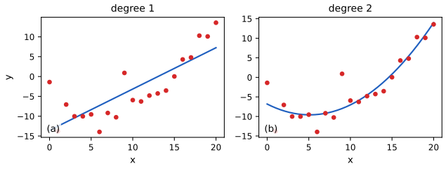
pp. 371–372 The standard model is \[ p(y\given\bm x,\bm\theta)=\mathcal N(y\given w_0+\bm w^\T\bm x,\sigma^2),\qquad \bm\theta=(w_0,\bm w,\sigma^2), \tag{11.1} \] with offset (bias, intercept) \(w_0\) and weights (regression coefficients) \(\bm w\). Absorbing the offset by prepending a 1 to \(\bm x\) lets us write \(\bm w^\T\bm x\) throughout. With one input this is simple linear regression \(f(x)=ax+b\); with several, multiple linear regression; with a vector response \(\bm y\in\R^J\) and independent components, multivariate linear regression \[ p(\bm y\given\bm x,\bm W)=\prod_{j=1}^J\mathcal N(y_j\given\bm w_j^\T\bm x,\sigma_j^2). \tag{11.2} \] Because the columns of the weight matrix do not interact, the multivariate problem is \(J\) separate univariate problems (Exercise 11.1 is a worked case). Replacing \(\bm x\) by a fixed feature vector \(\bm\phi(\bm x)\), \[ p(y\given\bm x,\bm\theta)=\mathcal N(y\given\bm w^\T\bm\phi(\bm x),\sigma^2), \tag{11.3} \] keeps the model linear in the parameters: polynomial regression uses \(\bm\phi(x)=[1,x,\dots,x^d]\) (Figure 11.1); Section 11.5 uses spline bases.
See also (companion): Bishop 3.1.1 for the same model with basis functions; the polynomial overfitting demo of Chapter 1.
11.2.2 Least squares estimation
pp. 372–376 The negative log likelihood is \[ \operatorname{NLL}(\bm w,\sigma^2)=-\sum_{n=1}^N\log\Big[\Big(\frac1{2\pi\sigma^2}\Big)^{1/2}\exp\Big(-\frac{(y_n-\bm w^\T\bm x_n)^2}{2\sigma^2}\Big)\Big]=\frac1{2\sigma^2}\sum_n(y_n-\hat y_n)^2+\frac N2\log(2\pi\sigma^2), \tag{11.5} \] with \(\hat y_n=\bm w^\T\bm x_n\). For fixed \(\sigma^2\) minimising it over \(\bm w\) is minimising \(\operatorname{RSS}(\bm w)=\frac12\|\bm X\bm w-\bm y\|_2^2\) (11.6); the variance is estimated afterwards (Section 11.2.3.6).
11.2.2.1 Ordinary least squares
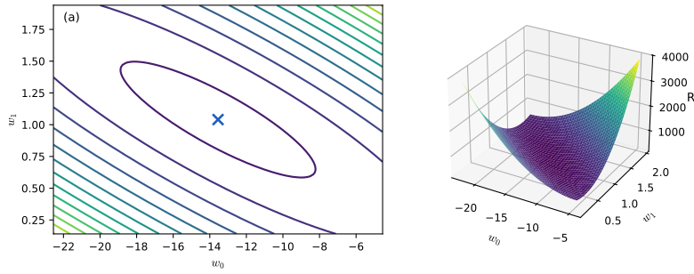
The gradient and Hessian of the RSS are \(\nabla\operatorname{RSS}=\bm X^\T\bm X\bm w-\bm X^\T\bm y\) (11.7) and \(\bm H=\bm X^\T\bm X\) (11.10). Setting the gradient to zero gives the normal equations \(\bm X^\T\bm X\bm w=\bm X^\T\bm y\) (11.8) and, when \(\bm X\) has full column rank, the ordinary least squares (OLS) solution \[ \hat{\bm w}=(\bm X^\T\bm X)^{-1}\bm X^\T\bm y=\bm X^\dagger\bm y, \tag{11.9} \] with \(\bm X^\dagger\) the left pseudo-inverse. Figure 11.2 shows the quadratic error surface for the straight-line fit of Figure 11.1a.
Filling the gap 11.2a: the normal equations, uniqueness, and the rank-deficient case pp. 373, (11.7)–(11.11)
Derivation
Gradient and Hessian. Expanding, \[ \operatorname{RSS}(\bm w)=\frac12\bm w^\T\bm X^\T\bm X\bm w-\bm w^\T\bm X^\T\bm y+\frac12\bm y^\T\bm y \], a quadratic with gradient \(\bm X^\T\bm X\bm w-\bm X^\T\bm y\) and constant Hessian \(\bm X^\T\bm X\). For any \(\bm v\) we have \(\bm v^\T\bm X^\T\bm X\bm v=\|\bm X\bm v\|_2^2\ge0\), so the RSS is convex, and any stationary point is a global minimiser.
Uniqueness. If the columns of \(\bm X\) are linearly independent then \(\bm X\bm v\ne\bm 0\) for every \(\bm v\ne\bm 0\), hence \(\bm v^\T\bm X^\T\bm X\bm v=\|\bm X\bm v\|^2>0\): the Hessian is positive definite, \(\bm X^\T\bm X\) is invertible, and the RSS is strictly convex with the unique minimiser (11.9). (The book writes "for any \(\bm v>0\)" in (11.11); the condition is \(\bm v\ne\bm 0\), not positivity of the entries.)
Rank-deficient case. If the columns are dependent (for example \(D>N\) or two identical features) the normal equations are still consistent, because \[ \bm X^\T\bm y\in\operatorname{range}(\bm X^\T)=\operatorname{range}(\bm X^\T\bm X) \]. The minimisers form the affine set \(\hat{\bm w}_0+\ker\bm X\), all with the same fit \(\bm X\hat{\bm w}\); the one of smallest norm is \(\bm X^\dagger\bm y\) with \(\bm X^\dagger\) the Moore–Penrose pseudo-inverse (computed by the SVD, Section 11.2.2.3). In that case individual coefficients are not identifiable, which is the theme of Section 11.7.6.
The variance does not matter for \(\bm w\). The NLL (11.5) depends on \(\sigma^2\) only through the factor \(1/(2\sigma^2)\) in front of the RSS, so \(\hat{\bm w}\) is the same for every \(\sigma^2>0\). \(\square\)
11.2.2.2 Geometric interpretation of least squares
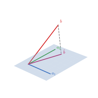
pp. 373–375 For \(N>D\) the system \(\bm X\bm w=\bm y\) is overdetermined. We look for \(\hat{\bm y}\in\operatorname{span}(\bm x_{:,1},\dots,\bm x_{:,D})\) closest to \(\bm y\) (11.12), \(\hat{\bm y}=\bm X\bm w\) (11.13). The residual must be orthogonal to every column, \(\bm x_{:,d}^\T(\bm y-\hat{\bm y})=0\), which is the normal equations again (11.14), and \[ \hat{\bm y}=\bm X(\bm X^\T\bm X)^{-1}\bm X^\T\bm y=\operatorname{Proj}(\bm X)\bm y, \tag{11.15,\ 11.16} \] the orthogonal projection onto the column space (the "hat matrix"); for a single column \(\bm x\) it is \(\bm x\,\bm x^\T\bm y/\bm x^\T\bm x\) (11.17).
Filling the gap 11.2b: the hat matrix, Pythagoras, and why the normal equations are avoided numerically pp. 374–375
Derivation
The projection property. Let \(\bm P=\bm X(\bm X^\T\bm X)^{-1}\bm X^\T\) (full column rank). Then \(\bm P^\T=\bm P\), and \[ \bm P^2=\bm X(\bm X^\T\bm X)^{-1}(\bm X^\T\bm X)(\bm X^\T\bm X)^{-1}\bm X^\T=\bm P \], so \(\bm P\) is an orthogonal projection; \(\bm P\bm X=\bm X\) shows it fixes the column space, and \(\bm P\bm z=\bm 0\) for \(\bm z\perp\operatorname{range}\bm X\). Its trace is \[ \operatorname{tr}\bm P=\operatorname{tr}((\bm X^\T\bm X)^{-1}\bm X^\T\bm X)=D \], the dimension of the range.
Closest point. For any \(\bm u\in\operatorname{range}(\bm X)\), \(\hat{\bm y}-\bm u\in\operatorname{range}(\bm X)\) is orthogonal to \(\bm y-\hat{\bm y}\), so \[ \|\bm y-\bm u\|^2=\|\bm y-\hat{\bm y}\|^2+\|\hat{\bm y}-\bm u\|^2\ge\|\bm y-\hat{\bm y}\|^2 \], with equality iff \(\bm u=\hat{\bm y}\). This is a proof of (11.12)–(11.14) that needs no calculus.
QR. Write the thin factorisation \(\bm X=\bm Q\bm R\) with \(\bm Q^\T\bm Q=\bm I_D\) and \(\bm R\) upper triangular and invertible (full rank). Then \(\bm X^\T\bm X=\bm R^\T\bm R\) and \(\bm X^\T\bm y=\bm R^\T\bm Q^\T\bm y\); multiplying the normal equations by \(\bm R^{-\T}\) gives \(\bm R\bm w=\bm Q^\T\bm y\), solved by back-substitution (11.19)–(11.21). Also \(\bm P=\bm Q\bm Q^\T\).
Conditioning. If \(\bm X=\bm U\bm S\bm V^\T\) then \(\bm X^\T\bm X=\bm V\bm S^2\bm V^\T\), so \(\kappa(\bm X^\T\bm X)=\kappa(\bm X)^2\): forming the normal equations squares the condition number and loses half the digits of precision, whereas QR and the SVD work with \(\kappa(\bm X)\). In the code, ols_normal, ols_qr and ols_svd agree on well-conditioned data (confirmed numerically) and diverge on nearly collinear data. \(\square\)
See also (companion): Bishop 3.1.2, geometry of least squares.
11.2.2.3 Algorithmic issues
pp. 375–376 Do not invert \(\bm X^\T\bm X\). The robust general method is the SVD (this is what the standard libraries call, via LAPACK's gelsd); for tall thin \(\bm X\) the QR factorisation of (11.19)–(11.21) is faster, and for huge sparse problems one can use iterative solvers (conjugate gradient, GMRES) that only need matrix–vector products. Standardise the inputs first (zero mean, unit variance), as in Equation (10.51), so that penalties and step sizes treat the features alike.
11.2.2.4 Weighted least squares
p. 376 With input-dependent noise (heteroskedastic regression), \(p(y\given\bm x)=\mathcal N(y\given\bm w^\T\bm x,\sigma^2(\bm x))\) (11.22), that is \(\mathcal N(\bm y\given\bm X\bm w,\bm\Lambda^{-1})\) with \(\bm\Lambda=\operatorname{diag}(1/\sigma^2(\bm x_n))\) (11.23), the MLE is the weighted least squares estimate \[ \hat{\bm w}=(\bm X^\T\bm\Lambda\bm X)^{-1}\bm X^\T\bm\Lambda\bm y. \tag{11.24} \]
Filling the gap 11.2c: derivation of weighted least squares p. 376, (11.24)
Derivation
With known variances the NLL is \[ \frac12\sum_n\lambda_n(y_n-\bm w^\T\bm x_n)^2+\mathrm{const}=\frac12(\bm X\bm w-\bm y)^\T\bm\Lambda(\bm X\bm w-\bm y)+\mathrm{const} \], with \(\lambda_n=1/\sigma^2(\bm x_n)\). Its gradient is \(\bm X^\T\bm\Lambda(\bm X\bm w-\bm y)\), so the weighted normal equations are \(\bm X^\T\bm\Lambda\bm X\bm w=\bm X^\T\bm\Lambda\bm y\), and \(\bm X^\T\bm\Lambda\bm X\succ0\) when the columns are independent and all \(\lambda_n>0\). Equivalently, weighted least squares is ordinary least squares on the rescaled data \((\sqrt{\lambda_n}\bm x_n,\sqrt{\lambda_n}y_n)\): points with small noise count more. The same formula with weights \(u_n\) that depend on the residuals is the engine of the IRLS algorithms for the Student and Huber fits in Section 11.6 (gap 11.6b). \(\square\)
11.2.3 Other approaches to computing the MLE
11.2.3.1 Solving for offset and slope separately
p. 376 Writing \(\bar{\bm x}\), \(\bar y\) for the sample means and \(\bm X_c,\bm y_c\) for the centred data, the offset and the weights can be solved separately: \[ \hat{\bm w}=(\bm X_c^\T\bm X_c)^{-1}\bm X_c^\T\bm y_c=\Big[\sum_n(\bm x_n-\bar{\bm x})(\bm x_n-\bar{\bm x})^\T\Big]^{-1}\Big[\sum_n(y_n-\bar y)(\bm x_n-\bar{\bm x})\Big],\qquad \hat w_0=\bar y-\bar{\bm x}^\T\hat{\bm w}. \tag{11.25, 11.26} \]
11.2.3.2 Simple linear regression (1d inputs)
pp. 377 For \(D=1\), \[ \hat w_1=\frac{\sum_n(x_n-\bar x)(y_n-\bar y)}{\sum_n(x_n-\bar x)^2}=\frac{C_{xy}}{C_{xx}}=\rho_{xy}\frac{\sigma_y}{\sigma_x},\qquad \hat w_0=\bar y-\hat w_1\bar x, \tag{11.27, 11.28} \] so the prediction is \(\hat y=\bar y+\rho_{xy}\sigma_y(x-\bar x)/\sigma_x\): go \(\rho\) times as many standard deviations from the mean of \(y\) as \(x\) is from the mean of \(x\) ("regression to the mean" when \(|\rho|<1\)).
11.2.3.3 Partial regression
p. 377 The simple slope is \(R_{YX}=\partial\E[Y\given X=x]/\partial x=C_{xy}/C_{xx}\) (11.29). With two inputs, the optimal coefficient of \(X_1\) is the partial regression coefficient \(R_{YX_1\cdot X_2}\), the slope of \(Y\) on \(X_1\) holding \(X_2\) fixed (11.30), and similarly in higher dimensions: \(\hat w_j\) is the change in the output per unit change of input \(j\) with the others held constant.
Filling the gap 11.2d: centring (11.25–11.26), simple regression (11.27–11.28), and partial regression (11.30) pp. 376–377
Derivation
Offset and slope separately. With the offset, \[ \operatorname{RSS}(w_0,\bm w)=\frac12\sum_n(y_n-w_0-\bm w^\T\bm x_n)^2 \]. Setting \(\partial/\partial w_0=0\) gives \(\sum_n(y_n-w_0-\bm w^\T\bm x_n)=0\), that is \(w_0=\bar y-\bar{\bm x}^\T\bm w\). Substituting, \[ y_n-w_0-\bm w^\T\bm x_n=(y_n-\bar y)-\bm w^\T(\bm x_n-\bar{\bm x}) \], so \(\operatorname{RSS}=\frac12\|\bm y_c-\bm X_c\bm w\|^2\): a least squares problem in the centred data with no offset, whose normal equations are (11.25). The two stages together give the joint minimum, since the first-order conditions are the same as for the joint problem. In particular the fitted line always passes through \((\bar{\bm x},\bar y)\).
Simple regression. For \(D=1\), \(\bm X_c^\T\bm X_c=\sum(x_n-\bar x)^2\) and \(\bm X_c^\T\bm y_c=\sum(x_n-\bar x)(y_n-\bar y)\), so (11.27) follows after dividing numerator and denominator by \(N\): \[ C_{xy}/C_{xx}=\rho_{xy}\sigma_x\sigma_y/\sigma_x^2=\rho_{xy}\sigma_y/\sigma_x \].
Partial regression (Frisch–Waugh–Lovell). Partition \(\bm X=[\bm x_1,\bm X_2]\) and \(\bm w=(w_1,\bm w_2)\). The normal equations read \(\bm x_1^\T\bm x_1w_1+\bm x_1^\T\bm X_2\bm w_2=\bm x_1^\T\bm y\) and \(\bm X_2^\T\bm x_1w_1+\bm X_2^\T\bm X_2\bm w_2=\bm X_2^\T\bm y\). The second gives \(\bm w_2=(\bm X_2^\T\bm X_2)^{-1}\bm X_2^\T(\bm y-\bm x_1w_1)\). Substituting in the first and writing \(\bm M_2=\bm I-\bm P_2\) for the projection onto the orthogonal complement of \(\operatorname{range}\bm X_2\): \[ \bm x_1^\T\bm M_2\bm x_1\,w_1=\bm x_1^\T\bm M_2\bm y\quad\Rightarrow\quad\hat w_1=\frac{(\bm M_2\bm x_1)^\T(\bm M_2\bm y)}{\|\bm M_2\bm x_1\|^2}, \] using \(\bm M_2^\T\bm M_2=\bm M_2\). So \(\hat w_1\) is the simple-regression slope of \(\bm y\) (or of \(\bm M_2\bm y\), the same thing) on the part of \(\bm x_1\) that is not linearly explained by the other inputs: this is what "holding \(X_2\) constant" means. When \(\E[Y\given\bm X]\) really is linear, \(\partial\E[Y\given X_1=x,X_2]/\partial x\) equals the coefficient and does not depend on the value of \(X_2\) (as the book notes). The partial coefficient differs from the simple slope \(C_{xy}/C_{xx}\) unless \(\bm x_1\perp\bm X_2\) after centring. A numerical confirmation is in the code. \(\square\)
11.2.3.4 Recursively computing the MLE
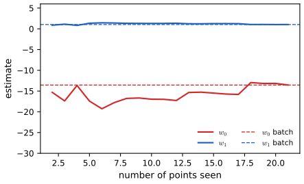
pp. 377–378 For data that arrive in a stream, keep the sufficient statistics (means \(\bar x^{(n)},\bar y^{(n)}\) and the second moments \(C^{(n)}_{xx},C^{(n)}_{xy},C^{(n)}_{yy}\), defined with divisor \(n\); (11.33)–(11.34)) and update them online: \[ \bar x^{(n+1)}=\bar x^{(n)}+\frac{x_{n+1}-\bar x^{(n)}}{n+1},\qquad C^{(n+1)}_{xy}=\frac1{n+1}\Big[x_{n+1}y_{n+1}+nC^{(n)}_{xy}+n\bar x^{(n)}\bar y^{(n)}-(n+1)\bar x^{(n+1)}\bar y^{(n+1)}\Big]. \tag{11.35, 11.40} \] The estimate \(\hat w_1=C_{xy}/C_{xx}\), \(\hat w_0=\bar y-\hat w_1\bar x\) is then available after every point (Figure 11.4). For \(D>1\) the book recommends stochastic gradient descent, the least mean squares (LMS) algorithm of Section 8.4.2.
Filling the gap 11.2e: the recursion (11.36–11.40), the matching update for \(C_{xx}\), and LMS pp. 377–378
Derivation
Rewriting \(C_{xy}\). Expanding \(\sum_i(x_i-\bar x)(y_i-\bar y)=\sum_ix_iy_i-n\bar x\bar y\) (this is what (11.36)–(11.38) do in several lines: the cross terms \(-\bar x\sum y_i-\bar y\sum x_i\) equal \(-2n\bar x\bar y\), and \(\sum\bar x\bar y=n\bar x\bar y\)), we get \(\sum_{i\le n}x_iy_i=nC_{xy}^{(n)}+n\bar x^{(n)}\bar y^{(n)}\) (11.39). Adding the new term and recentring with the updated means gives (11.40): \[ C^{(n+1)}_{xy}=\frac1{n+1}[x_{n+1}y_{n+1}+\sum_{i\le n}x_iy_i-(n+1)\bar x^{(n+1)}\bar y^{(n+1)}] \].
The \(C_{xx}\) update (the book says "in a similar manner") is the same computation with \(y\) replaced by \(x\): \[ C^{(n+1)}_{xx}=\frac1{n+1}[x_{n+1}^2+nC^{(n)}_{xx}+n(\bar x^{(n)})^2-(n+1)(\bar x^{(n+1)})^2] \].
An equivalent numerically friendlier form. With \(\delta_x=x_{n+1}-\bar x^{(n)}\) and \(\delta_y=y_{n+1}-\bar y^{(n)}\), one checks that \((n+1)C^{(n+1)}_{xy}=nC^{(n)}_{xy}+\frac n{n+1}\delta_x\delta_y\) (Welford's update, which avoids subtracting two large nearly equal numbers). Proof: \(\bar x^{(n+1)}=\bar x^{(n)}+\delta_x/(n+1)\), and writing \(x_i-\bar x^{(n+1)}=(x_i-\bar x^{(n)})-\delta_x/(n+1)\) for \(i\le n\) and \(x_{n+1}-\bar x^{(n+1)}=\frac n{n+1}\delta_x\), the sum of products is \[ \sum_{i\le n}(x_i-\bar x^{(n)})(y_i-\bar y^{(n)})+n\frac{\delta_x\delta_y}{(n+1)^2}+\frac{n^2}{(n+1)^2}\delta_x\delta_y \] (the cross terms vanish because the deviations from the old mean sum to zero), and \(\frac{n+n^2}{(n+1)^2}=\frac n{n+1}\).
Exactness. The recursion computes exactly the batch sufficient statistics, so the online estimate after \(n\) points equals the OLS estimate on those \(n\) points (it is undefined while \(C_{xx}=0\), that is for the first point). In the code, online_simple reproduces np.polyfit after every step (confirmed numerically); the estimate wanders at the start and settles on the batch line (Figure 11.4).
LMS. For \(D>1\) the stochastic gradient of \(\frac12(y_n-\bm w^\T\bm x_n)^2\) is \(-(y_n-\bm w^\T\bm x_n)\bm x_n\), giving \(\bm w\leftarrow\bm w+\eta_n(y_n-\bm w^\T\bm x_n)\bm x_n\). It needs \(O(D)\) memory and time per point but converges only with a decaying step size. The exact alternative, recursive least squares, updates \((\bm X^\T\bm X)^{-1}\) by the Sherman–Morrison formula and is \(O(D^2)\) per point. \(\square\)
See also (companion): Bishop 3.1.3, sequential learning.
11.2.3.5 Deriving the MLE from a generative perspective
pp. 378–379 Fit a joint Gaussian \(p(\bm x,y)\) by maximum likelihood (empirical means and covariances, (11.42)–(11.45)) and condition: \[ \E[y\given\bm x]=\mu_y+\bm\Sigma_{xy}^\T\bm\Sigma_{xx}^{-1}(\bm x-\bm\mu_x) \] (11.46), that is \(w_0=\bar y-\bm w^\T\bar{\bm x}\) (11.47) and \[ \bm w=\bm\Sigma_{xx}^{-1}\bm\Sigma_{xy}=(\bm X_c^\T\bm X_c)^{-1}\bm X_c^\T\bm y_c \] (11.48). This is the same as the discriminative OLS fit, but only for Gaussian models.
11.2.3.6 Deriving the MLE for \(\sigma^2\)
pp. 379–380 After estimating \(\hat{\bm w}\), \(\hat\sigma^2_{\rm mle}=\frac1N\sum_n(y_n-\bm x_n^\T\hat{\bm w})^2\) (11.49), the mean squared residual.
Filling the gap 11.2f: the generative route and \(\hat\sigma^2_{\rm mle}\), with its bias pp. 378–380, (11.42)–(11.49)
Derivation
The two routes agree. The MLE of a multivariate normal is the empirical mean and the \(1/N\) covariance (Section 4.2.6, reproduced in gap 4.3), giving (11.42)–(11.45). The conditioning formula for Gaussians (3.28) then yields (11.46). With \(\bm\Sigma_{xx}=\frac1N\bm X_c^\T\bm X_c\) and \(\bm\Sigma_{xy}=\frac1N\bm X_c^\T\bm y_c\) the factors \(1/N\) cancel in \(\bm\Sigma_{xx}^{-1}\bm\Sigma_{xy}\), giving (11.48), and (11.47) is (11.26). So the conditional of the fitted joint equals the fitted conditional. The reason this works for Gaussians is that the maximum likelihood estimate of a function of the parameters is the function of the MLE (invariance), and the Gaussian joint factorises into a marginal of \(\bm x\) and a conditional of \(y\) with variationally independent parameters; for other joint models the two fits differ (Section 9.4).
Variance. With \(s=\sigma^2\) and \(\operatorname{SS}=\sum_n(y_n-\bm x_n^\T\hat{\bm w})^2\), \(g(s)=\frac N2\log(2\pi s)+\operatorname{SS}/(2s)\) has \[ g'(s)=\frac N{2s}-\frac{\operatorname{SS}}{2s^2}=\frac{Ns-\operatorname{SS}}{2s^2} \], negative for \(s<\operatorname{SS}/N\) and positive after, so the unique global minimiser is \(\hat s=\operatorname{SS}/N\) (11.49). (The joint maximisation can be done in this order because for every \(s\) the minimiser over \(\bm w\) is the same \(\hat{\bm w}\).)
Bias. If the model is correct, \(\bm y-\hat{\bm y}=(\bm I-\bm P)\bm\varepsilon\) with \(\bm\varepsilon\sim\mathcal N(\bm 0,\sigma^2\bm I)\), so \[ \E\|\bm y-\hat{\bm y}\|^2=\sigma^2\operatorname{tr}(\bm I-\bm P)=\sigma^2(N-D) \] (gap 11.2b). Hence \(\E[\hat\sigma^2_{\rm mle}]=\sigma^2(N-D)/N\): the MLE underestimates the variance because \(D\) degrees of freedom were spent on the fit, and \(\operatorname{RSS}/(N-D)\) is unbiased. \(\square\)
11.2.4 Measuring goodness of fit
11.2.4.1 Residual plots
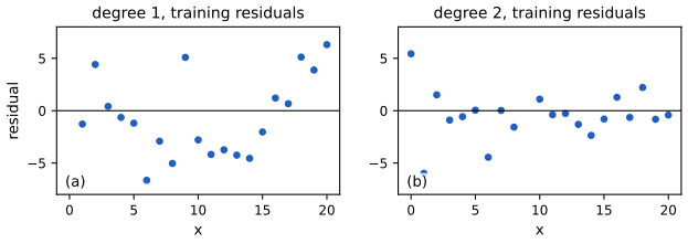
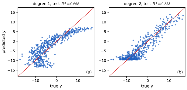
pp. 380–381 For one-dimensional inputs plot the residuals \(r_n=y_n-\hat y_n\) against \(x_n\): under the model they are a patternless cloud around 0. Curvature signals lack of fit (Figure 11.5a, the straight line); a good model leaves no structure (11.5b). For several inputs plot the predictions against the true values; a good model lies on the diagonal (Figure 11.6).
11.2.4.2 Prediction accuracy and \(R^2\)
p. 381 The RSS, the root mean squared error \(\operatorname{RMSE}=\sqrt{\operatorname{RSS}/N}\) (11.50), and the coefficient of determination \[ R^2=1-\frac{\sum_n(\hat y_n-y_n)^2}{\sum_n(\bar y-y_n)^2}=1-\frac{\operatorname{RSS}}{\operatorname{TSS}} \tag{11.51} \] measure fit; \(R^2=0\) means no better than predicting \(\bar y\), \(R^2=1\) a perfect fit.
Filling the gap 11.2g: \(R^2\in[0,1]\) on the training set, \(R^2=\operatorname{corr}(y,\hat y)^2\), and \(R^2\) on test data p. 381, (11.51)
Derivation
Assume the fit includes an offset, so the all-ones vector \(\bm 1\in\operatorname{range}\bm X\). Then \(\bar{\hat y}=\bar y\) (the residuals are orthogonal to \(\bm 1\) and so sum to zero), and \(\hat{\bm y}-\bar y\bm 1\in\operatorname{range}\bm X\) is orthogonal to the residual \(\bm y-\hat{\bm y}\). Pythagoras for \(\bm y-\bar y\bm 1=(\bm y-\hat{\bm y})+(\hat{\bm y}-\bar y\bm 1)\) gives \[ \operatorname{TSS}=\operatorname{RSS}+\operatorname{ESS},\qquad\operatorname{ESS}=\sum_n(\hat y_n-\bar y)^2, \] so \(R^2=\operatorname{ESS}/\operatorname{TSS}\in[0,1]\). Moreover \[ \sum_n(y_n-\bar y)(\hat y_n-\bar y)=\operatorname{ESS}+\sum(y_n-\hat y_n)(\hat y_n-\bar y)=\operatorname{ESS} \], so the squared sample correlation of \(y\) and \(\hat y\) is \[ \operatorname{ESS}^2/(\operatorname{TSS}\cdot\operatorname{ESS})=R^2 \]. For simple regression \(\hat y-\bar y=\hat w_1(x-\bar x)\), so \(R^2=\rho_{xy}^2\) (11.27).
On test data (or without an offset) the decomposition fails and \(R^2\) computed by (11.51) can be negative: a model that predicts worse than the training mean of the response has \(\operatorname{RSS}_{\rm test}>\operatorname{TSS}_{\rm test}\). The \(R^2\) values in Figure 11.6 are of this kind. Training \(R^2\) never decreases when a feature is added, so it cannot choose the model size. \(\square\)
11.3 Ridge regression
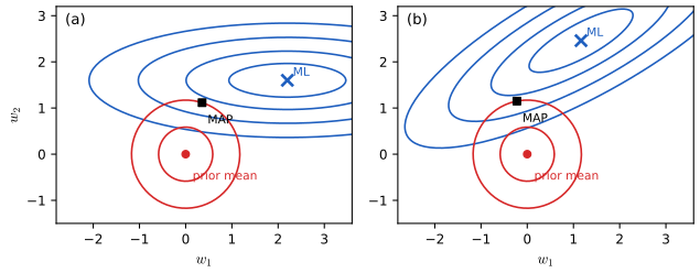
p. 381 Maximum likelihood can overfit (Section 1.2.2.2). MAP estimation with a zero-mean Gaussian prior \(p(\bm w)=\mathcal N(\bm w\given\bm 0,\tau^2\bm I)\) is ridge regression: \[ \hat{\bm w}_{\rm map}=\argmin\ \frac1{2\sigma^2}(\bm y-\bm X\bm w)^\T(\bm y-\bm X\bm w)+\frac1{2\tau^2}\bm w^\T\bm w=\argmin\ \operatorname{RSS}(\bm w)+\lambda\|\bm w\|_2^2, \tag{11.52, 11.53} \] where \(\lambda=\sigma^2/\tau^2\) measures the prior strength; \(\ell_2\) regularisation or weight decay. The offset is not penalised (Exercise 11.2).
11.3.1 Computing the MAP estimate
p. 382 The penalised objective is \[ J(\bm w)=(\bm y-\bm X\bm w)^\T(\bm y-\bm X\bm w)+\lambda\|\bm w\|_2^2 \] (11.55) with gradient \(2(\bm X^\T\bm X\bm w-\bm X^\T\bm y+\lambda\bm w)\) (11.56) and solution \[ \hat{\bm w}_{\rm map}=(\bm X^\T\bm X+\lambda\bm I_D)^{-1}\bm X^\T\bm y. \tag{11.57} \]
Filling the gap 11.3a: ridge as MAP, existence for every \(\lambda>0\), and the virtual-data trick pp. 381–382, (11.52)–(11.64)
Derivation
MAP. \[ -\log p(\bm w\given\mathcal D)=\frac1{2\sigma^2}\|\bm y-\bm X\bm w\|^2+\frac1{2\tau^2}\|\bm w\|^2+\mathrm{const}=\frac1{2\sigma^2}\big[\|\bm y-\bm X\bm w\|^2+\lambda\|\bm w\|^2\big]+\mathrm{const} \] with \(\lambda=\sigma^2/\tau^2\); so the MAP minimises the unhalved objective (11.55). (With \(\operatorname{RSS}\) defined with the factor \(\frac12\) as in (11.6) the equivalent statement is \(\operatorname{RSS}+\frac\lambda2\|\bm w\|^2\); the book's (11.53) mixes the two conventions, see the notes.)
Existence. The Hessian of (11.55) is \(2(\bm X^\T\bm X+\lambda\bm I)\succeq2\lambda\bm I\succ0\), so \(J\) is strongly convex, has a unique minimiser for every \(\lambda>0\) even if \(\bm X^\T\bm X\) is singular (\(D>N\) or collinear features), and (11.57) is its closed form. As \(\lambda\to0\) it tends to the minimum-norm least squares solution \(\bm X^\dagger\bm y\); as \(\lambda\to\infty\) it tends to \(\bm 0\).
Virtual data. Let \[ \tilde{\bm X}=\begin{bmatrix}\bm X/\sigma\\ \sqrt{\bm\Lambda}\end{bmatrix} \], \(\tilde{\bm y}=\begin{bmatrix}\bm y/\sigma\\ \bm 0\end{bmatrix}\) with \(\bm\Lambda=\sqrt{\bm\Lambda}\sqrt{\bm\Lambda}^\T\) the prior precision (here \(\bm\Lambda=\tau^{-2}\bm I\)). Then \[ \|\tilde{\bm y}-\tilde{\bm X}\bm w\|^2=\|\frac1\sigma(\bm y-\bm X\bm w)\|^2+\|\sqrt{\bm\Lambda}\bm w\|^2=\frac1{\sigma^2}\|\bm y-\bm X\bm w\|^2+\bm w^\T\bm\Lambda\bm w \], which is twice the negative log posterior up to a constant (11.59)–(11.63): ridge is OLS on the data augmented by \(D\) pseudo-observations that "observe" \(\bm w\) to be 0 with precision \(\bm\Lambda\). So the QR solver applies: factor \(\tilde{\bm X}=\tilde{\bm Q}\tilde{\bm R}\), cost \(O((N+D)D^2)\), and no matrix inversion (11.64); this is ridge_qr in the code. \(\square\)
11.3.1.2 Solving using SVD
p. 383 When \(D>N\) (the usual case for ridge) use the thin SVD \(\bm X=\bm U\bm S\bm V^\T\) with \(\bm V\in\R^{D\times N}\), \(\bm U,\bm S\in\R^{N\times N}\), put \(\bm R=\bm U\bm S\), and \[ \hat{\bm w}_{\rm map}=\bm V(\bm R^\T\bm R+\lambda\bm I_N)^{-1}\bm R^\T\bm y, \tag{11.65} \] the ridge solution in the \(N\)-dimensional coordinates \(\bm r_n=\bm V^\T\bm x_n\); cost \(O(DN^2)\), cheaper than \(O(D^3)\).
11.3.2 Connection between ridge regression and PCA
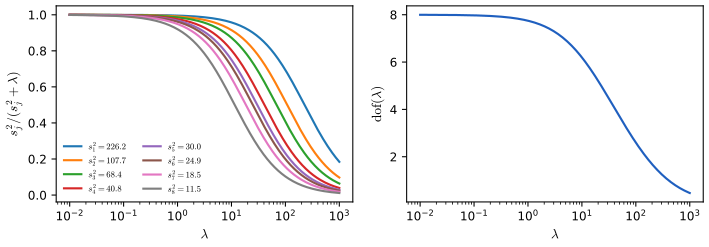
pp. 383–384 The ridge predictions on the training set are \[ \hat{\bm y}=\bm X\hat{\bm w}_{\rm map}=\bm U\bm S\bm V^\T\bm V(\bm S^2+\lambda\bm I)^{-1}\bm S\bm U^\T\bm y=\sum_j\bm u_j\frac{\sigma_j^2}{\sigma_j^2+\lambda}\bm u_j^\T\bm y \tag{11.66–11.69} \] with singular values \(\sigma_j\), whereas least squares gives \(\sum_j\bm u_j\bm u_j^\T\bm y\) (11.70): ridge shrinks the component along \(\bm u_j\) by \(\sigma_j^2/(\sigma_j^2+\lambda)\), little for directions of large variance, a lot for those of small variance. The effective number of degrees of freedom is \[ \operatorname{dof}(\lambda)=\sum_j\frac{\sigma_j^2}{\sigma_j^2+\lambda}, \tag{11.71} \] equal to \(D\) at \(\lambda=0\) and tending to 0 as \(\lambda\to\infty\). Under a flat prior \[ \operatorname{cov}[\bm w\given\mathcal D]\propto(\bm X^\T\bm X)^{-1} \] (Section 11.7), so the directions in which \(\bm w\) is least well determined are those of the smallest singular values, which ridge shrinks most (Figure 11.7). Principal components regression instead keeps the top \(K\) directions and discards the rest entirely, which predicts worse than the soft weighting of ridge.
Filling the gap 11.3b: the SVD form of ridge, shrinkage factors and the degrees of freedom pp. 383–384, (11.65)–(11.71)
Derivation
(11.65). The push-through identity \[ (\bm X^\T\bm X+\lambda\bm I_D)\bm X^\T=\bm X^\T(\bm X\bm X^\T+\lambda\bm I_N) \] (expand both sides) gives \[ (\bm X^\T\bm X+\lambda\bm I_D)^{-1}\bm X^\T=\bm X^\T(\bm X\bm X^\T+\lambda\bm I_N)^{-1} \]. With \(\bm X=\bm U\bm S\bm V^\T\) (\(N\le D\), \(\bm U\) orthogonal, \(\bm V^\T\bm V=\bm I_N\)), \(\bm X\bm X^\T=\bm U\bm S^2\bm U^\T\), and \[ \bm X^\T(\bm X\bm X^\T+\lambda\bm I)^{-1}=\bm V\bm S\bm U^\T\bm U(\bm S^2+\lambda\bm I)^{-1}\bm U^\T=\bm V\bm S(\bm S^2+\lambda\bm I)^{-1}\bm U^\T \]. Since \(\bm R^\T\bm R=\bm S^2\) and \(\bm R^\T=\bm S\bm U^\T\), this is (11.65). (For \(N>D\) the same computation with the thin SVD of \(\bm X\) gives the same result with \(D\) singular values.)
Coordinates along the principal directions. Reading the result in the basis \(\bm v_j\): \[ \bm v_j^\T\hat{\bm w}_{\rm ridge}=\frac{\sigma_j}{\sigma_j^2+\lambda}\bm u_j^\T\bm y=\frac{\sigma_j^2}{\sigma_j^2+\lambda}\cdot\frac{\bm u_j^\T\bm y}{\sigma_j}=\frac{\sigma_j^2}{\sigma_j^2+\lambda}\,\bm v_j^\T\hat{\bm w}_{\rm ols} \]: each OLS coordinate is multiplied by the factor \(d_j(\lambda)=\sigma_j^2/(\sigma_j^2+\lambda)\in(0,1)\), decreasing in \(\lambda\) and increasing in \(\sigma_j\) (Figure 11.S2). Then \[ \hat{\bm y}=\bm X\hat{\bm w}=\sum_j\sigma_j\bm u_j(\bm v_j^\T\hat{\bm w}) \] gives (11.69).
Degrees of freedom. The map \(\bm y\mapsto\hat{\bm y}\) is linear with matrix \(\bm H_\lambda=\bm U\operatorname{diag}(d_j)\bm U^\T\), and \[ \operatorname{tr}\bm H_\lambda=\sum_jd_j=\operatorname{dof}(\lambda) \] (11.71). For OLS \(\bm H_0=\bm P\) has trace \(D\); the trace is the natural generalisation of the number of free parameters, because for a linear smoother with independent noise \[ \sum_n\operatorname{cov}[\hat y_n,y_n]=\sigma^2\operatorname{tr}\bm H_\lambda \]. That is the sense of "effective": it enters Mallows' \(C_p\) and AIC in the same way as the parameter count.
Why the small directions are shrunk. Under the likelihood alone \(\bm w\) has covariance \(\sigma^2(\bm X^\T\bm X)^{-1}=\sigma^2\bm V\bm S^{-2}\bm V^\T\): the variance of the coordinate along \(\bm v_j\) is \(\sigma^2/\sigma_j^2\), large when \(\sigma_j\) is small. A Gaussian prior of variance \(\tau^2\) combines with it by precision weighting, giving posterior mean weight \[ \frac{\sigma_j^2/\sigma^2}{\sigma_j^2/\sigma^2+1/\tau^2}=d_j(\lambda) \] on the data estimate and \(1-d_j\) on the prior mean 0, which is the same factor with \(\lambda=\sigma^2/\tau^2\). \(\square\)
See also (companion): ESL 3.4.1, ridge regression and the ridge and SVD demo; Bishop 3.1.4.
11.3.3 Choosing the strength of the regularizer
pp. 384–385 Choose \(\lambda\) by cross-validation (Section 4.5.5.2), warm-starting from the solution at the previous (larger) \(\lambda\); the curve of solutions \(\hat{\bm w}(\lambda)\) is the regularisation path (Figure 11.10a). The empirical-Bayes alternative maximises the marginal likelihood \(p(\mathcal D\given\lambda)\): it needs one fit rather than \(K\), and it is smooth in \(\lambda\), so gradient methods apply (Section 11.7.7 and Bishop 3.5).
11.4 Lasso regression
p. 385 A Gaussian prior makes the weights small; sometimes we want them exactly zero, so that \(\hat{\bm w}\) is sparse (few non-zero entries, the \(\ell_0\) norm \(\|\bm w\|_0=\sum_d\mathbb I(|w_d|>0)\), (11.72)) and the model performs feature selection: if \(w_d=0\) the feature \(x_d\) is ignored.
11.4.1 MAP estimation with a Laplace prior (\(\ell_1\) regularization)
p. 385 With independent Laplace priors \[ p(\bm w\given\lambda)=\prod_d\operatorname{Laplace}(w_d\given0,1/\lambda)\propto\prod_de^{-\lambda|w_d|} \] (11.73), where \(\operatorname{Laplace}(w\given\mu,b)=\frac1{2b}\exp(-|w-\mu|/b)\) (11.74), the penalised negative log likelihood is \[ \operatorname{PNLL}(\bm w)=\|\bm X\bm w-\bm y\|_2^2+\lambda\|\bm w\|_1,\qquad\|\bm w\|_1=\sum_d|w_d|, \tag{11.75} \] the lasso ("least absolute shrinkage and selection operator", Tibshirani 1996). For the \(q\)-norm \(\|\bm w\|_q=(\sum_d|w_d|^q)^{1/q}\) (11.76) the case \(q<1\) is even sparser but non-convex; the \(\ell_1\) norm is the tightest convex relaxation of \(\|\bm w\|_0\).
A word on the factor 2. The objective (11.75) uses the unhalved sum of squares, while the coordinate update, the threshold \(\lambda\), and the critical value \(\lambda_{\max}\) in (11.81)–(11.90) correspond to the halved loss \(\frac12\|\bm y-\bm X\bm w\|^2+\lambda\|\bm w\|_1\). The two differ by \(\lambda\mapsto\lambda/2\). These notes use the halved form below (the one for which \(\lambda_{\max}=\|\bm X^\T\bm y\|_\infty\) and the soft threshold is exactly \(\lambda\)); Section Notes on the book shows the discrepancy numerically.
Filling the gap 11.4a: the \(\ell_q\) claims, the Lagrangian form, and convexity pp. 385–386, (11.76)–(11.80)
Derivation
\(q\ge1\) convex, \(q<1\) not. For \(q\ge1\), \(\|\cdot\|_q\) is a norm (Minkowski's inequality), hence convex. For \(0<q<1\) the set \(\{\bm w:\sum_d|w_d|^q\le1\}\) is not convex: \(\bm e_1\) and \(\bm e_2\) are in it, but their midpoint \((\frac12,\frac12)\) has \(\sum|w_d|^q=2\cdot2^{-q}=2^{1-q}>1\). So \(\ell_q\) regularisation with \(q<1\) gives non-convex problems with possibly many local minima; \(q=1\) is the smallest exponent that keeps convexity, and the \(\ell_1\) unit ball is exactly the convex hull of the \(\ell_q\) unit ball for \(q<1\): the \(\ell_q\) ball contains \(\pm\bm e_d\), whose hull is the \(\ell_1\) ball, and lies inside it because \(|w_d|\le|w_d|^q\) when \(|w_d|\le1\) gives \(\sum|w_d|\le\sum|w_d|^q\le1\). This is the precise sense of "tightest convex relaxation".
The limit \(q\to0\). It is the sum \(\sum_d|w_d|^q\), not the norm with the root \(1/q\), that tends to the number of non-zeros: \(|w_d|^q\to\mathbb I(w_d\ne0)\). The quantity \(\|\bm w\|_q=(\sum|w_d|^q)^{1/q}\) of (11.76) diverges as \(q\to0\) when \(\bm w\) has two or more non-zero entries (for \(k\) non-zero entries it behaves like \(k^{1/q}\)). Also \(\|\cdot\|_q\) with \(q<1\) is only a quasi-norm. The statement (11.77) is meant for the former quantity.
Penalised and constrained forms. Let \(f\) be convex and \(\hat{\bm w}_\lambda\) minimise \(f(\bm w)+\lambda\|\bm w\|_1\); put \(B=\|\hat{\bm w}_\lambda\|_1\). If some \(\bm w\) with \(\|\bm w\|_1\le B\) had \(f(\bm w)<f(\hat{\bm w}_\lambda)\), then \(f(\bm w)+\lambda\|\bm w\|_1<f(\hat{\bm w}_\lambda)+\lambda B\), a contradiction; so \(\hat{\bm w}_\lambda\) solves (11.79) with this \(B\). Conversely, for \(0<B<\|\hat{\bm w}_{\rm mle}\|_1\) the constraint is active and Lagrange duality (Slater's condition holds: \(\bm w=\bm 0\) is strictly feasible) gives a multiplier \(\lambda\ge0\) for which the constrained solution minimises the penalised objective. Small \(B\) corresponds to large \(\lambda\) and vice versa. The same argument with \(\|\bm w\|_2^2\) relates (11.80) to ridge. \(\square\)
11.4.2 Why does \(\ell_1\) regularization yield sparse solutions?
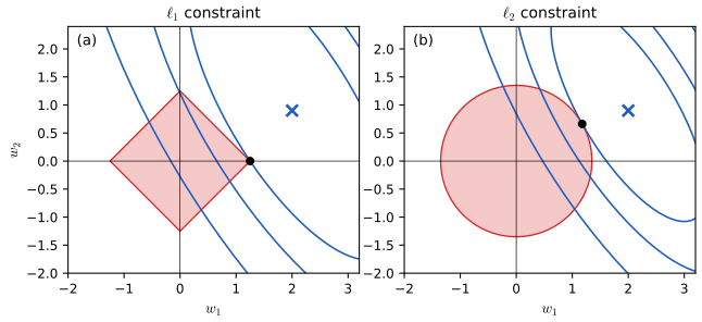
pp. 386–387 The lasso minimises \(\operatorname{NLL}(\bm w)+\lambda\|\bm w\|_1\) (11.78), the Lagrangian of \(\min\operatorname{NLL}(\bm w)\) subject to \(\|\bm w\|_1\le B\) (11.79); ridge has the constraint \(\|\bm w\|_2^2\le B\) (11.80). The constrained optimum is where the lowest level set of the NLL touches the constraint set (Figure 11.8). The \(\ell_2\) ball is smooth and can be touched anywhere; the \(\ell_1\) ball has corners on the coordinate axes, which stick out and are the most likely points of contact, especially in high dimension. The corners are the sparse points.
See also (companion): ESL 3.4.2, the lasso, 3.4.3, subset selection, ridge and the lasso compared; the l1-l2 paths demo.
11.4.3 Hard vs soft thresholding
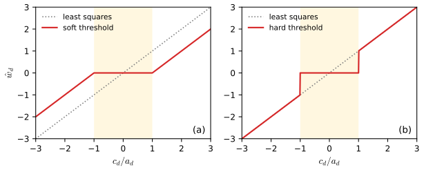
pp. 387–389 Write the squared-error part as a function of one coordinate with the others fixed. With \(a_d=\sum_nx_{nd}^2\) and \[ c_d=\sum_nx_{nd}(y_n-\bm w_{-d}^\T\bm x_{n,-d})=\bm x_{:,d}^\T\bm r_{-d} \], the derivative of the smooth part is \(a_dw_d-c_d\) (11.81)–(11.83), where \(c_d\) measures how well feature \(d\) correlates with the residual \(\bm r_{-d}=\bm y-\bm X_{:,-d}\bm w_{-d}\) of all the others. The unpenalised optimum is \(w_d=c_d/a_d\) (11.84), the orthogonal projection of the residual on the column. With the \(\ell_1\) term, \(\partial_{w_d}L=(a_dw_d-c_d)+\lambda\,\partial|w_d|\) is a set at \(w_d=0\) (11.85, 11.86), and the root of the subgradient condition is \[ \hat w_d(c_d)=\begin{cases}(c_d+\lambda)/a_d&c_d<-\lambda\\0&c_d\in[-\lambda,\lambda]\\(c_d-\lambda)/a_d&c_d>\lambda\end{cases}=\operatorname{SoftThreshold}\Big(\frac{c_d}{a_d},\frac\lambda{a_d}\Big), \tag{11.87, 11.88} \] with \[ \operatorname{SoftThreshold}(x,\delta)=\operatorname{sign}(x)(|x|-\delta)_+ \] (11.89). Hard thresholding sets \(w_d=0\) on \([-\lambda,\lambda]\) but leaves larger values unshrunk (Figure 11.9). Soft thresholding shifts every coefficient by \(\lambda\), so the lasso is biased; debiasing re-fits the selected coefficients by least squares.
Filling the gap 11.4b: the one-dimensional lasso problem, soft thresholding and the coordinate update pp. 387–388, (11.81)–(11.89), Exercise 11.3
Derivation
The partial derivative. Split \(\bm X\bm w=\bm x_{:,d}w_d+\bm X_{:,-d}\bm w_{-d}\); then \[ \frac12\|\bm y-\bm X\bm w\|^2=\frac12\|\bm r_{-d}-\bm x_{:,d}w_d\|^2=\frac12a_dw_d^2-c_dw_d+\frac12\|\bm r_{-d}\|^2 \] with \(\bm r_{-d}=\bm y-\bm X_{:,-d}\bm w_{-d}\), so the derivative with respect to \(w_d\) is \(a_dw_d-c_d\) (11.81). (With the unhalved \(\|\cdot\|^2\) both \(a_d\) and \(c_d\) double: Exercise 11.3 gives \(a_k=2\|\bm x_{:,k}\|^2\), \(c_k=2\bm x_{:,k}^\T\bm r_k\).)
One-dimensional lasso. Minimise \(h(w)=\frac12aw^2-cw+\lambda|w|\) with \(a>0\), \(\lambda\ge0\). It is strictly convex, so the minimiser is unique and is characterised by \(0\in\partial h(w)=aw-c+\lambda\,\partial|w|\), where \(\partial|w|=\{\operatorname{sign}w\}\) for \(w\ne0\) and \([-1,1]\) at 0. If \(w>0\): \(aw-c+\lambda=0\Rightarrow w=(c-\lambda)/a\), consistent iff \(c>\lambda\). If \(w<0\): \(w=(c+\lambda)/a\), consistent iff \(c<-\lambda\). If \(w=0\): need \(c\in[-\lambda,\lambda]\). The three cases are exclusive and exhaustive, giving (11.87); in closed form \(\hat w=\operatorname{sign}(c)(|c|-\lambda)_+/a\), which is (11.88) because \[ \operatorname{SoftThreshold}(c/a,\lambda/a)=\operatorname{sign}(c)(|c|/a-\lambda/a)_+ \].
Coordinate descent. Cycling through \(d=1,\dots,D\) and applying this update with the current residual is the shooting algorithm (Algorithm 11.1, below). The objective is smooth plus a separable non-smooth term, for which cyclic coordinate descent converges to a global minimum (Tseng 2001). Each update decreases the objective, and the iterates satisfy the KKT conditions of gap 11.4c in the limit (confirmed numerically against scikit-learn).
Soft against hard. Soft thresholding is the proximal operator of \(\lambda|\cdot|\) (it is the solution of \(\min_w\frac12(w-z)^2+\lambda|w|\); take \(a=1\), \(c=z\)); hard thresholding \(z\,\mathbb I(|z|>t)\) is the solution of the same problem with the penalty \(\lambda\mathbb I(w\ne0)\), \(t=\sqrt{2\lambda}\): non-zero \(w=z\) costs \(\lambda\), zero costs \(\frac12z^2\), and the cheaper is chosen. \(\square\)
11.4.4 Regularization path
pp. 389–390 At \(\lambda=0\) we get the dense OLS solution; as \(\lambda\) grows \(\hat{\bm w}(\lambda)\) tends to get sparser, and beyond the critical value \[ \lambda_{\max}=\max_d|\nabla_{w_d}\operatorname{NLL}(\bm 0)|=\max_d|\bm y^\T\bm x_{:,d}|=\|\bm X^\T\bm y\|_\infty \tag{11.90} \] it is exactly zero. Equivalently, in terms of a bound \(B\) on \(\|\bm w\|_1\), \(\hat{\bm w}=\bm 0\) at \(B=0\) and the solution is the OLS one for \(B\ge\|\hat{\bm w}_{\rm mle}\|_1\). Plotting the coefficients against \(\lambda\) (or \(B\)) gives the regularisation path (Figure 11.10b for the prostate data, Hastie et al. 2009); for ridge all coefficients are non-zero for every finite \(\lambda\) (11.10a). The lasso path is piecewise linear in \(\lambda\) (Efron et al. 2004): at a finite number of critical values the active set changes and in between each non-zero coefficient moves linearly. Table 11.1 lists the coefficients at the critical values; the last row is OLS. If \(D>N\) the lasso has at most \(N\) non-zero coefficients along its path (before the OLS solution of minimal \(\ell_1\) norm); the elastic net (Section 11.4.8) can go beyond \(N\).
Filling the gap 11.4c: optimality conditions, \(\lambda_{\max}\), and uniqueness p. 389, (11.90)
Derivation
The lasso objective \(F(\bm w)=\frac12\|\bm y-\bm X\bm w\|^2+\lambda\|\bm w\|_1\) is convex, so \(\bm w^\star\) is a minimiser iff \[ \bm 0\in\partial F(\bm w^\star)=-\bm X^\T(\bm y-\bm X\bm w^\star)+\lambda\partial\|\bm w^\star\|_1 \], that is (KKT), writing \(\bm c=\bm X^\T(\bm y-\bm X\bm w^\star)\), \[ c_d=\lambda\operatorname{sign}(w^\star_d)\ \text{if }w^\star_d\ne0,\qquad|c_d|\le\lambda\ \text{if }w^\star_d=0. \] At \(\bm w=\bm 0\) the condition reads \(\|\bm X^\T\bm y\|_\infty\le\lambda\): \(\bm 0\) is optimal exactly when \(\lambda\ge\lambda_{\max}=\|\bm X^\T\bm y\|_\infty\) (11.90). (With the unhalved loss the same argument gives \(\lambda_{\max}=2\|\bm X^\T\bm y\|_\infty\).) The data enter only through correlations \(\bm c\) of the features with the residual: every active feature has correlation of magnitude exactly \(\lambda\) with the residual and every inactive one at most \(\lambda\); this is the fact the homotopy algorithm below exploits.
Uniqueness. The fit \(\bm X\hat{\bm w}\) is the same for all minimisers (if \(\bm w_1,\bm w_2\) were minimisers with \(\bm X\bm w_1\ne\bm X\bm w_2\), the midpoint would have strictly smaller squared error and not larger penalty). The minimiser itself is unique when the columns are in general position (the book's "\(D>N\)" case then has a unique lasso solution for \(\lambda>0\)). Duplicated columns give non-unique solutions, which the elastic net repairs (gap 11.4g). \(\square\)
Filling the gap 11.4d: the lasso path is piecewise linear, and the homotopy (LARS) algorithm pp. 389–390 and 398–399, Table 11.1
Derivation
Fix \(\lambda_0\), let \(A\) be the active set (non-zero coordinates) of the solution and \(\bm s_A\) their signs. The KKT equalities for the active set read \(\bm X_A^\T(\bm y-\bm X_A\bm w_A)=\lambda\bm s_A\), so when \(\bm X_A\) has full column rank \[ \bm w_A(\lambda)=(\bm X_A^\T\bm X_A)^{-1}(\bm X_A^\T\bm y-\lambda\bm s_A),\qquad\bm w_{A^c}=\bm 0, \] an affine function of \(\lambda\). This candidate stays the solution as long as (i) no active coefficient crosses zero, \(\operatorname{sign}w_j(\lambda)=s_j\), and (ii) no inactive correlation exceeds \(\lambda\): \(|c_k(\lambda)|\le\lambda\) with \(c_k(\lambda)=\bm x_k^\T(\bm y-\bm X_A\bm w_A(\lambda))\), also affine in \(\lambda\). Both conditions are linear inequalities in \(\lambda\), so the path is piecewise linear with kinks where one of them first becomes an equality: a variable enters (case ii, \(|c_k|=\lambda\)) or leaves (case i, \(w_j=0\)).
Step lengths. Write \(\bm d=(\bm X_A^\T\bm X_A)^{-1}\bm s_A\) (so \(\bm w_A\) moves by \(\delta\bm d\) when \(\lambda\) decreases by \(\delta\)) and \(a_k=\bm x_k^\T\bm X_A\bm d\) for \(k\notin A\). Decreasing \(\lambda\) by \(\delta\) changes \(c_k\) by \(-\delta a_k\) and the active correlations stay at \(\lambda\bm s_A\). The next entering variable is the \(k\) with the smallest positive \(\delta\) solving \(c_k-\delta a_k=\pm(\lambda-\delta)\), i.e. \(\delta=(\lambda\mp c_k)/(1\mp a_k)\); the next leaving one has \(\delta=-w_j/d_j>0\); take the smaller; stop at \(\lambda=0\), where the solution is OLS on the final active set. This is lars_lasso in the code. Run on the 67 training cases of the prostate data (standardised with the training statistics, with the response centred), it produces exactly Table 11.1: the first critical value is \(\lambda_{\max}=58.444\), lcavol enters first and the later critical values are 30.199, 23.888, 14.059, 13.813, 4.008, 3.015, 0.328 and 0 (the OLS row). A step-by-step comparison with the scikit-learn implementation of LARS (lasso mode) agrees to rounding (confirmed numerically). Note that no variable leaves the active set on this data; in other data sets the removal step is needed, and without it one gets plain LAR (less angle regression), whose path can differ from the lasso's.
At most \(N\) non-zeros. If \(D>N\) and the columns are in general position, a set \(A\) of \(|A|\ge N+1\) active features would need \(\bm x_k^\T\bm r=\lambda s_k\) for all \(k\in A\) with the same residual \(\bm r\in\R^N\): \(N+1\) generically independent equations \(\bm x_k^\T\bm r=\pm\lambda\) in \(N\) unknowns have no solution when \(\lambda>0\). Hence \(|A|\le N\) along the path, and the OLS-like solution of minimal \(\ell_1\) norm at \(\lambda=0\) has at most \(N\) non-zeros as well. \(\square\)
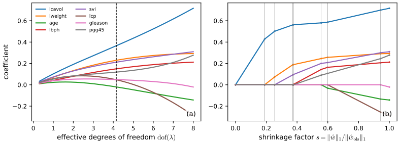
Table 11.1: lasso coefficients at the critical values of \(\lambda\)
| \(\lambda\) | lcavol | lweight | age | lbph | svi | lcp | gleason | pgg45 |
|---|---|---|---|---|---|---|---|---|
| 58.444 | 0.0000 | 0.0000 | 0.0000 | 0.0000 | 0.0000 | 0.0000 | 0.0000 | 0.0000 |
| 30.199 | 0.4279 | 0.0000 | 0.0000 | 0.0000 | 0.0000 | 0.0000 | 0.0000 | 0.0000 |
| 23.888 | 0.5015 | 0.0735 | 0.0000 | 0.0000 | 0.0000 | 0.0000 | 0.0000 | 0.0000 |
| 14.059 | 0.5610 | 0.1878 | 0.0000 | 0.0000 | 0.0930 | 0.0000 | 0.0000 | 0.0000 |
| 13.813 | 0.5622 | 0.1890 | 0.0000 | 0.0036 | 0.0963 | 0.0000 | 0.0000 | 0.0000 |
| 4.008 | 0.5797 | 0.2456 | 0.0000 | 0.1435 | 0.2003 | 0.0000 | 0.0000 | 0.0901 |
| 3.015 | 0.5864 | 0.2572 | -0.0321 | 0.1639 | 0.2082 | 0.0000 | 0.0000 | 0.1066 |
| 0.328 | 0.6994 | 0.2910 | -0.1337 | 0.2062 | 0.3003 | -0.2565 | 0.0000 | 0.2452 |
| 0.000 | 0.7164 | 0.2926 | -0.1425 | 0.2120 | 0.3096 | -0.2890 | -0.0209 | 0.2773 |
Reproduces Murphy (2022), Table 11.1 (the book's rows, without the \(\lambda\) column). Each row is a vertex of the piecewise linear path, computed by lars_lasso; the last row is least squares. The 67 training cases, predictors standardised, response centred, loss \(\frac12\|\bm y-\bm X\bm w\|^2\).
See also (companion): ESL 3.4.4, least angle regression and the LARS and lasso demo.
11.4.5 Comparison of least squares, lasso, ridge and subset selection
pp. 390–391 Take an orthonormal design, \(\bm X^\T\bm X=\bm I\). The criterion splits into one-dimensional problems and \[ \hat w^{\rm mle}_d=\bm x_{:,d}^\T\bm y,\qquad\hat w^{\rm ridge}_d=\frac{\hat w_d^{\rm mle}}{1+\lambda},\qquad\hat w^{\rm lasso}_d=\operatorname{sign}(\hat w_d^{\rm mle})(|\hat w_d^{\rm mle}|-\lambda)_+,\qquad\hat w^{\rm ss}_d=\hat w_d^{\rm mle}\,\mathbb I(\operatorname{rank}(|\hat w^{\rm mle}_d|)\le K), \tag{11.93–11.96} \] ridge scaling, lasso soft thresholding, subset selection hard thresholding.
Filling the gap 11.4e: the four estimators for an orthonormal design pp. 390–391, (11.91)–(11.96)
Derivation
With \(\bm X^\T\bm X=\bm I\), \[ \|\bm y-\bm X\bm w\|^2=\bm y^\T\bm y-2\bm w^\T\bm X^\T\bm y+\|\bm w\|^2=\mathrm{const}+\sum_d(w_d^2-2w_d\hat w_d^{\rm mle})=\mathrm{const}'+\sum_d(w_d-\hat w^{\rm mle}_d)^2 \] (11.91, 11.92), because \(\bm X^\T\bm y=\hat{\bm w}^{\rm mle}\). So with any penalty that separates over coordinates the problem decouples into \(\min_w\frac12(w-z)^2+\operatorname{pen}(w)\) with \(z=\hat w^{\rm mle}_d\).
Ridge (\(\frac\lambda2w^2\), the halved convention): \(w-z+\lambda w=0\Rightarrow w=z/(1+\lambda)\) (11.94). Lasso (\(\lambda|w|\)): the soft threshold \(\operatorname{sign}(z)(|z|-\lambda)_+\) by gap 11.4b with \(a=1\), \(c=z\) (11.95). Subset with penalty \(\lambda\mathbb I(w\ne0)\): hard threshold at \(\sqrt{2\lambda}\) as in gap 11.4b; choosing exactly \(K\) non-zero coordinates, the best subset keeps the \(K\) largest \(|z_d|\), because the residual sum of squares of a subset \(S\) is \(\|\bm y\|^2-\sum_{d\in S}z_d^2\) (orthonormality), minimised by taking the largest squares (11.96); ties are broken arbitrarily.
Bias and variance. For a true coefficient \(\beta\) and \(z\sim\mathcal N(\beta,\sigma^2)\): ridge multiplies by \(1/(1+\lambda)\), bias \(-\lambda\beta/(1+\lambda)\) and variance \(\sigma^2/(1+\lambda)^2\); the lasso shifts a large coefficient by \(-\lambda\operatorname{sign}\beta\) (bias \(\approx-\lambda\) once \(|\beta|\gg\lambda+\sigma\)); hard thresholding is nearly unbiased for large \(\beta\). That is why lasso coefficients of strong features are too small and why the debiasing step of Section 11.4.3 helps. \(\square\)
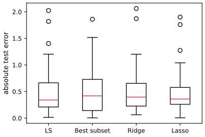
On the prostate data with 67 training and 30 test cases (the comparison of Hastie et al. 2009), Figure 11.11 lists the coefficients of the four methods at the tuning value chosen by 10-fold cross-validation with the one-standard-error rule (predictors standardised with all 97 cases), and Figure 11.12 the test errors. Subset selection is the sparsest, then the lasso; all four predict similarly.
Figure 11.11: coefficients and test error on the prostate data
| Term | OLS | Best subset | Ridge | Lasso |
|---|---|---|---|---|
| intercept | 2.465 | 2.477 | 2.459 | 2.467 |
| lcavol | 0.680 | 0.740 | 0.318 | 0.543 |
| lweight | 0.263 | 0.316 | 0.205 | 0.202 |
| age | -0.141 | 0.000 | -0.008 | 0.000 |
| lbph | 0.210 | 0.000 | 0.128 | 0.030 |
| svi | 0.305 | 0.000 | 0.188 | 0.113 |
| lcp | -0.288 | 0.000 | 0.060 | 0.000 |
| gleason | -0.021 | 0.000 | 0.050 | 0.000 |
| pgg45 | 0.267 | 0.000 | 0.110 | 0.028 |
| test error | 0.521 | 0.492 | 0.515 | 0.462 |
| std error | 0.179 | 0.143 | 0.179 | 0.159 |
Reproduces the layout of Murphy (2022), Figure 11.11 with my own cross-validation (10 folds, a fixed random split, one-standard-error rule; the chosen tuning values are 2 variables for the subset, \(\lambda=53.6\) for ridge and \(\lambda=11.3\) for the lasso in the halved convention). The test error is the mean squared error on the 30 test cases and its standard error. The numbers differ slightly from the book's because the cross-validation folds differ; the ordering (lasso lowest, subset and lasso sparse) agrees.
11.4.6 Variable selection consistency
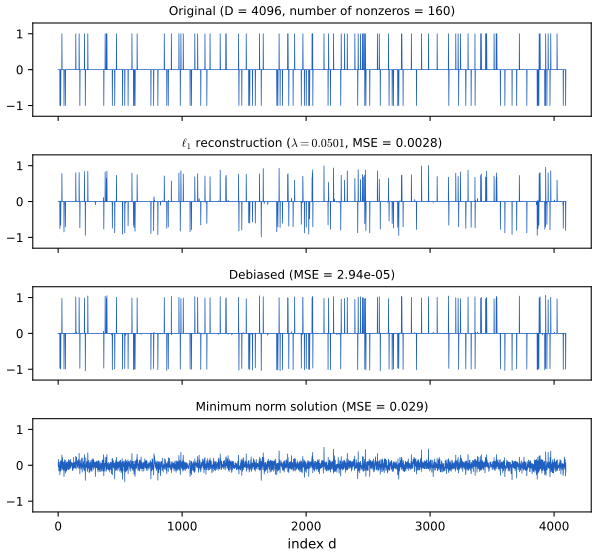
p. 392 An estimator that recovers the true support \(\{d:w^*_d\ne0\}\) with probability tending to one as \(N\to\infty\) is model selection consistent. Figure 11.13 generates a sparse signal \(\bm w^*\in\R^{4096}\) with 160 random \(\pm1\) spikes, a random design with \(N=1024\) and noise \(\sigma=0.01\). The lasso with \(\lambda=0.1\lambda_{\max}\) finds the support but the amplitudes are shrunk; the debiased fit recovers the signal; the minimum-norm least squares solution is dense. Cross-validation picks \(\lambda\) for prediction, which is generally not the value that recovers the true model (Meinshausen and Bühlmann 2006).
Filling the gap 11.4f: why the cross-validated \(\lambda\) does not recover the support, and what debiasing does pp. 389, 392
Derivation
Take an orthonormal design with \(s\) true non-zeros among \(D\) coordinates and noise level \(\sigma\); then \(z_d=\hat w_d^{\rm mle}\sim\mathcal N(w_d^*,\sigma^2)\) independently, and the lasso keeps coordinate \(d\) iff \(|z_d|>\lambda\) (gap 11.4e). For a null coordinate \(\Pr(\text{kept})=2(1-\Phi(\lambda/\sigma))\), so the expected number of false positives is \((D-s)\cdot2(1-\Phi(\lambda/\sigma))\). If \(\lambda/\sigma=c\) stays bounded as \(D\) grows, this tends to infinity: with a penalty tuned for prediction (which does not grow with \(D\), since the optimal amount of shrinkage depends on the signal-to-noise ratio, not on the number of nuisance coordinates) selection is inconsistent. To make it vanish we need \(c\) to grow like \(\sqrt{2\log D}\) (the universal threshold of Donoho and Johnstone): by the Mills ratio \(2(1-\Phi(c))\approx e^{-c^2/2}/(c\sqrt{\pi/2})\), so at \(c=\sqrt{2\log D}\) the expected number of false positives is about \(1/\sqrt{\pi\log D}\to0\). But such a large \(\lambda\) shrinks every retained coefficient by \(\lambda\), which hurts prediction. Prediction and selection therefore want different \(\lambda\), the point of the book's remark that cross-validation will typically include irrelevant variables (Meinshausen and Bühlmann 2006; for general designs a further "irrepresentable" condition is needed, Zhao and Yu 2006).
Debiasing. The two-stage estimator (lasso for the support \(\hat S\), then least squares on \(\hat S\)) satisfies, if \(\hat S\supseteq S^*\), \[ \hat{\bm w}_{\hat S}=(\bm X_{\hat S}^\T\bm X_{\hat S})^{-1}\bm X_{\hat S}^\T\bm y \], which is unbiased conditional on the support, with variance \(\sigma^2\operatorname{diag}(\bm X_{\hat S}^\T\bm X_{\hat S})^{-1}\), instead of the shrinkage bias of the lasso. In Figure 11.13 it reduces the MSE by a factor of about 100. \(\square\)
11.4.7 Group lasso
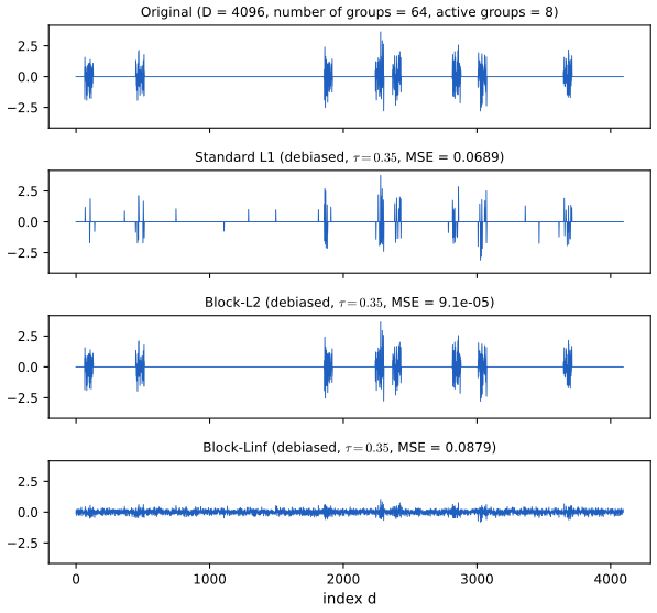
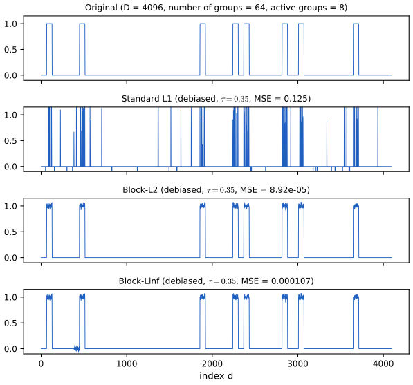
pp. 393–396 If each variable has a vector of weights (one-hot encoded categoricals, the outgoing weights of a feature in multinomial logistic regression, the incoming weights of a neuron, the weights of one feature across several tasks) we want all or none of a group \(\bm w_g\) to be non-zero: group sparsity. Partition \(\bm w=[\bm w_1,\dots,\bm w_G]\) and penalise the group norms, \[ \operatorname{PNLL}(\bm w)=\operatorname{NLL}(\bm w)+\lambda\sum_{g=1}^G\|\bm w_g\|_2,\qquad\|\bm w_g\|_2=\sqrt{\textstyle\sum_{d\in g}w_d^2} \tag{11.97} \] (group lasso, Yuan and Lin 2006). Squaring the group norms would give \(\sum_g\|\bm w_g\|_2^2=\|\bm w\|_2^2\), ridge (11.98); the square root penalises the radius of the group, and the only way to have small radius is to have all elements small. For a single group of two variables the derivative of \(\sqrt{w_1^2+w_2^2}\) is \(w_1/\sqrt{w_1^2+w_2^2}\) (11.99): if \(w_2\) is near zero the derivative tends to 1 and drives \(w_1\) to zero too, if \(w_2\) is large it tends to 0 and \(w_1\) is free. The variant with the infinity norm, \(\|\bm w_g\|_\infty=\max_{d\in g}|w_d|\) (11.100), also gives group sparsity and additionally tends to make the non-zero entries of a group equal in magnitude.
Filling the gap 11.4g: the proximal operators of the group norms pp. 394–396, (11.97)–(11.100)
Derivation
Block soft thresholding. The proximal operator of \(t\|\cdot\|_2\) is \[ \operatorname{prox}(\bm u)=\argmin_{\bm v}\frac12\|\bm v-\bm u\|^2+t\|\bm v\|_2 \]. The subdifferential of \(\|\cdot\|_2\) is \(\{\bm v/\|\bm v\|\}\) for \(\bm v\ne\bm 0\) and the unit ball at 0. If \(\bm v\ne\bm 0\) the optimality condition is \(\bm v-\bm u+t\bm v/\|\bm v\|=\bm 0\), i.e. \(\bm u=\bm v(1+t/\|\bm v\|)\): \(\bm v\) is parallel to \(\bm u\) with \(\|\bm v\|=\|\bm u\|-t\), possible iff \(\|\bm u\|>t\). If \(\|\bm u\|\le t\), then \(\bm v=\bm 0\) satisfies \(\bm 0\in-\bm u+t\,B\). Hence \(\operatorname{prox}(\bm u)=(1-t/\|\bm u\|)_+\bm u\): the whole group is set to zero when its norm is below \(t\), otherwise shrunk radially. Applied group by group it is the update of proximal gradient descent for (11.97); this is prox_block_l2. For groups of size 1 it reduces to soft thresholding.
The infinity norm. The function \(\|\cdot\|_\infty\) is the support function of the \(\ell_1\) unit ball, i.e. the conjugate of the indicator of \(\{\|\bm z\|_1\le1\}\). The Moreau decomposition \[ \bm u=\operatorname{prox}_{tf}(\bm u)+t\operatorname{prox}_{f^*/t}(\bm u/t) \] then gives \[ \operatorname{prox}_{t\|\cdot\|_\infty}(\bm u)=\bm u-\Pi_{\{\|\bm z\|_1\le t\}}(\bm u) \], the residual after projecting onto the \(\ell_1\) ball of radius \(t\) (computed by sorting in \(O(n\log n)\), Duchi et al. 2008); entries of largest magnitude are clipped down to a common level, which is why the \(\infty\)-norm equalises magnitudes within a group. This is prox_block_linf. \(\square\)
Figures 11.14 and 11.15 use a true signal with \(D=4096\) in 64 groups of 64, with 8 active groups, \(N=1024\) and noise variance \(10^{-4}\); the support is estimated by the standard lasso, the block-\(\ell_2\) and the block-\(\ell_\infty\) group lasso (with the same penalty \(\tau\)), then the non-zero values are re-fitted by least squares (debiased). In Figure 11.14 the non-zero values are standard normal; in 11.15 they are all equal to 1.
See also (companion): ESL 3.8.4, the grouped lasso.
11.4.8 Elastic net (ridge and lasso combined)
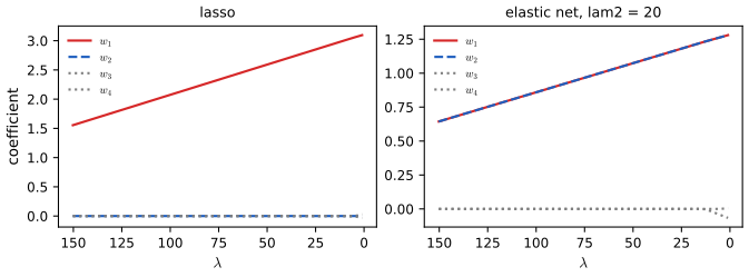
pp. 396–397 The elastic net (Zou and Hastie 2005) minimises \[ L(\bm w,\lambda_1,\lambda_2)=\|\bm y-\bm X\bm w\|^2+\lambda_2\|\bm w\|_2^2+\lambda_1\|\bm w\|_1. \tag{11.101} \] For \(\lambda_2>0\) the penalty is strictly convex, so the minimum is unique even if \(\bm X\) is rank deficient; it exhibits a grouping effect (coefficients of highly correlated variables tend to be equal; for identical features the estimates are equal, whereas the lasso may give one of them all the weight); and if \(D>N\) it can select more than \(N\) variables on its path.
Filling the gap 11.4h: uniqueness and the grouping effect of the elastic net, and Exercise 11.4 pp. 396–397, (11.101), Exercise 11.4
Derivation
Uniqueness. \(\|\bm y-\bm X\bm w\|^2\) is convex, \(\lambda_2\|\bm w\|^2\) is strongly convex for \(\lambda_2>0\), and \(\lambda_1\|\bm w\|_1\) is convex, so the sum is strongly convex and has exactly one minimiser, for any \(\bm X\).
Identical features. Suppose \(\bm x_{:,j}=\bm x_{:,k}\). The data-fit term depends on \((w_j,w_k)\) only through \(s=w_j+w_k\). For fixed \(s\), minimise \(\lambda_2(w_j^2+w_k^2)+\lambda_1(|w_j|+|w_k|)\): since \(w_j^2+w_k^2\ge s^2/2\) with equality iff \(w_j=w_k\) (strictly convex), and \(|w_j|+|w_k|\ge|s|\) with equality iff the two have the same sign (or one is zero), the equal split \(w_j=w_k=s/2\) minimises both terms at once. Any unequal split has a strictly larger \(\ell_2\) part, so by uniqueness \(\hat w_j=\hat w_k\). For the lasso (\(\lambda_2=0\)) every same-sign split of \(s\) gives the same penalty \(|s|\) and the same fit, so the minimiser is not unique and a solver may return \((s,0)\) (Figure 11.S1). More generally, strict convexity makes the coefficients of highly correlated features pull together.
Exercise 11.4 (reduction to a lasso). See the solution in Section 11.8.
11.4.9 Optimization algorithms
11.4.9.1 Coordinate descent
p. 397 Minimise over one coordinate at a time, \(w_j^*=\argmin_\eta L(\bm w+\eta\bm e_j)\) (11.102), cycling, sampling at random, or taking the steepest. For the lasso each one-dimensional problem is solved by soft thresholding (the shooting algorithm; the popular glmnet library generalises it to GLMs).
Algorithm 11.1: coordinate descent for the lasso (shooting algorithm)
- Initialise \(\bm w=(\bm X^\T\bm X+\lambda\bm I)^{-1}\bm X^\T\bm y\).
- Repeat until converged:
- for \(d=1,\dots,D\): \(a_d=\sum_nx_{nd}^2\); \(c_d=\sum_nx_{nd}(y_n-\bm w^\T\bm x_n+w_dx_{nd})\); \(w_d=\operatorname{SoftThreshold}(c_d/a_d,\lambda/a_d)\).
The update uses \(\bm x_n\) with the current residual \(y_n-\bm w^\T\bm x_n\), so it costs \(O(N)\) per coordinate if the residual is maintained. The code starts from \(\bm w=\bm 0\) or a warm start (the path from large to small \(\lambda\)).
11.4.9.2 Projected gradient descent
pp. 397–398 Split \(\bm w=\bm w^+-\bm w^-\) with \(\bm w^\pm\ge0\), \(\|\bm w\|_1\) replaced by \(\sum_d(w_d^++w_d^-)\): the smooth, constrained problem (11.103), a quadratic programme, solved by projected gradient descent (11.104) with the projection \(P_+\) onto the positive orthant, \(w\leftarrow\max(w,0)\).
11.4.9.3 Proximal gradient descent
p. 398 Using the proximal operator of \(\ell_1\), soft thresholding (Section 8.6.2), \[ \bm w_{t+1}=\operatorname{SoftThreshold}\big(\bm w_t-\eta_t\nabla\operatorname{NLL}(\bm w_t),\ \eta_t\lambda\big), \tag{11.105} \] the iterative soft thresholding algorithm (ISTA); with Nesterov acceleration it is FISTA (Beck and Teboulle 2009).
Filling the gap 11.4i: why the split-variable trick is exact, and the \(O(1/k)\) rate of ISTA pp. 397–398, (11.103)–(11.105)
Derivation
The split variable. For any \(\bm w\) the choice \(\bm w^+=\max(\bm w,0)\), \(\bm w^-=-\min(\bm w,0)\) has \(\sum_d(w^+_d+w^-_d)=\|\bm w\|_1\). For any other feasible split of the same \(\bm w\) (with \(w^\pm_d\ge0\), \(w_d^+-w_d^-=w_d\)) we have \(w^+_d+w^-_d=|w_d|+2\min(w^+_d,w^-_d)\ge|w_d|\), so minimising the linear penalty drives \(\min(w_d^+,w_d^-)\) to zero. The constrained problem (11.103) therefore has the same optimal value, and an optimal \(\bm w^+-\bm w^-\) solves the lasso.
Rate of ISTA. \(f(\bm w)=\frac12\|\bm y-\bm X\bm w\|^2\) has an \(L\)-Lipschitz gradient with \(L=\|\bm X\|_2^2=\sigma_{\max}(\bm X)^2\), and the step \(\eta=1/L\) is used. The ISTA update is the minimiser of the majorant \[ Q(\bm w;\bm z)=f(\bm z)+\nabla f(\bm z)^\T(\bm w-\bm z)+\frac L2\|\bm w-\bm z\|^2+\lambda\|\bm w\|_1 \], which satisfies \(Q\ge F\) (the descent lemma). Writing \(\bm w^+\) for the update from \(\bm z\), the strong convexity of \(Q\) (modulus \(L\)) and convexity of \(f\) give for every \(\bm u\): \[ F(\bm w^+)\le Q(\bm w^+;\bm z)\le Q(\bm u;\bm z)-\frac L2\|\bm u-\bm w^+\|^2\le F(\bm u)+\frac L2\|\bm u-\bm z\|^2-\frac L2\|\bm u-\bm w^+\|^2 \]. With \(\bm z=\bm w_k\), \(\bm u=\bm w_k\) shows \(F(\bm w_{k+1})\le F(\bm w_k)\); with \(\bm u=\bm w^\star\) and summing over \(i=0,\dots,k-1\), \[ \sum_{i=1}^k(F(\bm w_i)-F^\star)\le\frac L2\|\bm w_0-\bm w^\star\|^2 \]; monotonicity gives \(F(\bm w_k)-F^\star\le\frac{L\|\bm w_0-\bm w^\star\|^2}{2k}\). FISTA replaces \(\bm z=\bm w_k\) by an extrapolated point and improves the rate to \(O(1/k^2)\) (Beck and Teboulle 2009; I state this without proof). In the code, with the same number of iterations FISTA reaches a lower objective than ISTA and, run long enough, the coordinate descent solution (confirmed numerically). \(\square\)
11.4.9.4 LARS
pp. 398–399 Homotopy methods trace the whole path from \(\lambda_{\max}\) down, warm-starting each solution from the previous one. LARS (Efron et al. 2004) starts with the feature most correlated with \(\bm y\), decreases \(\lambda\) until a second feature has equally large correlation with the residual, and keeps the active features equiangular, solving analytically for the next critical \(\lambda\) (gap 11.4d). Variables may need to leave the active set; if removal is disallowed one obtains the (slightly different) LAR algorithm, close to forward selection and least squares boosting.
11.5 Regression splines *
p. 399 Polynomials are global approximations. Locality is easier to get with basis functions of local support; the notion is hard to define in high dimension, so this section is restricted to one-dimensional inputs, \(f(x;\bm\theta)=\sum_{i=1}^mw_iB_i(x)\) (11.106) with \(B_i\) the \(i\)th B-spline basis function.
11.5.1 B-spline basis functions
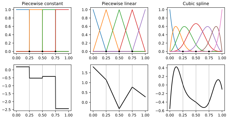
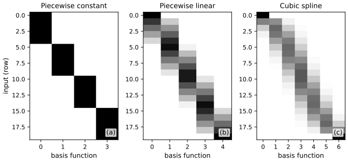
pp. 399–400 A spline of degree \(D\) is a piecewise polynomial of degree \(D\) on the intervals between knots \(t_1<\dots<t_m\), continuous with continuous derivatives of orders \(1,\dots,D-1\) at the knots; the cubic spline (\(D=3\)) has continuous value, slope and curvature. With \(K\) interior knots and degree \(D\) the B-spline basis has \(K+D+1\) functions. Figure 11.16 shows the bases of degree 0, 1 and 3 with knots 0.25, 0.5, 0.75 and (bottom row) random combinations; each basis function has local support: only \(D+1\) are non-zero at any \(x\). Figure 11.17 shows the design matrices on 20 equally spaced inputs: block diagonal (degree 0), banded (higher degree).
Filling the gap 11.5a: the Cox–de Boor recursion, partition of unity, local support, and the count \(K+D+1\) pp. 399–400
Derivation
The book skips how B-splines are computed. Let the knot sequence be \(\tau_1\le\dots\le\tau_{K+2D+2}\) (the interior knots, with the two boundary knots repeated \(D+1\) times each, so the basis is "clamped"). Degree 0: \(B_{i,0}(x)=1\) on \([\tau_i,\tau_{i+1})\), 0 elsewhere. For \(p\ge1\),
\[ B_{i,p}(x)=\frac{x-\tau_i}{\tau_{i+p}-\tau_i}B_{i,p-1}(x)+\frac{\tau_{i+p+1}-x}{\tau_{i+p+1}-\tau_{i+1}}B_{i+1,p-1}(x) \]
(a term with a zero denominator is dropped). The code bspline_basis implements exactly this and agrees with the SciPy design matrix (confirmed numerically).
Local support. By induction \(B_{i,p}\) vanishes outside \([\tau_i,\tau_{i+p+1})\), which contains \(p+1\) knot intervals; hence at any \(x\) at most \(p+1\) of the functions are non-zero (the "\(D+1\) active functions" of the book).
Partition of unity. \(\sum_iB_{i,p}(x)=1\) on \([\tau_{D+1},\tau_{K+D+2}]\). For \(p=0\) it holds because the intervals tile the domain. Assume it for \(p-1\); regrouping the recursion, \[ \sum_iB_{i,p}(x)=\sum_iB_{i,p-1}(x)\big[\frac{x-\tau_i}{\tau_{i+p}-\tau_i}+\frac{\tau_{i+p}-x}{\tau_{i+p}-\tau_i}\big]=\sum_iB_{i,p-1}(x)=1 \]. All \(B_{i,p}\ge0\) (a sum of non-negative terms on the support). So the basis consists of local bumps that average the weights \(w_i\): the fitted value at \(x\) is a convex combination of the \(D+1\) nearby weights, which also explains why a penalty on the weights is a sensible smoothness prior.
Dimension. Piecewise cubic polynomials on \(K+1\) intervals have \((K+1)(D+1)\) free coefficients; requiring continuity of the function and its first \(D-1\) derivatives at each of the \(K\) knots imposes \(KD\) linear conditions, leaving \((K+1)(D+1)-KD=K+D+1\) dimensions, which is the number of B-spline basis functions; they are a basis of this space (linearly independent by the local support and positivity of the functions on their supports; Schoenberg–Whitney conditions). The knots of Figure 11.16 give \(3+d+1\) functions: 4, 5 and 7 for \(d=0,1,3\), the column counts of Figure 11.17.
Smoothness. The recursion shows that \(B_{i,p}\) is continuous with continuous derivatives up to order \(p-1\) at simple knots, because \[ \frac{d}{dx}B_{i,p}=\frac p{\tau_{i+p}-\tau_i}B_{i,p-1}-\frac p{\tau_{i+p+1}-\tau_{i+1}}B_{i+1,p-1} \], each term being a spline of degree \(p-1\); induction gives \(C^{p-1}\). \(\square\)
11.5.2 Fitting a linear model using a spline basis
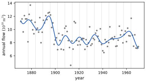
p. 401 Given the design matrix \(\bm B\) (rows \(B_i(x_n)\)), fit by least squares or, better, ridge regression. The book fits a cubic spline with 15 knots at quantiles of the inputs to the cherry blossom data; that series is not available offline, so Figure 11.18 uses a real stand-in with a similar irregular structure, the annual flow of the river Nile, 1871–1970 (100 points), fitted by ridge regression (\(\lambda=10^{-3}\)) on the 19 cubic B-splines with 15 quantile knots. More knots would fit better and eventually overfit; the number of knots (and \(\lambda\)) is chosen by cross-validation.
11.5.3 Smoothing splines
p. 401 Smoothing splines use \(N\) knots (one per data point), so the number of parameters grows with the data (a non-parametric model), and prevent overfitting by \(\ell_2\) regularisation; the method is closely related to Gaussian process regression (Chapter 17).
Filling the gap 11.5b: the smoothing spline is a natural cubic spline with knots at the data p. 401
Derivation
The book does not state the criterion; the usual one is \(\sum_n(y_n-f(x_n))^2+\lambda\int f''(t)^2\,dt\) over all twice-differentiable \(f\). Claim: the minimiser is a natural cubic spline with knots at the distinct \(x_n\) (cubic between knots, \(C^2\), and linear beyond the first and last knot). Proof: let \(g\) be any competitor and let \(s\) be the natural cubic spline interpolating \((x_n,g(x_n))\) (it exists and is unique, since there are \(N\) values and \(N\) degrees of freedom of natural splines). Put \(h=g-s\), so \(h(x_n)=0\). Integrating by parts over the intervals between knots, \[ \int_{x_1}^{x_N}s''h''\,dt=\big[s''h'\big]_{x_1}^{x_N}-\int s'''h'\,dt=-\sum_{j=1}^{N-1}s'''\big|_{(x_j,x_{j+1})}\,[h(x_{j+1})-h(x_j)]=0, \] because \(s''(x_1)=s''(x_N)=0\) (naturalness) and \(s'''\) is constant on each interval while \(h\) vanishes at the knots. Hence \(\int g''^2=\int s''^2+\int h''^2\ge\int s''^2\) (outside \([x_1,x_N]\) \(s''=0\) so \(s\) has no more roughness there than any \(g\)), while the data term is the same for \(g\) and \(s\). So the minimiser over \(g\) is a natural spline. Writing it as \(f=\sum_jN_j(x)\theta_j\) with \(N\) basis functions, the criterion becomes \(\|\bm y-\bm N\bm\theta\|^2+\lambda\bm\theta^\T\bm\Omega\bm\theta\) with \(\Omega_{jk}=\int N_j''N_k''\), minimised by \[ \hat{\bm\theta}=(\bm N^\T\bm N+\lambda\bm\Omega)^{-1}\bm N^\T\bm y \], a generalised ridge regression: a linear smoother whose degrees of freedom is \[ \operatorname{tr}[\bm N(\bm N^\T\bm N+\lambda\bm\Omega)^{-1}\bm N^\T] \] exactly as in gap 11.3b. The identical structure with a kernel in place of \(\bm\Omega\) is Gaussian process regression. \(\square\)
See also (companion): ESL 5.2, piecewise polynomials and splines, 5.4, smoothing splines, the regression splines demo and the smoothing spline demo; ISL 7.4.
11.5.4 Generalized additive models
pp. 401–402 A generalised additive model (GAM, Hastie and Tibshirani 1990) extends splines to \(D\) inputs by ignoring interactions: \(f(\bm x;\bm\theta)=\alpha+\sum_{d=1}^Df_d(x_d)\) (11.107), each \(f_d\) a regression or smoothing spline. It is fitted by backfitting: cycle over \(d\) and refit \(f_d\) to the partial residuals \(\bm y-\alpha-\sum_{k\ne d}f_k(\bm x_{:,k})\). With a link function the same idea applies to classification (Chapter 12).
Filling the gap 11.5c: backfitting is Gauss–Seidel on the normal equations pp. 401–402, (11.107)
Derivation
Each \(f_d\) is a linear smoother, \(\bm f_d=\bm S_d\bm r_d\) for its partial residual \(\bm r_d\), with \(\bm S_d\) the (ridge-like) smoother matrix of gap 11.5b; take \(\alpha=\bar y\) and centred \(\bm f_d\). The penalised additive criterion \[ \|\bm y-\alpha-\sum_d\bm f_d\|^2+\sum_d\lambda_d\bm f_d^\T\bm K_d\bm f_d \] has stationarity conditions \(\bm f_d=\bm S_d(\bm y-\alpha\bm 1-\sum_{k\ne d}\bm f_k)\) for \(d=1,\dots,D\), a block linear system \[ \begin{bmatrix}\bm I&\bm S_1&\cdots\\\bm S_2&\bm I&\cdots\\\vdots\end{bmatrix}\bm f=\begin{bmatrix}\bm S_1\bm y\\\bm S_2\bm y\\\vdots\end{bmatrix} \]. Backfitting solves it by block Gauss–Seidel: update each block in turn using the latest values of the others, i.e. \(\bm f_d\leftarrow\bm S_d(\bm y-\alpha\bm 1-\sum_{k\ne d}\bm f_k)\). For symmetric smoothers with eigenvalues in \([0,1]\) (smoothing splines) this is a coordinate descent on a convex quadratic and converges to a solution of the system (Buja, Hastie and Tibshirani 1989). It generalises the Gauss–Seidel iteration for OLS: with \(\bm S_d\) the projection onto the column \(\bm x_{:,d}\) it is exactly the coordinate update of gap 11.4b with \(\lambda=0\). Interactions are lost by construction. \(\square\)
See also (companion): the backfitting demo.
11.6 Robust linear regression *
p. 402 With Gaussian errors \(r_n=y_n-\bm w^\T\bm x_n\sim\mathcal N(0,\sigma^2)\), maximum likelihood is least squares, and because the squared error penalises large residuals quadratically a few outliers can pull the fit far away (Figure 11.19a). Replacing the Gaussian by a heavy-tailed distribution (Table 11.2) gives robustness: outliers then have much higher likelihood without moving the line.
Table 11.2: likelihoods, priors and posteriors for linear regression
| Likelihood | Prior | Posterior | Name | Section |
|---|---|---|---|---|
| Gaussian | uniform | point | least squares | 11.2.2 |
| Student | uniform | point | robust regression | 11.6.2 |
| Laplace | uniform | point | robust regression | 11.6.1 |
| Gaussian | Gaussian | point | ridge | 11.3 |
| Gaussian | Laplace | point | lasso | 11.4 |
| Gaussian | Gauss-Gamma | Gauss-Gamma | Bayesian linear regression | 11.7 |
Restated from Murphy (2022), Table 11.2. "Point" means the degenerate posterior at the MAP estimate.
11.6.1 Laplace likelihood
p. 402 With \[ p(y\given\bm x,\bm w,b)=\operatorname{Laplace}(y\given\bm w^\T\bm x,b)\propto\exp(-|y-\bm w^\T\bm x|/b) \] (11.108) the MLE minimises the sum of absolute residuals (least absolute deviations): robust because the penalty grows linearly, not quadratically.
11.6.1.1 Computing the MLE using linear programming
pp. 403–404 A linear programme minimises \(\bm c^\T\bm v\) subject to \(\bm A\bm v\le\bm b\) (11.109). With \(\bm v=(\bm w,e_1,\dots,e_N)\in\R^{D+N}\) (the \(e_i\) are the absolute residuals), \(\bm c=(\bm 0_D,\bm 1_N)\) and the two constraints per example \(e_i\ge\bm w^\T\bm x_i-y_i\) and \(e_i\ge-(\bm w^\T\bm x_i-y_i)\) (11.110, 11.111), i.e. \((\bm x_i,0,\dots,-1,\dots,0)^\T\bm v\le y_i\) and \((-\bm x_i,0,\dots,-1,\dots,0)^\T\bm v\le-y_i\) (11.112, 11.113), we obtain \(\bm A\in\R^{2N\times(N+D)}\) (11.114) and \(\bm b=(y_1,-y_1,\dots,y_N,-y_N)\) (11.115).
Filling the gap 11.6a: the LP is exactly least absolute deviations, and its solutions are lines through \(D\) points pp. 403–404, (11.109)–(11.115)
Derivation
Equivalence. For fixed \(\bm w\) the smallest feasible \(e_i\) is \[ \max(\bm w^\T\bm x_i-y_i,\,y_i-\bm w^\T\bm x_i)=|y_i-\bm w^\T\bm x_i| \], and the objective \(\sum e_i\) is increasing in each \(e_i\), so at the optimum all constraints are tight and the optimal value is \(\min_{\bm w}\sum_i|y_i-\bm w^\T\bm x_i|\) with the same \(\bm w\). (The book says the minimisation of \(\sum e_i\) "pushes down on" the constraints.) The LP is feasible and bounded below by 0, so an optimal solution exists.
Vertex solutions. A feasible LP with a bounded objective has an optimal vertex (when the feasible polyhedron has vertices, true here since \(\bm A\) has full column rank when the design does); at a vertex \(D+N\) of the \(2N\) constraints are tight, which for each \(i\) forces at most one of the two constraints of example \(i\) to be tight unless \(e_i=0\); the count shows that at least \(D\) examples have zero residual. So a least absolute deviation fit interpolates \(D\) of the data points (for a line, 2 points). The demo uses this: it finds the exact LAD line by checking all \(\binom N2\) lines through pairs of points and picking the one with the smallest sum of absolute residuals. \(\square\)
11.6.2 Student-t likelihood
p. 404 Putting the linear predictor in the location of a Student distribution (Zellner 1976), \[ p(y\given\bm x,\bm w,\sigma^2,\nu)=\mathcal T(y\given\bm w^\T\bm x,\sigma^2,\nu) \] (11.116), gives a robust model fitted by SGD or EM.
11.6.3 Huber loss
p. 404 The Huber loss \[ \ell_{\rm huber}(r,\delta)=\begin{cases}r^2/2&|r|\le\delta\\\delta|r|-\delta^2/2&|r|>\delta\end{cases} \tag{11.117} \] is quadratic for small errors and linear for large ones, and is everywhere differentiable, so smooth optimisers apply (much faster than the LP). The threshold \(\delta\) sets the degree of robustness and is set by hand or by cross-validation (Barron 2019 shows how to learn it).
Filling the gap 11.6b: the Student likelihood as a scale mixture, the EM algorithm, IRLS for Huber, and influence functions pp. 404, (11.116), (11.117)
Derivation
Scale mixture. The Student density is a Gaussian scale mixture: \[ \mathcal T(y\given\mu,\sigma^2,\nu)=\int_0^\infty\mathcal N(y\given\mu,\sigma^2/u)\,\operatorname{Ga}(u\given\frac\nu2,\frac\nu2)\,du \] (the integral of a Gaussian against a gamma over the precision multiplier \(u\) gives \(\propto(1+\frac{(y-\mu)^2}{\nu\sigma^2})^{-(\nu+1)/2}\)). Introduce one latent \(u_n\) per example.
EM. E-step: the posterior of \(u_n\) is \[ \operatorname{Ga}(\frac{\nu+1}2,\frac\nu2+\frac{r_n^2}{2\sigma^2}) \], with mean \(\bar u_n=\dfrac{\nu+1}{\nu+r_n^2/\sigma^2}\), \(r_n=y_n-\bm w^\T\bm x_n\). M-step: the expected complete-data log likelihood is, up to constants, \(-\frac1{2\sigma^2}\sum_n\bar u_nr_n^2-\frac N2\log\sigma^2\), so \(\bm w\leftarrow(\bm X^\T\bm U\bm X)^{-1}\bm X^\T\bm U\bm y\) with \(\bm U=\operatorname{diag}(\bar u_n)\) (weighted least squares, gap 11.2c) and \(\sigma^2\leftarrow\frac1N\sum_n\bar u_nr_n^2\). Points with large residuals receive small weights \(\bar u_n\approx(\nu+1)\sigma^2/r_n^2\): they are automatically down-weighted. EM increases the likelihood monotonically (student_em, started from the Laplace fit because the likelihood is not concave and has local optima).
Huber by IRLS. For a loss \(\rho(r)\) with \(\rho(r)/r\) non-increasing in \(|r|\), the quadratic \(\frac12u\,r^2+\mathrm{const}\) with \(u=\rho'(r_0)/r_0\) majorises \(\rho\) at \(r_0\); minimising the surrogate is weighted least squares with weights \(u_n=\psi(r_n)/r_n\), where \(\psi=\rho'\). For the Huber loss \(\psi(r)=\operatorname{clip}(r,-\delta,\delta)\), so \(u_n=\min(1,\delta/|r_n|)\): full weight to small residuals, weight \(\delta/|r_n|\) to large ones. Majorise–minimise decreases the (convex) objective each step and converges to the global minimum. The same recipe with \(\rho=|r|\) gives \(u_n=1/|r_n|\) (IRLS for the Laplace fit, singular at zero residuals).
Influence. The effect of one observation on the estimate is proportional to \(\psi\): for least squares \(\psi(r)=r\) (unbounded: one wild point can move the fit arbitrarily), for Laplace \(\psi=\operatorname{sign}(r)\) and Huber \(\operatorname{clip}(r,\pm\delta)\) (bounded), and for the Student likelihood \(\psi(r)=\frac{(\nu+1)r}{\nu\sigma^2+r^2}\), which is bounded and redescending: it goes back to 0 for \(|r|\to\infty\), so very distant outliers are ignored altogether (at the price of a non-convex objective). \(\square\)
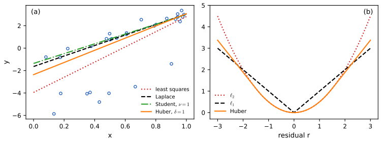
See also: the heavy-tails demo (Chapter 2).
11.6.4 RANSAC
pp. 404–405 In computer vision a common robust method is RANSAC (random sample consensus, Fischler and Bolles 1981): sample a small set of points, fit the model, find the points with small residuals under it (the inliers), refit on the inliers, repeat for many random starts and keep the best. A deterministic variant starts with all points as inliers, fits, removes points with large residuals and refits; despite making the problem non-convex it can be proved to converge rapidly under reasonable assumptions (Mukhoty et al. 2019; Suggala et al. 2019).
Filling the gap 11.6c: how many RANSAC trials are needed pp. 404–405
Derivation
Suppose a fraction \(\epsilon\) of the points are inliers and a minimal sample has \(m\) points (\(m=D\) for a linear model; 2 for a line). The probability that a random minimal sample is all inliers is \(\epsilon^m\) (to a good approximation when \(N\) is large; exactly \(\binom{N\epsilon}m/\binom Nm\)). Over \(T\) independent trials the probability that none is clean is \((1-\epsilon^m)^T\), so to have at least one clean sample with probability \(p\) we need \((1-\epsilon^m)^T\le1-p\), i.e.
\[ T\ge\frac{\log(1-p)}{\log(1-\epsilon^m)}. \]
For a line with 50% outliers (\(\epsilon=\frac12\), \(m=2\)) and \(p=0.99\): \(T\ge\log0.01/\log0.75=16.01\), so 17 trials; with \(m=7\) (a fundamental matrix in vision) it is 588. The count grows exponentially in \(m\), which is why RANSAC suits models with few parameters. A clean sample gives a fit near the truth, so the model with most inliers is good; the final refit on the inliers removes the noise of the minimal sample. In the code, ransac_line recovers the outliers of Figure 11.19's data (confirmed numerically). \(\square\)
11.7 Bayesian linear regression *
p. 405 We now compute the posterior \(p(\bm w\given\mathcal D)\) rather than a point estimate; for simplicity the noise variance \(\sigma^2\) is known (the general case is in the sequel to the book).
11.7.1 Priors
p. 405 Take a Gaussian prior \(p(\bm w)=\mathcal N(\bm w\given\breve{\bm w},\breve{\bm\Sigma})\) (11.118), a small generalisation of the ridge prior of Section 11.3.
11.7.2 Posteriors
p. 405 The likelihood is \[ p(\mathcal D\given\bm w,\sigma^2)=\mathcal N(\bm y\given\bm X\bm w,\sigma^2\bm I_N) \] (11.119) and by Bayes' rule for Gaussians (3.37) \[ p(\bm w\given\bm X,\bm y,\sigma^2)\propto\mathcal N(\bm w\given\breve{\bm w},\breve{\bm\Sigma})\,\mathcal N(\bm y\given\bm X\bm w,\sigma^2\bm I)=\mathcal N(\bm w\given\hat{\bm w},\hat{\bm\Sigma}), \tag{11.120} \] \[ \hat{\bm w}=\hat{\bm\Sigma}\Big(\breve{\bm\Sigma}^{-1}\breve{\bm w}+\frac1{\sigma^2}\bm X^\T\bm y\Big),\qquad\hat{\bm\Sigma}=\Big(\breve{\bm\Sigma}^{-1}+\frac1{\sigma^2}\bm X^\T\bm X\Big)^{-1}. \tag{11.121, 11.122} \] For \(\breve{\bm w}=\bm 0\), \(\breve{\bm\Sigma}=\tau^2\bm I\) the mean \(\hat{\bm w}=(\lambda\bm I+\bm X^\T\bm X)^{-1}\bm X^\T\bm y\), \(\lambda=\sigma^2/\tau^2\), is the ridge estimate (11.57).
Filling the gap 11.7a: the posterior by completing the square, and sequential updating p. 405, (11.120)–(11.122)
Derivation
Up to additive constants, \[ -2\log p(\bm w\given\mathcal D)=(\bm w-\breve{\bm w})^\T\breve{\bm\Sigma}^{-1}(\bm w-\breve{\bm w})+\sigma^{-2}(\bm y-\bm X\bm w)^\T(\bm y-\bm X\bm w)=\bm w^\T\hat{\bm\Sigma}^{-1}\bm w-2\bm w^\T\big(\breve{\bm\Sigma}^{-1}\breve{\bm w}+\sigma^{-2}\bm X^\T\bm y\big)+\mathrm{const} \], with \[ \hat{\bm\Sigma}^{-1}=\breve{\bm\Sigma}^{-1}+\sigma^{-2}\bm X^\T\bm X \] (11.122). Completing the square, \[ =(\bm w-\hat{\bm w})^\T\hat{\bm\Sigma}^{-1}(\bm w-\hat{\bm w})+\mathrm{const} \] with \[ \hat{\bm w}=\hat{\bm\Sigma}(\breve{\bm\Sigma}^{-1}\breve{\bm w}+\sigma^{-2}\bm X^\T\bm y) \] (11.121). So the posterior is Gaussian; its precision is the prior precision plus the data precision \(\sigma^{-2}\bm X^\T\bm X\), and the mean is the precision-weighted combination of the prior mean and the least squares information. The posterior is also the MAP, and the covariance does not depend on \(\bm y\).
Sequential updating. Because the data are conditionally independent given \(\bm w\), the posterior after \(n\) points is the prior for point \(n+1\): precision \[ \hat{\bm\Sigma}_{n+1}^{-1}=\hat{\bm\Sigma}_n^{-1}+\sigma^{-2}\bm x_{n+1}\bm x_{n+1}^\T \] (a rank-one update, so \(\hat{\bm\Sigma}_{n+1}\) follows from the Sherman–Morrison formula in \(O(D^2)\)). This is the mechanism of Figure 11.20, and it is the recursive estimator of Section 11.2.3.4 with a prior; the same numbers come out of a batch update on all \(N\) points (confirmed numerically). \(\square\)
11.7.3 Example
p. 406 For \(f(x;\bm w)=w_0+w_1x\) with true parameters \(w_0=-0.3\), \(w_1=0.5\), Figure 11.20 plots, as the number of data points grows, the likelihood of the latest point, the posterior, and samples from the posterior predictive. With \(N=0\) the posterior is the prior; for \(N=1\) it is constrained to a ridge (many slopes and intercepts pass near one point); at \(N=2\) it is narrow; at \(N=100\) it is essentially a point at \(\bm w^*\): the Bayesian estimate is consistent and the posterior uncertainty shrinks.
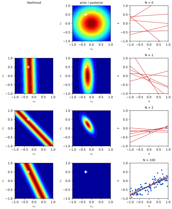
See also (companion): Bishop 3.3.1, the parameter distribution and the Bayesian regression demo.
11.7.4 Computing the posterior predictive
pp. 406–407 The posterior predictive at a test input \(\bm x\) is Gaussian (using (3.38)): \[ p(y\given\bm x,\mathcal D,\sigma^2)=\int\mathcal N(y\given\bm x^\T\bm w,\sigma^2)\,\mathcal N(\bm w\given\hat{\bm\mu},\hat{\bm\Sigma})\,d\bm w=\mathcal N\big(y\given\hat{\bm\mu}^\T\bm x,\ \hat\sigma^2(\bm x)\big),\qquad\hat\sigma^2(\bm x)=\sigma^2+\bm x^\T\hat{\bm\Sigma}\bm x. \tag{11.123–11.124} \] The variance has the noise \(\sigma^2\) plus the parameter uncertainty propagated through \(\bm x\), which grows away from the training inputs (Figure 11.21b: error bars widen), important for example in active learning. With a point estimate \(\hat{\bm w}\) one uses the plug-in approximation \(p(y\given\bm x,\hat{\bm w},\sigma^2)\) (11.125): constant variance, independent of the data (11.21a), and a single function when sampling (11.21c), whereas sampling from the posterior gives a range of functions (11.21d).
Filling the gap 11.7b: derivation of the predictive (11.124), its variance, and why it grows away from the data pp. 406–407, (11.123)–(11.125)
Derivation
Write \(y=\bm x^\T\bm w+\varepsilon\) with \(\bm w\sim\mathcal N(\hat{\bm\mu},\hat{\bm\Sigma})\) and \(\varepsilon\sim\mathcal N(0,\sigma^2)\) independent. Then \(y\) is a linear function of jointly Gaussian variables, hence Gaussian, with mean \(\bm x^\T\hat{\bm\mu}\) and variance \(\bm x^\T\hat{\bm\Sigma}\bm x+\sigma^2\) (the covariance between \(\bm x^\T\bm w\) and \(\varepsilon\) is 0). This is (11.124) and avoids evaluating the integral (11.123) directly; it is also a special case of the marginal of a linear Gaussian system, Equation (3.38). Equivalently, the predictive mean is the posterior mean of the function and the variance is its posterior variance plus the noise.
Explicit form for a straight line under a flat prior. Then \(\hat{\bm\Sigma}=\sigma^2(\bm X^\T\bm X)^{-1}\) and for \(\bm x=(1,x)^\T\), \[ \bm x^\T(\bm X^\T\bm X)^{-1}\bm x=\frac1N+\frac{(x-\bar x)^2}{\sum_n(x_n-\bar x)^2} \] (centre the inputs: \(\bm X^\T\bm X\) becomes diagonal, gap 11.7c). So \[ \hat\sigma^2(x)=\sigma^2\Big[1+\frac1N+\frac{(x-\bar x)^2}{\sum_n(x_n-\bar x)^2}\Big]: \] a parabola with its minimum at \(\bar x\), at least \(\sigma^2(1+1/N)\), and growing quadratically with the distance from the centre of the training inputs. As \(N\to\infty\) it tends to \(\sigma^2\) everywhere the inputs have mass. The plug-in predictive has the constant variance \(\sigma^2\) (or \(\hat\sigma^2_{\rm mle}\)) and so under-states the uncertainty, most severely at the edges. \(\square\)
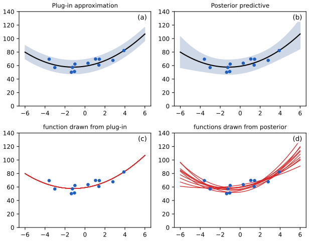
11.7.5 The advantage of centering
pp. 408–409 The posterior of \((w_0,w_1)\) in Figure 11.20 is an elongated diagonal ellipse: every data point induces a likelihood that is a ridge of lines through that point, and the lines with high likelihood for all points pass through the data mean \((\bar x,\bar y)\); increasing the slope requires decreasing the intercept, like a wheel pivoting about a point. Centring the inputs, \(x'_n=x_n-\bar x\), lets the lines pivot about the origin and removes the posterior correlation (Figure 11.22). Parameters in the original coordinates follow from \(y'=w_0'+w_1'(x-\bar x)=(w_0'-w_1'\bar x)+w_1'x\), i.e. \(w_0=w_0'-w_1'\bar x\), \(w_1=w_1'\) (11.126). (One may also divide by the standard deviation of \(x\).)
Filling the gap 11.7c: the posterior correlation of intercept and slope, and why centring removes it pp. 408–409, (11.126)
Derivation
Under a flat prior (or a weak one) the posterior covariance is \(\sigma^2(\bm X^\T\bm X)^{-1}\). For the design \(\bm X=[\bm 1,\bm x]\), \[ \bm X^\T\bm X=\begin{bmatrix}N&N\bar x\\N\bar x&\sum x_n^2\end{bmatrix} \] and its inverse is \[ \frac1{N\sum(x_n-\bar x)^2}\begin{bmatrix}\sum x_n^2&-N\bar x\\-N\bar x&N\end{bmatrix} \]. So \[ \operatorname{corr}(w_0,w_1)=\frac{-N\bar x}{\sqrt{\sum x_n^2\cdot N}}=-\frac{\bar x}{\sqrt{\overline{x^2}}}=-\frac{\bar x}{\sqrt{\bar x^2+s_x^2}},\qquad s_x^2=\frac1N\sum(x_n-\bar x)^2. \] It is close to \(-1\) when the mean of the inputs is large compared with their spread, and exactly 0 when \(\bar x=0\) (centred inputs: \(\bm X^\T\bm X\) is diagonal). In the example of Figure 11.22 (inputs in \([4,10]\)) it is \(-0.975\) before centring and \(0.04\) after (the sampled value, which is 0 up to sampling error). The correlation is a coordinate artefact: centring is the change of basis that diagonalises the design, it does not change the fit or the predictions, and the back-transformation (11.126) recovers the original parameters; but an elongated, tilted posterior is hard for a sampler or a mean-field approximation to explore, so centring (and scaling) helps computation. With an informative prior the same conclusion holds approximately. \(\square\)
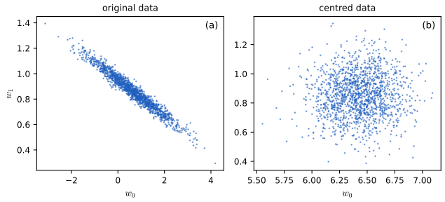
11.7.6 Dealing with multicollinearity
pp. 409–410 When inputs are highly correlated, including all of them does not hurt prediction (with regularisation) but it makes the coefficients hard to interpret. The toy example: heights \(h_i\sim\mathcal N(10,2)\) (the book writes variance as the second argument; here the standard deviation is 2), a leg fraction \(\rho_i\sim\operatorname{Unif}(0.4,0.5)\), and left and right leg lengths \(l_i,r_i\sim\mathcal N(\rho_ih_i,0.02)\), both noisy measurements of the same quantity. Regress \(h\) on \((l,r)\), \[ p(h\given l,r)=\mathcal N(h\given\alpha+\beta_ll+\beta_rr,\sigma^2) \] with vague priors \(\alpha,\beta_l,\beta_r\sim\mathcal N(0,100)\) and \(\sigma\sim\operatorname{Expon}(1)\). One expects \(\beta_l\approx\beta_r\approx h/l\approx2.2\), but the posterior marginals (Figure 11.23) show a large coefficient on one leg and a small or negative one on the other; and which leg depends on the sample. The joint posterior (Figure 11.24a) is a thin line: the two are nearly perfectly negatively correlated, so each is individually unidentified, but their sum is well determined (11.24b), centred near 2.2.
Filling the gap 11.7d: why only the sum of two collinear coefficients is determined pp. 409–410, Figures 11.23–11.24
Derivation
Let \(\bm X=[\bm l,\bm r]\) (ignore the intercept) with \(\bm l\approx\bm r\). The Gram matrix is, in the basis \(\bm u_+=(1,1)/\sqrt2\), \(\bm u_-=(1,-1)/\sqrt2\), approximately diagonal with eigenvalues \(\lambda_+=\|\bm l+\bm r\|^2/2\approx2\|\bm l\|^2\) (huge) and \(\lambda_-=\|\bm l-\bm r\|^2/2\) (tiny, because \(\bm l-\bm r\) is just measurement noise, standard deviation \(0.02\sqrt2\)). Under a vague prior the posterior covariance is \(\approx\sigma^2(\bm X^\T\bm X)^{-1}\), with variance \(\sigma^2/\lambda_+\) along \(\bm u_+\) and \(\sigma^2/\lambda_-\) along \(\bm u_-\): \(\operatorname{var}(\beta_l+\beta_r)=2\sigma^2/\lambda_+\) is small (determined by the data: the standard deviation of \(\beta_l+\beta_r\) is 0.07 in our run) while \(\operatorname{var}(\beta_l-\beta_r)=2\sigma^2/\lambda_-\) is enormous, limited only by the prior (standard deviation 4.3 in our run). The ratio of the two variances is \(\lambda_+/\lambda_-\), the condition number of the Gram matrix: \(1.2\times10^5\) here (eigenvalues 3769 and 0.032). The marginal of \(\beta_l\) is then wide, with an unstable sign, while the sum is stable. The sign is decided by sampling noise in the tiny direction \(\bm l-\bm r\), which is why a rerun may favour the other leg. The lesson: a coefficient measures the value of a feature given all the others (partial regression, gap 11.2d), so for collinear features individual coefficients do not carry meaning, only well-determined combinations do. (In the figures the exact posterior is used: the weights \((\alpha,\beta_l,\beta_r)\) are integrated out analytically and \(\sigma\) is drawn from its one-dimensional posterior on a grid, so the draws are exact; the book uses MCMC.) \(\square\)
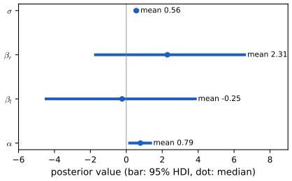
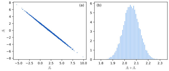
11.7.7 Automatic relevancy determination (ARD) *
pp. 410–411 With known noise and prior \(w_j\sim\mathcal N(0,1/\alpha_j)\), estimate the precisions by maximising the marginal likelihood (empirical Bayes), \(\hat{\bm\alpha}=\argmax_{\bm\alpha}p(\bm y\given\bm X,\bm\alpha)\) (11.127), \[ p(\bm y\given\bm X,\bm\alpha)=\int p(\bm y\given\bm X\bm w,\sigma^2)\,p(\bm w\given\bm 0,\operatorname{diag}(\bm\alpha)^{-1})\,d\bm w \] (11.128); then the MAP estimate \[ \hat{\bm w}=\argmax_{\bm w}\mathcal N(\bm w\given\bm 0,\hat{\bm\alpha}^{-1}) \] (11.129, as the book writes it; it is the posterior mean given \(\hat{\bm\alpha}\)) is sparse, although the prior is Gaussian: sparse Bayesian learning (Tipping 2001) or ARD (MacKay 1995; Neal 1996).
Filling the gap 11.7e: why maximising the evidence switches features off (a one-coefficient proof) pp. 410–411, (11.127)–(11.129)
Derivation
The book leaves the reason to the sequel; the mechanism is visible with one coefficient. Let \(\bm y=\bm xw+\bm\varepsilon\) with \(\|\bm x\|=1\), \(\bm\varepsilon\sim\mathcal N(\bm 0,\sigma^2\bm I)\), \(w\sim\mathcal N(0,\gamma)\), \(\gamma=1/\alpha\), and \(z=\bm x^\T\bm y\). Integrating \(w\) out, \(\bm y\sim\mathcal N(\bm 0,\bm C)\) with \(\bm C=\sigma^2\bm I+\gamma\bm x\bm x^\T\), \(\det\bm C=\sigma^{2(N-1)}(\sigma^2+\gamma)\) and \[ \bm y^\T\bm C^{-1}\bm y=\sigma^{-2}(\|\bm y\|^2-z^2)+z^2/(\sigma^2+\gamma) \]. Hence \[ -2\log p(\bm y\given\gamma)=\log(\sigma^2+\gamma)+\frac{z^2}{\sigma^2+\gamma}+\mathrm{const}. \] Its derivative in \(\gamma\) is \[ \frac1{\sigma^2+\gamma}-\frac{z^2}{(\sigma^2+\gamma)^2}=\frac{\sigma^2+\gamma-z^2}{(\sigma^2+\gamma)^2} \], which is zero at \(\gamma=z^2-\sigma^2\) and is positive for all \(\gamma\ge0\) when \(z^2\le\sigma^2\). So \[ \hat\gamma=\max(z^2-\sigma^2,0),\qquad\hat\alpha=\frac1{(z^2-\sigma^2)_+}. \] If the feature explains less than the noise level (\(z^2\le\sigma^2\)) the evidence is maximised at \(\gamma=0\), that is \(\alpha=\infty\): the prior pins \(w\) to exactly 0, and the feature is removed. If \(z^2>\sigma^2\) the weight has the posterior mean \(\frac{\hat\gamma}{\hat\gamma+\sigma^2}z=(1-\sigma^2/z^2)z\), a "garrote" shrinkage. This gives a sparse estimate from a Gaussian prior because the prior scale is itself estimated: marginally the prior over \(w\) is a scale mixture, which is heavier-tailed and peaked at zero, like the Laplace prior. (The closed form is confirmed numerically; for several correlated features the evidence is optimised by iterations, e.g. EM or fixed point updates.) \(\square\)
See also (companion): Bishop 3.5, the evidence approximation and the relevance vector machine demo.
11.8 Exercises
All six exercises of Chapter 11 (Murphy, 2022, pp. 411–413), restated in my own words, with complete solutions (hidden). Dagger marks the book's own flag for solutions available in its solution material; here every solution is worked independently.
Exercise 11.1 (multi-output linear regression). A two-dimensional response \(\bm y_i\in\R^2\) is observed for a binary input \(x_i\in\{0,1\}\): for \(x=0\) the three responses are \((-1,-1)^\T\), \((-1,-2)^\T\), \((-2,-1)^\T\); for \(x=1\) they are \((1,1)^\T\), \((1,2)^\T\), \((2,1)^\T\). Embed \(x\) as \(\bm\phi(0)=(1,0)^\T\), \(\bm\phi(1)=(0,1)^\T\) and fit \(\hat{\bm y}=\bm W^\T\bm\phi(x)\) with \(\bm W\in\R^{2\times2}\). Find the MLE of \(\bm W\).
Solution
The design matrix \(\bm\Phi\) has rows \(\bm\phi(x_i)\): three rows \((1,0)\) then three rows \((0,1)\), so \(\bm\Phi^\T\bm\Phi=3\bm I_2\) and \(\bm\Phi^\T\bm Y\) has as its two rows the sums of the responses in each group: \((-4,-4)\) and \((4,4)\). The multivariate MLE (11.2) solves each output column separately, \[ \hat{\bm W}=(\bm\Phi^\T\bm\Phi)^{-1}\bm\Phi^\T\bm Y=\frac13\begin{bmatrix}-4&-4\\4&4\end{bmatrix} \], that is \[ \hat{\bm W}=\begin{bmatrix}-4/3&-4/3\\4/3&4/3\end{bmatrix}. \] Each row is the mean response of the group (with one-hot features, regression is the group mean); \(\hat{\bm y}(0)=\bm W^\T(1,0)^\T=(-4/3,-4/3)^\T\) and \(\hat{\bm y}(1)=(4/3,4/3)^\T\). Confirmed with
np.linalg.lstsq. \(\square\)Exercise 11.2 (centring and ridge regression). Assume \(\bar{\bm x}=\bm 0\) (centred inputs). Show that the minimiser of \[ J(\bm w,w_0)=(\bm y-\bm X\bm w-w_0\bm 1)^\T(\bm y-\bm X\bm w-w_0\bm 1)+\lambda\bm w^\T\bm w \] is \(\hat w_0=\bar y\) and \(\hat{\bm w}=(\bm X^\T\bm X+\lambda\bm I)^{-1}\bm X^\T\bm y\).
Solution
\(J\) is strictly convex in \((\bm w,w_0)\) for \(\lambda>0\) (the Hessian in \(\bm w\) is \(2(\bm X^\T\bm X+\lambda\bm I)\succ0\), the Hessian in \(w_0\) is \(2N>0\), and the cross-block is \(2\bm X^\T\bm 1=2N\bar{\bm x}=\bm 0\)), so stationarity characterises the minimiser. \[ \partial J/\partial w_0=-2\bm 1^\T(\bm y-\bm X\bm w-w_0\bm 1)=-2(N\bar y-N\bar{\bm x}^\T\bm w-Nw_0)=0 \] gives \(w_0=\bar y-\bar{\bm x}^\T\bm w=\bar y\) because \(\bar{\bm x}=\bm 0\) (the offset is not penalised, so this holds for every \(\lambda\)). \[ \partial J/\partial\bm w=-2\bm X^\T(\bm y-\bm X\bm w-w_0\bm 1)+2\lambda\bm w=0 \]; since \(\bm X^\T\bm 1=N\bar{\bm x}=\bm 0\) the \(w_0\) term drops out, leaving \((\bm X^\T\bm X+\lambda\bm I)\bm w=\bm X^\T\bm y\), i.e. (11.134). If the offset were penalised (\(w_0\) in the ridge term) the optimum would be \(\bar y\,N/(N+\lambda)\), biasing the baseline towards 0; this is why it is excluded. For uncentred inputs the same solution is obtained by centring \(\bm X\) and \(\bm y\), fitting \(\bm w\), and \(w_0=\bar y-\bar{\bm x}^\T\bm w\) (gap 11.2d). \(\square\)
Exercise 11.3 (partial derivative of the RSS \(\dagger\)). Let \(\operatorname{RSS}(\bm w)=\|\bm X\bm w-\bm y\|_2^2\). (a) Show \(\frac\partial{\partial w_k}\operatorname{RSS}=a_kw_k-c_k\) with \(a_k=2\|\bm x_{:,k}\|^2\), \(c_k=2\bm x_{:,k}^\T\bm r_k\), \(\bm r_k=\bm y-\bm X_{:,-k}\bm w_{-k}\). (b) If the derivative is zero then \(\hat w_k=\bm x_{:,k}^\T\bm r_k/\|\bm x_{:,k}\|^2\).
Solution
(a) Partition the weights into \(w_k\) and \(\bm w_{-k}\): \(\bm X\bm w=\bm x_{:,k}w_k+\bm X_{:,-k}\bm w_{-k}\), so \(\bm X\bm w-\bm y=\bm x_{:,k}w_k-\bm r_k\). Then \[ \operatorname{RSS}=\|\bm x_{:,k}w_k-\bm r_k\|^2=w_k^2\|\bm x_{:,k}\|^2-2w_k\bm x_{:,k}^\T\bm r_k+\|\bm r_k\|^2 \], where \(\bm r_k\) does not depend on \(w_k\). Differentiating, \(2w_k\|\bm x_{:,k}\|^2-2\bm x_{:,k}^\T\bm r_k=a_kw_k-c_k\). Writing out coordinates, \(\|\bm x_{:,k}\|^2=\sum_ix_{ik}^2\) and \(\bm x_{:,k}^\T\bm r_k=\sum_ix_{ik}(y_i-\bm w_{-k}^\T\bm x_{i,-k})\).
(b) Setting \(a_kw_k=c_k\) gives \(w_k=c_k/a_k=\bm x_{:,k}^\T\bm r_k/\|\bm x_{:,k}\|^2\) (the factors 2 cancel). This is the coefficient of the orthogonal projection of \(\bm r_k\) onto \(\bm x_{:,k}\) (11.17): adding features one at a time, the optimal weight of the new feature is the projection coefficient of the current residual; this is the coordinate update of Algorithm 11.1 for \(\lambda=0\). With the halved loss of (11.6) the same computation gives \(a_k=\|\bm x_{:,k}\|^2\), \(c_k=\bm x_{:,k}^\T\bm r_k\): this is the version that agrees with (11.81)–(11.83). \(\square\)
Exercise 11.4 (reducing the elastic net to the lasso). Define \[ J_1(\bm w)=\|\bm y-\bm X\bm w\|^2+\lambda_2\|\bm w\|_2^2+\lambda_1\|\bm w\|_1 \] and \[ J_2(\bm w)=\|\tilde{\bm y}-\tilde{\bm X}\bm w\|^2+c\lambda_1\|\bm w\|_1 \] with \(c=(1+\lambda_2)^{-1/2}\), \[ \tilde{\bm X}=c\begin{bmatrix}\bm X\\\sqrt{\lambda_2}\bm I_d\end{bmatrix} \], \(\tilde{\bm y}=\begin{bmatrix}\bm y\\\bm 0_{d\times1}\end{bmatrix}\). Show \(J_1(c\bm w)=J_2(\bm w)\), hence \(\argmin J_1=c\,\argmin J_2\).
Solution
Expand \(J_2\): \[ \tilde{\bm y}-\tilde{\bm X}\bm w=\begin{bmatrix}\bm y-c\bm X\bm w\\-c\sqrt{\lambda_2}\bm w\end{bmatrix} \], so \[ \|\tilde{\bm y}-\tilde{\bm X}\bm w\|^2=\|\bm y-c\bm X\bm w\|^2+c^2\lambda_2\|\bm w\|_2^2 \]. Hence \[ J_2(\bm w)=\|\bm y-\bm X(c\bm w)\|^2+\lambda_2\|c\bm w\|_2^2+\lambda_1\|c\bm w\|_1 \], because \(c^2\|\bm w\|^2=\|c\bm w\|^2\) and \(c\lambda_1\|\bm w\|_1=\lambda_1\|c\bm w\|_1\) (\(c>0\)). That is \(J_2(\bm w)=J_1(c\bm w)\). Since \(\bm w\mapsto c\bm w\) is a bijection, \(\bm w^\star\) minimises \(J_2\) iff \(c\bm w^\star\) minimises \(J_1\): \(\argmin J_1=c\,\argmin J_2\). So an elastic net problem is solved by augmenting the data with \(d\) rows (a ridge-like prior) and rescaling, then running any lasso solver (the same trick as the virtual data of gap 11.3a), and multiplying by \(c\); the factor \(c=1/\sqrt{1+\lambda_2}\) is the "naive elastic net" correction that undoes the double shrinkage. In the code, the elastic net by coordinate descent and the lasso solver on the augmented data agree to \(10^{-6}\) (confirmed numerically). \(\square\)
Exercise 11.5 (shrinkage in linear regression \(\dagger\)). For an orthonormal design (\(\|\bm x_{:,k}\|^2=1\), \(\bm x_{:,k}^\T\bm x_{:,j}=0\)), each \(\hat w_k\) can be estimated separately; the book's figure plots \(\hat w_k\) against \(c_k=2\bm y^\T\bm x_{:,k}\) for OLS, ridge with parameter \(\lambda_2\) and lasso with parameter \(\lambda_1\), three lines (solid, dotted, dashed) whose labels are lost. (a) Which line is which? (b) What is \(\lambda_1\)? (c) What is \(\lambda_2\)? (The reference "Figure 10.15b" in the exercise is a stale cross-reference; the figure is not part of the chapter text, so the answer is given in terms of what the three curves look like.)
Solution
With \(\|\bm y-\bm X\bm w\|^2+\lambda_2\|\bm w\|^2+\lambda_1\|\bm w\|_1\) and an orthonormal design, \(\operatorname{OLS}\) gives \(\hat w_k=\bm x_{:,k}^\T\bm y=c_k/2\): a line of slope \(\frac12\) through the origin. Ridge (\(\lambda_1=0\)) gives \(\hat w_k=\frac{c_k/2}{1+\lambda_2}\): a line through the origin with the smaller slope \(\frac1{2(1+\lambda_2)}\). The lasso (\(\lambda_2=0\), unhalved loss, gap 11.4b: soft threshold at \(\lambda_1/2\) in the variable \(\bm x_{:,k}^\T\bm y=c_k/2\)) gives \(\hat w_k=\operatorname{sign}(c_k)(|c_k|-\lambda_1)_+/2\): exactly zero for \(|c_k|\le\lambda_1\), then a line of slope \(\frac12\) shifted by \(\lambda_1/2\). (a) So: the line of slope \(\frac12\) that passes through the origin is OLS; the line through the origin with a smaller slope is ridge; the curve with a flat zero segment and then parallel to OLS but displaced is the lasso. (b) \(\lambda_1\) is the half-width of the flat segment on the \(c_k\) axis (the abscissa where the lasso leaves zero); equivalently the horizontal distance between the lasso curve and the OLS line far from the origin. (c) \[ \lambda_2=\frac{\text{slope}_{\rm OLS}}{\text{slope}_{\rm ridge}}-1=\frac{1/2}{s_{\rm ridge}}-1 \]. For instance, a ridge slope of \(\frac14\) means \(\lambda_2=1\). The mapping of the figure's three line styles to the three methods follows from these shapes. The shapes are what the lines of Figure 11.9a and gap 11.4e show; I checked the three closed forms against numerical minimisation of the unhalved objectives (confirmed numerically; the unhalved lasso threshold is \(\lambda_1/2\) in the least-squares coordinate, the point of the factor-2 remark in the notes on the book). \(\square\)
Exercise 11.6 (EM for a mixture of linear regression experts). Derive the EM equations for fitting a mixture of \(K\) linear regression experts.
Solution
Model. A latent \(z_n\in\{1,\dots,K\}\) chooses the expert: \(p(z_n=k\given\bm x_n)=\pi_k(\bm x_n)\) and \[ p(y_n\given\bm x_n,z_n=k)=\mathcal N(y_n\given\bm w_k^\T\bm x_n,\sigma_k^2) \]. (The simple mixture has constant mixing weights \(\pi_k\); the "experts" version has a gating function, e.g. \(\pi_k(\bm x)=\operatorname{softmax}_k(\bm v_k^\T\bm x)\).) The log likelihood \[ \sum_n\log\sum_k\pi_k(\bm x_n)\mathcal N(y_n\given\bm w_k^\T\bm x_n,\sigma_k^2) \] has the sum inside the logarithm, so we maximise it by EM.
E-step. With current parameters, the responsibilities are the posterior of \(z_n\): \[ r_{nk}=p(z_n=k\given\bm x_n,y_n)=\frac{\pi_k(\bm x_n)\mathcal N(y_n\given\bm w_k^\T\bm x_n,\sigma_k^2)}{\sum_j\pi_j(\bm x_n)\mathcal N(y_n\given\bm w_j^\T\bm x_n,\sigma_j^2)}. \] M-step. The expected complete-data log likelihood is \[ Q=\sum_n\sum_kr_{nk}\big[\log\pi_k(\bm x_n)-\frac12\log(2\pi\sigma_k^2)-\frac{(y_n-\bm w_k^\T\bm x_n)^2}{2\sigma_k^2}\big] \]. It separates over \(k\) for the experts and over the gating parameters. Setting \[ \nabla_{\bm w_k}Q=\frac1{\sigma_k^2}\sum_nr_{nk}(y_n-\bm w_k^\T\bm x_n)\bm x_n=0 \] gives weighted least squares (gap 11.2c) with weights \(r_{nk}\): \[ \bm w_k=(\bm X^\T\bm R_k\bm X)^{-1}\bm X^\T\bm R_k\bm y,\quad\bm R_k=\operatorname{diag}(r_{nk}),\qquad\sigma_k^2=\frac{\sum_nr_{nk}(y_n-\bm w_k^\T\bm x_n)^2}{\sum_nr_{nk}}. \] For constant mixing weights, maximising \(\sum_n\sum_kr_{nk}\log\pi_k\) subject to \(\sum_k\pi_k=1\) (Lagrange multiplier) gives \(\pi_k=\frac1N\sum_nr_{nk}\). For the softmax gate, the \(\bm v\)-part of \(Q\) is a multinomial logistic regression log likelihood with the soft labels \(r_{nk}\), which has no closed form: use a few Newton/IRLS steps (a generalised EM step: any increase of \(Q\) suffices to guarantee that the likelihood does not decrease).
Why it works. By Jensen's inequality \(Q\) minus the entropy term is a lower bound on the log likelihood touching it at the current parameters (the EM bound of Chapter 8 and of the companion mixture-models chapter), so every iteration increases the likelihood, and the iterates converge to a stationary point. Numerical check. I fitted \(K=2\) to 300 points from two lines \(y=1+2x\) and \(y=-1-2x\) (equal mixing, noise standard deviation 0.2) with the constant-mixing version: the log likelihood is non-decreasing at every one of 200 iterations, and the two recovered slopes have magnitude 2.0 and mixing weights near 0.5 (confirmed numerically). Caveats: as for any mixture, the likelihood is multimodal (initialisation matters; restart) and unbounded if \(\sigma_k^2\to0\) on a handful of points; in practice floor \(\sigma_k^2\). \(\square\)
Demonstrations
| Page | What it shows | In the notes |
|---|---|---|
| Shrinkage and sparsity | Ridge, lasso and subset estimators for an orthonormal design (scaling, soft and hard thresholding) and the constrained geometry for two correlated features, with the solution paths. Presets: 1 correlated, small \(\lambda\); 2 lasso hits the axis; 3 large \(\lambda\); 4 uncorrelated; 5 least squares point near the axis. | 11.4.2, 11.4.3, 11.4.5 |
| Regularisation paths on the prostate data | Ridge, lasso and elastic net paths for the 8 predictors, coefficients at the chosen \(\lambda\) against least squares, training and test error. Presets: 1 lasso with three variables; 2 almost no penalty; 3 ridge; 4 elastic net; 5 penalty above \(\lambda_{\max}\). | 11.3.3, 11.4.4, 11.4.8 |
| Sequential Bayesian linear regression | Posterior over intercept and slope as data arrive, sampled lines, the predictive band, and the effect of shifting and centring the inputs. Presets: 1 prior; 2 one point; 3 two points; 4 one hundred; 5 shifted inputs; 6 centred. | 11.7.3, 11.7.4, 11.7.5 |
| Robust linear regression | Least squares against Laplace, Huber and Student-t fits with eight outliers you can move or remove, and the loss functions. Presets: 1 as given; 2 outliers removed; 3 pushed down; 4 moved to the line; 5 small Huber \(\delta\); 6 large \(\nu\). | 11.6 |
The Python code that produces every figure of this page is code/ch11_linear_regression.py (see the code index). Companion demos: LARS and lasso, shrinkage paths, ridge and SVD, Bayesian regression, l1 and l2 paths.
Notes on the book
Points where the book is imprecise or wrong
- (11.11). "For any \(\bm v>0\)" should read \(\bm v\ne\bm 0\): positive definiteness is about all non-zero vectors, not vectors with positive entries (gap 11.2a).
- The factor 2 in the lasso formulas. (11.75), (11.78) and (11.101) use the unhalved \(\|\bm X\bm w-\bm y\|^2\), but the coordinate update (11.81)–(11.88), the critical value \(\lambda_{\max}=\|\bm X^\T\bm y\|_\infty\) (11.90) and the thresholds (11.95) are those of the halved loss \(\frac12\|\bm y-\bm X\bm w\|^2\) (Exercise 11.3 writes \(a_k=2\|\bm x_{:,k}\|^2\)). For the unhalved objective the soft threshold is \(\lambda/2\) and \(\lambda_{\max}=2\|\bm X^\T\bm y\|_\infty\). Checked numerically by minimising \(\|\bm y-\bm X\bm w\|^2+\lambda\|\bm w\|_1\) for an orthonormal design: the minimiser is \(\operatorname{soft}(\hat w^{\rm mle},\lambda/2)\), not \(\operatorname{soft}(\hat w^{\rm mle},\lambda)\). Likewise (11.94) \(\hat w^{\rm ridge}=\hat w^{\rm mle}/(1+\lambda)\) holds for the unhalved ridge objective (11.55), but (11.53), with \(\operatorname{RSS}\) defined with the factor \(\frac12\) in (11.6), is then off by a factor 2 in \(\lambda\) (\(\lambda=\sigma^2/\tau^2\) is right for (11.55)). These are convention slips, not conceptual errors; these notes say which convention is used.
- (11.76)–(11.77). \(\|\bm w\|_q=(\sum|w_d|^q)^{1/q}\) does not tend to \(\|\bm w\|_0\) as \(q\to0\); it diverges when \(\bm w\) has two or more non-zero entries. The sum \(\sum|w_d|^q\) is what tends to the count of non-zeros; for \(q<1\) it is also not a norm (gap 11.4a).
- Section 11.4.4. "\(B_{\max}=\|\hat{\bm w}_{\rm mle}\|_1\) is the largest value of \(B\) for which any component is zero" is garbled: it is the smallest bound for which the constraint becomes inactive (for \(B\ge B_{\max}\) the lasso equals the least squares solution). Also Table 11.1 is for the 67 training cases of the prostate data, standardised with the training means and standard deviations (the book does not say); with that choice, my homotopy computation reproduces every entry of the table.
- Sections 11.3.2 and (11.65)–(11.71). The sums run to \(D\) and the matrix \(\bm S\) is \(N\times N\); with \(D>N\) there are only \(N\) singular values, so the sums should run to \(\min(N,D)\) (and for \(D>N\) the remaining directions of the parameter space, the null space of \(\bm X\), are shrunk to 0 by ridge, see gap 11.3b).
- (11.137) in Exercise 11.3 and the notation of the exercise mixes \(\operatorname{RSS}\) with and without the \(\frac12\): the chapter defines \(\operatorname{RSS}=\frac12\|\bm X\bm w-\bm y\|^2\) (11.6) but the exercise uses \(\|\bm X\bm w-\bm y\|^2\) (that is why \(a_k=2\|\bm x_{:,k}\|^2\)).
- Exercise 11.5 refers to "Figure 10.15b", a stale cross-reference from an earlier numbering; the \(\hat w\) against \(c_k\) picture it describes corresponds to Figure 11.9a for the lasso, and the book's text gives \(c_k=2\bm y^\T\bm x_{:,k}\).
- Captions and references. The captions of Figures 11.4, 11.5 and 11.6 refer to "Figure 1.7a", and the text of Section 11.4.5 lists the term "lcalvol" where the data set has "lcavol". The Laplace distribution "discussed in Section 11.6.1" is introduced in Section 2.7.3. Minor slips.
- Section 11.7.6. The heights are written \(\mathcal N(10,2)\) and the priors \(\mathcal N(0,100)\), while the book writes \(\mathcal N(\mu,\sigma^2)\) with a variance elsewhere; the notation is ambiguous. The simulation here uses a standard deviation 2 for the height and a prior variance 100 (standard deviation 10); the qualitative conclusions (a very correlated joint posterior, a well-determined sum) do not depend on this choice.
References
- Murphy, K. P. (2022). Probabilistic Machine Learning: An Introduction. MIT Press, Cambridge, MA. Chapter 11, pp. 371–413. probml.github.io/pml-book/book1.html.
- Barron, J. T. (2019). A general and adaptive robust loss function. Proceedings of CVPR.
- Beck, A. and Teboulle, M. (2009). A fast iterative shrinkage-thresholding algorithm for linear inverse problems. SIAM Journal on Imaging Sciences, 2(1), 183–202.
- Buja, A., Hastie, T. and Tibshirani, R. (1989). Linear smoothers and additive models. Annals of Statistics, 17(2), 453–510.
- Duchi, J., Shalev-Shwartz, S., Singer, Y. and Chandra, T. (2008). Efficient projections onto the \(\ell_1\)-ball for learning in high dimensions. Proceedings of ICML.
- Efron, B., Hastie, T., Johnstone, I. and Tibshirani, R. (2004). Least angle regression. Annals of Statistics, 32(2), 407–499.
- Fischler, M. A. and Bolles, R. C. (1981). Random sample consensus: a paradigm for model fitting with applications to image analysis and automated cartography. Communications of the ACM, 24(6), 381–395.
- Green, P. J. and Silverman, B. W. (1994). Nonparametric Regression and Generalized Linear Models. Chapman and Hall, London.
- Hastie, T. and Tibshirani, R. (1990). Generalized Additive Models. Chapman and Hall, London.
- Hastie, T., Tibshirani, R. and Friedman, J. (2009). The Elements of Statistical Learning, 2nd edition. Springer, New York.
- MacKay, D. J. C. (1995). Probable networks and plausible predictions: a review of practical Bayesian methods for supervised neural networks. Network: Computation in Neural Systems, 6(3), 469–505.
- Meinshausen, N. and Bühlmann, P. (2006). High-dimensional graphs and variable selection with the lasso. Annals of Statistics, 34(3), 1436–1462.
- Mukhoty, B., Gopakumar, G., Jain, P. and Kar, P. (2019). Globally-convergent iteratively reweighted least squares for robust regression problems. Proceedings of AISTATS.
- Neal, R. M. (1996). Bayesian Learning for Neural Networks. Springer, New York.
- Stamey, T. A., Kabalin, J. N., McNeal, J. E., Johnstone, I. M., Freiha, F., Redwine, E. A. and Yang, N. (1989). Prostate specific antigen in the diagnosis and treatment of adenocarcinoma of the prostate II: radical prostatectomy treated patients. Journal of Urology, 141(5), 1076–1083.
- Suggala, A. S., Bhatia, K., Ravikumar, P. and Jain, P. (2019). Adaptive hard thresholding for near-optimal consistent robust regression. Proceedings of COLT.
- Tibshirani, R. (1996). Regression shrinkage and selection via the lasso. Journal of the Royal Statistical Society, Series B, 58(1), 267–288.
- Tipping, M. E. (2001). Sparse Bayesian learning and the relevance vector machine. Journal of Machine Learning Research, 1, 211–244.
- Tseng, P. (2001). Convergence of a block coordinate descent method for nondifferentiable minimization. Journal of Optimization Theory and Applications, 109(3), 475–494.
- Yuan, M. and Lin, Y. (2006). Model selection and estimation in regression with grouped variables. Journal of the Royal Statistical Society, Series B, 68(1), 49–67.
- Zellner, A. (1976). Bayesian and non-Bayesian analysis of the regression model with multivariate Student-t error terms. Journal of the American Statistical Association, 71(354), 400–405.
- Zhao, P. and Yu, B. (2006). On model selection consistency of lasso. Journal of Machine Learning Research, 7, 2541–2563.
- Zou, H. and Hastie, T. (2005). Regularization and variable selection via the elastic net. Journal of the Royal Statistical Society, Series B, 67(2), 301–320.
The numerical statements in the text (the closed forms and their equivalences, Table 11.1, the prostate comparison, the sparse recovery errors, the robust fits and the posterior quantities) were confirmed numerically with the code of this chapter, which uses the data sets named in the captions; the book's own data are replaced by stand-ins only where stated.