Classification
When the response is a category (default or not, up or down, which of three diagnoses) the task is classification, and almost every good classifier works by estimating the probability of each class and choosing the most probable one. This chapter builds those probabilities in two ways: directly, by logistic regression, which makes the log-odds a linear function of the inputs and is fitted by maximum likelihood; and through Bayes' theorem, by modelling the inputs within each class (linear and quadratic discriminant analysis, naive Bayes). It then asks how to judge a classifier honestly (confusion matrices, sensitivity and specificity, thresholds, the ROC curve), compares all of these methods with each other and with K-nearest neighbours, and ends with Poisson regression for counts, the step from logistic regression to generalised linear models. Every table and figure of the chapter is recomputed here from the data, and the lab runs in R and in Python side by side.
Ch. 1 Introduction Ch. 2 Statistical learning Ch. 3 Linear regression Ch. 4 Classification Ch. 5 Resampling Ch. 6 Selection and regularization Ch. 7 Beyond linearity Ch. 8 Trees Ch. 9 SVMs Ch. 10 Deep learning Ch. 11 Survival analysis Ch. 12 Unsupervised learning Ch. 13 Multiple testing
How to read these notes
They follow the book. Sections carry the book's numbers (4.3.2, 4.4.1, …) and every displayed equation that appears in the book carries the book's own number, e.g. \((4.18)\); equations without a number are steps the book skips. Page numbers refer to the R edition (the Python edition has the same text a few pages later).
Filling the gaps. The book is written for readers who will use the methods, so it often states a formula and says that it "can be shown", or that the mathematical details "are beyond the scope of this book" (the logistic likelihood, the LDA discriminant, the analytical comparison of Section 4.5.1). Every such place has an orange Filling the gap box with the complete argument at the level of a good undergraduate statistics course. Derivations start hidden: open one with its bar, or use the button below.
Two editions, one course. The R edition (James et al. 2021) and the Python edition (James et al. 2023) share their text, figures and exercises; only the labs differ. Text shared by both is cited as “James et al. (2021), Section …”; the lab is given in both languages side by side, with every place where the two languages give different numbers marked by an orange R versus Python note.
Figures and demonstrations. All fifteen figures are recomputed from the data or from a simulation whose settings are stated in the Python code. The ▶ Demo boxes open an interactive demonstration already set to the case being discussed.
Main reference
G. James, D. Witten, T. Hastie and R. Tibshirani, An Introduction to Statistical Learning with Applications in R, 2nd edition, Springer (2021), Chapter 4, pages 129–195; and G. James, D. Witten, T. Hastie, R. Tibshirani and J. Taylor, An Introduction to Statistical Learning with Applications in Python, Springer (2023), Chapter 4, pages 135–199. Book website, with the data and the official labs: www.statlearning.com. Section, equation, figure, table and exercise numbers below refer to these books.
The explanations, derivations, figures and code are my own; equations are cited by their numbers in the book.
Companion courses
The same methods are treated with more mathematics in three other courses on this site:
- Statistical Learning: Theory and Methods (Hastie, Tibshirani and Friedman 2009, the graduate book by the same authors), Chapter 4: linear regression of an indicator matrix (Section 4.2), LDA and QDA with regularisation and reduced rank (Section 4.3), logistic regression fitted by IRLS, its inference and the L1 penalty (Section 4.4), and naive Bayes as a kernel density classifier (Section 6.6.3).
- Foundations of Deep Learning (Bishop and Bishop 2024), Chapter 5, single-layer networks for classification: decision theory and the ROC curve (Section 5.2), generative classifiers (Section 5.3), logistic and softmax regression as one-layer networks (Section 5.4).
- Bayesian and Probabilistic Machine Learning (Bishop 2006), Chapter 4: probabilistic generative and discriminative models, IRLS and Bayesian logistic regression.
New here: the book's data sets (Default, Smarket, Caravan, Bikeshare), the R and Python code side by side, the threshold and the confusion matrix worked through in detail, and the gentler level of the introductory book.
The chapter at a glance
- 4.1–4.2 Classifiers estimate \(\Pr(Y=k\given X=x)\). Least squares on a 0/1 response estimates that probability with a straight line, which leaves \([0,1]\) (Filling the gap 4.1), and cannot handle three or more unordered classes.
- 4.3 Logistic regression makes the log-odds linear (Definition 4.1). Its likelihood is concave and is maximised by Newton's method, which gives the standard errors and \(z\) statistics of Tables 4.1–4.3 (Result 4.1, Algorithm 4.1). A predictor can change sign when another is added: confounding (Filling the gap 4.3). With \(K\) classes the baseline and the softmax codings are the same model (Result 4.2).
- 4.4 Bayes' theorem turns class densities into posterior probabilities. Normal classes with a shared variance give LDA, whose discriminant (4.18) is linear (Result 4.3); different covariances give QDA (Result 4.5); independent features within each class give naive Bayes. Confusion matrices, sensitivity, specificity, the threshold and the ROC curve judge the result (Definition 4.2, Result 4.4).
- 4.5 On the log-odds scale LDA and logistic regression are linear, QDA is quadratic and naive Bayes is additive (Result 4.6); six simulations show that no method wins everywhere.
- 4.6 Counts call for Poisson regression, whose log-mean is linear; linear, logistic and Poisson regression are three generalised linear models (Result 4.7, Definition 4.3).
- 4.7 The lab: logistic regression, LDA, QDA, naive Bayes and KNN on the stock market and Caravan data, linear and Poisson regression on Bikeshare, in R and Python, with the differences listed in Section 4.7.8.
Notation. Training data \((x_i,y_i)\), \(i=1,\dots,n\), with \(x_i\in\R^p\) and \(y_i\in\{1,\dots,K\}\) (or \(\{0,1\}\) for two classes). \(p_k(x)=\Pr(Y=k\given X=x)\) is the posterior probability of class \(k\), \(\pi_k\) its prior probability and \(f_k\) the density of \(X\) in class \(k\). \(n_k\) is the number of training points in class \(k\). For two classes \(p(x)=\Pr(Y=1\given X=x)\).
Prerequisites. Chapters 2 and 3 of the book (the Bayes classifier, KNN, least squares), the normal distribution, and logarithms and derivatives. Two short pieces of matrix algebra (a quadratic form \(x^\T\bA x\) and the inverse of a matrix) are needed in Sections 4.4.2 and 4.5.1.
4.1 An Overview of Classification
p. 130 A qualitative (categorical) response takes one of \(K\) unordered values, the classes; predicting it is classification. Typical problems: which of three conditions explains a patient's symptoms, whether a bank transaction is fraudulent, which DNA mutations cause a disease. As in regression we have training pairs \((x_1,y_1),\dots,(x_n,y_n)\) and want a rule that does well on new data, not only on the training set.
Most classifiers first estimate the probability of each class and then classify to the most probable one. That second step is optimal: by Chapter 2 of the book, the Bayes classifier, which assigns \(x\) to the class with the largest \(\Pr(Y=k\given X=x)\), has the smallest possible error rate. The whole chapter is about estimating those probabilities well.
The running example is the simulated Default data: for 10,000 credit card holders we know whether they defaulted (333 did, 3.33%), their monthly balance, their annual income, and whether they are students (2,944 are). Figure 4.1 shows that defaulters have much larger balances, while income hardly separates the two groups. The book points out that the effect of balance is unusually strong, chosen to make the methods easy to see.
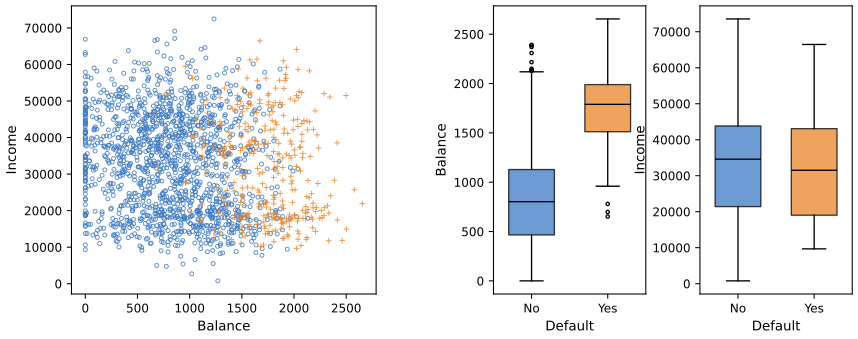
fig_4_1. Download: PDF · SVG4.2 Why Not Linear Regression?
pp. 131–132 Coding three diagnoses as \(Y=1,2,3\) (stroke, drug overdose, epileptic seizure) and fitting least squares would impose an order and equal spacing that the categories do not have; another, equally arbitrary, coding gives a different fit and different predictions. Only for an ordered response with roughly equal gaps (mild, moderate, severe) would such a coding be defensible.
With two classes the situation is better. Code \(Y\in\{0,1\}\), regress by least squares and predict class 1 when \(\hat Y>0.5\). Swapping the coding gives the same predictions, and \(X\hat\beta\) is an estimate of \(\Pr(Y=1\given X)\). But it is a poor one: a straight line leaves \([0,1]\) (Figure 4.2, left). So there are two reasons to prefer genuine classification methods: least squares cannot handle more than two unordered classes, and even for two classes it does not give sensible probabilities.
Filling the gap 4.1: what least squares on a 0/1 response estimates p. 132
(a) For a 0/1 response \[ \E(Y\given X=x)=0\cdot\Pr(Y=0\given x)+1\cdot\Pr(Y=1\given x)=\Pr(Y=1\given x) \], so regressing \(Y\) on \(X\) is estimating the class probability; least squares estimates its best linear approximation. (b) Swapping the coding replaces \(y_i\) by \(1-y_i\), whose least squares fit is \(1-\hat y_i\); so \(\hat y>0.5\) becomes \(1-\hat y\lt 0.5\) and the predicted class is the same. (c) The fitted values average to the proportion of ones, \(\bar y\) (0.0333 on the Default data), but are not confined to \([0,1]\): with balance alone, 31.2% of the fitted “probabilities” are negative.
Derivation
(a) is the definition of an expectation for a variable with values 0 and 1. (b) If \(\hat\beta\) minimises \(\sum_i(y_i-x_i^\T\beta)^2\) (with \(x_i\) including a leading 1), then \[ \sum_i\big((1-y_i)-x_i^\T\gamma\big)^2=\sum_i\big(y_i-x_i^\T(e_1-\gamma)\big)^2 \] with \(e_1=(1,0,\dots,0)^\T\), which is minimised by \(e_1-\gamma=\hat\beta\); so the new fitted values are \(1-x^\T\hat\beta\). (c) The normal equations \(\bX^\T(\by-\bX\hat\beta)=0\) include, for the intercept column, \(\sum_i(y_i-\hat y_i)=0\), so \(\frac1n\sum_i\hat y_i=\bar y\). The same identity holds for logistic regression (Result 4.1(c)), which is why the book finds the average fitted probability 0.0333 in both panels of Figure 4.2.
A caution about the book's next sentence. The book says that the classifications from linear regression on a binary response "will be the same" as those of LDA (Section 4.4). What is true is that the two methods produce the same direction \(\hat\beta\propto\hat\Sigma^{-1}(\hat\mu_1-\hat\mu_0)\) (Exercise 4.2 of the graduate book, Result 4.3 there); the cut-points differ unless the two classes have equal size. On the Default data with balance and student, the least squares fit and LDA have exactly proportional slopes, yet least squares with the cut 0.5 predicts no defaulter at all while LDA predicts 104 (Table 4.4). On the nearly balanced Smarket data the two rules agree on every day of 2005.
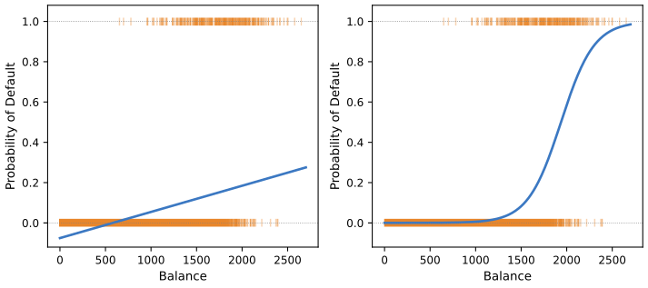
fig_4_2. Download: PDF · SVGDeeper: Statistical Learning: Theory and Methods, Section 4.2 (least squares on an indicator matrix for \(K\) classes, and how a class can be masked).
4.3 Logistic Regression
p. 133 Instead of modelling \(Y\) itself, logistic regression models the probability \(p(X)=\Pr(Y=1\given X)\), for the Default data \(\Pr(\text{default}=\text{Yes}\given\text{balance})\). A classification follows from a threshold: predict default when \(p(x)>0.5\), or, for a cautious lender, when \(p(x)>0.1\).
4.3.1 The Logistic Model
pp. 133–135 The linear model \(p(X)=\beta_0+\beta_1X\) (4.1) gives probabilities outside \([0,1]\). Logistic regression uses the logistic function, which maps the whole real line into \((0,1)\):
\[ p(X)=\frac{e^{\beta_0+\beta_1X}}{1+e^{\beta_0+\beta_1X}}. \tag{4.2} \]A little algebra turns (4.2) into statements about the odds and the log-odds:
\[ \frac{p(X)}{1-p(X)}=e^{\beta_0+\beta_1X}, \tag{4.3} \] \[ \log\Big(\frac{p(X)}{1-p(X)}\Big)=\beta_0+\beta_1X. \tag{4.4} \]Definition 4.1 (odds, log-odds, logit) pp. 134–135
For a probability \(p\in(0,1)\) the odds are \(p/(1-p)\in(0,\infty)\) and the log-odds or logit is \(\operatorname{logit}(p)=\log\{p/(1-p)\}\in\R\). The logistic function \(\sigma(\eta)=e^\eta/(1+e^\eta)=1/(1+e^{-\eta})\) is the inverse of the logit. Logistic regression is the model \(\operatorname{logit}p(x)=\beta_0+\beta_1x\): the log-odds are linear in \(x\).
Filling the gap 4.2: from (4.2) to (4.3) and (4.4), and what \(\beta_1\) means pp. 134–135
(a) (4.2), (4.3) and (4.4) are equivalent (Exercise 1). (b) Increasing \(X\) by one unit adds \(\beta_1\) to the log-odds and multiplies the odds by \(e^{\beta_1}\), whatever the starting value of \(X\). (c) The change in the probability itself is not constant: the slope of the curve is \(\mathrm{d}p/\mathrm{d}X=\beta_1\,p(X)\{1-p(X)\}\), largest (equal to \(\beta_1/4\)) where \(p=1/2\). Its sign is always the sign of \(\beta_1\).
Derivation
(a) Write \(\eta=\beta_0+\beta_1X\). From (4.2), \(1-p=1-\frac{e^\eta}{1+e^\eta}=\frac{1}{1+e^\eta}\), so \(p/(1-p)=e^\eta\), which is (4.3); taking logarithms gives (4.4). Conversely, if \(p/(1-p)=e^\eta\) then \(p=e^\eta(1-p)\), so \(p(1+e^\eta)=e^\eta\), which is (4.2).
(b) Odds at \(X+1\) divided by odds at \(X\): \(e^{\beta_0+\beta_1(X+1)}/e^{\beta_0+\beta_1X}=e^{\beta_1}\).
(c) \[ \sigma'(\eta)=\frac{e^\eta(1+e^\eta)-e^\eta e^\eta}{(1+e^\eta)^2}=\frac{e^\eta}{(1+e^\eta)^2}=\sigma(\eta)\{1-\sigma(\eta)\} \], and by the chain rule \(\mathrm{d}p/\mathrm{d}X=\beta_1\sigma'(\eta)\). The product \(p(1-p)\) is at most \(1/4\), at \(p=1/2\). For the Default fit of Table 4.1, \(\hat\beta_1=0.0055\), so near a balance of 1,937 (where \(\hat p=0.5\)) another \$100 of balance raises the probability of default by about \(100\times0.0055/4\approx0.14\); at a balance of 1,000 it raises it by only about 0.003. This is the "divide by 4" rule for reading logistic coefficients.
The book's examples: odds of 1/4 mean that on average one person in five defaults (\(p=0.2\)); odds of 9 mean nine in ten.
4.3.2 Estimating the Regression Coefficients
pp. 135–136 The coefficients are chosen by maximum likelihood: make the observed defaults as probable as possible under the model. With independent observations the likelihood is
\[ \ell(\beta_0,\beta_1)=\prod_{i:y_i=1}p(x_i)\prod_{i':y_{i'}=0}\big(1-p(x_{i'})\big). \tag{4.5} \]The book stops here ("the mathematical details of maximum likelihood are beyond the scope of this book"). The details are short, and they explain where the standard errors and \(z\) statistics of Table 4.1 come from.
Result 4.1 (the logistic likelihood: score, information, concavity) pp. 135–137
Let \(x_i=(1,x_{i1},\dots,x_{ip})^\T\), \(\beta=(\beta_0,\dots,\beta_p)^\T\), \(p_i=\sigma(x_i^\T\beta)\), \(\bX\) the \(n\times(p+1)\) matrix with rows \(x_i^\T\) and \(\bW=\diag\{p_i(1-p_i)\}\). Then
(a) the log-likelihood is \[ L(\beta)=\log\ell(\beta)=\sum_{i=1}^n\big\{y_i\,x_i^\T\beta-\log(1+e^{x_i^\T\beta})\big\} \];
(b) its gradient (the score) is \(\nabla L=\bX^\T(\by-\mathbf{p})\) and its Hessian is \(-\bX^\T\bW\bX\), which is negative definite when \(\bX\) has full column rank; so \(L\) is strictly concave and has at most one maximiser \(\hat\beta\), characterised by the score equations \(\bX^\T(\by-\hat{\mathbf{p}})=0\);
(c) because the first column of \(\bX\) is all ones, \(\sum_i\hat p_i=\sum_iy_i\): the fitted probabilities average to the observed proportion of ones;
(d) for large \(n\), \(\hat\beta\) is approximately normal with mean \(\beta\) and covariance \((\bX^\T\hat\bW\bX)^{-1}\) (the inverse Fisher information). The standard errors of Table 4.1 are the square roots of its diagonal, and \(z=\hat\beta_j/\mathrm{SE}(\hat\beta_j)\) is compared with \(\N(0,1)\).
Proof
(a) Each factor of (4.5) is \(p_i^{y_i}(1-p_i)^{1-y_i}\), so \[ L=\sum_i\{y_i\log p_i+(1-y_i)\log(1-p_i)\}=\sum_i\{y_i\log\frac{p_i}{1-p_i}+\log(1-p_i)\} \]. With \(\eta_i=x_i^\T\beta\), \(\log\frac{p_i}{1-p_i}=\eta_i\) by (4.4) and \(\log(1-p_i)=-\log(1+e^{\eta_i})\).
(b) \(\partial\log(1+e^{\eta})/\partial\eta=\sigma(\eta)\), so \[ \partial L/\partial\beta=\sum_i(y_i-p_i)x_i=\bX^\T(\by-\mathbf p) \]. Differentiating again, \(\partial p_i/\partial\beta=p_i(1-p_i)x_i\) (Filling the gap 4.2(c)), so the Hessian is \(-\sum_ip_i(1-p_i)x_ix_i^\T=-\bX^\T\bW\bX\). For any \(v\ne0\), \(v^\T\bX^\T\bW\bX v=\sum_ip_i(1-p_i)(x_i^\T v)^2>0\), because the weights are positive and \(\bX v\ne0\) when \(\bX\) has full column rank. A strictly concave function has at most one maximiser, at the zero of its gradient.
(c) The first score equation (the derivative in \(\beta_0\)) reads \(\sum_i(y_i-\hat p_i)=0\).
(d) This is the general large-sample theory of maximum likelihood: \(\hat\beta\approx\N(\beta,\mathcal I(\beta)^{-1})\) with the information \(\mathcal I(\beta)=-\E\,\nabla^2L=\bX^\T\bW\bX\) (here the Hessian does not involve \(\by\), so the observed and expected information coincide). A sketch: expand the score around the true \(\beta\), \[ 0=\nabla L(\hat\beta)\approx\nabla L(\beta)-\mathcal I(\beta)(\hat\beta-\beta) \], so \(\hat\beta-\beta\approx\mathcal I^{-1}\nabla L(\beta)\); the score is a sum of independent terms with mean 0 and covariance \(\mathcal I\), hence approximately normal by the central limit theorem, and \(\mathcal I^{-1}\nabla L\) has covariance \(\mathcal I^{-1}\mathcal I\mathcal I^{-1}=\mathcal I^{-1}\). ∎
When the maximum does not exist. If some hyperplane separates the 0s from the 1s perfectly, the likelihood increases towards 1 as \(\|\beta\|\to\infty\) along the separating direction, and there is no finite maximiser; software then reports huge coefficients and the warning "fitted probabilities numerically 0 or 1" (it appears in the Caravan lab, Section 4.7.6). This is the instability the book mentions at the start of Section 4.4. ∎
Algorithm 4.1 (Newton-Raphson for logistic regression, also called iteratively reweighted least squares)
- Start from \(\beta=0\) (all probabilities 1/2).
- Compute \(\eta_i=x_i^\T\beta\), \(p_i=\sigma(\eta_i)\) and weights \(w_i=p_i(1-p_i)\).
- Update \(\beta\leftarrow\beta+(\bX^\T\bW\bX)^{-1}\bX^\T(\by-\mathbf p)\). Equivalently, \(\beta\) is the weighted least squares fit of the working response \(z_i=\eta_i+(y_i-p_i)/w_i\) on \(x_i\) with weights \(w_i\).
- Repeat steps 2–3 until \(\beta\) stops changing; report \(\mathrm{SE}(\hat\beta_j)=\{(\bX^\T\bW\bX)^{-1}\}_{jj}^{1/2}\).
This is what R's glm(..., family = binomial) and Python's statsmodels GLM do (R calls it "Fisher scoring"; for the logistic model Fisher scoring and Newton's method coincide). On the Default data it converges in 10 steps from \(\beta=0\); logistic_fit in ch04_classification.py is a direct transcription, and its coefficients and standard errors equal those of statsmodels to 13 digits.
Deeper: Statistical Learning: Theory and Methods, Section 4.4.1 (Result 4.8: score, Hessian, Newton–Raphson as IRLS, and step halving) and Section 4.4.3 (Wald, score and likelihood ratio tests, the deviance). See also: Foundations of Deep Learning, Result 5.16 (the same gradient and Hessian as a cross-entropy loss) and Result 5.17 (separable data).
pp. 136–137 Table 4.1 is the fit of default on balance. The \(z\) statistic plays the role of the \(t\) statistic of Chapter 3: a large \(|z|\) is evidence against \(H_0:\beta_1=0\), under which \(p(X)=e^{\beta_0}/(1+e^{\beta_0})\) does not depend on balance. The intercept only adjusts the average fitted probability to the default rate (Result 4.1(c)).
| Table 4.1 (recomputed) | Coefficient | Std. error | z-statistic | p-value |
|---|---|---|---|---|
| Intercept | −10.6513 | 0.3612 | −29.5 | <0.0001 |
| balance | 0.0055 | 0.0002 | 24.9 | <0.0001 |
Every entry agrees with the book. The full-precision slope is 0.0054989, so the "divide by 4" rule of Filling the gap 4.2 gives a maximal slope of 0.00137 per dollar.
4.3.3 Making Predictions
pp. 136–137 Plugging the estimates into (4.2): a balance of \$1,000 gives \[ \hat p=e^{-10.6513+0.0055\times1000}/(1+e^{-10.6513+0.0055\times1000})=0.00576 \], below 1%, and a balance of \$2,000 gives 0.586. Recomputed with the unrounded coefficients these are 0.00575 and 0.586.
A qualitative predictor enters through a dummy variable. Regressing default on student status alone (Table 4.2) gives a positive coefficient: students default more often.
| Table 4.2 (recomputed) | Coefficient | Std. error | z-statistic | p-value |
|---|---|---|---|---|
| Intercept | −3.5041 | 0.0707 | −49.55 | <0.0001 |
| student[Yes] | 0.4049 | 0.1150 | 3.52 | 0.0004 |
The fitted probabilities are \(\sigma(-3.5041+0.4049)=0.0431\) for students and \(\sigma(-3.5041)=0.0292\) for non-students. With a single dummy predictor these are exactly the observed default rates in the two groups (127 of 2,944 students and 206 of 7,056 non-students), because the score equations of Result 4.1 force the fitted and observed counts to agree within each group.
4.3.4 Multiple Logistic Regression
pp. 137–139 With \(p\) predictors,
\[ \log\Big(\frac{p(X)}{1-p(X)}\Big)=\beta_0+\beta_1X_1+\dots+\beta_pX_p, \tag{4.6} \] \[ p(X)=\frac{e^{\beta_0+\beta_1X_1+\dots+\beta_pX_p}}{1+e^{\beta_0+\beta_1X_1+\dots+\beta_pX_p}}, \tag{4.7} \]fitted by maximum likelihood exactly as before (Algorithm 4.1 works for any \(p\)). Table 4.3 uses balance, income (in thousands of dollars) and student status.
| Table 4.3 (recomputed) | Coefficient | Std. error | z-statistic | p-value |
|---|---|---|---|---|
| Intercept | −10.8690 | 0.4923 | −22.08 | <0.0001 |
| balance | 0.0057 | 0.0002 | 24.74 | <0.0001 |
| income | 0.0030 | 0.0082 | 0.37 | 0.7115 |
| student[Yes] | −0.6468 | 0.2363 | −2.74 | 0.0062 |
All entries agree with the book except the standard error of the student coefficient, which is 0.236253 in both R and Python (so 0.2363, where the book prints 0.2362). The surprise is the sign: student status raises the risk on its own (Table 4.2) but lowers it once balance is in the model. Figure 4.3 explains why.
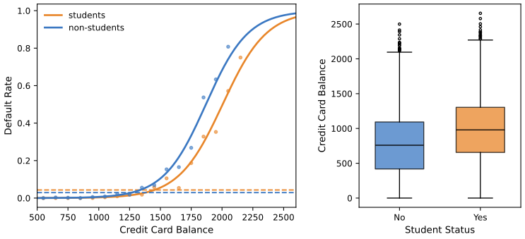
fig_4_3. Download: PDF · SVGFilling the gap 4.3: how a coefficient can change sign (confounding) pp. 138–139
The marginal default rate of a group is the average of its balance-specific rates, weighted by how that group's balances are distributed:
\[ \Pr(D\given S)=\int\Pr(D\given S,b)\,f(b\given S)\,\mathrm{d}b. \]If students have a lower rate at every balance, \(\Pr(D\given S{=}1,b)\lt \Pr(D\given S{=}0,b)\), but their balances are shifted towards the region where \(\Pr(D\given\cdot,b)\) is large, the student average can still be larger. That is exactly Figure 4.3: the conditional comparison (Table 4.3, negative coefficient) and the marginal comparison (Table 4.2, positive coefficient) answer different questions, and both are correct.
A two-group calculation
Suppose balances are either "low" (default rate 1% for non-students, 0.5% for students) or "high" (20% and 15%). If 10% of non-students and 30% of students have high balances, the marginal rates are \(0.9\times0.01+0.1\times0.20=0.029\) for non-students and \(0.7\times0.005+0.3\times0.15=0.0485\) for students. Students are safer within each balance group and riskier overall. The phenomenon is known as Simpson's paradox; the book calls the underlying situation confounding: student status is associated with balance, and balance drives default. A lender who knows the balance should use the conditional comparison; a lender who does not should use the marginal one.
Predictions from Table 4.3: a student with balance \$1,500 and income \$40,000 has \(\hat p=0.058\) (4.8), a non-student with the same balance and income 0.105 (4.9); income enters as 40 because the model was fitted in thousands of dollars. Recomputed: 0.0579 and 0.1050.
4.3.5 Multinomial Logistic Regression
pp. 140–141 For \(K>2\) classes choose a baseline, say class \(K\), and set, for \(k=1,\dots,K-1\),
\[ \Pr(Y=k\given X=x)=\frac{e^{\beta_{k0}+\beta_{k1}x_1+\dots+\beta_{kp}x_p}}{1+\sum_{l=1}^{K-1}e^{\beta_{l0}+\beta_{l1}x_1+\dots+\beta_{lp}x_p}}, \tag{4.10} \] \[ \Pr(Y=K\given X=x)=\frac{1}{1+\sum_{l=1}^{K-1}e^{\beta_{l0}+\beta_{l1}x_1+\dots+\beta_{lp}x_p}}, \tag{4.11} \]so that
\[ \log\Big(\frac{\Pr(Y=k\given X=x)}{\Pr(Y=K\given X=x)}\Big)=\beta_{k0}+\beta_{k1}x_1+\dots+\beta_{kp}x_p. \tag{4.12} \]In the softmax coding all classes are treated alike,
\[ \Pr(Y=k\given X=x)=\frac{e^{\beta_{k0}+\beta_{k1}x_1+\dots+\beta_{kp}x_p}}{\sum_{l=1}^Ke^{\beta_{l0}+\beta_{l1}x_1+\dots+\beta_{lp}x_p}}, \tag{4.13} \] \[ \log\Big(\frac{\Pr(Y=k\given X=x)}{\Pr(Y=k'\given X=x)}\Big)=(\beta_{k0}-\beta_{k'0})+(\beta_{k1}-\beta_{k'1})x_1+\dots+(\beta_{kp}-\beta_{k'p})x_p. \tag{4.14} \]Result 4.2 (the baseline and softmax codings are one model) pp. 140–141
(a) (4.10)–(4.11) imply (4.12), and the probabilities sum to one. (b) The softmax model (4.13) is unchanged if the same vector \(c\) is added to every \(\beta_k\); so only the differences \(\beta_k-\beta_{k'}\) are determined by the data, which is (4.14). Setting \(\beta_K=0\) turns (4.13) into (4.10)–(4.11). (c) Hence the choice of baseline, or of coding, changes the coefficients but not the fitted probabilities, the log-odds between any two classes, the likelihood or the predictions. A coefficient \(\beta_{kj}\) in the baseline coding is the change in the log-odds of class \(k\) against the baseline per unit of \(x_j\).
Proof
(a) Divide (4.10) by (4.11): the denominators cancel and the ratio is \(e^{\beta_{k0}+\dots+\beta_{kp}x_p}\). Adding (4.10) over \(k\lt K\) and (4.11) gives \[ \big(\sum_{l\lt K}e^{\eta_l}+1\big)/\big(1+\sum_{l\lt K}e^{\eta_l}\big)=1 \].
(b) Write \(\eta_k=\beta_{k0}+\beta_k^\T x\) and replace \((\beta_{k0},\beta_k)\) by \((\beta_{k0}+c_0,\beta_k+c)\) for every \(k\). Each \(\eta_k\) gains \(c_0+c^\T x\), so numerator and denominator of (4.13) are both multiplied by \(e^{c_0+c^\T x}\). Choosing \(c=-\beta_K\) makes the \(K\)th exponent 0, i.e. \(e^0=1\) in the denominator: that is (4.10)–(4.11) with coefficients \(\beta_k-\beta_K\).
(c) Changing the baseline from \(K\) to \(m\) is the same reparametrisation with \(c=-\beta_m\); the probabilities are a function of the differences only. Numerically: fitting a three-class model with each class in turn as the baseline gives fitted probabilities equal to \(10^{-15}\). ∎
Deeper: Statistical Learning: Theory and Methods, Section 4.4 (the \(K\)-class model fitted by Newton's method). See also: Foundations of Deep Learning, Section 5.4.4 and Result 5.18 (the softmax as the output layer of a network, which is why Chapter 10 uses this coding).
4.4 Generative Models for Classification
pp. 141–142 Logistic regression models \(\Pr(Y\given X)\) directly. The alternative is to model how \(X\) is distributed within each class and turn this around with Bayes' theorem. Let \(\pi_k\) be the prior probability of class \(k\) and \(f_k(x)\) the density of \(X\) in class \(k\). Then
\[ \Pr(Y=k\given X=x)=\frac{\pi_kf_k(x)}{\sum_{l=1}^K\pi_lf_l(x)}, \tag{4.15} \]abbreviated \(p_k(x)\), the posterior probability of class \(k\). The priors are easy to estimate (class proportions, \(\hat\pi_k=n_k/n\), if the sample is random); the densities are not, and the three methods of this section differ only in what they assume about them. Why bother, when logistic regression exists? The book gives three reasons: logistic estimates are unstable when the classes are well separated (no finite maximum, Result 4.1); with roughly normal classes and few data the generative methods can be more accurate; and they extend naturally to \(K>2\).
See also (companion course): Foundations of Deep Learning, Section 5.3 (generative classifiers, and why their posterior is a sigmoid or softmax of a linear function).
4.4.1 Linear Discriminant Analysis for p = 1
pp. 142–145 Assume one predictor, normal within each class,
\[ f_k(x)=\frac{1}{\sqrt{2\pi}\sigma_k}\exp\Big(-\frac{1}{2\sigma_k^2}(x-\mu_k)^2\Big), \tag{4.16} \]with a common variance \(\sigma_1^2=\dots=\sigma_K^2=\sigma^2\). Then (4.15) becomes
\[ p_k(x)=\frac{\pi_k\frac{1}{\sqrt{2\pi}\sigma}\exp\big(-\frac{1}{2\sigma^2}(x-\mu_k)^2\big)}{\sum_{l=1}^K\pi_l\frac{1}{\sqrt{2\pi}\sigma}\exp\big(-\frac{1}{2\sigma^2}(x-\mu_l)^2\big)}, \tag{4.17} \]and the Bayes classifier assigns \(x\) to the class with the largest
\[ \delta_k(x)=x\cdot\frac{\mu_k}{\sigma^2}-\frac{\mu_k^2}{2\sigma^2}+\log(\pi_k). \tag{4.18} \]Result 4.3 (the linear discriminant from Bayes' theorem; Exercise 2) pp. 142–143
(a) Maximising (4.17) over \(k\) is the same as maximising (4.18). (b) For \(K=2\) the Bayes decision boundary is the point
\[ x^*=\frac{\mu_1+\mu_2}{2}+\frac{\sigma^2\log(\pi_2/\pi_1)}{\mu_1-\mu_2}, \]which reduces to \[ x^*=\frac{\mu_1^2-\mu_2^2}{2(\mu_1-\mu_2)}=\frac{\mu_1+\mu_2}{2} \] (4.19) when \(\pi_1=\pi_2\). (c) With equal priors the Bayes error rate is \(\Phi(-\Delta/2)\), where \(\Delta=|\mu_1-\mu_2|/\sigma\) and \(\Phi\) is the standard normal distribution function.
Proof
(a) The denominator of (4.17) is the same for every \(k\), and so is the factor \(1/(\sqrt{2\pi}\sigma)\); since the logarithm is increasing, maximising \(p_k(x)\) is maximising \[ \log\pi_k-\frac{(x-\mu_k)^2}{2\sigma^2}=\log\pi_k-\frac{x^2}{2\sigma^2}+\frac{x\mu_k}{\sigma^2}-\frac{\mu_k^2}{2\sigma^2} \]. The term \(-x^2/(2\sigma^2)\) does not depend on \(k\) and can be dropped, which leaves (4.18). The cancellation of \(x^2\) is what makes the rule linear; it relies on the common variance (Exercise 3 shows what happens without it).
(b) \(\delta_1(x)=\delta_2(x)\) reads \[ x(\mu_1-\mu_2)/\sigma^2=(\mu_1^2-\mu_2^2)/(2\sigma^2)+\log(\pi_2/\pi_1) \]; divide by \((\mu_1-\mu_2)/\sigma^2\) and use \(\mu_1^2-\mu_2^2=(\mu_1-\mu_2)(\mu_1+\mu_2)\). A larger prior for class 2 moves the boundary towards \(\mu_1\), enlarging the region of class 2.
(c) Take \(\mu_1\lt \mu_2\). An observation from class 1 is misclassified when \(X>x^*=(\mu_1+\mu_2)/2\), with probability \(\Pr(Z>(\mu_2-\mu_1)/(2\sigma))=\Phi(-\Delta/2)\); by symmetry the same holds for class 2, and the average over the two equally likely classes is \(\Phi(-\Delta/2)\). In the example of Figure 4.4, \(\mu_{1,2}=\mp1.25\), \(\sigma=1\), \(\Delta=2.5\), and the Bayes error is \(\Phi(-1.25)=0.1056\), the book's 10.6%. ∎
In practice the parameters are unknown, and linear discriminant analysis (LDA) plugs in
\[ \hat\mu_k=\frac{1}{n_k}\sum_{i:y_i=k}x_i,\qquad\hat\sigma^2=\frac{1}{n-K}\sum_{k=1}^K\sum_{i:y_i=k}(x_i-\hat\mu_k)^2, \tag{4.20} \] \[ \hat\pi_k=n_k/n, \tag{4.21} \]and classifies to the largest
\[ \hat\delta_k(x)=x\cdot\frac{\hat\mu_k}{\hat\sigma^2}-\frac{\hat\mu_k^2}{2\hat\sigma^2}+\log(\hat\pi_k). \tag{4.22} \]Filling the gap 4.4: where the estimates (4.20)–(4.21) come from p. 144
They are the maximum likelihood estimates of the generative model, except that the variance is divided by \(n-K\) instead of \(n\), which makes it unbiased. The pooled variance is a weighted average of the class variances: \(\hat\sigma^2=\sum_k\frac{n_k-1}{n-K}s_k^2\), where \(s_k^2\) is the sample variance of class \(k\).
Derivation
The joint log-likelihood of the pairs \((x_i,y_i)\) is \(\sum_i\log\pi_{y_i}+\sum_i\log f_{y_i}(x_i)\). The first sum involves only the \(\pi_k\): maximising \(\sum_kn_k\log\pi_k\) subject to \(\sum_k\pi_k=1\) (a Lagrange multiplier, or Gibbs' inequality) gives \(\hat\pi_k=n_k/n\). The second sum is \[ -\frac{n}{2}\log(2\pi\sigma^2)-\frac{1}{2\sigma^2}\sum_k\sum_{i:y_i=k}(x_i-\mu_k)^2 \]. For fixed \(\sigma\) each \(\mu_k\) minimises a sum of squares, so \(\hat\mu_k\) is the class mean; then setting the derivative in \(\sigma^2\) to zero gives \[ \hat\sigma^2_{\rm ML}=\frac1n\sum_k\sum_{i:y_i=k}(x_i-\hat\mu_k)^2 \]. Each class sum of squares has expectation \((n_k-1)\sigma^2\), so the total has expectation \((n-K)\sigma^2\), and dividing by \(n-K\) removes the bias. With \(n=10{,}000\) the difference is negligible; with 20 points per class (Figure 4.4) it is 2.5%.
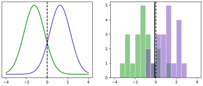
fig_4_4. Download: PDF · SVG4.4.2 Linear Discriminant Analysis for p > 1
pp. 145–152 With \(p\) predictors, assume \(X\) is multivariate normal in each class, \(X\sim\N(\mu_k,\Sigma)\), with class-specific mean vectors and one covariance matrix \(\Sigma\) shared by all classes:
\[ f(x)=\frac{1}{(2\pi)^{p/2}|\Sigma|^{1/2}}\exp\Big(-\frac12(x-\mu)^\T\Sigma^{-1}(x-\mu)\Big). \tag{4.23} \]Each margin is normal; correlation and unequal variances turn the circular contours into ellipses (Figure 4.5). The Bayes classifier now assigns \(x\) to the class with the largest
\[ \delta_k(x)=x^\T\Sigma^{-1}\mu_k-\frac12\mu_k^\T\Sigma^{-1}\mu_k+\log\pi_k, \tag{4.24} \]and the boundary between classes \(k\) and \(l\) is the set where \(\delta_k=\delta_l\); with equal priors,
\[ x^\T\Sigma^{-1}\mu_k-\frac12\mu_k^\T\Sigma^{-1}\mu_k=x^\T\Sigma^{-1}\mu_l-\frac12\mu_l^\T\Sigma^{-1}\mu_l. \tag{4.25} \]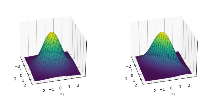
fig_4_5. Download: PDF · SVGFilling the gap 4.5: from (4.23) to (4.24), the "little bit of algebra" p. 147
The quadratic term in \(x\) cancels because \(\Sigma\) is shared, so the discriminant is linear. The 95% ellipses of Figure 4.6 are the sets \((x-\mu_k)^\T\Sigma^{-1}(x-\mu_k)=\chi^2_{2,0.95}=5.99\), i.e. Mahalanobis radius 2.448.
Derivation
As in Result 4.3, drop the common denominator of (4.15) and the common constant \((2\pi)^{-p/2}|\Sigma|^{-1/2}\), and take logarithms: the class maximises \(\log\pi_k-\frac12(x-\mu_k)^\T\Sigma^{-1}(x-\mu_k)\). Expand the quadratic form, using the symmetry of \(\Sigma^{-1}\) (so \(x^\T\Sigma^{-1}\mu_k=\mu_k^\T\Sigma^{-1}x\)):
\[ (x-\mu_k)^\T\Sigma^{-1}(x-\mu_k)=x^\T\Sigma^{-1}x-2x^\T\Sigma^{-1}\mu_k+\mu_k^\T\Sigma^{-1}\mu_k. \]The first term is the same for every class and drops out; what is left, times \(-\frac12\), plus \(\log\pi_k\), is (4.24). For \(p=1\), \(\Sigma=\sigma^2\) and (4.24) is (4.18). For the ellipses: if \(X\sim\N(\mu,\Sigma)\) then \((X-\mu)^\T\Sigma^{-1}(X-\mu)\) is a sum of \(p\) squared independent standard normals (write \(X-\mu=\Sigma^{1/2}Z\)), so it has a \(\chi^2_p\) distribution, and the region inside the level \(\chi^2_{p,0.95}\) holds 95% of the probability.
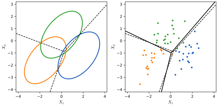
fig_4_6. Download: PDF · SVGpp. 147–149 LDA estimates \(\mu_k\) by the class means, \(\pi_k\) by \(n_k/n\) and \(\Sigma\) by the pooled within-class covariance \[ \hat\Sigma=\frac{1}{n-K}\sum_k\sum_{i:y_i=k}(x_i-\hat\mu_k)(x_i-\hat\mu_k)^\T \], and classifies to the largest \(\hat\delta_k(x)\). On the Default data with balance and student status (a 0/1 variable, so certainly not normal; LDA is often robust to this), LDA makes 275 errors among 10,000 people, a training error rate of 2.75%. Two caveats: training error flatters a method (here only mildly, with \(p=2\) and \(n=10{,}000\)), and the trivial rule "nobody defaults" already has an error rate of 3.33%. The confusion matrix (Table 4.4) shows where the errors are.
| Table 4.4 (recomputed) | True No | True Yes | Total |
|---|---|---|---|
| Predicted No | 9,644 | 252 | 9,896 |
| Predicted Yes | 23 | 81 | 104 |
| Total | 9,667 | 333 | 10,000 |
Only 23 of 9,667 non-defaulters are flagged, but 252 of the 333 defaulters (75.7%) are missed: the sensitivity (share of defaulters caught) is 81/333 = 24.3% and the specificity (share of non-defaulters cleared) is 1 − 23/9,667 = 99.8%.
Definition 4.2 (the confusion matrix and its rates; Tables 4.6 and 4.7) pp. 151–152
Call the class of interest (default, disease) "positive". Among the \(P\) true positives and \(N\) true negatives, a classifier produces true positives TP, false negatives FN, false positives FP and true negatives TN, with \(P^*=\mathrm{TP}+\mathrm{FP}\) predicted positives and \(N^*=\mathrm{TN}+\mathrm{FN}\) predicted negatives. Then:
| Name | Definition | Also called |
|---|---|---|
| false positive rate | FP/N | type I error, 1 − specificity |
| true positive rate | TP/P | 1 − type II error, power, sensitivity, recall |
| positive predictive value | TP/P* | precision, 1 − false discovery proportion |
| negative predictive value | TN/N* |
The first two divide by the true class sizes, the last two by the predicted class sizes. For Table 4.4: false positive rate 0.24%, sensitivity 24.3%, positive predictive value 81/104 = 77.9%, negative predictive value 9,644/9,896 = 97.5%.
pp. 148–150 Why is the sensitivity so low? LDA approximates the Bayes classifier, which minimises the total number of errors whatever their kind; it predicts default only when \(\Pr(\text{default}\given x)>0.5\) (4.26). A lender may care far more about missed defaulters, and can lower the threshold, say to \(\Pr(\text{default}\given x)>0.2\) (4.27). Table 4.5 is the result.
| Table 4.5 (recomputed) | True No | True Yes | Total |
|---|---|---|---|
| Predicted No | 9,432 | 138 | 9,570 |
| Predicted Yes | 235 | 195 | 430 |
| Total | 9,667 | 333 | 10,000 |
Now only 138 defaulters (41.4%) are missed, at the cost of 235 false alarms; the overall error rises slightly to 3.73%. Figure 4.7 shows the whole trade-off and Figure 4.8 summarises it over all thresholds.
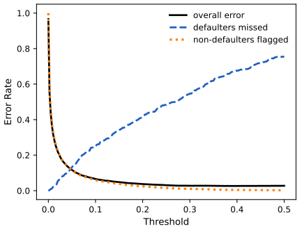
fig_4_7. Download: PDF · SVGFilling the gap 4.6: why 0.5, and which threshold for unequal costs pp. 149–150
(a) If the posterior \(p(x)=\Pr(Y=1\given x)\) were known, the rule "predict 1 when \(p(x)>1/2\)" would minimise the error rate. (b) If a missed positive costs \(c_{\rm FN}\) and a false alarm costs \(c_{\rm FP}\), the expected cost is minimised by predicting 1 when \(p(x)>c_{\rm FP}/(c_{\rm FP}+c_{\rm FN})\). A missed defaulter that costs ten false alarms gives the threshold \(1/11=0.091\). (c) With an estimated posterior the optimality is only approximate: on the Default training data LDA's overall error is 2.75% at 0.5 but 2.63% near 0.37–0.40.
Derivation
(a, b) At a given \(x\), predicting 1 costs \(c_{\rm FP}\) with probability \(1-p(x)\) (if \(Y=0\)), and predicting 0 costs \(c_{\rm FN}\) with probability \(p(x)\). Predict 1 exactly when \(c_{\rm FP}\{1-p(x)\}\lt c_{\rm FN}\,p(x)\), i.e. \(p(x)>c_{\rm FP}/(c_{\rm FP}+c_{\rm FN})\). Doing the best thing at every \(x\) minimises the average cost over \(x\). Equal costs give 1/2, which is the Bayes classifier of Chapter 2.
(c) The argument assumes the true posterior. LDA's posterior is estimated, from a model that is wrong for the binary student variable, so the error-minimising cut on the training data need not be 0.5; the difference here is 12 people in 10,000. The book's sentence that the threshold 0.5 "minimizes the overall error rate" in Figure 4.7 is true of the Bayes classifier, and only approximately of the LDA fit. With the 1/11 threshold of (b), LDA flags 894 people, catches 253 of the 333 defaulters (sensitivity 76.0%) and has an overall error of 7.21%.
pp. 150–151 The ROC curve (receiver operating characteristic) plots the true positive rate against the false positive rate as the threshold runs from 1 down to 0 (Figure 4.8). A perfect classifier hugs the top left corner; a classifier that ignores \(x\) follows the diagonal. The area under the curve (AUC) summarises it: 0.95 for LDA on the Default data, against 0.5 for chance. The ROC curve of logistic regression on the same inputs is virtually the same (AUC 0.9495 against 0.9496).
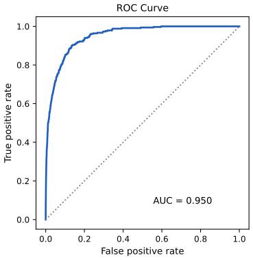
fig_4_8. Download: PDF · SVGResult 4.4 (what the AUC measures) p. 151
Let a classifier give each observation a score \(s\) (for instance \(\hat p(x)\)), and draw one positive and one negative observation at random. Then
\[ \mathrm{AUC}=\Pr(s_{+}>s_{-})+\tfrac12\Pr(s_{+}=s_{-}). \]Consequently the AUC is unchanged by any increasing transformation of the score (the posterior, the log-odds and the LDA discriminant all give the same ROC curve), a score unrelated to the class has AUC 1/2, and the AUC equals the Mann–Whitney statistic \(U/(n_+n_-)\).
Proof
Sort the distinct scores from high to low. Lowering the threshold past a score value \(t\) moves the ROC curve right by \(1/n_-\) times the number of negatives at \(t\) and up by \(1/n_+\) times the number of positives at \(t\) (a diagonal segment when both are present). The area under the curve is therefore a sum over the negatives: each negative with score \(t\) contributes \(\frac{1}{n_-}\) times the height of the curve at that step, which is the fraction of positives with a larger score, plus half the fraction with an equal score (the trapezoid under a diagonal piece). Averaging over the negatives gives \[ \frac{1}{n_+n_-}\sum_{\text{pairs}}\{\mathbf 1(s_+>s_-)+\frac12\mathbf 1(s_+=s_-)\} \], which is the stated probability for the empirical distribution. An increasing transformation preserves every comparison \(s_+>s_-\). If \(s\) is independent of the class, \(s_+\) and \(s_-\) are exchangeable and the probability is 1/2. Numerically, for the LDA scores the rank formula and the trapezoidal area of the ROC curve agree to \(10^{-12}\). ∎
The ROC curve and the AUC are computed here on the training data, as in the book. The book's remark that a classifier no better than chance has AUC 0.5 "when evaluated on an independent test set" matters: on the training data even a useless but flexible method can look better than chance.
Deeper: Statistical Learning: Theory and Methods, Section 4.3 (Result 4.2, the linear log-odds of Gaussian classes; regularised and reduced-rank LDA). See also: Foundations of Deep Learning, Section 5.2.6 and Result 5.9 (properties of ROC curves) and Result 5.6 (minimum expected loss, the cost-weighted threshold).
4.4.3 Quadratic Discriminant Analysis
pp. 152–153 Quadratic discriminant analysis (QDA) keeps the normal classes but lets each have its own covariance, \(X\sim\N(\mu_k,\Sigma_k)\). The Bayes classifier then maximises
\[ \begin{aligned}\delta_k(x)&=-\tfrac12(x-\mu_k)^\T\Sigma_k^{-1}(x-\mu_k)-\tfrac12\log|\Sigma_k|+\log\pi_k\\&=-\tfrac12x^\T\Sigma_k^{-1}x+x^\T\Sigma_k^{-1}\mu_k-\tfrac12\mu_k^\T\Sigma_k^{-1}\mu_k-\tfrac12\log|\Sigma_k|+\log\pi_k,\end{aligned} \tag{4.28} \]which is quadratic in \(x\); QDA plugs in the class means, the class covariance matrices (divisor \(n_k-1\)) and \(n_k/n\).
Result 4.5 (QDA, and the price of flexibility; Exercise 3) pp. 152–153
(a) (4.28) follows from (4.15) and (4.23) with \(\Sigma_k\) in place of \(\Sigma\); the term \(-\frac12x^\T\Sigma_k^{-1}x\) no longer cancels, so the boundaries are quadratic curves (conics when \(p=2\)) unless all \(\Sigma_k\) are equal. (b) QDA estimates \(Kp(p+1)/2\) covariance parameters, LDA only \(p(p+1)/2\); with \(p=50\) that is \(1{,}275\) per class. On the log-odds scale (Section 4.5.1) LDA has \((K-1)(p+1)\) free coefficients and QDA \((K-1)\{1+p+p(p+1)/2\}\).
Proof
(a) As in Filling the gap 4.5, but the normalising constant \(|\Sigma_k|^{-1/2}\) now depends on \(k\) and contributes \(-\frac12\log|\Sigma_k|\), and expanding the quadratic form leaves \(-\frac12x^\T\Sigma_k^{-1}x\), which differs between classes. For \(p=1\) (Exercise 3) \[ \delta_k(x)=-\frac{x^2}{2\sigma_k^2}+\frac{x\mu_k}{\sigma_k^2}-\frac{\mu_k^2}{2\sigma_k^2}-\log\sigma_k+\log\pi_k \], and \(\delta_k=\delta_l\) is a quadratic equation in \(x\) whose \(x^2\) coefficient \(\frac{1}{2\sigma_l^2}-\frac{1}{2\sigma_k^2}\) vanishes only if \(\sigma_k=\sigma_l\); a class with a small variance then owns an interval and the other class both tails.
(b) A symmetric \(p\times p\) matrix has \(p\) diagonal and \(p(p-1)/2\) off-diagonal entries, \(p(p+1)/2\) in all. The log-odds count is the number of coefficients in (4.32) and (4.33) below: a constant, \(p\) linear terms and, for QDA, \(p(p+1)/2\) distinct products \(x_jx_l\) with \(j\le l\), for each of the \(K-1\) non-baseline classes. ∎
This is the bias–variance trade-off of Chapter 2: LDA is less flexible and has lower variance, so it tends to win with few training points; QDA wins when \(n\) is large or the covariances clearly differ. Figure 4.9 shows both cases.
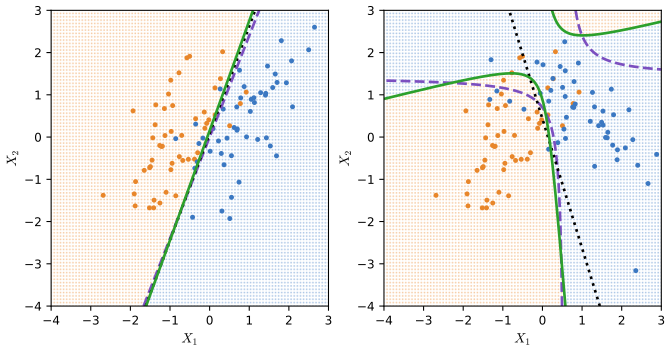
fig_4_9. Download: PDF · SVGDeeper: Statistical Learning: Theory and Methods, Section 4.3 (Filling the gap 4.4: QDA and counting parameters) and Section 4.3.1 (regularised discriminant analysis, a compromise between LDA and QDA). See also: Foundations of Deep Learning, Filling the gap 5.8 (different covariances give quadratic boundaries).
4.4.4 Naive Bayes
pp. 153–158 Estimating a \(p\)-dimensional density is hard because of the dependence between the predictors. Naive Bayes simply assumes it away: within each class the predictors are independent,
\[ f_k(x)=f_{k1}(x_1)\times f_{k2}(x_2)\times\dots\times f_{kp}(x_p), \tag{4.29} \]so that
\[ \Pr(Y=k\given X=x)=\frac{\pi_k\times f_{k1}(x_1)\times f_{k2}(x_2)\times\dots\times f_{kp}(x_p)}{\sum_{l=1}^K\pi_l\times f_{l1}(x_1)\times f_{l2}(x_2)\times\dots\times f_{lp}(x_p)}. \tag{4.30} \]Each one-dimensional \(f_{kj}\) can be estimated in the simplest way that suits the predictor: a normal density for a quantitative \(X_j\) (this is QDA with diagonal covariance matrices), a histogram or a kernel density estimate, or, for a qualitative \(X_j\), the proportions of its levels within class \(k\) (e.g. 0.32, 0.55, 0.13 for a three-level predictor seen 32, 55 and 13 times among 100 class-\(k\) observations). The independence assumption is rarely true, but it trades some bias for a large reduction in variance, which pays when \(n\) is not large relative to \(p\).
Filling the gap 4.7: the toy example, and the Default tables pp. 155–158
(a) With \(\hat\pi_1=\hat\pi_2=1/2\) and the book's density values at \(x^*=(0.4,1.5,1)\), \(\hat f_{11}=0.368\), \(\hat f_{12}=0.484\), \(\hat f_{13}=0.226\) and \(\hat f_{21}=0.030\), \(\hat f_{22}=0.130\), \(\hat f_{23}=0.616\), (4.30) gives
\[ \Pr(Y=1\given x^*)=\frac{0.368\times0.484\times0.226}{0.368\times0.484\times0.226+0.030\times0.130\times0.616}=\frac{0.04025}{0.04025+0.00240}=0.944. \](b) Tables 4.8 and 4.9 are reproduced exactly by naive Bayes on three predictors: balance and income with normal densities (standard deviations with divisor \(n_k-1\), as R's naiveBayes()) and student status with its class proportions.
Details
(a) The priors cancel. The prior-weighted numerators are \(0.5\times0.04025\) and \(0.5\times0.00240\); their ratio, about 17 to 1, is the posterior odds. In the simulated example of Figure 4.10 (my settings, stated in the code) the six kernel density values at \(x^*\) are 0.361, 0.365, 0.200 and 0.111, 0.008, 0.520, and the posterior is 0.983.
(b) With balance, income and student: Table 4.8 (threshold 0.5) has 9,615 / 241 / 52 / 92 and Table 4.9 (threshold 0.2) has 9,320 / 128 / 347 / 205, exactly as printed. With only balance and student (\(p=2\), as for LDA) the counts are different (9,621 / 244 / 46 / 89 at 0.5). Treating the 0/1 student variable as normal changes a few counts too (9,610 / 239 / 57 / 94). The text's "\(p=4\)" (R edition) and "\(p=2\)" (Python edition) are both inconsistent with the tables (Notes on the book).
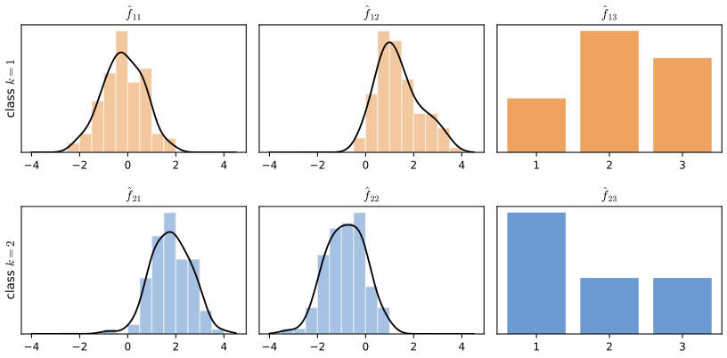
fig_4_10. Download: PDF · SVG| Naive Bayes on Default (recomputed) | True No | True Yes | Total |
|---|---|---|---|
| Table 4.8, threshold 0.5: predicted No | 9,615 | 241 | 9,856 |
| Table 4.8, threshold 0.5: predicted Yes | 52 | 92 | 144 |
| Table 4.9, threshold 0.2: predicted No | 9,320 | 128 | 9,448 |
| Table 4.9, threshold 0.2: predicted Yes | 347 | 205 | 552 |
Against LDA the results are mixed: at 0.5 naive Bayes has a slightly higher error (2.93% against 2.75%) but catches more defaulters (92 against 81); at 0.2 it catches 205 of 333 (61.6%, the book's "almost two-thirds") at an error of 4.75%. With \(n=10{,}000\) and so few predictors there is little variance for the independence assumption to save.
Deeper: Statistical Learning: Theory and Methods, Section 6.6.3 (naive Bayes with kernel density estimates, and Result 6.15: its log-odds are additive). See also: Foundations of Deep Learning, Result 5.13 (naive Bayes for binary features is linear, and its maximum likelihood fit is counting).
4.5 A Comparison of Classification Methods
4.5.1 An Analytical Comparison
pp. 158–161 With class \(K\) as baseline, each method classifies to the \(k\) that maximises the log-odds
\[ \log\Big(\frac{\Pr(Y=k\given X=x)}{\Pr(Y=K\given X=x)}\Big), \tag{4.31} \]and comparing the form of (4.31) across methods explains how they differ. For LDA,
\[ \begin{aligned}\log\Big(\frac{\Pr(Y=k\given X=x)}{\Pr(Y=K\given X=x)}\Big)&=\log\Big(\frac{\pi_kf_k(x)}{\pi_Kf_K(x)}\Big)=\log\Big(\frac{\pi_k}{\pi_K}\Big)-\tfrac12(x-\mu_k)^\T\Sigma^{-1}(x-\mu_k)+\tfrac12(x-\mu_K)^\T\Sigma^{-1}(x-\mu_K)\\&=\log\Big(\frac{\pi_k}{\pi_K}\Big)-\tfrac12(\mu_k+\mu_K)^\T\Sigma^{-1}(\mu_k-\mu_K)+x^\T\Sigma^{-1}(\mu_k-\mu_K)=a_k+\sum_{j=1}^pb_{kj}x_j,\end{aligned} \tag{4.32} \]with
\[ a_k=\log(\pi_k/\pi_K)-\tfrac12(\mu_k+\mu_K)^\T\Sigma^{-1}(\mu_k-\mu_K), \]and \(b_{kj}\) the \(j\)th component of \(\Sigma^{-1}(\mu_k-\mu_K)\). For QDA,
\[ \log\Big(\frac{\Pr(Y=k\given X=x)}{\Pr(Y=K\given X=x)}\Big)=a_k+\sum_{j=1}^pb_{kj}x_j+\sum_{j=1}^p\sum_{l=1}^pc_{kjl}x_jx_l, \tag{4.33} \]and for naive Bayes,
\[ \log\Big(\frac{\Pr(Y=k\given X=x)}{\Pr(Y=K\given X=x)}\Big)=\log\Big(\frac{\pi_k}{\pi_K}\Big)+\sum_{j=1}^p\log\Big(\frac{f_{kj}(x_j)}{f_{Kj}(x_j)}\Big)=a_k+\sum_{j=1}^pg_{kj}(x_j), \tag{4.34} \]with \(a_k=\log(\pi_k/\pi_K)\) and \(g_{kj}(x_j)=\log\{f_{kj}(x_j)/f_{Kj}(x_j)\}\): an additive model, the form of the generalised additive models of Chapter 7.
Filling the gap 4.8: the middle step of (4.32), and the coefficients of (4.33) (Exercises 10 and 11) pp. 158–159
(a) In (4.32) the quadratic terms \(x^\T\Sigma^{-1}x\) cancel and \[ -\tfrac12\mu_k^\T\Sigma^{-1}\mu_k+\tfrac12\mu_K^\T\Sigma^{-1}\mu_K=-\tfrac12(\mu_k+\mu_K)^\T\Sigma^{-1}(\mu_k-\mu_K). \]
(b) In (4.33),
\[ a_k=\log\frac{\pi_k}{\pi_K}-\tfrac12\log\frac{|\Sigma_k|}{|\Sigma_K|}-\tfrac12\big(\mu_k^\T\Sigma_k^{-1}\mu_k-\mu_K^\T\Sigma_K^{-1}\mu_K\big),\quad b_{kj}=\big[\Sigma_k^{-1}\mu_k-\Sigma_K^{-1}\mu_K\big]_j,\quad c_{kjl}=-\tfrac12\big[\Sigma_k^{-1}-\Sigma_K^{-1}\big]_{jl}. \](c) For \(p=1\), (4.32) has \(a_k=\log(\pi_k/\pi_K)-\frac{\mu_k^2-\mu_K^2}{2\sigma^2}\) and \(b_{k1}=\frac{\mu_k-\mu_K}{\sigma^2}\).
Derivation
(a) Expand both quadratic forms as in Filling the gap 4.5: \[ -\frac12x^\T\Sigma^{-1}x+x^\T\Sigma^{-1}\mu_k-\frac12\mu_k^\T\Sigma^{-1}\mu_k \] minus the same with \(K\). The first terms cancel, the middle ones give \(x^\T\Sigma^{-1}(\mu_k-\mu_K)\), and for the last ones, by symmetry of \(\Sigma^{-1}\), \[ (\mu_k+\mu_K)^\T\Sigma^{-1}(\mu_k-\mu_K)=\mu_k^\T\Sigma^{-1}\mu_k-\mu_K^\T\Sigma^{-1}\mu_K \] (the cross terms \(\mu_K^\T\Sigma^{-1}\mu_k-\mu_k^\T\Sigma^{-1}\mu_K\) cancel).
(b) Subtract the second line of (4.28) for class \(K\) from that for class \(k\): the \(x^\T(\cdot)x\) part is \[ -\frac12x^\T(\Sigma_k^{-1}-\Sigma_K^{-1})x=\sum_j\sum_lc_{kjl}x_jx_l \], the linear part is \(x^\T(\Sigma_k^{-1}\mu_k-\Sigma_K^{-1}\mu_K)\), and the rest is constant. Because the double sum runs over all ordered pairs \((j,l)\), each product \(x_jx_l\) with \(j\ne l\) appears twice, with total coefficient \(2c_{kjl}\). Both formulas were confirmed numerically on the Default data: the log-odds computed from the fitted LDA and QDA posteriors equal \(a_k+b_k^\T x\) and \(a_k+b_k^\T x+x^\T C_kx\) to \(10^{-8}\).
(c) Put \(p=1\), \(\Sigma=\sigma^2\) in (a): \[ \frac12(\mu_k+\mu_K)(\mu_k-\mu_K)/\sigma^2=(\mu_k^2-\mu_K^2)/(2\sigma^2) \].
Result 4.6 (how the methods are related) pp. 159–161
(a) LDA is the special case of QDA with all \(c_{kjl}=0\) (equal covariances). (b) Any classifier with linear log-odds, LDA included, is the special case of naive Bayes with \(g_{kj}(x_j)=b_{kj}x_j\). (c) Naive Bayes with normal margins \(\N(\mu_{kj},\sigma_j^2)\) whose variance does not depend on the class is LDA with a diagonal \(\Sigma\): \(g_{kj}(x_j)=b_{kj}x_j+\text{const}\) with \(b_{kj}=(\mu_{kj}-\mu_{Kj})/\sigma_j^2\). (d) Neither QDA nor naive Bayes contains the other: naive Bayes allows any functions \(g_{kj}\) but no products \(x_jx_l\); QDA allows products but only quadratic functions. (e) Multinomial logistic regression (4.12) has exactly the linear form of LDA; the two differ only in how the coefficients are estimated.
Proof and discussion
(a) and (d) are read off (4.32)–(4.34). (b) Statement (b) concerns the form of the rule: a linear function \(a_k+\sum_jb_{kj}x_j\) is a sum of functions of one variable each. It does not say that fitting naive Bayes to data gives the LDA fit, since naive Bayes estimates each \(g_{kj}\) from its own margins. (c) \[ \log\frac{f_{kj}(x_j)}{f_{Kj}(x_j)}=-\frac{(x_j-\mu_{kj})^2-(x_j-\mu_{Kj})^2}{2\sigma_j^2}=\frac{(\mu_{kj}-\mu_{Kj})x_j}{\sigma_j^2}-\frac{\mu_{kj}^2-\mu_{Kj}^2}{2\sigma_j^2} \]. If each class has its own variance \(\sigma_{kj}^2\), the \(x_j^2\) term survives and naive Bayes is QDA with diagonal covariance matrices (as in the lab).
(e) In LDA the coefficients \(a_k,b_k\) are functions of \(\hat\pi_k,\hat\mu_k,\hat\Sigma\), i.e. they maximise the joint likelihood of \((X,Y)\) under normality; logistic regression maximises the conditional likelihood of \(Y\) given \(X\) and assumes nothing about the distribution of \(X\). When the normal model is right, LDA uses more information and is more efficient (Efron 1975 found it needs roughly 30% to 50% fewer observations for the same accuracy in typical cases); when it is wrong (heavy tails, binary predictors, outliers), logistic regression is safer. On the Default data the two give almost the same ROC curve (AUC 0.9496 and 0.9495) and, on Smarket, identical predictions for 2005 (Section 4.7.3). ∎
pp. 160–161 K-nearest neighbours (Chapter 2) assigns \(x\) to the most common class among the \(K\) training points closest to it. It assumes nothing about the shape of the boundary, so it should beat LDA and logistic regression when the boundary is very non-linear, provided \(n\) is large and \(p\) small; it needs many observations per predictor (Exercise 4 shows why); with a non-linear boundary but moderate \(n\), QDA is often the better compromise; and it gives no coefficients, so it does not tell which predictors matter.
Deeper: Statistical Learning: Theory and Methods, Section 4.4.5 (Result 4.12: LDA as a plug-in logistic model, and what the marginal likelihood of \(X\) buys); Section 2.3.2 (nearest neighbours) and Section 2.5 (local methods in high dimensions).
4.5.2 An Empirical Comparison
pp. 161–164 Six two-class simulations with \(p=2\) quantitative predictors, 100 training sets each, test error on a large test set, for KNN with \(K=1\), KNN with \(K\) chosen by cross-validation (Chapter 5), LDA, logistic regression, naive Bayes (normal margins) and QDA. The book describes the scenarios in words only; the settings used here (listed in the code) follow those descriptions and the ranges of the book's axes:
- Scenario 1: 20 points per class, independent normal predictors with different means. LDA's model.
- Scenario 2: as 1, with correlation −0.5 within each class.
- Scenario 3: as 2, but bivariate \(t\) (here with 2 degrees of freedom) and 50 points per class: heavy tails.
- Scenario 4: normal, correlation 0.5 in one class and −0.5 in the other, so the Bayes boundary is quadratic (QDA's model).
- Scenario 5: independent normal predictors, responses drawn from a logistic model with a complicated non-linear function (here \(0.7\{3x_1+1.2x_2^2-1.2\) \(+\,1.5\sin(3x_2)+1.5\sin(2x_1x_2)\}\)).
- Scenario 6: normal with a different diagonal covariance in each class, only 6 points per class (naive Bayes' model).
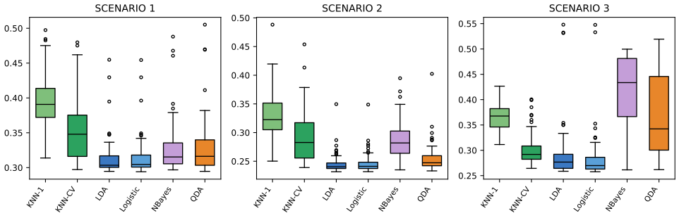
fig_4_11. Download: PDF · SVG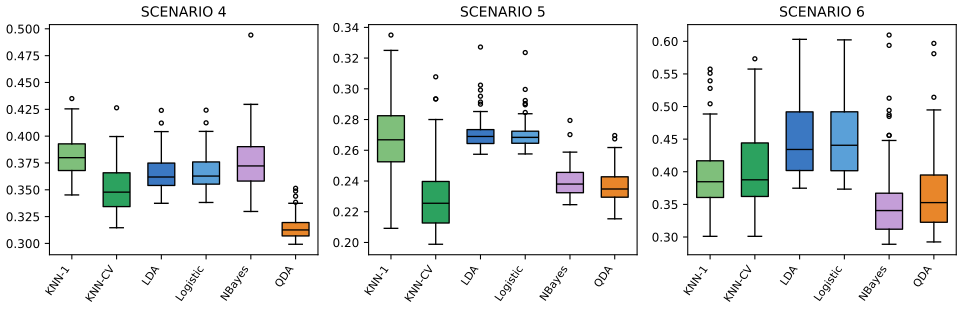
fig_4_12. Download: PDF · SVGThe conclusions are the book's, and the simulations here bear each of them out: LDA and logistic regression win when the boundary is linear (Scenarios 1–2), logistic regression is the more robust of the two under heavy tails (3), QDA wins for a quadratic boundary (4), the cross-validated KNN wins for a complicated boundary while KNN with \(K=1\) is as bad as the linear rules (5), and with very few observations naive Bayes' strong assumption pays (6). Naive Bayes loses whenever the predictors are correlated within the classes (2–4). No method dominates; the right amount of flexibility depends on the problem and must be chosen from the data (Chapter 5). Adding \(X^2\), \(X^3\) or products to logistic regression or LDA is another way to move between these extremes; LDA with all squares and products has the same form as QDA, with different estimates.
4.6 Generalized Linear Models
pp. 164–165 Some responses are neither quantitative in the usual sense nor qualitative: counts. The Bikeshare data record, for each of 8,645 hours in Washington, DC, the number of bike-share users bikers, with the month mnth, the hour hr (0–23), workingday (1 if neither weekend nor holiday), the normalised temperature temp and the weather weathersit (clear; misty or cloudy; light rain or snow; heavy rain or snow). Month, hour and weather are treated as qualitative.
4.6.1 Linear Regression on the Bikeshare Data
pp. 165–167 Least squares (Table 4.10, Figure 4.13) gives sensible-looking effects: cloudy weather costs 12.89 bikers an hour relative to clear weather, light rain or snow a further 53.60; use peaks in spring and autumn and at the commuting hours.
| Table 4.10 (recomputed) | Coefficient | Std. error | t-statistic | p-value |
|---|---|---|---|---|
| Intercept | 73.60 | 5.13 | 14.34 | 0.00 |
| workingday | 1.27 | 1.78 | 0.71 | 0.48 |
| temp | 157.21 | 10.26 | 15.32 | 0.00 |
| weathersit[cloudy/misty] | −12.89 | 1.96 | −6.56 | 0.00 |
| weathersit[light rain/snow] | −66.49 | 2.97 | −22.42 | 0.00 |
| weathersit[heavy rain/snow] | −109.75 | 76.67 | −1.43 | 0.15 |
Month and hour use the sum-to-zero coding (Filling the gap 4.11), so each of their coefficients is a deviation from the average month or hour; the intercept is then the fitted mean at clear weather, a non-working day and temperature 0, averaged over months and hours.
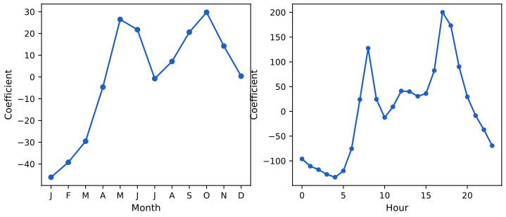
fig_4_13. Download: PDF · SVGBut 9.6% of the fitted values are negative (the smallest is −144), and the spread of the counts grows with their mean (Figure 4.14): between 1 and 4 AM in December–February in light rain or snow there are 5.05 users on average (standard deviation 3.73), between 7 and 10 AM in April–June in clear weather 243.59 (standard deviation 131.7). (These are the hours starting at 1, 2, 3 and at 7, 8, 9.) A linear model assumes constant variance and a continuous response. Logging the response removes the negative fits and most of the heteroscedasticity, but predictions and coefficients then refer to \(\E\log Y\), not \(\E Y\), and \(\log 0\) is undefined.
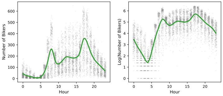
fig_4_14. Download: PDF · SVG4.6.2 Poisson Regression on the Bikeshare Data
pp. 167–170 A random variable \(Y\in\{0,1,2,\dots\}\) has the Poisson distribution with mean \(\lambda>0\) if
\[ \Pr(Y=k)=\frac{e^{-\lambda}\lambda^k}{k!}\quad\text{for }k=0,1,2,\dots \tag{4.35} \]Then \(\E(Y)=\Var(Y)=\lambda\): the larger the mean, the larger the variance. With \(\lambda=5\), \(\Pr(Y=0)=e^{-5}=0.0067\), \(\Pr(Y=1)=5e^{-5}=0.034\), \(\Pr(Y=2)=0.084\). Poisson regression lets the mean depend on the covariates through its logarithm,
\[ \log\big(\lambda(X_1,\dots,X_p)\big)=\beta_0+\beta_1X_1+\dots+\beta_pX_p, \tag{4.36} \]or equivalently
\[ \lambda(X_1,\dots,X_p)=e^{\beta_0+\beta_1X_1+\dots+\beta_pX_p}, \tag{4.37} \]which is positive whatever the coefficients. The coefficients are estimated by maximising the likelihood
\[ \ell(\beta_0,\beta_1,\dots,\beta_p)=\prod_{i=1}^n\frac{e^{-\lambda(x_i)}\lambda(x_i)^{y_i}}{y_i!},\qquad\lambda(x_i)=e^{\beta_0+\beta_1x_{i1}+\dots+\beta_px_{ip}}. \tag{4.38} \]Filling the gap 4.9: the Poisson distribution and the Poisson likelihood pp. 167–168
(a) The probabilities (4.35) sum to one and \(\E Y=\Var Y=\lambda\). (b) With \(\eta_i=x_i^\T\beta\), the log-likelihood is \(L(\beta)=\sum_i\{y_i\eta_i-e^{\eta_i}-\log y_i!\}\), with score \(\bX^\T(\by-\boldsymbol\lambda)\) and Hessian \(-\bX^\T\diag(\lambda_i)\bX\): strictly concave, maximised by Newton's method exactly as in Algorithm 4.1 with weights \(\lambda_i\) instead of \(p_i(1-p_i)\). (c) The score equations say that the fitted counts add up to the observed counts within every column of \(\bX\): overall (intercept), and within each month and each hour when these are coded by indicators or sum-to-zero contrasts.
Derivation
(a) \(\sum_k\lambda^k/k!=e^\lambda\) (the exponential series), so \(\sum_k\Pr(Y=k)=1\). \[ \E Y=\sum_{k\ge1}k\frac{e^{-\lambda}\lambda^k}{k!}=\lambda\sum_{k\ge1}\frac{e^{-\lambda}\lambda^{k-1}}{(k-1)!}=\lambda \]. Similarly \(\E\{Y(Y-1)\}=\lambda^2\), so \(\Var Y=\lambda^2+\lambda-\lambda^2=\lambda\).
(b) \(\log\{e^{-\lambda}\lambda^y/y!\}=y\log\lambda-\lambda-\log y!\) and \(\log\lambda_i=\eta_i\). Then \(\partial L/\partial\beta=\sum_i(y_i-e^{\eta_i})x_i\) and \[ \partial^2L/\partial\beta\partial\beta^\T=-\sum_ie^{\eta_i}x_ix_i^\T \], negative definite for full-rank \(\bX\). The Newton step is \[ \beta\leftarrow\beta+(\bX^\T\bW\bX)^{-1}\bX^\T(\by-\boldsymbol\lambda) \] with \(\bW=\diag(\lambda_i)\); on the Bikeshare data it converges in 9 steps from \(\beta_0=\log\bar y\).
(c) \(\bX^\T(\by-\hat{\boldsymbol\lambda})=0\), row by row. The indicator of a month lies in the column space of the intercept and the month contrasts, so \[ \sum_{i\in\text{month}}\hat\lambda_i=\sum_{i\in\text{month}}y_i \]; the same holds for each hour. Confirmed numerically for all 24 hours. In particular a model with hour only fits the 24 hourly means exactly, for least squares and for Poisson regression alike.
| Table 4.11 (recomputed) | Coefficient | Std. error | z-statistic | p-value |
|---|---|---|---|---|
| Intercept | 4.12 | 0.01 | 683.96 | 0.00 |
| workingday | 0.01 | 0.00 | 7.50 | 0.00 |
| temp | 0.79 | 0.01 | 68.43 | 0.00 |
| weathersit[cloudy/misty] | −0.08 | 0.00 | −34.53 | 0.00 |
| weathersit[light rain/snow] | −0.58 | 0.00 | −141.90 | 0.00 |
| weathersit[heavy rain/snow] | −0.93 | 0.17 | −5.55 | 0.00 |
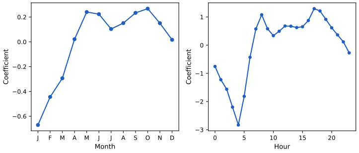
fig_4_15. Download: PDF · SVGResult 4.7 (reading a Poisson regression) pp. 168–170
(a) Interpretation: increasing \(X_j\) by one unit, the others fixed, multiplies the mean by \(e^{\beta_j}\). Cloudy instead of clear weather multiplies the mean number of bikers by \(e^{-0.0752}=0.928\) (the book rounds the coefficient to −0.08 and reports 0.923); light rain instead of cloudy multiplies it by \(e^{-0.5758+0.0752}=0.606\). (b) Mean and variance: the model implies \(\Var(Y\given x)=\E(Y\given x)\), so it accommodates variance that grows with the mean, where least squares assumes it constant. (c) Fitted values \(e^{x^\T\hat\beta}\) are always positive (the smallest here is 1.20), against 9.6% negative fits for least squares. (d) Overdispersion: the data are far more variable than the Poisson model allows (Pearson dispersion \[ \hat\phi=\sum_i(y_i-\hat\lambda_i)^2/\hat\lambda_i/(n-p-1)=25.6 \]), so the standard errors of Table 4.11 are too small by a factor of about \(\sqrt{25.6}\approx5\), and the \(z\) statistics too large by the same factor (the book's footnote 5).
Proof and a remark on workingday
(a) By (4.37), \(\lambda(x+e_j)/\lambda(x)=e^{\beta_j}\). (b) is the property \(\E Y=\Var Y\) of (4.35). (c) is the exponential. (d) If \(\Var(Y\given x)=\phi\,\E(Y\given x)\) instead, the maximum likelihood estimates are unchanged (the score equations do not involve \(\phi\)), but their covariance is \(\phi(\bX^\T\bW\bX)^{-1}\); the Pearson statistic estimates \(\phi\). This "quasi-Poisson" correction is one of the methods the book alludes to; the negative binomial model is another. The book notes that workingday is significant for Poisson regression (\(z=7.5\)) but not for least squares (\(t=0.71\)); after the overdispersion correction its \(z\) is about \(7.5/5.06=1.5\), no longer significant, so this difference is largely an artefact of the Poisson variance assumption. ∎
4.6.3 Generalized Linear Models in Greater Generality
pp. 170–171 Linear, logistic and Poisson regression share two features: given the predictors, \(Y\) has a distribution from a known family (normal, Bernoulli, Poisson), and a transformation of its mean is linear in the predictors:
\[ \E(Y\given X_1,\dots,X_p)=\beta_0+\beta_1X_1+\dots+\beta_pX_p, \tag{4.39} \] \[ \E(Y\given X_1,\dots,X_p)=\Pr(Y=1\given X_1,\dots,X_p)=\frac{e^{\beta_0+\beta_1X_1+\dots+\beta_pX_p}}{1+e^{\beta_0+\beta_1X_1+\dots+\beta_pX_p}}, \tag{4.40} \] \[ \E(Y\given X_1,\dots,X_p)=\lambda(X_1,\dots,X_p)=e^{\beta_0+\beta_1X_1+\dots+\beta_pX_p}, \tag{4.41} \]that is, with a link function \(\eta\),
\[ \eta\big(\E(Y\given X_1,\dots,X_p)\big)=\beta_0+\beta_1X_1+\dots+\beta_pX_p, \tag{4.42} \]with \(\eta(\mu)=\mu\), \(\log\{\mu/(1-\mu)\}\) and \(\log\mu\) respectively.
Definition 4.3 (generalised linear model) pp. 170–171
A generalised linear model (GLM) has three parts: (i) the response, given \(x\), has a distribution in an exponential family, \(f(y;\theta,\phi)=\exp\{(y\theta-b(\theta))/\phi+c(y,\phi)\}\), with mean \(\mu=b'(\theta)\) and variance \(\phi\,b''(\theta)\); (ii) a linear predictor \(x^\T\beta\); (iii) a link \(\eta\) with \(\eta(\mu)=x^\T\beta\). The link that makes \(\theta=x^\T\beta\) is the canonical link.
Filling the gap 4.10: the three models as exponential families p. 171
Normal: \(\theta=\mu\), \(b(\theta)=\theta^2/2\), \(\phi=\sigma^2\), variance \(\sigma^2\), canonical link the identity. Bernoulli: \(\theta=\log\{\mu/(1-\mu)\}\), \(b(\theta)=\log(1+e^\theta)\), \(\phi=1\), variance \(\mu(1-\mu)\), canonical link the logit. Poisson: \(\theta=\log\mu\), \(b(\theta)=e^\theta\), \(\phi=1\), variance \(\mu\), canonical link the log. With the canonical link the score is always \(\bX^\T(\by-\boldsymbol\mu)/\phi\), so the fitted means reproduce the observed totals of every column of \(\bX\), and Newton's method is the same weighted least squares iteration with weights \(\Var(Y_i)/\phi\).
Derivation
Write each density as \(\exp\{y\theta-b(\theta)+c(y)\}\): normal (\(\sigma=1\)): \(-\frac12(y-\mu)^2=y\mu-\frac{\mu^2}{2}-\frac{y^2}{2}\); Bernoulli: \(\mu^y(1-\mu)^{1-y}\) \(=\exp\{y\log\frac{\mu}{1-\mu}+\log(1-\mu)\}\) and \(-\log(1-\mu)=\log(1+e^\theta)\); Poisson: \(\exp\{y\log\mu-\mu-\log y!\}\). Then \(b'(\theta)\) is \(\theta\), \(e^\theta/(1+e^\theta)\) and \(e^\theta\), the three means, and \(b''(\theta)\) is 1, \(\mu(1-\mu)\) and \(\mu\), the three variances. With \(\theta_i=x_i^\T\beta\), \(\partial\log f/\partial\beta=\{y_i-b'(\theta_i)\}x_i/\phi\) and the Hessian is \(-\sum_ib''(\theta_i)x_ix_i^\T/\phi\), which gives the score and the weights. Gamma and negative binomial regression, the book's other examples, fit the same pattern (the Gamma family with variance \(\phi\mu^2\)).
See also (companion courses): Statistical Methods for Modern Biology, Section 8.8 (generalised linear models for counts, in R, and the negative binomial model for overdispersed counts in Section 8.4.1); Foundations of Deep Learning, Section 5.4.6 and Result 5.20 (canonical links give the error-times-feature gradient).
4.7 Lab: Classification Methods in R and Python
pp. 171–189 The lab follows the steps of the R lab of James et al. (2021) and the Python lab of James et al. (2023): logistic regression, LDA, QDA, naive Bayes and KNN on the stock market data, KNN and logistic regression on the Caravan insurance data, and linear and Poisson regression on Bikeshare. The code is written for this course.
The files. code/ch04_lab.R (run with Rscript ch04_lab.R from the code folder; it needs the CRAN packages ISLR2, MASS, e1071 and class) and code/ch04_lab.py (run with python3 ch04_lab.py; it needs numpy, pandas, matplotlib, statsmodels and scikit-learn, but not the book's helper package). The code below is copied from these files, R on the left and Python on the right. Both scripts print every result as a line label: values with the same labels, through two tiny helpers show() and show_table() defined at the top of each file, so the two outputs can be compared line by line. Every number below is the same in the two languages unless an orange note says otherwise.
4.7.1 The Stock Market Data
Smarket holds 1,250 trading days of the S&P 500 (2001–2005): the percentage returns of the five previous days (Lag1–Lag5), the volume of the previous day in billions of shares, today's return and its direction (602 Down, 648 Up). The lags are almost uncorrelated with today's return; the only sizeable correlation is between year and volume, which grew over the five years.
R
cors <- cor(Smarket[, names(Smarket) != "Direction"])
show("cor(Year, Volume)", cors["Year", "Volume"], 3)
lags <- c("Lag1", "Lag2", "Lag3", "Lag4", "Lag5", "Today")
lag.cor <- cors[lags, lags]
show("largest |cor| among Lag1-Lag5 and Today", max(abs(lag.cor[upper.tri(lag.cor)])), 3)
png(file.path(img_dir, "lab4-r-volume.png"), width = 640, height = 380, res = 110)
plot(Smarket$Volume, pch = 20, cex = 0.5, col = "grey30", xlab = "Day (2001-2005)", ylab = "Volume")
invisible(dev.off())
Python
cors = Smarket.drop(columns="Direction").corr()
show("cor(Year, Volume)", cors.loc["Year", "Volume"], 3)
lags = ["Lag1", "Lag2", "Lag3", "Lag4", "Lag5", "Today"]
lag_cor = cors.loc[lags, lags].values
show("largest |cor| among Lag1-Lag5 and Today", np.max(np.abs(lag_cor[np.triu_indices(6, 1)])), 3)
fig, ax = common.plt.subplots(figsize=(6.4, 3.4))
ax.plot(Smarket.Volume.values, ".", ms=2.5, color="0.3")
ax.set_xlabel("Day (2001-2005)")
ax.set_ylabel("Volume")
common.savefig(fig, 4, "lab4-py-volume")
cor(Year, Volume): 0.539
largest |cor| among Lag1-Lag5 and Today: 0.035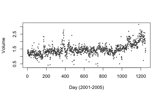
plot(Smarket$Volume).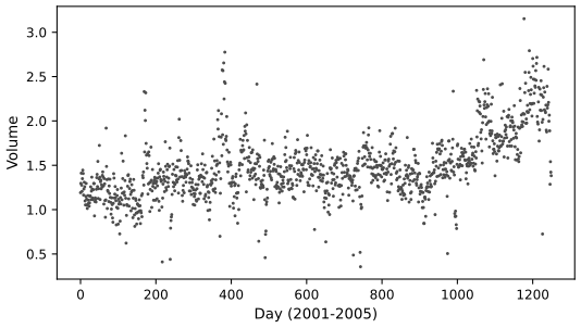
4.7.2 Logistic Regression
Logistic regression of Direction on the five lags and volume, on all 1,250 days. R's glm() takes the second level of the factor, Up, as 1; the Python code makes the 0/1 response explicitly.
R
glm.fits <- glm(Direction ~ Lag1 + Lag2 + Lag3 + Lag4 + Lag5 + Volume,
                data = Smarket, family = binomial)
print(round(summary(glm.fits)$coef, 4))
show("residual deviance", deviance(glm.fits), 2)
glm.probs <- predict(glm.fits, type = "response")      # Pr(Up | x): R codes Up as 1
show("first five fitted probabilities", glm.probs[1:5])
glm.pred <- ifelse(glm.probs > 0.5, "Up", "Down")
show_table("training confusion (all 1250 days)", table(glm.pred, Smarket$Direction))
show("training accuracy", mean(glm.pred == Smarket$Direction))
Python
y = (Smarket.Direction == "Up").astype(int)               # 1 = Up, as in R
X = sm.add_constant(Smarket[["Lag1", "Lag2", "Lag3", "Lag4", "Lag5", "Volume"]])
results = sm.GLM(y, X, family=sm.families.Binomial()).fit()
print(pd.DataFrame({"coef": results.params, "std err": results.bse, "z": results.tvalues,
                    "P>|z|": results.pvalues}).round(4))
show("residual deviance", results.deviance, 2)
probs = results.predict()
show("first five fitted probabilities", probs[:5])
labels = np.where(probs > 0.5, "Up", "Down")
show_table("training confusion (all 1250 days)", labels, Smarket.Direction)
show("training accuracy", np.mean(labels == Smarket.Direction))
coef std err z P>|z|
const -0.1260 0.2407 -0.5234 0.6007
Lag1 -0.0731 0.0502 -1.4566 0.1452
Lag2 -0.0423 0.0501 -0.8446 0.3984
Lag3 0.0111 0.0499 0.2220 0.8243
Lag4 0.0094 0.0500 0.1873 0.8514
Lag5 0.0103 0.0495 0.2083 0.8350
Volume 0.1354 0.1584 0.8553 0.3924
residual deviance: 1727.58
first five fitted probabilities: 0.5071 0.4815 0.4811 0.5152 0.5108
training confusion (rows predicted Down, Up; columns true Down, Up): 145 141 / 457 507
training accuracy: 0.5216No predictor is significant (the smallest p-value, 0.145, is for Lag1), and the training accuracy of 52.2% is barely above the 51.8% of always saying Up. Training accuracy is also optimistic, so the next step trains on 2001–2004 and tests on the 252 days of 2005.
R
train <- Smarket$Year < 2005
Smarket.2005 <- Smarket[!train, ]
Direction.2005 <- Smarket$Direction[!train]
show("test days in 2005", nrow(Smarket.2005), 0)

glm.fits <- glm(Direction ~ Lag1 + Lag2 + Lag3 + Lag4 + Lag5 + Volume,
                data = Smarket, family = binomial, subset = train)
glm.probs <- predict(glm.fits, Smarket.2005, type = "response")
glm.pred <- ifelse(glm.probs > 0.5, "Up", "Down")
show_table("2005 confusion, six predictors", table(glm.pred, Direction.2005))
show("2005 accuracy, six predictors", mean(glm.pred == Direction.2005))

glm.fits <- glm(Direction ~ Lag1 + Lag2, data = Smarket, family = binomial, subset = train)
glm.probs <- predict(glm.fits, Smarket.2005, type = "response")
glm.pred <- ifelse(glm.probs > 0.5, "Up", "Down")
show_table("2005 confusion, Lag1 + Lag2", table(glm.pred, Direction.2005))
show("2005 accuracy, Lag1 + Lag2", mean(glm.pred == Direction.2005))
show("precision on predicted Up days", mean(Direction.2005[glm.pred == "Up"] == "Up"))
show("always-Up accuracy in 2005", mean(Direction.2005 == "Up"))
show("Pr(Up) at (1.2, 1.1) and (1.5, -0.8)",
     predict(glm.fits, newdata = data.frame(Lag1 = c(1.2, 1.5), Lag2 = c(1.1, -0.8)), type = "response"))
Python
train = (Smarket.Year < 2005).values
L_train, L_test = Smarket.Direction[train], Smarket.Direction[~train]
show("test days in 2005", np.sum(~train), 0)

results = sm.GLM(y[train], X[train], family=sm.families.Binomial()).fit()
probs = results.predict(X[~train])
labels = np.where(probs > 0.5, "Up", "Down")
show_table("2005 confusion, six predictors", labels, L_test)
show("2005 accuracy, six predictors", np.mean(labels == L_test))

X2 = sm.add_constant(Smarket[["Lag1", "Lag2"]])
results = sm.GLM(y[train], X2[train], family=sm.families.Binomial()).fit()
probs = results.predict(X2[~train])
labels = np.where(probs > 0.5, "Up", "Down")
show_table("2005 confusion, Lag1 + Lag2", labels, L_test)
show("2005 accuracy, Lag1 + Lag2", np.mean(labels == L_test))
show("precision on predicted Up days", np.mean(L_test[labels == "Up"] == "Up"))
show("always-Up accuracy in 2005", np.mean(L_test == "Up"))
newX = sm.add_constant(pd.DataFrame({"Lag1": [1.2, 1.5], "Lag2": [1.1, -0.8]}), has_constant="add")
show("Pr(Up) at (1.2, 1.1) and (1.5, -0.8)", results.predict(newX))
2005 confusion, six predictors: 77 97 / 34 44
2005 accuracy, six predictors: 0.4802
2005 confusion, Lag1 + Lag2: 35 35 / 76 106
2005 accuracy, Lag1 + Lag2: 0.5595
precision on predicted Up days: 0.5824
always-Up accuracy in 2005: 0.5595
Pr(Up) at (1.2, 1.1) and (1.5, -0.8): 0.4791 0.4961With six predictors the test accuracy is 48%, worse than a coin. Dropping the four useless predictors lowers the variance and raises it to 56%, which is exactly the accuracy of always predicting Up in 2005; on the days the model predicts Up it is right 58% of the time. The two new days get probabilities just below one half.
4.7.3 Linear Discriminant Analysis
R
lda.fit <- lda(Direction ~ Lag1 + Lag2, data = Smarket, subset = train)
show("priors (Down, Up)", lda.fit$prior)
show("group means Down (Lag1, Lag2)", lda.fit$means["Down", ])
show("group means Up (Lag1, Lag2)", lda.fit$means["Up", ])
show("LD1 coefficients (Lag1, Lag2)", lda.fit$scaling[, 1])
lda.pred <- predict(lda.fit, Smarket.2005)
show_table("2005 confusion, LDA", table(lda.pred$class, Direction.2005))
show("2005 accuracy, LDA", mean(lda.pred$class == Direction.2005))
show("days with Pr(Down) >= 0.5 and < 0.5",
     c(sum(lda.pred$posterior[, "Down"] >= 0.5), sum(lda.pred$posterior[, "Down"] < 0.5)), 0)
show("days with Pr(Down) > 0.9", sum(lda.pred$posterior[, "Down"] > 0.9), 0)
show("largest Pr(Down) in 2005", max(lda.pred$posterior[, "Down"]))
Python
X_train, X_test = Smarket.loc[train, ["Lag1", "Lag2"]], Smarket.loc[~train, ["Lag1", "Lag2"]]
lda = LDA(store_covariance=True).fit(X_train, L_train)     # classes_ = ['Down', 'Up']
show("priors (Down, Up)", lda.priors_)
show("group means Down (Lag1, Lag2)", lda.means_[0])
show("group means Up (Lag1, Lag2)", lda.means_[1])
show("LD1 coefficients (Lag1, Lag2)", lda.scalings_[:, 0])
lda_pred = lda.predict(X_test)
show_table("2005 confusion, LDA", lda_pred, L_test)
show("2005 accuracy, LDA", np.mean(lda_pred == L_test))
lda_prob = lda.predict_proba(X_test)
show("days with Pr(Down) >= 0.5 and < 0.5", [np.sum(lda_prob[:, 0] >= 0.5), np.sum(lda_prob[:, 0] < 0.5)], 0)
show("days with Pr(Down) > 0.9", np.sum(lda_prob[:, 0] > 0.9), 0)
show("largest Pr(Down) in 2005", lda_prob[:, 0].max())
priors (Down, Up): 0.4920 0.5080
group means Down (Lag1, Lag2): 0.0428 0.0339
group means Up (Lag1, Lag2): -0.0395 -0.0313
LD1 coefficients (Lag1, Lag2): -0.6420 -0.5135
2005 confusion, LDA: 35 35 / 76 106
2005 accuracy, LDA: 0.5595
days with Pr(Down) >= 0.5 and < 0.5: 70 182
days with Pr(Down) > 0.9: 0
largest Pr(Down) in 2005: 0.5202Down days tend to follow small gains and Up days small losses. The "coefficients of linear discriminants" are the direction \(\hat\Sigma^{-1}(\hat\mu_{\rm Up}-\hat\mu_{\rm Down})\), scaled to have within-class variance 1: a day with large \(-0.642\,\text{Lag1}-0.514\,\text{Lag2}\) is classified Up. LDA's predictions for 2005 are identical to those of logistic regression, as Result 4.6(e) leads one to expect, and its posterior probabilities never stray far from 1/2 (largest probability of a fall: 52.02%).
lda.classes_ (alphabetical: Down, Up), so predict_proba(...)[:, 0] is the probability of Down, as R's posterior[, "Down"].4.7.4 Quadratic Discriminant Analysis
R
qda.fit <- qda(Direction ~ Lag1 + Lag2, data = Smarket, subset = train)
show("QDA covariance of class Down",
     as.numeric(cov(Smarket[train & Smarket$Direction == "Down", c("Lag1", "Lag2")])))
qda.class <- predict(qda.fit, Smarket.2005)$class
show_table("2005 confusion, QDA", table(qda.class, Direction.2005))
show("2005 accuracy, QDA", mean(qda.class == Direction.2005))
Python
qda = QDA(store_covariance=True).fit(X_train, L_train)
show("QDA covariance of class Down", qda.covariance_[0].ravel())
qda_pred = qda.predict(X_test)
show_table("2005 confusion, QDA", qda_pred, L_test)
show("2005 accuracy, QDA", np.mean(qda_pred == L_test))
QDA covariance of class Down: 1.5066 -0.0392 -0.0392 1.5356
2005 confusion, QDA: 30 20 / 81 121
2005 accuracy, QDA: 0.5992QDA is right on 60% of the days of 2005. That is a single year of 252 days; a binomial standard error of about \(\sqrt{0.6\times0.4/252}=0.031\) means it is two standard errors above 0.54 but only 1.3 above the 56% of always saying Up, so, as the book says, it should be tested on more data before anyone trades on it.
4.7.5 Naive Bayes
R
nb.fit <- naiveBayes(Direction ~ Lag1 + Lag2, data = Smarket, subset = train)
show("NB mean and sd of Lag1 in class Down", nb.fit$tables$Lag1["Down", ])
x.down <- Smarket$Lag1[train & Smarket$Direction == "Down"]
show("by hand: mean, sd (divisor n - 1)", c(mean(x.down), sd(x.down)))
nb.class <- predict(nb.fit, Smarket.2005)
show_table("2005 confusion, naive Bayes", table(nb.class, Direction.2005))
show("2005 accuracy, naive Bayes", mean(nb.class == Direction.2005))
nb.preds <- predict(nb.fit, Smarket.2005, type = "raw")
show("first three Pr(Up), naive Bayes", nb.preds[1:3, "Up"])
Python
NB = GaussianNB().fit(X_train, L_train)
show("NB mean and sd of Lag1 in class Down", [NB.theta_[0, 0], np.sqrt(NB.var_[0, 0])])
x_down = X_train.Lag1[L_train == "Down"]
show("by hand: mean, sd (divisor n)", [x_down.mean(), x_down.std(ddof=0)])
nb_pred = NB.predict(X_test)
show_table("2005 confusion, naive Bayes", nb_pred, L_test)
show("2005 accuracy, naive Bayes", np.mean(nb_pred == L_test))
show("first three Pr(Up), naive Bayes", NB.predict_proba(X_test)[:3, 1])
# GaussianNB divides by n; R's naiveBayes() divides by n - 1. Rescaling the variances reproduces R.
n_k = np.array([np.sum(L_train == c) for c in NB.classes_])
NB.var_ = NB.var_ * (n_k / (n_k - 1))[:, None]
nb_pred_r = NB.predict(X_test)
show("2005 accuracy, naive Bayes with divisor n - 1", np.mean(nb_pred_r == L_test))
R: NB mean and sd of Lag1 in class Down: 0.0428 1.2274 Python: 0.0428 1.2262
R: 2005 confusion, naive Bayes: 28 20 / 83 121 Python: 29 20 / 82 121
R: 2005 accuracy, naive Bayes: 0.5913 Python: 0.5952
first three Pr(Up), naive Bayes: 0.5127 0.5238 0.5347 (both)
Python: 2005 accuracy, naive Bayes with divisor n - 1: 0.5913naiveBayes() estimates each class standard deviation with divisor \(n_k-1\), scikit-learn's GaussianNB with divisor \(n_k\) (the Python edition's footnote 6). The difference of 0.1% in the standard deviations moves one day of 2005 from Up to Down, so the accuracies are 0.5913 (R, the 2021 book) and 0.5952 (Python, the 2023 book's 29/20/82/121). Rescaling GaussianNB's variances by \(n_k/(n_k-1)\), as in the last lines of the Python code, gives R's result exactly.4.7.6 K-Nearest Neighbors
KNN has no fitting step: R's knn() takes the training inputs, the test inputs, the training labels and \(K\) in one call; scikit-learn's KNeighborsClassifier is fitted (stores the data) and then predicts.
R
train.X <- cbind(Smarket$Lag1, Smarket$Lag2)[train, ]
test.X <- cbind(Smarket$Lag1, Smarket$Lag2)[!train, ]
train.Direction <- Smarket$Direction[train]
set.seed(1)                       # knn() breaks ties at random
knn.pred <- knn(train.X, test.X, train.Direction, k = 1)
show_table("2005 confusion, KNN K = 1", table(knn.pred, Direction.2005))
show("2005 accuracy, KNN K = 1", mean(knn.pred == Direction.2005))
knn.pred <- knn(train.X, test.X, train.Direction, k = 3)
show("2005 accuracy, KNN K = 3", mean(knn.pred == Direction.2005))
Python
knn1 = KNeighborsClassifier(n_neighbors=1).fit(X_train, L_train)
knn1_pred = knn1.predict(X_test)
show_table("2005 confusion, KNN K = 1", knn1_pred, L_test)
show("2005 accuracy, KNN K = 1", np.mean(knn1_pred == L_test))
knn3 = KNeighborsClassifier(n_neighbors=3).fit(X_train, L_train)
show("2005 accuracy, KNN K = 3", np.mean(knn3.predict(X_test) == L_test))
2005 confusion, KNN K = 1: 43 58 / 68 83 (both)
2005 accuracy, KNN K = 1: 0.5000 (both)
2005 accuracy, KNN K = 3: 0.5357 (R) 0.5317 (Python)knn() includes all of them in the vote and breaks tied votes at random (hence set.seed(1)); scikit-learn keeps exactly \(K\) neighbours, chosen by their order in the training data, and breaks tied votes in favour of the first class. Lag1 and Lag2 are recorded to three decimals, so ties occur, and with \(K=3\) one day of 2005 is classified differently: 0.536 in the 2021 book and in R, 0.532 in the 2023 book and in Python.The Caravan data. 5,822 customers, 85 demographic predictors, and whether they bought caravan insurance (348, i.e. 5.98%). KNN depends on distances, so predictors on large scales would dominate (a difference of \$1,000 in salary would outweigh 50 years of age); all predictors are standardised first. The R edition uses the first 1,000 customers as the test set, which both scripts reproduce here.
R
standardized.X <- scale(Caravan[, -86])
show("variance of columns 1 and 2 before / after scaling",
     c(var(Caravan[, 1]), var(Caravan[, 2]), var(standardized.X[, 1]), var(standardized.X[, 2])))
test <- 1:1000                    # the first 1,000 customers form the test set
train.X <- standardized.X[-test, ]
test.X <- standardized.X[test, ]
train.Y <- Caravan$Purchase[-test]
test.Y <- Caravan$Purchase[test]
set.seed(1)
for (k in c(1, 3, 5)) {
  knn.pred <- knn(train.X, test.X, train.Y, k = k)
  tab <- table(knn.pred, test.Y)
  show(sprintf("Caravan KNN K = %d: error, predicted Yes, correct Yes, success rate", k),
       c(mean(knn.pred != test.Y), sum(tab["Yes", ]), tab["Yes", "Yes"], tab["Yes", "Yes"] / sum(tab["Yes", ])))
}
show("Caravan null error (always No)", mean(test.Y != "No"))
Python
features = Caravan.drop(columns="Purchase")
X_std = (features - features.mean()) / features.std()       # divisor n - 1, as R's scale()
show("variance of columns 1 and 2 before / after scaling",
     [features.iloc[:, 0].var(), features.iloc[:, 1].var(), X_std.iloc[:, 0].var(), X_std.iloc[:, 1].var()])


def caravan_knn(X_tr, X_te, y_tr, y_te, label):
    for k in (1, 3, 5):
        pred = KNeighborsClassifier(n_neighbors=k).fit(X_tr, y_tr).predict(X_te)
        yes = pred == "Yes"
        hit = np.sum(yes & (y_te == "Yes"))
        show("%s KNN K = %d: error, predicted Yes, correct Yes, success rate" % (label, k),
             [np.mean(pred != y_te), yes.sum(), hit, hit / max(yes.sum(), 1)])


# (a) the R edition's split: the first 1,000 customers are the test set
test = np.arange(len(Caravan)) < 1000
X_tr, X_te, y_tr, y_te = X_std[~test], X_std[test], Purchase[~test].values, Purchase[test].values
caravan_knn(X_tr, X_te, y_tr, y_te, "Caravan")
show("Caravan null error (always No)", np.mean(y_te != "No"))
variance of columns 1 and 2 before / after scaling: 165.0378 0.1647 1.0000 1.0000
Caravan KNN K = 1: error, predicted Yes, correct Yes, success rate: 0.1180 77 9 0.1169 (both)
Caravan KNN K = 3: ... R: 0.0750 26 5 0.1923 Python: 0.0740 25 5 0.2000
Caravan KNN K = 5: error, predicted Yes, correct Yes, success rate: 0.0660 15 4 0.2667 (both)
Caravan null error (always No): 0.0590The overall error (11.8% for \(K=1\)) is worse than the 5.9% of predicting "No" for everyone, but that is not the relevant measure: a salesperson visiting the customers predicted to buy succeeds 11.7% of the time with \(K=1\), 19% with \(K=3\) and 26.7% with \(K=5\), against 6% for random visits. The positive predictive value of Definition 4.2 is the quantity that matters here.
R
glm.fits <- suppressWarnings(glm(Purchase ~ ., data = Caravan, family = binomial, subset = -test))
glm.probs <- predict(glm.fits, Caravan[test, ], type = "response")
for (cut in c(0.5, 0.25)) {
  glm.pred <- factor(ifelse(glm.probs > cut, "Yes", "No"), levels = c("No", "Yes"))
  tab <- table(glm.pred, test.Y)
  show(sprintf("Caravan logistic, threshold %.2f: predicted Yes, correct Yes", cut),
       c(sum(tab["Yes", ]), tab["Yes", "Yes"]), 0)
}
Python
yb = (Purchase == "Yes").astype(int)
with warnings.catch_warnings():
    warnings.simplefilter("ignore")                         # some fitted probabilities are 0 or 1
    logit = sm.GLM(yb[~test], sm.add_constant(features[~test]), family=sm.families.Binomial()).fit()
glm_probs = logit.predict(sm.add_constant(features[test]))
for cut in (0.5, 0.25):
    yes = glm_probs.values > cut
    show("Caravan logistic, threshold %.2f: predicted Yes, correct Yes" % cut,
         [yes.sum(), np.sum(yes & (y_te == "Yes"))], 0)
Caravan logistic, threshold 0.50: predicted Yes, correct Yes: 7 0 (both)
Caravan logistic, threshold 0.25: predicted Yes, correct Yes: 33 11 (both)With the threshold 0.5, logistic regression flags 7 customers, none of whom buys; with 0.25 it flags 33, and 11 of them (33%) buy, more than five times the base rate. Both languages print a warning that some fitted probabilities are numerically 0 or 1 (Result 4.1, the remark on separation); the coefficients of a few rare predictors are large, but the predictions are usable.
The Python edition draws its 1,000 test customers at random instead (train_test_split with random_state=0) and standardises with divisor \(n\). The Python script runs that split too:
Python
scaled = pd.DataFrame(StandardScaler().fit_transform(features), columns=features.columns)
Xa, Xb, ya, yb2 = train_test_split(scaled, Purchase, test_size=1000, random_state=0)
caravan_knn(Xa, Xb, ya.values, yb2.values, "Caravan (random split)")
show("Caravan (random split) null error", np.mean(yb2 != "No"))
Caravan (random split) KNN K = 1: 0.1110 62 9 0.1452
Caravan (random split) KNN K = 3: 0.0810 20 3 0.1500
Caravan (random split) KNN K = 5: 0.0720 7 1 0.1429
Caravan (random split) null error: 0.0670LogisticRegression(C=1e10), a barely penalised fit; statsmodels' unpenalised GLM, used here, reproduces R's glm().4.7.7 Poisson Regression
Least squares on Bikeshare, first with the default coding of the factors, then with the sum-to-zero coding of Section 4.6.
R
mod.lm <- lm(bikers ~ mnth + hr + workingday + temp + weathersit, data = Bikeshare)
show("lm (treatment coding): intercept, mnthFeb, mnthMarch", coef(mod.lm)[1:3], 3)
contrasts(Bikeshare$hr) <- contr.sum(24)
contrasts(Bikeshare$mnth) <- contr.sum(12)
mod.lm2 <- lm(bikers ~ mnth + hr + workingday + temp + weathersit, data = Bikeshare)
show("lm (sum coding): intercept, Jan, Feb", coef(mod.lm2)[1:3], 3)
show("max |difference| of fitted values between the codings",
     max(abs(fitted(mod.lm) - fitted(mod.lm2))), 10)
coef.months <- c(coef(mod.lm2)[2:12], -sum(coef(mod.lm2)[2:12]))
coef.hours <- c(coef(mod.lm2)[13:35], -sum(coef(mod.lm2)[13:35]))
show("lm December and hour-23 effects", c(coef.months[12], coef.hours[24]), 3)
show("share of negative fitted values", mean(fitted(mod.lm2) < 0))
Python
Bike = common.isl_data("Bikeshare", index_col=0)
months = ["Jan", "Feb", "March", "April", "May", "June", "July", "Aug", "Sept", "Oct", "Nov", "Dec"]
Bike["mnth"] = pd.Categorical(Bike.mnth, categories=months)
Bike["hr"] = pd.Categorical(Bike.hr, categories=range(24))
Bike["weathersit"] = pd.Categorical(Bike.weathersit,
                                    categories=["clear", "cloudy/misty", "light rain/snow", "heavy rain/snow"])
show("Bikeshare dim", Bike.shape, 0)
M_lm = smf.ols("bikers ~ mnth + hr + workingday + temp + weathersit", data=Bike).fit()
show("lm (treatment coding): intercept, mnthFeb, mnthMarch", M_lm.params.iloc[:3], 3)
f_sum = "bikers ~ C(mnth, Sum) + C(hr, Sum) + workingday + temp + weathersit"
M2_lm = smf.ols(f_sum, data=Bike).fit()
show("lm (sum coding): intercept, Jan, Feb", M2_lm.params.iloc[:3], 3)
show("max |difference| of fitted values between the codings",
     np.max(np.abs(M_lm.fittedvalues - M2_lm.fittedvalues)), 10)


def level_effects(params, factor):
    """All level effects of a sum-coded factor: the reported ones and minus their sum (the last level)."""
    b = params[params.index.str.startswith("C(%s, Sum)" % factor)].values
    return np.r_[b, -b.sum()]


coef_month, coef_hr = level_effects(M2_lm.params, "mnth"), level_effects(M2_lm.params, "hr")
show("lm December and hour-23 effects", [coef_month[11], coef_hr[23]], 3)
show("share of negative fitted values", np.mean(M2_lm.fittedvalues < 0))
lm (treatment coding): intercept, mnthFeb, mnthMarch: -68.632 6.845 16.551
lm (sum coding): intercept, Jan, Feb: 73.597 -46.087 -39.242
max |difference| of fitted values between the codings: 0.0000000001
lm December and hour-23 effects: 0.371 -69.304
share of negative fitted values: 0.0964Filling the gap 4.11: two codings of a factor, one model pp. 186–187
For a factor with \(L\) levels, treatment coding (R's default, contr.treatment) uses \(L-1\) indicators of levels 2 to \(L\); level 1 is the baseline, and each coefficient is a difference from it (February has 6.845 more riders than January). Sum coding (contr.sum; C(x, Sum) in Python's formulas) gives level \(j\lt L\) the column \(e_j\) and level \(L\) the row \((-1,\dots,-1)\), so the implied effect of level \(L\) is minus the sum of the others and the \(L\) effects sum to zero: each is a deviation from the average level (January has 46.087 fewer riders than the average month). Both sets of columns, together with the intercept, span the same space (the indicators of the \(L\) levels), so least squares, and any GLM, gives the same fitted values; only the meaning of the coefficients changes.
Derivation
The intercept column is the sum of the \(L\) level indicators \(d_1+\dots+d_L\). Treatment columns are \(d_2,\dots,d_L\); with the intercept they span \(\operatorname{span}(d_1,\dots,d_L)\). Sum columns are \(d_j-d_L\), \(j\lt L\); with the intercept (\(=\sum_ld_l\)) they also span it, because \(d_L=\frac1L\{\sum_ld_l-\sum_{j\lt L}(d_j-d_L)\}\) and then \(d_j=(d_j-d_L)+d_L\). The fitted values of least squares are the projection onto this column space, and those of a GLM the maximiser of the likelihood over it; neither depends on the basis chosen. In the sum coding the level means satisfy \(m_j=\beta_0+\alpha_j\) with \(\sum_j\alpha_j=0\), so \(\beta_0=\bar m\) (the average of the level means at the other variables fixed) and \(\alpha_j=m_j-\bar m\). The largest difference between the two sets of fitted values is \(10^{-10}\) in R and \(10^{-13}\) in Python, rounding error.
R
mod.pois <- glm(bikers ~ mnth + hr + workingday + temp + weathersit,
                data = Bikeshare, family = poisson)
print(round(summary(mod.pois)$coef[c(1, 36:40), ], 4))
coef.mnth <- c(coef(mod.pois)[2:12], -sum(coef(mod.pois)[2:12]))
coef.hours <- c(coef(mod.pois)[13:35], -sum(coef(mod.pois)[13:35]))
show("Poisson month effects (Jan..Dec)", coef.mnth, 3)
show("Poisson December and hour-23 effects", c(coef.mnth[12], coef.hours[24]), 4)
show("Poisson deviance", deviance(mod.pois), 1)
show("smallest Poisson fitted value", min(fitted(mod.pois)), 3)

png(file.path(img_dir, "lab4-r-poisson-coef.png"), width = 900, height = 380, res = 110)
par(mfrow = c(1, 2), mar = c(4, 4, 1, 1))
plot(coef.mnth, xlab = "Month", ylab = "Coefficient", xaxt = "n", col = "blue", pch = 19, type = "o")
axis(side = 1, at = 1:12, labels = c("J", "F", "M", "A", "M", "J", "J", "A", "S", "O", "N", "D"))
plot(0:23, coef.hours, xlab = "Hour", ylab = "Coefficient", col = "blue", pch = 19, type = "o")
invisible(dev.off())
Python
M_pois = smf.glm(f_sum, data=Bike, family=sm.families.Poisson()).fit()
keep = ["Intercept", "workingday", "temp"] + [n for n in M_pois.params.index if n.startswith("weathersit")]
print(pd.DataFrame({"coef": M_pois.params[keep], "std err": M_pois.bse[keep], "z": M_pois.tvalues[keep]}).round(4))
coef_month, coef_hr = level_effects(M_pois.params, "mnth"), level_effects(M_pois.params, "hr")
show("Poisson month effects (Jan..Dec)", coef_month, 3)
show("Poisson December and hour-23 effects", [coef_month[11], coef_hr[23]], 4)
show("Poisson deviance", M_pois.deviance, 1)
show("smallest Poisson fitted value", M_pois.fittedvalues.min(), 3)

fig, (ax_m, ax_h) = common.plt.subplots(1, 2, figsize=(9, 3.6))
ax_m.plot(range(12), coef_month, "o-", color="blue")
ax_m.set_xticks(range(12), [m[0] for m in months])
ax_m.set_xlabel("Month")
ax_m.set_ylabel("Coefficient")
ax_h.plot(range(24), coef_hr, "o-", color="blue")
ax_h.set_xlabel("Hour")
ax_h.set_ylabel("Coefficient")
common.savefig(fig, 4, "lab4-py-poisson-coef")
coef std err z
Intercept 4.1182 0.0060 683.9635
workingday 0.0147 0.0020 7.5023
temp 0.7853 0.0115 68.4342
weathersit cloudy/misty -0.0752 0.0022 -34.5284
weathersit light rain -0.5758 0.0041 -141.9047
weathersit heavy rain -0.9263 0.1668 -5.5539
Poisson month effects (Jan..Dec): -0.670 -0.444 -0.294 0.022 0.240 0.223 0.104 0.151 0.233 0.268 0.150 0.017
Poisson December and hour-23 effects: 0.0167 -0.2730
Poisson deviance: 228041.0
smallest Poisson fitted value: 1.201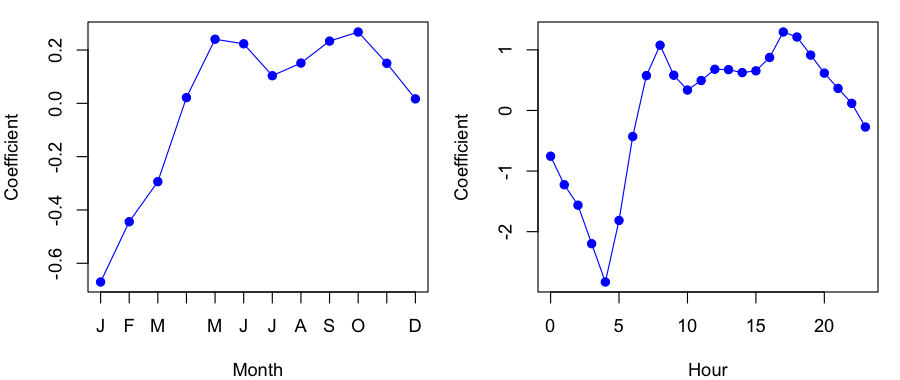
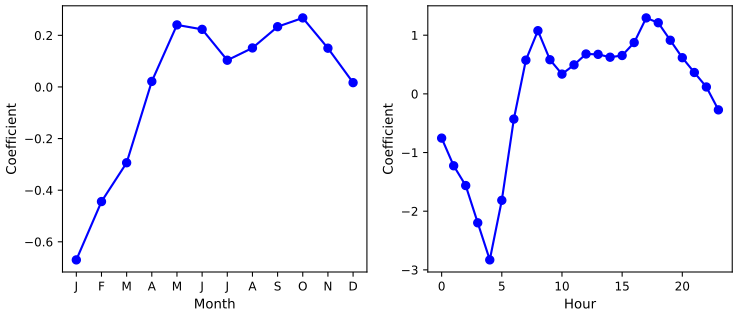
The Poisson fit gives the coefficients of Table 4.11 and the profiles of Figure 4.15, and no fitted value below 1.2. Other families are fitted in the same way: family = Gamma in R, sm.families.Gamma() in Python.
4.7.8 Where R and Python differ
Of the 59 numerical results the two scripts print with the same label, 52 agree to the printed digits; the other seven differ for the reasons below, all documented above or in the exercises.
- Naive Bayes variances (Section 4.7.5): divisor \(n_k-1\) in R, \(n_k\) in
GaussianNB; one 2005 day changes class. Rescaled, Python reproduces R. The exercise solutions below use the rescaled version, so they agree. - KNN ties (Section 4.7.6): R includes every point tied at the \(K\)th distance and breaks tied votes at random, scikit-learn keeps \(K\) points and breaks votes towards the first class. It changes \(K=3\) on Smarket and on Caravan, and several \(K\) in Exercises 13, 14 and 16; even values of \(K\) are most affected.
- Test sets: the two editions split Caravan differently (first 1,000 customers against a random 1,000); both splits are run in Python.
- Factor coding: R codes factors through
contrasts(); Python's formula interface does the same withC(x, Sum), but the levels must first be declared in the right order withpd.Categorical(otherwise months and weather levels are sorted alphabetically and the baseline changes). - Counting from 1 or 0, and class order:
lda.classes_andpredict_probacolumns follow the sorted labels in Python, the factor levels in R.
Notes on the book
Recomputing every table, figure and quoted number of the chapter, in both languages, turned up the following points. None changes a conclusion of the book.
Section 4.2: least squares and LDA do not give the same classifications
The book says that the classifications obtained by linear regression on a 0/1 response "will be the same as for" LDA. Only the direction of the linear rule is the same; the cut-points differ unless the classes are of equal size. On the Default data (balance and student), the least squares slopes are exactly 0.0282 times LDA's, yet least squares with the cut 0.5 predicts no defaulter while LDA predicts 104. On Smarket, where the classes are almost balanced, the two agree on all 252 days of 2005 (Filling the gap 4.1).
Section 4.4.1, footnote 2 (R edition): wrong equation number
The footnote contrasts the Bayes classifier with "Bayes' theorem in (4.13)"; Bayes' theorem is (4.15), and (4.13) is the softmax model. The Python edition prints (4.15).
Section 4.4.2, Figure 4.7: the threshold 0.5 does not minimise LDA's training error
The text says the threshold 0.5 "minimizes the overall error rate". That is true for the Bayes classifier, whose posterior is exact. For the fitted LDA posterior on the Default training data the overall error is 2.75% at 0.5 but 2.63% for thresholds near 0.37–0.40 (Filling the gap 4.6); the black curve of Figure 4.7 is nearly flat there, which is why the difference is invisible in the figure.
Section 4.4.4: how many predictors does the naive Bayes fit use?
The R edition says the Default data "has n = 10,000 and p = 4"; the Python edition changed this to "p = 2". Tables 4.8 and 4.9 are reproduced exactly (all eight counts) by naive Bayes with three predictors, balance, income and student (normal margins with divisor \(n_k-1\) for the first two, class proportions for student); with balance and student only, as for LDA, the counts are 9,621 / 244 / 46 / 89 instead of 9,615 / 241 / 52 / 92 (Filling the gap 4.7).
Table 4.3 and Section 4.6.2: last-digit differences
The standard error of student[Yes] in Table 4.3 is 0.236253 in both R and Python, printed by the book as 0.2362. In Section 4.6.2 the factor for cloudy weather is computed from the rounded coefficient: \(e^{-0.08}=0.923\); the fitted coefficient −0.0752 gives 0.928 (and 0.606 rather than 0.607 for rain against cloud).
Table 4.10 (R edition): a \(t\) statistic labelled \(z\)
Table 4.10 is a least squares fit, whose test statistics are \(t\) statistics; the R edition's heading says "z-statistic", the Python edition's "t-statistic". (With 8,605 residual degrees of freedom the numbers are the same.)
Section 4.6.1: which hours?
"Between 1 AM and 4 AM" (5.05 users, standard deviation 3.73) and "between 7 AM and 10 AM" (243.59 users, standard deviation 131.7) mean the hours starting at 1, 2, 3 and at 7, 8, 9; including the hours starting at 4 and 10 gives 4.54 (3.60) and 225.3 (123.5) instead.
Exercises 11 and 12 (both editions or Python edition)
Exercise 11 asks for "\(a_k\), \(b_{kj}\) and \(b_{kjl}\) in (4.33)", but (4.33) names the quadratic coefficients \(c_{kjl}\). In Exercise 12(d) the Python edition gives the friend's estimates as \(\hat\alpha_{\rm orange0}=1.2\), \(\hat\alpha_{\rm orange1}=-2\), \(\hat\alpha_{\rm orange0}=3\), \(\hat\alpha_{\rm orange1}=0.6\); the last two should be \(\hat\alpha_{\rm apple0}\) and \(\hat\alpha_{\rm apple1}\), as in the R edition. Exercise 1 calls (4.3) the "logit representation"; the logit form is (4.4), and (4.3) is its exponential (the odds).
Python lab, Caravan logistic regression: threshold 5 instead of 0.5
The 2023 lab classifies with logit_pred[:,1] > 5, a probability above 5, which never happens; this is why its table shows no predicted buyers, and the text then says that with the cut-off 0.5 "none of the test observations are predicted to purchase insurance". With the intended > 0.5 the same model flags 2 customers, neither of whom buys; the result for 0.25 (29 flagged, 9 buyers) is unaffected.
Exercises
The sixteen exercises of Section 4.8 (twelve conceptual, four applied), restated in my own words, with worked solutions (hidden). The applied solutions are run in both languages: the code is the last part of ch04_lab.R and ch04_lab.py, and the numbers quoted are their output.
Conceptual
Exercise 4.1. Show that the logistic form (4.2) and the odds form (4.3) of the logistic model are equivalent.
Solution
See Filling the gap 4.2(a): with \(\eta=\beta_0+\beta_1X\), (4.2) gives \(1-p=1/(1+e^\eta)\) and so \(p/(1-p)=e^\eta\); conversely \(p=e^\eta(1-p)\) solves to \(p=e^\eta/(1+e^\eta)\). Taking logarithms gives the logit form (4.4).
Exercise 4.2. For \(K\) normal classes \(\N(\mu_k,\sigma^2)\) with priors \(\pi_k\), show that the class maximising the posterior (4.17) is the class maximising the discriminant (4.18).
Solution
Result 4.3(a): the denominator of (4.17) and the factor \(1/(\sqrt{2\pi}\sigma)\) do not depend on \(k\); the logarithm is increasing; and after expanding \((x-\mu_k)^2\) the term \(-x^2/(2\sigma^2)\) is common to all classes. What remains is \(\delta_k(x)\).
Exercise 4.3. Now let each class have its own variance, \(X\sim\N(\mu_k,\sigma_k^2)\), \(p=1\). Show that the Bayes classifier is quadratic, not linear, in \(x\).
Solution
Taking logs of \(\pi_kf_k(x)\) and dropping \(-\frac12\log 2\pi\): \[ \delta_k(x)=-\frac{x^2}{2\sigma_k^2}+\frac{x\mu_k}{\sigma_k^2}-\frac{\mu_k^2}{2\sigma_k^2}-\log\sigma_k+\log\pi_k \]. Now the \(x^2\) term depends on \(k\) and cannot be dropped: \(\delta_k\) is a quadratic function of \(x\), and the boundary \(\delta_k=\delta_l\) solves a quadratic equation (up to two boundary points) unless \(\sigma_k=\sigma_l\). See Result 4.5.
Exercise 4.4 (the curse of dimensionality). Observations are uniform on \([0,1]^p\). To predict at a test point we use only the training points within 10% of the range of each feature around it. (a) For \(p=1\), what fraction of the data is used on average? (b) For \(p=2\)? (c) For \(p=100\)? (d) What does this say about KNN when \(p\) is large? (e) If instead we take a hypercube around the test point that contains 10% of the data on average, how long are its sides for \(p=1,2,100\)?
Solution
(a) 10%: a window of length 0.1 (shifted inwards near the edges so that it keeps its length, as in the book's example \([0.55,0.65]\)). If the window is instead cut off at 0 and 1, the average is \(0.9\times0.1+2\int_0^{0.05}(x+0.05)\,\mathrm dx=0.0975\). (b) The features are independent, so \(0.1^2=1\%\). (c) \(0.1^{100}=10^{-100}\): with any realistic \(n\), no training point at all. (d) A neighbourhood that is local in every coordinate is empty in high dimensions; to find \(K\) neighbours KNN must reach far away, so its "local" average is not local, and its bias grows. (e) A cube of side \(\ell\) holds \(\ell^p\) of the data, so \(\ell=0.1^{1/p}\): 0.1 for \(p=1\), 0.316 for \(p=2\), 0.977 for \(p=100\), i.e. almost the whole range of every feature. See Section 2.5 of the graduate course.
Exercise 4.5. LDA or QDA? (a) If the Bayes boundary is linear, which does better on the training set, and on the test set? (b) The same if the boundary is non-linear. (c) As \(n\) grows, does QDA's test accuracy relative to LDA improve, worsen or stay the same? (d) True or false: even with a linear Bayes boundary QDA will probably have a lower test error, because it can also represent a linear boundary.
Solution
(a) QDA on the training set (it is more flexible and contains LDA as a special case, so it fits the training data at least as well); LDA on the test set, because QDA's extra parameters add variance without reducing bias. (b) QDA on the training set; usually QDA on the test set, unless \(n\) is so small that its variance outweighs LDA's bias (demo preset 3 shows such a case). (c) It improves: the variance of QDA's estimates shrinks like \(1/n\), while LDA's bias (if the covariances differ) does not, and with equal covariances QDA's disadvantage vanishes as \(n\to\infty\). (d) False. QDA can represent a linear boundary, but it estimates \(Kp(p+1)/2\) covariance parameters instead of \(p(p+1)/2\), and the extra variance raises its test error for finite \(n\) (Scenario 1 of Figure 4.11: QDA 0.328 against LDA 0.313).
Exercise 4.6. A logistic regression of getting an A on hours studied \(X_1\) and undergraduate GPA \(X_2\) gives \(\hat\beta_0=-6\), \(\hat\beta_1=0.05\), \(\hat\beta_2=1\). (a) The probability of an A for a student with 40 hours and GPA 3.5? (b) How many hours would that student need for a 50% chance?
Solution
(a) \(\eta=-6+0.05\times40+3.5=-0.5\), \(\hat p=e^{-0.5}/(1+e^{-0.5})=0.3775\). (b) \(\hat p=0.5\) when \(\eta=0\): \(-6+0.05h+3.5=0\), \(h=50\) hours.
Exercise 4.7. Last year's percentage profit \(X\) is normal with variance 36 in both groups, with mean 10 for companies that paid a dividend (80% of them) and 0 for those that did not. Find the probability that a company with \(X=4\) pays a dividend.
Solution
By Bayes' theorem (4.15) with normal densities (the common factor \(1/\sqrt{72\pi}\) cancels):
\[ \Pr(\text{Yes}\given X=4)=\frac{0.8\,e^{-(4-10)^2/72}}{0.8\,e^{-(4-10)^2/72}+0.2\,e^{-(4-0)^2/72}}=\frac{0.8\times0.6065}{0.8\times0.6065+0.2\times0.8007}=0.752. \]Exercise 4.8. On a 50/50 split, logistic regression has 20% training error and 30% test error; 1-nearest neighbours has an average error of 18% over the training and test sets. Which method should be used for new data?
Solution
Logistic regression. With \(K=1\) each training point is its own nearest neighbour, so the training error of 1-NN is 0 (barring ties). An average of 18% over two equal halves then means a test error of 36%, worse than logistic regression's 30%. Only test error measures performance on new data.
Exercise 4.9. (a) What fraction of people with odds 0.37 of defaulting will default? (b) What are the odds of someone with a 16% chance of default?
Solution
(a) \(p=\text{odds}/(1+\text{odds})=0.37/1.37=0.27\). (b) \(0.16/0.84=0.19\).
Exercise 4.10. For \(p=1\), redo the calculation (4.32) and give \(a_k\) and \(b_{k1}\) in terms of \(\pi_k,\pi_K,\mu_k,\mu_K,\sigma^2\).
Solution
\[ \log\frac{\pi_kf_k(x)}{\pi_Kf_K(x)}=\log\frac{\pi_k}{\pi_K}-\frac{(x-\mu_k)^2-(x-\mu_K)^2}{2\sigma^2}=\log\frac{\pi_k}{\pi_K}-\frac{\mu_k^2-\mu_K^2}{2\sigma^2}+\frac{\mu_k-\mu_K}{\sigma^2}x \]. So \(a_k=\log(\pi_k/\pi_K)-(\mu_k^2-\mu_K^2)/(2\sigma^2)\) and \(b_{k1}=(\mu_k-\mu_K)/\sigma^2\) (Filling the gap 4.8(c)).
Exercise 4.11. Give \(a_k\), \(b_{kj}\) and the quadratic coefficients \(c_{kjl}\) of (4.33) in terms of \(\pi_k,\pi_K,\mu_k,\mu_K,\Sigma_k,\Sigma_K\).
Solution
\[ a_k=\log\frac{\pi_k}{\pi_K}-\frac12\log\frac{|\Sigma_k|}{|\Sigma_K|}-\frac12(\mu_k^\T\Sigma_k^{-1}\mu_k-\mu_K^\T\Sigma_K^{-1}\mu_K) \], \(b_{kj}=[\Sigma_k^{-1}\mu_k-\Sigma_K^{-1}\mu_K]_j\), \(c_{kjl}=-\frac12[\Sigma_k^{-1}-\Sigma_K^{-1}]_{jl}\). Derivation in Filling the gap 4.8(b); setting \(\Sigma_k=\Sigma_K=\Sigma\) recovers (4.32), with \(c_{kjl}=0\).
Exercise 4.12. You fit \[ \widehat{\Pr}(\text{orange}\given x)=\sigma(\hat\beta_0+\hat\beta_1x) \]; a friend fits the softmax model (4.13) with coefficients \[ \hat\alpha_{\rm orange0},\hat\alpha_{\rm orange1},\hat\alpha_{\rm apple0},\hat\alpha_{\rm apple1} \]. (a) Your log-odds of orange against apple? (b) Your friend's? (c) If \(\hat\beta_0=2\), \(\hat\beta_1=-1\), what are your friend's estimates? (d) If your friend gets \(1.2,-2,3,0.6\) (orange intercept and slope, apple intercept and slope), what are yours? (e) On 2,000 test points, how often do the two models' predicted labels agree?
Solution
(a) \(\hat\beta_0+\hat\beta_1x\). (b) \[ (\hat\alpha_{\rm orange0}-\hat\alpha_{\rm apple0})+(\hat\alpha_{\rm orange1}-\hat\alpha_{\rm apple1})x \], by (4.14). (c) Only the differences are determined (Result 4.2): \(\hat\alpha_{\rm orange0}-\hat\alpha_{\rm apple0}=2\), \(\hat\alpha_{\rm orange1}-\hat\alpha_{\rm apple1}=-1\); for instance \((2,-1)\) and \((0,0)\), or any common shift of both. (d) \(\hat\beta_0=1.2-3=-1.8\), \(\hat\beta_1=-2-0.6=-2.6\). (e) Always (100%): the two fits are the same model in two parametrisations, so they give the same probabilities and labels for every \(x\). (If the friend fitted separately on the same data, maximum likelihood would also give the same fitted probabilities, because the likelihood depends on the differences only.)
Applied
Exercise 4.13 (Weekly). 1,089 weekly returns of the S&P 500, 1990–2010, with the same variables as Smarket. (a) Summarise the data. (b) Logistic regression of Direction on the five lags and Volume, all weeks: which predictors are significant? (c) Its confusion matrix and accuracy: what kinds of mistake does it make? (d) Train 1990–2008 with Lag2 only and test on 2009–2010: confusion matrix and accuracy. (e)–(h) The same with LDA, QDA, KNN with \(K=1\) and naive Bayes. (i) Which is best? (j) Try other predictors, transformations and values of \(K\).
Solution
R
fit13 <- glm(Direction ~ Lag1 + Lag2 + Lag3 + Lag4 + Lag5 + Volume, data = Weekly, family = binomial)
show("Ex13b p-values (Lag1..Lag5, Volume)", summary(fit13)$coef[-1, 4])
pred13 <- ifelse(fitted(fit13) > 0.5, "Up", "Down")
show_table("Ex13c confusion (all weeks)", table(pred13, Weekly$Direction))
show("Ex13c accuracy", acc(pred13, Weekly$Direction))
tr13 <- Weekly$Year <= 2008
te13 <- Weekly[!tr13, ]
fit13d <- glm(Direction ~ Lag2, data = Weekly, family = binomial, subset = tr13)
pred13d <- ifelse(predict(fit13d, te13, type = "response") > 0.5, "Up", "Down")
show_table("Ex13d confusion, logistic on Lag2 (2009-2010)", table(pred13d, te13$Direction))
show("Ex13d-h accuracy: logistic, LDA, QDA, KNN-1, naive Bayes", c(
  acc(pred13d, te13$Direction),
  acc(predict(lda(Direction ~ Lag2, data = Weekly, subset = tr13), te13)$class, te13$Direction),
  acc(predict(qda(Direction ~ Lag2, data = Weekly, subset = tr13), te13)$class, te13$Direction),
  { set.seed(1); acc(knn(cbind(Weekly$Lag2[tr13]), cbind(te13$Lag2), Weekly$Direction[tr13], k = 1), te13$Direction) },
  acc(predict(naiveBayes(Direction ~ Lag2, data = Weekly, subset = tr13), te13), te13$Direction)))
set.seed(1)
show("Ex13j KNN on Lag2, K = 1..15", sapply(1:15, function(k)
  acc(knn(cbind(Weekly$Lag2[tr13]), cbind(te13$Lag2), Weekly$Direction[tr13], k = k), te13$Direction)), 3)
show("Ex13j LDA on Lag1 + Lag2, logistic on Lag2 + Lag2^2", c(
  acc(predict(lda(Direction ~ Lag1 + Lag2, data = Weekly, subset = tr13), te13)$class, te13$Direction),
  acc(ifelse(predict(glm(Direction ~ Lag2 + I(Lag2^2), data = Weekly, family = binomial, subset = tr13),
                     te13, type = "response") > 0.5, "Up", "Down"), te13$Direction)))
Python
yw = (Weekly.Direction == "Up").astype(int)
lag6 = ["Lag1", "Lag2", "Lag3", "Lag4", "Lag5", "Volume"]
fit13 = logit_fit(Weekly[lag6], yw)
show("Ex13b p-values (Lag1..Lag5, Volume)", fit13.pvalues.values[1:])
pred13 = np.where(fit13.fittedvalues > 0.5, "Up", "Down")
show_table("Ex13c confusion (all weeks)", pred13, Weekly.Direction)
show("Ex13c accuracy", np.mean(pred13 == Weekly.Direction))
tr13 = (Weekly.Year <= 2008).values
Xtr, Xte = Weekly.loc[tr13, ["Lag2"]], Weekly.loc[~tr13, ["Lag2"]]
Ltr, Lte = Weekly.Direction[tr13].values, Weekly.Direction[~tr13].values
fit13d = logit_fit(Xtr, yw[tr13])
pred13d = np.where(fit13d.predict(sm.add_constant(Xte, has_constant="add")) > 0.5, "Up", "Down")
show_table("Ex13d confusion, logistic on Lag2 (2009-2010)", pred13d, Lte)
show("Ex13d-h accuracy: logistic, LDA, QDA, KNN-1, naive Bayes", [
    np.mean(pred13d == Lte),
    np.mean(LDA().fit(Xtr, Ltr).predict(Xte) == Lte),
    np.mean(QDA().fit(Xtr, Ltr).predict(Xte) == Lte),
    np.mean(KNeighborsClassifier(1).fit(Xtr, Ltr).predict(Xte) == Lte),
    np.mean(nb_divisor_n1(Xtr, Ltr).predict(Xte) == Lte)])
show("Ex13j KNN on Lag2, K = 1..15",
     [np.mean(KNeighborsClassifier(k).fit(Xtr, Ltr).predict(Xte) == Lte) for k in range(1, 16)], 3)
Xq = Weekly[["Lag2"]].assign(Lag2sq=Weekly.Lag2 ** 2)
pq = logit_fit(Xq[tr13], yw[tr13]).predict(sm.add_constant(Xq[~tr13], has_constant="add"))
show("Ex13j LDA on Lag1 + Lag2, logistic on Lag2 + Lag2^2", [
    np.mean(LDA().fit(Weekly.loc[tr13, ["Lag1", "Lag2"]], Ltr).predict(Weekly.loc[~tr13, ["Lag1", "Lag2"]]) == Lte),
    np.mean(np.where(pq > 0.5, "Up", "Down") == Lte)])
Ex13b p-values (Lag1..Lag5, Volume): 0.1181 0.0296 0.5469 0.2937 0.5833 0.5377 Ex13c confusion (all weeks): 54 48 / 430 557 Ex13c accuracy: 0.5611 Ex13d confusion, logistic on Lag2 (2009-2010): 9 5 / 34 56 Ex13d-h accuracy: logistic, LDA, QDA, KNN-1, naive Bayes: 0.6250 0.6250 0.5865 0.5000 0.5865 Ex13j KNN on Lag2, K = 1..15 (R): 0.500 0.519 0.548 0.596 0.519 0.538 0.538 0.538 0.548 0.577 0.567 0.606 0.596 0.558 0.587 Ex13j KNN on Lag2, K = 1..15 (Python): 0.500 0.452 0.558 0.577 0.529 0.510 0.548 0.548 0.548 0.567 0.558 0.567 0.587 0.567 0.587 Ex13j LDA on Lag1 + Lag2, logistic on Lag2 + Lag2^2: 0.5769 0.6250(a) Volume grows strongly with Year (as for Smarket); the lags are nearly uncorrelated with each other and with Today; 605 of the 1,089 weeks are Up. (b) Only Lag2 is significant at 5% (p = 0.030). (c) The model predicts Up in 987 of 1,089 weeks: it catches 557 of the 605 Up weeks (92%) but only 54 of the 484 Down weeks (11%); its 56.1% training accuracy is little better than always saying Up (55.6%). (d)–(h) On the 104 held-out weeks, logistic regression and LDA on Lag2 are right 62.5% of the time, QDA and naive Bayes 58.7% (both predict Up every week, which is right 61 times out of 104), KNN with \(K=1\) 50%. (i) Logistic regression and LDA. (j) No variant tried beats 62.5%: Lag1 + Lag2 in LDA gives 57.7%, adding Lag2\(^2\) to logistic regression changes nothing, and the best KNN (K = 12 in R, 60.6%) is chosen on the test set itself, which flatters it. The KNN accuracies differ between R and Python for several \(K\) because of ties (Section 4.7.8); everything else agrees.
Exercise 4.14 (Auto). (a) Create
mpg01= 1 if a car's mpg is above the median. (b) Which other variables are associated with it? (c) Split into training and test sets. (d)–(g) Test errors of LDA, QDA, logistic regression and naive Bayes on the most associated variables. (h) KNN with several \(K\).Solution
R
Auto14 <- Auto
Auto14$mpg01 <- factor(as.integer(Auto14$mpg > median(Auto14$mpg)))
show("Ex14a median mpg, share of 1s", c(median(Auto$mpg), mean(Auto14$mpg01 == "1")))
show("Ex14b cor(mpg01, cylinders, displacement, horsepower, weight, acceleration, year)",
     cor(as.integer(Auto14$mpg01 == "1"), Auto14[, c("cylinders", "displacement", "horsepower", "weight",
                                                     "acceleration", "year")]), 3)
tr14 <- seq_len(nrow(Auto14)) %% 2 == 1        # odd rows train, even rows test
te14 <- Auto14[!tr14, ]
f14 <- mpg01 ~ cylinders + displacement + horsepower + weight
p14 <- predict(glm(f14, data = Auto14, family = binomial, subset = tr14), te14, type = "response")
show("Ex14d-g test error: LDA, QDA, logistic, naive Bayes", c(
  1 - acc(predict(lda(f14, data = Auto14, subset = tr14), te14)$class, te14$mpg01),
  1 - acc(predict(qda(f14, data = Auto14, subset = tr14), te14)$class, te14$mpg01),
  1 - acc(as.integer(p14 > 0.5), te14$mpg01),
  1 - acc(predict(naiveBayes(f14, data = Auto14, subset = tr14), te14), te14$mpg01)))
v14 <- c("cylinders", "displacement", "horsepower", "weight")
m14 <- colMeans(Auto14[tr14, v14]); s14 <- apply(Auto14[tr14, v14], 2, sd)
Z14 <- scale(Auto14[, v14], center = m14, scale = s14)
set.seed(1)
show("Ex14h KNN test error, K = 1..10 (standardised)", sapply(1:10, function(k)
  1 - acc(knn(Z14[tr14, ], Z14[!tr14, ], Auto14$mpg01[tr14], k = k), te14$mpg01)), 3)
Python
Auto = common.isl_data("Auto", na_values="?").dropna().reset_index(drop=True)    # 392 cars, as in R
Auto["mpg01"] = (Auto.mpg > Auto.mpg.median()).astype(int)
show("Ex14a median mpg, share of 1s", [Auto.mpg.median(), Auto.mpg01.mean()])
v6 = ["cylinders", "displacement", "horsepower", "weight", "acceleration", "year"]
show("Ex14b cor(mpg01, cylinders, displacement, horsepower, weight, acceleration, year)",
     [np.corrcoef(Auto.mpg01, Auto[v])[0, 1] for v in v6], 3)
tr14 = (np.arange(len(Auto)) % 2 == 0)        # rows 1, 3, 5, ... (R's odd rows) train
v14 = ["cylinders", "displacement", "horsepower", "weight"]
Xtr, Xte, ytr, yte = Auto.loc[tr14, v14], Auto.loc[~tr14, v14], Auto.mpg01[tr14].values, Auto.mpg01[~tr14].values
p14 = logit_fit(Xtr, ytr).predict(sm.add_constant(Xte))
show("Ex14d-g test error: LDA, QDA, logistic, naive Bayes", [
    np.mean(LDA().fit(Xtr, ytr).predict(Xte) != yte), np.mean(QDA().fit(Xtr, ytr).predict(Xte) != yte),
    np.mean((p14.values > 0.5) != yte), np.mean(nb_divisor_n1(Xtr, ytr).predict(Xte) != yte)])
Ztr, Zte = (Xtr - Xtr.mean()) / Xtr.std(), (Xte - Xtr.mean()) / Xtr.std()
show("Ex14h KNN test error, K = 1..10 (standardised)",
     [np.mean(KNeighborsClassifier(k).fit(Ztr, ytr).predict(Zte) != yte) for k in range(1, 11)], 3)
Ex14a median mpg, share of 1s: 22.7500 0.5000 Ex14b cor(mpg01, cylinders, displacement, horsepower, weight, acceleration, year): -0.759 -0.753 -0.667 -0.758 0.347 0.430 Ex14d-g test error: LDA, QDA, logistic, naive Bayes: 0.0918 0.1122 0.1224 0.1122 Ex14h KNN test error, K = 1..10 (R): 0.122 0.128 0.102 0.102 0.097 0.102 0.102 0.107 0.107 0.102 Ex14h KNN test error, K = 1..10 (Python): 0.122 0.138 0.102 0.097 0.097 0.107 0.102 0.107 0.107 0.107(a) The median of the 392 cars (the Python script drops the five with missing horsepower, as the R package does) is 22.75 mpg, so exactly half are 1. (b) Boxplots and correlations point to cylinders, displacement, horsepower and weight (correlations −0.67 to −0.76); year and acceleration are weaker. (c) A reproducible split usable in both languages: odd-numbered rows train, even-numbered rows test (196 each). (d)–(g) Test errors 9.2% (LDA), 11.2% (QDA), 12.2% (logistic regression), 11.2% (naive Bayes). (h) On standardised inputs KNN reaches 9.7% at \(K=5\) in both languages; \(K=1\) gives 12.2%. With 196 test cars one error is 0.5%, so the methods are hard to separate.
Exercise 4.15 (writing functions). (a) A function
Power()that prints \(2^3\). (b)Power2(x, a)that prints \(x^a\). (c) Use it for \(10^3\), \(8^{17}\), \(131^3\). (d)Power3(x, a)that returns \(x^a\). (e) Plot \(f(x)=x^2\) for \(x=1,\dots,10\), with labelled axes and a title, optionally on log scales. (f)PlotPower(x, a)that plots \(x^a\) against \(x\).Solution
R
Power <- function() print(2^3)
Power2 <- function(x, a) print(x^a)
Power2(10, 3); Power2(8, 17); Power2(131, 3)
Power3 <- function(x, a) {
  result <- x^a
  return(result)
}
x <- 1:10
plot(x, Power3(x, 2), log = "xy", xlab = "x",
     ylab = "x^2", main = "f(x) = x^2 (log scales)")
PlotPower <- function(x, a)
  plot(x, Power3(x, a), xlab = "x", ylab = paste0("x^", a))
PlotPower(1:10, 3)
Python
import numpy as np
import matplotlib.pyplot as plt
def Power(): print(2 ** 3)
def Power2(x, a): print(x ** a)
Power2(10, 3); Power2(8, 17); Power2(131, 3)
def Power3(x, a):
    result = x ** a
    return result
x = np.arange(1, 11)
fig, ax = plt.subplots()
ax.plot(x, Power3(x, 2), "o-"); ax.set_xscale("log"); ax.set_yscale("log")
ax.set_xlabel("x"); ax.set_ylabel("x^2"); ax.set_title("f(x) = x^2 (log scales)")
def PlotPower(x, a):
    fig, ax = plt.subplots(); ax.plot(x, Power3(x, a), "o-")
    ax.set_xlabel("x"); ax.set_ylabel("x^%d" % a)
PlotPower(np.arange(1, 11), 3)
The printed values are 8, then 1000, 2251799813685248 and 2248091. In R, \(8^{17}\) is stored as a double and prints as
2.2518e+15unless more digits are requested; Python integers are exact. On log–log axes \(x^2\) is a straight line of slope 2.Exercise 4.16 (Boston). Predict whether a suburb's crime rate is above the median, with logistic regression, LDA, naive Bayes and KNN on several subsets of the predictors. Describe the findings.
Solution
R
Boston16 <- ISLR2::Boston          # MASS (loaded above) has an older Boston with 14 columns
Boston16$crim01 <- factor(as.integer(Boston16$crim > median(Boston16$crim)))
tr16 <- seq_len(nrow(Boston16)) %% 2 == 1
te16 <- Boston16[!tr16, ]
for (vars in list(c("nox", "rad", "dis", "age", "tax", "indus"),
                  setdiff(names(ISLR2::Boston), "crim"))) {
  f16 <- reformulate(vars, "crim01")
  p16 <- predict(glm(f16, data = Boston16, family = binomial, subset = tr16), te16, type = "response")
  Z16 <- scale(Boston16[, vars], center = colMeans(Boston16[tr16, vars]), scale = apply(Boston16[tr16, vars], 2, sd))
  set.seed(1)
  show(sprintf("Ex16 test error with %d predictors: logistic, LDA, naive Bayes, KNN-1, KNN-5, KNN-10", length(vars)), c(
    1 - acc(as.integer(p16 > 0.5), te16$crim01),
    1 - acc(predict(lda(f16, data = Boston16, subset = tr16), te16)$class, te16$crim01),
    1 - acc(predict(naiveBayes(f16, data = Boston16, subset = tr16), te16), te16$crim01),
    sapply(c(1, 5, 10), function(k) 1 - acc(knn(Z16[tr16, ], Z16[!tr16, ], Boston16$crim01[tr16], k = k), te16$crim01))))
}
Python
Boston = common.isl_data("Boston", index_col=0)
Boston["crim01"] = (Boston.crim > Boston.crim.median()).astype(int)
tr16 = (np.arange(len(Boston)) % 2 == 0)
for vars16 in (["nox", "rad", "dis", "age", "tax", "indus"], [c for c in Boston.columns if c not in ("crim", "crim01")]):
    Xtr, Xte = Boston.loc[tr16, vars16], Boston.loc[~tr16, vars16]
    ytr, yte = Boston.crim01[tr16].values, Boston.crim01[~tr16].values
    p16 = logit_fit(Xtr, ytr).predict(sm.add_constant(Xte))
    Ztr, Zte = (Xtr - Xtr.mean()) / Xtr.std(), (Xte - Xtr.mean()) / Xtr.std()
    show("Ex16 test error with %d predictors: logistic, LDA, naive Bayes, KNN-1, KNN-5, KNN-10" % len(vars16), [
        np.mean((p16.values > 0.5) != yte), np.mean(LDA().fit(Xtr, ytr).predict(Xte) != yte),
        np.mean(nb_divisor_n1(Xtr, ytr).predict(Xte) != yte)]
        + [np.mean(KNeighborsClassifier(k).fit(Ztr, ytr).predict(Zte) != yte) for k in (1, 5, 10)])
Ex16 test error with 6 predictors: logistic, LDA, naive Bayes, KNN-1, KNN-5, KNN-10: R: 0.1383 0.1423 0.1700 0.0711 0.0751 0.0949 Python: ... 0.0909 for KNN-10, the rest equal Ex16 test error with 12 predictors: logistic, LDA, naive Bayes, KNN-1, KNN-5, KNN-10: 0.0870 0.1265 0.1858 0.0949 0.0988 0.1107 (both)Odd rows train and even rows test (253 suburbs each). Six predictors chosen for their strong association with crime (nitrogen oxides, access to radial highways, distance to employment centres, age, tax rate, industry) give 13.8% (logistic), 14.2% (LDA) and 17.0% (naive Bayes) errors, but KNN does much better, 7.1% with \(K=1\): high-crime suburbs are geographically clustered, and nearest neighbours in these variables are essentially neighbouring suburbs. With all twelve predictors logistic regression improves to 8.7% while KNN worsens (9.5% for \(K=1\)), since irrelevant dimensions dilute the distances. Naive Bayes is worst throughout, as these predictors are strongly correlated (Result 4.6). (Note that R's
library(MASS)masksISLR2::Bostonwith an older 14-column version; the R code namesISLR2::Bostonexplicitly.)
Demonstrations for this chapter
Each demonstration runs in the browser on the book's own data (or on data simulated in the page) and links back to these notes. The ▶ Demo boxes above open them already set to the case under discussion.
| Demonstration | What you can see | Sections and results |
|---|---|---|
| Thresholds and the ROC curve on the Default data | LDA, two logistic regressions and naive Bayes fitted in the browser; a threshold slider with the confusion matrix, sensitivity, specificity and predictive values, the error rates of Figure 4.7 and the ROC curve with its AUC. Presets: 1 Table 4.4; 2 Table 4.5; 3 Figure 4.8; 4 Table 4.8; 5 the cost-weighted threshold 1/11. | 4.3, 4.4.2, 4.4.4; Definition 4.2, Result 4.4, Filling the gap 4.6 |
| LDA, QDA, logistic regression and naive Bayes on simulated classes | Two normal classes with adjustable correlations, separation and sample size; the Bayes, LDA, QDA, logistic and naive Bayes boundaries and their training and test errors. Presets: 1 Figure 4.9, left; 2 Figure 4.9, right; 3 10 points per class; 4 500 per class; 5 Scenario 2. | 4.4.3, 4.5.1, 4.5.2; Result 4.5, Result 4.6 |
| Poisson regression on the Bikeshare data | Least squares and Poisson regression with a choice of predictors: month and hour effects, the mean–variance plot of the hour-by-month cells, fitted values against each other, the weather effects as factors, negative fits and overdispersion. Presets: 1 Tables 4.10–4.11; 2 weather factors; 3 overdispersion; 4 negative fits; 5 hour only. | 4.6.1, 4.6.2, 4.6.3; Result 4.7 |
The code: code/ch04_classification.py makes every figure and table of the chapter and the demonstrations' data; code/ch04_lab.R and code/ch04_lab.py are the lab and the applied exercises (see the code index).
References
- James, G., Witten, D., Hastie, T. and Tibshirani, R. (2021). An Introduction to Statistical Learning with Applications in R, 2nd edition. Springer, New York. Chapter 4, pp. 129–195. www.statlearning.com.
- James, G., Witten, D., Hastie, T., Tibshirani, R. and Taylor, J. (2023). An Introduction to Statistical Learning with Applications in Python. Springer, Cham. Chapter 4, pp. 135–199.
- Hastie, T., Tibshirani, R. and Friedman, J. (2009). The Elements of Statistical Learning: Data Mining, Inference, and Prediction, 2nd edition. Springer, New York.
- Agresti, A. (2013). Categorical Data Analysis, 3rd edition. Wiley, Hoboken, NJ.
- Efron, B. (1975). The efficiency of logistic regression compared to normal discriminant analysis. Journal of the American Statistical Association, 70(352), 892–898.
- Fisher, R. A. (1936). The use of multiple measurements in taxonomic problems. Annals of Eugenics, 7(2), 179–188.
- Hanley, J. A. and McNeil, B. J. (1982). The meaning and use of the area under a receiver operating characteristic (ROC) curve. Radiology, 143(1), 29–36.
- McCullagh, P. and Nelder, J. A. (1989). Generalized Linear Models, 2nd edition. Chapman and Hall, London.
- Nelder, J. A. and Wedderburn, R. W. M. (1972). Generalized linear models. Journal of the Royal Statistical Society, Series A, 135(3), 370–384.
- Ng, A. Y. and Jordan, M. I. (2002). On discriminative vs. generative classifiers: a comparison of logistic regression and naive Bayes. Advances in Neural Information Processing Systems, 14, 841–848.
- Simpson, E. H. (1951). The interpretation of interaction in contingency tables. Journal of the Royal Statistical Society, Series B, 13(2), 238–241.
The numerical statements in the text (Tables 4.1–4.5 and 4.8–4.11 and the numbers quoted with them, the Newton fits against statsmodels and R, the score equations, the baseline invariance of the multinomial model, the discriminant and log-odds formulas, the AUC identity, the six scenarios, the Poisson factors and the dispersion, the agreement of the R and Python labs, the book points listed above and the answers to the exercises) were confirmed numerically.