Exemplar-based Methods
Exemplar-based (instance-based, memory-based) methods keep the training data and make a prediction at a new input by looking at the stored examples that are most similar to it. The chapter has three parts: the K nearest neighbour classifier, whose predictive distribution is just the label frequencies in a neighbourhood and which, remarkably, is within a factor of two of the best possible classifier as the sample grows, but suffers badly from the curse of dimensionality; the learning of the distance itself, from convex Mahalanobis methods (LMNN, NCA, latent coincidence analysis) to the ranking losses of deep metric learning (contrastive, triplet, N-pairs) and the tricks that make them affordable; and kernel density estimation, which puts a small bump on every data point and leads to the Nadaraya-Watson and local linear regression estimators. The notes prove every statement the book leaves as "it can be shown", test the claims on simulated problems, the wine and digits data, and show where the book's formulas need a correction.
Ch. 1 Introduction Ch. 2 Univariate probability Ch. 3 Multivariate probability Ch. 4 Statistics Ch. 5 Decision theory Ch. 6 Information theory Ch. 7 Linear algebra Ch. 8 Optimisation Ch. 9 Discriminant analysis Ch. 10 Logistic regression Ch. 11 Linear regression Ch. 12 GLMs Ch. 13 Networks for tabular data Ch. 14 Networks for images Ch. 15 Networks for sequences Ch. 16 Exemplar-based methods Ch. 17 Kernel methods Ch. 18 Trees and boosting Ch. 19 Fewer labels Ch. 20 Dimensionality reduction Ch. 21 Clustering Ch. 22 Recommender systems Ch. 23 Graph embeddings
How to read these notes
They follow the book. Sections carry the book's numbers (16.1.2, 16.2.4.3, ...) and equations the book numbers keep their numbers, e.g. \((16.33)\); equations without a number are steps the book skips. Chapter 16 is not starred in the book, and it has no end-of-chapter exercises: the six exercises at the end are my own.
Filling the gaps. Wherever the book writes "it can be shown", quotes a result from the literature, or states a formula without derivation, an orange Filling the gap box gives the full argument. Proofs start hidden: open one with its bar, or use the buttons below.
Figures and demonstrations. Every computed figure is reproduced by the Python code; Figures 16.3a, 16.4, 16.5, 16.6b and 16.7 are hand-drawn sketches and are not reproduced. Figures 16.1, 16.2 and 16.10 use small simulated data sets because the book's own point sets are not available offline, and Figure 16.6a is a redrawing with computed points; the captions say so. Further figures labelled 16.S1 to 16.S9 are my own and illustrate the gaps. The ▶ Demo boxes open an interactive demonstration set to the case being discussed.
Main reference
K. P. Murphy, Probabilistic Machine Learning: An Introduction, MIT Press (2022), Chapter 16, pages 547–565 (book page: probml.github.io/pml-book/book1.html). Section, equation, figure and exercise numbers below refer to this book. The explanations, derivations, figures and code are my own.
Companion courses
Nearest neighbours, kernel smoothing and density estimation are also developed, in other notation, elsewhere on this site. Where a result is proved in full there, these notes give the statement and a short sketch and link to it.
- Bayesian and Probabilistic Machine Learning (Bishop): 2.5.1 kernel density estimators, 2.5.2 nearest-neighbour methods, 2.5.3 consistency and the Cover–Hart bound, 6.3.1 the Nadaraya–Watson model.
- Elements of Statistical Learning (Hastie, Tibshirani, Friedman): 13.3 k-nearest-neighbor classifiers, 13.4 adaptive nearest-neighbor methods (a learned metric), 13.5 computational considerations, 6.1 one-dimensional kernel smoothers, 6.1.1 local linear regression, 6.6.1 kernel density estimation.
- Nonparametric Statistical Inference (Wasserman): 6.3 kernel density estimation (the bias-variance expansion and the bandwidth), 5.2 linear smoothers and 5.4 local regression.
- All of Statistics: 20.3 kernel density estimation and 20.4 nonparametric regression.
What this chapter adds: the 1-NN risk and the Cover–Hart bound for many classes with a full proof, the cost of exact search and locality-sensitive hashing, open-set recognition, the convex (LMNN), probabilistic (NCA) and latent-variable (LCA) ways of learning a Mahalanobis metric with the gradients and the EM updates worked out, the modern ranking losses (contrastive, triplet, N-pairs/InfoNCE) with hard-negative mining and the proxy upper bound, and the derivation of the KNN classifier from kernel density estimation.
The chapter at a glance
- 16.1 The KNN predictive distribution (16.1) and the Voronoi cells of 1-NN; the 1-NN rule is within a factor of two of the Bayes error (gap 16.1); the curse of dimensionality (gap 16.2); exact and approximate search (gap 16.3); open-set recognition as thresholding the nearest-exemplar distance (gap 16.4).
- 16.2.1 Learning a Mahalanobis matrix: LMNN is a convex problem (gap 16.5), NCA maximises the expected number of correct leave-one-out votes (gap 16.6), latent coincidence analysis has a closed-form marginal likelihood and an exact EM algorithm (gap 16.7).
- 16.2.2–16.2.6 Deep metric learning: normalised embeddings, the N-pairs/InfoNCE loss and its temperature limit (gap 16.8), the triplet loss and hard negatives (gap 16.9), the proxy bound that makes triplet training linear in \(N\) (gap 16.10), sampling the sphere (gap 16.11).
- 16.3 Density kernels and the Parzen estimator (gap 16.12), the bandwidth rule (gap 16.13), KNN as a generative classifier (gap 16.14), the Nadaraya–Watson mean and variance (gap 16.15) and locally weighted regression (gap 16.16).
Notation. Data \(\mathcal D=\{(\bm x_n,y_n)\}_{n=1}^N\); \(\mathcal N_K(\bm x,\mathcal D)\) is the set of the \(K\) training inputs closest to \(\bm x\); \(\ind(\cdot)\) is the indicator; \([z]_+=\max(z,0)\); \(\hat{\bm e}=\bm e/\|\bm e\|_2\) is a normalised embedding; \(K_h(u)=K(u/h)/h\) is a scaled density kernel. \(R^*\) is the Bayes error and \(\eta_c(\bm x)=p(y=c\given\bm x)\).
Prerequisites. Chapters 2 to 5 of the book (probability, the multivariate Gaussian, decision theory), the Mahalanobis distance of Chapter 3, and the softmax and logistic loss of Chapter 10.
16.1 K nearest neighbor (KNN) classification
pp. 547–548 So far the models of the book were parametric: a fixed-length vector \(\bm\theta\) is estimated from the data and the data are then discarded. Chapter 16 keeps the data. An exemplar-based model defines its prediction at a test input \(\bm x\) through a similarity \(s(\bm x,\bm x_n)\) or a distance \(d(\bm x,\bm x_n)\) to each stored training input, so the effective number of parameters grows with \(N\). The simplest instance is the K nearest neighbour classifier: find the \(K\) training inputs closest to \(\bm x\), \(\mathcal N_K(\bm x,\mathcal D)\), and report the label frequencies among them, \[ p(y=c\given\bm x,\mathcal D)=\frac1K\sum_{n\in\mathcal N_K(\bm x,\mathcal D)}\ind(y_n=c). \tag{16.1} \] Returning the whole distribution is useful, and the majority label (the mode) is the usual hard prediction. The two ingredients are the size \(K\) of the neighbourhood and the distance. The standard choice is the Mahalanobis distance \[ d_{\bm M}(\bm x,\bm x')=\sqrt{(\bm x-\bm x')^\T\bm M(\bm x-\bm x')}, \tag{16.2, 16.3} \] with \(\bm M\) positive definite (\(\bm M=\bm I\) is Euclidean). Since \(\bm M=\bm W^\T\bm W\) for some matrix \(\bm W\), \(d_{\bm M}(\bm x,\bm x')=\|\bm W\bm x-\bm W\bm x'\|_2\): the Mahalanobis distance is the Euclidean distance after a linear map. Section 16.2 learns \(\bm M\) from data.
The classifier is simple and yet statistically strong. As \(N\to\infty\) the error of the 1-NN rule is at most about twice the Bayes error, the error of the best possible classifier; the precise statement and its proof (the book only cites [CH67; CD14]) is the first gap box. The word "asymptotically" matters, because the convergence rate can be terrible in high dimension (Section 16.1.2).
Filling the gap 16.1: the Cover–Hart bound, \(R^*\le R_{\rm 1NN}\le R^*\big(2-\tfrac{C}{C-1}R^*\big)\) p. 547, [CH67; CD14]
Statement and proof
Setting. \((\bm X,Y)\) has \(Y\in\{1,\dots,C\}\), \(\eta_c(\bm x)=p(y=c\given\bm x)\) and the Bayes rule \(\arg\max_c\eta_c\) has error \(R^*=\E[r(\bm X)]\) with \(r(\bm x)=1-\max_c\eta_c(\bm x)\). The training pairs \((\bm X_n,Y_n)\) are i.i.d. and independent of \((\bm X,Y)\). Let \(\bm X_{(1)}\) be the training input nearest to \(\bm X\) and \(Y_{(1)}\) its label; the asymptotic 1-NN risk is \(R_{\rm 1NN}=\lim_{N\to\infty}\Pr(Y_{(1)}\ne Y)\). Assume every \(\eta_c\) is continuous (Cover and Hart assume continuity almost everywhere; the argument below goes through at every continuity point).
Claim. \(R_{\rm 1NN}=\E\big[1-\sum_c\eta_c(\bm X)^2\big]\), and \(R^*\le R_{\rm 1NN}\le 2R^*-\frac{C}{C-1}R^{*2}\le2R^*\). For \(C=2\) the upper bound is \(2R^*(1-R^*)\).
Step 1: the nearest neighbour converges to the query. Let \(\bm x\) be in the support of \(P_{\bm X}\). For \(\varepsilon>0\), \(q_\varepsilon=\Pr(\|\bm X-\bm x\|<\varepsilon)>0\) by the definition of the support, so \(\Pr(\|\bm X_{(1)}-\bm x\|\ge\varepsilon)=(1-q_\varepsilon)^N\to0\). The set of \(\bm x\) outside the support has probability 0 (in \(\R^D\), a countable cover by balls of probability zero), so \(\bm X_{(1)}\to\bm X\) in probability.
Step 2: the risk. Condition on \(\bm X=\bm x\) and on the training inputs. The labels \(Y\) and \(Y_{(1)}\) are then independent with distributions \(\bm\eta(\bm x)\) and \(\bm\eta(\bm X_{(1)})\), so \[ \Pr(Y_{(1)}\ne Y\given\bm X=\bm x,\bm X_{(1)})=1-\sum_c\eta_c(\bm X_{(1)})\,\eta_c(\bm x)\;\longrightarrow\;1-\sum_c\eta_c(\bm x)^2 \] in probability by Step 1 and continuity. The left side lies in \([0,1]\), so bounded convergence gives \(R_{\rm 1NN}=\E[1-\sum_c\eta_c(\bm X)^2]\).
Step 3: pointwise bounds. Fix \(\bm x\), let \(c^*\) be the Bayes class and \(r=1-\eta_{c^*}\). Lower bound: \(\sum_c\eta_c^2\le\max_c\eta_c\sum_c\eta_c=1-r\), so \(1-\sum\eta_c^2\ge r\). Upper bound: by Cauchy–Schwarz on the \(C-1\) other classes, \(\sum_{c\ne c^*}\eta_c^2\ge\big(\sum_{c\ne c^*}\eta_c\big)^2/(C-1)=r^2/(C-1)\), hence \(\sum_c\eta_c^2\ge(1-r)^2+\frac{r^2}{C-1}\) and \[ 1-\sum_c\eta_c^2\;\le\;2r-\frac{C}{C-1}r^2. \]
Step 4: integrate. Taking expectations, \(R_{\rm 1NN}\ge\E r=R^*\) and \(R_{\rm 1NN}\le2R^*-\frac{C}{C-1}\E[r^2]\le2R^*-\frac{C}{C-1}R^{*2}\) by Jensen (\(\E r^2\ge(\E r)^2\)). \(\square\)
Remarks. (i) For \(C=2\) the risk is exactly \(R_{\rm 1NN}=\E[2\eta(1-\eta)]=2\E[r(1-r)]\). (ii) Equality \(R_{\rm 1NN}=R^*\) holds iff \(r\in\{0,\frac{C-1}{C}\}\) a.s.: the rule is optimal when the classes are deterministic functions of \(\bm x\), and at its worst (error \(\frac{C-1}{C}\), the chance level) when the labels are pure noise. (iii) The statement is for \(K=1\). A fixed larger \(K\) has a smaller limit (for \(K\to\infty\) with \(K/N\to0\) the KNN rule is consistent, \(R_{K\rm NN}\to R^*\), by Stone's theorem (1977), which the book does not mention). (iv) The result is asymptotic in \(N\) for fixed dimension; see Figure 16.S1.
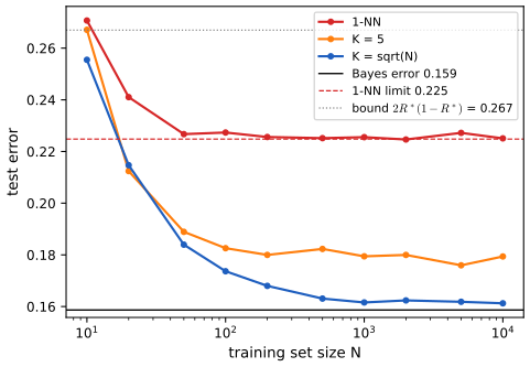
Numerical confirmation. Two equal-prior unit-covariance Gaussians in the plane whose means are 2 apart have \(R^*=\Phi(-1)=0.1587\); the exact limit by quadrature is \(R_{\rm 1NN}=0.2248\), below the bound \(2R^*(1-R^*)=0.2670\); simulated 1-NN error at \(N=10^4\) is \(0.2251\), and 5-NN and \(\sqrt N\)-NN converge towards \(0.18\) and \(0.161\). The multiclass pointwise inequality was also checked on random probability vectors.
16.1.1 Example
p. 548 Figure 16.1a shows \(K=5\) in the plane. Three of the five neighbours of the test point (the cross) have label 1 and two have label 0, so \(p(y=1\given\bm x,\mathcal D)=3/5\). With \(K=1\) the predictive distribution is a point mass on the label of the nearest neighbour, and the plane is partitioned into the Voronoi cells \(V(\bm x_n)=\{\bm x:\|\bm x-\bm x_n\|\le\|\bm x-\bm x_m\|\ \forall m\}\) (Figure 16.1b). Each cell is an intersection of half-planes \(\{\bm x:\|\bm x-\bm x_n\|^2\le\|\bm x-\bm x_m\|^2\}=\{2(\bm x_m-\bm x_n)^\T\bm x\le\|\bm x_m\|^2-\|\bm x_n\|^2\}\), hence a convex polytope. The prediction inside a cell is the label of its training point, so the training error is zero (provided no two identical inputs carry different labels), and the classifier usually overfits.
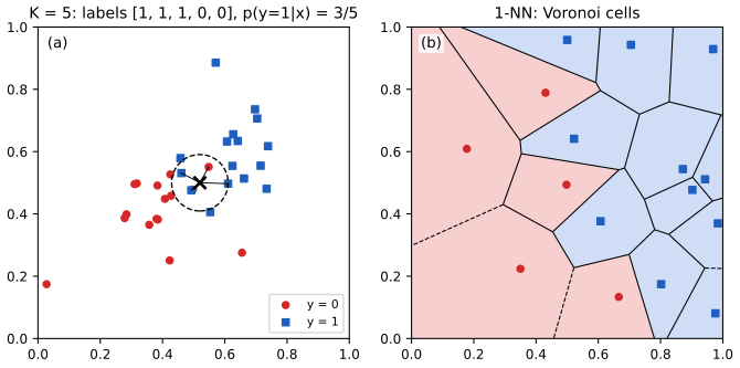
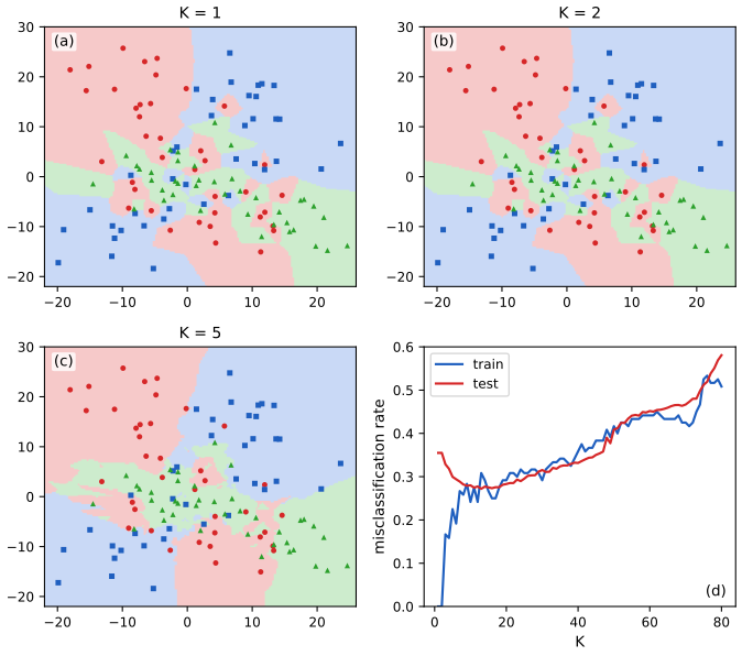
Figure 16.2 applies the classifier to a three-class problem. At \(K=1\) the decision regions are ragged and the training error is exactly 0; as \(K\) grows each prediction averages over a larger neighbourhood, so the boundaries smooth, the training error rises (underfitting) and the test error traces the familiar U shape (panel d). In my simulated version (each class a mixture of two Gaussians, 120 training points, 3000 test points) the test error falls from 0.355 at \(K=1\) to its minimum of 0.272 at \(K=13\) and then climbs back to 0.58 at \(K=80\), where the neighbourhood covers two thirds of the data.
16.1.2 The curse of dimensionality
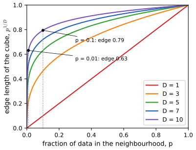
pp. 548–550 The main statistical weakness of KNN is high dimension. Volume grows exponentially with the dimension \(D\), so the closest of \(N\) points can be far away. To make this precise, take inputs uniform in the unit cube and suppose we estimate the class densities around \(\bm x\) by growing a hypercube around \(\bm x\) until it holds a fraction \(p\) of the data. Its expected edge length is \[ e_D(p)=p^{1/D}, \tag{Figure 16.3b} \] because a cube of edge \(s\) has volume \(s^D\). For \(D=10\): \(e_{10}(0.1)=0.79\) and \(e_{10}(0.01)=0.63\): to use only 1% of the data one must extend the cube across 63% of the range of every coordinate, so the neighbourhood is not local. There are two main remedies: assume a parametric form (so that distant data are informative), or learn a metric that only cares about a subset of the dimensions (Section 16.2).
Filling the gap 16.2: edge length, the distance to the nearest neighbour, distance concentration, and nuisance coordinates pp. 548–550, Figure 16.3
Derivation
(a) Edge length. If \(\bm X\sim\mathrm{Unif}[0,1]^D\) and a cube of edge \(s\) lies inside the unit cube, \(\Pr(\bm X\in\text{cube})=s^D\); setting it equal to \(p\) gives \(s=p^{1/D}\). For a query near the boundary the cube is clipped and holds a fraction at most \(s^D\), so the edge must be larger still: the formula is a lower bound for the cube needed. For fixed \(p\in(0,1)\), \(p^{1/D}=\exp(\ln p/D)\to1\) as \(D\to\infty\).
(b) Distance to the nearest neighbour. Let \(N\) points be uniform in the unit ball of \(\R^D\) and measure from the origin. A point lies within distance \(t\) with probability \(t^D\) (ratio of volumes), so the distance \(R_{(1)}\) to the closest point satisfies \(\Pr(R_{(1)}>t)=(1-t^D)^N\). Its median solves \((1-t^D)^N=\frac12\), that is \[ t_{\rm med}=\big(1-2^{-1/N}\big)^{1/D}. \] For \(N=500\), \(D=10\): \(t_{\rm med}=(0.00139)^{0.1}=0.52\), so the nearest neighbour is more than half-way to the boundary of the ball. (A simulation with \(N=30,D=3\) gives 0.286 against the formula's 0.284.)
(c) Distances concentrate. For independent uniform \(U,U'\), the variable \((U-U')^2\) has mean \(1/6\) and variance \(\E(U-U')^4-1/36=1/15-1/36=7/180\). For \(\bm X,\bm X'\) uniform in the cube, \(\|\bm X-\bm X'\|^2\) is a sum of \(D\) such terms, so it has mean \(D/6\) and relative standard deviation \(\sqrt{7/180}\cdot6/\sqrt D=1.18/\sqrt D\to0\). In high dimension all pairwise distances are nearly equal and "nearest" carries little information (Figure 16.S2b).
(d) Nuisance coordinates. Suppose the label depends only on the first two coordinates and the others (\(D-2\) of them) are noise. The squared Euclidean distance is the sum of an informative part and a noise part; the noise part has mean \((D-2)/6\) and standard deviation \(0.197\sqrt{D-2}\) between candidate neighbours. Once this fluctuation is larger than the spread in the informative part among the closest candidates (which is of order \(1/N\) in the plane), the ranking of neighbours is decided by noise and the KNN prediction degrades towards a random guess. A metric that ignores the noise coordinates removes the problem altogether (teal lines in Figure 16.S2a; the demonstration below).
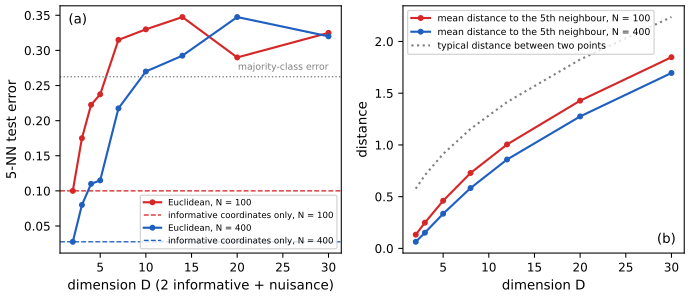
See also: the curse of dimensionality demo (Elements of Statistical Learning) and its nonparametric-estimation version.
16.1.3 Reducing the speed and memory requirements
p. 550 KNN stores every training example, and a naive query costs \(O(ND)\). Pruning heuristics remove points that do not affect the decision boundary (Section 17.4 of the book gives a principled sparse alternative). For speed the aim is to find the \(K\) nearest neighbours in time below \(O(N)\). Exact search is practical in low dimension (a k-d tree divides space into axis-parallel boxes by recursive median splits, and a query skips every box that cannot contain a point nearer than the best found so far), but its cost climbs to a full scan around \(D\approx10\); in higher dimension one settles for approximate neighbours, using space partitioning (trees, clustering with anchor points) or hashing. Locality-sensitive hashing (LSH) [GIM99] maps similar inputs to the same bucket with high probability; later methods learn the hash function. The library FAISS (Johnson, Douze and Jégou, 2017) provides exact and approximate nearest-neighbour search for dense vectors.
Filling the gap 16.3: why exact tree search degrades with the dimension, and why random-hyperplane hashing works p. 550, [GIM99]
Derivation
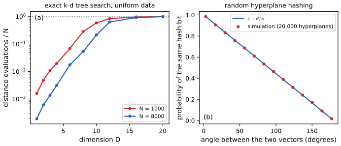
Cost of a k-d tree. After median splits to leaves of one point, the tree has \(N\) cells, and each coordinate has been split about \(\log_2N/D\) times along any root-to-leaf path. For a query \(\bm q\) with current best distance \(\rho\), the search must visit every cell that intersects the ball \(B(\bm q,\rho)\). A cell has typical width \(N^{-1/D}\) along each coordinate (\(N\) cells share the unit cube), while \(\rho\) is of order the nearest-neighbour distance, itself \(\asymp N^{-1/D}\) (the ball of radius \(\rho\) must hold about one point). The ball therefore crosses a splitting hyperplane in every coordinate, and the number of cells it meets is about \(2^D\): when \(N\lesssim2^D\) the search touches essentially all cells. This heuristic (the cost grows like \(\min\{N,2^D\}\)) is confirmed by Figure 16.S3a: for \(N=1000\) the fraction of distance evaluations reaches about 1 near \(D=12\) and for \(N=8000\) near \(D=16\) to 20, in line with \(2^{10}\approx10^3\) and \(2^{13}\approx8000\). The k-d tree used there is exact; it was compared with brute force.
Random-hyperplane hashing. Draw \(\bm g\sim\mathcal N(\bm0,\bm I_D)\) and set the hash bit \(h_{\bm g}(\bm x)=\sign(\bm g^\T\bm x)\). Claim: if \(\theta\in[0,\pi]\) is the angle between \(\bm x\) and \(\bm x'\), \(\Pr[h_{\bm g}(\bm x)=h_{\bm g}(\bm x')]=1-\theta/\pi\). Proof. Only the projection of \(\bm g\) on the plane spanned by \(\bm x,\bm x'\) matters; since the standard normal is rotation invariant, this projection is a standard normal in the plane and its direction \(\varphi\) is uniform on \([0,2\pi)\). In the plane write \(\bm x,\bm x'\) at angles \(\alpha,\alpha+\theta\). Then \(\bm g^\T\bm x\propto\cos(\varphi-\alpha)\) and \(\bm g^\T\bm x'\propto\cos(\varphi-\alpha-\theta)\); the signs differ exactly when \(\varphi\) lies in one of two arcs of length \(\theta\) (the directions for which the line \(\bm g^\perp\) separates \(\bm x\) from \(\bm x'\)). Hence \(\Pr[\text{differ}]=2\theta/(2\pi)=\theta/\pi\). \(\square\) Figure 16.S3b compares the formula with 20 000 simulated hyperplanes.
Amplification. With \(p=1-\theta/\pi\) per bit, concatenating \(k\) independent bits into one key collides with probability \(p^k\) and using \(L\) independent tables makes the pair a candidate with probability \(1-(1-p^k)^L\), an S-shaped function of \(p\) that is steep around \(p\approx L^{-1/k}\). Choosing \(k\) and \(L\) so that near pairs (\(\theta\) small) collide with high probability and far pairs with low probability gives sub-linear query time at the price of some missed neighbours, the guarantee of [GIM99].
16.1.4 Open set recognition
pp. 550–551 Everything so far assumed a closed world: a fixed set of classes. Many applications are open: a face recogniser may meet a person it has never seen. Novelty detection asks whether a new input \(\bm x_{t+1}\) belongs to a class unseen so far; if it does, the system may request a label and add the pair to the data set, which grows the label set (incremental, online or continual learning). Detecting inputs from an entirely unrelated distribution (a photo of a dog) is out-of-distribution (OOD) detection. In these settings only a few (sometimes one) examples per class are available, which is few-shot classification (Section 19.6). KNN is well suited: store the gallery, find the nearest stored example \(\bm x'\) to the new input, and decide whether \(\bm x'\) and \(\bm x_{t+1}\) are similar enough to be a match (face verification, re-identification); if not, declare the input novel. All the work is in the distance (Section 16.2). The same open-world assumption underlies entity resolution (do "John Smith" and "Jon Smith" refer to the same entity?) and multi-object tracking (is a new radar blip an existing object or a new one?), for which random finite sets give a mathematical framework (the book points to the work of Mahler and of Vo and co-authors).
Filling the gap 16.4: thresholding the nearest-exemplar distance is a density-level test pp. 550–551
Derivation
Statement. Let the gallery \(\bm X_1,\dots,\bm X_N\) be i.i.d. from a density \(p\) on \(\R^D\) that is continuous and positive at \(\bm x\), let \(r_N(\bm x)=\min_n\|\bm X_n-\bm x\|\) and \(v_D\) the volume of the unit ball. Then \(N v_D\,p(\bm x)\,r_N(\bm x)^D\) converges in distribution to an exponential random variable with mean 1.
Proof. \(\Pr(r_N>t)=(1-P(B(\bm x,t)))^N\) and \(P(B(\bm x,t))=p(\bm x)v_Dt^D(1+o(1))\) as \(t\to0\) by continuity. Put \(t^D=u/(Nv_Dp(\bm x))\): \(\Pr(Nv_Dp\,r_N^D>u)=\big(1-\tfrac uN(1+o(1))\big)^N\to e^{-u}\). \(\square\)
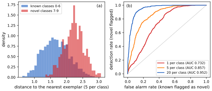
Consequence. For a query that comes from a known class, the nearest-exemplar distance is of order \((Nv_Dp(\bm x))^{-1/D}\): small where the gallery is dense, large where it is sparse. Flagging the query as novel when \(r_N(\bm x)>\tau\) is therefore the same as declaring it novel when the gallery density at \(\bm x\) is below the level \(c/(Nv_D\tau^D)\) (an estimate of a density level set), and the false-alarm probability for a known \(\bm x\) is \(\Pr(r_N>\tau)=(1-P(B(\bm x,\tau)))^N\le e^{-NP(B(\bm x,\tau))}\), which goes to 0 exponentially fast in the gallery size whenever \(P(B(\bm x,\tau))>0\). A query from a genuinely new class lying at distance more than \(\tau\) from all stored examples is flagged with probability 1. The rule fails exactly when the new class overlaps the known ones, the difficulty the book mentions for new faces that look like known ones.
Numerical illustration (Figure 16.S6). On the digits data the gallery holds the first \(g\) images of each of the classes 0 to 6, and the queries are the other known-class images and all images of classes 7, 8, 9. The area under the ROC curve of the nearest-exemplar distance for novelty detection is 0.73, 0.86 and 0.95 for \(g=1,5,20\) per class, and the closed-set 1-NN accuracy on the known classes is 0.77, 0.92 and 0.97: both improve with the gallery, as the statement predicts.
The key ingredient of every one of these tasks is the (dis)similarity measure itself, the topic of Section 16.2.
16.2 Learning distance metrics
pp. 551–552 A good "semantic" distance \(d(\bm x,\bm x')\in\R_+\), or equivalently a similarity \(s(\bm x,\bm x')\), is essential for nearest-neighbour classification, for self-supervised learning (Section 19.2.4.4), for similarity-based clustering (Section 21.5), for content-based retrieval and for visual tracking. On \(\mathcal X=\R^D\) the common choice is the Mahalanobis distance (16.3); Section 16.2.1 learns the matrix \(\bm M\), directly as a convex problem or indirectly through a linear map \(\bm W\) with \(\bm M=\bm W^\T\bm W\). For high-dimensional or structured inputs it is better to first learn a nonlinear embedding \(\bm e=f(\bm x)\) and measure distances in embedding space; when \(f\) is a deep network this is deep metric learning (DML, Section 16.2.2).
16.2.1 Linear and convex methods
16.2.1.1 Large margin nearest neighbors
p. 552 LMNN [WS09] learns \(\bm M\) so that a nearest-neighbour classifier works well. For every point \(i\) fix a set \(\mathcal N_i\) of target neighbours (usually the \(K\) nearest points of the same class in Euclidean distance). The pull term makes each point close to its targets, \[ L_{\rm pull}(\bm M)=\sum_{i=1}^N\sum_{j\in\mathcal N_i}d_{\bm M}(\bm x_i,\bm x_j)^2, \tag{16.4} \] and the push term forces every point of another class (an impostor) to be farther from \(i\) than each target neighbour by a margin \(m\ge0\), \[ L_{\rm push}(\bm M)=\sum_{i=1}^N\sum_{j\in\mathcal N_i}\sum_{l=1}^N\ind(y_i\ne y_l)\,\big[m+d_{\bm M}(\bm x_i,\bm x_j)^2-d_{\bm M}(\bm x_i,\bm x_l)^2\big]_+. \tag{16.5} \] The objective is \(L(\bm M)=(1-\lambda)L_{\rm pull}+\lambda L_{\rm push}\) with \(0<\lambda<1\). It is convex over the convex cone of positive semi-definite matrices and can be minimised by semi-definite programming. Alternatively write \(\bm M=\bm W^\T\bm W\) and minimise over \(\bm W\) by unconstrained gradient methods: this is no longer convex, but allows a low-dimensional map \(\bm W\in\R^{L\times D}\), \(L<D\). Evaluating (16.5) naively costs \(O(KN^2)\) (the book writes \(O(N^3)\)); the speed-up tricks of Section 16.2.5 apply.
Filling the gap 16.5: LMNN is a convex program; the gradient and a projected-gradient solver p. 552, (16.4), (16.5)
Derivation
Linearity in \(\bm M\). With \(\bm C_{ij}=(\bm x_i-\bm x_j)(\bm x_i-\bm x_j)^\T\), \(d_{\bm M}(\bm x_i,\bm x_j)^2=(\bm x_i-\bm x_j)^\T\bm M(\bm x_i-\bm x_j)=\Tr(\bm M\bm C_{ij})\), a linear function of \(\bm M\). Hence \(L_{\rm pull}\) is linear and each hinge \([m+\Tr(\bm M\bm C_{ij})-\Tr(\bm M\bm C_{il})]_+\) is the positive part of an affine function of \(\bm M\), which is convex. A nonnegative combination of convex functions is convex, so \(L\) is convex on the convex cone \(\mathbb S_+^D\) of positive semi-definite matrices. Introducing a slack variable \(\xi_{ijl}\ge0\) for every hinge turns the problem into the semi-definite program: minimise \((1-\lambda)\sum\Tr(\bm M\bm C_{ij})+\lambda\sum\xi_{ijl}\) subject to \(\xi_{ijl}\ge m+\Tr(\bm M(\bm C_{ij}-\bm C_{il}))\), \(\xi_{ijl}\ge0\), \(\bm M\succeq0\).
Gradient. Since \(\partial\Tr(\bm M\bm C)/\partial\bm M=\bm C\), a (sub)gradient is \[ \nabla L(\bm M)=(1-\lambda)\sum_{i,j\in\mathcal N_i}\bm C_{ij}+\lambda\sum_{(i,j,l)\in\mathcal A}(\bm C_{ij}-\bm C_{il}), \] where \(\mathcal A\) is the set of active triples (those with \(y_l\ne y_i\) and positive hinge). A finite-difference test along random symmetric directions confirmed this formula.
Projected gradient descent. Iterate \(\bm M\leftarrow\Pi_+(\bm M-\eta\nabla L(\bm M))\), where \(\Pi_+\) is the Frobenius-norm projection on \(\mathbb S_+^D\). Claim: for symmetric \(\bm A=\bm V\bm\Lambda\bm V^\T\), \(\Pi_+(\bm A)=\bm V\bm\Lambda_+\bm V^\T\) with \(\bm\Lambda_+=\diag(\max(\lambda_i,0))\). Proof: for any \(\bm B\succeq0\), \(\|\bm A-\bm B\|_F^2=\|\bm\Lambda-\bm V^\T\bm B\bm V\|_F^2\ge\sum_i(\lambda_i-b_{ii})^2\ge\sum_{\lambda_i<0}\lambda_i^2\) with \(b_{ii}\ge0\) the diagonal of \(\bm V^\T\bm B\bm V\succeq0\), and \(\bm B=\bm V\bm\Lambda_+\bm V^\T\) attains the bound. \(\square\) With backtracking on \(\eta\) (halve until the objective does not increase) the objective trace is monotone; since the problem is convex, any point where the projected gradient step leaves \(\bm M\) unchanged is a global minimiser. Cholesky or eigendecomposition then gives \(\bm W\) with \(\bm M=\bm W^\T\bm W\), and \(d_{\bm M}(\bm x,\bm x')=\|\bm W(\bm x-\bm x')\|\). The low-rank map (\(L<D\)) is a rank constraint, hence not convex.
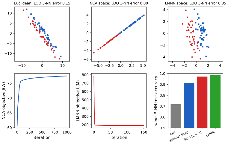
Numerical confirmation. The objective trace was monotone and the learned matrix positive semi-definite. On the toy problem of Figure 16.S4 (80 points, a class direction tilted by 35 degrees and a large spread across it) the leave-one-out 3-NN error drops from 0.150 (Euclidean) to 0.050 (LMNN, \(K=3\) targets, \(\lambda=0.5\), \(m=1\)); on the wine data (13 features, 60% for training and 71 test points) the 5-NN test accuracy is 0.72 on the raw features, 0.92 after standardisation and 0.99 after LMNN on the standardised features. One test point is 1.4 percent, so the gaps between the learned metrics (NCA 0.97, LMNN 0.99) are within the noise of one split.
16.2.1.2 Neighborhood components analysis
pp. 552–553 NCA [Gol+05] also learns a linear map \(\bm W\) with \(\bm M=\bm W^\T\bm W\), but replaces the hard neighbour choice by a soft one. Point \(i\) picks point \(j\neq i\) as its neighbour with the softmax probability \[ p_{ij}^{\bm W}=\frac{\exp(-\|\bm W\bm x_i-\bm W\bm x_j\|_2^2)}{\sum_{l\ne i}\exp(-\|\bm W\bm x_i-\bm W\bm x_l\|_2^2)}. \tag{16.6} \] (This is a supervised version of stochastic neighbour embedding, Section 20.4.10.1.) The expected number of points that a 1-NN rule with this stochastic choice classifies correctly (leave one out) is \(J(\bm W)=\sum_{i=1}^N\sum_{j\ne i:\,y_j=y_i}p_{ij}^{\bm W}\), and \(L(\bm W)=1-J(\bm W)/N\) is the corresponding leave-one-out error. Both are smooth, so gradient methods apply.
Filling the gap 16.6: the gradient of the NCA objective, invariances, and the behaviour of the optimum p. 553, (16.6)
Derivation
Gradient. Write \(\bm x_{ij}=\bm x_i-\bm x_j\), \(d_{ij}=\|\bm W\bm x_{ij}\|^2\), \(\mathcal C_i=\{j\ne i:y_j=y_i\}\) and \(p_i=\sum_{j\in\mathcal C_i}p_{ij}\). Since \(\partial d_{ij}/\partial\bm W=2\bm W\bm x_{ij}\bm x_{ij}^\T\) and \(p_{ij}=e^{-d_{ij}}/\sum_le^{-d_{il}}\), \[ \frac{\partial p_{ij}}{\partial\bm W}=p_{ij}\Big(-\frac{\partial d_{ij}}{\partial\bm W}+\sum_{k\ne i}p_{ik}\frac{\partial d_{ik}}{\partial\bm W}\Big)=2p_{ij}\bm W\Big(-\bm x_{ij}\bm x_{ij}^\T+\sum_{k\ne i}p_{ik}\bm x_{ik}\bm x_{ik}^\T\Big). \] Summing over \(j\in\mathcal C_i\) and \(i\), \[ \frac{\partial J}{\partial\bm W}=2\bm W\sum_{i=1}^N\Big(p_i\sum_{k\ne i}p_{ik}\bm x_{ik}\bm x_{ik}^\T-\sum_{j\in\mathcal C_i}p_{ij}\bm x_{ij}\bm x_{ij}^\T\Big). \] The first term pulls \(i\) away from everything in proportion to how likely it is to be chosen, the second pulls it towards its own class. A finite-difference test agreed with this gradient to \(10^{-9}\).
Invariances. \(J(\bm Q\bm W)=J(\bm W)\) for every orthogonal \(\bm Q\), since the distances \(\|\bm W\bm x_{ij}\|\) depend on \(\bm W\) only through \(\bm W^\T\bm W\). Hence the optimum is a set of maps, not a single map, and plots of the learned space may appear rotated.
Behaviour. \(0\le J\le N\). If every point's nearest neighbours (in the final metric) are of its own class, \(J\) can be increased by scaling \(\bm W\) up, which sharpens the softmax; on well-separated data the optimum is at infinity, which is why NCA is run for a limited number of iterations or with a regulariser. The iteration \(\bm W\leftarrow\bm W+\eta\,\partial J/\partial\bm W\) with the small fixed step \(\eta=0.002\) used in the demonstration increases \(J\) at every step on the toy problem (Figure 16.S4), from \(J=60.7\) to \(77.4\) of at most 80, and the learned map has singular values \((3.60,0.00)\): it is rank one, keeping only the informative direction. Because \(J\) is not concave, gradient ascent finds a local maximum in general.
See also: a classical learned metric, discriminant adaptive nearest neighbours, and the adaptive nearest-neighbour methods of Elements of Statistical Learning.
16.2.1.3 Latent coincidence analysis
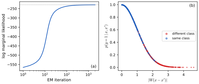
p. 553 LCA [DS12] is a conditional latent-variable model for a pair \((\bm x,\bm x')\) and a label \(y\in\{0,1\}\) saying whether they are similar (for example, of the same class). Each input is mapped to a low-dimensional latent point by a noisy linear map, \(p(\bm z\given\bm x)=\mathcal N(\bm z\given\bm W\bm x,\sigma^2\bm I)\) and \(p(\bm z'\given\bm x')=\mathcal N(\bm z'\given\bm W\bm x',\sigma^2\bm I)\), with \(\bm W\in\R^{L\times D}\) (compare factor analysis, Section 20.2). The two points coincide with probability \(p(y=1\given\bm z,\bm z')=\exp(-\|\bm z-\bm z'\|^2/(2\kappa^2))\) (see the note on the book at the end: the norm must be squared). The log marginal likelihood \(\ell(\bm W,\sigma^2,\kappa^2)=\sum_n\log p(y_n\given\bm x_n,\bm x_n')\) is maximised by EM (Section 8.7.2): the E step needs the posterior of \((\bm z,\bm z')\) given \((\bm x,\bm x',y)\), in closed form, and the M step is a weighted least-squares problem. EM increases \(\ell\) monotonically and needs no step size, unlike the gradient methods of NCA. The scale \(\kappa=1\) can be fixed without loss of generality, since it only rescales \(\bm W\).
Filling the gap 16.7: the LCA marginal likelihood, the E step in closed form, the M step, and monotonicity p. 553, [DS12]
Derivation
Change of variables. Let \(\bm u=\bm z-\bm z'\) and \(\bm v=\bm z+\bm z'\), \(\bm d=\bm x-\bm x'\) and \(\bm s=\bm x+\bm x'\). Given the inputs, \(\bm z\) and \(\bm z'\) are independent Gaussians with the same variance, so \(\bm u\sim\mathcal N(\bm W\bm d,2\sigma^2\bm I)\) and \(\bm v\sim\mathcal N(\bm W\bm s,2\sigma^2\bm I)\) are independent (their covariance is \(\sigma^2\bm I-\sigma^2\bm I=\bm0\)). The label depends on \(\bm u\) only.
Marginal likelihood. Put \(\bm m=\bm W\bm d\) and \(\tau=2\sigma^2\). In one coordinate, completing the square, \[ \int\mathcal N(u\given m,\tau)\,e^{-u^2/(2\kappa^2)}\,\d u=\sqrt{\frac{\kappa^2}{\kappa^2+\tau}}\;\exp\Big(-\frac{m^2}{2(\kappa^2+\tau)}\Big), \] so over \(L\) coordinates \[ A:=p(y=1\given\bm x,\bm x')=\Big(1+\frac{2\sigma^2}{\kappa^2}\Big)^{-L/2}\exp\Big(-\frac{\|\bm W(\bm x-\bm x')\|^2}{2(\kappa^2+2\sigma^2)}\Big), \] and \(p(y=0\given\bm x,\bm x')=1-A\). Replacing \((\bm W,\sigma^2,\kappa^2)\) by \((c\bm W,c^2\sigma^2,c^2\kappa^2)\) leaves \(A\) unchanged, which justifies \(\kappa=1\). A Monte Carlo check (\(10^6\) draws) and a one-dimensional quadrature agreed with \(A\).
E step. Multiplying the prior density of \(\bm u\) by the likelihood \(e^{-\|\bm u\|^2/(2\kappa^2)}\) gives the unnormalised density \(A\,\mathcal N(\bm u\given\bm m_1,s^2\bm I)\) with \(s^2=(\frac1{2\sigma^2}+\frac1{\kappa^2})^{-1}\) and \(\bm m_1=\frac{s^2}{2\sigma^2}\bm m\) (the normaliser is \(A\) by the previous display). So \[ p(\bm u\given y=1)=\mathcal N(\bm m_1,s^2\bm I),\qquad p(\bm u\given y=0)=\frac{\mathcal N(\bm m,2\sigma^2\bm I)-A\,\mathcal N(\bm m_1,s^2\bm I)}{1-A}, \] a signed mixture, since \(1-e^{-\|\bm u\|^2/2\kappa^2}\) multiplies the prior. The moments needed are \(\E[\bm u\given y=1]=\bm m_1\), \(\E[\bm u\given y=0]=(\bm m-A\bm m_1)/(1-A)\), \(\E[\|\bm u-\bm m\|^2\given y=1]=Ls^2+\|\bm m_1-\bm m\|^2\) and \(\E[\|\bm u-\bm m\|^2\given y=0]=\big(2\sigma^2L-A(Ls^2+\|\bm m_1-\bm m\|^2)\big)/(1-A)\); the posterior of \(\bm v\) equals its prior. (All four were verified by one-dimensional quadrature.)
M step. The complete-data log likelihood is \(\log p(\bm z\given\bm x)+\log p(\bm z'\given\bm x')+\log p(y\given\bm z,\bm z')\), and the last term does not involve \((\bm W,\sigma^2)\). With \(S_n=\E\|\bm z_n-\bm W\bm x_n\|^2+\E\|\bm z_n'-\bm W\bm x_n'\|^2\), \[ Q(\bm W,\sigma^2)=-\frac1{2\sigma^2}\sum_nS_n-NL\log(2\pi\sigma^2)+\const. \] Setting \(\partial Q/\partial\bm W=0\) gives the weighted least-squares solution \(\bm W=\big(\sum_n\E[\bm z_n]\bm x_n^\T+\E[\bm z_n']\bm x_n'^\T\big)\big(\sum_n\bm x_n\bm x_n^\T+\bm x_n'\bm x_n'^\T\big)^{-1}\) with \(\E\bm z=\frac12(\bm W_{\rm old}\bm s+\E\bm u)\), \(\E\bm z'=\frac12(\bm W_{\rm old}\bm s-\E\bm u)\), and \(\partial Q/\partial\sigma^2=0\) gives \(\sigma^2=\sum_nS_n/(2NL)\). By the parallelogram identity \(\|\bm a\|^2+\|\bm b\|^2=\frac12(\|\bm a+\bm b\|^2+\|\bm a-\bm b\|^2)\), \(S_n=\frac12\big(\E\|\bm u-\bm W\bm d\|^2+\E\|\bm v-\bm W\bm s\|^2\big)\), which only needs the moments above.
Monotonicity. For any parameters \(\bm\theta,\bm\theta_t\), with latent variable \(\bm\zeta\), \(\ell(\bm\theta)-\ell(\bm\theta_t)=\big[Q(\bm\theta\given\bm\theta_t)-Q(\bm\theta_t\given\bm\theta_t)\big]+\KL\big(p(\bm\zeta\given\cdot,\bm\theta_t)\,\|\,p(\bm\zeta\given\cdot,\bm\theta)\big)\ge Q(\bm\theta\given\bm\theta_t)-Q(\bm\theta_t\given\bm\theta_t)\) (Gibbs' inequality), so any \(\bm\theta\) that increases \(Q\), in particular the M-step maximiser, increases \(\ell\). \(\square\)
Numerical confirmation. On 800 random pairs from the toy problem (similar = same class), one latent dimension, the log likelihood increased at every one of 2000 iterations (Figure 16.S5a) and the learned \(\bm W\) has \(|\cos|=1.0000\) with the informative direction. The likelihood approaches its supremum, found by direct maximisation (dotted line), slowly: on these data the supremum is approached as \(\sigma^2\to0\) (the final value is \(\sigma^2=0.003\)), where EM is slow; the log likelihood is \(-229.74\) at iteration 2000 against \(-229.50\) at the supremum.
16.2.2 Deep metric learning
p. 554 For high-dimensional or structured inputs, learn an embedding \(\bm e=f(\bm x;\bm\theta)\in\R^L\) that keeps the relevant semantic aspects, normalise it, \(\hat{\bm e}=\bm e/\|\bm e\|_2\) (so all points lie on a hypersphere), and measure similarity by the normalised squared Euclidean distance or the cosine similarity \[ d(\bm x_i,\bm x_j;\bm\theta)=\|\hat{\bm e}_i-\hat{\bm e}_j\|_2^2,\qquad\hat{\bm e}_i^\T\hat{\bm e}_j, \tag{16.7, 16.8} \] which are linked by \(\|\hat{\bm e}_i-\hat{\bm e}_j\|_2^2=\hat{\bm e}_i^\T\hat{\bm e}_i-2\hat{\bm e}_i^\T\hat{\bm e}_j+\hat{\bm e}_j^\T\hat{\bm e}_j=2-2\hat{\bm e}_i^\T\hat{\bm e}_j\) (16.9), since unit vectors have \(\hat{\bm e}^\T\hat{\bm e}=1\). The cosine measures the angle between the embeddings. With a labelled data set one forms the set of similar pairs \(\mathcal S=\{(i,j):y_i=y_j\}\) and wants \(\bm x_i\) and \(\bm x_j\) close in embedding space when \((i,j)\in\mathcal S\) and \(\bm x_i,\bm x_k\) far when \((i,k)\notin\mathcal S\). The methods also work without class labels as long as another rule defines similar pairs, as in self-supervised learning (Section 19.2.4.3), where data augmentation creates them. A caution from the book: many recent DML methods are not as good as they claim [MBL20; Rot+20], because the comparisons were improper; the book therefore focuses on older, simpler and more robust losses.
16.2.3 Classification losses
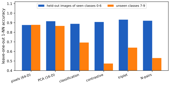
p. 554 With \(C\) labelled classes one can fit a classifier in \(O(NC)\) time and reuse a hidden layer as the embedding (the second-to-last layer generalises better to new classes than the final one). This is simple and scalable, but it only learns to put examples on the correct side of a decision boundary, not necessarily close to similar examples and far from dissimilar ones, and it needs labels. In the experiment of Figure 16.S7 below it is the best of the learned embeddings on classes that were not seen in training.
16.2.4 Ranking losses
pp. 555–556 Ranking losses ask only that similar examples be closer than dissimilar ones.
16.2.4.1 Pairwise (contrastive) loss and Siamese networks
The contrastive loss [CHL05] of a pair is \[ L(\bm\theta;\bm x_i,\bm x_j)=\ind(y_i=y_j)\,d(\bm x_i,\bm x_j)^2+\ind(y_i\ne y_j)\,[m-d(\bm x_i,\bm x_j)]_+^2, \tag{16.10} \] with margin \(m>0\): similar pairs are pulled together, and dissimilar pairs are pushed apart until they are at least \(m\) away, after which they cost nothing. The same feature extractor \(f(\cdot;\bm\theta)\) embeds both inputs, hence the name Siamese network (Figure 16.5a, a hand-drawn architecture sketch). Minimising over all pairs naively costs \(O(N^2)\).
16.2.4.2 Triplet loss
In the pairwise loss the treatment of positive pairs is independent of the negative pairs, so their magnitudes may be incomparable. The triplet loss [SKP15] uses an anchor \(\bm x_i\), a positive \(\bm x_i^+\) and a negative \(\bm x_i^-\): \[ L(\bm\theta;\bm x_i,\bm x_i^+,\bm x_i^-)=\big[d_{\bm\theta}(\bm x_i,\bm x_i^+)^2-d_{\bm\theta}(\bm x_i,\bm x_i^-)^2+m\big]_+, \tag{16.11} \] so the anchor-positive distance must be smaller than the anchor-negative distance by a margin (a triplet network, Figure 16.5b). Over all triples this costs \(O(N^3)\); in practice minibatches are used, chosen to contain at least one positive and one negative for the anchor, and the speed-ups of Section 16.2.5 apply.
16.2.4.3 N-pairs loss
The triplet loss compares an anchor with only one negative at a time, which may be a weak signal. The N-pairs loss [Soh16] builds a multi-class problem with \(N-1\) negatives \(\{\bm x_k^-\}\) and one positive for every anchor: \[ L=\log\Big(1+\sum_{k=1}^{N-1}\exp\big(\hat{\bm e}_{\bm\theta}(\bm x)^\T\hat{\bm e}_{\bm\theta}(\bm x_k^-)-\hat{\bm e}_{\bm\theta}(\bm x)^\T\hat{\bm e}_{\bm\theta}(\bm x^+)\big)\Big)=-\log\frac{\exp(\hat{\bm e}(\bm x)^\T\hat{\bm e}(\bm x^+))}{\exp(\hat{\bm e}(\bm x)^\T\hat{\bm e}(\bm x^+))+\sum_{k}\exp(\hat{\bm e}(\bm x)^\T\hat{\bm e}(\bm x_k^-))}. \tag{16.12, 16.13} \] It coincides with the InfoNCE loss of the CPC paper [OLV18]; scaling the similarities by a temperature gives the NT-Xent loss of [Che+20a] (the temperature scales the radius of the hypersphere). With one negative (\(N=2\)) it reduces to the logistic loss \[ L=\log\big(1+\exp(\hat{\bm e}(\bm x)^\T\hat{\bm e}(\bm x^-)-\hat{\bm e}(\bm x)^\T\hat{\bm e}(\bm x^+))\big), \tag{16.14} \] to be compared with the triplet margin loss at \(m=1\), \(\max(0,\hat{\bm e}(\bm x)^\T\hat{\bm e}(\bm x^-)-\hat{\bm e}(\bm x)^\T\hat{\bm e}(\bm x^+)+1)\) (16.15); the two functions are compared in Figure 4.2 of the book.
Filling the gap 16.8: N-pairs = InfoNCE = softmax cross entropy, the logistic limit, the temperature limit, and the gradient p. 556, (16.12)–(16.15)
Derivation
Write \(s_+=\hat{\bm e}(\bm x)^\T\hat{\bm e}(\bm x^+)\) and \(s_k=\hat{\bm e}(\bm x)^\T\hat{\bm e}(\bm x_k^-)\).
(a) (16.12) = (16.13). \(1+\sum_ke^{s_k-s_+}=\big(e^{s_+}+\sum_ke^{s_k}\big)/e^{s_+}\); take the log. The loss is the cross entropy of the softmax over the \(N\) candidates \(\{\bm x^+,\bm x_1^-,\dots,\bm x_{N-1}^-\}\) for the label "the positive": a multi-class classification problem in which the anchor must identify its partner.
(b) \(N=2\): (16.14), and the comparison with the hinge (16.15). With one negative the sum has one term, giving \(\log(1+e^{s_1-s_+})\). In terms of the margin variable \(z=s_1-s_+\) the two losses are \(\ell_{\rm log}(z)=\log(1+e^z)\) and \(\ell_{\rm hinge}(z)=[z+1]_+\). Both are convex and both are upper bounds of the 0-1 loss \(\ind(z\ge0)\) once the logistic loss is divided by \(\log2\): \([z+1]_+\ge\ind(z\ge0)\) because \([z+1]_+\ge1\) for \(z\ge0\), and \(\log(1+e^z)/\log2\ge\ind(z\ge0)\) because it equals 1 at \(z=0\) and increases. Moreover \([z]_+\le\log(1+e^z)\le[z]_++\log2\), so the logistic loss is a smooth version of the rectifier. Unlike the hinge it never reaches 0, so it keeps pushing easy examples apart (with exponentially decaying force).
(c) The temperature limit. With temperature \(\tau\), \(L_\tau=\log\big(1+\sum_k\exp((s_k-s_+)/\tau)\big)\) is the log-sum-exp of the \(N\) numbers \(0\) and \((s_k-s_+)/\tau\). For any numbers, \(\max_ia_i\le\lse(a)\le\max_ia_i+\log N\). Hence \[ \max\big(0,\max_k(s_k-s_+)\big)\;\le\;\tau L_\tau\;\le\;\max\big(0,\max_k(s_k-s_+)\big)+\tau\log N. \] As \(\tau\to0\), \(\tau L_\tau\) tends to the hinge loss with margin 0 on the hardest negative: only the most similar negative matters. For large \(\tau\) the loss averages over all negatives. The temperature thus interpolates between hardest-negative training and uniform treatment of the negatives. (Checked numerically for \(\tau=0.1,0.02,0.005\).)
(d) The gradient. Let \(\pi_+=e^{s_+/\tau}/Z\) and \(\pi_k=e^{s_k/\tau}/Z\) with \(Z=e^{s_+/\tau}+\sum_ke^{s_k/\tau}\). Since \(L=-s_+/\tau+\log Z\), \[ \frac{\partial L}{\partial\hat{\bm e}(\bm x)}=\frac1\tau\Big(\pi_+\hat{\bm e}(\bm x^+)+\sum_k\pi_k\hat{\bm e}(\bm x_k^-)-\hat{\bm e}(\bm x^+)\Big)=\frac1\tau\Big(\sum_k\pi_k\hat{\bm e}(\bm x_k^-)-(1-\pi_+)\hat{\bm e}(\bm x^+)\Big). \] Descent moves the anchor towards the positive and away from the negatives, each with a weight equal to its softmax probability: hard negatives (large \(s_k\)) get exponentially larger weights, an implicit form of the hard-negative mining of Section 16.2.5.1. The gradient with respect to the unnormalised \(\bm e\) is this vector multiplied by \((\bm I-\hat{\bm e}\hat{\bm e}^\T)/\|\bm e\|\). (A finite-difference check agreed to \(10^{-8}\).)
16.2.5 Speeding up ranking loss optimization
pp. 556–559 The main disadvantage of ranking losses is the \(O(N^2)\) or \(O(N^3)\) cost of comparing all pairs or triples.
16.2.5.1 Mining techniques
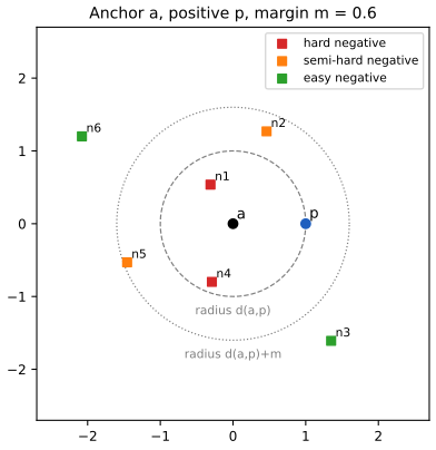
Most negatives are uninformative (they incur zero loss), so one can focus on hard negatives: for an anchor \(a\) with nearest positive \(p\), a negative \(n\) is hard if \(d(\bm x_a,\bm x_n)<d(\bm x_a,\bm x_p)\) and \(y_n\ne y_a\). Because an anchor may have no hard negative, the pool is widened to semi-hard negatives, for which \[ d(\bm x_a,\bm x_p)<d(\bm x_a,\bm x_n)<d(\bm x_a,\bm x_p)+m, \tag{16.16} \] the choice of Google's FaceNet [SKP15], which learns a face embedding. In practice hard negatives are chosen within the minibatch, which therefore needs to be large enough to be diverse, or a separate process keeps updating a candidate set as the metric evolves.
Filling the gap 16.9: easy, semi-hard and hard negatives and the loss they incur pp. 556–557, (16.11), (16.16), Figure 16.6a
Derivation
For an anchor-positive distance \(d_p=d(\bm x_a,\bm x_p)\), a negative at distance \(d_n\) and margin \(m\), define the hinge in distances \(\ell=[d_p-d_n+m]_+\). Then:
- easy (\(d_n\ge d_p+m\)): \(\ell=0\), no gradient, the negative is already far enough;
- semi-hard (\(d_p<d_n<d_p+m\)): \(0<\ell<m\);
- hard (\(d_n\le d_p\)): \(\ell\ge m\), the largest losses and gradients.
(Checked on 2000 random triples.) A caveat the book does not mention. The loss (16.11) is written with squared distances, \([d_p^2-d_n^2+m]_+\), which vanishes iff \(d_n^2\ge d_p^2+m\), and not iff \(d_n\ge d_p+m\). The taxonomy (16.16) and Figure 16.6a refer to the unsquared distances, so it classifies negatives exactly only for the unsquared hinge. For example with \(d_p=1\), \(d_n=1.2\), \(m=0.3\) the negative is semi-hard by (16.16) but the squared loss is \([1-1.44+0.3]_+=0\). Figure 16.6 therefore prints the unsquared hinge.
Why mining pays off. With \(N\) points in \(C\) balanced classes the number of valid triples is \(N(N/C-1)\cdot N(C-1)/C=O(N^3/C)\). Restricting each anchor-positive pair to its semi-hard or hard negatives, which are a small fraction once training has progressed, leaves \(O(N^2)\) or fewer terms with non-zero loss. Hardest-negative mining can be unstable early in training (outliers and mislabelled points are always hardest), which is the reason [SKP15] prefer semi-hard negatives.
16.2.5.2 Proxy methods
p. 557 Even with mining the triplet loss is expensive; ideally the cost is \(O(N)\) like classification. The proxy method of [MA+17] measures the distance between each anchor and a set of \(P\) proxies that represent the classes, rather than between examples. The proxies are learned online as the metric changes; the procedure takes \(O(NP^2)\) time with \(P\sim C\). The soft triple loss [Qia+19] represents each class with several prototypes while keeping the linear cost.
16.2.5.3 Optimizing an upper bound
pp. 557–559 [Do+19] define one fixed proxy (a centroid \(\bm c_m\)) per class and use distances to the proxies as an upper bound on the triplet loss without margin, \(\ell_t(\bm x_i,\bm x_j,\bm x_k)=\|\hat{\bm e}_i-\hat{\bm e}_j\|-\|\hat{\bm e}_i-\hat{\bm e}_k\|\) (16.17). The triangle inequalities \[ \|\hat{\bm e}_i-\hat{\bm e}_j\|\le\|\hat{\bm e}_i-\bm c_{y_i}\|+\|\hat{\bm e}_j-\bm c_{y_i}\|,\qquad\|\hat{\bm e}_i-\hat{\bm e}_k\|\ge\|\hat{\bm e}_i-\bm c_{y_k}\|-\|\hat{\bm e}_k-\bm c_{y_k}\| \tag{16.18, 16.19} \] give, for \(y_i=y_j\ne y_k\), \[ \ell_t\le\ell_u:=\|\hat{\bm e}_i-\bm c_{y_i}\|-\|\hat{\bm e}_i-\bm c_{y_k}\|+\|\hat{\bm e}_j-\bm c_{y_i}\|+\|\hat{\bm e}_k-\bm c_{y_k}\|, \tag{16.20} \] and, summing over all triples, \(L_t\le L_u=C'\sum_{i=1}^N\big[\|\hat{\bm e}_i-\bm c_{y_i}\|-\frac1{3(C-1)}\sum_{m\ne y_i}\|\hat{\bm e}_i-\bm c_m\|\big]\) (16.21, 16.22) with \(C'=3(C-1)(\frac NC-1)\frac NC\), for a balanced data set. \(L_u\) costs \(O(NC)\). The book states \(0\le L_t-L_u\le\frac{N^3}{C^2}K\); the sign is reversed (see the gap box). To make the bound tight the centroids should be far apart and equidistant, which one-hot vectors achieve (orthogonal unit vectors at distance \(\sqrt2\)); this assumes an embedding of dimension \(L=C\). Two fixes for \(L\ne C\): add a linear projection layer after training, or sample many points uniformly on the \(L\)-sphere (normalise Gaussian vectors [Mar72]) and run K-means with \(K=C\) (Section 21.3); [Do+19] report similar results. Finally [Rot+20] show that performance on retrieval tasks improves with the ratio \(\pi_{\rm intra}/\pi_{\rm inter}\) of the average intra-class distance, \(\pi_{\rm intra}=\frac1{Z_{\rm intra}}\sum_c\sum_{i\ne j:y_i=y_j=c}d(\bm x_i,\bm x_j)\) (16.23), to the average inter-class distance between class means \(\bm\mu_c=\frac1{Z_c}\sum_{i:y_i=c}\hat{\bm e}_i\), \(\pi_{\rm inter}=\frac1{Z_{\rm inter}}\sum_{c,c'}d(\bm\mu_c,\bm\mu_{c'})\) (16.24): keep the centroids far apart and do not let examples collapse onto their centroid, a term the bound of [Do+19] does not capture.
Filling the gap 16.10: the proxy bound, its closed form (16.22), the sign of the gap, and when it is tight pp. 557–558, (16.17)–(16.22)
Derivation
The bound. Add (16.18) and the rearranged (16.19), \(-\|\hat{\bm e}_i-\hat{\bm e}_k\|\le-\|\hat{\bm e}_i-\bm c_{y_k}\|+\|\hat{\bm e}_k-\bm c_{y_k}\|\), and use \(y_j=y_i\): this is (16.20). The slacks are \(\sigma_1=\|\hat{\bm e}_i-\bm c_{y_i}\|+\|\hat{\bm e}_j-\bm c_{y_i}\|-\|\hat{\bm e}_i-\hat{\bm e}_j\|\) and \(\sigma_2=\|\hat{\bm e}_i-\hat{\bm e}_k\|-\|\hat{\bm e}_i-\bm c_{y_k}\|+\|\hat{\bm e}_k-\bm c_{y_k}\|\), and \(\ell_u-\ell_t=\sigma_1+\sigma_2\). Write \(\delta_i=\|\hat{\bm e}_i-\bm c_{y_i}\|\) for the distance to the own centroid. By the triangle inequality, \(\sigma_1\ge0\) and \(\sigma_2\ge0\); the reverse triangle inequality \(\|\hat{\bm e}_i-\hat{\bm e}_j\|\ge|\delta_i-\delta_j|\) gives \(\sigma_1\le\delta_i+\delta_j-|\delta_i-\delta_j|=2\min(\delta_i,\delta_j)\le2\delta_j\), and \(\|\hat{\bm e}_i-\hat{\bm e}_k\|\le\|\hat{\bm e}_i-\bm c_{y_k}\|+\delta_k\) gives \(\sigma_2\le2\delta_k\). So \[ 0\le\ell_u-\ell_t\le2\delta_j+2\delta_k. \] Consequences. (i) \(L_t\le L_u\), hence \(L_u-L_t\ge0\); the book's \(0\le L_t-L_u\) has the sign reversed. (ii) The bound is exact when every embedding sits on its own centroid (\(\delta=0\)). (iii) Summing the slack bound over triples (below, each \(\delta_j\) and each \(\delta_k\) is counted \(a\) times), \(L_u-L_t\le4a\sum_i\delta_i\) with \(a=(\frac NC-1)\frac{N(C-1)}{C}\): the gap vanishes as the embeddings contract onto their centroids, which is what the loss \(L_u\) encourages.
Counting (16.22). Let each class have \(n=N/C\) members. Over the triples \((i,j,k)\) with \(j\ne i\), \(y_j=y_i\), \(y_k\ne y_i\): the term \(\|\hat{\bm e}_i-\bm c_{y_i}\|\) appears for each \((j,k)\), that is \((n-1)\cdot n(C-1)=a\) times per \(i\); the term \(\|\hat{\bm e}_j-\bm c_{y_i}\|=\delta_j\) appears for each \((i,k)\) with \(i\) a classmate of \(j\) (\(n-1\) choices) and \(k\) a negative (\(n(C-1)\) choices): again \(a\) times per \(j\); \(\delta_k\) appears for each \((i,j)\) with \(i\) of another class (\(n(C-1)\) choices) and \(j\) a classmate of \(i\) (\(n-1\)): \(a\) times. These three give \(3a\,\delta_i\) per point. The negative term \(-\|\hat{\bm e}_i-\bm c_{y_k}\|\) appears for each \(j\) (\(n-1\) choices) and, for each class \(m\ne y_i\), for each of the \(n\) members \(k\) of class \(m\): \((n-1)n\) times per \((i,m)\). So \(L_u=\sum_i\big[3a\,\delta_i-(n-1)n\sum_{m\ne y_i}\|\hat{\bm e}_i-\bm c_m\|\big]\) and \((n-1)n/(3a)=\frac1{3(C-1)}\), giving (16.22) with \(C'=3a=3(C-1)(n-1)n\). A brute-force sum over all triples for 12 points in 3 classes agreed with the closed form, and with \(L_t\le L_u\) (\(L_t=-34.6\) and \(L_u=733.5\) for random unit-norm embeddings and one-hot centroids). The book's (16.22) writes \(\|\bm x_i-\bm c_{y_i}\|\) with the input \(\bm x_i\); it must be the embedding \(\hat{\bm e}_i\).
One-hot centroids. With \(\bm c_m=\bm\epsilon_m\) (standard basis vectors, \(L=C\)) the centroids are unit vectors with \(\|\bm c_m-\bm c_{m'}\|=\sqrt2\) for all pairs: the maximal common distance between unit vectors that are mutually orthogonal, so the centroids are as spread out and as equidistant as the bound needs.
16.2.6 Other training tricks for DML
p. 559 Besides the speed-ups, several details decide DML performance [MBL20; Rot+20]. Minibatches. For classification, random batches suffice; for DML each example needs similar and dissimilar partners in the batch: use hard mining (Section 16.2.5.1), coreset selection on earlier embeddings (as the book notes), or the simple scheme of [Rot+20]: pick \(B/n\) classes and then \(N_c=2\) examples at random from each, with \(B\) the batch size. Overfitting. DML datasets are small, so one usually fine-tunes a network pre-trained on ImageNet (GoogLeNet, ResNet; Section 19.2) and uses data augmentation (Section 19.1). Spherical embedding constraint. [ZLZ20] add a batchwise regulariser, the empirical variance of the norms of the unnormalised embeddings, that pushes all examples to the same norm; it modestly improves training speed, stability and final performance, like batch normalisation. Figure 16.7 of the book illustrates the idea (a sketch, not reproduced).
Filling the gap 16.11: sampling uniformly on the sphere by normalising Gaussian vectors p. 558, [Mar72]
Proof
Let \(\bm g\sim\mathcal N(\bm0,\bm I_L)\). Its density \((2\pi)^{-L/2}e^{-\|\bm g\|^2/2}\) depends on \(\bm g\) only through \(\|\bm g\|\). In polar coordinates \(\bm g=\rho\bm\omega\) with \(\rho>0\), \(\bm\omega\in S^{L-1}\), the volume element is \(\rho^{L-1}\d\rho\,\d\sigma(\bm\omega)\) with \(\sigma\) the surface measure, so the joint density of \((\rho,\bm\omega)\) factorises as \(c\,\rho^{L-1}e^{-\rho^2/2}\) times a constant in \(\bm\omega\). Hence \(\rho\) and \(\bm\omega=\bm g/\|\bm g\|\) are independent and \(\bm\omega\) is uniform on the sphere. \(\square\) As a check, a uniform point on \(S^{L-1}\) has \(\E\omega_1^2=1/L\) and \(\E\omega_1^4=3/(L(L+2))\) (verified with \(2\times10^5\) draws and \(L=6\)).
Figure 16.S7 compares the losses of this section on a small problem: noisy 8-by-8 digits, an embedding network trained on the digits 0 to 6 with each of four losses, and a leave-one-out 1-NN retrieval test both on held-out images of the training classes and on the three classes never seen in training.
16.3 Kernel density estimation (KDE)
p. 560 The third part of the chapter is a nonparametric density estimator, kernel density estimation (KDE). It is a generative model: it defines a distribution \(p(\bm x)\) that can be evaluated pointwise and sampled from to generate new data (pick a stored point, then add kernel noise).
16.3.1 Density kernels
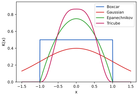
pp. 560–561 "Kernel" has several meanings in machine learning; here a density kernel is a function \(K:\R\to\R_+\) with \(\int K(x)\,\d x=1\) and \(K(-x)=K(x)\). Symmetry gives \(\int xK(x)\,\d x=0\) and hence \[ \int xK(x-x_n)\,\d x=x_n. \tag{16.25} \] Examples are the boxcar kernel \(K(x)=\frac12\ind(|x|\le1)\) (16.26) and the Gaussian kernel \(K(x)=(2\pi)^{-1/2}e^{-x^2/2}\) (16.27). The width is controlled by a bandwidth \(h\), \[ K_h(x)=\frac1hK\Big(\frac xh\Big), \tag{16.28} \] and for vector inputs one takes a radial basis function kernel \(K_h(\bm x)\propto K_h(\|\bm x\|)\) (16.29), which for the Gaussian is \[ K_h(\bm x)=\frac1{h^D(2\pi)^{D/2}}\prod_{d=1}^D\exp\Big(-\frac{x_d^2}{2h^2}\Big). \tag{16.30} \] Gaussian kernels have unbounded support; the kernels of Table 16.1 have compact support, which can be computationally faster:
| Name | \(K(x)\) | \(\sigma_K^2=\int x^2K\) | \(R(K)=\int K^2\) |
|---|---|---|---|
| Gaussian | \((2\pi)^{-1/2}e^{-x^2/2}\) | 1 | \(1/(2\sqrt\pi)=0.2821\) |
| Boxcar | \(\frac12\ind(|x|\le1)\) | \(1/3\) | \(1/2\) |
| Epanechnikov | \(\frac34(1-x^2)\ind(|x|\le1)\) | \(1/5\) | \(3/5\) |
| Tri-cube | \(\frac{70}{81}(1-|x|^3)^3\ind(|x|\le1)\) | \(35/243\) | \(175/247\) |
(Table 16.1 of the book; the last two columns are the moments used in Section 16.3.3 and are not in the book.) Figure 16.8 plots the four kernels.
Filling the gap 16.12: the normalising constants of Table 16.1, the moments of a density kernel, and what a KDE does to the mean and variance pp. 560–562, (16.25)–(16.33)
Derivation
Rescaling. \(\int K_h(x)\,\d x=\int\frac1hK(x/h)\,\d x=\int K(u)\,\d u=1\); \(\int xK_h(x)\,\d x=h\int uK(u)\,\d u=0\); \(\int x^2K_h(x)\,\d x=h^2\sigma_K^2\) with \(\sigma_K^2=\int u^2K(u)\,\d u\). (16.25) follows from the substitution \(u=x-x_n\): \(\int xK(x-x_n)\,\d x=\int(u+x_n)K(u)\,\d u=0+x_n\), and the same for \(K_h\).
Table 16.1. Boxcar: \(\frac12\cdot2=1\). Epanechnikov: \(\frac34\int_{-1}^1(1-x^2)\,\d x=\frac34(2-\frac23)=1\). Tri-cube: \(\int_{-1}^1(1-|x|^3)^3\,\d x=2\int_0^1(1-3x^3+3x^6-x^9)\,\d x=2(1-\frac34+\frac37-\frac1{10})=\frac{81}{70}\), so the constant is \(70/81\). Second moment of the tri-cube: \(\frac{140}{81}\int_0^1x^2(1-x^3)^3\,\d x=\frac{140}{81}\cdot\frac13\int_0^1(1-t)^3\,\d t=\frac{140}{243\cdot4}=\frac{35}{243}\) (substituting \(t=x^3\)). The others: boxcar \(\int_{-1}^1\frac{x^2}2\,\d x=\frac13\), Epanechnikov \(\frac34\int(x^2-x^4)=\frac34(\frac23-\frac25)=\frac15\). The roughness \(R(K)\) was evaluated by quadrature and agrees with the fractions in the table to \(10^{-8}\). (For a non-Gaussian radial kernel in (16.29) the proportionality constant is \(\big[\int K(\|\bm u\|)\,\d\bm u\big]^{-1}\); the Gaussian (16.30) is already normalised.)
The Parzen estimator \(\hat f(x)=\frac1N\sum_nK_h(x-x_n)\) (16.33). It is non-negative, and integrates to 1 because it is an average of densities. Its mean is \(\int x\hat f=\frac1N\sum_nx_n=\bar x\), by (16.25). Its variance is \(\frac1N\sum_n\int(x-\bar x)^2K_h(x-x_n)\,\d x=\frac1N\sum_n\big[(x_n-\bar x)^2+h^2\sigma_K^2\big]=s^2+h^2\sigma_K^2\), where \(s^2\) is the sample variance with divisor \(N\) (the cross term vanishes by symmetry). A KDE is therefore always wider than the sample by \(h^2\sigma_K^2\), a systematic oversmoothing (confirmed numerically for a Gaussian kernel). For the boxcar kernel, \(\hat f(x)=\frac1{2hN}\#\{n:|x-x_n|\le h\}\): the number of points within \(h\) divided by the width times \(N\).
16.3.2 Parzen window density estimator
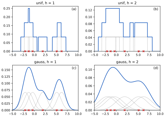
pp. 561–562 Recall the Gaussian mixture model of Section 3.5.1 with a fixed spherical covariance and uniform weights, \(p(\bm x\given\bm\theta)=\frac1K\sum_{k=1}^K\mathcal N(\bm x\given\bm\mu_k,\sigma^2\bm I)\) (16.31). It needs the number \(K\) of components and their locations. Allocating one component per data point removes both choices: \(p(\bm x\given\bm\theta)=\frac1N\sum_{n=1}^N\mathcal N(\bm x\given\bm x_n,\sigma^2\bm I)\) (16.32), and replacing the Gaussian by a general density kernel gives the Parzen window or kernel density estimator \[ p(\bm x\given\mathcal D)=\frac1N\sum_{n=1}^NK_h(\bm x-\bm x_n). \tag{16.33} \] No model fitting is needed beyond the choice of \(h\), and no number of clusters. The costs are memory (all data are stored) and evaluation time \(O(N)\) per point. Figure 16.9 shows the estimate from 6 points: the boxcar kernel gives a piecewise constant density that counts the points within \(h\), the Gaussian kernel a smooth density, and \(h\) controls the complexity.
See also: kernel density estimation with cross-validation (Nonparametric Statistical Inference) and choosing the bandwidth by cross-validation (Elements of Statistical Learning).
16.3.3 How to choose the bandwidth parameter
pp. 562–563 The bandwidth has a large effect (Figure 16.9) and can be viewed as controlling the complexity of the model. If the true density is Gaussian in one dimension, the bandwidth that is optimal for a Gaussian kernel, from the point of view of minimising the frequentist risk, is [BA97a] \[ h=\sigma\Big(\frac4{3N}\Big)^{1/5}, \] where \(\sigma\) can be estimated robustly by \(\hat\sigma=1.4826\,\mathrm{MAD}\), with \(\mathrm{MAD}=\operatorname{median}(|x-\operatorname{median}(x)|)\), the median absolute deviation. For \(D\) dimensions, estimate \(h_d\) in each coordinate and use their geometric mean \(h=(\prod_dh_d)^{1/D}\).
Filling the gap 16.13: bias, variance and AMISE of the KDE, the rule \(h=\sigma(4/3N)^{1/5}\), and the constant 1.4826 pp. 562–563, [BA97a]
Derivation
Bias. Let \(f\) be twice continuously differentiable with a bounded second derivative, and \(\hat f(x)=\frac1N\sum_nK_h(x-X_n)\) with \(K\) a symmetric density kernel with \(\sigma_K^2=\int u^2K<\infty\). Then \(\E\hat f(x)=\int K_h(x-y)f(y)\,\d y=\int K(u)f(x-hu)\,\d u\) and by Taylor's theorem \(f(x-hu)=f(x)-huf'(x)+\frac12h^2u^2f''(x)+o(h^2)\). The odd term integrates to 0, so \[ \operatorname{bias}\hat f(x)=\tfrac12h^2\sigma_K^2f''(x)+o(h^2). \] Variance. \(\hat f(x)\) is an average of i.i.d. variables \(Z_n=K_h(x-X_n)\), so \(\var\hat f(x)=\frac1N\var Z\le\frac1N\E Z^2\), and \(\E Z^2=\int K_h(x-y)^2f(y)\,\d y=\frac1h\int K(u)^2f(x-hu)\,\d u=\frac{f(x)R(K)}h(1+o(1))\) with \(R(K)=\int K^2\). Since \((\E Z)^2=O(1)\), \(\var\hat f(x)=\frac{f(x)R(K)}{Nh}+O(1/N)\).
AMISE. Integrating the squared bias and the variance over \(x\) (\(\int f=1\), \(R(f'')=\int f''^2\)), \[ \AMISE(h)=\frac{R(K)}{Nh}+\frac{h^4\sigma_K^4R(f'')}4. \] Setting the derivative to zero, \(-\frac{R(K)}{Nh^2}+h^3\sigma_K^4R(f'')=0\), gives \[ h^*=\Big(\frac{R(K)}{\sigma_K^4R(f'')N}\Big)^{1/5},\qquad\AMISE(h^*)=\tfrac54\big(\sigma_K^4R(K)^4R(f'')\big)^{1/5}N^{-4/5}. \] Gaussian reference. For \(f=\mathcal N(\mu,\sigma^2)\) and \(\phi\) the standard normal density, \(f''(x)=\sigma^{-3}(z^2-1)\phi(z)\) with \(z=(x-\mu)/\sigma\), so \(R(f'')=\sigma^{-5}\int(z^2-1)^2\phi^2\,\d z\). Since \(\phi^2(z)=\frac1{2\sqrt\pi}\,\mathcal N(z\given0,\tfrac12)\) and for \(Z\sim\mathcal N(0,\frac12)\), \(\E(Z^2-1)^2=\E Z^4-2\E Z^2+1=\frac34-1+1=\frac34\), \(R(f'')=\frac3{8\sqrt\pi\sigma^5}\). With the Gaussian kernel (\(\sigma_K=1\), \(R(K)=\frac1{2\sqrt\pi}\)), \[ h^*=\Big(\frac{1/(2\sqrt\pi)}{3/(8\sqrt\pi\sigma^5)\,N}\Big)^{1/5}=\Big(\frac{4\sigma^5}{3N}\Big)^{1/5}=\sigma\Big(\frac4{3N}\Big)^{1/5}\approx1.06\,\sigma N^{-1/5}, \] which is the rule of the book. It is the minimiser of the asymptotic risk; the minimiser of the exact MISE differs slightly (below).
The constant 1.4826. If \(X\sim\mathcal N(\mu,\sigma^2)\) then \(\operatorname{median}(X)=\mu\) and \(|X-\mu|/\sigma\) is half-normal with median \(\Phi^{-1}(3/4)=0.6745\); hence \(\operatorname{MAD}=0.6745\sigma\) and \(\sigma=\mathrm{MAD}/0.6745=1.4826\,\mathrm{MAD}\). Unlike the sample standard deviation the estimate is not inflated by outliers, and with data from \(\mathcal N(2,3^2)\) (\(2\times10^5\) draws) it returns 3.0.
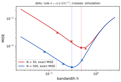
Exact MISE for Gaussian data. With \(f=\mathcal N(0,\sigma^2)\) and a Gaussian kernel, all integrals are Gaussian convolutions: \[ \MISE(h)=\frac1{2\sqrt\pi Nh}+\frac{1-1/N}{2\sqrt\pi\sqrt{\sigma^2+h^2}}-\frac{2}{\sqrt{2\pi}\sqrt{2\sigma^2+h^2}}+\frac1{2\sqrt\pi\sigma}. \] (The first term is \(R(K_h)/N\), the second \((1-1/N)\int(K_h*f)^2\), the third \(-2\int f(K_h*f)\), the fourth \(\int f^2\).) Quadrature of the bias-variance decomposition agreed with this formula, and simulation agreed with it as well. For \(\sigma=1\) the exact minimiser is \(h=0.52\) at \(N=50\) against the rule's \(0.48\), and \(0.313\) against \(0.306\) at \(N=500\) (Figure 16.S9).
Caveat. The rule is optimal for a Gaussian \(f\). For multimodal densities \(R(f'')\) is larger than the Gaussian value, so the optimal \(h^*\) is smaller and the rule oversmooths (demonstration, preset 3).
16.3.4 From KDE to KNN classification
p. 563 KNN was introduced as a heuristic, but it is also a generative classifier whose class-conditional densities are modelled by a KDE with a variable bandwidth. Instead of a fixed bandwidth and counting the points within a fixed hypercube, "grow" a volume around \(\bm x\) until it contains \(K\) points regardless of class: a balloon kernel density estimator [TS92]. Let \(V(\bm x)\) be the volume and \(N_c(\bm x)\) the number of the \(K\) points of class \(c\) in it, and \(N_c\) the number of class-\(c\) points in the whole data set. Then \[ p(\bm x\given y=c,\mathcal D)=\frac{N_c(\bm x)}{N_cV(\bm x)}, \tag{16.34} \] and with the class prior \(p(y=c)=N_c/N\), \[ p(y=c\given\bm x,\mathcal D)=\frac{\frac{N_c(\bm x)}{N_cV(\bm x)}\frac{N_c}N}{\sum_{c'}\frac{N_{c'}(\bm x)}{N_{c'}V(\bm x)}\frac{N_{c'}}N}=\frac{N_c(\bm x)}{\sum_{c'}N_{c'}(\bm x)}=\frac{N_c(\bm x)}K=\frac1K\sum_{n\in\mathcal N_K(\bm x,\mathcal D)}\ind(y_n=c), \tag{16.35} \] using \(\sum_cN_c(\bm x)=K\): this is (16.1).
Filling the gap 16.14: the algebra of (16.35), and why (16.34) is not a density p. 563, (16.34), (16.35)
Derivation
Algebra. In (16.35) the factor \(N_c\) in the denominator of (16.34) cancels the prior \(N_c/N\), so the numerator is \(N_c(\bm x)/(NV(\bm x))\); the denominator is the sum of the same expression over \(c'\), \(\sum_{c'}N_{c'}(\bm x)/(NV(\bm x))\), and the common factor \(1/(NV(\bm x))\) cancels. The result \(N_c(\bm x)/K\) does not depend on how \(V\) is defined, only that the same ball is used for every class. A numerical experiment with 60 random planar points and \(K=7\) gave the vote shares exactly.
What the book's wording hides. The book says the bandwidth "is allowed to be different for each data point". In the balloon estimator the volume depends on the query \(\bm x\) (it is grown around the point where the density is evaluated), not on the sample points; the estimator that varies the bandwidth with the sample points is the sample-point estimator.
(16.34) is not a probability density. In one dimension \(V(x)=2r_K(x)\) with \(r_K(x)\) the distance to the \(K\)-th nearest point, and for large \(|x|\), \(r_K(x)\sim|x|\). Then \(\hat p(x)=K/(NV(x))\) behaves like \(K/(2N|x|)\) in both tails and \(\int\hat p(x)\,\d x\) diverges logarithmically (numerically, the mass within \([-R,R]\) of the \(K=3\) estimate for 50 Gaussian points is 1.64, 1.78, 1.92 for \(R=20,200,2000\): it keeps growing by about 0.14 per decade of \(R\)). The posterior (16.35) is nevertheless a proper distribution, because the divergent normaliser cancels between numerator and denominator. So the KNN classifier is a generative classifier in the sense of Bayes' rule applied to unnormalised class-conditional estimates.
16.3.5 Kernel regression
pp. 563–565 As KDE underlies a generative classifier, it also underlies a generative regression model.
16.3.5.1 Nadaraya-Watson estimator for the mean
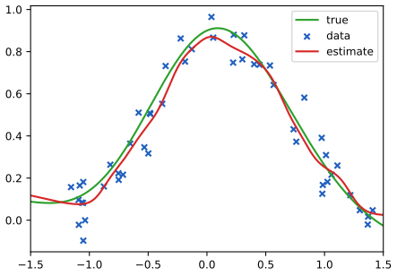
The goal is \(\E[y\given\bm x,\mathcal D]=\int y\,p(y\given\bm x,\mathcal D)\,\d y=\frac{\int y\,p(\bm x,y\given\mathcal D)\,\d y}{\int p(\bm x,y\given\mathcal D)\,\d y}\) (16.36). If \(p(\bm x,y)\) is modelled as a multivariate normal, the result is linear regression (Section 11.2.3.5), too restrictive in general. A KDE approximates the joint density without that assumption: \[ p(y,\bm x\given\mathcal D)\approx\frac1N\sum_{n=1}^NK_h(\bm x-\bm x_n)K_h(y-y_n). \tag{16.37} \] Using (16.25) for \(\int yK_h(y-y_n)\,\d y=y_n\) and \(\int K_h(y-y_n)\,\d y=1\), \[ \E[y\given\bm x,\mathcal D]=\frac{\sum_{n=1}^NK_h(\bm x-\bm x_n)\,y_n}{\sum_{n'=1}^NK_h(\bm x-\bm x_{n'})}=\sum_{n=1}^Ny_nw_n(\bm x),\qquad w_n(\bm x)=\frac{K_h(\bm x-\bm x_n)}{\sum_{n'}K_h(\bm x-\bm x_{n'})}, \tag{16.38, 16.39, 16.40} \] a weighted average of the training responses, with weights that depend on the similarity of \(\bm x\) to the stored inputs. This is kernel regression, kernel smoothing or the Nadaraya-Watson (N-W) estimator. Section 17.2.3 relates it to Gaussian process regression. Figure 16.10 shows a fit in one dimension with a Gaussian kernel.
16.3.5.2 Estimator for the variance
The predictive variance follows from \(\var[y\given\bm x,\mathcal D]=\E[y^2\given\bm x,\mathcal D]-\mu(\bm x)^2\) (16.41) with \(\mu(\bm x)\) the N-W mean. For a Gaussian kernel of variance \(\sigma^2\) in \(y\), \[ \E[y^2\given\bm x,\mathcal D]=\frac{\sum_nK_h(\bm x-\bm x_n)(\sigma^2+y_n^2)}{\sum_{n'}K_h(\bm x-\bm x_{n'})} \tag{16.42, 16.43} \] using \(\int y^2\mathcal N(y\given y_n,\sigma^2)\,\d y=\sigma^2+y_n^2\) (16.44), so that \[ \var[y\given\bm x,\mathcal D]=\sigma^2+\sum_{n=1}^Nw_n(\bm x)y_n^2-\mu(\bm x)^2. \tag{16.45} \] This matches the estimator of [BA10] up to the initial \(\sigma^2\) term.
16.3.5.3 Locally weighted regression
Dropping the normalisation of (16.39) gives \(\mu(\bm x)=\sum_ny_nK_h(\bm x-\bm x_n)\) (16.46). Rather than only interpolating the stored responses one can fit a locally linear model around each query, \[ \mu(\bm x)=\min_{\bm\beta}\sum_{n=1}^N\big[y_n-\bm\beta^\T\bm\phi(\bm x_n)\big]^2K_h(\bm x-\bm x_n),\qquad\bm\phi(\bm x)=[1,\bm x], \tag{16.47} \] called locally linear regression or LOWESS/LOESS [CD88], often used to annotate scatter plots with a local trend line.
Filling the gap 16.15: the derivation of the Nadaraya-Watson mean and variance, its limits, and the meaning of (16.45) pp. 563–565, (16.36)–(16.45)
Derivation
(16.39). Substituting (16.37) in (16.36), the numerator is \(\frac1N\sum_nK_h(\bm x-\bm x_n)\int yK_h(y-y_n)\,\d y=\frac1N\sum_nK_h(\bm x-\bm x_n)y_n\) and the denominator is \(\frac1N\sum_nK_h(\bm x-\bm x_n)\int K_h(y-y_n)\,\d y=\frac1N\sum_nK_h(\bm x-\bm x_n)\); the factors \(1/N\) cancel. The numerical experiment: with a Gaussian \(K_h\) of bandwidth 0.2 in \(x\) and 0.15 in \(y\), the ratio of integrals of the product-kernel KDE of 60 simulated points equals the sum \(\sum y_nw_n(x)\) to \(10^{-6}\) (quadrature over \(y\)). Note that the bandwidth of the kernel in \(y\) is irrelevant to the mean.
Properties. The weights are non-negative and sum to one, so \(\mu(\bm x)\) is a convex combination of the responses and lies in \([\min y_n,\max y_n]\). It minimises the local weighted squared error: \(\frac{\partial}{\partial a}\sum_nw_n(\bm x)(y_n-a)^2=-2\sum_nw_n(y_n-a)=0\iff a=\sum_nw_ny_n\). Limits for the Gaussian kernel: as \(h\to\infty\) all weights tend to \(1/N\) and \(\mu\) tends to the sample mean \(\bar y\); as \(h\to0\) the weight concentrates on the nearest input (\(w_n\propto e^{-\|\bm x-\bm x_n\|^2/2h^2}\), and the ratio of exponentials of two distances goes to 0 or \(\infty\)), so \(\mu\) tends to the 1-NN prediction (a piecewise constant function on the Voronoi cells). The boxcar kernel with a data-driven bandwidth giving exactly \(K\) points is KNN regression.
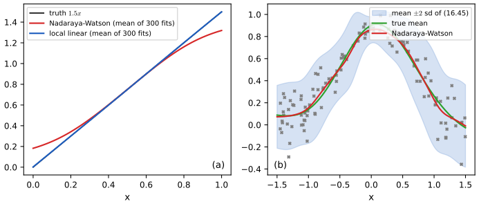
(16.45). \(\E[y^2\given\bm x]=\sum_nw_n(\bm x)\int y^2\mathcal N(y\given y_n,\sigma^2)\,\d y=\sum_nw_n(\sigma^2+y_n^2)\), since the second moment is the variance plus the squared mean. Subtracting \(\mu^2\) and using \(\sum_nw_n=1\), \[ \var[y\given\bm x]=\sigma^2+\sum_nw_n(\bm x)\,(y_n-\mu(\bm x))^2\ \ge\ \sigma^2. \] So (16.45) is the kernel variance plus the weighted sample variance of the nearby responses. That includes both the noise of the data and the variation of the regression function across the window: where the true curve is steep and the bandwidth is not small, the estimate overstates the noise level (Figure 16.S8b). It is not the variance of the estimator \(\mu(\bm x)\) (which is smaller by a factor of the effective number of points in the window), but of the predictive distribution of a new \(y\). (A quadrature check of the variance of the same product-kernel density agreed to \(10^{-6}\).)
Filling the gap 16.16: the unnormalised sum (16.46), locally linear regression (16.47), exactness for linear functions, and the boundary bias of Nadaraya-Watson p. 565, (16.46), (16.47), [CD88]
Derivation
(16.46) is not an estimate of the mean. The unnormalised sum is \(\sum_ny_nK_h(\bm x-\bm x_n)=\big[\sum_nK_h(\bm x-\bm x_n)\big]\mu_{\rm NW}(\bm x)=N\hat f_{\bm X}(\bm x)\,\mu_{\rm NW}(\bm x)\), with \(\hat f_{\bm X}\) the KDE of the inputs, so it estimates \(N f_{\bm X}(\bm x)\,m(\bm x)\) (the regression function times the design density times \(N\)), not \(m(\bm x)\). It is the numerator of (16.39) and needs the denominator.
(16.47) in detail. The minimum is over \(\bm\beta\), and the prediction is the fitted line evaluated at the query: \(\hat{\bm\beta}(\bm x)=\arg\min_{\bm\beta}\sum_nK_h(\bm x-\bm x_n)(y_n-\beta_0-\beta_1(\bm x_n-\bm x))^2\) and \(\mu(\bm x)=\hat\beta_0(\bm x)\). Centring the feature at the query makes the intercept the prediction. With \(\bm B\) the matrix with rows \([1,x_n-x]\) and \(\bm W=\diag(K_h(x-x_n))\), \(\hat{\bm\beta}=(\bm B^\T\bm W\bm B)^{-1}\bm B^\T\bm W\bm y\), so \(\mu(x)=\sum_n\ell_n(x)y_n\) with the equivalent kernel \(\ell_n(x)=\bm e_1^\T(\bm B^\T\bm W\bm B)^{-1}\bm B^\T\bm W\bm e_n\); this is a linear smoother like N-W.
Exactness for linear functions. If \(y_n=a+bx_n\) then \(y_n=a+b x+b(x_n-x)\) lies in the column space of \(\bm B\), so the weighted least-squares fit is exact with \(\hat\beta_0=a+bx=m(x)\). Equivalently, \(\sum_n\ell_n=1\) and \(\sum_n\ell_n(x_n-x)=0\). (A numerical test with \(y=2-3x\) at \(x=0,0.5,1\), including the boundary, returned the exact values.) The N-W estimator has only the first property.
Boundary bias of N-W. Take \(m(x)=a+bx\) with the design uniform on \([0,\infty)\) and evaluate at the boundary \(x=0\): in the limit of many points, \(\mu_{\rm NW}(0)=\frac{\int_0^\infty(a+bu)K_h(u)\,\d u}{\int_0^\infty K_h(u)\,\d u}=a+bh\,\frac{\int_0^\infty vK(v)\,\d v}{\int_0^\infty K(v)\,\d v}=a+2bh\int_0^\infty vK(v)\,\d v\), because \(\int_0^\infty K=\frac12\). For the Gaussian kernel \(2\int_0^\infty vK(v)\,\d v=\sqrt{2/\pi}\), so the bias is \(bh\sqrt{2/\pi}\), of order \(h\) (not \(h^2\)): with \(b=1.5\), \(h=0.15\) it is 0.1795, matching a simulation with 20 000 points (0.1795) and the average of 300 fits of 100 points (0.18, Figure 16.S8a). Local linear regression has no such bias for linear \(m\), and for general smooth \(m\) its bias at the boundary is \(O(h^2)\).
Interior bias. For an interior point and a symmetric kernel, Taylor expansion of numerator \(\int m(x-hu)f_X(x-hu)K(u)\,\d u\) and denominator \(\int f_X(x-hu)K(u)\,\d u\) to second order gives \(\E\mu_{\rm NW}(x)\approx m+\frac{h^2\sigma_K^2}2\big[m''+2m'f_X'/f_X\big]\), because \((mf_X)''-mf_X''=m''f_X+2m'f_X'\). The second term (the design bias) depends on the density of the inputs; local linear regression has only \(\frac{h^2\sigma_K^2}2m''\). A uniform design (\(f_X'=0\)) with \(m=x^2\), \(h=0.1\) gives a bias \(h^2=0.0100\) at 0 (simulated: 0.0102).
LOWESS. The classical LOWESS/LOESS of Cleveland and Devlin [CD88] uses the tri-cube kernel with a bandwidth set by a fixed fraction of the nearest data points (a nearest-neighbour span) and optional robustness iterations that down-weight large residuals; (16.47) is the basic non-robust fit.
See also: local regression at the boundary (Elements of Statistical Learning), regressograms and kernel local averages and kernel functions and Nadaraya-Watson regression (Bayesian and Probabilistic Machine Learning).
Exercises
The book has no end-of-chapter exercises for Chapter 16 (the chapter ends at page 565 with Section 16.3.5.3). The six exercises below are my own, written to cover the computations and proofs the chapter invites; each has a complete solution (hidden). Numerical answers were obtained with the code of this chapter.
Exercise 16.1 (KNN by hand). The one-dimensional training set is \(x=(1,2,4,7,8.5,9.8,12)\) with labels \(y=(0,0,1,1,0,1,1)\). (a) Compute \(p(y=1\given x=6,\mathcal D)\) from (16.1) for \(K=1,3,5\). (b) Compute the leave-one-out error (each point excluded from its own neighbourhood) of the 1-NN and the 3-NN classifier. (c) Why is the training error of 1-NN equal to 0 here, and what is its leave-one-out error doing?
Solution
(a) Distances from 6: \(7\) (1.0, label 1), \(4\) (2.0, label 1), \(8.5\) (2.5, label 0), \(9.8\) (3.8, label 1), \(2\) (4.0, label 0), \(1\) (5.0, label 0), \(12\) (6.0, label 1). For \(K=1\): \(\{7\}\), labels \(\{1\}\), \(p=1\). For \(K=3\): \(\{7,4,8.5\}\), labels \((1,1,0)\), \(p=2/3\). For \(K=5\): add \(9.8\) and \(2\): labels \((1,1,0,1,0)\), \(p=3/5\).
(b) 1-NN: the nearest other point of \(1\) is \(2\) (label 0, correct); of \(2\) is \(1\) (0, correct); of \(4\) is \(2\) (0, wrong, \(y=1\)); of \(7\) is \(8.5\) (0, wrong); of \(8.5\) is \(9.8\) (1, wrong, \(y=0\)); of \(9.8\) is \(8.5\) (0, wrong); of \(12\) is \(9.8\) (1, correct). Four errors of seven: \(4/7=0.571\). 3-NN: \(x=1\): neighbours \(2,4,7\), labels \((0,1,1)\), predicts 1, wrong; \(x=2\): \((0,1,1)\), wrong; \(x=4\): neighbours \(2,1,7\), labels \((0,0,1)\), predicts 0, wrong; \(x=7\): \(8.5,9.8,4\), \((0,1,1)\), predicts 1, correct; \(x=8.5\): \(9.8,7,12\), \((1,1,1)\), wrong; \(x=9.8\): \(8.5,12,7\), \((0,1,1)\), correct; \(x=12\): \(9.8,8.5,7\), \((1,0,1)\), correct. Four errors: \(4/7=0.571\) again. (Confirmed with the code.)
(c) Each training point is its own nearest neighbour at distance 0 and, with distinct inputs, the only point at distance 0, so the 1-NN rule returns its own label: training error 0. The leave-one-out error removes that self-vote and measures the real predictive ability, here 4/7, worse than the 3/7 that guessing the majority label (class 1, four of seven) would give. The two numbers are far apart: the training error is useless for choosing \(K\) (Figure 16.2d). \(\square\)
Exercise 16.2 (Voronoi cells). (a) Show that the set of points whose nearest training input is \(\bm x_n\) is a convex polytope. (b) Show that the training error of 1-NN is 0 if and only if no two identical inputs carry different labels (with ties broken arbitrarily). (c) Give a data set in which the 1-NN training error is 0 but its leave-one-out error is 1.
Solution
(a) \(V(\bm x_n)=\bigcap_{m\ne n}\{\bm x:\|\bm x-\bm x_n\|^2\le\|\bm x-\bm x_m\|^2\}\), and \(\|\bm x-\bm x_n\|^2\le\|\bm x-\bm x_m\|^2\iff2(\bm x_m-\bm x_n)^\T\bm x\le\|\bm x_m\|^2-\|\bm x_n\|^2\) is a half-space (a half-line in 1-D). An intersection of finitely many half-spaces is a convex polytope (possibly unbounded).
(b) If the inputs are distinct, \(\bm x_n\) is the unique point at distance 0 from itself, so the prediction at \(\bm x_n\) is \(y_n\): no training error. If \(\bm x_i=\bm x_j\) with \(y_i\ne y_j\), then at this input both points are at distance 0, the rule returns one of the two labels (whatever the tie rule), and exactly one of the two training points is misclassified: the training error is positive. If identical inputs always share their label, ties among them do not matter and the error is 0.
(c) Take \(x_n=n\), \(n=1,\dots,N\), with alternating labels \(0,1,0,1,\dots\). For an interior point both neighbours at distance 1 have the opposite label, so the leave-one-out 1-NN prediction is wrong; the end points have a single neighbour, also of the opposite label. The leave-one-out error is 1 while the training error is 0. \(\square\)
Exercise 16.3 (margins on the sphere, and the N-pairs gradient). (a) For unit-norm embeddings show that the triplet loss (16.11) with margin \(m\) equals \(2\,[\hat{\bm e}_a^\T\hat{\bm e}_n-\hat{\bm e}_a^\T\hat{\bm e}_p+m/2]_+\), so that it is the hinge loss (16.15) with margin 1 when \(m=2\). (b) Let \(\hat{\bm e}_a=(1,0,0)\), \(\hat{\bm e}_p=(1,1,0)/\sqrt2\) and the negatives \((0,1,0)\), \((0,0,1)\), \((-1,1,0)/\sqrt2\). With temperature \(\tau=1\), compute the softmax probabilities of the positive and the negatives and the gradient of the N-pairs loss with respect to \(\hat{\bm e}_a\).
Solution
(a) By (16.9), \(d_{ap}^2-d_{an}^2=(2-2s_p)-(2-2s_n)=2(s_n-s_p)\) with \(s_p=\hat{\bm e}_a^\T\hat{\bm e}_p\), \(s_n=\hat{\bm e}_a^\T\hat{\bm e}_n\). Hence \([d_{ap}^2-d_{an}^2+m]_+=[2(s_n-s_p)+m]_+=2[s_n-s_p+m/2]_+\). For \(m=2\) this is twice the hinge (16.15), \([s_n-s_p+1]_+\), so squared-distance triplet training with margin \(m\) on the sphere is a cosine-similarity hinge with margin \(m/2\).
(b) The similarities are \(s_+=1/\sqrt2=0.7071\) and \(s=(0,0,-0.7071)\), so the unnormalised weights are \(e^{0.7071}=2.028\), \(1\), \(1\), \(e^{-0.7071}=0.493\), with sum 4.521; the probabilities are \(\pi_+=0.4486\) and \(\pi=(0.2212,0.2212,0.1091)\). By gap 16.8(d), \(\partial L/\partial\hat{\bm e}_a=\sum_k\pi_k\hat{\bm e}_k-(1-\pi_+)\hat{\bm e}_+\). The first sum is \(0.2212(0,1,0)+0.2212(0,0,1)+0.1091(-1,1,0)/\sqrt2=(-0.0771,0.2983,0.2212)\) and \((1-\pi_+)\hat{\bm e}_+=0.5514\cdot(0.7071,0.7071,0)=(0.3899,0.3899,0)\); the gradient is \((-0.4670,-0.0916,0.2212)\). A finite-difference check reproduced it. Descent moves \(\hat{\bm e}_a\) in the direction \((0.467,0.092,-0.221)\): the first two coordinates move towards the positive, and the third decreases because the negative \((0,0,1)\) carries probability 0.2212; the negative \((-1,1,0)/\sqrt2\) has the smallest weight (0.1091) because it is the least similar to the anchor. \(\square\)
Exercise 16.4 (which kernel is best?). Use the AMISE of gap 16.13. (a) Show that at the optimal bandwidth the AMISE is proportional to \((\sigma_KR(K))^{4/5}N^{-4/5}\) and that two kernels reach the same AMISE with sample sizes in the ratio \(N_E/N_K=\sigma_ER(E)/(\sigma_KR(K))\); compute this efficiency for the four kernels of Table 16.1 relative to the Epanechnikov kernel. (b) For Gaussian data, give the optimal bandwidth of the Epanechnikov kernel.
Solution
(a) From gap 16.13, \(\AMISE(h^*)=\frac54(\sigma_K^4R(K)^4R(f''))^{1/5}N^{-4/5}=\frac54(\sigma_KR(K))^{4/5}R(f'')^{1/5}N^{-4/5}\). Equating this for kernels \(E\) and \(K\) gives \(N_E^{-4/5}(\sigma_ER_E)^{4/5}=N_K^{-4/5}(\sigma_KR_K)^{4/5}\), that is \(N_E/N_K=\sigma_ER_E/(\sigma_KR_K)\), independent of \(f\). The products \(\sigma_KR(K)\): Gaussian \(0.2821\), boxcar \(0.2887\), Epanechnikov \(\frac1{\sqrt5}\cdot\frac35=0.2683\), tri-cube \(\sqrt{35/243}\cdot\frac{175}{247}=0.2689\). Efficiencies relative to the Epanechnikov kernel: boxcar \(0.930\), Gaussian \(0.951\), tri-cube \(0.998\), Epanechnikov 1. The choice of kernel matters little (a Gaussian kernel needs about 5% more data than the Epanechnikov kernel for the same AMISE); the bandwidth matters far more.
(b) \(h^*=\big(R(E)/(\sigma_E^4R(f'')N)\big)^{1/5}\) with \(R(E)=\frac35\), \(\sigma_E^4=\frac1{25}\), \(R(f'')=\frac3{8\sqrt\pi\sigma^5}\): \(h^*=\big(\frac{3/5}{(1/25)\cdot3/(8\sqrt\pi\sigma^5)\,N}\big)^{1/5}=\sigma\big(\frac{40\sqrt\pi}N\big)^{1/5}=2.34\,\sigma N^{-1/5}\), about 2.2 times the Gaussian-kernel bandwidth \(1.06\,\sigma N^{-1/5}\). This is consistent with the kernels' widths: the Epanechnikov kernel has standard deviation \(\sigma_E=0.447\) so its effective width \(h\sigma_E\approx1.05\,\sigma N^{-1/5}\) is the same as the Gaussian's. \(\square\)
Exercise 16.5 (boundary bias). Let \(m(x)=a+bx\), the design uniform on \([0,\infty)\), and let \(K_h\) be a symmetric kernel. (a) Find the limiting bias of the Nadaraya-Watson estimator at \(x=0\) for the Gaussian, boxcar and Epanechnikov kernels. (b) Show that local linear regression has zero bias there. (c) Evaluate (a) for \(b=1.5\) and \(h=0.15\).
Solution
(a) From gap 16.16, the bias is \(bh\,\beta_K\) with \(\beta_K=\int_0^\infty vK(v)\,\d v\big/\int_0^\infty K(v)\,\d v=2\int_0^\infty vK(v)\,\d v\). Gaussian: \(2\cdot\frac1{\sqrt{2\pi}}=\sqrt{2/\pi}=0.7979\). Boxcar: \(2\int_0^1\frac v2\,\d v=\frac12\). Epanechnikov: \(2\cdot\frac34\int_0^1v(1-v^2)\,\d v=\frac32\cdot\frac14=\frac38\). So the bias is \(0.798bh\), \(0.5bh\) and \(0.375bh\).
(b) The data lie exactly on a line, and the weighted least-squares line fitted at \(x=0\) is the same line (gap 16.16, exactness for linear functions), so \(\hat\beta_0=a\) for every \(h\) and every kernel.
(c) \(0.7979\times1.5\times0.15=0.1795\) for the Gaussian kernel (simulation with 20 000 points: 0.1795), \(0.1125\) for the boxcar and \(0.084\) for the Epanechnikov kernel. The bias is first order in \(h\), whereas interior bias is second order. \(\square\)
Exercise 16.6 (latent coincidence analysis). Take \(L=1\), \(\kappa=1\), \(\sigma^2=\frac12\) and a pair with \(m=W(x-x')=1\). (a) Compute \(p(y=1\given x,x')\), and the posterior mean and variance of \(u=z-z'\) given \(y=1\). (b) Show that \(p(y=1\given x,x')\) is unchanged when \((W,\sigma^2,\kappa^2)\) is replaced by \((cW,c^2\sigma^2,c^2\kappa^2)\). (c) What is the largest value \(p(y=1\given x,x')\) can take for given \(\sigma^2\) and \(L\)? What does it say about the model?
Solution
(a) By gap 16.7, \(A=(1+2\sigma^2/\kappa^2)^{-L/2}\exp\big(-m^2/(2(\kappa^2+2\sigma^2))\big)=2^{-1/2}e^{-1/4}=0.5507\). The posterior of \(u\) given \(y=1\) is Gaussian with variance \(s^2=(\frac1{2\sigma^2}+\frac1{\kappa^2})^{-1}=(1+1)^{-1}=\frac12\) and mean \(m_1=\frac{s^2}{2\sigma^2}m=\frac{1/2}{1}\cdot1=\frac12\). (Prior mean 1 shrunk towards 0 by the coincidence factor \(e^{-u^2/2}\).)
(b) The exponent is \(\|cW d\|^2/(2(c^2\kappa^2+2c^2\sigma^2))=\|Wd\|^2/(2(\kappa^2+2\sigma^2))\) and \(1+2c^2\sigma^2/(c^2\kappa^2)=1+2\sigma^2/\kappa^2\): both unchanged. This is why \(\kappa=1\) is without loss of generality.
(c) For identical inputs \(m=0\) and \(A=(1+2\sigma^2/\kappa^2)^{-L/2}<1\); this is the supremum. LCA never assigns probability 1 to a match unless \(\sigma^2\to0\): the latent noise caps how confident a "same" decision can be, which is a property of the likelihood to remember when interpreting \(p(y=1\given x,x')\) as a calibrated probability. For \(\sigma^2=\frac12\), \(L=1\): \(\sup A=0.7071\). \(\square\)
Demonstrations
| Page | What it shows | In the notes |
|---|---|---|
| K nearest neighbour regions and the choice of K | A three-class problem in the plane: majority-vote regions, the vote at a clicked point, the train and test error against \(K\), and a Mahalanobis stretch of one axis. Presets: 1 K = 1, Voronoi cells; 2 the vote at a point; 3 K = 15; 4 K = 80; 5 stretched axis. | 16.1.1, gap 16.1 |
| The curse of dimensionality for nearest neighbours | Uniform data in the cube with two informative coordinates and many noise ones: test error against the dimension, the edge length \((K/N)^{1/D}\), and a metric that ignores the noise. Presets: 1 two coordinates; 2 eight noise coordinates; 3 twenty-eight; 4 fewer points; 5 larger K. | 16.1.2, gap 16.2 |
| Learning a metric: neighbourhood components analysis | Gradient ascent on the NCA objective for a tilted two-class problem with a large nuisance direction, the data before and after the learned map, and the leave-one-out error; a second data set where there is nothing to learn. Presets: 1 Euclidean start; 2 100 steps; 3 1000 steps; 4 four blobs; 5 neighbours of a point. | 16.2.1.2, gap 16.6 |
| Kernel density estimation and kernel regression | Parzen estimates with four kernels and a chosen bandwidth, the rule-of-thumb bandwidth, and Nadaraya-Watson against local linear regression with the spread band of (16.45). Presets: 1 six points, boxcar; 2 six points, Gaussian; 3 bimodal sample at the rule bandwidth; 4 Nadaraya-Watson with the band; 5 boundary bias. | 16.3.2, 16.3.3, 16.3.5, gaps 16.13, 16.15, 16.16 |
The Python code that produces every figure of this page is code/ch16_exemplar_based_methods.py (see the code index). Companion demos: the bias-variance trade-off for k-nearest-neighbour regression, the Cover-Hart bound, histograms, kernel density estimates and nearest neighbours, local polynomial regression with cross-validation.
Notes on the book
Points where the book is imprecise or wrong
- Section 16.2.5.3, the sign of the gap. The book states \(0\le L_t-L_u\le\frac{N^3}{C^2}K\). Its own (16.21) says \(L_t\le L_u\), so the difference \(L_t-L_u\) is non-positive; the statement should read \(0\le L_u-L_t\). I confirmed numerically that \(L_t\le L_u\) for random embeddings, and derived the sharper bound \(L_u-L_t\le4a\sum_i\delta_i\) (gap 16.10).
- (16.22), inputs for embeddings. The right-hand side writes \(\|\bm x_i-\bm c_{y_i}\|\) and \(\|\bm x_i-\bm c_m\|\), with the input \(\bm x_i\); the bound is in terms of the embedding \(\hat{\bm e}_i\), as in (16.20) (gap 16.10). The closed form, including the constant \(C'\), is correct.
- (16.47), min against argmin. The formula writes \(\mu(\bm x)=\min_{\bm\beta}\sum_n[\ldots]\), which is the minimum value of the weighted loss, not a prediction. The prediction is \(\hat{\bm\beta}(\bm x)^\T\bm\phi(\bm x)\) with \(\hat{\bm\beta}\) the minimiser, or, with the feature centred at the query, the intercept \(\hat\beta_0(\bm x)\) (gap 16.16).
- Section 16.2.1.3, the coincidence kernel. The text gives \(p(y=1\given\bm z,\bm z')=\exp(-\frac1{2\kappa^2}\|\bm z-\bm z'\|)\) without the square. The closed-form marginal and the closed-form E step hold only for the squared norm, \(\exp(-\frac1{2\kappa^2}\|\bm z-\bm z'\|^2)\), which is what the notes use (gap 16.7). Also the statement that EM "does not need step size adjustment" is true, but EM can be slow when the supremum is approached at the boundary \(\sigma^2\to0\), as on the toy data of Figure 16.S5.
- Section 16.1, "within a factor of 2 of the Bayes error". The statement is for the 1-NN rule and the limit \(N\to\infty\) in a fixed dimension; the precise bound is \(R^*(2-\frac C{C-1}R^*)\), which is \(2R^*(1-R^*)\) for two classes (gap 16.1). For larger fixed \(K\) the limit is smaller, and the rule is consistent when \(K\to\infty\) with \(K/N\to0\).
- (16.11) against (16.16). The triplet loss is defined on squared distances but the hard/semi-hard/easy taxonomy on plain distances. The two margins differ (squared: \(d_n^2\ge d_p^2+m\); plain: \(d_n\ge d_p+m\)), so a "semi-hard" negative of (16.16) can have zero squared-distance loss (gap 16.9).
- Section 16.3.3, "optimal bandwidth". \(h=\sigma(4/3N)^{1/5}\) minimises the asymptotic mean integrated squared error for Gaussian data and a Gaussian kernel; the minimiser of the exact MISE is a few percent larger (7 percent at \(N=50\)) (gap 16.13). It also oversmooths multimodal densities.
- Section 16.3.4, "different for each data point". The volume in (16.34) is grown around the query \(\bm x\); it varies with the query, not with the training points. And \(p(\bm x\given y=c,\mathcal D)=N_c(\bm x)/(N_cV(\bm x))\) is not normalised (in one dimension its integral diverges), which is harmless because the posterior (16.35) only needs ratios (gap 16.14).
- Section 16.1.3, "intractable above about 10 dimensions". Exact search by space partitioning degrades to a linear scan; "intractable" here is empirical (a k-d tree needs about \(2^D\) cells visited, Figure 16.S3a), not a complexity-theoretic statement (gap 16.3).
- (16.46), the unnormalised sum. Dropping the denominator of (16.39) gives \(N\hat f_{\bm X}(\bm x)\mu_{\rm NW}(\bm x)\), which estimates the regression function multiplied by the input density (times \(N\)), not the regression function (gap 16.16).
References
- Murphy, K. P. (2022). Probabilistic Machine Learning: An Introduction. MIT Press, Cambridge, MA. Chapter 16, pp. 547–565. probml.github.io/pml-book/book1.html.
- Bowman, A. W. and Azzalini, A. (1997). Applied Smoothing Techniques for Data Analysis. Oxford University Press.
- Chaudhuri, K. and Dasgupta, S. (2014). Rates of convergence for nearest neighbor classification. Advances in Neural Information Processing Systems, 27.
- Chen, T., Kornblith, S., Norouzi, M. and Hinton, G. (2020). A simple framework for contrastive learning of visual representations. International Conference on Machine Learning.
- Chopra, S., Hadsell, R. and LeCun, Y. (2005). Learning a similarity metric discriminatively, with application to face verification. IEEE Conference on Computer Vision and Pattern Recognition.
- Cleveland, W. S. and Devlin, S. J. (1988). Locally weighted regression: an approach to regression analysis by local fitting. Journal of the American Statistical Association, 83(403), 596–610.
- Cover, T. M. and Hart, P. E. (1967). Nearest neighbor pattern classification. IEEE Transactions on Information Theory, 13(1), 21–27.
- Der, R. and Saul, L. (2012). Latent coincidence analysis: a hidden variable model for distance metric learning. Advances in Neural Information Processing Systems, 25.
- Do, T.-T., Tran, T., Reid, I., Kumar, V., Hoang, T. and Carneiro, G. (2019). A theoretically sound upper bound on the triplet loss for improving the efficiency of deep distance metric learning. IEEE Conference on Computer Vision and Pattern Recognition.
- Epanechnikov, V. A. (1969). Non-parametric estimation of a multivariate probability density. Theory of Probability and its Applications, 14(1), 153–158.
- Gionis, A., Indyk, P. and Motwani, R. (1999). Similarity search in high dimensions via hashing. Proceedings of the 25th International Conference on Very Large Data Bases.
- Goldberger, J., Roweis, S., Hinton, G. and Salakhutdinov, R. (2005). Neighbourhood components analysis. Advances in Neural Information Processing Systems, 17.
- Johnson, J., Douze, M. and Jégou, H. (2019). Billion-scale similarity search with GPUs. IEEE Transactions on Big Data, 7(3), 535–547.
- Marsaglia, G. (1972). Choosing a point from the surface of a sphere. Annals of Mathematical Statistics, 43(2), 645–646.
- Movshovitz-Attias, Y., Toshev, A., Leung, T. K., Ioffe, S. and Singh, S. (2017). No fuss distance metric learning using proxies. IEEE International Conference on Computer Vision.
- Musgrave, K., Belongie, S. and Lim, S.-N. (2020). A metric learning reality check. European Conference on Computer Vision.
- Nadaraya, E. A. (1964). On estimating regression. Theory of Probability and its Applications, 9(1), 141–142.
- van den Oord, A., Li, Y. and Vinyals, O. (2018). Representation learning with contrastive predictive coding. arXiv:1807.03748.
- Parzen, E. (1962). On estimation of a probability density function and mode. Annals of Mathematical Statistics, 33(3), 1065–1076.
- Qian, Q., Shang, L., Sun, B., Hu, J., Li, H. and Jin, R. (2019). SoftTriple loss: deep metric learning without triplet sampling. IEEE International Conference on Computer Vision.
- Roth, K., Milbich, T., Sinha, S., Gupta, P., Ommer, B. and Cohen, J. P. (2020). Revisiting training strategies and generalization performance in deep metric learning. International Conference on Machine Learning.
- Schroff, F., Kalenichenko, D. and Philbin, J. (2015). FaceNet: a unified embedding for face recognition and clustering. IEEE Conference on Computer Vision and Pattern Recognition.
- Sohn, K. (2016). Improved deep metric learning with multi-class N-pair loss objective. Advances in Neural Information Processing Systems, 29.
- Stone, C. J. (1977). Consistent nonparametric regression. Annals of Statistics, 5(4), 595–620.
- Terrell, G. R. and Scott, D. W. (1992). Variable kernel density estimation. Annals of Statistics, 20(3), 1236–1265.
- Watson, G. S. (1964). Smooth regression analysis. Sankhyā, Series A, 26(4), 359–372.
- Weinberger, K. Q. and Saul, L. K. (2009). Distance metric learning for large margin nearest neighbor classification. Journal of Machine Learning Research, 10, 207–244.
- Zhang, D., Li, Y. and Zhang, Z. (2020). Deep metric learning with spherical embedding. Advances in Neural Information Processing Systems, 33.
The numerical statements in the text (the Cover–Hart limits, the edge-length and nearest-neighbour-distance formulas, the exactness of the k-d tree and the hashing collision probability, the LMNN and NCA gradients and convexity, the closed-form LCA marginal, E-step moments and the monotone EM, the loss identities and the temperature limit, the proxy bound and its closed form, the kernel moments and the KDE mean and variance, the AMISE rule, the exact MISE, the equivalence of the balloon classifier and KNN, the Nadaraya-Watson mean and variance, the local linear exactness and the boundary bias, and the numerical answers to the exercises) were confirmed numerically.