Normalizing Flows
A normalizing flow is a generative model whose likelihood can be computed exactly. A simple base density is pushed through an invertible network, and the density of the output follows from the change of variables formula: the base density at the inverse image, times the Jacobian determinant of the inverse. The whole chapter is about making that determinant cheap while keeping the network flexible. Section 18.1 does it with coupling layers, whose Jacobian is triangular; Section 18.2 with autoregressive flows, which trade fast density evaluation against fast sampling; Section 18.3 lets the number of layers go to infinity, so that the network becomes an ordinary differential equation, the determinant becomes the integral of a trace, and the trace can be estimated with one random probe.
Ch. 1 Deep learning revolution Ch. 2 Probabilities Ch. 3 Standard distributions Ch. 4 Regression Ch. 5 Classification Ch. 6 Deep neural networks Ch. 7 Gradient descent Ch. 8 Backpropagation Ch. 9 Regularization Ch. 10 Convolutional networks Ch. 11 Structured distributions Ch. 12 Transformers Ch. 13 Graph neural networks Ch. 14 Sampling Ch. 15 Discrete latent variables Ch. 16 Continuous latent variables Ch. 17 GANs Ch. 18 Normalizing flows Ch. 19 Autoencoders Ch. 20 Diffusion models Appendices A to C
How to read these notes
They follow the book. Sections carry the book's numbers (18.1, 18.3.2, ...) and every displayed equation that appears in the book carries the book's own equation number, e.g. (18.28). Equations without a number are steps that the book skips. The book's opening pages, before Section 18.1, have no number; they are called "the change of variables" here.
Filling the gaps. Wherever the book states a result without proof, says it "can be shown", or leaves it to an exercise, an orange Filling the gap box or a proof gives the full argument. Proofs start hidden: open one with its bar, or use the button below.
Figures and demonstrations. The three figures of the chapter that are computed from a model (18.3, 18.5 and 18.6) are reproduced by the Python code; Figures 18.1, 18.2, 18.4 and 18.7 are diagrams and are not. Five supplementary figures (18.S1 to 18.S5, our own) illustrate the gaps that are filled. The ▶ Demo boxes open an interactive demonstration already set to the case being discussed.
Main reference
C. M. Bishop and H. Bishop, Deep Learning: Foundations and Concepts, Springer (2024), Chapter 18, pages 547–561. Section, equation, figure and exercise numbers below refer to this book. Further reading is listed in the references; the book's website is www.bishopbook.com. There is no official solution for the exercises of this chapter; all solutions below are my own.
The explanations, derivations, figures and code are my own; equations are cited by their numbers in the book.
Companion course: Bayesian and Probabilistic Machine Learning
Normalizing flows are not in Bishop (2006), but the companion course Bayesian and Probabilistic Machine Learning treats them in its advanced module on deep generative models, with two interactive demonstrations; the change of variables, the Jacobian and the factorisation along an ordering are covered in its main chapters.
- Normalizing flows: Advanced topics, Lecture 2 (the change of variables, affine coupling layers, a trained two-dimensional flow), with the demos coupling flow, classic version (an untrained affine coupling flow layer by layer, Gaussian or Student-t base) and flow warping (affine maps and leaky ReLU stages, the exact density after each layer). The demos here are complementary: a flow trained on the two moons and run in both directions, the cost asymmetry of autoregressive flows, and a continuous flow with the trace term.
- Autoregressive models (here Section 18.2): Advanced topics, Lecture 3; the factorisation of a joint distribution along a directed graph: Section 8.1.
- The change of variables for densities (here the opening section): Section 1.2.1 and Filling the gap 1.2; its use for sampling: Section 11.1.1.
- Jacobians of networks: Section 5.3.4.
- A flow with zero divergence, which therefore preserves volume (here Result 18.6): Hamiltonian dynamics, Section 11.5.1 and Result 11.24.
- The expected quadratic form \(\E[\bx^\T\bA\bx]=\Tr(\bA\Sig)+\bmu^\T\bA\bmu\) behind Hutchinson's estimator (here Result 18.7): Toolkit, Result T.8; matrix derivatives including \(\partial\ln|\bA|\): Toolkit, Section 3.2.
- Diffusion models, the relatives of flow matching mentioned at the end of Section 18.3.3: Advanced topics, Lecture 4.
The chapter at a glance
- Change of variables. For an invertible, differentiable map, \(\ln p_\bx(\bx)=\ln p_\bz(\bg(\bx))+\ln|\det\bJ(\bx)|\), and for a composition the inverse runs the layers backwards and the log-determinants add (Result 18.1).
- 18.1 An affine coupling layer copies half the coordinates and scales and shifts the other half by amounts computed from the first half. It is invertible whatever the networks \(s\) and \(b\) are, its Jacobian is triangular, and \(\ln|\det|=-\sum_is_i\) (Result 18.2). One layer turns a Gaussian into a conditional Gaussian model; alternating layers make the flow flexible.
- 18.2 Autoregressive flows have a triangular Jacobian for the same reason (Result 18.3). The direction whose input is fully known costs one network pass, the other \(D\) sequential passes: MAF evaluates densities fast and samples slowly, IAF the reverse.
- 18.3 A neural ODE is the limit of a residual network; its flow map is a diffeomorphism whose paths never cross (Result 18.4). Gradients come from an adjoint ODE integrated backwards with constant memory (Result 18.5). Densities obey \(\frac{\d}{\d t}\ln p=-\Tr(\partial\bf/\partial\bz)\) (Result 18.6), and Hutchinson's estimator replaces the trace by one random quadratic form, unbiased with a variance that can be computed exactly (Result 18.7). Flow matching trains the velocity field without simulating the ODE (Filling the gap 18.8).
Notation. \(\bz\in\R^D\) is the latent (base) variable with density \(p_\bz\), usually \(\N(\bzero,\bI)\); \(\bx=\bf(\bz,\bw)\) is the data variable and \(\bz=\bg(\bx,\bw)\) the inverse map. \(\bJ(\bx)=\partial\bg/\partial\bx\) is the Jacobian of the inverse, \(\bK=\partial\bf/\partial\bz\) that of the forward map. In coupling layers \(\bz=(\bz_A,\bz_B)\) with \(\bz_A\in\R^d\). \(\odot\) is the elementwise product. In Section 18.3, \(\bz(t)\) solves \(\d\bz/\d t=\bf(\bz,t,\bw)\) on \([0,T]\), \(\ba(t)\) is the adjoint and \(\beps\) a probe vector.
Printings. The first printing has a few slips in this chapter: the masked autoregressive Jacobian is called upper triangular on p. 553 (it is lower triangular, as Exercise 18.4 says), (18.23) omits the initial value \(\bz(0)\), and (18.26) has the wrong sign. Each is flagged where it occurs, and the list with the evidence is in the summary before the exercises.
The Change of Variables
See also Chapter 2 of these notes, transformation of densities and Result 2.7; the companion course, Section 1.2.1 and normalizing flows.
pp. 547–548 Generative adversarial networks (Chapter 17 of the book) map a latent variable to data with a flexible network but give up the likelihood, which is either intractable or undefined. A normalizing flow keeps the likelihood by restricting the network: it must be invertible. Take a base density \(p_\bz(\bz)\) and a network \(\bx=\bf(\bz,\bw)\) with inverse \(\bz=\bg(\bx,\bw)\), so that \(\bz=\bg(\bf(\bz,\bw),\bw)\). Sampling is easy (draw \(\bz^\star\sim p_\bz\), output \(\bf(\bz^\star,\bw)\)), and the data density is
\[ p_\bx(\bx\given\bw)=p_\bz(\bg(\bx,\bw))\,|\det\bJ(\bx)| \tag{18.1} \]with the Jacobian of the inverse map
\[ J_{ij}(\bx)=\frac{\partial g_i(\bx,\bw)}{\partial x_j}. \tag{18.2} \]For independent data \(\mathcal D=\{\bx_1,\dots,\bx_N\}\) the log likelihood is
\[ \ln p(\mathcal D\given\bw)=\sum_{n=1}^N\ln p_\bx(\bx_n\given\bw) \tag{18.3} \] \[ =\sum_{n=1}^N\big\{\ln p_\bz(\bg(\bx_n,\bw))+\ln|\det\bJ(\bx_n)|\big\}. \tag{18.4} \]Definition 18.1 (normalizing flow) pp. 547–549
A normalizing flow on \(\R^D\) is a family of maps \(\bf(\cdot,\bw):\R^D\to\R^D\) that are bijective and continuously differentiable with continuously differentiable inverses \(\bg(\cdot,\bw)\) (diffeomorphisms), together with a base density \(p_\bz\). The model density is the density of \(\bx=\bf(\bz,\bw)\) when \(\bz\sim p_\bz\). It is usually built as a composition of layers,
\[ \bx=\bf^A(\bf^B(\bf^C(\bz))), \tag{18.5} \] \[ \bz=\bg^C(\bg^B(\bg^A(\bx))), \tag{18.6} \]and the name says that the inverse map "normalizes" the data distribution into the base distribution, usually \(\N(\bzero,\bI)\).
Result 18.1 (change of variables for a flow and for a composition) (18.1), (18.5)–(18.7); Exercises 18.1, 18.2
- If \(\bf\) is a diffeomorphism of \(\R^D\) and \(\bz\) has density \(p_\bz\), then \(\bx=\bf(\bz)\) has density (18.1). Equivalently, with \(\bK=\partial\bf/\partial\bz\) evaluated at \(\bz=\bg(\bx)\), \(p_\bx(\bx)=p_\bz(\bg(\bx))\,|\det\bK|^{-1}\) (18.34), because \(\bJ\bK=\bI\).
- For \(\bf=\bf^1\circ\cdots\circ\bf^M\) with invertible layers, \(\bg=\bg^M\circ\cdots\circ\bg^1\) (18.36), and with \(\bu_0=\bx\), \(\bu_k=\bg^k(\bu_{k-1})\), \[ \ln|\det\bJ(\bx)|=\sum_{k=1}^M\ln\big|\det\bJ^{k}(\bu_{k-1})\big|,\qquad \bJ^k=\frac{\partial\bg^k}{\partial\bu}: \] each layer's Jacobian is evaluated at that layer's own input.
Proof (part 1 is Result 2.7 of these notes; the composition is new here)
(1) For any set \(B\), \(P(\bx\in B)\)
(2) The inverse of a composition is the composition of the inverses in reverse order: \(\bg^M\circ\cdots\circ\bg^1\circ\bf^1\circ\cdots\circ\bf^M\) collapses from the middle, \(\bg^1\circ\bf^1=\mathrm{id}\), then \(\bg^2\circ\bf^2=\mathrm{id}\), and so on (Exercise 18.2). The chain rule gives (18.7), written for three layers: \[ J_{ij}=\frac{\partial z_i}{\partial x_j}=\sum_k\sum_l\frac{\partial g^C_i}{\partial g^B_k}\frac{\partial g^B_k}{\partial g^A_l}\frac{\partial g^A_l}{\partial x_j}, \tag{18.7} \] that is, \(\bJ=\bJ^C\bJ^B\bJ^A\) with each factor evaluated along the way. Taking determinants, \(\det(\bJ^C\bJ^B\bJ^A)=\det\bJ^C\det\bJ^B\det\bJ^A\), and the logarithms of the absolute values add. ∎
A direct computation confirms \(\bJ\bK=\bI\) for the trained flow of Figure 18.3 to \(10^{-8}\) (finite differences), the product rule of the four layer Jacobians, and that the flow's density integrates to 1.00000 on a grid.
Filling the gap 18.1: why the latent and data dimensions must be equal, and what the determinant costs p. 548
The book notes that invertibility forces \(\dim\bz=\dim\bx\) and that a general \(D\times D\) determinant costs \(O(D^3)\). Both statements deserve a line of proof.
Derivation
Lower-dimensional latent spaces have no density. If \(\bf:\R^d\to\R^D\) is continuously differentiable with \(d<D\), its image \(\bf(\R^d)\) has Lebesgue measure zero in \(\R^D\) (a countable union of images of compact sets, each covered by \(O(\varepsilon^{-d})\) boxes whose images have volume \(O(\varepsilon^{D})\) by the Lipschitz bound, total \(O(\varepsilon^{D-d})\to0\)). The distribution of \(\bx\) is then concentrated on a null set and has no density with respect to volume in \(\R^D\): the likelihood (18.1) is undefined, which is the case the book mentions for GANs. With \(d>D\) the map cannot be injective (invariance of domain), so \(\bz\) cannot be recovered from \(\bx\). Hence \(d=D\).
Why layer-wise invertibility is used. If every layer is a diffeomorphism, so is the composition (Result 18.1). The converse fails in general (a composition can be invertible without each factor being so), so layer-wise invertibility is a sufficient design rule, chosen because it makes the inverse and the determinant computable layer by layer.
Cost of a dense determinant. Gaussian elimination writes \(\bJ=\mathbf P\mathbf L\mathbf U\) (permutation, unit lower triangular, upper triangular) in about \(\frac23D^3\) operations, and \(\det\bJ=\pm\prod_iU_{ii}\). Forming \(\bJ\) itself takes \(D\) passes of forward-mode or reverse-mode differentiation through the network (one column or row each; Section 8.1.5). For an image with \(D=3\times64\times64\approx1.2\times10^4\), \(D^3\approx1.8\times10^{12}\) per data point: hence the search for structured Jacobians in the rest of the chapter. ∎
p. 549 The name "flow" compares the sequence of maps to a fluid carrying probability mass; reviews are Kobyzev, Prince and Brubaker (2019) and Papamakarios et al. (2019). The two families used in practice are coupling flows and autoregressive flows, and the chapter ends with continuous flows defined by differential equations.
18.1 Coupling Flows
See also the companion course, affine coupling layers, and its demos coupling flow, classic version and flow warping.
p. 549 The simplest invertible layer is linear,
\[ x=az+b, \tag{18.8} \] \[ z=\frac1a(x-b), \tag{18.9} \]but linear layers compose to a single linear layer, and a linear map of a Gaussian is Gaussian, so no depth of them leaves the Gaussian family (Filling the gap 18.2). Real NVP ("real-valued non-volume-preserving"; Dinh, Krueger and Bengio, 2014; Dinh, Sohl-Dickstein and Bengio, 2016) keeps the easy inverse of (18.8) but lets the coefficients depend nonlinearly on the other variables.
Filling the gap 18.2: linear flows only produce Gaussians p. 549; Exercise 3.6
Derivation
In \(D\) dimensions a linear layer is \(\bx=\bA\bz+\bb\) with \(\bA\) invertible. Two layers compose to \(\bA_2(\bA_1\bz+\bb_1)+\bb_2\)
pp. 549–550 Split \(\bz=(\bz_A,\bz_B)\) and \(\bx=(\bx_A,\bx_B)\) with \(\bz_A,\bx_A\in\R^d\). The first part is copied and the second part is scaled and shifted by amounts that depend on the first:
\[ \bx_A=\bz_A, \tag{18.10} \] \[ \bx_B=\exp(\bs(\bz_A,\bw))\odot\bz_B+\bb(\bz_A,\bw), \tag{18.11} \]where \(\bs\) and \(\bb\) are outputs of neural networks (two networks, or one with two output heads; the book's Figure 18.1 draws them as NN1 and NN2), and the exponential is taken elementwise. The inverse uses the same networks in the same direction:
\[ \bz_A=\bx_A, \tag{18.12} \] \[ \bz_B=\exp(-\bs(\bz_A,\bw))\odot(\bx_B-\bb(\bz_A,\bw)). \tag{18.13} \]The Jacobian of the inverse, split into the same blocks, is
\[ \bJ=\begin{bmatrix}\bI_d&\bzero\\ \dfrac{\partial\bz_B}{\partial\bx_A}&\diag(\exp(-\bs))\end{bmatrix}. \tag{18.14} \]Result 18.2 (the affine coupling layer) pp. 549–551, (18.10)–(18.14)
Let \(\bs,\bb:\R^d\to\R^{D-d}\) be any differentiable functions (no invertibility required).
- The map (18.10)–(18.11) is a diffeomorphism of \(\R^D\) with inverse (18.12)–(18.13); both directions cost one evaluation of \(\bs\) and \(\bb\).
- The Jacobian of the inverse is (18.14), with lower-left block \[ \frac{\partial\bz_B}{\partial\bx_A}=-\diag(e^{-\bs})\Big[\frac{\partial\bb}{\partial\bx_A}+\diag(\bx_B-\bb)\frac{\partial\bs}{\partial\bx_A}\Big]. \]
- \(\ln|\det\bJ|=-\sum_{i=1}^{D-d}s_i(\bx_A)\), and the forward map has \(\ln|\det\bK|=+\sum_is_i(\bz_A)\). Neither needs the lower-left block.
- With base \(\N(\bzero,\bI)\), one layer gives \(\bx_A\sim\N(\bzero,\bI_d)\) and \(\bx_B\given\bx_A\sim\N\big(\bb(\bx_A),\diag(e^{2\bs(\bx_A)})\big)\): a single coupling layer is a conditional Gaussian model whose mean and variance are networks.
Proof
(1) Given \(\bx\), (18.12) recovers \(\bz_A\) exactly; then \(\bs(\bz_A)\) and \(\bb(\bz_A)\) are known numbers, and (18.11) is an elementwise affine map in \(\bz_B\) with nonzero slope \(e^{s_i}>0\), which (18.13) inverts. So the map is a bijection whose inverse is found by evaluating \(\bs\) and \(\bb\) forwards only; this is why they need not be invertible (with constant \(\bs\) and \(\bb\), which are as non-invertible as functions get, the round trip is still exact). Both directions are compositions of differentiable functions, hence diffeomorphisms.
(2) Differentiate (18.12)–(18.13). \(\partial\bz_A/\partial\bx_A=\bI_d\) and \(\partial\bz_A/\partial\bx_B=\bzero\). Component \(i\) of \(\bz_B\) is \(e^{-s_i(\bx_A)}(x_{B,i}-b_i(\bx_A))\), so \(\partial z_{B,i}/\partial x_{B,j}=e^{-s_i}\delta_{ij}\) and, by the product rule, \(\partial z_{B,i}/\partial x_{A,j}\)
(3) (18.14) is block lower triangular, and for such a matrix \(\det\begin{bmatrix}\bA&\bzero\\ \mathbf C&\mathbf D\end{bmatrix}=\det\bA\det\mathbf D\) (Filling the gap 18.3). Hence \(\det\bJ=\det\bI_d\cdot\prod_ie^{-s_i}\)
(4) \(\bx_A=\bz_A\) is standard normal, and given \(\bz_A\) the components of \(\bz_B\) are still independent standard normals, so \(\bx_B=e^{\bs}\odot\bz_B+\bb\) is Gaussian with mean \(\bb(\bz_A)\) and covariance \(\diag(e^{2\bs(\bz_A)})\). ∎
A direct computation confirms the four blocks of (18.14) for a layer of the trained flow by finite differences (lower-left entry 0.162766 from both the formula and differencing; diagonal 0.226249 \(=e^{-s}\)).
Filling the gap 18.3: why triangular determinants are cheap p. 551; Appendix A
Derivation
Triangular matrices. By the Leibniz formula \(\det\bA=\sum_{\sigma}\mathrm{sgn}(\sigma)\prod_iA_{i\sigma(i)}\), summed over permutations. If \(\bA\) is lower triangular, \(A_{i\sigma(i)}=0\) whenever \(\sigma(i)>i\). A permutation with \(\sigma(i)\le i\) for every \(i\) must be the identity (\(\sigma(1)=1\), then \(\sigma(2)\in\{1,2\}\setminus\{1\}\), and so on by induction). Only the identity term survives: \(\det\bA=\prod_iA_{ii}\).
Block triangular matrices. For \(\begin{bmatrix}\bA&\bzero\\ \mathbf C&\mathbf D\end{bmatrix}\) with square \(\bA\) and \(\mathbf D\): it factorises as \(\begin{bmatrix}\bA&\bzero\\ \mathbf C&\bI\end{bmatrix}\begin{bmatrix}\bI&\bzero\\ \bzero&\mathbf D\end{bmatrix}\); the first factor has determinant \(\det\bA\) (expand along the last columns, which are those of an identity), the second \(\det\mathbf D\).
Cost. Coupling and autoregressive layers give the diagonal of \(\bJ\) as a by-product of the forward pass (\(e^{-s_i}\) or \(e^{-\alpha_i}\)), so \(\ln|\det\bJ|\) costs \(O(D)\) additions on top of one network evaluation, against \(O(D^3)\) for a dense determinant plus \(D\) passes to form \(\bJ\). The complicated lower-left block never needs to be computed. (This is sharper than the remark on p. 557 that a triangular determinant costs \(O(D^2)\) because each diagonal entry needs its own forward pass: in these flows the diagonal comes out of the single pass that computes the layer.) ∎
p. 551 One layer leaves \(\bz_A\) unchanged, so layers alternate the roles of the two parts (Figure 18.2 of the book), and the double layer is repeated. Training maximises (18.4) with mini-batches: for \(\N(\bzero,\bI)\) the log base density is \(-\|\bz\|^2/2\) up to a constant, \(\bz=\bg(\bx)\) is computed by applying (18.13) layer by layer in reverse, and the log-determinant is the sum of all the \(-s_i\). Automatic differentiation supplies the gradient.
Algorithm 18.1 (maximum-likelihood training of a coupling flow) p. 551, (18.4), (18.12)–(18.13)
- Initialise the conditioners; setting their last layer to zero makes every coupling layer the identity at the start.
- Repeat: draw a mini-batch \(\{\bx_n\}\). For each \(\bx_n\), set \(\bu\leftarrow\bx_n\), \(\ell\leftarrow0\); for \(k=M,\dots,1\): compute \((\bs,\bb)\) from the passive part of \(\bu\), replace the active part by \(e^{-\bs}\odot(\bu_{\rm act}-\bb)\), and set \(\ell\leftarrow\ell-\sum_is_i\).
- Loss \(=\frac1{|\text{batch}|}\sum_n\big(\frac12\|\bu_n\|^2+\frac D2\ln2\pi-\ell_n\big)\), the negative of (18.4) per point; take a gradient step (Adam) on all conditioner weights.
- To sample: draw \(\bz\sim\N(\bzero,\bI)\) and apply (18.10)–(18.11) for \(k=1,\dots,M\).
pp. 551–552 Real NVP belongs to the coupling flows, in which (18.11) is replaced by
\[ \bx_B=\mathbf h(\bz_B,\bg(\bz_A,\bw)) \tag{18.15} \]with a coupling function \(\mathbf h(\cdot,\bg)\) that is invertible for each value of the conditioner output \(\bg\). Elementwise strictly monotone \(\mathbf h\) (for example monotone splines) keep the Jacobian triangular with diagonal \(\partial h_i/\partial z_{B,i}\); the affine choice is the simplest.
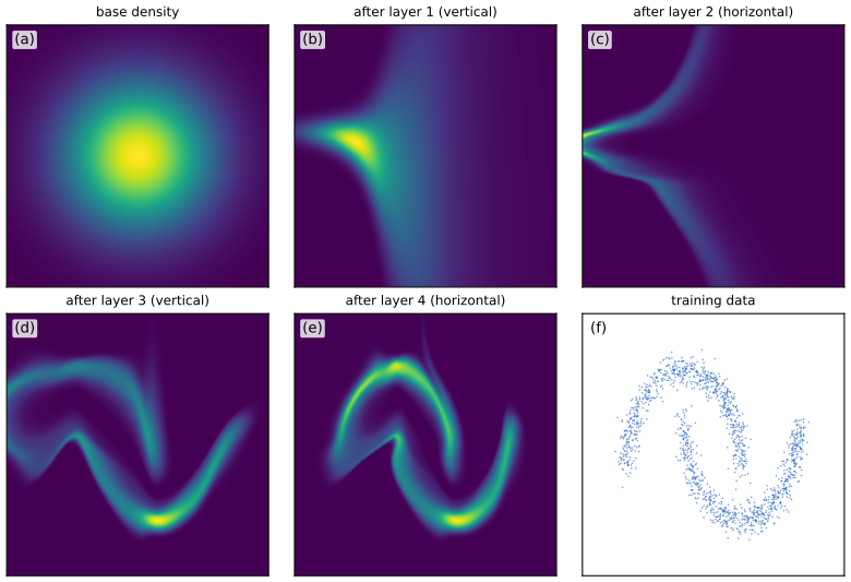
Panel (b) is Result 18.2(4) in a picture: after one vertical layer each column \(x_1=\text{const}\) holds a Gaussian whose centre and width depend on \(x_1\). The horizontal layer then moves rows, and so on.
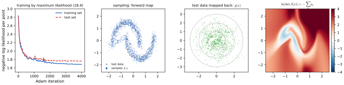
Filling the gap 18.4: the sign of the log-determinant, and why the moons stay connected Figure 18.3
Derivation
Reading Figure 18.S1(d). From (18.1), \(\ln p_\bx(\bx)=\ln p_\bz(\bz)+\ln|\det\bJ|\). On the moons \(p_\bx\) is high, but \(\bz=\bg(\bx)\) ranges over the whole base Gaussian, so the log-determinant must make up the difference: it is large where the flow compresses base volume into a small data region (\(|\det\bJ|>1\)) and small where it spreads base volume out. Away from the data the inverse squeezes large regions of \(\bx\) into the tails of the base, \(|\det\bJ|\) is large there too, but \(p_\bz(\bz)\) is tiny, so the product is small.
Topology. \(\bf\) is a homeomorphism of \(\R^2\), so the support of the model is all of \(\R^2\) and the density is positive everywhere; a flow cannot produce two components separated by a region of exactly zero density. It can only make the density very small in the gap, which requires very large local stretching (large \(|s|\)). This is why the trained density of Figure 18.3(e) keeps a thin bridge between the moons and why deeper flows fit such data better. The same argument shows that a continuous flow (Section 18.3) cannot change the topology either. ∎
18.2 Autoregressive Flows
See also Chapter 11 of these notes, factorization; the companion course, autoregressive models and Section 8.1.
pp. 552–553 Any joint distribution factorises along an ordering of the variables, without loss of generality:
\[ p(x_1,\dots,x_D)=\prod_{i=1}^Dp(x_i\given\bx_{1:i-1}). \tag{18.16} \]A masked autoregressive flow (MAF; Papamakarios, Pavlakou and Murray, 2017) builds each variable from its own latent variable and the variables before it,
\[ x_i=h(z_i,g_i(\bx_{1:i-1},\bw_i)), \tag{18.17} \]with a coupling function \(h(\cdot,g)\) invertible in its first argument and a conditioner \(g_i\). "Masked" refers to implementing all \(D\) conditioners with one network whose weights are multiplied by binary masks (Germain et al., 2015; Filling the gap 18.5). Density evaluation inverts (18.17):
\[ z_i=h^{-1}(x_i,g_i(\bx_{1:i-1},\bw_i)), \tag{18.18} \]and since \(\bx\) is known, all \(D\) equations can be evaluated at once. Sampling must follow (18.17) in order: \(x_i\) needs \(x_1,\dots,x_{i-1}\) first. The inverse autoregressive flow (IAF; Kingma et al., 2016) conditions on the latent variables instead,
\[ x_i=h(z_i,\tilde g_i(\bz_{1:i-1},\bw_i)), \tag{18.19} \]so that sampling is parallel and density evaluation sequential:
\[ z_i=h^{-1}(x_i,\tilde g_i(\bz_{1:i-1},\bw_i)). \tag{18.20} \]Definition 18.2 (affine MAF and IAF) pp. 552–554, (18.17)–(18.20)
With the affine coupling function \(h(z,(\mu,\alpha))=\mu+e^{\alpha}z\) and a network that returns \((\mu_i,\alpha_i)\) depending only on the first \(i-1\) entries of its input \(\bu\):
- MAF (input \(\bu=\bx\)): \(x_i=\mu_i(\bx_{1:i-1})+e^{\alpha_i(\bx_{1:i-1})}z_i\); inverse \(z_i=(x_i-\mu_i)e^{-\alpha_i}\).
- IAF (input \(\bu=\bz\)): \(x_i=\mu_i(\bz_{1:i-1})+e^{\alpha_i(\bz_{1:i-1})}z_i\); inverse \(z_i=(x_i-\mu_i(\bz_{1:i-1}))e^{-\alpha_i(\bz_{1:i-1})}\).
Result 18.3 (triangular Jacobian and the cost of each direction) pp. 553–554; Exercise 18.4
- For both MAF and IAF, \(\partial z_i/\partial x_j=0\) for \(j>i\): the Jacobian \(\bJ\) of \(\bx\mapsto\bz\) is lower triangular with diagonal \(e^{-\alpha_i}\), and \(\ln p(\bx)=\sum_i\ln\N(z_i\given0,1)-\sum_i\alpha_i\).
- For an affine MAF this is the Gaussian autoregressive model \(p(\bx)=\prod_i\N\big(x_i\given\mu_i(\bx_{1:i-1}),e^{2\alpha_i(\bx_{1:i-1})}\big)\), a model of the form (18.16).
- Counting sequential network passes:
| density of a given \(\bx\) | draw a sample | |
|---|---|---|
| MAF | 1 pass (input \(\bx\) known) | \(D\) passes |
| IAF | \(D\) passes | 1 pass, and the sample's density is free |
| coupling layer | 1 pass | 1 pass |
Proof
(1) MAF: \(z_i=(x_i-\mu_i(\bx_{1:i-1}))e^{-\alpha_i(\bx_{1:i-1})}\) depends only on \(x_1,\dots,x_i\), so \(\partial z_i/\partial x_j=0\) for \(j>i\), and \(\partial z_i/\partial x_i=e^{-\alpha_i}\) because \(\mu_i,\alpha_i\) do not involve \(x_i\). IAF: by induction on \(i\), \(z_i\) is a function of \(x_1,\dots,x_i\) only (true for \(i=1\), where \(\mu_1,\alpha_1\) are constants; if true up to \(i-1\), then \(\mu_i(\bz_{1:i-1})\) and \(\alpha_i(\bz_{1:i-1})\) depend on \(\bx_{1:i-1}\), and \(z_i\) on \(\bx_{1:i}\)), and again \(\partial z_i/\partial x_i=e^{-\alpha_i}\). By Filling the gap 18.3, \(\ln|\det\bJ|=-\sum_i\alpha_i\), and (18.1) gives the formula. (The book calls this matrix upper triangular on p. 553; with \(J_{ij}=\partial z_i/\partial x_j\) as in (18.2) it is lower triangular, as Exercise 18.4 states.)
(2) \(\ln\N(z_i\given0,1)-\alpha_i\)
(3) A pass of the network needs its whole input vector. In the MAF density and the IAF sample the input (\(\bx\), resp. \(\bz\)) is known, so one pass returns every \((\mu_i,\alpha_i)\). In the MAF sample the input \(\bx\) is the unknown being built: pass \(i\) can only be run once \(x_1,\dots,x_{i-1}\) are known, and it yields \(x_i\); \(D\) passes in sequence (the IAF density is the same with \(\bz\)). When the IAF draws a sample, \(\bz\) and all \(\alpha_i\) are at hand, so \(\ln p\) of that sample costs nothing extra; only points that it did not generate are expensive. A coupling layer conditions on a block that is known in both directions. ∎
A direct computation verifies the triangular pattern and the diagonal by finite differences, the round trips (\(4\times10^{-16}\)), that the free IAF density of a sample equals the \(D\)-pass evaluation, and that both models are normalised but different densities. Figure 18.S2 times the four operations.
Filling the gap 18.5: how masks make one network autoregressive p. 553; Germain et al. (2015)
The book says a binary mask forces some weights to zero to implement (18.16). Here is the construction used in the demo and the code, and a proof that it works.
Derivation
Construction (one hidden layer). Give input \(d\) the degree \(d\in\{1,\dots,D\}\) and hidden unit \(k\) a degree \(m_k\in\{1,\dots,D-1\}\). Keep the weight from input \(d\) to unit \(k\) only if \(m_k\ge d\) (mask \(M^{(1)}_{kd}=\Ind[m_k\ge d]\)), and from unit \(k\) to output \(i\) (both \(\mu_i\) and \(\alpha_i\)) only if \(i>m_k\) (mask \(M^{(2)}_{ik}=\Ind[i>m_k]\)). The network is \(\bh=\tanh((\mathbf W^{(1)}\odot\mathbf M^{(1)})\bu+\bb^{(1)})\), \((\bmu,\balpha)=(\mathbf W^{(2)}\odot\mathbf M^{(2)})\bh+\bb^{(2)}\).
Claim. \(\mu_i\) and \(\alpha_i\) do not depend on \(u_j\) for \(j\ge i\). Proof: a dependence requires a path \(j\to k\to i\) with both weights kept, i.e. \(j\le m_k<i\), so \(j<i\). Equivalently, the matrix \(\mathbf M^{(2)}\mathbf M^{(1)}\), whose \((i,j)\) entry counts such paths, is strictly lower triangular. With several hidden layers the degrees must be non-decreasing along each kept connection (\(m^{(l+1)}_k\ge m^{(l)}_{k'}\)), and the same argument applies along any path.
Expressiveness. Output \(i\) can see every input \(j<i\) as long as some hidden unit has degree \(m\) with \(j\le m<i\); choosing \(m_k=1+(k\bmod(D-1))\) with at least \(D-1\) hidden units ensures this. Output 1 sees nothing: \(\mu_1,\alpha_1\) are biases. A single pass then computes all \(D\) conditionals of (18.16), which a naive implementation would compute with \(D\) separate networks.
Coupling flows are a special case. Take two blocks instead of \(D\) variables: \(\bx_A\) with \(\bmu=\bzero\), \(\balpha=\bzero\), and \(\bx_B\) conditioned on \(\bx_A\). That is (18.10)–(18.11): a coupling layer is an autoregressive layer with two groups, which trades generality for one-pass computation in both directions (p. 554). ∎
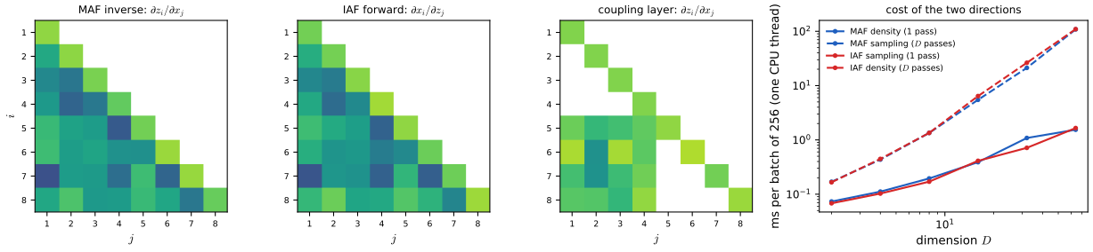
p. 554 Which of MAF or IAF to prefer depends on the use. MAF suits density estimation (training by maximum likelihood on data needs fast density evaluation); IAF suits settings where the model generates its own samples and needs their densities, such as a flexible approximate posterior in a variational autoencoder (Kingma et al., 2016). Both pay a cost linear in \(D\) for one of the two directions; coupling flows sacrifice some flexibility to be fast in both.
18.3 Continuous Flows
p. 554 The last construction defines the network by an ordinary differential equation, a network with infinitely many layers. Section 18.3.1 introduces neural ODEs, Section 18.3.2 their training, and Section 18.3.3 the resulting flows.
18.3.1 Neural differential equations
See also Chapter 9 of these notes, residual connections.
pp. 554–555 A residual network with the same function in every layer,
\[ \bz^{(t+1)}=\bz^{(t)}+\bf(\bz^{(t)},\bw), \tag{18.21} \]for \(t=1,\dots,T\), becomes in the limit of many small steps the neural ODE (Chen et al., 2018)
\[ \frac{\d\bz(t)}{\d t}=\bf(\bz(t),\bw), \tag{18.22} \]whose output is obtained by integration. The book writes \(\bz(T)=\int_0^T\bf(\bz(t),\bw)\,\d t\); the initial value is missing, and the correct statement is
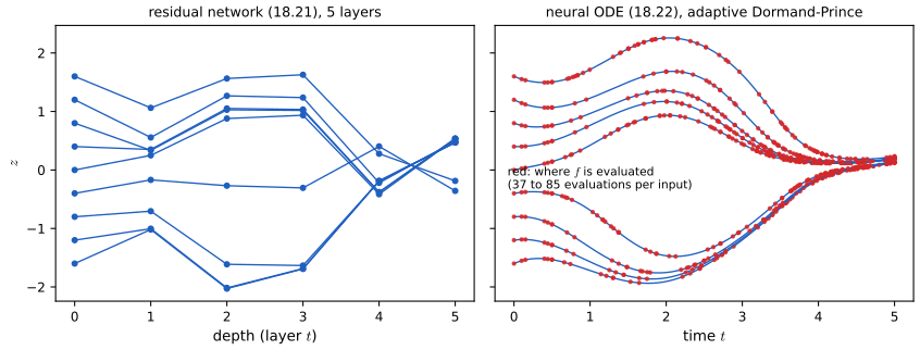
\[ \bz(T)=\bz(0)+\int_0^T\bf(\bz(t),\bw)\,\d t. \tag{18.23} \]Euler's method with unit step is exactly (18.21); adaptive solvers choose the evaluation times to meet an error tolerance, and the number of evaluations plays the role of depth (Figure 18.5). Everything below also holds for \(\bf(\bz,t,\bw)\) with explicit time dependence.
Result 18.4 (residual networks converge to the ODE; the flow map is a diffeomorphism) pp. 554–555; Exercise 18.5
Assume \(\bf(\bz,t)\) is continuous, continuously differentiable in \(\bz\), and globally Lipschitz in \(\bz\) with constant \(L\) (true for a tanh network: \(L\le\prod_l\|\mathbf W^{(l)}\|_2\)).
- (18.22) has a unique solution on \([0,T]\) for every \(\bz(0)\) (Picard–Lindelöf).
- The residual network \(\bz_{k+1}=\bz_k+\epsilon\bf(\bz_k,k\epsilon)\) (18.38) with \(\epsilon=T/n\) satisfies \(\max_k\|\bz_k-\bz(k\epsilon)\|=O(\epsilon)\).
- The flow map \(\phi_T:\bz(0)\mapsto\bz(T)\) is a diffeomorphism; its inverse is obtained by integrating (18.22) backwards from \(T\) to 0, and \(\det\partial\phi_T/\partial\bz(0)>0\).
- Solution curves never cross; in one dimension \(\phi_T\) is strictly increasing.
Proof
(1) Standard: the Picard map \(\bz(\cdot)\mapsto\bz(0)+\int_0^t\bf(\bz(s),s)\d s\) is a contraction in the norm \(\sup_te^{-2Lt}\|\bz(t)\|\), so it has a unique fixed point.
(2) The local error of one Euler step is \(\bz(t+\epsilon)-\bz(t)-\epsilon\bf(\bz(t),t)=\frac{\epsilon^2}2\ddot\bz(\xi)\) (componentwise, by Taylor), bounded by \(C\epsilon^2\) since \(\ddot\bz=\partial_t\bf+(\partial\bf/\partial\bz)\bf\) is bounded on the compact trajectory. With \(\mathbf e_k=\bz_k-\bz(k\epsilon)\), \(\|\mathbf e_{k+1}\|\le(1+L\epsilon)\|\mathbf e_k\|+C\epsilon^2\), so \(\|\mathbf e_k\|\le C\epsilon^2\sum_{j<k}(1+L\epsilon)^j\le\frac{C\epsilon}{L}(e^{LT}-1)\). Dividing (18.38) by \(\epsilon\) shows the formal limit: \((\bz(t+\epsilon)-\bz(t))/\epsilon=\bf\to\d\bz/\d t\) (Exercise 18.5).
(3) By uniqueness, the solution through \(\bz(T)\) run backwards returns to \(\bz(0)\), so \(\phi_T\) is a bijection with inverse the backward flow, and both are continuously differentiable (differentiable dependence on initial conditions). Its Jacobian \(\bM(t)=\partial\bz(t)/\partial\bz(0)\) solves \(\dot\bM=(\partial\bf/\partial\bz)\bM\), \(\bM(0)=\bI\), and by Jacobi's formula (Result 18.6) \(\det\bM(T)=\exp\int_0^T\Tr(\partial\bf/\partial\bz)\d t>0\).
(4) If two solutions met at a time \(t^\star\), both would solve the same initial value problem from \(t^\star\) backwards and would coincide for all \(t\). In one dimension, two solutions that start ordered stay ordered, so \(\phi_T\) is increasing; a neural ODE on \(\R\) cannot represent \(x\mapsto-x\), and in general it preserves orientation. ∎
Numerical experiments confirm the \(O(\epsilon)\) rate (error ratios 2.03, 2.01, 2.01 as \(\epsilon\) halves), the \(O(h^4)\) rate of the Runge–Kutta method used in the demos (ratios 15.8, 16.0), the inverse by backward integration (\(2\times10^{-11}\)), and that the five-layer residual network of Figure 18.5 has crossing trajectories while the ODE's are ordered at every \(t\).
18.3.2 Neural ODE backpropagation
See also Chapter 8 of these notes, evaluation of gradients and reverse-mode automatic differentiation; Chapter 9, parameter sharing.
pp. 555–557 To train, we need \(\nabla_\bw L\) for a loss \(L\) of the output \(\bz(T)\). Differentiating through the solver's operations works but stores every intermediate state and differentiates the solver's discretisation rather than the ODE. Chen et al. (2018) use the adjoint sensitivity method, the continuous analogue of backpropagation's three phases (forward pass, backward pass for the activations, products for the weights). The adjoint is
\[ \ba(t)=\frac{\d L}{\d\bz(t)}, \tag{18.24} \]so \(\ba(T)\) is the ordinary output gradient. It satisfies
\[ \frac{\d\ba(t)}{\d t}=-\ba(t)^\T\nabla_\bz\bf(\bz(t),\bw), \tag{18.25} \]integrated backwards from \(\ba(T)\) with \(\bz(t)\) recomputed alongside it by running (18.22) backwards from \(\bz(T)\). Because \(\bw\) is shared by all "layers", its gradient sums (integrates) the contributions of every time. The book writes this as \(\nabla_\bw L=-\int_0^T\ba^\T\nabla_\bw\bf\,\d t\), with the sign wrong; the correct formula is
\[ \nabla_\bw L=\int_0^T\ba(t)^\T\nabla_\bw\bf(\bz(t),\bw)\,\d t\;\Big({=}-\int_T^0\ba(t)^\T\nabla_\bw\bf\,\d t\Big). \tag{18.26} \]Result 18.5 (the adjoint method) (18.24)–(18.26); Exercises 18.6, 18.7
Under the assumptions of Result 18.4, with \(\bf\) also continuously differentiable in \(\bw\), and \(L\) differentiable: \(\ba(t)^\T\) solves (18.25) with \(\ba(T)^\T=\partial L/\partial\bz(T)\), \(\ba(0)=\d L/\d\bz(0)\), and \(\nabla_\bw L\) is given by (18.26) with a plus sign. Equivalently, integrate the augmented system \((\bz,\ba,\mathbf g)\) from \(t=T\) to \(t=0\): \[ \dot\bz=\bf,\qquad\dot\ba^\T=-\ba^\T\frac{\partial\bf}{\partial\bz},\qquad\dot{\mathbf g}^\T=-\ba^\T\frac{\partial\bf}{\partial\bw},\qquad\mathbf g(T)=\bzero, \] and read off \(\nabla_\bw L=\mathbf g(0)\). The memory cost does not grow with the number of solver steps.
Proof
The adjoint equation. Let \(\phi_{s\leftarrow t}\) map the state at time \(t\) to the state at time \(s\). Then \(L=\ell(\phi_{T\leftarrow t}(\bz(t)))\) for every \(t\), and \(\phi_{T\leftarrow t}=\phi_{T\leftarrow t+h}\circ\phi_{t+h\leftarrow t}\). By the chain rule, \[ \ba(t)^\T=\ba(t+h)^\T\frac{\partial\bz(t+h)}{\partial\bz(t)}=\ba(t+h)^\T\Big(\bI+h\frac{\partial\bf}{\partial\bz}(\bz(t))+O(h^2)\Big). \] Rearranging, \(\frac{\ba(t+h)^\T-\ba(t)^\T}{h}=-\ba(t+h)^\T\frac{\partial\bf}{\partial\bz}+O(h)\), and \(h\to0\) gives (18.25). At \(t=0\) the definition gives \(\ba(0)=\d L/\d\bz(0)\).
The weight gradient. Treat \(\bw\) as extra state with \(\dot\bw=\bzero\), so the augmented state \(\hat\bz=(\bz,\bw)\) has velocity \(\hat\bf=(\bf,\bzero)\) and Jacobian \(\partial\hat\bf/\partial\hat\bz=\begin{bmatrix}\partial\bf/\partial\bz&\partial\bf/\partial\bw\\ \bzero&\bzero\end{bmatrix}\). Its adjoint \(\hat\ba=(\ba,\ba_\bw)\) obeys (18.25): \(\dot\ba^\T=-\ba^\T\partial\bf/\partial\bz\) and \(\dot\ba_\bw^\T=-\ba^\T\partial\bf/\partial\bw\). At the final time \(L\) does not depend on the \(\bw\)-component of the state directly, so \(\ba_\bw(T)=\bzero\), while \(\ba_\bw(0)=\d L/\d\bw\) (the initial \(\bw\)-state is the parameter). Integrating, \[ \nabla_\bw L=\ba_\bw(0)=\ba_\bw(T)-\int_0^T\dot\ba_\bw\,\d t=\int_0^T\ba(t)^\T\frac{\partial\bf}{\partial\bw}\,\d t. \] The sign is plus. The discrete version makes it transparent (Exercise 18.7): for (18.38), \(\partial L/\partial\bw=\sum_k\epsilon\,\ba_{k+1}^\T\partial\bf/\partial\bw(\bz_k)\), a sum of positive multiples of the per-layer contributions, whose limit is (18.26) with \(+\). Chen et al. (2018) write \(-\int_{t_1}^{t_0}\), integrating from the final time back to the initial one, which is the same thing; the book keeps their minus sign with the limits in the forward order.
Memory. The backward integration needs \(\bz(t)\) at the times the solver chooses; it recomputes them from \(\bz(T)\) instead of storing them, so the memory does not depend on the number of steps. ∎
Both versions were implemented: the discrete adjoint of a 20-layer residual network equals automatic differentiation to \(4\times10^{-16}\) (Exercises 18.6–18.7); the continuous adjoint (RK4 backwards, state recomputed) matches finite differences of the loss for all 42 weights to \(1.6\times10^{-9}\), while the book's sign gives the negative gradient.
Algorithm 18.2 (gradient of a neural ODE by the adjoint method) pp. 555–557
- Forward: solve (18.22) from \(\bz(0)\) to \(\bz(T)\) with any solver; keep only \(\bz(T)\).
- Set \(\ba(T)=\nabla_{\bz(T)}L\), \(\mathbf g=\bzero\).
- Solve the augmented system of Result 18.5 from \(T\) back to 0. Each evaluation needs \(\bf\) and the two vector-Jacobian products \(\ba^\T\partial\bf/\partial\bz\) and \(\ba^\T\partial\bf/\partial\bw\), one reverse-mode pass through the network.
- Return \(\nabla_\bw L=\mathbf g(0)\) and \(\nabla_{\bz(0)}L=\ba(0)\). If the loss depends on several intermediate times \(t_1<\dots<t_K\), run the backward solve piecewise between them, adding \(\partial L/\partial\bz(t_k)\) to \(\ba\) at each \(t_k\).
Filling the gap 18.6: when the adjoint is inexact, and what it costs pp. 556–557
Derivation
Two different gradients. Backpropagation through the solver gives the exact gradient of the discretised loss; the adjoint method gives a discretisation of the gradient of the exact loss. They differ by the solver error. For RK4 both errors are \(O(h^4)\) (Figure 18.S3(c): the two curves are parallel with slope 4), while a residual network trained by exact backpropagation is the Euler discretisation and converges to the ODE gradient only at rate \(O(h)\).
Backward reconstruction can be unstable. Recomputing \(\bz(t)\) backwards assumes the backward flow is well conditioned. For \(\dot z=-\lambda z\) with \(\lambda>0\), a perturbation \(\delta\) of \(z(T)\) becomes \(\delta e^{\lambda T}\) at \(t=0\): a strongly contracting forward flow (which is what a flow does where it concentrates mass) is strongly expanding backwards, and rounding errors in the reconstructed state grow accordingly. Storing checkpoints of \(\bz\) during the forward pass, at a memory cost, removes the problem.
Cost. Each backward evaluation costs one forward and one reverse pass of the network, so the backward solve costs about two to three times the forward solve, independent of the memory saving. ∎
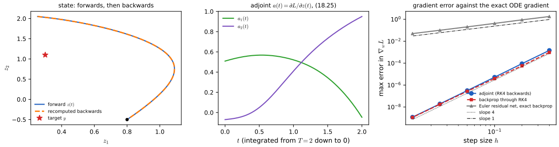
p. 557 Two further advantages: neural ODEs handle observations at arbitrary times (losses at several times need the piecewise backward solve of Algorithm 18.2), and the solver tolerance can be loosened at inference time, trading accuracy for fewer function evaluations.
18.3.3 Neural ODE flows
See also the companion course, Result 11.24 (Hamiltonian flows have zero divergence and preserve volume) and Toolkit, Result T.8 (expected quadratic forms).
pp. 557–558 A neural ODE
\[ \frac{\d\bz(t)}{\d t}=\bf(\bz(t),\bw) \tag{18.27} \]is a flexible invertible map from \(\bz(0)\) to \(\bz(T)\), so a base density \(p(\bz(0))\) induces densities \(p(\bz(t))\) for all \(t\). Chen et al. (2018) showed that the log density changes along each path at the rate
\[ \frac{\d\ln p(\bz(t))}{\d t}=-\Tr\Big(\frac{\partial\bf}{\partial\bz(t)}\Big). \tag{18.28} \]This is a continuous normalizing flow: sample by integrating (18.27) from a base draw; evaluate a density by integrating (18.27) backwards from \(\bx\) to \(\bz(0)\) while accumulating the trace. The derivative in (18.28) is the derivative along the path (the total derivative), not the partial derivative at a fixed point.
Result 18.6 (the instantaneous change of variables) (18.28); Exercises 18.8–18.10
Under the assumptions of Result 18.4, let \(\bM(t)=\partial\bz(t)/\partial\bz(0)\) and \(p_t\) be the density of \(\bz(t)\). Then
- (Jacobi's formula) \(\dfrac{\d}{\d t}\ln\det\bM(t)=\Tr\Big(\dfrac{\partial\bf}{\partial\bz}(\bz(t),t)\Big)\), so \(\det\bM(T)=\exp\int_0^T\Tr(\partial\bf/\partial\bz)\,\d t\);
- \(\ln p_T(\bz(T))\)
\({}=\ln p_0(\bz(0))\) \({}-\int_0^T\Tr\big(\partial\bf/\partial\bz\big)\d t\), and differentiating in \(T\) gives (18.28); - equivalently, \(p_t\) satisfies the continuity equation \(\partial_tp+\nabla\cdot(p\bf)=0\), of which (18.28) is the form along paths;
- a velocity field with zero divergence preserves volume and density along paths (Hamiltonian dynamics is the classic example).
Proof
(1) Differentiating (18.27) with respect to \(\bz(0)\) gives the variational equation \(\dot\bM=\bA(t)\bM\), \(\bA=\partial\bf/\partial\bz\), \(\bM(0)=\bI\). For small \(h\), \(\bM(t+h)=(\bI+h\bA+O(h^2))\bM(t)\), and \(\det(\bI+h\bA)=1+h\Tr\bA+O(h^2)\) (expand the determinant: every product other than the diagonal one contains at least two off-diagonal entries, each \(O(h)\)). Hence \(\det\bM(t+h)\)
(2) Apply (18.34) to the flow map: \(p_T(\bz(T))=p_0(\bz(0))\,|\det\bM(T)|^{-1}\), take logarithms and use (1).
(3) For a smooth test function \(\varphi\), \(\E[\varphi(\bz(t))]=\int\varphi\,p_t\), and its time derivative is \(\E[\nabla\varphi\cdot\bf]=\int p_t\bf\cdot\nabla\varphi=-\int\varphi\,\nabla\cdot(p_t\bf)\) (integration by parts, with decay at infinity). Comparing with \(\int\varphi\,\partial_tp_t\) gives the continuity equation. Along a path, \[ \frac{\d}{\d t}\ln p_t(\bz(t))=\frac{\partial_tp+\bf\cdot\nabla p}{p}=\frac{-\nabla\cdot(p\bf)+\bf\cdot\nabla p}{p}=-\nabla\cdot\bf, \] and \(\nabla\cdot\bf=\Tr(\partial\bf/\partial\bz)\).
(4) If \(\Tr(\partial\bf/\partial\bz)\equiv0\), (1) gives \(\det\bM\equiv1\) and (2) gives \(p_T(\bz(T))=p_0(\bz(0))\). ∎
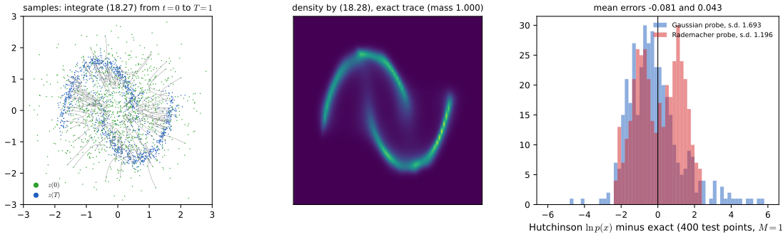
Numerical experiments confirm (1) exactly for a linear ODE (\(\ln\det=T\Tr\bA\) to \(10^{-12}\)) and, for the trained flow of Figure 18.S5, that \(\int_0^1\Tr\) equals \(\ln|\det|\) of the finite-difference Jacobian of the whole flow map to \(3\times10^{-9}\).
Filling the gap 18.7: the one-dimensional picture and the flow lines of Figure 18.6 Exercises 18.8, 18.9
Derivation
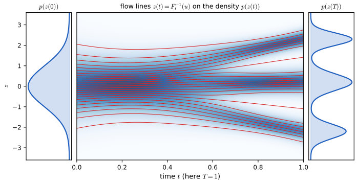
Mass in an interval. In one dimension let \(F_t(z)=\int_{-\infty}^zp_t\) be the distribution function. A path \(z(t)\) of (18.27) carries a fixed amount of mass below it, because paths cannot cross (Result 18.4(4)): \(F_t(z(t))=u\) is constant. Differentiating, \(p_t(z)\dot z+\partial_tF_t(z)=0\), so the velocity must be \[ f(z,t)=-\frac{\partial_tF_t(z)}{p_t(z)}. \] Conversely, given any smooth family \(p_t\) with \(p_t>0\), this \(f\) moves the quantile \(z(t)=F_t^{-1}(u)\) along a path of (18.27). So the flow lines of Figure 18.6, drawn as quantiles of \(p_t\) for equally spaced \(u\), are exactly the solutions of (18.27) with this \(f\) (Exercise 18.9). Differentiating \(\partial_tF+fp=0\) in \(z\) gives \(\partial_tp+\partial_z(fp)=0\), the one-dimensional continuity equation, and hence (18.28).
Uniqueness in 1-D. The continuity equation determines \(fp\) up to a function of \(t\) alone, which must vanish if \(fp\to0\) as \(z\to-\infty\); so in one dimension the velocity field generating a given \(p_t\) is unique. (In two or more dimensions it is not: adding any field \(\mathbf v\) with \(\nabla\cdot(p\mathbf v)=0\), such as a rotation of a radially symmetric density, leaves \(p_t\) unchanged.)
Figure 18.6. The path used is the law of \((1-t)z_0+tx_1\) with \(z_0\sim\N(0,1)\) and \(x_1\) from a three-component mixture, so \(p_t=\sum_k\pi_k\N(tm_k,(1-t)^2+t^2s_k^2)\): Gaussian at \(t=0\), the mixture at \(t=T=1\). Its \(F_t\) and \(\partial_tF_t\) are sums of normal distribution functions and densities, so \(f\) is available in closed form. Numerically, integrating \(\dot z=f\) from five quantiles of \(p_0\) lands on the same quantiles of \(p_1\) to \(10^{-9}\), (18.39) holds along the lines, and this \(f\) equals the flow-matching velocity of Filling the gap 18.8 (\(9\times10^{-16}\)), as uniqueness demands. Where lines spread apart \(f'>0\) and the density falls; where they converge it rises. ∎
pp. 557–558 A trace looks cheaper than a determinant, \(O(D)\) against \(O(D^3)\) once the matrix is known, but forming the diagonal of \(\partial\bf/\partial\bz\) for a general network takes \(D\) passes (one vector-Jacobian product per row), so the exact trace costs \(D\) network evaluations per function evaluation. Hutchinson's estimator (Hutchinson, 1989; used for flows by Grathwohl et al., 2018) avoids this: for a random vector \(\beps\) with \(\E[\beps\beps^\T]=\bI\),
\[ \Tr(\bA)=\E_\beps\big[\beps^\T\bA\beps\big], \tag{18.29} \] \[ \Tr(\bA)\simeq\frac1M\sum_{m=1}^M\beps_m^\T\bA\beps_m, \tag{18.30} \]and \(\beps^\T\bA\) is one reverse-mode pass. In practice \(M=1\), with a new probe for each data point, held fixed along that point's path.
Result 18.7 (Hutchinson's estimator: bias and variance) (18.29)–(18.30); Exercise 18.11
- If \(\E[\beps\beps^\T]=\bI\) (zero mean is not needed), (18.30) is unbiased for every \(M\).
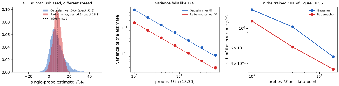
- Let \(\bS=\frac12(\bA+\bA^\T)\) and let \(\beps\) have independent coordinates with mean 0, variance 1 and fourth moment \(\mu_4\). Then \[ \var\big[\beps^\T\bA\beps\big]=2\|\bS\|_F^2+(\mu_4-3)\sum_iS_{ii}^2, \] and (18.30) has variance \(1/M\) times this. Gaussian probes (\(\mu_4=3\)): \(2\|\bS\|_F^2\). Rademacher probes (\(\pm1\), \(\mu_4=1\)): \(2\big(\|\bS\|_F^2-\sum_iS_{ii}^2\big)\), the smallest possible among such probes, and zero for a diagonal matrix.
- In a continuous flow with a probe held fixed along the path, the estimate of \(\ln p(\bx)\) is unbiased, but \(\exp\) of it overestimates \(p(\bx)\) on average (Jensen's inequality).
Proof
(1) \(\E[\beps^\T\bA\beps]\)
(2) \(\beps^\T\bA\beps=\beps^\T\bS\beps\) since the antisymmetric part contributes zero. For independent coordinates with mean 0 and variance 1, \[ \E[\epsilon_i\epsilon_j\epsilon_k\epsilon_l]=\delta_{ij}\delta_{kl}+\delta_{ik}\delta_{jl}+\delta_{il}\delta_{jk}+(\mu_4-3)\delta_{ijkl} \] (check the cases: all four indices equal gives \(\mu_4\); two distinct pairs give 1; anything else 0). Then \[ \E[(\beps^\T\bS\beps)^2]=\sum_{ijkl}S_{ij}S_{kl}\E[\epsilon_i\epsilon_j\epsilon_k\epsilon_l]=(\Tr\bS)^2+2\sum_{ij}S_{ij}^2+(\mu_4-3)\sum_iS_{ii}^2, \] and subtracting \((\Tr\bS)^2\) gives the variance. Since \(\mu_4\ge(\E\epsilon^2)^2=1\) with equality only if \(\epsilon^2=1\) almost surely, Rademacher probes minimise the variance in this class. Independent probes divide the variance by \(M\).
(3) Along the path the estimate of \(\int_0^T\Tr\) is \(\int_0^T\beps^\T\bA(t)\beps\,\d t\), whose expectation is \(\int\Tr\bA\) by (1) and Fubini; \(\ln\hat p=\ln p_0(\bz(0))-\int\beps^\T\bA\beps\) is therefore unbiased. As \(\exp\) is strictly convex, \(\E[\hat p]=\E[e^{\ln\hat p}]>e^{\E\ln\hat p}=p\) unless the estimate is exact. ∎
Numerical experiments enumerate all 64 Rademacher probes in \(D=6\) (mean equals \(\Tr\bA\) to \(10^{-12}\), variance equals the formula), confirm the Gaussian and uniform (\(\mu_4=9/5\)) cases by simulation, and confirm (3) on the trained flow: over \(20\times300\) estimates the error in \(\ln p\) has mean \(-0.006\) (standard error 0.016) and standard deviation 1.21, while the average estimated density is twice the exact one.
Algorithm 18.3 (sampling and density evaluation in a continuous flow) pp. 557–558, (18.27)–(18.30)
- Sample: draw \(\bz(0)\sim\N(\bzero,\bI)\); integrate (18.27) from 0 to \(T\); output \(\bz(T)\). To also get its density, integrate \(\ell'=-\Tr(\partial\bf/\partial\bz)\) alongside, from \(\ell(0)=\ln\N(\bz(0)\given\bzero,\bI)\).
- Density of a given \(\bx\): set \(\bz(T)=\bx\), \(c=0\); integrate backwards from \(T\) to 0 the pair \(\dot\bz=\bf\), \(\dot c=\Tr(\partial\bf/\partial\bz)\) (or \(\beps^\T(\partial\bf/\partial\bz)\beps\) with one probe \(\beps\) fixed along the path); then \(\ln p(\bx)=\ln\N(\bz(0)\given\bzero,\bI)+c(0)\), where \(c(0)=-\int_0^T\Tr\,\d t\).
- Both directions cost the same number of function evaluations (Exercise 18.10). Training by maximum likelihood differentiates step 2 with the adjoint method of Algorithm 18.2 applied to the augmented state \((\bz,c)\).
p. 558 The book closes with flow matching (Lipman et al., 2022), which trains continuous flows far more efficiently, without backpropagating through the integrator, and links them to diffusion models (Chapter 20 of the book). The flow of Figure 18.S5 and of the demo was trained this way.
Filling the gap 18.8: flow matching in one page p. 558, beyond the book
The book only names flow matching. Here is the idea and the one identity that makes it work.
Derivation
A path of densities with a known velocity. Pair a base draw \(\bz_0\sim\N(\bzero,\bI)\) with a data point \(\bx_1\) and move in a straight line, \(\bz_t=(1-t)\bz_0+t\bx_1\), whose velocity is \(\bx_1-\bz_0\). The law \(p_t\) of \(\bz_t\) is Gaussian at \(t=0\) and the data distribution at \(t=1\). The marginal velocity \(\mathbf u(\bz,t)=\E[\bx_1-\bz_0\given\bz_t=\bz]\) generates \(p_t\): for a test function \(\varphi\), \[ \frac{\d}{\d t}\E\varphi(\bz_t)=\E[\nabla\varphi(\bz_t)\cdot(\bx_1-\bz_0)]=\E[\nabla\varphi(\bz_t)\cdot\mathbf u(\bz_t,t)] \] by the tower property, which is the weak form of \(\partial_tp+\nabla\cdot(p\mathbf u)=0\). So the ODE (18.27) with \(\bf=\mathbf u\) carries \(\N(\bzero,\bI)\) to the data, and (18.28) gives its density.
Regression without knowing \(\mathbf u\). \(\mathbf u\) involves an intractable conditional expectation, but for any network \(\mathbf v(\bz,t)\), \[ \E\big\|\mathbf v(\bz_t,t)-(\bx_1-\bz_0)\big\|^2=\E\big\|\mathbf v(\bz_t,t)-\mathbf u(\bz_t,t)\big\|^2+\E\big\|\mathbf u(\bz_t,t)-(\bx_1-\bz_0)\big\|^2, \] because the cross term \(2\E[(\mathbf v-\mathbf u)\cdot(\mathbf u-(\bx_1-\bz_0))]\) vanishes after conditioning on \((\bz_t,t)\). The second term does not involve \(\mathbf v\). So minimising the simple conditional loss on the left (sample \(t\sim\Unif(0,1)\), \(\bz_0\), \(\bx_1\); regress) has the same gradients as regressing on the unknown \(\mathbf u\). No ODE is solved during training; the integrator is only used to sample and to evaluate densities.
In practice here. A tanh network with 32 units per layer, trained for 20 000 Adam steps on the two moons (about 40 s on one CPU thread), gives a test log likelihood of \(-1.79\) per point (the real NVP of Figure 18.3: \(-1.76\)), the same with 20 or 80 Runge–Kutta steps, and a density whose mass on \([-3,3]^2\) is 1.0000. In one dimension a direct computation confirms the decomposition: the conditional loss minus the marginal loss is the same constant (2.58) for three different \(\mathbf v\). ∎
Summary: errors and imprecisions found in the chapter (first printing)
- p. 553: the Jacobian \(\partial z_i/\partial x_j\) of (18.18) is called "upper-triangular". Since \(z_i\) depends only on \(x_1,\dots,x_i\), the entries with \(j>i\) vanish and the matrix is lower triangular, as Exercise 18.4 says (checked by finite differences, Result 18.3).
- (18.23): \(\bz(T)=\int_0^T\bf\,\d t\) omits the initial value; it should be \(\bz(T)=\bz(0)+\int_0^T\bf\,\d t\).
- (18.26): the sign is wrong. With limits from 0 to \(T\), \(\nabla_\bw L=+\int_0^T\ba^\T\nabla_\bw\bf\,\d t\) (Chen et al. (2018) write \(-\int_T^0\)). Evidence: the discrete version (Exercise 18.7) is a sum of positive terms, and a comparison with finite differences of the loss for 42 weights gives agreement to \(1.6\times10^{-9}\) with the plus sign; the book's sign gives \(-\nabla_\bw L\) (Result 18.5).
- p. 557: "if the determinant is lower diagonal" should read "if the Jacobian is lower triangular". The cost argument that follows does not apply to coupling and autoregressive flows, whose diagonal entries come out of the forward pass at no extra cost (Filling the gap 18.3).
- p. 555: "more powerful numerical integration algorithms can adapt their function evaluation to achieve." is missing its object (presumably "a given accuracy").
- p. 550 (imprecision): the exponential in (18.11) makes the multiplier strictly positive, not just non-negative; strict positivity is what makes the layer invertible.
- p. 558 (imprecision): Hutchinson's estimator needs only \(\E[\beps\beps^\T]=\bI\); the zero mean is not required (Result 18.7). Exercise 18.9: \(f\) is determined by the continuity equation (equivalently by the quantile construction), and (18.28) then follows; it is not "defined by (18.28)" (Filling the gap 18.7).
Exercises
All 11 exercises of Chapter 18 (Bishop and Bishop, 2024, pp. 559–561), restated in my own words, with complete solutions (hidden). Stars give the book's difficulty. There is no official solution for this chapter; the solutions are my own, and each numerical statement is confirmed numerically.
Exercise 18.1 (★★). For \(\bx=\bf(\bz)\) with inverse \(\bz=\bg(\bx)\), differentiate \(\bx=\bf(\bg(\bx))\) to show \(\bJ\bK=\bI\) (18.31), where \(J_{ij}=\partial g_i/\partial x_j\) and \(K_{ij}=\partial f_i/\partial z_j\) (18.32). Deduce \(\det\bJ=1/\det\bK\) (18.33) and the form \(p_\bx(\bx)=p_\bz(\bg(\bx))|\det\bK|^{-1}\) (18.34) of the change of variables, with \(\bK\) evaluated at \(\bz=\bg(\bx)\).
Solution
Component \(i\) of \(\bx=\bf(\bg(\bx))\), differentiated with respect to \(x_j\) by the chain rule: \(\delta_{ij}=\sum_k\frac{\partial f_i}{\partial z_k}\big|_{\bz=\bg(\bx)}\frac{\partial g_k}{\partial x_j}\), i.e. \(\bK\bJ=\bI\). A square matrix with a left inverse is invertible with that inverse on both sides, so \(\bJ\bK=\bI\) too. Determinants multiply, \(\det\bJ\det\bK=\det\bI=1\), so \(\det\bJ=1/\det\bK\), and substituting into (18.1) gives (18.34). Formula (18.34) is the one used when the flow is defined in the generative direction, as in coupling layers, where \(\det\bK=\exp(\sum s)\). Confirmed on the trained flow: \(\max|\bJ\bK-\bI|=9\times10^{-9}\) by finite differences.
Exercise 18.2 (★). For \(\bx=\bf_1(\bf_2(\cdots\bf_M(\bz)\cdots))\) (18.35) with invertible maps, show that \(\bz=\bf_M^{-1}(\cdots\bf_1^{-1}(\bx)\cdots)\) (18.36).
Solution
Apply the proposed inverse to \(\bx\): \(\bf_M^{-1}\circ\cdots\circ\bf_2^{-1}\circ\bf_1^{-1}\circ\bf_1\circ\bf_2\circ\cdots\circ\bf_M\). The innermost pair \(\bf_1^{-1}\circ\bf_1\) is the identity, which exposes \(\bf_2^{-1}\circ\bf_2\), and so on; by induction on \(M\) the whole composition is the identity on \(\R^D\). The same argument in the other order shows it is also a right inverse, so it is the inverse: the layers are undone in reverse order, "last on, first off". Running the four-layer flow forwards and backwards on 1000 points confirms this (round trip \(10^{-15}\)).
Exercise 18.3 (★). For \(\bx=\bz+\bb\) (18.37), show that the Jacobian is the identity, and interpret this through the volume of a small region.
Solution
\(\partial x_i/\partial z_j=\delta_{ij}\), so \(\bK=\bI\) and \(\bJ=\bK^{-1}=\bI\), \(|\det|=1\), and \(p_\bx(\bx)=p_\bz(\bx-\bb)\): the density is translated without change of shape. A small box of volume \(\Delta V\) around \(\bz\) is carried to a box of the same shape and volume around \(\bz+\bb\), so the probability it contains, \(p\,\Delta V\), is matched by the same density value. The determinant in (18.1) measures exactly this ratio of volumes, which is 1 for a translation (and for any rotation or shear with determinant 1).
Exercise 18.4 (★★). Show that the Jacobian of the autoregressive transformation (18.18) is lower triangular, so its determinant is the product of the diagonal entries.
Solution
In (18.18), \(z_i=h^{-1}(x_i,g_i(\bx_{1:i-1}))\) depends on \(x_1,\dots,x_i\) only, so \(J_{ij}=\partial z_i/\partial x_j=0\) for \(j>i\): every entry above the diagonal vanishes. The diagonal entry is \(\partial h^{-1}(x_i,g)/\partial x_i\) at \(g=g_i(\bx_{1:i-1})\), since the conditioner does not involve \(x_i\); for the affine coupling function it is \(e^{-\alpha_i}\). By the Leibniz formula only the identity permutation contributes to the determinant of a triangular matrix (Filling the gap 18.3), so \(\det\bJ=\prod_i\partial h^{-1}/\partial x_i\) and \(\ln|\det\bJ|=-\sum_i\alpha_i\) in the affine case: \(O(D)\) work. The book's text on p. 553 says "upper triangular"; the exercise's "lower triangular" is right (checked numerically, Figure 18.S2).
Exercise 18.5 (★). For the residual network \(\bz(t+\epsilon)=\bz(t)+\epsilon\bf(\bz(t),\bw)\) (18.38), take \(\epsilon\to0\) to derive (18.22).
Solution
Rearranged, \(\frac{\bz(t+\epsilon)-\bz(t)}\epsilon=\bf(\bz(t),\bw)\). If \(\bz\) is differentiable, the left side tends to \(\d\bz/\d t\) as \(\epsilon\to0\), giving (18.22). With \(\epsilon=1\) the update is (18.21). The rigorous version runs the other way (Result 18.4(2)): with \(\epsilon=T/n\), the residual network's states differ from the ODE solution by at most \(C\epsilon\). Checked: halving \(\epsilon\) halves the error (ratios 2.03, 2.01, 2.01).
Exercise 18.6 (★★). Write the backpropagation equation for the network (18.38), and take \(\epsilon\to0\) to derive (18.25) with the adjoint (18.24).
Solution
Let \(\bz_k=\bz(k\epsilon)\) and \(\ba_k^\T=\partial L/\partial\bz_k\). Since \(\bz_k\) influences \(L\) only through \(\bz_{k+1}=\bz_k+\epsilon\bf(\bz_k)\), the chain rule gives the backward recursion \[ \ba_k^\T=\ba_{k+1}^\T\frac{\partial\bz_{k+1}}{\partial\bz_k}=\ba_{k+1}^\T\Big(\bI+\epsilon\frac{\partial\bf}{\partial\bz}(\bz_k)\Big), \] started from \(\ba_n^\T=\partial L/\partial\bz_n\). Rearranged: \(\frac{\ba_{k+1}^\T-\ba_k^\T}{\epsilon}=-\ba_{k+1}^\T\frac{\partial\bf}{\partial\bz}(\bz_k)\). As \(\epsilon\to0\) with \(k\epsilon\to t\), \(\ba_k\to\ba(t)\) and the left side tends to \(\d\ba^\T/\d t\), giving (18.25). The recursion is backpropagation (Section 8.1) for a network whose layers are \(\bI+\epsilon\bf\). Checked: the recursion equals the gradients that PyTorch's automatic differentiation computes for every \(\bz_k\) (\(2\times10^{-16}\)). (Result 18.5 gives a derivation directly in continuous time.)
Exercise 18.7 (★★). Using (8.10), write the gradient of \(L(\bz(T))\) for the network (18.38) when all layers share \(\bw\), and take \(\epsilon\to0\) to derive (18.26).
Solution
(8.10) says that the derivative with respect to a weight is the backpropagated error at the unit the weight feeds times that weight's input. Layer \(k\) computes \(\bz_{k+1}=\bz_k+\epsilon\bf(\bz_k,\bw)\); holding its input \(\bz_k\) fixed, \(\partial\bz_{k+1}/\partial\bw=\epsilon\,\partial\bf/\partial\bw(\bz_k)\), and the error arriving at its output is \(\ba_{k+1}\). A shared weight receives the sum of its contributions in all layers (Exercise 9.7), so \[ \nabla_\bw L=\sum_{k=0}^{n-1}\epsilon\,\ba_{k+1}^\T\frac{\partial\bf}{\partial\bw}(\bz_k,\bw)\;\longrightarrow\;\int_0^T\ba(t)^\T\frac{\partial\bf}{\partial\bw}(\bz(t),\bw)\,\d t, \] a Riemann sum. This is (18.26) with a plus sign: the book's minus sign with limits 0 to \(T\) gives the negative gradient (see the errata). Checked: the sum equals automatic differentiation through the 20-layer network to \(4\times10^{-16}\), and the continuous formula matches finite differences.
Exercise 18.8 (★★★). In one dimension, let \(q(z)\) be the density at time \(t\) and \(p(x)\) at time \(t+\delta t\), with \(z\mapsto x\) the flow over \(\delta t\) and nearby points \(z+\Delta z\mapsto x+\Delta x\) (Figure 18.7 of the book). Use conservation of probability, the change of the density over \(\delta t\), and \(\Delta x\) in terms of \(\Delta z\) through \(f(z)=\d z/\d t\), to show \(\frac{\d}{\d t}\ln q(z)=-f'(z)\) (18.39).
Solution
Step 1, mass. The interval \([z,z+\Delta z]\) is carried onto \([x,x+\Delta x]\), so \(q(z)\Delta z=p(x)\Delta x\) up to \(o(\Delta z)\). Step 2, the density at the new time. Write \(q_t\) for the density at time \(t\); then \(p=q_{t+\delta t}\), and \(q_{t+\delta t}(x)=q_t(x)+\delta t\,\partial_tq_t(x)+o(\delta t)\). Step 3, the interval. \(x=z+f(z)\delta t+o(\delta t)\) and \(x+\Delta x=z+\Delta z+f(z+\Delta z)\delta t+o(\delta t)\), so \(\Delta x=\Delta z\,(1+f'(z)\delta t)+o(\Delta z)+o(\delta t)\). Combine. From steps 1 and 3, \(\frac{q_{t+\delta t}(x)}{q_t(z)}=\frac{\Delta z}{\Delta x}=\frac1{1+f'(z)\delta t}\), so \(\ln q_{t+\delta t}(x)-\ln q_t(z)\)
\({}=-\ln(1+f'\delta t)\) \({}=-f'(z)\delta t+o(\delta t)\). The left side is the change of \(\ln q\) between the point \(z\) at time \(t\) and its image \(x\) at time \(t+\delta t\); dividing by \(\delta t\) and letting \(\delta t\to0\) gives (18.39), where \(\d/\d t\) is the derivative along the path (step 2 is needed to expand it as \(\partial_t\ln q+f\,\partial_z\ln q\), which is the continuity equation, Result 18.6(3)). Checked along the flow lines of Figure 18.6: \(|\frac{\d}{\d t}\ln p+f'|<3\times10^{-7}\). Exercise 18.9 (★★). The flow lines of Figure 18.6 were drawn as inverse distribution functions of equally spaced values at each \(t\). Show that this is the same as integrating (18.27) with the appropriate \(f\).
Solution
A flow line is \(z(t)=F_t^{-1}(u)\), i.e. \(F_t(z(t))=u\) for all \(t\). Differentiating, \(p_t(z)\dot z+\partial_tF_t(z)=0\), so \(z(t)\) solves (18.27) with \(f(z,t)=-\partial_tF_t(z)/p_t(z)\), and conversely the solution of (18.27) from \(z(0)=F_0^{-1}(u)\) is that quantile curve by uniqueness. This \(f\) satisfies the continuity equation (differentiate \(\partial_tF+fp=0\) in \(z\)), so (18.28) holds along the lines, and in one dimension it is the only velocity that transports \(p_t\) (Filling the gap 18.7). The book's phrase "\(f\) defined by (18.28)" should be read this way: (18.28) is a consequence, the continuity equation is what defines \(f\). Checked: integrating from five quantiles of \(p_0\) lands on the corresponding quantiles of \(p_1\) to \(10^{-9}\).
Exercise 18.10 (★★). Using (18.27), write the base density of a continuous flow in terms of the output density as an integral over \(t\), and show that inverting the flow costs the same as running it forwards.
Solution
Integrating (18.28) from 0 to \(T\) along a path: \(\ln p(\bz(0))\)
\({}=\ln p(\bz(T))\) \({}+\int_0^T\Tr\big(\partial\bf/\partial\bz(t)\big)\d t\), i.e. \(p(\bz(0))=p(\bz(T))\exp\int_0^T\Tr\,\d t\). The point itself is \(\bz(0)=\bz(T)-\int_0^T\bf\,\d t=\bz(T)+\int_T^0\bf\,\d t\). Reversing the limits of a definite integral changes its sign, so both quantities are obtained by integrating the same right-hand sides from \(t=T\) down to \(t=0\), i.e. by running the same solver with a negative step. The number of function evaluations, and so the cost, is the same as for the forward pass. (This contrasts with autoregressive flows, Result 18.3.) Checked: forward and backward integrations of the trained flow agree to \(10^{-6}\) in both \(\bz\) and \(\ln p\) with 40 steps each way. Exercise 18.11 (★). Show that the expectation of (18.30) is \(\Tr(\bA)\) for every \(M\): the estimator is unbiased.
Solution
For each \(m\), \[ \E[\beps_m^\T\bA\beps_m]=\E\Big[\sum_{ij}A_{ij}\epsilon_{mi}\epsilon_{mj}\Big]=\sum_{ij}A_{ij}\E[\epsilon_{mi}\epsilon_{mj}]=\sum_{ij}A_{ij}\delta_{ij}=\Tr(\bA), \] using only \(\E[\beps\beps^\T]=\bI\). The average of \(M\) terms each with expectation \(\Tr\bA\) has expectation \(\Tr\bA\), whatever \(M\) and whether or not the probes are independent; independence matters for the variance, which falls as \(1/M\) (Result 18.7). Checked exactly by enumerating all \(2^6\) Rademacher probes.
Demonstrations
Three interactive pages, each linked above where its topic arises. They run in the browser and reproduce the Python code number for number (largest differences \(3\times10^{-14}\) for the coupling flow's log densities, \(2\times10^{-15}\) for the autoregressive flows, \(4\times10^{-15}\) for the continuous flow, including Hutchinson estimates with seeded probes). The companion course's coupling flow demo and flow warping demo show untrained and pretrained layer-by-layer warps; the pages here add training, the inverse direction, the cost asymmetry and continuous time.
- A trained coupling flow, forwards and backwards: the real NVP of Figure 18.3 at four stages of training, the density after each layer, samples pushed forwards, any point mapped back with its per-layer log-determinants and the triangular Jacobian. Presets: 1 base density, 2 one layer, 3 four layers, 4 map a point back, 5 early in training.
- Autoregressive flows: which direction is cheap?: one masked network used as MAF and as IAF, stepped one pass at a time, with its masks, the triangular Jacobian and the number of sequential passes. Presets: 1 MAF density, 2 MAF sampling, 3 IAF sampling, 4 IAF density, 5 ten dimensions.
- A continuous flow: the trace term and Hutchinson's estimator: a flow-matching velocity field integrated with RK4, the density by (18.28) with the exact trace or Hutchinson's estimator, and \(\ln p\) along a chosen path. Presets: 1 Gaussian to moons, 2 halfway, 3 one Gaussian probe, 4 Rademacher, M = 16, 5 a coarse solver.
References
- Bishop, C. M. and Bishop, H. (2024). Deep Learning: Foundations and Concepts. Springer, Cham. Chapter 18, pp. 547–561. doi:10.1007/978-3-031-45468-4. Book website: www.bishopbook.com.
- Chen, R. T. Q., Rubanova, Y., Bettencourt, J. and Duvenaud, D. (2018). Neural ordinary differential equations. In Advances in Neural Information Processing Systems 31.
- Dinh, L., Krueger, D. and Bengio, Y. (2014). NICE: non-linear independent components estimation. arXiv:1410.8516.
- Dinh, L., Sohl-Dickstein, J. and Bengio, S. (2016). Density estimation using Real NVP. arXiv:1605.08803.
- Germain, M., Gregor, K., Murray, I. and Larochelle, H. (2015). MADE: masked autoencoder for distribution estimation. In Proceedings of the 32nd International Conference on Machine Learning, 881–889.
- Grathwohl, W., Chen, R. T. Q., Bettencourt, J., Sutskever, I. and Duvenaud, D. (2018). FFJORD: free-form continuous dynamics for scalable reversible generative models. arXiv:1810.01367.
- Hutchinson, M. F. (1989). A stochastic estimator of the trace of the influence matrix for Laplacian smoothing splines. Communications in Statistics: Simulation and Computation, 18(3), 1059–1076.
- Kingma, D. P., Salimans, T., Jozefowicz, R., Chen, X., Sutskever, I. and Welling, M. (2016). Improved variational inference with inverse autoregressive flow. In Advances in Neural Information Processing Systems 29.
- Kobyzev, I., Prince, S. J. D. and Brubaker, M. A. (2019). Normalizing flows: an introduction and review of current methods. arXiv:1908.09257.
- Lipman, Y., Chen, R. T. Q., Ben-Hamu, H., Nickel, M. and Le, M. (2022). Flow matching for generative modeling. arXiv:2210.02747.
- Papamakarios, G., Pavlakou, T. and Murray, I. (2017). Masked autoregressive flow for density estimation. In Advances in Neural Information Processing Systems 30.
- Papamakarios, G., Nalisnick, E., Rezende, D. J., Mohamed, S. and Lakshminarayanan, B. (2019). Normalizing flows for probabilistic modeling and inference. arXiv:1912.02762.
- Dormand, J. R. and Prince, P. J. (1980). A family of embedded Runge–Kutta formulae. Journal of Computational and Applied Mathematics, 6(1), 19–26.
Every numerical statement in these notes comes from ch18_normalizing_flows.py.