Nonparametric Curve Estimation
A distribution function can be estimated well with no assumptions at all (Chapter 7); a density or a regression function cannot. To estimate a curve we must smooth, and every amount of smoothing trades bias against variance. This chapter of the book makes the trade-off precise for histograms, kernel density estimators and kernel regression, shows how cross-validation chooses the amount of smoothing from the data, and builds confidence bands. Most of its results are stated with a sketch or without proof. These notes prove them: the exact risk of a histogram and its \(n^{-2/3}\) rate, the kernel risk and its \(n^{-4/5}\) rate, why no estimator does better than \(n^{-4/5}\), why the leave-one-out scores are exactly unbiased and what their one-line shortcuts are, the optimality of the Epanechnikov kernel, the design bias of the Nadaraya-Watson estimator, the consistency of the difference estimator of the noise, and why the confidence bands cover the smoothed curve and not the curve. The book's data are reanalysed, the CMB example with the WMAP spectrum from the book's website, and two formulas the errata lists miss are corrected.
Ch. 1 Probability Ch. 2 Random variables Ch. 3 Expectation Ch. 4 Inequalities Ch. 5 Convergence Ch. 6 Models and inference Ch. 7 Estimating the CDF Ch. 8 Bootstrap Ch. 9 Parametric inference Ch. 10 Hypothesis testing Ch. 11 Bayesian inference Ch. 12 Decision theory Ch. 13 Regression Ch. 14 Multivariate models Ch. 15 Independence Ch. 16 Causal inference Ch. 17 Directed graphs Ch. 18 Undirected graphs Ch. 19 Log-linear models Ch. 20 Curve estimation Ch. 21 Orthogonal functions Ch. 22 Classification Ch. 23 Stochastic processes Ch. 24 Simulation
How to read these notes
They follow the book. Sections carry the book's numbers (20.1 to 20.7) and every displayed equation that appears in the book carries the book's own equation number, e.g. \((20.14)\). Numbered items keep the book's numbers (Lemma 20.1, Theorem 20.4, Example 20.8); results the book uses without a number, and the new results needed to fill its gaps, are lettered (Definition 20.A, Theorem 20.B, ...). Equations without a number are steps the book skips.
Filling the gaps. Wherever the book says "it can be shown", quotes a result without proof, or leaves an argument implicit, an orange Filling the gap box gives the full argument. Proofs and derivations start hidden: open one with its bar, or use the button below.
Figures and demonstrations. Eight of the nine figures of the chapter are reproduced (Figure 20.1 is a labelled sketch with nothing computed); the schematic Figure 20.2 is replaced by an exact computation. Six supplementary figures (20.S1 to 20.S6) illustrate gaps filled in the notes and the computational exercises. All are produced by the Python code. The ▶ Demo boxes open an interactive demonstration already set to the case being discussed.
Main reference
L. Wasserman, All of Statistics: A Concise Course in Statistical Inference, Springer (2004), Chapter 20, pages 303–326 (book website: www.stat.cmu.edu/~larry/all-of-statistics). Section, equation, example and exercise numbers below refer to this book. Further reading is listed in the references.
The explanations, derivations, figures and code are my own; equations are cited by their numbers in the book.
Companion courses
Smoothing appears in four companion courses on this site. The overlapping material is:
- Statistical Learning: Theory and Methods, Chapter 6 (kernel smoothing): the Nadaraya-Watson smoother and the common kernels (Definition 6.1), local linear regression with its interior and boundary bias (Definition 6.2, Result 6.3), leave-one-out cross-validation in one fit (Result 6.6), the optimal width and its rate (Filling the gap 6.4), the curse of dimensionality (6.5), the kernel density estimate with its AMISE bandwidth and least-squares cross-validation (Results 6.12 and 6.13) and rounded data (Filling the gap 6.8). Its demos: local regression and kernel density bandwidths.
- Statistical Methods for Modern Biology, Section 3.6.4 (density plots): the kernel density estimate (Definition 3.4), its pointwise bias and variance (Result 3.2) and the AMISE-optimal bandwidth with the reference rules (Result 3.3, Filling the gap 3.5); loess as a linear smoother (Filling the gap 3.1). Its kernel density demo.
- Bayesian and Probabilistic Machine Learning, Section 2.5 (nonparametric methods): the histogram as a maximum likelihood estimate (Result 2.25) and the bias, variance and consistency of the kernel density estimator (Result 2.26).
- Applied Statistical Learning in R and Python, Chapter 7: step functions as bin means (Filling the gap 7.3, the regressogram of Exercise 20.8), the leave-one-out formula for linear smoothers (Result 7.6, Filling the gap 7.8), local regression (Section 7.6) and backfitting for additive models (Result 7.8, Filling the gap 7.10).
Those courses use smoothers as tools; this chapter asks the statistical questions: how fast can a curve be estimated, how should the amount of smoothing be chosen, and what can be said with confidence. Where a proof there is identical, these notes give the statement and a short argument and link to it. New here: the exact risk of a histogram and the exact unbiasedness of both cross-validation scores (Filling the gaps 20.3, 20.4, 20.10), the theory behind the histogram envelope (20.5), the minimax lower bound \(n^{-4/5}\) (20.9), the exact rule for when rounding breaks cross-validation (20.11), Silverman's sample-size table recomputed (20.13), the consistency of the difference estimator (20.17) and the limiting coverage of a band for the true curve (20.20).
The chapter at a glance
- 20.1 The risk of a curve estimate, the mean integrated squared error, is integrated squared bias plus integrated variance (Lemma 20.1).
- 20.2 A histogram with bin width \(h\) has risk \(\approx h^2\!\int\! f'^2/12+1/(nh)\) (Theorem 20.4), so the best \(h\) is of order \(n^{-1/3}\) and the risk of order \(n^{-2/3}\). Cross-validation estimates the risk without bias, in one line (Theorem 20.7); a square-root transformation gives a confidence envelope (Theorem 20.10).
- 20.3 A kernel density estimator has risk \(\approx h^4\sigma_K^4\!\int\! f''^2/4+\int\! K^2/(nh)\) (Theorem 20.14): best \(h\asymp n^{-1/5}\), risk \(\asymp n^{-4/5}\), and no estimator does better (Filling the gap 20.9). Least-squares cross-validation (Theorem 20.15) is asymptotically optimal (Stone's theorem). In \(d\) dimensions the rate is \(n^{-4/(4+d)}\).
- 20.4 The Nadaraya-Watson estimator (Definition 20.20) has the same rates, with a bias that depends on the design (Theorem 20.21); its leave-one-out score needs one fit (Theorem 20.22); the noise level comes from successive differences (20.36), and gives a confidence band (20.37).
- 20.5 Bands cover the smoothed curve: with optimal smoothing the bias is of the same order as the standard error, and an interval for the true curve under-covers (Filling the gap 20.20).
Notation. \(X_1,\dots,X_n\) are iid with density \(f\); in regression \((x_i,Y_i)\) with \(Y_i=r(x_i)+\epsilon_i\). Hats denote estimates: \(\hf_n\), \(\hr_n\). \(h\) is the bin width or bandwidth; \(K\) a kernel, \(K_h(u)=K(u/h)/h\), \(\sigma_K^2=\int u^2K(u)\,\d u\). For a function \(g\), \(R(g)=\int g^2\); so \(R(f')=\int f'(x)^2\,\d x\). \(\bfn=\E\hf_n\) and \(\brn=\E\hr_n\) are the smoothed curves. \(a_n\asymp b_n\) means \(a_n/b_n\) stays bounded away from 0 and \(\infty\).
Prerequisites. The bias-variance decomposition of the mean squared error (Theorem 6.9), the empirical distribution function and the DKW band (Theorem 7.5), the central limit theorem and the delta method (Theorems 5.8 and 5.13), the Bonferroni bound (Theorem 10.24), minimax risk (Section 12.4) and the leave-one-out shortcut for least squares (Filling the gap 13.10). See the course home.
20.1 The Bias-Variance Tradeoff
p. 303 Estimating a density \(f\) or a regression function \(r(x)=\E(Y\given X=x)\) is called curve estimation or smoothing. Unlike the distribution function, these curves cannot be estimated consistently without assumptions on their smoothness, and every estimator has a smoothing parameter (a bin width, a bandwidth) that trades bias against variance.
See also the same trade-off for kernel smoothers in Statistical Learning, Filling the gap 6.1.
Definition 20.A (loss and risk of a curve estimate) p. 304
Let \(g\) be an unknown function and \(\hg_n\) an estimator: for each data set, a function of \(x\). Figure 20.1 of the book is a labelled sketch of this notation: \(\hg_n(x)\) is random through the data, while the point \(x\) is not. The integrated squared error and the risk (mean integrated squared error) are
\[L(g,\hg_n)=\int\big(g(u)-\hg_n(u)\big)^2\,\d u,\tag{20.1}\] \[R(g,\hg_n)=\E\big(L(g,\hg_n)\big).\tag{20.2}\]The bias and variance of \(\hg_n(x)\) at a fixed \(x\) are
\[b(x)=\E\big(\hg_n(x)\big)-g(x),\tag{20.4}\] \[v(x)=\V\big(\hg_n(x)\big)=\E\Big(\big(\hg_n(x)-\E\hg_n(x)\big)^2\Big).\tag{20.5}\]The book's (20.2) and (20.5) carry misprints listed in the author's errata (Notes on the book).
Lemma 20.1 (risk = integrated bias\(^2\) + integrated variance) p. 304
\[R(g,\hg_n)=\int b^2(x)\,\d x+\int v(x)\,\d x.\tag{20.3}\]In words, \(\text{RISK}=\text{BIAS}^2+\text{VARIANCE}\) (20.6).
Proof (Exercise 20.4)
The integrand of \(L\) is non-negative and jointly measurable in \((u,\text{data})\), so Tonelli's theorem lets us exchange expectation and integral:
\[R(g,\hg_n)=\E\int\big(\hg_n(x)-g(x)\big)^2\d x=\int\E\big(\hg_n(x)-g(x)\big)^2\d x .\]At each fixed \(x\) with \(\E\hg_n(x)^2<\infty\), write \[\hg_n(x)-g(x)=\big(\hg_n(x)-\E\hg_n(x)\big)+b(x);\] the cross term has expectation \(2b(x)\,\E\big(\hg_n(x)-\E\hg_n(x)\big)=0\), so \(\E(\hg_n(x)-g(x))^2=v(x)+b^2(x)\), the pointwise decomposition of Theorem 6.9. Integrate. If \(\E\hg_n(x)^2=\infty\) on a set of positive measure, both sides of (20.3) are \(+\infty\). ∎
Filling the gap 20.1: what the decomposition says, and why smoothing is unavoidable pp. 303–305
Both terms are needed, and they pull in opposite directions. Every estimator in the chapter averages the data over a window of width \(h\). Shrinking the window reduces the bias (the average is taken where the curve is nearly constant) but averages fewer points, so the variance grows like \(1/(nh)\); widening it does the opposite. Figure 20.2 shows the two terms computed exactly, not sketched.
Why some smoothness must be assumed. The empirical distribution function puts mass \(1/n\) on each observation; its "density" is a sum of spikes, which is at distance \(+\infty\) from any \(f\) in the loss (20.1). More fundamentally, for any estimator and any \(n\), there are densities that the data cannot tell apart but whose values at a point differ by an arbitrary amount: add to \(f\) a narrow bump of fixed height and tiny mass \(\delta\); the probability that a sample of size \(n\) distinguishes the two is at most \(n\delta\) (total variation), yet the curves differ by the full height of the bump. A bound on \(f'\) or \(f''\) rules such bumps out, and the rates of Theorems 20.4 and 20.14 depend on which derivative is bounded; Filling the gap 20.9 turns this argument into a lower bound.
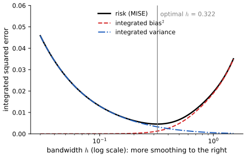
fig_20_2. Download: PDF · SVG20.2 Histograms
See also the histogram as a maximum likelihood estimate in Bayesian and Probabilistic Machine Learning, Result 2.25.
Definition 20.B (the histogram estimator) pp. 305–306
Let \(X_1,\dots,X_n\) be iid on \([0,1]\) with density \(f\) (any bounded interval can be rescaled to \([0,1]\)). For an integer \(m\) let the bins be
\[B_1=\Big[0,\tfrac1m\Big),\ B_2=\Big[\tfrac1m,\tfrac2m\Big),\ \dots,\ B_m=\Big[\tfrac{m-1}{m},1\Big],\tag{20.7}\]with bin width \(h=1/m\). Let \(\nu_j\) be the number of observations in \(B_j\), \(\hp_j=\nu_j/n\) and \(p_j=\int_{B_j}f(u)\,\d u\). The histogram estimator is
\[\hf_n(x)=\sum_{j=1}^m\frac{\hp_j}{h}\,I(x\in B_j).\tag{20.8}\](The book's upper limit \(n\) is a misprint for \(m\), in the author's errata.) For \(x\in B_j\) and small \(h\), \[\E\hf_n(x)=p_j/h=\frac1h\int_{B_j}f\approx f(x)h/h=f(x).\]
Example 20.2 p. 306 The astronomy data are \(n=1266\) redshifts of galaxies in a "pencil beam" sky survey, a proxy for their distance (they are the 1266 values below 0.2 in the third column of redshift.dat on the book's website). Figure 20.3 shows three histograms on \([0,0.2]\). Too few bins hide the clusters of galaxies (large bias); too many make every bin noisy (large variance).
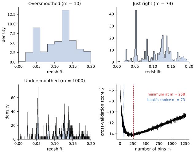
fig_20_3. Download: PDF · SVGTheorem 20.3 (mean and variance of a histogram) p. 306
For fixed \(x\) and \(m\), with \(B_j\) the bin containing \(x\),
\[\E\big(\hf_n(x)\big)=\frac{p_j}{h},\qquad \V\big(\hf_n(x)\big)=\frac{p_j(1-p_j)}{nh^2}.\tag{20.9}\]Proof (Exercise 20.5)
\(\nu_j=\sum_i I(X_i\in B_j)\) is a sum of \(n\) independent Bernoulli\((p_j)\) variables, so \(\nu_j\sim\) Binomial\((n,p_j)\), with mean \(np_j\) and variance \(np_j(1-p_j)\). Since \(\hf_n(x)=\nu_j/(nh)\), its mean is \(p_j/h\) and its variance \(np_j(1-p_j)/(nh)^2\). ∎
Filling the gap 20.2: the histogram is consistent when \(h\to0\) and \(nh\to\infty\) p. 306
If \(f\) is continuous at \(x\), \(h=h_n\to0\) and \(nh_n\to\infty\), then \(\hf_n(x)\toP f(x)\).
Proof
The bin \(B_j\ni x\) has length \(h\) and \[|p_j/h-f(x)|\le\sup_{|u-x|\le h}|f(u)-f(x)|\to0\] by continuity: the bias vanishes. By (20.9), \(\V\hf_n(x)\le p_j/(nh^2)=(p_j/h)/(nh)\), where \(p_j/h\to f(x)\) is bounded and \(nh\to\infty\): the variance vanishes. The mean squared error is bias\(^2\) plus variance, so \(\hf_n(x)\to f(x)\) in mean square, hence in probability (Chebyshev). The two conditions say: the bins shrink, but slowly enough that each holds many points (\(\E\nu_j=np_j\approx nhf(x)\to\infty\)). ∎
Theorem 20.4 (risk of a histogram, the optimal bin width and the \(n^{-2/3}\) rate) pp. 308–309
Suppose \(\int(f'(u))^2\,\d u<\infty\). Then
\[R(\hf_n,f)\approx\frac{h^2}{12}\int(f'(u))^2\,\d u+\frac{1}{nh}.\tag{20.10}\]The value \(h^*\) that minimises (20.10) is
\[h^*=\frac{1}{n^{1/3}}\left(\frac{6}{\int(f'(u))^2\,\d u}\right)^{1/3},\tag{20.11}\]and with this bin width
\[R(\hf_n,f)\approx\frac{C}{n^{2/3}},\qquad C=\Big(\frac34\Big)^{2/3}\Big(\int(f'(u))^2\,\d u\Big)^{1/3}.\tag{20.12}\]Parametric estimators typically have risk of order \(n^{-1}\); the slower \(n^{-2/3}\) is the price of making no parametric assumption.
Filling the gap 20.3: the exact risk of a histogram, and a rigorous version of Theorem 20.4 pp. 308–309
Exact risk. For any density \(f\) on \([0,1]\) (with \(R(f)<\infty\)) and any \(m\), with \(h=1/m\),
\[R(\hf_n,f)=\underbrace{\int f^2-\frac1h\sum_{j=1}^m p_j^2}_{\int b^2}\;+\;\underbrace{\frac{1-\sum_j p_j^2}{nh}}_{\int v}.\]Asymptotics. If moreover \(f'\) is continuous on \([0,1]\), then as \(h\to0\) and \(nh\to\infty\),
\[\int b^2=\frac{h^2}{12}\big(R(f')+o(1)\big),\qquad \int v=\frac{1}{nh}\big(1+o(1)\big).\]Minimising \(ah^2+1/(nh)\) with \(a=R(f')/12\) gives \(2ah^3=1/n\), i.e. (20.11), and at \(h^*\) the bias term is half the variance term, so the risk is \[\tfrac32\cdot\frac{1}{nh^*}=\tfrac32\,6^{-1/3}R(f')^{1/3}n^{-2/3},\] which equals (20.12) because \[\tfrac32\,6^{-1/3}=3^{2/3}2^{-4/3}=(3/4)^{2/3}.\] The same formulas hold for a density on \(\R\) with bins of width \(h\) covering the line (sums over all bins).
Proof
Exact risk. On \(B_j\) the bias is \(p_j/h-f(x)\), so \[\int_{B_j}b^2=\int_{B_j}f^2-2\frac{p_j}{h}p_j+\frac{p_j^2}{h^2}h=\int_{B_j}f^2-\frac{p_j^2}{h};\] sum over \(j\). By (20.9), \[\int v=\sum_j h\cdot\frac{p_j(1-p_j)}{nh^2}=\frac{1-\sum_jp_j^2}{nh}\] since \(\sum_jp_j=1\).
Variance term. \(\sum_jp_j^2\le\max_jp_j\le h\sup f\to0\), so \(\int v=(1+o(1))/(nh)\).
Bias term. Let \(c_j\) be the centre of \(B_j\) and \(\omega(h)=\sup_{|s-t|\le h}|f'(s)-f'(t)|\), which tends to 0 because \(f'\) is uniformly continuous on \([0,1]\). By Taylor's theorem with integral remainder, \(f(u)=f(c_j)+f'(c_j)(u-c_j)+\rho(u)\) with \(|\rho(u)|\le\omega(h)|u-c_j|\le\omega(h)h/2\) on \(B_j\). Averaging over \(B_j\) kills the linear term (\(c_j\) is the centre): \(p_j/h=f(c_j)+\bar\rho_j\) with \(|\bar\rho_j|\le\omega(h)h/2\). Hence, on \(B_j\),
\[b(x)=-f'(c_j)(x-c_j)+e(x),\qquad |e(x)|\le\omega(h)h .\]Since \(\int_{B_j}(x-c_j)^2\d x=h^3/12\) and, by Cauchy-Schwarz, the cross term is at most \[2|f'(c_j)|\,\omega(h)h\cdot\int_{B_j}|x-c_j|\,\d x\le|f'(c_j)|\omega(h)h^3/2,\]
\[\int_0^1b^2=\frac{h^2}{12}\sum_j h\,f'(c_j)^2+O\Big(h^2\omega(h)\sum_jh|f'(c_j)|\Big)+O\big(h^2\omega(h)^2\big).\]\(\sum_jhf'(c_j)^2\) is a Riemann sum for \(R(f')\) and \(\sum_jh|f'(c_j)|\) one for \(\int|f'|\); both converge, and \(\omega(h)\to0\). So \(\int b^2=\frac{h^2}{12}(R(f')+o(1))\). ∎
The exact formula is what the rates demo and Figure 20.S1 use; it confirms numerically that \(h^*\) of (20.11) and the exact minimiser differ by less than 0.5% at \(n=10^6\), and that (20.12) is then within 1% of the exact optimal risk.
pp. 309–310 The optimal \(h^*\) depends on the unknown \(f\). A practical choice estimates the risk. The loss is \(L(h)=\int\hf_n^2-2\int\hf_nf+\int f^2\); the last term does not depend on \(h\), so minimising the risk is the same as minimising \(\E J(h)\), where \(J(h)=\int\hf_n^2-2\int\hf_nf\).
Definition 20.5 (cross-validation estimator of risk) p. 310
\[\hJ(h)=\int\big(\hf_n(x)\big)^2\d x-\frac2n\sum_{i=1}^n\hf_{(-i)}(X_i),\tag{20.13}\]where \(\hf_{(-i)}\) is the histogram computed without the \(i\)th observation. \(\hJ(h)\) is the cross-validation score or estimated risk.
Theorem 20.6 (the score is unbiased) p. 310
The book states \(\E\hJ(h)\approx\E J(h)\). In fact the equality is exact: \(\E\hJ(h)=\E J(h)\) for every \(h\) and \(n\ge2\) (Filling the gap 20.4).
Theorem 20.7 (the shortcut) p. 310
As corrected in the author's errata,
\[\hJ(h)=\frac{2}{(n-1)h}-\frac{n+1}{(n-1)h}\sum_{j=1}^m\hp_j^{\,2}.\tag{20.14}\]One histogram per \(m\) is enough; the whole curve of Figure 20.3 for \(m=1,\dots,1266\) takes a fraction of a second.
Filling the gap 20.4: why the score is exactly unbiased, and the proof of (20.14) p. 310
Proofs (Exercise 20.6)
Shortcut. \[\int\hf_n^2=\sum_j(\hp_j/h)^2h=\sum_j\hp_j^2/h.\] If \(X_i\in B_j\), removing it leaves \(\nu_j-1\) of the other \(n-1\) points in \(B_j\), so \(\hf_{(-i)}(X_i)=(\nu_j-1)/((n-1)h)\). Summing over the \(\nu_j\) points of each bin,
\[\sum_{i=1}^n\hf_{(-i)}(X_i)=\sum_j\frac{\nu_j(\nu_j-1)}{(n-1)h}=\frac{n^2\sum_j\hp_j^2-n}{(n-1)h}.\]Therefore \[\hJ(h)=\frac{\sum_j\hp_j^2}{h}-\frac{2n\sum_j\hp_j^2-2}{(n-1)h}=\frac{2}{(n-1)h}-\frac{n+1}{(n-1)h}\sum_j\hp_j^2,\] using \(1-\frac{2n}{n-1}=-\frac{n+1}{n-1}\).
Exact unbiasedness. By symmetry \[\E\frac1n\sum_i\hf_{(-i)}(X_i)=\E\hf_{(-1)}(X_1).\] Given \(X_1=x\), \(\hf_{(-1)}(x)\) is a histogram of the \(n-1\) independent points \(X_2,\dots,X_n\), whose mean is \(p_{j(x)}/h\) by (20.9): the same mean as \(\hf_n(x)\), because a histogram's expectation does not depend on the sample size. Hence
\[\E\hf_{(-1)}(X_1)=\int\frac{p_{j(x)}}{h}f(x)\,\d x=\sum_j\frac{p_j^2}{h}=\int\E\hf_n(x)f(x)\,\d x=\E\int\hf_nf,\]so \(\E\hJ(h)=\E J(h)\). With (20.9) both equal \[\frac{1}{nh}-\big(1+\frac1n\big)\frac1h\sum_jp_j^2:\] the exact risk of Filling the gap 20.3 minus \(\int f^2\). ∎
The book's printed (20.14) lacks the factor \(h\) in the second denominator; with it, the score on the redshifts would be off by more than 1 (e.g. at \(m=73\)). The corrected formula agrees with brute-force leave-one-out to rounding error on both the galaxy and the glass data, and the average of 3000 simulated scores matches the exact expectation \(-0.22297\) (for \(n=300\), \(m=25\), the bimodal mixture).
Example 20.8 p. 310 The cross-validation curve for the redshifts is flat near its minimum (Figure 20.3, bottom right). The book reports that any \(m\) from 73 to 310 is nearly optimal and uses \(m=73\). On the data as distributed on the book's website, the score is smallest at \(m=258\) and within 3% of its minimum for \(m\) from 80 to 335; \(m=73\) is 7% above the minimum. The histogram changes little over that range.
pp. 310–311 Confidence statements about the fine detail of \(f\) are not realistic; the book makes them at the resolution of the histogram, for the "histogramised" density
\[\bfn(x)=\E\big(\hf_n(x)\big)=\frac{p_j}{h}\quad\text{for }x\in B_j.\tag{20.15}\]Definition 20.9 (confidence band) p. 311
A pair of functions \((\ell_n(x),u_n(x))\) is a \(1-\alpha\) confidence band (or envelope) for \(\bfn\) if
\[\P\big(\ell_n(x)\le\bfn(x)\le u_n(x)\ \text{for all }x\big)\ge1-\alpha.\tag{20.16}\]Theorem 20.10 (a confidence envelope for the histogram) p. 311
Let \(m=m(n)\to\infty\) with \(m(n)\log n/n\to0\). Define
\[\ell_n(x)=\Big(\max\big\{\sqrt{\hf_n(x)}-c,\,0\big\}\Big)^2,\qquad u_n(x)=\Big(\sqrt{\hf_n(x)}+c\Big)^2,\tag{20.17}\] \[c=\frac{z_{\alpha/(2m)}}{2}\sqrt{\frac mn}.\tag{20.18}\]Then \((\ell_n,u_n)\) is an approximate \(1-\alpha\) confidence band for \(\bfn\). For data on an interval of length \(L\) instead of \([0,1]\), \(c=z_{\alpha/(2m)}/(2\sqrt{nh})\) with \(h=L/m\), the same formula.
Filling the gap 20.5: the square root, the union bound, and the conditions p. 311
The proof outline of the book has three steps; here is what each needs.
- Why the square root. \(\hp_j\) is approximately \(\N(p_j,p_j(1-p_j)/n)\); its standard deviation depends on the unknown \(p_j\). With \(g(p)=\sqrt p\), the delta method (Theorem 5.13) gives \[2\sqrt n(\sqrt{\hp_j}-\sqrt{p_j})\approx\N(0,1-p_j)\approx\N(0,1)\] when \(p_j\) is small: a variance-stabilising transformation, so one constant \(c\) serves every bin.
- Independence is not needed. The event that the band fails is \[\bigcup_j\{2\sqrt n|\sqrt{\hp_j}-\sqrt{p_j}|>z_{\alpha/(2m)}\},\] and the union bound (Bonferroni) gives probability at most \(\sum_j\P(\cdot)\approx m\cdot\alpha/m=\alpha\) whatever the dependence. (The multinomial correlations, \[-\sqrt{p_jp_k}/\sqrt{(1-p_j)(1-p_k)}\approx-1/m,\] are small; this only says that the bound is not very conservative.)
- The tails must be Normal. The approximation \(\P(|Z_j|>z_{\alpha/(2m)})\approx\alpha/m\) is used at a level \(z_{\alpha/(2m)}\approx\sqrt{2\log m}\) that grows with \(m\): a moderate-deviation statement, not the central limit theorem. By Cramér's moderate-deviation theorem it holds uniformly in \(j\) when each bin's expected count \(np_j\) grows faster than \((\log m)^3\). If \(f\) is bounded below on \([0,1]\), \(np_j\ge cn/m\), and a sufficient condition is \(m(\log n)^3/n\to0\), slightly stronger than the book's \(m\log n/n\to0\). Bins with only a few expected points (in the tails of a density) can break the band.
The delta-method step in detail
\(\sqrt n(\hp_j-p_j)\leadsto\N(0,p_j(1-p_j))\) by the central limit theorem, and \(g'(p)=1/(2\sqrt p)\), so \[\sqrt n(\sqrt{\hp_j}-\sqrt{p_j})\leadsto\N\big(0,p_j(1-p_j)/(4p_j)\big)=\N(0,(1-p_j)/4).\] Then \[|\sqrt{\hf_n(x)}-\sqrt{\bfn(x)}|=|\sqrt{\hp_j}-\sqrt{p_j}|/\sqrt h\] for \(x\in B_j\), so \(\max_x|\sqrt{\hf_n}-\sqrt{\bfn}|\le c\) is the event \[\max_j2\sqrt n|\sqrt{\hp_j}-\sqrt{p_j}|\le 2c\sqrt{nh}=z_{\alpha/(2m)},\] and \[\{\sqrt{\bfn}\in[\sqrt{\hf_n}-c,\sqrt{\hf_n}+c]\}\] is exactly \(\{\ell_n\le\bfn\le u_n\}\) (squaring is increasing on \([0,\infty)\), and \(\sqrt{\bfn}\ge0\) explains the \(\max\{\cdot,0\}\)). In a simulation (bimodal mixture on \((-3,3)\), \(m\) near its optimum, \(n=250\) to \(4000\)) the envelope covered \(\bfn\) on \([-2.5,2.5]\) in 97 to 98% of samples: conservative, as the union bound predicts (Figure 20.S4(a)). ∎
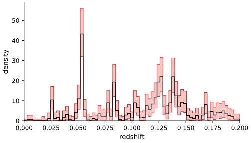
fig_20_4. Download: PDF · SVG20.3 Kernel Density Estimation
See also Statistical Learning, Section 6.6.1, Statistical Methods for Modern Biology, Section 3.6.4, and Bayesian and Probabilistic Machine Learning, Section 2.5.1.
p. 312 Histograms are discontinuous; kernel estimators are smooth and converge faster. In this chapter a kernel is a smooth function with \(K(x)\ge0\), \(\int K=1\), \(\int xK(x)\,\d x=0\) and \(\sigma_K^2=\int x^2K(x)\,\d x>0\). Two examples are the Epanechnikov kernel
\[K(x)=\begin{cases}\frac34\big(1-x^2/5\big)/\sqrt5, & |x|<\sqrt5,\\ 0 & \text{otherwise,}\end{cases}\tag{20.20}\]scaled so that \(\sigma_K^2=1\), and the Gaussian kernel \(K(x)=(2\pi)^{-1/2}e^{-x^2/2}\).
Definition 20.12 (kernel density estimator) p. 313
Given a kernel \(K\) and a bandwidth \(h>0\),
\[\hf_n(x)=\frac1n\sum_{i=1}^n\frac1hK\Big(\frac{x-X_i}{h}\Big).\tag{20.21}\]Each observation contributes a lump of mass \(1/n\) of width proportional to \(h\). As \(h\to0\) the estimate becomes spikes at the data, with heights tending to infinity; as \(h\to\infty\) it flattens out.
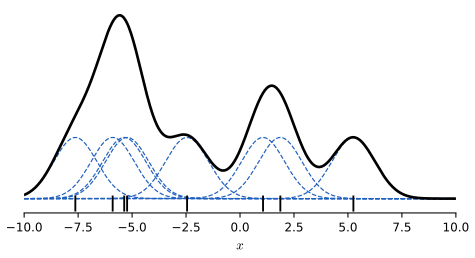
fig_20_5. Download: PDF · SVGExample 20.13 p. 314 Figure 20.6 shows Gaussian kernel estimates of the redshift density with three bandwidths. The cross-validated one shows the same clusters as the histogram, more legibly.
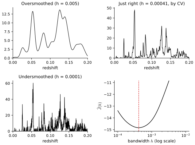
fig_20_6. Download: PDF · SVGFilling the gap 20.6: the choice of kernel matters little, and the Epanechnikov kernel is optimal p. 314, footnote 2
By (20.22) below, the risk at the optimal bandwidth is \[\frac54\big(\sigma_K\int K^2\big)^{4/5}R(f'')^{1/5}n^{-4/5}\] (see Filling the gap 20.7); the kernel enters only through \(\sigma_K\int K^2\), which does not change when \(K\) is rescaled (\(K\mapsto K(\cdot/s)/s\) multiplies \(\sigma_K\) by \(s\) and \(\int K^2\) by \(1/s\)). So we may fix \(\sigma_K=1\) and ask which kernel minimises \(\int K^2\).
Claim. Among non-negative \(K\) with \(\int K=1\), \(\int xK=0\) and \(\int x^2K=1\), the Epanechnikov kernel \(K_E\) of (20.20) minimises \(\int K^2\), with \(\int K_E^2=3/(5\sqrt5)\). The Gaussian kernel's efficiency, \(\big(\int K_E^2/\int K_G^2\big)^{5/4}\), is 0.951: with a Gaussian kernel about 5% more data give the same risk. Neither the uniform (0.930) nor the triangular kernel (0.986) loses much.
Proof
Write \(K_E(x)=a(1-x^2/5)_+\) with \(a=3/(4\sqrt5)\). Since \(\int(K-K_E)^2\ge0\), \(\int K^2\ge2\int KK_E-\int K_E^2\), so it suffices to show \(\int K_E(K-K_E)\ge0\). On \(|x|<\sqrt5\), \(K_E=a(1-x^2/5)\); outside, \(K_E=0\ge a(1-x^2/5)\) while \(K-K_E=K\ge0\). Hence \(K_E(K-K_E)\ge a(1-x^2/5)(K-K_E)\) everywhere, and
\[\int K_E(K-K_E)\ge a\Big[\int(K-K_E)-\tfrac15\int x^2(K-K_E)\Big]=a\big[(1-1)-\tfrac15(1-1)\big]=0.\]Equality forces \(\int(K-K_E)^2=0\). For the Gaussian kernel \(\int K_G^2=1/(2\sqrt\pi)\), and \[\big(\tfrac{3/(5\sqrt5)}{1/(2\sqrt\pi)}\big)^{5/4}=0.951.\] ∎
The bandwidth, by contrast, changes the risk by orders of magnitude (Figure 20.2).
Theorem 20.14 (risk of the kernel estimator and the \(n^{-4/5}\) rate) pp. 314–316
Under weak assumptions on \(f\) and \(K\),
\[R(f,\hf_n)\approx\frac14\sigma_K^4h^4\int(f''(x))^2\,\d x+\frac{\int K^2(x)\,\d x}{nh}.\tag{20.22}\]The optimal bandwidth is
\[h^*=\frac{c_1^{-2/5}c_2^{1/5}c_3^{-1/5}}{n^{1/5}},\qquad c_1=\int x^2K,\ c_2=\int K^2,\ c_3=\int(f'')^2,\tag{20.23}\]and with it \(R(f,\hf_n)\approx c_4/n^{4/5}\) for a constant \(c_4>0\). Under weak assumptions no nonparametric estimator converges faster than \(n^{-4/5}\).
Filling the gap 20.7: a rigorous proof of Theorem 20.14, the exact variance, and \(c_4\) pp. 314–316
Assumptions. \(K\) is a symmetric probability density with \(\sigma_K^2<\infty\) and \(\int K^2<\infty\); \(f\) is bounded, with \(f''\) continuous and square integrable. Then, as \(h\to0\) and \(nh\to\infty\),
\[\int b^2=\frac{h^4}{4}\sigma_K^4\big(R(f'')+o(1)\big),\qquad \int v=\frac{\int K^2}{nh}-\frac{\int(K_h*f)^2}{n}=\frac{\int K^2}{nh}\big(1+O(h)\big).\]The variance formula is exact, not asymptotic. Minimising \(\frac14c_1^2c_3h^4+c_2/(nh)\) gives \(c_1^2c_3h^5=c_2/n\), which is (20.23); at \(h^*\) the bias term is a quarter of the variance term, so
\[R\approx\frac54\,\frac{c_2}{nh^*}=\frac54\,c_1^{2/5}c_2^{4/5}c_3^{1/5}\,n^{-4/5},\qquad c_4=\tfrac54\,(\sigma_K\textstyle\int K^2)^{4/5}R(f'')^{1/5}.\]For the Gaussian kernel and \(f=\N(0,1)\), \(c_3=3/(8\sqrt\pi)\) and \(h^*=(4/3)^{1/5}n^{-1/5}=1.06\,n^{-1/5}\), the "normal reference rule". (The book's proof sketch contains a Taylor expansion with missing powers of \(hu\), listed in the author's errata.)
Proof
Bias. \[\E\hf_n(x)=\int K_h(x-t)f(t)\,\d t=\int K(u)f(x-hu)\,\d u.\] Taylor's theorem with integral remainder gives \[f(x-hu)=f(x)-huf'(x)+h^2u^2\int_0^1(1-t)f''(x-thu)\,\d t.\] The constant term integrates to \(f(x)\) and the linear term to 0 (\(\int uK=0\)), so
\[\frac{b(x)}{h^2}=\int\!\!\int_0^1u^2K(u)(1-t)\,f''(x-thu)\,\d t\,\d u .\]Replacing \(f''(x-thu)\) by \(f''(x)\) gives \(\frac12\sigma_K^2f''(x)\), since \(\int_0^1(1-t)\d t=\frac12\). By Minkowski's integral inequality, in \(L^2(\d x)\),
\[\Big\|\frac{b}{h^2}-\frac{\sigma_K^2}{2}f''\Big\|_2\le\int\!\!\int_0^1u^2K(u)(1-t)\,\big\|f''(\cdot-thu)-f''\big\|_2\,\d t\,\d u\ \longrightarrow\ 0,\]because translation is continuous in \(L^2\) (\(\|f''(\cdot-s)-f''\|_2\to0\) as \(s\to0\)) and the integrand is dominated by \(2\|f''\|_2u^2K(u)\), which is integrable: dominated convergence. So \[\|b\|_2^2=\frac{h^4}{4}\sigma_K^4(R(f'')+o(1)).\]
Variance. \(\hf_n(x)\) is an average of the iid \(K_h(x-X_i)\), so \[v(x)=\frac1n\big(\E K_h(x-X)^2-(\E K_h(x-X))^2\big).\] By Fubini, \[\int\E K_h(x-X)^2\,\d x=\E\int K_h(x-X)^2\,\d x=\int K_h^2=\frac1h\int K^2,\] and \[\int(\E K_h(x-X))^2\d x=\int(K_h*f)^2\le\int f^2\le\sup f\] (Young's inequality). This is the exact formula. ∎
For a Normal mixture \(f=\sum_kw_k\N(\mu_k,s_k^2)\) and the Gaussian kernel every term is explicit, because convolutions of Normal densities are Normal: \[\int(K_h*f)^2=\sum_{k,l}w_kw_l\phi_{\sqrt{s_k^2+s_l^2+2h^2}}(\mu_k-\mu_l),\] and similarly \(\int(K_h*f)f\) and \(\int f^2\) with \(h^2\) and 0 in place of \(2h^2\) (Marron and Wand, 1992). This exact MISE is behind Figures 20.2 and 20.S1 and the rates demo. The same expansion with pointwise statements is in Statistical Methods for Modern Biology, Result 3.2, and the AMISE bandwidth in Statistical Learning, Result 6.12.
Filling the gap 20.8: consistency under minimal conditions pp. 314–316
Theorem 20.14 needs two derivatives. Consistency needs none: if \(K\) is a bounded density, \(f\) is continuous at \(x\), \(h\to0\) and \(nh\to\infty\), then \(\hf_n(x)\toP f(x)\). Indeed \(b(x)=\int K(u)(f(x-hu)-f(x))\,\d u\to0\) by dominated convergence when \(f\) is bounded (and with a little more care in general), and \[v(x)\le\frac1n\E K_h(x-X)^2\le\frac{\sup K}{nh}\E K_h(x-X),\] where \(\E K_h(x-X)\to f(x)\). Exercise 20.1 is the special case of the boxcar kernel. Smoothness assumptions are what turn "consistent" into "consistent at a rate".
Filling the gap 20.9: no estimator converges faster than \(n^{-4/5}\) p. 316
Let \(\mathcal F\) be the densities on \(\R\) with \(|f''|\le L\). The book's claim is a minimax lower bound (Section 12.4). The pointwise version has a short complete proof by Le Cam's two-point method: there is \(c>0\) such that for every estimator \(T_n\) of \(f(x_0)\),
\[\sup_{f\in\mathcal F}\E_f\big(T_n-f(x_0)\big)^2\ \ge\ c\,n^{-4/5}.\]The integrated version, \(\inf_{\hf}\sup_{f}R(f,\hf)\ge c'n^{-4/5}\), follows from the same construction with about \(1/h\) disjoint bumps and Assouad's lemma (Tsybakov, 2009, Chapter 2). Since the kernel estimator attains \(n^{-4/5}\), the rate is optimal.
Proof of the pointwise bound
Two hypotheses. Fix \(f_0\in\mathcal F\) with \(|f_0''|\le L/2\) and \(f_0\ge\gamma>0\) on \([x_0-1,x_0+1]\) (a wide Normal density will do). Let \(\psi(u)=(1-u^2)^3(1-9u^2)\) on \([-1,1]\) and 0 outside: it is twice continuously differentiable, \(\int\psi=0\) and \(\psi(0)=1\). For \(h\le1\) put \(f_1(x)=f_0(x)+ah^2\psi((x-x_0)/h)\) with \(a=L/(2\sup|\psi''|)\). Then \(\int f_1=1\), \(|f_1''|\le L/2+a\sup|\psi''|=L\), and \(f_1\ge0\) once \(ah^2\sup|\psi|\le\gamma\). Both are in \(\mathcal F\), and \(f_1(x_0)-f_0(x_0)=ah^2\).
They are hard to tell apart. With \(P_i\) the law of the sample under \(f_i\), \[\KL(P_1\|P_0)=n\KL(f_1\|f_0)\le n\int\frac{(f_1-f_0)^2}{f_0}\le\frac{n}{\gamma}a^2h^4\cdot h\int\psi^2=\frac{a^2\int\psi^2}{\gamma}\,nh^5.\] Choose \(h=n^{-1/5}\): the divergence is bounded by a constant \(\kappa\).
Le Cam. For any \(T\), \[(T-\theta_0)^2+(T-\theta_1)^2\ge(\theta_1-\theta_0)^2/2,\] so with \(p_0,p_1\) the sample densities,
\[\max_i\E_i(T-\theta_i)^2\ge\tfrac12\big[\E_0(T-\theta_0)^2+\E_1(T-\theta_1)^2\big]\ge\tfrac12\int\min(p_0,p_1)\,\frac{(\theta_1-\theta_0)^2}{2}\ge\frac{a^2h^4}{8}\cdot\frac{e^{-\kappa}}{2},\]using the Bretagnolle-Huber inequality \(\int\min(p_0,p_1)\ge\frac12e^{-\KL(P_1\|P_0)}\). With \(h=n^{-1/5}\) the right side is a constant times \(n^{-4/5}\). ∎
The same argument with \(|f'|\le L\) and a bump of height \(h\) gives \(n^{-2/3}\): the histogram's rate is optimal for that class, and it cannot exploit a second derivative, because its bias is first order in \(h\) (Filling the gap 20.3).
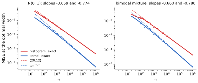
fig_20_S1. Download: PDF · SVGp. 316 Like (20.11), the optimal bandwidth depends on the unknown \(f\). The risk (up to a constant) is estimated by the cross-validation score
\[\hJ(h)=\int\hf^2(x)\,\d x-\frac2n\sum_{i=1}^n\hf_{-i}(X_i),\tag{20.24}\]where \(\hf_{-i}\) is the estimator without the \(i\)th observation.
Theorem 20.15 (unbiasedness and a formula for the score) p. 316
For every \(h>0\), \(\E\hJ(h)=\E J(h)\). Also
\[\hJ(h)\approx\frac{1}{hn^2}\sum_i\sum_jK^*\Big(\frac{X_i-X_j}{h}\Big)+\frac{2}{nh}K(0),\tag{20.25}\]with \(K^*(x)=K^{(2)}(x)-2K(x)\) and \(K^{(2)}(z)=\int K(z-y)K(y)\,\d y\). For the \(\N(0,1)\) kernel, \(K^{(2)}\) is the \(\N(0,2)\) density.
Filling the gap 20.10: proof of Theorem 20.15, and the exact formula behind (20.25) p. 316
Proof (Exercise 20.7)
Unbiasedness. As for the histogram (Filling the gap 20.4): \(\E\hf_m(x)=(K_h*f)(x)\) does not depend on the sample size \(m\), and \(\hf_{-1}\) is independent of \(X_1\), so \[\E\frac1n\sum_i\hf_{-i}(X_i)=\E\hf_{-1}(X_1)=\int(K_h*f)f=\E\int\hf_nf.\] Hence \(\E\hJ=\E\int\hf_n^2-2\E\int\hf_nf=\E J\), exactly.
The exact formula. \[\int\hf_n^2=\frac{1}{n^2}\sum_{i,j}\int K_h(x-X_i)K_h(x-X_j)\,\d x=\frac{1}{n^2h}\sum_{i,j}K^{(2)}\big(\frac{X_i-X_j}{h}\big)\] (substitute \(x=X_j+hy\)), and \[\hf_{-i}(X_i)=\frac{1}{(n-1)h}\sum_{j\ne i}K\big(\frac{X_i-X_j}{h}\big).\] So
\[\hJ(h)=\frac{1}{n^2h}\sum_{i,j}K^{(2)}\Big(\frac{X_i-X_j}{h}\Big)-\frac{2}{n(n-1)h}\sum_{i\ne j}K\Big(\frac{X_i-X_j}{h}\Big).\]Replacing \(n-1\) by \(n\) and writing \(\sum_{i\ne j}=\sum_{i,j}-nK(0)\) gives (20.25); the error is \(\frac{1}{n}\) times the second term, of relative order \(1/n\). For Normal kernels, \(K^{(2)}\) is the density of the sum of two independent \(\N(0,1)\) variables. The code computes the exact formula from the \(n(n-1)/2\) pairwise differences, which it checks against brute-force leave-one-out. Least-squares cross-validation is also Statistical Learning, Result 6.13 (Rudemo, 1982; Bowman, 1984). ∎
Figure 20.S3(b) shows the exact \(\E J(h)\) (computed as in Filling the gap 20.7) and the average of 200 simulated scores on top of each other, with single scores scattered around them.
Theorem 20.16 (Stone's theorem) p. 316
Suppose \(f\) is bounded. Let \(\hf_h\) be the kernel estimator with bandwidth \(h\) and \(\hat h_n\) the bandwidth chosen by cross-validation. Then
\[\frac{\int\big(f(x)-\hf_{\hat h_n}(x)\big)^2\d x}{\inf_h\int\big(f(x)-\hf_h(x)\big)^2\d x}\toP1.\tag{20.26}\]Filling the gap 20.11: how Stone's theorem is proved, and when rounding breaks cross-validation pp. 316–317
The reduction. Write \(I(h)=\int(\hf_h-f)^2=J(h)+\int f^2\), let \(h^\circ\) minimise \(I\), and let \[\varepsilon_n=\sup_h|\hJ(h)+\int f^2-I(h)|/I(h)\] over the range of bandwidths considered. Since \(\hJ(\hat h_n)\le\hJ(h^\circ)\),
\[I(\hat h_n)(1-\varepsilon_n)\le\hJ(\hat h_n)+\textstyle\int f^2\le\hJ(h^\circ)+\int f^2\le I(h^\circ)(1+\varepsilon_n),\]so \[1\le I(\hat h_n)/I(h^\circ)\le(1+\varepsilon_n)/(1-\varepsilon_n).\] Stone's theorem is therefore equivalent to \(\varepsilon_n\toP0\): the score's error, after removing the constant \(\int f^2\), is uniformly small relative to the loss itself. Proving this is the hard part (Stone, 1984): \(\hJ(h)+\int f^2-I(h)\) is a degenerate \(U\)-statistic plus a linear term, and exponential inequalities for both, applied on a fine grid of \(h\) and extended by continuity, give the uniform bound. The theorem says nothing about the rate at which the ratio approaches 1; the cross-validated bandwidth itself is very variable, \(\hat h_n/h^\circ-1\) being of order \(n^{-1/10}\) (Hall and Marron, 1987).
Rounding (Example 20.17). Suppose \(T\) ordered pairs \(i\ne j\) have \(X_i=X_j\). As \(h\to0\) every term with \(X_i\ne X_j\) vanishes in the exact formula of Filling the gap 20.10, and
\[h\,\hJ(h)\ \to\ \frac{(n+T)K^{(2)}(0)}{n^2}-\frac{2T\,K(0)}{n(n-1)}.\]For the Gaussian kernel \(K^{(2)}(0)=K(0)/\sqrt2\), so the limit is negative, and \(\hJ(h)\to-\infty\) as \(h\to0\), exactly when \(T\) exceeds about \(n/(2\sqrt2-1)\approx0.55\,n\): when there are enough ties, cross-validation picks \(h\to0\). The redshifts on the book's website have \(T=20\), far below the threshold 692; rounded to three decimals they have \(T=23{,}872\), and the score collapses (Figure 20.S3(a)). Adding small Normal noise (the book's remedy) breaks the ties; the noise level then affects the chosen bandwidth. The same phenomenon is analysed in Statistical Learning, Filling the gap 6.8.
Remark 20.18 p. 317: a wiggly cross-validated estimate is not evidence of failure; the eye is a poor judge of integrated squared error.
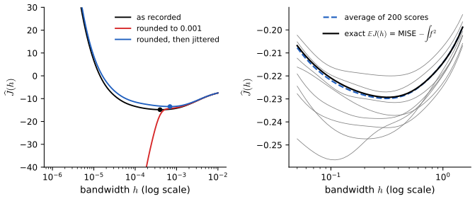
fig_20_S3. Download: PDF · SVGp. 317 As for histograms, the band is for the smoothed density \[\bfn(x)=\E\hf_n(x)=\int\frac1hK\big(\frac{x-u}{h}\big)f(u)\,\d u.\] For a density on \((a,b)\) the band (a modification of Chaudhuri and Marron, 1999) is
\[\ell_n(x)=\hf_n(x)-q\,\se(x),\qquad u_n(x)=\hf_n(x)+q\,\se(x),\tag{20.27}\]where \(\se(x)=s(x)/\sqrt n\), \[s^2(x)=\frac{1}{n-1}\sum_i(Y_i(x)-\bar Y_n(x))^2,\] \(Y_i(x)=\frac1hK\big(\frac{x-X_i}{h}\big)\), \[q=\Phi^{-1}\big(\frac{1+(1-\alpha)^{1/m}}{2}\big),\] \(m=(b-a)/\omega\), and \(\omega\) is the width of the kernel (\(\omega=3h\) for the Normal kernel).
Filling the gap 20.12: where (20.27) comes from, and how well it covers p. 317
\(\hf_n(x)=\bar Y_n(x)\) is an average of iid variables with mean \(\bfn(x)\), so \(\se(x)\) is its usual standard error and \((\hf_n(x)-\bfn(x))/\se(x)\approx\N(0,1)\) at each \(x\) (central limit theorem and Slutsky). Values of \(\hf_n\) at points more than a kernel width \(\omega\) apart depend on nearly disjoint sets of observations and are nearly independent; treating the interval as \(m=(b-a)/\omega\) independent pieces, the probability that all \(m\) standardised errors are below \(q\) in absolute value is \((2\Phi(q)-1)^m\), and setting this to \(1-\alpha\) gives the stated \(q\) (Šidák's correction; it is slightly smaller than the Bonferroni value \(z_{\alpha/(2m)}\)). This is a heuristic: the supremum of the standardised process over a continuum is governed by extreme-value theory (Bickel and Rosenblatt, 1973), and the "number of independent pieces" depends on the kernel's correlation length. In a simulation (Figure 20.S4(a)) the band covered \(\bfn\) on \([-2.5,2.5]\) in 75 to 91% of samples at nominal 95%, so it is somewhat optimistic for these sample sizes. For the redshifts with the cross-validated \(h\), \(m=161\) and \(q=3.60\) (Figure 20.7).
Example 20.19 p. 317 Figure 20.7 shows the 95% band for the redshift density.
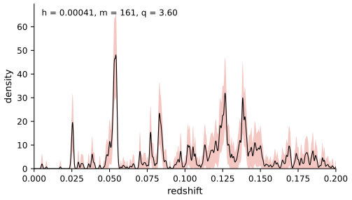
fig_20_7. Download: PDF · SVGp. 318 For \(d\)-dimensional data \(X_i=(X_{i1},\dots,X_{id})\), with bandwidths \(h=(h_1,\dots,h_d)\),
\[\hf_n(x)=\frac1n\sum_{i=1}^nK_h(x-X_i),\tag{20.28}\] \[K_h(x-X_i)=\frac{1}{h_1\cdots h_d}\prod_{j=1}^dK\Big(\frac{x_j-X_{ij}}{h_j}\Big).\tag{20.29}\](The book's (20.29) has an extra factor \(n\) in the denominator, already present in (20.28), and \(x_i\) for \(x_j\); see Notes on the book.) A simple choice is \(h_j=s_jh\), with \(s_j\) the standard deviation of the \(j\)th variable. The risk is
\[R(f,\hf_n)\approx\frac14\sigma_K^4\Big[\sum_{j=1}^dh_j^4\!\int f_{jj}^2(x)\,\d x+\sum_{j\ne k}h_j^2h_k^2\!\int f_{jj}f_{kk}\,\d x\Big]+\frac{\big(\int K^2\big)^d}{nh_1\cdots h_d},\]where \(f_{jj}\) is a second partial derivative. The optimal bandwidths are of order \(n^{-1/(4+d)}\) and the risk of order \(n^{-4/(4+d)}\): the curse of dimensionality.
Filling the gap 20.13: the \(d\)-dimensional risk, its rate, and Silverman's table recomputed pp. 318–319
The risk. The proof of Filling the gap 20.7 goes through coordinate by coordinate. With \(u=(x-t)/h\) componentwise, \[\E\hf_n(x)=\int\prod_jK(u_j)f(x-h\circ u)\,\d u,\] and the second-order Taylor expansion of \(f\) has cross terms \(h_jh_ku_ju_kf_{jk}\) that integrate to 0 for \(j\ne k\) (the \(u_j\) are independent with mean 0 under the product kernel), leaving \[b(x)\approx\frac12\sigma_K^2\sum_jh_j^2f_{jj}(x);\] squaring and integrating gives the bracket. The variance is exactly \[\frac1n\big[\prod_j\frac{\int K^2}{h_j}-\int(K_h*f)^2\big].\]
The rate. With all \(h_j\) proportional to one \(h\), the risk is \(Ah^4+B/(nh^d)\), minimised at \(h\propto n^{-1/(4+d)}\), where it is of order \(n^{-4/(4+d)}\): \(n^{-4/5}\) for \(d=1\), \(n^{-2/3}\) for \(d=2\), \(n^{-2/7}\) for \(d=10\).
Silverman's table. The book quotes from Silverman (1986) the sample size needed for a relative mean squared error at the origin below 0.1, for the \(d\)-dimensional standard Normal density estimated with a Normal kernel and the best bandwidth. Everything is explicit: with \(f=\N(0,I_d)\) and kernel \(\N(0,h^2I_d)\),
\[\E\hf_n(0)=(2\pi(1+h^2))^{-d/2},\qquad \V\hf_n(0)=\frac1n\Big[\Big(\frac{1}{2\sqrt\pi\,h\sqrt{2\pi(1+h^2/2)}}\Big)^d-\big(\E\hf_n(0)\big)^2\Big],\]so the relative MSE \[\big(\V\hf_n(0)+(\E\hf_n(0)-f(0))^2\big)/f(0)^2\] can be minimised over \(h\) and the \(n\) at which the minimum equals 0.1 found by bisection. The result, rounded up: 4, 19, 67, 223, 768, 2788, 10730, 43684, 187275, 841566 for \(d=1,\dots,10\), which matches every entry of the table (4, 19, 67, 223, 768, 2790, 10,700, 43,700, 187,000, 842,000) to its three significant figures. The same table is discussed in Statistical Learning, Filling the gap 6.5.
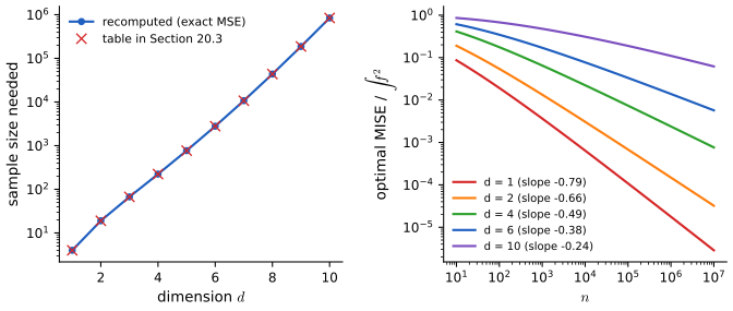
fig_20_S2. Download: PDF · SVG20.4 Nonparametric Regression
See also Statistical Learning, Sections 6.1 and 6.2, and local regression in Applied Statistical Learning, Section 7.6.
p. 319 Consider pairs \((x_1,Y_1),\dots,(x_n,Y_n)\) with
\[Y_i=r(x_i)+\epsilon_i,\qquad\E(\epsilon_i)=0.\tag{20.30}\]The \(x_i\) are treated as fixed (in regression only the conditional mean of \(Y\) given \(x\) matters). Most estimators of \(r(x)=\E(Y\given X=x)\) are weighted averages of the \(Y_i\), with more weight on the points near \(x\).
Definition 20.20 (Nadaraya-Watson kernel estimator) pp. 319–320
\[\hr_n(x)=\sum_{i=1}^nw_i(x)Y_i,\tag{20.31}\] \[w_i(x)=\frac{K\big(\frac{x-x_i}{h}\big)}{\sum_{j=1}^nK\big(\frac{x-x_j}{h}\big)}.\tag{20.32}\]The weights are non-negative and sum to 1. Like every estimator in this section, \(\hr_n\) is a linear smoother: the vector of fitted values is \(LY\) with \(L_{ij}=w_j(x_i)\), and \(\operatorname{tr}L\) is its effective number of degrees of freedom.
Filling the gap 20.14: Nadaraya-Watson from a kernel density estimate, as local least squares, and its local linear refinement p. 320
From the joint density. Estimate \(f(x,y)\) by the product-kernel estimate \[\hf(x,y)=\frac1n\sum_iK_{h}(x-x_i)K_{g}(y-Y_i)\] with any symmetric \(K_g\). Since \(\int K_g(y-Y_i)\,\d y=1\) and \(\int yK_g(y-Y_i)\,\d y=Y_i\),
\[\frac{\int y\,\hf(x,y)\,\d y}{\int\hf(x,y)\,\d y}=\frac{\frac1n\sum_iK_h(x-x_i)Y_i}{\frac1n\sum_iK_h(x-x_i)}=\hr_n(x),\]whatever the \(y\)-bandwidth: the book's motivation, made exact. (Confirmed numerically on the motorcycle data by integrating over \(y\).)
As local least squares. \[\hr_n(x)=\argmin_c\sum_iK\big(\frac{x-x_i}{h}\big)(Y_i-c)^2:\] a weighted average is the weighted least-squares constant. Fitting a weighted least-squares line \(c+\beta(x_i-x)\) instead and keeping \(c\) gives local linear regression, \(\hr_n(x)=\sum_il_i(x)Y_i\) with
\[l_i(x)=\frac{K_i\,(S_2-(x_i-x)S_1)}{\sum_jK_j\,(S_2-(x_j-x)S_1)},\qquad K_i=K\Big(\frac{x_i-x}{h}\Big),\ S_k=\sum_jK_j(x_j-x)^k .\]It reproduces straight lines exactly (\(\sum_il_i(x)=1\), \(\sum_il_i(x)(x_i-x)=0\)), which removes the design bias and the first-order boundary bias of Nadaraya-Watson (Filling the gap 20.15). The equivalent kernels are drawn in Statistical Learning, Definition 6.2.
Theorem 20.21 (risk of the Nadaraya-Watson estimator) p. 320
Suppose \(\V(\epsilon_i)=\sigma^2\) and the design has density \(f\). Then, corrected (see Notes on the book),
\[R(\hr_n,r)\approx\frac{h^4}{4}\Big(\int x^2K(x)\,\d x\Big)^2\int\Big(r''(x)+2r'(x)\frac{f'(x)}{f(x)}\Big)^2\d x+\int\frac{\sigma^2\int K^2(x)\,\d x}{nhf(x)}\,\d x.\tag{20.33}\]The optimal bandwidth decreases like \(n^{-1/5}\), and with it the risk decreases like \(n^{-4/5}\).
Filling the gap 20.15: where (20.33) comes from: the design bias, the boundary, and local linear regression p. 320
Pointwise bias and variance. For a random design with density \(f\) (or a fixed design whose empirical distribution approximates \(f\)), at an interior point with \(f(x)>0\), \(r\) and \(f\) twice continuously differentiable,
\[\E\hr_n(x)-r(x)\approx h^2\sigma_K^2\Big(\frac{r''(x)}{2}+\frac{r'(x)f'(x)}{f(x)}\Big),\qquad\V\hr_n(x)\approx\frac{\sigma^2\int K^2}{nh\,f(x)}.\]Squaring the bias gives \(\frac{h^4}{4}\sigma_K^4(r''+2r'f'/f)^2\); integrating both over \(x\) gives (20.33), whose first factor is therefore \(\sigma_K^4=(\int x^2K)^2\). Minimising \(Ah^4+B/(nh)\) gives \(h\asymp n^{-1/5}\) and risk \(\asymp n^{-4/5}\), as for densities.
Derivation
Write \(\hr_n=\hg/\hf\) with \(\hg(x)=\frac1n\sum_iK_h(x-X_i)Y_i\) and \(\hf(x)=\frac1n\sum_iK_h(x-X_i)\). By Filling the gap 20.7 applied to the functions \(rf\) and \(f\), \[\E\hg(x)=rf+\frac{h^2\sigma_K^2}{2}(rf)''+o(h^2)\] and \(\E\hf(x)=f+\frac{h^2\sigma_K^2}{2}f''+o(h^2)\). Linearising the ratio around \((rf,f)\), \(\hr_n-r\approx(\hg-r\hf)/f\), so the bias is
\[\frac{h^2\sigma_K^2}{2f}\big((rf)''-rf''\big)=\frac{h^2\sigma_K^2}{2f}\big(r''f+2r'f'\big)=h^2\sigma_K^2\Big(\frac{r''}{2}+\frac{r'f'}{f}\Big).\]For the variance, \(\hg-r\hf=\frac1n\sum_iK_h(x-X_i)(Y_i-r(x))\) has variance \[\frac1n\E[K_h(x-X)^2(Y-r(x))^2]\approx\frac{1}{nh}\sigma^2f(x)\int K^2;\] divide by \(f^2\). (A complete proof bounds the remainder of the ratio expansion; see Statistical Learning, Result 6.3, and Fan and Gijbels, 1996.) ∎
The design bias. The term \(r'f'/f\) appears because, where the design density is increasing, there are more points on one side of \(x\) than on the other, and the average leans towards them. At a boundary the imbalance is extreme and the bias of Nadaraya-Watson is of order \(h\), not \(h^2\). Local linear regression fits a line and so is not fooled by an asymmetric neighbourhood: its interior bias is \(h^2\sigma_K^2r''/2\) and its boundary bias is still of order \(h^2\). Figure 20.S5(a) shows both effects computed exactly (\(\E\hr_n=\sum_il_i(x)r(x_i)\) for a linear smoother), on a design with density \(1.5-x\).
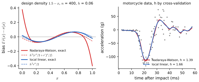
fig_20_S5. Download: PDF · SVGp. 320 The bandwidth is chosen by minimising the cross-validation score
\[\hJ(h)=\sum_{i=1}^n\big(Y_i-\hr_{-i}(x_i)\big)^2,\tag{20.34}\]where \(\hr_{-i}\) is the estimator computed without the \(i\)th pair.
Theorem 20.22 (the score from one fit) p. 320
\[\hJ(h)=\sum_{i=1}^n\big(Y_i-\hr(x_i)\big)^2\frac{1}{\Big(1-\frac{K(0)}{\sum_{j=1}^nK\big(\frac{x_i-x_j}{h}\big)}\Big)^2}.\tag{20.35}\]Filling the gap 20.16: proof of (20.35), and the same identity for local linear regression p. 320
Proof (Exercise 20.10)
Let \(S_i=\sum_jK\big(\frac{x_i-x_j}{h}\big)\) and \(L_{ii}=w_i(x_i)=K(0)/S_i\). Then \[\sum_{j\ne i}K\big(\frac{x_i-x_j}{h}\big)Y_j=S_i\hr(x_i)-K(0)Y_i\] and \[\sum_{j\ne i}K\big(\frac{x_i-x_j}{h}\big)=S_i-K(0),\] so
\[\hr_{-i}(x_i)=\frac{\hr(x_i)-L_{ii}Y_i}{1-L_{ii}},\qquad Y_i-\hr_{-i}(x_i)=\frac{Y_i-\hr(x_i)}{1-L_{ii}}.\]Square and sum. ∎
For local linear regression the fit at \(x_i\) is a weighted least-squares fit, and deleting observation \(i\) from a weighted least-squares fit changes its residual at \(i\) by the factor \(1/(1-H_{ii})\), with \(H_{ii}=l_i(x_i)\): the same formula holds with \(L_{ii}=l_i(x_i)\) (Statistical Learning, Result 6.6; Applied Statistical Learning, Filling the gap 7.8; the least squares case is Filling the gap 13.10). Both identities are confirmed against brute-force refitting in the code. If a point has no neighbours within reach of the kernel, \(L_{ii}=1\) and it cannot be predicted from the others: the score is infinite, which is how the code and the demo treat very small bandwidths.
Example 20.23 pp. 320–321 The book analyses the power spectrum of the cosmic microwave background, as measured by BOOMERaNG, Maxima and DASI: \(x_i\) is the multipole moment and \(Y_i\) the estimated power. Peaks in \(r(x)\) are the signature of sound waves in the early universe. Those measurements are not on the book's website; the WMAP spectrum is, and it is used here, restricted to multipoles \(\ell\le700\) (699 points; beyond that the measurement errors grow rapidly: the quoted standard error reaches 9700 at \(\ell=900\), against at most 2500 below 700). Cross-validation over 121 bandwidths from 2 to 150 picks \(h=23.1\) (12.5 effective degrees of freedom); the fit shows the first peak near \(\ell=220\) and a second near \(\ell=540\).
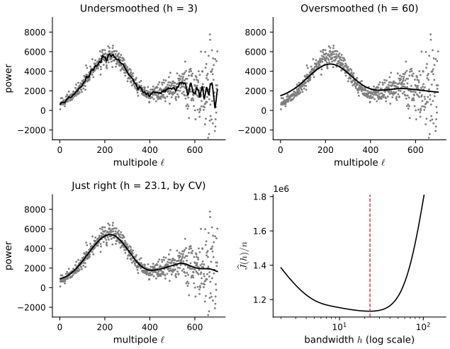
fig_20_8. Download: PDF · SVGp. 321 A confidence band needs an estimate of \(\sigma^2\). With the \(x_i\) ordered and \(r\) smooth, \(Y_{i+1}-Y_i\approx\epsilon_{i+1}-\epsilon_i\), whose variance is \(2\sigma^2\); hence
\[\hs^2=\frac{1}{2(n-1)}\sum_{i=1}^{n-1}(Y_{i+1}-Y_i)^2.\tag{20.36}\]Filling the gap 20.17: the difference estimator is consistent, and how large its bias is p. 321
Suppose the \(\epsilon_i\) are iid with variance \(\sigma^2\) and \(\E\epsilon^4<\infty\), \(r\) is Lipschitz with constant \(L_r\) on \([a,b]\), and the ordered design points satisfy \(\max_i(x_{i+1}-x_i)\to0\). Then \(\hs^2\toP\sigma^2\) (Rice, 1984).
Proof (Exercise 20.9)
Write \(\Delta_i=r(x_{i+1})-r(x_i)\) and \(D_i=\epsilon_{i+1}-\epsilon_i\). Then \((Y_{i+1}-Y_i)^2=\Delta_i^2+2\Delta_iD_i+D_i^2\) and
\[\E\hs^2=\sigma^2+\frac{1}{2(n-1)}\sum_i\Delta_i^2,\qquad\frac{1}{2(n-1)}\sum_i\Delta_i^2\le\frac{L_r^2\max_i(x_{i+1}-x_i)}{2(n-1)}\sum_i(x_{i+1}-x_i)\le\frac{L_r^2(b-a)\max_i(x_{i+1}-x_i)}{2(n-1)}\to0 .\]For the variance: the \(D_i^2\) form a 1-dependent sequence (\(D_i\) and \(D_k\) are independent when \(|i-k|\ge2\)) with \(\V(D_i^2)\le\E D_i^4<\infty\), so \(\V\big(\sum_iD_i^2\big)\le3(n-1)\E D_1^4\); and \[\V\big(\sum_i\Delta_iD_i\big)\le 4\sigma^2\sum_i\Delta_i^2\] by the same 1-dependence. Hence \(\V\hs^2=O(1/n)\). Bias and variance both vanish, so \(\hs^2\to\sigma^2\) in mean square, hence in probability. ∎
For equally spaced designs the bias is \(O(n^{-2})\), negligible; the estimator does not need a bandwidth. Its weakness is the assumption of a constant variance. On the WMAP data \(\hs=1076\); the measurement error is in fact far from constant (Figure 20.9), and on the motorcycle data the noise before the impact is a small fraction of that after it (preset 5 of the regression demo).
pp. 321–323 As for densities, the band is for the smoothed function \(\brn(x)=\E\hr_n(x)\).
Definition 20.C (confidence band for kernel regression) p. 323
An approximate \(1-\alpha\) confidence band for \(\brn(x)\) is
\[\ell_n(x)=\hr_n(x)-q\,\se(x),\qquad u_n(x)=\hr_n(x)+q\,\se(x),\tag{20.37}\]with \(\se(x)=\hs\sqrt{\sum_iw_i^2(x)}\), \[q=\Phi^{-1}\big(\frac{1+(1-\alpha)^{1/m}}{2}\big),\] \(m=(b-a)/\omega\), \(\hs\) from (20.36) and \(\omega\) the width of the kernel (\(\omega=3h\) for the Normal kernel).
Filling the gap 20.18: the standard error of a linear smoother, and what the band assumes p. 323
For any linear smoother \(\hr_n(x)=\sum_iw_i(x)Y_i\) with fixed weights and independent errors of variance \(\sigma^2\), \(\V\hr_n(x)=\sigma^2\sum_iw_i^2(x)\) exactly (variance of a linear combination of independent variables), and \(\E\hr_n(x)=\sum_iw_i(x)r(x_i)=\brn(x)\). If the errors are Normal, \((\hr_n(x)-\brn(x))/(\sigma\|w(x)\|)\) is exactly \(\N(0,1)\); otherwise it is approximately so when many weights are non-negligible (Lindeberg). Replacing \(\sigma\) by the consistent \(\hs\) changes nothing asymptotically (Slutsky). The multiplier \(q\) is the Šidák correction of Filling the gap 20.12. Two assumptions are easy to forget: the errors must have constant variance (a single \(\hs\) multiplies every \(\se(x)\)), and the band is for \(\brn\), not \(r\) (Filling the gap 20.20). In the simulation of Figure 20.S4(c) the band covered \(\brn\) on \([0.1,0.9]\) in 88 to 91% of samples at nominal 95%.
Example 20.24 p. 323 Figure 20.9 shows the 95% band for the spectrum. The position of the first peak is well determined; the second is less certain.
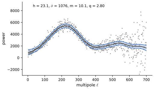
fig_20_9. Download: PDF · SVGpp. 323–324 With several covariates \(X=(X_1,\dots,X_p)\) a multivariate kernel can be used, with the curse of dimensionality of Section 20.3. Restricting the form of \(r\) avoids it. Additive regression assumes
\[Y=\sum_{j=1}^pr_j(X_j)+\epsilon,\tag{20.38}\]so that only \(p\) one-dimensional functions are estimated; it can be enriched with interactions,
\[Y=\sum_{j=1}^pr_j(X_j)+\sum_{j<k}r_{jk}(X_j,X_k)+\epsilon.\tag{20.39}\](The book writes \(r_{jk}(X_jX_k)\), a function of the product, where a function of the pair is meant.)
Algorithm 20.D (backfitting) p. 324
- Initialise \(r_1,\dots,r_p\) (for instance to 0, with the intercept \(\bar Y\)).
- For \(j=1,\dots,p\): form the partial residuals \(\epsilon_i=Y_i-\sum_{s\ne j}r_s(x_{is})\), and let \(r_j\) be the smooth of the \(\epsilon_i\) on the \(j\)th covariate.
- Stop if the functions have converged; otherwise return to step 2.
Filling the gap 20.19: what backfitting solves p. 324
With linear smoothers \(S_j\) (\(n\times n\) matrices) and fitted vectors \(\bm f_j\), a fixed point of backfitting satisfies \(\bm f_j=S_j\big(Y-\sum_{k\ne j}\bm f_k\big)\) for all \(j\): \(p\) blocks of "normal equations", and backfitting is the block Gauss-Seidel method for them. When each \(S_j\) is symmetric with eigenvalues in \([0,1]\) (smoothing splines, for example), these are the stationarity conditions of a penalised least-squares criterion, and Gauss-Seidel converges to a solution (Buja, Hastie and Tibshirani, 1989); for kernel smoothers, which are not symmetric, convergence holds in practice but needs separate arguments. The function backfit in the code recovers \(\sin(2x_1)+x_2^2\) from 300 noisy points with a correlation above 0.98. Additive models avoid the curse of dimensionality, at the price of not being fully nonparametric: the true \(r\) need not be additive. The full proof for symmetric smoothers is Applied Statistical Learning, Result 7.8 with Filling the gap 7.10.
20.5 Appendix
pp. 324–325 Confidence sets and bias. The bands of this chapter are for the smoothed curves \(\bfn\) and \(\brn\), not for \(f\) and \(r\). Writing \(\bar f_n(x)\) and \(s_n(x)\) for the mean and standard deviation of \(\hf_n(x)\),
\[\frac{\hf_n(x)-f(x)}{s_n(x)}=\frac{\hf_n(x)-\bfn(x)}{s_n(x)}+\frac{\bfn(x)-f(x)}{s_n(x)}.\]The first term is approximately standard Normal. The second is bias over standard deviation. In parametric problems it tends to 0; with optimal smoothing it does not, because the optimal bandwidth balances the two.
Filling the gap 20.20: how much the bias costs, exactly, and the cure pp. 324–325
Take a kernel density estimate with \(h=cn^{-1/5}\). By Filling the gap 20.7 the bias is \(\frac12h^2\sigma_K^2f''(x)(1+o(1))\) and the standard deviation \(\sqrt{f(x)\int K^2/(nh)}(1+o(1))\); their ratio tends to the constant
\[\beta(x)=\frac{\tfrac12c^2\sigma_K^2f''(x)}{\sqrt{f(x)\int K^2/c}},\]so the nominal 95% interval \(\hf_n(x)\pm1.96\,\se(x)\) covers \(f(x)\) with probability tending to \(\P(|Z+\beta(x)|\le1.96)<0.95\), however large \(n\) is. At the AMISE-optimal \(c\), the integrated squared bias is a quarter of the integrated variance (Filling the gap 20.7): \(\beta\) is about \(1/2\) "on average", and the coverage about 0.92. At the mode \(x=1\) of the bimodal mixture, \(\beta=-0.668\) and the limiting coverage is 0.898; for the regression function \(\sin(2\pi x)+2x\) with equally spaced design, \(\beta=-1/\sqrt2\) exactly at its peak and the limit 0.891. Figure 20.S4 confirms both by simulation, up to \(n=16{,}000\).
Cures. (i) Undersmoothing: take \(h=o(n^{-1/5})\); then \(\beta(x)\to0\) and the interval is asymptotically exact for \(f(x)\), at the price of a wider interval and a slower rate (the green curves of Figure 20.S4 use \(h=h^*n^{-1/10}\)). (ii) Bias correction: estimate \(f''\) and subtract the leading bias, which in turn requires a second bandwidth. (iii) Accept the book's position: report a band for the smoothed curve and say so.
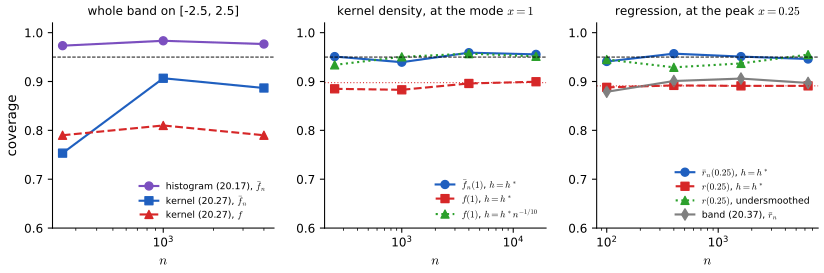
fig_20_S4. Download: PDF · SVG20.6 Bibliographic Remarks
p. 325 Scott (1992) and Silverman (1986) are standard texts on density estimation; Härdle (1990) and Loader (1999) on nonparametric regression, the latter emphasising local likelihood. For the theory of rates and lower bounds see Tsybakov (2009); for local polynomial regression, Fan and Gijbels (1996).
Notes on the book
Twelve slips of Chapter 20 are in the author's errata lists; the other points are mine, each with the evidence.
Page 304, (20.2) and (20.5)
(20.2) should read \(R(g,\hg_n)=\E(L(g,\hg_n))\) and in (20.5) the square belongs outside the bracket. Listed in the author's errata (items 46 and 47 of the first list, item 27 of the second).
Page 306: (20.8), the display before Example 20.2, and "too few bins"
The sum in (20.8) runs to \(m\), not \(n\); the second-last expression of the display should be \(f(x)h/h\); and in Example 20.2 the phrase "and too few bins" should be ignored. Listed in the author's errata (items 48 to 50).
Page 310: (20.14) and "\(\hat A\)"
The second denominator of (20.14) should be \(h(n-1)\), and \(\hat A\) on line −7 should be \(\hJ\). Listed in the author's errata (items 51 and 52). The corrected formula agrees with brute-force leave-one-out (Filling the gap 20.4).
Pages 313–317: "show", the missing \(\d x\), the Taylor expansion, "dz", "which problems"
"show" should be "shown" (p. 313); (20.22) needs a \(\d x\); the bracket in the proof of Theorem 20.14 should read \(f(x)-huf'(x)+\frac{h^2u^2}{2}f''(x)+\cdots\); (20.24) has \(\d x\), not \(\d z\); "which problems" should be "which causes problems" (p. 317). Listed in the author's errata (items 53 to 57).
Page 320, (20.33): the bias constant should be \(\sigma_K^4=(\int x^2K)^2\), not \((\int x^2K^2)^4\)
The bias of the Nadaraya-Watson estimator is \(h^2\sigma_K^2(r''/2+r'f'/f)\) (Filling the gap 20.15), so its square carries \(\sigma_K^4=(\int x^2K(x)\,\d x)^2\), as in (20.22) for densities. The printed \((\int x^2K^2(x)\,\d x)^4\) differs by a large factor (for the Gaussian kernel, \(\int x^2K^2=1/(4\sqrt\pi)\), so the printed factor is \(4.0\times10^{-4}\) instead of 1). The exact bias computed on a fine design matches \(h^2(r''/2+r'f'/f)\) with \(\sigma_K^2=1\) (Figure 20.S5(a)). Not in the errata lists.
Page 318, (20.29): an extra \(n\), and \(x_i\) for \(x_j\)
(20.28) already divides by \(n\); with the printed \(K_h=\frac{1}{nh_1\cdots h_d}\prod_jK(\cdot)\) the estimate would integrate to \(1/n\). The argument of the \(j\)th factor should be \((x_j-X_{ij})/h_j\). Confirmed numerically: the corrected estimator integrates to 1. Not in the errata lists.
Page 310, Theorem 20.6: the score is exactly unbiased, and its argument is \(h\)
The theorem writes \(\E(\hJ(x))\approx\E(J(x))\). The argument is the bin width \(h\), and the equality is exact for every \(n\ge2\) (Filling the gap 20.4); the same is true of the kernel score, as Theorem 20.15 states. Not in the errata lists.
Page 311, proof of Theorem 20.10: \(f\) should be \(\bfn\)
The event \(A\) and the following display compare \(\sqrt{\hf_n}\) with \(\sqrt f\); the band is for \(\bfn\), and the next step (\(\sqrt{p_j/h}\)) uses \(\bfn\). Not in the errata lists.
Examples 20.8, 20.17 and 20.23: the data on the website differ from the book's
On the redshift data as distributed, the histogram score is smallest at \(m=258\), not in the book's 73 to 310 with 73 chosen (the flat range within 3% of the minimum is 80 to 335); only nine values are repeated, so the kernel score does not collapse to \(h=0\) and needs no jitter, and its minimiser is \(h=0.00041\) rather than the \(\approx0.002\) of the book's Figure 20.6 (Filling the gap 20.11). The CMB measurements of Example 20.23 are not on the website; the WMAP spectrum is used instead. These are differences of data, not errors.
Page 323, (20.39): \(r_{jk}(X_jX_k)\) should be \(r_{jk}(X_j,X_k)\)
An interaction term is a function of the pair of covariates; a function of their product is a much smaller class. Not in the errata lists.
20.7 Exercises
All ten exercises of Chapter 20 (Wasserman, 2004, pp. 325–326), restated in my own words, with complete solutions (hidden).
Exercise 20.1. Let \(\hf_n\) be the kernel density estimator with the boxcar kernel \(K(x)=1\) for \(-\frac12<x<\frac12\), 0 otherwise. (a) Show that \[\E\hf_n(x)=\frac1h\int_{x-h/2}^{x+h/2}f(y)\,\d y\] and \(\V\hf_n(x)=\frac{1}{nh^2}\big[P-P^2\big]\), where \(P=\int_{x-h/2}^{x+h/2}f(y)\,\d y\). (b) Show that \(h\to0\) and \(nh\to\infty\) imply \(\hf_n(x)\toP f(x)\).
Solution
(a) \(\hf_n(x)=\frac{1}{nh}\sum_iI(|x-X_i|<h/2)\), and the indicators are iid Bernoulli\((P)\). So \(\E\hf_n(x)=P/h\) and \[\V\hf_n(x)=\frac{nP(1-P)}{(nh)^2}=\frac{P-P^2}{nh^2}.\] (b) At a point where \(f\) is continuous, \[\Big|\frac Ph-f(x)\Big|\le\sup_{|y-x|\le h/2}|f(y)-f(x)|\to0,\] so the bias vanishes; \(\V\hf_n(x)\le\frac{P/h}{nh}\to f(x)\cdot0=0\). The mean squared error tends to 0, and Chebyshev's inequality gives convergence in probability. (At almost every \(x\), continuity can be replaced by the Lebesgue differentiation theorem.) Both formulas are confirmed by simulation in the code (Filling the gap 20.8 is the general version).
Exercise 20.2. For the glass fragments data on the book's website, estimate the density of the first variable (refractive index) by a histogram and by a kernel estimator, choosing the amount of smoothing by cross-validation; experiment with other widths; compare; and give 95% confidence bands.
Solution
The 214 recorded refractive indices (a shifted and scaled index, from −6.85 to 15.93) are binned on \([-7,16]\). The shortcut (20.14) is smallest at \(m=33\) bins of width 0.70; the Gaussian-kernel score (20.24), over 121 bandwidths from 0.02 to 3, at \(h=0.235\). The kernel estimate has two central modes, near \(-1.5\) and 0, which the histogram shows as one block of tall bars, a smaller bump near 4, and a long right tail of a few fragments up to 16. The envelope (20.17) has \(c=0.130\) on the square-root scale and the kernel band (20.27) uses \(m=32.6\) and \(q=3.16\); both are wide, because 214 points carry little information about a density. The kernel estimate is smoother and resolves the two central modes the histogram merges; the histogram's envelope is easier to interpret bin by bin. Figure 20.S6(a, b); the histogram demo (preset 6) shows the same envelope.
Exercise 20.3. With the same data, let \(Y\) be the refractive index and \(x\) the aluminium content (fourth variable). Fit \(Y=f(x)+\epsilon\) nonparametrically, choose the bandwidth by cross-validation, and give a 95% confidence band.
Solution
Nadaraya-Watson with a Gaussian kernel; the one-fit score (20.35) over 121 bandwidths from 0.03 to 1.5 is smallest at \(h=0.134\) (9.4 effective degrees of freedom). The difference estimator gives \(\hs=2.46\) (aluminium has many tied values; ties are kept in their data order, and each tied difference is pure noise). With \(m=(3.50-0.29)/(3h)=8.0\), \(q=2.73\). The fit rises to about 4.5 near \(\mathrm{Al}=0.7\), falls to about \(-1\) by \(\mathrm{Al}=1.3\), stays nearly flat to 2.2, and is very uncertain beyond \(\mathrm{Al}=2.5\) where there are few fragments: there the band is wide, because \(\sum_iw_i^2(x)\) is large when few points carry the weight. A constant-variance band is questionable here too: the scatter of RI is much larger at low aluminium. Figure 20.S6(c).
Exercise 20.4. Prove Lemma 20.1.
Solution
See the proof under Lemma 20.1: Tonelli's theorem exchanges the expectation and the integral, and the pointwise mean squared error is variance plus squared bias.
Exercise 20.5. Prove Theorem 20.3.
Solution
\(\nu_j\sim\) Binomial\((n,p_j)\) and \(\hf_n(x)=\nu_j/(nh)\); see the proof under Theorem 20.3.
Exercise 20.6. Prove Theorem 20.7.
Solution
Count, bin by bin, the leave-one-out heights \((\nu_j-1)/((n-1)h)\); see Filling the gap 20.4, which also proves that the score is exactly unbiased.
Exercise 20.7. Prove Theorem 20.15.
Solution
The expectation of a kernel estimate does not depend on the sample size, which gives exact unbiasedness; expanding \(\int\hf_n^2\) as a double sum gives (20.25). See Filling the gap 20.10.
Exercise 20.8. For regression data with \(0\le x_i\le1\), let \(\hr_n(x)=\bar Y_j\) for \(x\in B_j\), the mean of the \(Y_i\) whose \(x_i\) lie in bin \(B_j\) of (20.7) (the regressogram). Find its approximate risk, the optimal bin width, and the rate at which the risk tends to 0.
Solution
Assume a design with continuous positive density \(g\) on \([0,1]\) (so bin \(B_j\) holds \(n_j\approx ng(c_j)h\) points), errors with variance \(\sigma^2\), and \(r'\) continuous. Given the design, \(\E\bar Y_j\) is the average of \(r(x_i)\) over the bin, which equals \(r(c_j)+O(h\,\omega(h))\) plus the first-order term \(r'(c_j)(\bar x_j-c_j)\), where \(\bar x_j-c_j=O(h^2)\) for a smooth design. As for the histogram (Filling the gap 20.3), the bias at \(x\in B_j\) is \(-r'(c_j)(x-c_j)+o(h)\), so \[\int b^2=\frac{h^2}{12}\big(\int r'^2+o(1)\big).\] The variance is \(\sigma^2/n_j\approx\sigma^2/(nhg(x))\), so \[\int v\approx\frac{\sigma^2}{nh}\int\frac{\d x}{g(x)}.\] Hence
\[R(\hr_n,r)\approx\frac{h^2}{12}\int(r')^2+\frac{\sigma^2}{nh}\int\frac{\d x}{g(x)},\qquad h^*=\Big(\frac{6\sigma^2\int g^{-1}}{n\int(r')^2}\Big)^{1/3},\qquad R^*\asymp n^{-2/3}.\]For a uniform design \(\int g^{-1}=1\). The regressogram has the histogram's rate, \(n^{-2/3}\), for the same reason: a step function has bias of first order in \(h\). For \(r(x)=\sin(2\pi x)+2x\), \(\sigma=0.5\), \(n=2000\), \(m=20\) bins, the formula gives 0.00745 against a simulated risk of 0.00738 (400 samples). The step-function fit is Applied Statistical Learning, Filling the gap 7.3.
Exercise 20.9. Show that, under suitable smoothness assumptions on \(r\), the difference estimator \(\hs^2\) of (20.36) is consistent for \(\sigma^2\).
Solution
Under a Lipschitz \(r\), shrinking design gaps and \(\E\epsilon^4<\infty\), the bias is at most \(L_r^2(b-a)\max_i(x_{i+1}-x_i)/(2(n-1))\) and the variance \(O(1/n)\) by 1-dependence; see Filling the gap 20.17. For 20,000 equally spaced points with \(\sigma=0.5\) the average of 20 estimates is 0.250.
Exercise 20.10. Prove Theorem 20.22.
Solution
Removing the \(i\)th point removes \(K(0)Y_i\) from the numerator and \(K(0)\) from the denominator of \(\hr(x_i)\), which gives \(Y_i-\hr_{-i}(x_i)=(Y_i-\hr(x_i))/(1-L_{ii})\); see Filling the gap 20.16.
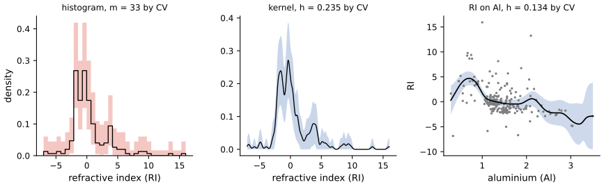
fig_20_S6. Download: PDF · SVGDemonstrations for this chapter
Each demonstration runs in the browser and links back to these notes. The ▶ Demo boxes above open them already set to the case under discussion.
| Demonstration | What you can see | Sections and results |
|---|---|---|
| How many bins? Cross-validation for a histogram | Histograms of the redshifts, the glass data or simulated data with any number of bins; the cross-validation score (20.14) against \(m\), its minimiser and flat range; the envelope (20.17); for simulated data the exact expected score. Presets: 1 Figure 20.3; 2 oversmoothed; 3 undersmoothed; 4 Figure 20.4; 5 score against exact risk; 6 Exercise 20.2. | 20.2; Theorems 20.4, 20.7, 20.10 |
| Kernel regression with a confidence band | Nadaraya-Watson or local linear fits to the WMAP spectrum, the motorcycle data or the glass data; the one-fit cross-validation curves of both estimators; \(\hs\) from differences; the band (20.37) and the degrees of freedom. Presets: 1 Figure 20.8; 2 undersmoothed; 3 oversmoothed; 4 Figure 20.9; 5 non-constant noise; 6 local linear. | 20.4; Theorem 20.22; Filling the gaps 20.15, 20.17, 20.18 |
| Histogram or kernel? The rates \(n^{-2/3}\) and \(n^{-4/5}\) | Exact bias, variance and risk against the width for four Normal mixtures; optimal risks against \(n\) with simulated replicates; the \(d\)-dimensional rate and Silverman's table. Presets: 1 two rates; 2 Figure 20.2; 3 simulation; 4 a hard density; 5 \(d=5\). | 20.1–20.3; Theorems 20.4, 20.14; Filling the gap 20.13 |
Related demonstrations in the companion courses: the local regression demo and the kernel density bandwidth demo of Statistical Learning: Theory and Methods, and the kernel density demo of Statistical Methods for Modern Biology. The Python code that produces every figure of this page is code/ch20_nonparametric_curve_estimation.py (see the code index).
References
- Wasserman, L. (2004). All of Statistics: A Concise Course in Statistical Inference. Springer, New York. Chapter 20, pp. 303–326. www.stat.cmu.edu/~larry/all-of-statistics.
- Bickel, P. J. and Rosenblatt, M. (1973). On some global measures of the deviations of density function estimates. The Annals of Statistics, 1(6), 1071–1095.
- Bowman, A. W. (1984). An alternative method of cross-validation for the smoothing of density estimates. Biometrika, 71(2), 353–360.
- Buja, A., Hastie, T. and Tibshirani, R. (1989). Linear smoothers and additive models. The Annals of Statistics, 17(2), 453–510.
- Chaudhuri, P. and Marron, J. S. (1999). SiZer for exploration of structures in curves. Journal of the American Statistical Association, 94(447), 807–823.
- Fan, J. and Gijbels, I. (1996). Local Polynomial Modelling and Its Applications. Chapman and Hall, London.
- Hall, P. and Marron, J. S. (1987). Extent to which least-squares cross-validation minimises integrated square error in nonparametric density estimation. Probability Theory and Related Fields, 74(4), 567–581.
- Härdle, W. (1990). Applied Nonparametric Regression. Cambridge University Press, Cambridge.
- Loader, C. (1999). Local Regression and Likelihood. Springer, New York.
- Marron, J. S. and Wand, M. P. (1992). Exact mean integrated squared error. The Annals of Statistics, 20(2), 712–736.
- Rice, J. (1984). Bandwidth choice for nonparametric regression. The Annals of Statistics, 12(4), 1215–1230.
- Rudemo, M. (1982). Empirical choice of histograms and kernel density estimators. Scandinavian Journal of Statistics, 9(2), 65–78.
- Scott, D. W. (1992). Multivariate Density Estimation: Theory, Practice, and Visualization. Wiley, New York.
- Silverman, B. W. (1986). Density Estimation for Statistics and Data Analysis. Chapman and Hall, London.
- Stone, C. J. (1984). An asymptotically optimal window selection rule for kernel density estimates. The Annals of Statistics, 12(4), 1285–1297.
- Tsybakov, A. B. (2009). Introduction to Nonparametric Estimation. Springer, New York.
The numerical statements in the text (the cross-validation shortcuts against brute force, the exact unbiasedness of both scores, the exact and asymptotic risks and optimal widths, the kernel efficiencies, the rounding threshold, Silverman's table, the design bias, the variance of a linear smoother, the consistency of the difference estimator, the coverage limits and simulations, and the solutions of the exercises) were confirmed numerically.