Diffusion Models
A diffusion model learns to generate data by learning to undo noise. A fixed Markov chain adds a little Gaussian noise to a data vector at each of \(T\) steps until nothing of it is left; a neural network is then trained to take one step back, and new data are made by starting from pure noise and stepping back \(T\) times. Section 20.1 studies the noising chain, which has closed forms for everything that matters; Section 20.2 derives the training objective from the evidence lower bound and shows that it reduces to predicting the noise that was added; Section 20.3 shows that this is the same as learning the score \(\nabla\ln p\) of the noised data and connects diffusion models with score matching, Langevin sampling and stochastic differential equations; Section 20.4 steers the generation towards a class or a text prompt.
Ch. 1 Deep learning revolution Ch. 2 Probabilities Ch. 3 Standard distributions Ch. 4 Regression Ch. 5 Classification Ch. 6 Deep neural networks Ch. 7 Gradient descent Ch. 8 Backpropagation Ch. 9 Regularization Ch. 10 Convolutional networks Ch. 11 Structured distributions Ch. 12 Transformers Ch. 13 Graph neural networks Ch. 14 Sampling Ch. 15 Discrete latent variables Ch. 16 Continuous latent variables Ch. 17 GANs Ch. 18 Normalizing flows Ch. 19 Autoencoders Ch. 20 Diffusion models Appendices A to C
How to read these notes
They follow the book. Sections carry the book's numbers (20.1, 20.2.4, ...) and every displayed equation that appears in the book carries the book's own equation number, e.g. (20.37). Equations without a number are steps that the book skips.
Filling the gaps. Wherever the book states a result without proof, says it "can be shown", or leaves it to an exercise, an orange Filling the gap box or a proof gives the full argument. Proofs start hidden: open one with its bar, or use the button below.
Figures and demonstrations. Eight of the nine figures are reproduced by the Python code. Figures 20.3 to 20.6 are computed from explicit densities; Figures 20.1, 20.7, 20.8 and 20.9 show photographs or the output of large published models, so the code reproduces the phenomenon at small scale, with a two-dimensional data set and with 14×14 MNIST digits, and the captions say so. Figure 20.2, a drawing of the graphical model, has no data and is not reproduced. Eight supplementary figures (20.S1 to 20.S8, our own) illustrate the gaps that are filled. Two small networks are trained on one CPU thread: a denoiser for a two-dimensional spiral (about 90 seconds), whose weights also run in the browser demonstrations, and one for 14×14 MNIST (about five minutes). The ▶ Demo boxes open an interactive demonstration already set to the case being discussed.
Main reference
C. M. Bishop and H. Bishop, Deep Learning: Foundations and Concepts, Springer (2024), Chapter 20, pages 581–607. Section, equation, figure and exercise numbers below refer to this book. Further reading is listed in the references; the book's website is www.bishopbook.com. There is no official solution for the exercises of this chapter; all solutions below are my own.
The explanations, derivations, figures and code are my own; equations are cited by their numbers in the book.
Companion course: Bayesian and Probabilistic Machine Learning
Diffusion models are the subject of Lecture 4 of the companion course's advanced module on deep generative models, which presents the forward chain, the noise-prediction network and the score connection briefly, with two demonstrations that use the exact score of a mixture and no training. This chapter gives the full derivations, trains real networks, and adds the evidence lower bound, deterministic sampling, the SDE view and guidance. The Gaussian identities it rests on are proved in full there.
- Diffusion models: Advanced topics, lecture 4 (here Sections 20.1–20.3), with the demonstrations denoising diffusion on a swirl and linear and cosine noise schedules.
- The variational autoencoder and its evidence lower bound: Advanced topics, lecture 1, and the bound in general: Section 10.1 (here 20.2.2); normalising flows, which the probability-flow ODE turns a diffusion model into: lecture 2 (here 20.3.4).
- Conditional and marginal Gaussians and Bayes' theorem for linear-Gaussian models, used for (20.6) and (20.15): Result 2.9, Result 2.11, Result 2.12 and completing the square, Filling the gap 2.3 (here 20.1.1, 20.1.2); the KL divergence between Gaussians: Result 2.13 (here Result 20.6).
- Kernel density estimators, the "Parzen" smoothing of Section 20.3.2: Section 2.5.1; Markov chains: Section 11.2.
The chapter at a glance
- 20.1 Each noising step is a linear-Gaussian map, so \(t\) of them compose into one: \(\bz_t=\sqrt{\alpha_t}\bx+\sqrt{1-\alpha_t}\beps\) (Result 20.2). The chain forgets \(\bx\) exactly when \(\sum_t\beta_t=\infty\). Given \(\bx\), the reverse step is Gaussian with mean and variance (20.16)–(20.17) (Result 20.3).
- 20.2 Without \(\bx\) the reverse step is Gaussian only when \(\beta_t\) is small, with mean \(\bz_t+\beta_t(\bz_t/2+\nabla\ln q)\) (Result 20.4). The evidence lower bound splits into a reconstruction term, a prior term and \(T-1\) consistency terms (Result 20.5), each a weighted squared error between predicted and true noise (Result 20.7). Whatever the weights, the best predictor is \(\E[\beps\given\bz_t]=-\sqrt{1-\alpha_t}\,\nabla\ln q(\bz_t)\) (Result 20.8), so the network learns a rescaled score. Algorithm 20.2 and the deterministic DDIM update are two samplers for the same network (Filling the gap 20.4).
- 20.3 Explicit, implicit and denoising score matching differ by constants (Results 20.10 and 20.11); denoising score matching is the noise-prediction loss. Plain Langevin sampling cannot get the weights of separated modes right, and a ladder of noise levels fixes this (Filling the gap 20.6). In continuous time the chain is an SDE, and an ODE with the same marginals turns the model into a flow with an exact likelihood (Result 20.13).
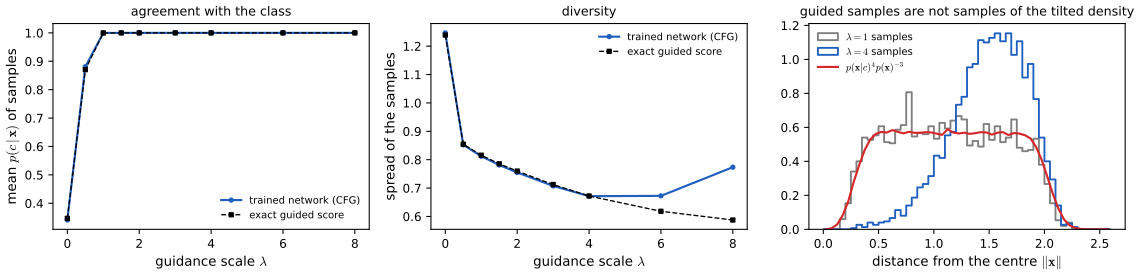
- 20.4 Classifier guidance and classifier-free guidance are the same score when both are exact (Result 20.14); they trade diversity for agreement with the class, and guided samples are not samples from \(p(\bx\given c)^\lambda p(\bx)^{1-\lambda}\) (Filling the gap 20.7).
Notation. \(\bx\in\R^D\) is a data vector and \(\bz_1,\dots,\bz_T\) the noised versions; \(\beta_t\in(0,1)\) is the noise variance of step \(t\) and \(\alpha_t=\prod_{\tau\le t}(1-\beta_\tau)\) (20.7) (in the literature often \(\bar\alpha_t\)); \(\alpha_0=1\). \(q\) denotes the fixed forward (noising) distributions and \(p(\cdot\given\bw)\) the learned reverse ones; \(q_t(\bz)=q(\bz_t=\bz)\) is the marginal of \(\bz_t\) when \(\bx\) is drawn from the data. \(g(\bz,\bw,t)\) is the noise-prediction network and \(\bs(\bz,\bw)\) a score network. The demonstrations and figures use \(T=200\) steps with \(\beta_t\) rising linearly from \(10^{-3}\) to \(0.05\), so \(\alpha_T=0.0056\).
Printings. The first printing has several slips in this chapter, among them a subscript \(t\) for \(1\) in (20.39) and Algorithm 20.2, a missing \(1/L\) in (20.28), a wrong definition of \(\beps\) in (20.52), swapped names in the discussion of Exercise 20.7, a caption of Figure 20.7 that does not match (20.60), and \(\nabla_\bx p\) for \(\nabla_\bx\ln p\) in Exercise 20.14. Each is flagged where it occurs, and the list with the evidence is in the summary before the exercises.
pp. 581–582 Generative models of the kind met in Chapters 16 to 19 draw a latent vector from a simple distribution and push it through a network. Diffusion models, also called denoising diffusion probabilistic models (Sohl-Dickstein et al., 2015; Ho, Jain and Abbeel, 2020), fit the same pattern with two twists: the "encoder" from data to latent is not learned but fixed (a noising process), and the latent space has the same dimension as the data. They can be read as hierarchical variational autoencoders with a fixed encoder (Luo, 2022). They are easy to train and give excellent samples; their weakness is that generation needs many sequential passes through the network.

20.1 Forward Encoder
See also the companion course, Advanced topics, lecture 4 (the forward chain), and its noise-schedules demo.
pp. 582–583 Take a data vector \(\bx\) and blend it with Gaussian noise, independently in each coordinate:
\[ \bz_1=\sqrt{1-\beta_1}\,\bx+\sqrt{\beta_1}\,\beps_1,\qquad \beps_1\sim\N(\beps_1\given\bzero,\bI), \tag{20.1} \]with \(\beta_1<1\), which is the same as
\[ q(\bz_1\given\bx)=\N(\bz_1\given\sqrt{1-\beta_1}\,\bx,\ \beta_1\bI). \tag{20.2} \]Repeating with fresh noise gives \(\bz_2,\dots,\bz_T\):
\[ \bz_t=\sqrt{1-\beta_t}\,\bz_{t-1}+\sqrt{\beta_t}\,\beps_t, \tag{20.3} \] \[ q(\bz_t\given\bz_{t-1})=\N(\bz_t\given\sqrt{1-\beta_t}\,\bz_{t-1},\ \beta_t\bI). \tag{20.4} \]The \(\beta_t\in(0,1)\) are set by hand, usually increasing with \(t\) (the noise schedule). The conditionals (20.4) form a Markov chain, drawn as a graphical model in the book's Figure 20.2 (a chain \(\bx\to\bz_1\to\dots\to\bz_T\); not reproduced). In the literature the data are often called \(\bx_0\) and the latents \(\bx_1,\dots,\bx_T\).
The book says that the coefficients \(\sqrt{1-\beta_t}\) and \(\sqrt{\beta_t}\) pull the mean towards zero and the covariance towards the identity. The precise statement:
Result 20.1 (one noising step contracts towards \(\N(\bzero,\bI)\)) pp. 582–584, (20.3); Exercises 20.1, 20.2, 20.5
If \(\bz_{t-1}\) has mean \(\bmu\) and covariance \(\Sig\) (any distribution), then \(\bz_t\) in (20.3) has
\[ \E[\bz_t]=\sqrt{1-\beta_t}\,\bmu,\qquad \cov[\bz_t]=(1-\beta_t)\Sig+\beta_t\bI,\qquad \cov[\bz_t]-\bI=(1-\beta_t)(\Sig-\bI). \]So \(\|\E[\bz_t]\|=\sqrt{1-\beta_t}\,\|\bmu\|\) and, in any matrix norm, \(\|\cov[\bz_t]-\bI\|=(1-\beta_t)\|\Sig-\bI\|\): both distances shrink. In particular zero mean and unit covariance are preserved exactly, and \(\N(\bzero,\bI)\) is the stationary distribution of every step. Given \(\bz_{t-1}\), (20.3) is a constant plus a scaled standard Gaussian, which is (20.4); for \(t=1\) it is (20.2).
Proof
\(\beps_t\) has mean \(\bzero\), covariance \(\bI\) and is independent of \(\bz_{t-1}\). By linearity, \(\E[\bz_t]\)
Numerical experiments verify the moment map by simulation (400 000 draws, covariance within 0.01) and the preservation of zero mean and unit covariance for a uniform \(\bz_{t-1}\): Gaussianity is not needed for the moments.
20.1.1 Diffusion kernel
pp. 583–584 By the Markov property the joint distribution of the latents given \(\bx\) is
\[ q(\bz_1,\dots,\bz_t\given\bx)=q(\bz_1\given\bx)\prod_{\tau=2}^tq(\bz_\tau\given\bz_{\tau-1}). \tag{20.5} \]Integrating out \(\bz_1,\dots,\bz_{t-1}\) gives the diffusion kernel
\[ q(\bz_t\given\bx)=\N(\bz_t\given\sqrt{\alpha_t}\,\bx,\ (1-\alpha_t)\bI), \tag{20.6} \] \[ \alpha_t=\prod_{\tau=1}^t(1-\beta_\tau), \tag{20.7} \]or, as a recipe,
\[ \bz_t=\sqrt{\alpha_t}\,\bx+\sqrt{1-\alpha_t}\,\beps_t,\qquad\beps_t\sim\N(\bzero,\bI), \tag{20.8} \]where \(\beps_t\) is now the total noise, not the noise of step \(t\). This is what makes training cheap: any \(\bz_t\) can be drawn in one shot without running the chain.
Result 20.2 (the diffusion kernel) p. 583, (20.5)–(20.8); Exercise 20.3
For every \(t\ge1\), \(q(\bz_t\given\bx)\) is (20.6) with \(\alpha_t\) from (20.7). More generally, for \(s<t\), \(q(\bz_t\given\bz_s)\)
Proof (by induction, as Exercise 20.3 asks)
Base case. For \(t=1\), \(\alpha_1=1-\beta_1\), and (20.6) is (20.2).
Induction step. Suppose \(\bz_t=\sqrt{\alpha_t}\,\bx+\sqrt{1-\alpha_t}\,\bu\) with \(\bu\sim\N(\bzero,\bI)\) independent of the future noise \(\beps_{t+1}\). By (20.3), \[ \bz_{t+1}=\sqrt{1-\beta_{t+1}}\sqrt{\alpha_t}\,\bx+\Big[\sqrt{(1-\beta_{t+1})(1-\alpha_t)}\,\bu+\sqrt{\beta_{t+1}}\,\beps_{t+1}\Big]. \] The first coefficient is \(\sqrt{\alpha_{t+1}}\) by (20.7). The bracket is a sum of two independent zero-mean Gaussians, which is Gaussian with the sum of the covariances (the book's (3.212); companion Result 2.12): \[ (1-\beta_{t+1})(1-\alpha_t)+\beta_{t+1}=1-(1-\beta_{t+1})\alpha_t=1-\alpha_{t+1}. \] So \(\bz_{t+1}=\sqrt{\alpha_{t+1}}\,\bx+\sqrt{1-\alpha_{t+1}}\,\bu'\) with \(\bu'\sim\N(\bzero,\bI)\), which is (20.6) at \(t+1\). The general statement follows in the same way starting the chain at \(\bz_s\), since \(\prod_{\tau=s+1}^t(1-\beta_\tau)=\alpha_t/\alpha_s\). ∎
Numerical experiments confirm the two coefficient identities for all 200 steps of our schedule to \(10^{-14}\), and that 100 000 chains run for 60 steps have the mean and variance of (20.6).
Filling the gap 20.1: when does the chain forget the data? p. 584, (20.9)–(20.10); Exercise 20.4
The book says that \(q(\bz_T\given\bx)\to\N(\bz_T\given\bzero,\bI)\) as \(T\to\infty\), and hence that the marginal \(q(\bz_T)\) is \(\N(\bzero,\bI)\). Both statements need a condition, and for finite \(T\) both are approximations whose error can be computed.
Derivation
The condition. By (20.6) the kernel tends to \(\N(\bzero,\bI)\) if and only if \(\alpha_T\to0\). Since \(\ln\alpha_T=\sum_{t\le T}\ln(1-\beta_t)\) and \(\beta\le-\ln(1-\beta)\le\beta/(1-\beta)\), \(\alpha_T\to0\) if and only if \(\sum_t\beta_t=\infty\). This holds if, for instance, \(\beta_t\ge b>0\) for all \(t\) (then \(\alpha_T\le(1-b)^T\)). It fails for a summable schedule: with \(\beta_t=1/(t+1)^2\), the product telescopes, \(\prod_{t=1}^N\big(1-\tfrac1{(t+1)^2}\big)\)
The error for finite \(T\). The KL divergence between two Gaussians (companion Result 2.13) gives \[ \KL\big(q(\bz_T\given\bx)\,\|\,\N(\bzero,\bI)\big)=\tfrac12\Big[\alpha_T\|\bx\|^2-D\alpha_T-D\ln(1-\alpha_T)\Big]=\tfrac12\alpha_T\|\bx\|^2+O(D\alpha_T^2). \] For the marginal, \(q(\bz_T)=\int q(\bz_T\given\bx)p(\bx)\,\d\bx\) and the KL divergence is jointly convex, so \[ \KL(q(\bz_T)\|\N(\bzero,\bI))\le\E_\bx\KL(q(\bz_T\given\bx)\|\N(\bzero,\bI)). \] With our schedule (\(\alpha_T=0.0056\)) and the spiral data, the bound is \(4.5\times10^{-3}\) nats. This is the term that the book's ELBO drops (Exercise 20.10, Result 20.5); it is small but not zero, and it is why some schedules are designed to reach \(\alpha_T=0\) exactly.
Why "further updates leave it unchanged". This is the invariance of \(\N(\bzero,\bI)\) in Result 20.1; the contraction factor \(1-\beta_t\) also shows that the covariance converges geometrically.
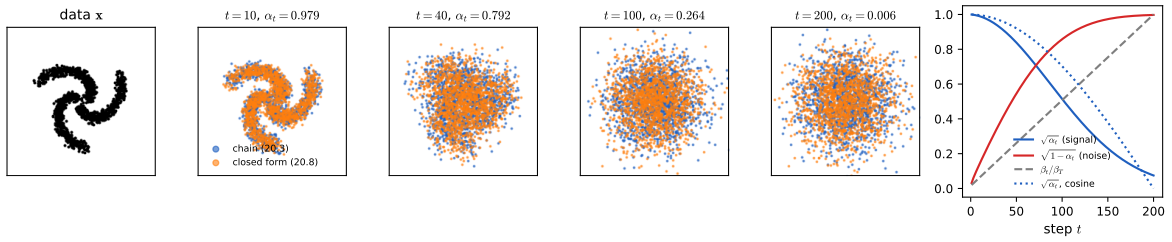
The forward process is analogous to the encoder of a variational autoencoder, except that it is fixed. (In the normalising-flow literature "forward" means the opposite direction, from latent to data.)
20.1.2 Conditional distribution
pp. 584–585 To undo the noise we would like the reverse conditional, by Bayes' theorem
\[ q(\bz_{t-1}\given\bz_t)=\frac{q(\bz_t\given\bz_{t-1})\,q(\bz_{t-1})}{q(\bz_t)}, \tag{20.11} \] \[ q(\bz_{t-1})=\int q(\bz_{t-1}\given\bx)\,p(\bx)\,\d\bx, \tag{20.12} \]but (20.12) requires the unknown data density \(p(\bx)\); with the training set in its place it is a mixture of \(N\) Gaussians, and (20.11) is a complicated mixture. Conditioning on \(\bx\) as well makes everything Gaussian:
\[ q(\bz_{t-1}\given\bz_t,\bx)=\frac{q(\bz_t\given\bz_{t-1},\bx)\,q(\bz_{t-1}\given\bx)}{q(\bz_t\given\bx)}, \tag{20.13} \] \[ q(\bz_t\given\bz_{t-1},\bx)=q(\bz_t\given\bz_{t-1}) \tag{20.14} \](the Markov property), and completing the square gives
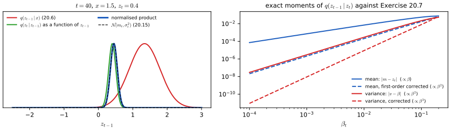
\[ q(\bz_{t-1}\given\bz_t,\bx)=\N\big(\bz_{t-1}\given\bm_t(\bx,\bz_t),\ \sigma_t^2\bI\big), \tag{20.15} \] \[ \bm_t(\bx,\bz_t)=\frac{(1-\alpha_{t-1})\sqrt{1-\beta_t}\,\bz_t+\sqrt{\alpha_{t-1}}\,\beta_t\,\bx}{1-\alpha_t}, \tag{20.16} \] \[ \sigma_t^2=\frac{\beta_t(1-\alpha_{t-1})}{1-\alpha_t}. \tag{20.17} \]Result 20.3 (the reverse conditional given the data) p. 585, (20.13)–(20.17); Exercise 20.6
For \(t\ge2\), \(q(\bz_{t-1}\given\bz_t,\bx)\) is the Gaussian (20.15) with mean (20.16) and variance (20.17). The mean is a convex-type combination of the two pieces of evidence (the coefficients of \(\bz_t/\sqrt{1-\beta_t}\) and of \(\sqrt{\alpha_{t-1}}\bx\) are \((1-\beta_t)(1-\alpha_{t-1})/(1-\alpha_t)\) and \(\beta_t/(1-\alpha_t)\), which add to 1), and \(\sigma_t^2<\beta_t\), with \(\sigma_t^2/\beta_t=(1-\alpha_{t-1})/(1-\alpha_t)\to1\) as \(\alpha_t\to0\). By convention \(\alpha_0=1\), which makes (20.17) give \(\sigma_1^2=0\): \(\bz_0=\bx\) is known.
Proof (completing the square)
As a function of \(\bz_{t-1}\) the denominator of (20.13) is constant. Taking logarithms of the numerator, with (20.4) and (20.6) at \(t-1\), and keeping only terms that depend on \(\bz_{t-1}\):
\[ \ln q(\bz_{t-1}\given\bz_t,\bx)=-\frac{\|\bz_t-\sqrt{1-\beta_t}\,\bz_{t-1}\|^2}{2\beta_t}-\frac{\|\bz_{t-1}-\sqrt{\alpha_{t-1}}\,\bx\|^2}{2(1-\alpha_{t-1})}+\const. \]
Expanding the squares, the quadratic part is \(-\tfrac12\lambda\|\bz_{t-1}\|^2\) and the linear part is \(\bz_{t-1}^\T\mathbf{b}\) with
\[ \lambda=\frac{1-\beta_t}{\beta_t}+\frac1{1-\alpha_{t-1}}=\frac{(1-\beta_t)(1-\alpha_{t-1})+\beta_t}{\beta_t(1-\alpha_{t-1})}=\frac{1-\alpha_t}{\beta_t(1-\alpha_{t-1})}, \qquad \mathbf{b}=\frac{\sqrt{1-\beta_t}}{\beta_t}\bz_t+\frac{\sqrt{\alpha_{t-1}}}{1-\alpha_{t-1}}\bx, \]
where the numerator of \(\lambda\) was simplified as in the proof of Result 20.2. Completing the square, \(-\tfrac12\lambda\|\bz_{t-1}\|^2+\bz_{t-1}^\T\mathbf b\)
A second route. Given \(\bx\), the pair \((\bz_{t-1},\bz_t)\) is jointly Gaussian with variances \(1-\alpha_{t-1}\) and \(1-\alpha_t\) and cross-covariance \(\sqrt{1-\beta_t}(1-\alpha_{t-1})\) per coordinate; the conditional-Gaussian formulas (the book's Section 3.2.4; here Result 3.7, companion Result 2.9) give the same mean and variance. Numerical experiments confirm both routes, and a direct quadrature of the normalised product, to \(10^{-14}\) at \(t=2,40,150,200\).
20.2 Reverse Decoder
pp. 585–587 Since \(q(\bz_{t-1}\given\bz_t)\) is intractable, the reverse step is learned: a distribution \(p(\bz_{t-1}\given\bz_t,\bw)\) defined by a network plays the role of the VAE's decoder. When is a Gaussian a good model for it? By (20.11), \(q(\bz_{t-1}\given\bz_t)\)
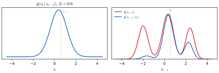
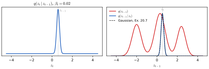
The book says that a Taylor expansion makes this precise (Exercise 20.7), and that the variance of the reverse step is then close to \(\beta_t\). Here is the expansion, with the first corrections.
Result 20.4 (the reverse step for small \(\beta_t\)) pp. 586–587; Exercise 20.7
Let \(q_{t-1}=q(\bz_{t-1})\) be smooth and positive, and write \(\bs=\nabla\ln q_{t-1}(\bz_t)\) and \(\mathbf H=\nabla\nabla^\T\ln q_{t-1}(\bz_t)\) for its score and Hessian at the point \(\bz_t\). As \(\beta=\beta_t\to0\), \(q(\bz_{t-1}\given\bz_t)\) is approximately Gaussian with
\[ \E[\bz_{t-1}\given\bz_t]=\bz_t+\beta\big(\tfrac12\bz_t+\bs\big)+O(\beta^2),\qquad \cov[\bz_{t-1}\given\bz_t]=\beta\bI+\beta^2(\bI+\mathbf H)+O(\beta^3). \]To lowest order: mean \(\bz_t\), covariance \(\beta_t\bI\), the covariance of the forward step, as the book states. The first correction to the mean is a step up the score, the first correction to the covariance depends on the curvature of \(\ln q_{t-1}\).
Proof
Write \(\bz_{t-1}=\bz_t+\boldsymbol\delta\). From (20.11) and (20.4), \[ \ln q(\bz_{t-1}\given\bz_t)=-\frac{\|\bz_t-\sqrt{1-\beta}(\bz_t+\boldsymbol\delta)\|^2}{2\beta}+\ln q_{t-1}(\bz_t+\boldsymbol\delta)+\const. \] Expand the second term to second order, \(\ln q_{t-1}(\bz_t)+\bs^\T\boldsymbol\delta+\tfrac12\boldsymbol\delta^\T\mathbf H\boldsymbol\delta\). Collect powers of \(\boldsymbol\delta\): the quadratic coefficient is \(-\tfrac12\boldsymbol\delta^\T\Lambda\boldsymbol\delta\) with precision \(\Lambda=\frac{1-\beta}\beta\bI-\mathbf H\), and the linear coefficient is \(\mathbf b^\T\boldsymbol\delta\) with \(\mathbf b=\frac{\sqrt{1-\beta}(1-\sqrt{1-\beta})}{\beta}\bz_t+\bs\). The Gaussian with this exponent has covariance \(\Lambda^{-1}\) and mean \(\bz_t+\Lambda^{-1}\mathbf b\).
Covariance. \(\Lambda^{-1}\)
Mean. \(\sqrt{1-\beta}(1-\sqrt{1-\beta})/\beta=\tfrac12+O(\beta)\), so \(\mathbf b=\tfrac12\bz_t+\bs+O(\beta)\) and \(\Lambda^{-1}\mathbf b=\beta(\tfrac12\bz_t+\bs)+O(\beta^2)\).
The neglected terms. Under the Gaussian, \(\boldsymbol\delta=O(\sqrt\beta)\), so the cubic Taylor term of \(\ln q_{t-1}\) is \(O(\beta^{3/2})\) in the exponent; it shifts the mean by \(O(\beta^2)\) (a third moment of \(\boldsymbol\delta\) times \(\Lambda^{-1}=O(\beta)\)) and the covariance by \(O(\beta^3)\), so neither stated order is affected. ∎
Figure 20.S2(b) confirms the orders with the exact moments of the one-dimensional mixture: the error of the corrected mean falls like \(\beta^2\) and that of the corrected variance like \(\beta^3\) (fitted slopes 1.99 and 3.00). Note the form of the mean: \(\bz_t+\beta(\tfrac12\bz_t+\nabla\ln q)\) is one Euler step of the reverse-time SDE of Section 20.3.4, and the same expression reappears in Result 20.9.
p. 587 So the reverse step is modelled as
\[ p(\bz_{t-1}\given\bz_t,\bw)=\N\big(\bz_{t-1}\given\bmu(\bz_t,\bw,t),\ \beta_t\bI\big), \tag{20.18} \]where one network \(\bmu(\bz_t,\bw,t)\), with the step index as an extra input, serves for every step; its output has the dimension of its input, so for images a U-net is the usual choice (Section 10.5.4). The variance could also be learned (Nichol and Dhariwal, 2021); Ho, Jain and Abbeel (2020) found the two fixed choices \(\beta_t\) and \(\sigma_t^2\) of (20.17) to work about equally well, and Result 20.3 shows they differ only for small \(t\). The whole generative model is
\[ p(\bx,\bz_1,\dots,\bz_T\given\bw)=p(\bz_T)\Big\{\prod_{t=2}^Tp(\bz_{t-1}\given\bz_t,\bw)\Big\}\,p(\bx\given\bz_1,\bw), \tag{20.19} \]with \(p(\bz_T)=\N(\bz_T\given\bzero,\bI)\), which equals \(q(\bz_T)\) only approximately (Filling the gap 20.1). Sampling is ancestral: draw \(\bz_T\), then each \(\bz_{t-1}\) in turn, then \(\bx\).
20.2.1 Training the decoder
p. 587 The likelihood of a data point integrates over all noise trajectories,
\[ p(\bx\given\bw)=\int\!\cdots\!\int p(\bx,\bz_1,\dots,\bz_T\given\bw)\,\d\bz_1\dots\d\bz_T, \tag{20.20} \]an instance of the latent-variable model (16.81) with \(\bz=(\bz_1,\dots,\bz_T)\), all of the data's dimension (as in a normalising flow, unlike a VAE or GAN). The integral is intractable.
20.2.2 Evidence lower bound
See also the companion course, Section 10.1 (the variational lower bound) and Advanced topics, lecture 1 (the VAE).
pp. 588–589 For any distribution \(q(\bz)\),
\[ \ln p(\bx\given\bw)=\mathcal L(\bw)+\KL\big(q(\bz)\,\|\,p(\bz\given\bx,\bw)\big), \tag{20.21} \] \[ \mathcal L(\bw)=\int q(\bz)\ln\Big\{\frac{p(\bx,\bz\given\bw)}{q(\bz)}\Big\}\d\bz, \tag{20.22} \] \[ \KL\big(f(\bz)\,\|\,g(\bz)\big)=-\int f(\bz)\ln\Big\{\frac{g(\bz)}{f(\bz)}\Big\}\d\bz, \tag{20.23} \]which follows from the product rule
\[ p(\bx,\bz\given\bw)=p(\bz\given\bx,\bw)\,p(\bx\given\bw) \tag{20.24} \](proof in Result 20.5; KL divergence: Section 2.5.5). Since \(\KL\ge0\),
\[ \ln p(\bx\given\bw)\ge\mathcal L(\bw). \tag{20.25} \]In a VAE \(q\) has its own parameters, and optimising them tightens the bound. In a diffusion model \(q\) is the fixed forward chain \(q(\bz_1,\dots,\bz_T\given\bx)\) of (20.5), which depends on \(\bx\); only the reverse model is trained. Substituting (20.5) and (20.19),
\[ \mathcal L(\bw)=\E_q\Big[\ln\frac{p(\bz_T)\{\prod_{t=2}^Tp(\bz_{t-1}\given\bz_t,\bw)\}p(\bx\given\bz_1,\bw)}{q(\bz_1\given\bx)\prod_{t=2}^Tq(\bz_t\given\bz_{t-1},\bx)}\Big]=\E_q\Big[\ln p(\bz_T)+\sum_{t=2}^T\ln\frac{p(\bz_{t-1}\given\bz_t,\bw)}{q(\bz_t\given\bz_{t-1},\bx)}-\ln q(\bz_1\given\bx)+\ln p(\bx\given\bz_1,\bw)\Big], \tag{20.26} \] \[ \E_q[\,\cdot\,]\equiv\int\!\cdots\!\int q(\bz_1\given\bx)\prod_{t=2}^Tq(\bz_t\given\bz_{t-1})\,[\,\cdot\,]\,\d\bz_1\dots\d\bz_T. \tag{20.27} \]The first and third terms do not depend on \(\bw\). The fourth is the reconstruction term of a VAE, estimated by sampling \(\bz_1\):
\[ \E_q[\ln p(\bx\given\bz_1,\bw)]\simeq\frac1L\sum_{l=1}^L\ln p(\bx\given\bz_1^{(l)},\bw),\qquad\bz_1^{(l)}\sim\N(\sqrt{1-\beta_1}\,\bx,\beta_1\bI). \tag{20.28} \](The book's (20.28) omits the factor \(1/L\).) No reparameterisation is needed, because \(q\) has no parameters to differentiate.
Filling the gap 20.2: why the ELBO is rewritten before it is estimated p. 589
The book says that estimating the second term of (20.26) with sampled pairs \((\bz_{t-1},\bz_t)\) is correct but noisy, and rewrites the bound so that each term needs a single sample. The reason is a standard variance-reduction principle.
Derivation
Conditioning reduces variance. For any random variables \(U,V\) and function \(f\), the law of total variance gives \(\var[f(U,V)]\)
Applied here. The rewritten bound (20.32) is exactly of this kind: the term \(\ln\{p(\bz_{t-1}\given\bz_t,\bw)/q(\bz_{t-1}\given\bz_t,\bx)\}\), averaged over \(\bz_{t-1}\) given \(\bz_t\) (and \(\bx\)), is minus a KL divergence between two Gaussians, available in closed form (Result 20.6). Only \(\bz_t\) remains to be sampled, from the kernel (20.6). The per-sample variance of the pairwise estimator is large because \(\ln p(\bz_{t-1}\given\bz_t)\) contains \(\|\bz_{t-1}-\bmu\|^2/2\beta_t\), whose fluctuation is of order \(D\) (a scaled \(\chi^2_D\) variable); the closed-form KL removes that fluctuation entirely.
20.2.3 Rewriting the ELBO
pp. 589–591 The network models the reverse direction while \(q\) runs forward, so turn the forward factor around with Bayes' theorem (conditioning on \(\bx\) keeps it tractable):
\[ q(\bz_t\given\bz_{t-1},\bx)=\frac{q(\bz_{t-1}\given\bz_t,\bx)\,q(\bz_t\given\bx)}{q(\bz_{t-1}\given\bx)}, \tag{20.29} \] \[ \ln\frac{p(\bz_{t-1}\given\bz_t,\bw)}{q(\bz_t\given\bz_{t-1},\bx)}=\ln\frac{p(\bz_{t-1}\given\bz_t,\bw)}{q(\bz_{t-1}\given\bz_t,\bx)}+\ln\frac{q(\bz_{t-1}\given\bx)}{q(\bz_t\given\bx)}. \tag{20.30} \]Dropping terms free of \(\bw\),
\[ \mathcal L(\bw)=\E_q\Big[\sum_{t=2}^T\ln\frac{p(\bz_{t-1}\given\bz_t,\bw)}{q(\bz_{t-1}\given\bz_t,\bx)}+\ln p(\bx\given\bz_1,\bw)\Big], \tag{20.31} \] \[ \mathcal L(\bw)=\underbrace{\int q(\bz_1\given\bx)\ln p(\bx\given\bz_1,\bw)\,\d\bz_1}_{\text{reconstruction term}}-\underbrace{\sum_{t=2}^T\int\KL\big(q(\bz_{t-1}\given\bz_t,\bx)\,\|\,p(\bz_{t-1}\given\bz_t,\bw)\big)\,q(\bz_t\given\bx)\,\d\bz_t}_{\text{consistency terms}}. \tag{20.32} \]Result 20.5 (the ELBO of a diffusion model, with nothing dropped) pp. 588–590, (20.21)–(20.32); Exercises 20.8, 20.9, 20.10
- (20.21) holds for every density \(q(\bz)\) for which the integrals exist.
- With \(q\) the forward chain, the complete bound (keeping every term the book drops) is \[ \mathcal L=\E_{q(\bz_1|\bx)}[\ln p(\bx\given\bz_1,\bw)]-\sum_{t=2}^T\E_{q(\bz_t|\bx)}\Big[\KL\big(q(\bz_{t-1}\given\bz_t,\bx)\,\|\,p(\bz_{t-1}\given\bz_t,\bw)\big)\Big]-\KL\big(q(\bz_T\given\bx)\,\|\,p(\bz_T)\big). \] The last term (the book's (20.63), which enters with a minus sign) is free of \(\bw\), and is small but positive for finite \(T\) (Filling the gap 20.1).
Proof
(1) Insert (20.24) into (20.22): \(\mathcal L\)
(2) Insert (20.30) into (20.26). The second piece of (20.30), summed over \(t=2,\dots,T\), telescopes:
\[ \sum_{t=2}^T\ln\frac{q(\bz_{t-1}\given\bx)}{q(\bz_t\given\bx)}=\ln q(\bz_1\given\bx)-\ln q(\bz_T\given\bx). \]
The \(\ln q(\bz_1\given\bx)\) cancels the third term of (20.26), and \(\ln p(\bz_T)-\ln q(\bz_T\given\bx)\), averaged over \(q\), is \(-\KL(q(\bz_T\given\bx)\|p(\bz_T))\) because only \(\bz_T\) appears. In the reconstruction term only \(\bz_1\) appears, so the other factors of (20.27) integrate to 1 (integrate out \(\bz_T\), then \(\bz_{T-1}\), and so on), leaving the integral against \(q(\bz_1\given\bx)\). For the \(t\)-th consistency term only \(\bz_{t-1}\) and \(\bz_t\) appear; their joint density under (20.27) is \(q(\bz_{t-1},\bz_t\given\bx)\)
Both sides are evaluated for a one-dimensional chain with \(T=5\) and a linear reverse model: \(10^6\) Monte Carlo draws of \(\ln\{p(x,\bz)/q(\bz\given x)\}\) give \(-1.5331\pm0.0009\), the closed form \(-1.5337\). Part (1) is checked to \(10^{-10}\) on a linear-Gaussian model with an arbitrary \(q\).
The consistency terms compare two Gaussians, (20.15) and (20.18), so they are available in closed form:
\[ \KL\big(q(\bz_{t-1}\given\bz_t,\bx)\,\|\,p(\bz_{t-1}\given\bz_t,\bw)\big)=\frac1{2\beta_t}\|\bm_t(\bx,\bz_t)-\bmu(\bz_t,\bw,t)\|^2+\const \tag{20.33} \]Result 20.6 (the consistency term in closed form) p. 590, (20.33); Exercise 20.11
For Gaussians in \(\R^D\), \(\KL\big(\N(\bm,\sigma^2\bI)\,\|\,\N(\bmu,\beta\bI)\big)\)
Proof (short; the general formula is companion Result 2.13)
\[ \KL=\E_{\N(\bm,\sigma^2\bI)}\big[\ln\N(\bz\given\bm,\sigma^2\bI)-\ln\N(\bz\given\bmu,\beta\bI)\big]. \] The log densities differ by \(\frac D2\ln\frac\beta{\sigma^2}-\frac{\|\bz-\bm\|^2}{2\sigma^2}+\frac{\|\bz-\bmu\|^2}{2\beta}\). Under the first Gaussian \(\E\|\bz-\bm\|^2=D\sigma^2\) and \(\E\|\bz-\bmu\|^2=D\sigma^2+\|\bm-\bmu\|^2\). Adding up gives the formula. The constant is \(\frac D2(r-1-\ln r)\) with \(r=\sigma_t^2/\beta_t\), nonnegative because \(\ln r\le r-1\). ∎ (Checked against Monte Carlo.)
20.2.4 Predicting the noise
See also the companion course, Advanced topics, lecture 4 (the denoising model predicts the noise).
pp. 591–592 Ho, Jain and Abbeel (2020) obtained better results by letting the network predict the total noise \(\beps_t\) of (20.8) rather than the mean. Solving (20.8) for \(\bx\),
\[ \bx=\frac1{\sqrt{\alpha_t}}\bz_t-\frac{\sqrt{1-\alpha_t}}{\sqrt{\alpha_t}}\beps_t, \tag{20.34} \] \[ \bm_t(\bx,\bz_t)=\frac1{\sqrt{1-\beta_t}}\Big\{\bz_t-\frac{\beta_t}{\sqrt{1-\alpha_t}}\beps_t\Big\}, \tag{20.35} \]and, defining the mean network through a noise network \(g\) in the same way,
\[ \bmu(\bz_t,\bw,t)=\frac1{\sqrt{1-\beta_t}}\Big\{\bz_t-\frac{\beta_t}{\sqrt{1-\alpha_t}}g(\bz_t,\bw,t)\Big\}, \tag{20.36} \] \[ \KL\big(q(\bz_{t-1}\given\bz_t,\bx)\,\|\,p(\bz_{t-1}\given\bz_t,\bw)\big)=\frac{\beta_t}{2(1-\alpha_t)(1-\beta_t)}\big\|g(\sqrt{\alpha_t}\,\bx+\sqrt{1-\alpha_t}\,\beps_t,\bw,t)-\beps_t\big\|^2+\const. \tag{20.37} \]For \(t=1\), with (20.18) also used for \(p(\bx\given\bz_1,\bw)\),
\[ \ln p(\bx\given\bz_1,\bw)=-\frac1{2\beta_1}\|\bx-\bmu(\bz_1,\bw,1)\|^2+\const, \tag{20.38} \] \[ \ln p(\bx\given\bz_1,\bw)=-\frac1{2(1-\beta_1)}\|g(\bz_1,\bw,1)-\beps_1\|^2+\const \tag{20.39} \](the book prints \(1-\beta_t\) in (20.39); it is \(1-\beta_1\)). This is (20.37) at \(t=1\), since \(1-\alpha_1=\beta_1\). Dropping the weights altogether gives the loss that is used in practice,
\[ \mathcal L(\bw)=-\sum_{t=1}^T\big\|g(\sqrt{\alpha_t}\,\bx+\sqrt{1-\alpha_t}\,\beps_t,\bw,t)-\beps_t\big\|^2. \tag{20.40} \]Result 20.7 (the ELBO as weighted noise prediction) pp. 591–592, (20.34)–(20.39); Exercises 20.12, 20.13
(20.35) holds identically; with (20.36), \(\frac1{2\beta_t}\|\bm_t-\bmu\|^2=w_t\|g-\beps_t\|^2\) with \(w_t=\frac{\beta_t}{2(1-\alpha_t)(1-\beta_t)}\), so (20.33) becomes (20.37); and (20.38) becomes (20.39), with \(w_1=\frac1{2(1-\beta_1)}\). Hence, up to terms free of \(\bw\), the bound of Result 20.5 is \(-\sum_{t=1}^Tw_t\,\E\|g(\bz_t,\bw,t)-\beps_t\|^2\).
Proof
(20.35). Insert (20.34) into (20.16). The coefficient of \(\bz_t\) becomes \(\frac{(1-\alpha_{t-1})\sqrt{1-\beta_t}}{1-\alpha_t}+\frac{\sqrt{\alpha_{t-1}}\beta_t}{(1-\alpha_t)\sqrt{\alpha_t}}\). Since \(\sqrt{\alpha_{t-1}}/\sqrt{\alpha_t}=1/\sqrt{1-\beta_t}\), this is \(\frac{(1-\alpha_{t-1})(1-\beta_t)+\beta_t}{(1-\alpha_t)\sqrt{1-\beta_t}}\)
(20.37). Subtracting (20.36) from (20.35), \(\bm_t-\bmu=\frac{\beta_t}{\sqrt{1-\beta_t}\sqrt{1-\alpha_t}}(g-\beps_t)\), so \(\frac1{2\beta_t}\|\bm_t-\bmu\|^2\)
(20.39). With \(\alpha_1=1-\beta_1\), (20.36) at \(t=1\) is \(\bmu=(\bz_1-\sqrt{\beta_1}\,g)/\sqrt{1-\beta_1}\), and by (20.1) \(\bz_1/\sqrt{1-\beta_1}=\bx+\sqrt{\beta_1}\beps_1/\sqrt{1-\beta_1}\). So \(\bx-\bmu=\frac{\sqrt{\beta_1}}{\sqrt{1-\beta_1}}(g-\beps_1)\), and \(\frac1{2\beta_1}\|\bx-\bmu\|^2=\frac1{2(1-\beta_1)}\|g-\beps_1\|^2\). This is \(w_1\), and \(w_t\) at \(t=1\) gives the same value because \(1-\alpha_1=\beta_1\). ∎ (All three identities are checked with random numbers to \(10^{-12}\).)
What does the network learn? The next result is the key fact of the chapter, and the book only hints at it in Section 20.3.2.
Result 20.8 (the best noise predictor is a rescaled score) supplement to pp. 591–592 and 596–597
Let \(\bx\sim p(\bx)\), \(\beps\sim\N(\bzero,\bI)\) independent, \(\bz_t=\sqrt{\alpha_t}\bx+\sqrt{1-\alpha_t}\beps\), and \(q_t\) the density of \(\bz_t\). Among all functions \(g(\bz,t)\), the loss \(\sum_t w_t\,\E\|g(\bz_t,t)-\beps\|^2\), for any positive weights \(w_t\), is minimised by
\[ g^\star(\bz,t)=\E[\beps\given\bz_t=\bz]=-\sqrt{1-\alpha_t}\,\nabla_\bz\ln q_t(\bz), \]and the excess loss of any \(g\) is \(\sum_tw_t\,\E\|g(\bz_t,t)-g^\star(\bz_t,t)\|^2\). Equivalently, \(\E[\bx\given\bz_t=\bz]=\big(\bz+(1-\alpha_t)\nabla\ln q_t(\bz)\big)/\sqrt{\alpha_t}\) (Tweedie's formula).
Proof
Minimiser. For each \(t\) separately, \(\E\|g(\bz_t)-\beps\|^2\)
The score. \(q_t(\bz)=\int p(\bx)\,\N(\bz\given\sqrt{\alpha_t}\bx,(1-\alpha_t)\bI)\,\d\bx\). Differentiating under the integral (allowed because the Gaussian and its gradient are bounded and integrable), with \(\nabla_\bz\N(\bz\given\sqrt{\alpha_t}\bx,(1-\alpha_t)\bI)\)
For the spiral the posterior over \(\bx\) is a Gaussian mixture, so both sides can be computed independently; they agree to \(4\times10^{-14}\). The trained network (three hidden layers of 64 units) has \(\E\|g-g^\star\|^2=0.0068\) against an irreducible loss \(\E\|g^\star-\beps\|^2=0.614\), and the decomposition above holds within Monte Carlo error.
Filling the gap 20.3: why the weights can be dropped, and what dropping them does p. 592, (20.40)
The book reports that omitting \(w_t\) improves results empirically. Result 20.8 explains why this is safe, and the size of the weights explains why it helps.
Derivation
Same target. A flexible enough network minimises every per-step loss at \(g^\star\), whatever the weights; the weights only decide how a network of limited capacity trades errors between steps, and how the stochastic gradients are scaled.
What the ELBO weights do. With our schedule \(w_1=0.50\), \(w_{10}=0.077\), \(w_{50}=0.022\), and \(w_t\) stays between \(0.018\) and \(0.027\) for \(t\ge50\) (Figure 20.S3(a)): the true bound spends most of its weight on the first few steps, where the noise is barely visible and the task (recovering imperceptible noise) matters least for sample quality. The unweighted loss gives every step equal weight, which up-weights the large-\(t\) steps where the coarse structure of the sample is decided.
The unweighted loss is denoising score matching with a natural weighting. With \(\bs=-g/\sqrt{1-\alpha_t}\) and the kernel score \(-\beps_t/\sqrt{1-\alpha_t}\) of (20.53), \(\|g-\beps_t\|^2=(1-\alpha_t)\,\|\bs-\nabla\ln q(\bz_t\given\bx)\|^2\). So (20.40) is the multi-level score-matching loss (20.54) with \(\lambda(t)=\sigma_t^2=1-\alpha_t\), the noise variance: exactly the choice of Song and Ermon (2019), made so that each term has about the same magnitude (the kernel score has size \(\sqrt{D/\sigma^2}\)).
Stochastic gradients. Algorithm 20.1 samples \(t\) uniformly; with the ELBO weights the weights vary by a factor of 28 between steps (Figure 20.S3(a)), so its variance would be dominated by the rare small-\(t\) draws. Equal weights avoid that, which is another reason the simple loss trains well. (Importance-sampling \(t\) in proportion to \(w_t\) is the alternative when the true bound is wanted, for example to report likelihoods.)
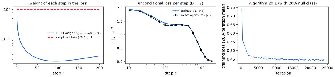
In words, (20.40) says: take a data point, pick a step, add the corresponding amount of noise in one shot, and ask the network to name the noise. Each reuse of a training point comes with fresh noise, a built-in form of data augmentation. Stochastic gradient descent samples one \(t\) per data point:
Algorithm 20.1 (training a denoising diffusion probabilistic model) p. 593
- Input: data \(\{\bx_n\}\), schedule \(\beta_1,\dots,\beta_T\). Compute \(\alpha_t=\prod_{\tau\le t}(1-\beta_\tau)\).
- Repeat until converged: draw \(\bx\) from the data, \(t\) uniformly from \(\{1,\dots,T\}\) and \(\beps\sim\N(\bzero,\bI)\); set \(\bz_t=\sqrt{\alpha_t}\bx+\sqrt{1-\alpha_t}\beps\); take an optimiser step on \(\|g(\bz_t,\bw,t)-\beps\|^2\) (averaged over a mini-batch).
- Return \(\bw\).
The code (train_denoiser) adds two common details: an exponential moving average of the weights, which is the network that is used, and, for guidance, the class input replaced by a null class 20% of the time (Section 20.4.2).
20.2.5 Generating new samples
pp. 592–594 Starting from \(\bz_T\sim\N(\bzero,\bI)\), each step evaluates \(g(\bz_t,\bw,t)\), forms the mean (20.36) and adds noise:
\[ \bz_{t-1}=\bmu(\bz_t,\bw,t)+\sqrt{\beta_t}\,\beps,\qquad\beps\sim\N(\bzero,\bI). \tag{20.41} \]Although \(g\) estimates the total noise, only the fraction \(\beta_t/\sqrt{1-\alpha_t}\) of it is subtracted from \(\bz_t\) (the book says "from \(\bz_{t-1}\)"), the result is rescaled by \(1/\sqrt{1-\beta_t}\), and new noise of variance \(\beta_t\) is added. The last step adds no noise.
Algorithm 20.2 (sampling from a denoising diffusion probabilistic model) p. 594
- Draw \(\bz_T\sim\N(\bzero,\bI)\).
- For \(t=T,\dots,2\): \(\bmu=\frac1{\sqrt{1-\beta_t}}\big\{\bz_t-\frac{\beta_t}{\sqrt{1-\alpha_t}}g(\bz_t,\bw,t)\big\}\); draw \(\beps\sim\N(\bzero,\bI)\); \(\bz_{t-1}=\bmu+\sqrt{\beta_t}\,\beps\).
- Return \(\bx=\frac1{\sqrt{1-\beta_1}}\big\{\bz_1-\frac{\beta_1}{\sqrt{1-\alpha_1}}g(\bz_1,\bw,1)\big\}\). (The book writes \(g(\bz_1,\bw,t)\) in this line; the step index is 1.)
On a sub-sequence of steps \(\tau_S>\dots>\tau_1=1\) (used by the demo), the same update applies with \(\beta\) replaced by \(1-\alpha_{\tau_i}/\alpha_{\tau_{i-1}}\), the variance of the composite forward step (Result 20.2).
Result 20.9 (what one sampling step does) supplement to p. 592, (20.36), (20.41)
With the optimal predictor \(g^\star\) of Result 20.8, the mean (20.36) is exactly the posterior mean of the reverse step, \(\bmu(\bz_t)=\E[\bz_{t-1}\given\bz_t]\), and
\[ \bmu(\bz_t)=\frac{\bz_t+\beta_t\nabla\ln q_t(\bz_t)}{\sqrt{1-\beta_t}}=\bz_t+\beta_t\big(\tfrac12\bz_t+\nabla\ln q_t(\bz_t)\big)+O(\beta_t^2), \]which agrees with the small-\(\beta\) expansion of Result 20.4 to the order stated there (the scores of \(q_t\) and \(q_{t-1}\) differ by \(O(\beta_t)\)). So each step of Algorithm 20.2 is a shrink-and-climb step: a gradient step of size \(\beta_t\) up the log density of the current noise level, plus a slight expansion that undoes the contraction of (20.3), plus noise of variance \(\beta_t\), a Langevin-like move (compare (14.61) in Section 14.3.3).
Proof
By the tower rule and the Markov property, \(\E[\bz_{t-1}\given\bz_t]\)
Filling the gap 20.4: deterministic sampling with DDIM p. 594 (Song, Meng and Ermon, 2020)
The book mentions that denoising diffusion implicit models "relax the Markovian assumption on the noise process while retaining the same objective" and sample one or two orders of magnitude faster. Here is the construction and why the same network can be used.
Derivation
Only the marginals matter for training. The loss (20.40) involves only the one-step kernels \(q(\bz_t\given\bx)\) of (20.6), not the joint distribution of the chain. Any family of processes with the same kernels has the same loss and the same optimal \(g^\star\).
A family with the same kernels. For a pair of steps \(t'<t\) and any \(0\le s^2\le1-\alpha_{t'}\), define \[ q_s(\bz_{t'}\given\bz_t,\bx)=\N\Big(\sqrt{\alpha_{t'}}\,\bx+\sqrt{1-\alpha_{t'}-s^2}\,\frac{\bz_t-\sqrt{\alpha_t}\bx}{\sqrt{1-\alpha_t}},\ s^2\bI\Big). \] If \(\bz_t=\sqrt{\alpha_t}\bx+\sqrt{1-\alpha_t}\beps\), the fraction is \(\beps\), so \(\bz_{t'}=\sqrt{\alpha_{t'}}\bx+\sqrt{1-\alpha_{t'}-s^2}\,\beps+s\,\beps'\) with \(\beps'\) independent: a Gaussian with mean \(\sqrt{\alpha_{t'}}\bx\) and variance \((1-\alpha_{t'}-s^2)+s^2=1-\alpha_{t'}\). So \(q(\bz_{t'}\given\bx)\) is again (20.6), for every \(s\).
The sampler. Replace \(\bx\) by the network's estimate \(\hat\bx=(\bz_t-\sqrt{1-\alpha_t}\,g)/\sqrt{\alpha_t}\) (Tweedie's formula with \(g\)) and \(\beps\) by \(g\): \[ \bz_{t'}=\sqrt{\alpha_{t'}}\,\hat\bx+\sqrt{1-\alpha_{t'}-s^2}\;g(\bz_t,\bw,t)+s\,\beps',\qquad s=\eta\sqrt{\frac{1-\alpha_{t'}}{1-\alpha_t}}\sqrt{1-\frac{\alpha_t}{\alpha_{t'}}}. \] With \(\eta=1\) and \(t'=t-1\), \(s^2=\sigma_t^2\) of (20.17) and the mean equals \(\bm_t(\hat\bx,\bz_t)\): the stochastic sampler with the posterior variance (checked to \(10^{-15}\)). With \(\eta=0\) no noise is added after \(\bz_T\): the sampler is a deterministic map from noise to data (DDIM).
Why big steps work. In the variables \(\bar\bz=\bz/\sqrt{\alpha}\) and \(\rho=\sqrt{(1-\alpha)/\alpha}\), the \(\eta=0\) update reads \(\bar\bz_{t'}=\bar\bz_t+(\rho_{t'}-\rho_t)\,g(\bz_t,\bw,t)\): one Euler step of the ODE \(\d\bar\bz/\d\rho=g\), which is the probability-flow ODE (20.57) in these variables (Result 20.13). A smooth ODE can be integrated with few large steps; the stochastic sampler, whose every step adds noise that the next step must remove, cannot. With the trained spiral network, 20 deterministic steps give a mean log density of the samples of \(-2.04\) against \(-2.94\) for 20 steps of Algorithm 20.2 (real data: \(-1.53\)); 5 steps are too few (\(-4.05\)), 200 give \(-1.85\).
Algorithm 20.3 (DDIM sampling on \(S\) steps) supplement to p. 594
- Choose steps \(T=\tau_S>\dots>\tau_1=1\) and \(\eta\in[0,1]\). Draw \(\bz\sim\N(\bzero,\bI)\).
- For \(i=S,\dots,2\), with \(t=\tau_i\), \(t'=\tau_{i-1}\): \(g=g(\bz,\bw,t)\), \(\hat\bx=(\bz-\sqrt{1-\alpha_t}g)/\sqrt{\alpha_t}\), \(s\) as above, \(\bz\leftarrow\sqrt{\alpha_{t'}}\hat\bx+\sqrt{1-\alpha_{t'}-s^2}\,g+s\beps\).
- Return \(\hat\bx=(\bz-\sqrt{1-\alpha_1}g(\bz,\bw,1))/\sqrt{\alpha_1}\).
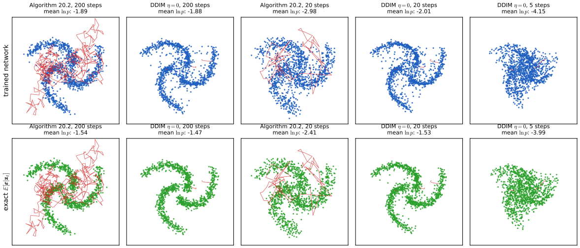
Two further remarks of the book: generation can be sped up by viewing the denoising as a differential equation and using better solvers (Section 20.3.4), and the framework extends to discrete data with discrete noise processes (Austin et al., 2021), for example to choose atom types when generating molecules.
20.3 Score Matching
See also in this course, Section 14.3.1 (energies and scores) and Result 14.18 (contrastive divergence is score matching); in the companion course, Advanced topics, lecture 4 (score matching).
pp. 594–595 A second family of generative models, developed largely independently (Hyvärinen, 2005; Song and Ermon, 2019), is built on the score (or Stein score)
\[ \bs(\bx)=\nabla_\bx\ln p(\bx), \tag{20.42} \]a gradient with respect to the data, not the parameters, with one component per component of \(\bx\) (for an image, an image of the same size). If two densities have the same score everywhere, integrating gives \(q(\bx)=Kp(\bx)\); so a model of the score determines the density up to a constant, which is never needed for sampling with Langevin dynamics.
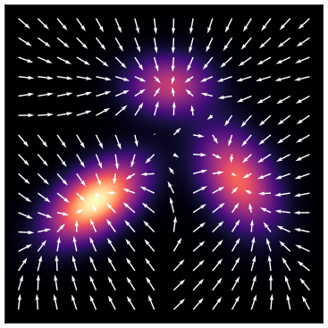
20.3.1 Score loss function
pp. 595–596 The obvious loss compares the model score with the data score,
\[ J(\bw)=\frac12\int\|\bs(\bx,\bw)-\nabla_\bx\ln p(\bx)\|^2\,p(\bx)\,\d\bx, \tag{20.43} \]and, as for energy-based models (Section 14.3.1), the score needs no normalisation. The network can output the \(D\) components of \(\bs\) directly, or a scalar \(\phi(\bx)\) whose gradient is computed by automatic differentiation; the book notes that the second is more expensive and that the first is usual.
Filling the gap 20.5: two ways to represent a score, and when equal scores mean equal densities pp. 595–596; Exercises 20.14, 20.15
A direct network with \(D\) outputs is in general not the gradient of anything; a gradient network always is, at a constant-factor extra cost. And "equal scores imply \(q=Kp\)" needs a connected domain.
Derivation
Which vector fields are scores. If \(\bs=\nabla\phi\) with \(\phi\) twice continuously differentiable, then \(\partial s_i/\partial x_j=\partial^2\phi/\partial x_j\partial x_i=\partial s_j/\partial x_i\) (symmetry of second derivatives), so the matrix \(M_{ij}=\partial s_i/\partial x_j-\partial s_j/\partial x_i\) of (20.64) vanishes. Conversely, on \(\R^D\) (or any simply connected domain) a field with \(M\equiv0\) is a gradient (Poincaré's lemma). A network with \(D\) outputs has an arbitrary Jacobian, of which only the diagonal of \(M\) is automatically zero; numerically, \(\max|M_{ij}|=0.14\) for a small random network with three outputs, against \(7\times10^{-18}\) for the gradient of a scalar network.
Cost. Let one forward pass cost \(W\) operations (about the number of weights). The direct score costs \(O(W)\). The gradient score costs one forward and one backward pass, still \(O(W)\) (reverse-mode differentiation gives all \(D\) partial derivatives of a scalar for a constant multiple of the forward cost; Chapter 8). Training is where the difference shows: the loss contains \(\nabla_\bx\phi\), so its gradient with respect to \(\bw\) needs a backward pass through the backward pass ("double backpropagation"), roughly two to three times the cost of training the direct network: a constant factor, not a factor \(D\). A direct computation confirms that double backpropagation gives the right parameter gradient (agreement with finite differences to \(10^{-6}\)). The expensive object is different: the divergence \(\nabla\!\cdot\bs\) of Exercise 20.16 needs one backward pass per input dimension, \(O(DW)\).
Equal scores. If \(\nabla\ln q=\nabla\ln p\) on an open set \(\Omega\), then \(\ln q-\ln p\) has zero gradient there and is constant on each connected component of \(\Omega\). If both densities are positive everywhere, \(\Omega=\R^D\) is connected and \(q=Kp\); since both integrate to 1, \(K=1\). If the supports are disjoint pieces, the constant can differ from piece to piece: the score carries no information about the relative weights of the pieces. That is Exercise 20.18, and the reason for Section 20.3.3.
20.3.2 Modified score loss
pp. 596–597 (20.43) contains the unknown \(\nabla\ln p\). The data give only the empirical distribution
\[ p_{\mathcal D}(\bx)=\frac1N\sum_{n=1}^N\delta(\bx-\bx_n), \tag{20.44} \] \[ \delta(\bx)=0,\quad\bx\ne\bzero, \tag{20.45} \] \[ \int\delta(\bx)\,\d\bx=1, \tag{20.46} \]which has no score. Smoothing it with a noise kernel gives a Parzen (kernel density) estimate (Section 3.5.2; companion Section 2.5.1),
\[ q_\sigma(\bz)=\int q(\bz\given\bx,\sigma)\,p(\bx)\,\d\bx, \tag{20.47} \] \[ q(\bz\given\bx,\sigma)=\N(\bz\given\bx,\sigma^2\bI), \tag{20.48} \] \[ J(\bw)=\frac12\int\|\bs(\bz,\bw)-\nabla_\bz\ln q_\sigma(\bz)\|^2\,q_\sigma(\bz)\,\d\bz, \tag{20.49} \]and, the key step (Vincent, 2011),
\[ J(\bw)=\frac12\iint\|\bs(\bz,\bw)-\nabla_\bz\ln q(\bz\given\bx,\sigma)\|^2\,q(\bz\given\bx,\sigma)\,p(\bx)\,\d\bz\,\d\bx+\const, \tag{20.50} \] \[ J(\bw)=\frac1{2N}\sum_{n=1}^N\int\|\bs(\bz,\bw)-\nabla_\bz\ln q(\bz\given\bx_n,\sigma)\|^2\,q(\bz\given\bx_n,\sigma)\,\d\bz+\const. \tag{20.51} \]The target in (20.50) is the score of the kernel, which is known:
\[ \nabla_\bz\ln q(\bz\given\bx,\sigma)=-\frac1\sigma\beps,\qquad\beps=\frac{\bz-\bx}\sigma\sim\N(\bzero,\bI) \tag{20.52} \](the book defines \(\beps=\bz-\bx\) here, which would make the score \(-\beps/\sigma^2\); with the standardised \(\beps\) the formula \(-\beps/\sigma\) is right). For the diffusion kernel (20.6),
\[ \nabla_\bz\ln q(\bz\given\bx)=-\frac1{\sqrt{1-\alpha_t}}\beps. \tag{20.53} \]So denoising score matching asks \(\bs(\bz_t,\bw)\) to predict \(-\beps/\sqrt{1-\alpha_t}\): it is the noise-prediction loss with \(\bs=-g/\sqrt{1-\alpha_t}\), and its minimiser is the score of the noised density (Result 20.8).
Result 20.10 (implicit score matching; Hyvärinen, 2005) Exercise 20.16, (20.65)–(20.68)
If \(p\) and \(\bs(\cdot,\bw)\) are differentiable and \(p(\bx)s_i(\bx,\bw)\to0\) as \(\|\bx\|\to\infty\), then
\[ J(\bw)=\int\Big[\nabla\!\cdot\bs(\bx,\bw)+\frac12\|\bs(\bx,\bw)\|^2\Big]p(\bx)\,\d\bx+\frac12\int\|\nabla\ln p\|^2p\,\d\bx,\qquad\nabla\!\cdot\bs=\sum_{i=1}^D\frac{\partial s_i(\bx,\bw)}{\partial x_i}. \]The first integral needs only samples from \(p\), not its score. (In the book's (20.66) the divergence is written as \(\sum_i\partial^2\ln p/\partial x_i^2\), which is the divergence of the true score; for the model it is \(\sum_i\partial s_i(\bx,\bw)/\partial x_i\).)
Proof
Expand the square in (20.43): \(J=\frac12\E_p\|\bs\|^2-\E_p[\bs^\T\nabla\ln p]+\frac12\E_p\|\nabla\ln p\|^2\). The last term is the constant. For the cross term use \(p\nabla\ln p=\nabla p\) and integrate by parts one coordinate at a time, (20.67)–(20.68): \[ \int s_i\,\frac{\partial p}{\partial x_i}\,\d\bx=\Big[s_ip\Big]_{x_i=-\infty}^{\infty}-\int p\,\frac{\partial s_i}{\partial x_i}\,\d\bx=-\int p\,\frac{\partial s_i}{\partial x_i}\,\d\bx, \] the boundary term vanishing by assumption. Summing over \(i\): \(-\E_p[\bs^\T\nabla\ln p]=\E_p[\nabla\!\cdot\bs]\). ∎
For a linear score model on the one-dimensional mixture, a direct computation gives \(J(\bw)-\E[\nabla\!\cdot\bs+\frac12\|\bs\|^2]=1.919923\) for four random \(\bw\), equal to \(\frac12\E\|\nabla\ln p\|^2\). The divergence is what makes this loss expensive in high dimension: it needs \(D\) backward passes (sliced score matching, Song et al. 2019, estimates it with random projections).
Result 20.11 (denoising score matching is explicit score matching plus a constant; Vincent, 2011) p. 596, (20.47)–(20.51); Exercise 20.17
For any kernel \(q(\bz\given\bx,\sigma)\) and any \(\bs(\cdot,\bw)\) with finite losses, (20.49) and the double integral in (20.50) differ by a constant free of \(\bw\):
\[ J_{\rm DSM}(\bw)-J_{\rm ESM}(\bw)=\frac12\Big(\E_{p(\bx)q(\bz|\bx)}\|\nabla_\bz\ln q(\bz\given\bx,\sigma)\|^2-\E_{q_\sigma}\|\nabla\ln q_\sigma\|^2\Big)\ge0, \]which for the Gaussian kernel (20.48) is \(\frac12\big(D/\sigma^2-\E_{q_\sigma}\|\nabla\ln q_\sigma\|^2\big)\). Both losses therefore have the same minimiser, \(\bs=\nabla\ln q_\sigma\).
Proof
Expand both squares. The terms in \(\|\bs\|^2\) agree: \(\iint\|\bs(\bz)\|^2q(\bz\given\bx)p(\bx)\,\d\bz\,\d\bx\)
Figure 20.S5 and a direct computation: for the one-dimensional mixture and a linear score model, \(J_{\rm DSM}-J_{\rm ESM}\) is the same for every \(\bw\) to \(10^{-8}\) and equals the formula (4.522 at \(\sigma=0.3\), 0.584 at \(\sigma=0.8\)).
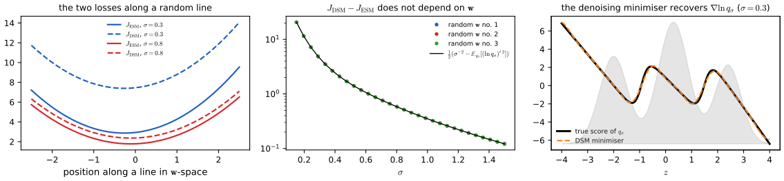
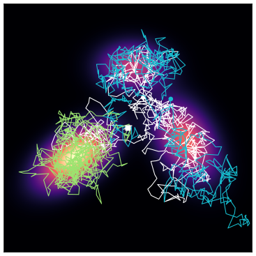
p. 597 Once a score model is trained, Langevin dynamics (Section 14.3.3, (14.61)) samples from it using only the score:
20.3.3 Noise variance
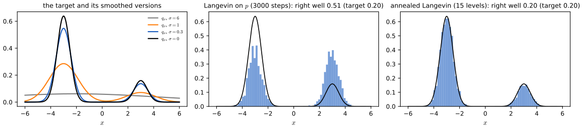
pp. 597–598 Learning the score at a single small noise level has three problems (Song and Ermon, 2019): on a low-dimensional data manifold the density and its score are undefined off the manifold; where data are rare the loss, weighted by the density, says little about the score; and Langevin dynamics cannot get the proportions of separated modes right (Exercise 20.18). A large \(\sigma\) cures all three but distorts the density; a ladder \(\sigma_1^2<\sigma_2^2<\dots<\sigma_L^2\) gets both, with one network \(\bs(\bz,\bw,\sigma^2)\) trained on
\[ \frac12\sum_{i=1}^L\lambda(i)\int\big\|\bs(\bz,\bw,\sigma_i^2)-\nabla_\bz\ln q(\bz\given\bx_n,\sigma_i)\big\|^2\,q(\bz\given\bx_n,\sigma_i)\,\d\bz \tag{20.54} \]per data point. This is the noise-prediction loss of Section 20.2 in another guise (Filling the gap 20.3: \(\lambda(i)=\sigma_i^2\) gives (20.40)). Sampling runs a few Langevin steps at each level from \(\sigma_L\) down to \(\sigma_1\): annealed Langevin dynamics, the analogue of Algorithm 20.2.
Filling the gap 20.6: why Langevin dynamics gets the weights of separated modes wrong, and how annealing fixes it p. 598; Exercise 20.18
Derivation
The score forgets the weights. Let \(p=\lambda p_A+(1-\lambda)p_B\) with disjoint supports. At a point \(\bx\) where \(p_A>0\), \(p_B=0\) in a neighbourhood, so \(\nabla\ln p=\nabla\ln(\lambda p_A)=\nabla\ln p_A\): \(\lambda\) has disappeared. The same holds approximately for components that overlap only in their far tails. Langevin dynamics uses nothing but the score, so a chain started in \(A\) stays in \(A\) for a time that grows exponentially with the barrier, and the fraction of chains in each mode is the fraction that started there, not \(\lambda\).
Smoothing reconnects the modes. \(q_\sigma=\lambda\,(p_A*\N_\sigma)+(1-\lambda)(p_B*\N_\sigma)\) is positive everywhere and, for \(\sigma\) comparable with the distance between the modes, unimodal-looking; its score does depend on \(\lambda\), and Langevin chains cross freely. Decreasing \(\sigma\) slowly, each level starts from samples that are already close to \(q_{\sigma}\) with the right proportions, and the local moves at the smaller \(\sigma\) only have to sharpen each mode.
Step sizes. At level \(\sigma\) the density has length scale at least \(\sigma\), so a step \(\eta_i\propto\sigma_i^2\) keeps the number of steps needed to cross it constant (Song and Ermon's rule \(\eta_i=\epsilon\,\sigma_i^2/\sigma_1^2\)); the Langevin bias of Result 14.16, a relative variance error of about \(\eta/2\sigma^2\), is then the same at every level.
Numbers (Figure 20.S6). Two wells at \(\pm3\) with weights 0.8 and 0.2 and standard deviation 0.5. From uniform starting points on \([-8,8]\), 3000 Langevin steps leave 0.505 of the chains in the right well (0.511 started there). Fifteen levels from \(\sigma=6\) to \(0.1\), 200 steps each with \(\eta=0.1\sigma^2\), give 0.198.
Algorithm 20.4 (annealed Langevin dynamics) p. 598 (Song and Ermon, 2019)
- Input a score model \(\bs(\bz,\sigma)\), levels \(\sigma_L>\dots>\sigma_1\), steps \(K\) per level, a constant \(\epsilon\). Initialise \(\bz\) (for example uniformly or from \(\N(\bzero,\sigma_L^2\bI)\)).
- For \(i=L,\dots,1\): set \(\eta=\epsilon\,\sigma_i^2\); repeat \(K\) times: \(\bz\leftarrow\bz+\eta\,\bs(\bz,\sigma_i)+\sqrt{2\eta}\,\beps\).
- Return \(\bz\).
20.3.4 Stochastic differential equations
See also the companion course, Advanced topics, lecture 2 (normalising flows and the change of variables).
pp. 598–599 Letting the number of steps go to infinity while each \(\beta_t\) shrinks with the step size turns the chain into a stochastic differential equation (Song et al., 2020), of the general form
\[ \d\bz=\underbrace{\bf(\bz,t)\,\d t}_{\text{drift}}+\underbrace{g(t)\,\d\bv}_{\text{diffusion}}, \tag{20.55} \]with \(\bv\) a standard Brownian motion (independent Gaussian increments of variance \(\d t\)). For the forward process (Exercise 20.19) this is
\[ \d\bz=-\tfrac12\beta(t)\,\bz\,\d t+\sqrt{\beta(t)}\,\d\bv. \tag{20.70} \]Each forward SDE has a reverse-time SDE (Anderson, 1982),
\[ \d\bz=\big[\bf(\bz,t)-g^2(t)\nabla_\bz\ln p_t(\bz)\big]\d t+g(t)\,\d\bv, \tag{20.56} \]run from \(t=T\) down to \(0\) (so \(\d t<0\)), whose score is that of the time-\(t\) marginal \(p_t\) (the book writes \(p(\bz)\)). Discretising it with equal steps (Euler–Maruyama) gives a Langevin-like update; better solvers exist (Kloeden and Platen, 2013). Every such diffusion also has a deterministic counterpart with the same marginals \(p_t\), the probability-flow ODE
\[ \frac{\d\bz}{\d t}=\bf(\bz,t)-\frac12g^2(t)\nabla_\bz\ln p_t(\bz), \tag{20.57} \]which can be integrated with adaptive solvers in few steps, and which is a (continuous) normalising flow, so the change-of-variables formula (18.1) gives exact likelihoods.
Result 20.12 (the continuous-time limit of the forward chain) p. 599, (20.70); Exercise 20.19
Let \(\beta_t=\beta(t)\Delta t\) for a continuous \(\beta(\cdot)\). Then (20.3) is \(\bz_{t+\Delta t}-\bz_t\)
Proof
\(\sqrt{1-\beta\Delta t}=1-\tfrac12\beta\Delta t+O(\Delta t^2)\), so \(\sqrt{1-\beta_t}\,\bz_t=\bz_t-\tfrac12\beta(t)\bz_t\Delta t+O(\Delta t^2)\), and \(\sqrt{\beta_t}\beps=\sqrt{\beta(t)}\sqrt{\Delta t}\,\beps\). For the marginal, \(\ln\alpha_T\)
With our schedule (\(\beta(s)\) rising linearly from 0.2 to 10 on \(s\in[0,1]\)), the discrete \(\alpha_T\) differs from \(\alpha(1)=e^{-5.1}\) by 8.4% with \(T=200\), 0.85% with \(T=2000\) and 0.085% with \(T=20000\): an \(O(1/T)\) error.
Result 20.13 (the probability-flow ODE has the marginals of the SDE, and an exact likelihood) p. 599, (20.55)–(20.57)
- Let \(p_t\) be the marginal densities of the forward SDE (20.55). The ODE (20.57), with \(\bz(0)\sim p_0\), has \(\bz(t)\sim p_t\) for all \(t\); run backwards from \(\bz(T)\sim p_T\), it ends at \(p_0\).
- Along a solution, \(\frac{\d}{\d t}\ln p_t(\bz(t))=-\nabla\!\cdot\tilde\bf(\bz(t),t)\), where \(\tilde\bf\) is the right-hand side of (20.57). Hence \(\ln p_0(\bz(0))=\ln p_T(\bz(T))+\int_0^T\nabla\!\cdot\tilde\bf\,\d t\), computable by integrating one extra scalar ODE.
- (Stated, not proved here.) The reverse-time SDE (20.56) also has the marginals \(p_t\) (Anderson, 1982).
Proof of (1) and (2), and the idea of (3)
Fokker–Planck. The marginals of (20.55) satisfy \(\partial_tp_t=-\nabla\!\cdot(\bf p_t)+\tfrac12g^2\Delta p_t\). Since \(\Delta p_t=\nabla\!\cdot(\nabla p_t)=\nabla\!\cdot(p_t\nabla\ln p_t)\), this is \[ \partial_tp_t=-\nabla\!\cdot\Big(\big[\bf-\tfrac12g^2\nabla\ln p_t\big]p_t\Big)=-\nabla\!\cdot(\tilde\bf\,p_t). \] Continuity equation. For an ODE \(\dot\bz=\tilde\bf(\bz,t)\) the density \(\rho_t\) of \(\bz(t)\) satisfies exactly \(\partial_t\rho_t=-\nabla\!\cdot(\tilde\bf\rho_t)\) (conservation of probability mass along the flow). With \(\rho_0=p_0\), \(p_t\) and \(\rho_t\) solve the same first-order linear equation with the same initial condition, so \(\rho_t=p_t\) (uniqueness under the usual smoothness and growth conditions). Running the ODE backwards from \(p_T\) retraces the same family. (2) Along a path, \(\frac{\d}{\d t}\ln p_t(\bz(t))=\partial_t\ln p_t+\tilde\bf^\T\nabla\ln p_t\), and the continuity equation divided by \(p_t\) gives \(\partial_t\ln p_t=-\nabla\!\cdot\tilde\bf-\tilde\bf^\T\nabla\ln p_t\); the sum is \(-\nabla\!\cdot\tilde\bf\). (3) The same manipulation with \(\bf-g^2\nabla\ln p_t\) as the drift of a reverse-time diffusion with coefficient \(g\) reproduces the time-reversed Fokker–Planck equation; this is the idea of Anderson's theorem. ∎
Numbers (Figure 20.S7). For the one-dimensional mixture, whose \(p_t\) is known exactly, 4000 paths of the reverse SDE (1000 Euler–Maruyama steps) and of the ODE (200 RK4 steps) both end at the data density (Kolmogorov–Smirnov distances 0.019 and 0.011). Integrating \(\nabla\!\cdot\tilde\bf=-\tfrac12\beta(1+\partial_z^2\ln p_t)\) along the ODE reproduces \(\ln p_0(\bz(0))\) to \(9\times10^{-9}\) when the exact \(p_T\) is used; replacing \(p_T\) by \(\N(0,1)\), as a trained model must, costs a median 0.008 nats, the prior mismatch of Filling the gap 20.1. Integrating the ODE forward again recovers \(\bz(T)\) to \(3\times10^{-11}\): the flow is invertible.
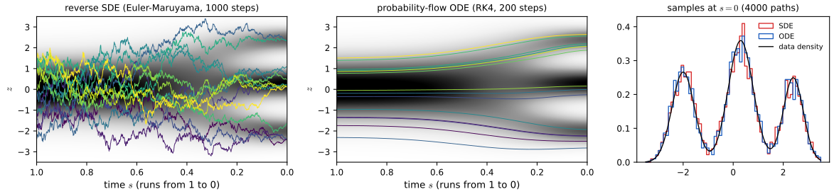
In the variables of Filling the gap 20.4, DDIM with \(\eta=0\) is an Euler method for (20.57), and Algorithm 20.2 a discretisation of (20.56): Euler–Maruyama on the reverse SDE with \(g^2=\beta\) gives \(\bz_{t-1}=\bz_t+\beta_t(\tfrac12\bz_t+\nabla\ln p_t)+\sqrt{\beta_t}\beps\), which is (20.41) with the mean of Result 20.9 to first order.
20.4 Guided Diffusion
pp. 599–600 To sample from a conditional \(p(\bx\given c)\), with \(c\) a class label, a text prompt or a low-resolution image, the simplest approach feeds \(c\) to the network, \(g(\bz,\bw,t,c)\), and trains on pairs \((\bx_n,c_n)\). The network may then give the condition too little weight; guidance is a way to control how much, at the price of diversity.
20.4.1 Classifier guidance
p. 600 With a classifier \(p(c\given\bx)\), Bayes' theorem gives
\[ \nabla_\bx\ln p(\bx\given c)=\nabla_\bx\ln\Big\{\frac{p(c\given\bx)p(\bx)}{p(c)}\Big\}=\nabla_\bx\ln p(\bx)+\nabla_\bx\ln p(c\given\bx), \tag{20.58} \]and a guidance scale \(\lambda\) weights the classifier (Dhariwal and Nichol, 2021):
\[ \mathrm{score}(\bx,c,\lambda)=\nabla_\bx\ln p(\bx)+\lambda\nabla_\bx\ln p(c\given\bx). \tag{20.59} \]\(\lambda=0\) is the unconditional model, \(\lambda=1\) the conditional one, and \(\lambda\gg1\) (say 10) favours samples that the classifier finds easy, at the expense of diversity. The classifier must work on noisy inputs \(\bz_t\), so a separate one has to be trained.
20.4.2 Classifier-free guidance
pp. 600–602 Eliminating the classifier with (20.58) (Exercise 20.20),
\[ \mathrm{score}(\bx,c,\lambda)=\lambda\nabla_\bx\ln p(\bx\given c)+(1-\lambda)\nabla_\bx\ln p(\bx), \tag{20.60} \]a convex combination for \(0<\lambda<1\); for \(\lambda>1\) the unconditional score enters with a negative weight, pushing away from samples that ignore the condition. One network serves for both scores if the condition is replaced by a null value (say \(c=0\)) for 10–20% of the training examples, a dropout of the conditioning input (Section 9.6.1). Classifier-free guidance gives much better results than classifier guidance in practice (Nichol et al., 2021; Saharia et al., 2022), plausibly because a classifier can ignore most of \(\bx\) while a conditional density must account for all of it.
Result 20.14 (the two forms of guidance, in noise-prediction form) pp. 600–601, (20.58)–(20.60); Exercise 20.20
- (20.59) and (20.60) are the same function of \(\bx\) for every \(\lambda\).
- Applied at noise level \(t\) (the only place a diffusion model uses a score), with scores \(-g/\sqrt{1-\alpha_t}\): classifier guidance uses the noise prediction \(g(\bz_t,t)-\lambda\sqrt{1-\alpha_t}\,\nabla\ln p_t(c\given\bz_t)\), and classifier-free guidance uses \(\lambda\,g(\bz_t,t,c)+(1-\lambda)\,g(\bz_t,t,\varnothing)\). If the network and the noisy classifier \(p_t(c\given\bz_t)=q_t(\bz_t\given c)\,p(c)/q_t(\bz_t)\) are exact, the two are identical.
Proof
(1) From (20.58), \(\nabla\ln p(c\given\bx)=\nabla\ln p(\bx\given c)-\nabla\ln p(\bx)\); inserting into (20.59) gives \(\nabla\ln p(\bx)+\lambda\nabla\ln p(\bx\given c)-\lambda\nabla\ln p(\bx)\), which is (20.60). (2) Replace \(p\) by the noised marginals \(q_t(\cdot)\) and \(q_t(\cdot\given c)\) and each score \(\bs\) by \(-g/\sqrt{1-\alpha_t}\); multiplying through by \(-\sqrt{1-\alpha_t}\) gives both forms, and (1) at level \(t\) shows that they agree when exact. ∎
For the spiral all of these are exact Gaussian-mixture quantities; numerically the two forms are equal to \(4\times10^{-15}\), and the noisy-classifier gradient equal to finite differences of \(\ln p_t(c\given\bz_t)\).
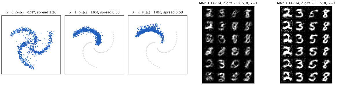
The book's caption to Figure 20.7 calls \(\lambda=0\) "no guidance, just the plain conditional model". Under (20.60) the plain conditional model is \(\lambda=1\) and \(\lambda=0\) ignores the prompt. The caption appears to use the convention \(\mathrm{score}\)
Filling the gap 20.7: what distribution does guidance sample from? pp. 600–601
It is tempting to read (20.60) as the score of \(\tilde p_\lambda(\bx)\)
Derivation
Guidance acts at every noise level. The sampler uses \(\lambda\nabla\ln q_t(\bz\given c)+(1-\lambda)\nabla\ln q_t(\bz)\) at every \(t\). For this to be the score of the noised version of \(\tilde p_\lambda\), noising (a convolution) would have to commute with raising densities to powers, which it does not: the noised version of \(\tilde p_\lambda\) is \(\int\tilde p_\lambda(\bx)\N(\bz\given\sqrt{\alpha_t}\bx,(1-\alpha_t)\bI)\,\d\bx\), while the guided "density" at level \(t\) is \(q_t(\bz\given c)^\lambda q_t(\bz)^{1-\lambda}\), and these differ unless \(\lambda\in\{0,1\}\). So the guided reverse process has no reason to end at \(\tilde p_\lambda\).
What happens instead. At high noise, \(p_t(c\given\bz_t)\) is far from certain wherever the noised classes overlap (for the spiral: near the centre), and the guidance term \(\lambda\nabla\ln p_t(c\given\bz_t)\) pushes the trajectories out of those regions early, when the decision about the coarse position of the sample is made. They never return, even though at \(t=0\) the inner part of the arm is unambiguous (\(p(c\given\bx)\approx1\) there, so \(\tilde p_\lambda\approx p(\bx\given c)\)).
Numbers (Figure 20.S8). With the exact guided score (no network error) and class "arm 1": at \(\lambda=1\) the samples' mean distance from the centre is 1.148, against 1.157 for \(p(\bx\given c)\); at \(\lambda=4\) it is 1.502, against 1.159 for \(\tilde p_4\). Agreement with the class rises from 0.35 (\(\lambda=0\)) to 1.00 (\(\lambda\ge1\)) while the spread falls from 0.82 (\(\lambda=1\)) to 0.67 (\(\lambda=4\)). Beyond \(\lambda\approx4\) the trained network's small errors, multiplied by \(\lambda\), start to show: its spread rises again while the exact one keeps falling.
pp. 601–602 Text and other conditions. A transformer language model (Chapter 12) turns a prompt into a sequence of embeddings that enter the denoiser by concatenation and through cross-attention layers. The same machinery gives super-resolution (denoise a high-resolution sample conditioned on the low-resolution image; Saharia, Ho et al., 2021), cascades of such models (64×64 to 256×256 to 1024×1024; Ho et al., 2021), generation at low resolution followed by learned up-sampling (Nichol et al., 2021; Saharia et al., 2022), and latent diffusion (Rombach et al., 2021), which runs the diffusion in the latent space of a fixed autoencoder trained on clean images and decodes at the end, saving most of the cost of working with full-size images. Inpainting, un-cropping, restoration, colourisation, de-blurring and video generation are further conditional tasks (Yang, Srivastava and Mandt, 2022).
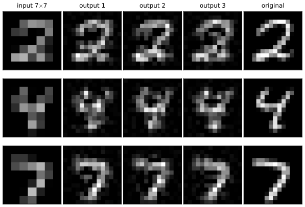
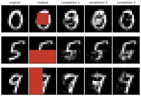
Filling the gap 20.8: conditioning an unconditional model by replacement, and its limits supplement to pp. 601–602, Figures 20.8 and 20.9
Derivation
The idea. Split \(\bz=(\bz^{\rm known},\bz^{\rm free})\) (pixels for inpainting; block averages and the orthogonal detail for super-resolution, since block averaging is a linear projection \(\mathbf P\)). The forward process acts independently on each coordinate, and on orthogonal projections: \(\mathbf P\bz_t=\sqrt{\alpha_t}\mathbf P\bx+\sqrt{1-\alpha_t}\mathbf P\beps\), and \(\mathbf P\beps\) is independent of \((\bI-\mathbf P)\beps\). So the observed part at level \(t\) can be simulated exactly from the observation by (20.8). The replacement sampler runs the reverse chain and after each step overwrites the observed part of \(\bz_{t-1}\) with such a simulation, so that at the end \(\mathbf P\bx\) equals the observation exactly.
Why it is not exact. The correct conditional sampler would draw the free part from \(p(\bz^{\rm free}_{t-1}\given\bz_t,\ \text{observation})\), which requires the score of \(q_t(\bz\given\text{observation})\). Replacement uses the unconditional score and only enforces consistency after the fact; the free part learns about the observation only through the next denoising step, so the two parts can disagree (visible as seams). Remedies include re-noising and repeating steps (Lugmayr et al., 2022) or adding a guidance term built from the observation (in the spirit of Result 20.14); the best results in the book's figures come from models trained with the observation as input.
Summary: errors and imprecisions found in the chapter (first printing)
- p. 584, (20.9) and Exercise 20.4 (imprecision): \(q(\bz_T\given\bx)\to\N(\bzero,\bI)\) needs \(\sum_t\beta_t=\infty\); for \(\beta_t=1/(t+1)^2\) the product \(\alpha_T\to1/2\) (checked). For finite \(T\), \(q(\bz_T)\) is not exactly \(\N(\bzero,\bI)\) (Filling the gap 20.1).
- p. 587: "the reverse distribution \(q(\bz_t\given\bz_{t-1})\) will have a covariance that is close to the covariance \(\beta_t\bI\) of the forward noise process \(q(\bz_{t-1}\given\bz_t)\)": the two conditionals are swapped; the reverse distribution is \(q(\bz_{t-1}\given\bz_t)\) and the forward one \(q(\bz_t\given\bz_{t-1})\). (Also "There considerable flexibility" lacks "is".)
- (20.28): the Monte Carlo estimate needs the factor \(1/L\).
- (20.39): the weight is \(1/2(1-\beta_1)\), not \(1/2(1-\beta_t)\) (it is (20.37) at \(t=1\); checked).
- p. 592: "Substituting this simplified version of (20.37) into (20.33)" should be into (20.32).
- p. 593: the fraction \(\beta_t/\sqrt{1-\alpha_t}\) of the predicted noise is subtracted from \(\bz_t\), not from \(\bz_{t-1}\) (and the result is rescaled by \(1/\sqrt{1-\beta_t}\)).
- Algorithm 20.2, last line: \(g(\bz_1,\bw,t)\) should be \(g(\bz_1,\bw,1)\).
- (20.52): with \(\beps=\bz-\bx\), as written, the score is \(-\beps/\sigma^2\), and \(\beps\) is drawn from \(\N(\bzero,\sigma^2\bI)\), not \(\N(\bz\given\bzero,\bI)\); the formula \(-\beps/\sigma\) holds for the standardised \(\beps=(\bz-\bx)/\sigma\) (checked).
- p. 595 (imprecision): equal scores give \(q=Kp\) only on a connected domain; on disjoint supports the constant may differ between pieces, which is exactly Exercise 20.18 (Filling the gap 20.5).
- p. 599, (20.56)–(20.57): "The SDE given by (20.55) is to be solved in reverse" should refer to (20.56); "for an SDE of the form (20.56), the corresponding ODE is (20.57)" should refer to the forward SDE (20.55); and the score in both is that of the time-dependent marginal, \(\nabla\ln p_t(\bz)\).
- Figure 20.7, caption: "\(\lambda=0\) (no guidance, just the plain conditional model)" contradicts (20.60), where \(\lambda=0\) is the unconditional model and \(\lambda=1\) the plain conditional one; the caption seems to use \(\lambda-1\) as its scale.
- Exercise 20.10: the omitted terms add \(-\KL(q(\bz_T\given\bx)\|p(\bz_T))\) (with a minus sign) to the bound; "\(q(\bz_T\given\bx)\) is equal to \(\N(\bx\given\bzero,\bI)\)" should be \(\N(\bz_T\given\bzero,\bI)\), and holds only in the limit \(T\to\infty\) (with our schedule the term is about \(4.5\times10^{-3}\) nats).
- Exercise 20.14: the score is \(\nabla_\bx\ln p(\bx\given\bw)\), not \(\nabla_\bx p(\bx\given\bw)\) (twice).
- Exercise 20.16, (20.66): the divergence in (20.65) is that of the model, \(\sum_i\partial s_i(\bx,\bw)/\partial x_i\); the second expression \(\sum_i\partial^2\ln p/\partial x_i^2\) is the divergence of the true score. The notation \(s_{\mathcal D}=\nabla\ln p_{\mathcal D}\) is also used for the score of the smooth \(p\).
Exercises
All 20 exercises of Chapter 20 (Bishop and Bishop, 2024, pp. 603–607), restated in my own words, with complete solutions (hidden). Stars give the book's difficulty. The official solutions manual stops at Chapter 10, so these solutions are my own; each numerical statement is confirmed numerically.
Exercise 20.1 (★). From (20.3), express the mean and covariance of \(\bz_t\) through those of \(\bz_{t-1}\), and show that for \(0<\beta_t<1\) the mean moves closer to zero and the covariance closer to \(\bI\).
Solution
\(\E[\bz_t]=\sqrt{1-\beta_t}\,\E[\bz_{t-1}]\) and \(\cov[\bz_t]=(1-\beta_t)\cov[\bz_{t-1}]+\beta_t\bI\), because \(\beps_t\) has mean zero, covariance \(\bI\) and is independent of \(\bz_{t-1}\). Hence \(\|\E[\bz_t]\|\)
\({}=\sqrt{1-\beta_t}\|\E[\bz_{t-1}]\|\) \({}<\|\E[\bz_{t-1}]\|\) unless the mean is already zero, and \(\cov[\bz_t]-\bI=(1-\beta_t)(\cov[\bz_{t-1}]-\bI)\), so every entry and every eigenvalue of the difference shrinks by the factor \(1-\beta_t<1\). Details in Result 20.1. Exercise 20.2 (★). Show that (20.1) is equivalent to (20.2).
Solution
For fixed \(\bx\), \(\bz_1\) is an affine function \(\bm+\mathbf A\beps_1\) of a standard Gaussian with \(\bm=\sqrt{1-\beta_1}\bx\), \(\mathbf A=\sqrt{\beta_1}\bI\). An affine image of a Gaussian is Gaussian, with mean \(\bm\) and covariance \(\mathbf A\mathbf A^\T=\beta_1\bI\); that is (20.2). Conversely, a draw from (20.2) can be written as \(\bm+\sqrt{\beta_1}\beps\) with \(\beps=(\bz_1-\bm)/\sqrt{\beta_1}\sim\N(\bzero,\bI)\). (A Kolmogorov–Smirnov test confirms this.)
Exercise 20.3 (★★★). Prove by induction that the marginal of \(\bz_t\) given \(\bx\) under the forward process is (20.6) with \(\alpha_t\) of (20.7), using the representation (20.3) and the fact that a sum of independent Gaussians is Gaussian with added means and covariances.
Solution
See the proof of Result 20.2: the base case is (20.2), and if \(\bz_t=\sqrt{\alpha_t}\bx+\sqrt{1-\alpha_t}\bu\), then \[ \bz_{t+1}=\sqrt{\alpha_{t+1}}\bx+\big[\sqrt{(1-\beta_{t+1})(1-\alpha_t)}\bu+\sqrt{\beta_{t+1}}\beps_{t+1}\big], \] and the bracket is \(\N(\bzero,(1-\alpha_{t+1})\bI)\) because \((1-\beta_{t+1})(1-\alpha_t)+\beta_{t+1}=1-\alpha_{t+1}\).
Exercise 20.4 (★). Use (20.6) and (20.7) to show that \(q(\bz_T\given\bx)\to\N(\bzero,\bI)\) as \(T\to\infty\).
Solution
If \(\alpha_T\to0\), the mean \(\sqrt{\alpha_T}\bx\to\bzero\) and the covariance \((1-\alpha_T)\bI\to\bI\); Gaussian densities converge pointwise (and in total variation) when their parameters converge, so \(q(\bz_T\given\bx)\to\N(\bzero,\bI)\). Now \(\alpha_T=\prod_{t\le T}(1-\beta_t)\le\exp(-\sum_{t\le T}\beta_t)\) (from \(1-\beta\le e^{-\beta}\)), which tends to zero when \(\sum\beta_t=\infty\), for example when the \(\beta_t\) are bounded below by a positive constant, as for any schedule that is fixed and then repeated, or one whose \(\beta_t\) increase. The condition is needed: for \(\beta_t=1/(t+1)^2\), \(\alpha_T=(T+2)/(2(T+1))\to1/2\) (Filling the gap 20.1).
Exercise 20.5 (★★). For independent random vectors \(\ba,\bb\) and a scalar \(\lambda\), show \(\cov[\ba+\bb]=\cov[\ba]+\cov[\bb]\) (20.61) and \(\cov[\lambda\ba]=\lambda^2\cov[\ba]\) (20.62). Deduce that if \(\bz_{t-1}\) has zero mean and unit covariance then so has \(\bz_t\) of (20.3), whatever \(\beta_t\).
Solution
Let \(\tilde\ba=\ba-\E\ba\), \(\tilde\bb=\bb-\E\bb\). Then \(\cov[\ba+\bb]\)
\({}=\E[(\tilde\ba+\tilde\bb)(\tilde\ba+\tilde\bb)^\T]\) \({}=\cov[\ba]+\cov[\bb]+\E[\tilde\ba\tilde\bb^\T]+\E[\tilde\bb\tilde\ba^\T]\), and by independence \(\E[\tilde\ba\tilde\bb^\T]=\E[\tilde\ba]\E[\tilde\bb]^\T=\mathbf 0\). Also \(\cov[\lambda\ba]=\E[\lambda\tilde\ba\,\lambda\tilde\ba^\T]=\lambda^2\cov[\ba]\). With \(\ba=\sqrt{1-\beta_t}\bz_{t-1}\) and \(\bb=\sqrt{\beta_t}\beps_t\): mean \(\sqrt{1-\beta_t}\cdot\bzero+\bzero=\bzero\) and covariance \((1-\beta_t)\bI+\beta_t\bI=\bI\). No Gaussianity is needed (a simulation with a uniform \(\bz_{t-1}\) confirms this). Exercise 20.6 (★★★). Derive (20.15)–(20.17) from (20.13) by completing the square in \(\bz_{t-1}\).
Solution
The proof of Result 20.3 does exactly this: the exponent is \(-\frac12\lambda\|\bz_{t-1}\|^2+\bz_{t-1}^\T\mathbf b+\const\) with \(\lambda=(1-\alpha_t)/\{\beta_t(1-\alpha_{t-1})\}\) and \(\mathbf b\)
\({}=\frac{\sqrt{1-\beta_t}}{\beta_t}\bz_t+\frac{\sqrt{\alpha_{t-1}}}{1-\alpha_{t-1}}\bx\), so \(\mathbf S_t=\lambda^{-1}\bI=\sigma_t^2\bI\) and \(\bm_t=\mathbf b/\lambda\), which are (20.17) and (20.16). Exercise 20.7 (★★★). Using (20.11) with (20.4), take logarithms and expand \(\ln q(\bz_{t-1})\) about \(\bz_t\) to show that for small \(\beta_t\), \(q(\bz_{t-1}\given\bz_t)\) is approximately Gaussian with mean \(\bz_t\) and covariance \(\beta_t\bI\); find the lowest-order corrections to the mean and covariance as powers of \(\beta_t\).
Solution
Result 20.4: mean \(\bz_t+\beta_t(\tfrac12\bz_t+\nabla\ln q_{t-1}(\bz_t))+O(\beta_t^2)\) and covariance \(\beta_t\bI+\beta_t^2(\bI+\nabla\nabla^\T\ln q_{t-1}(\bz_t))+O(\beta_t^3)\). The first correction to the mean has two parts: \(\tfrac12\beta_t\bz_t\) undoes the shrinkage \(\sqrt{1-\beta_t}\) of the forward step, and \(\beta_t\nabla\ln q_{t-1}\) moves towards higher density. For the mixture of Figures 20.3 and 20.4 the error orders \(\beta^2\) and \(\beta^3\) are confirmed numerically (Figure 20.S2(b)).
Exercise 20.8 (★★). Substitute (20.24) into (20.22) and use (20.23) to verify (20.21).
Solution
\(\mathcal L\)
\({}=\int q\ln\frac{p(\bz|\bx,\bw)p(\bx|\bw)}{q}\) \({}=\int q\ln\frac{p(\bz|\bx,\bw)}{q}+\ln p(\bx\given\bw)\int q\) \({}=-\KL(q\|p(\bz\given\bx,\bw))+\ln p(\bx\given\bw)\). Rearranged, this is (20.21). (Checked to \(10^{-10}\) on a linear-Gaussian model; Result 20.5.) Exercise 20.9 (★★). Show that (20.31) can be written as (20.32).
Solution
In the expectation (20.27) of \(\ln p(\bx\given\bz_1,\bw)\), integrate out \(\bz_T,\bz_{T-1},\dots,\bz_2\) in that order: each conditional density integrates to 1, leaving \(\int q(\bz_1\given\bx)\ln p(\bx\given\bz_1,\bw)\,\d\bz_1\). In the \(t\)-th term only \(\bz_{t-1},\bz_t\) appear; the other variables integrate out, and the joint \(q(\bz_{t-1},\bz_t\given\bx)\) factorises as \(q(\bz_{t-1}\given\bz_t,\bx)\,q(\bz_t\given\bx)\) (product rule). The inner integral over \(\bz_{t-1}\) of \(q(\bz_{t-1}\given\bz_t,\bx)\ln\{p/q\}\) is \(-\KL\) by (20.23), leaving the outer integral against \(q(\bz_t\given\bx)\). That is (20.32) (Result 20.5).
Exercise 20.10 (★★). Show that if the first and third terms of (20.26) and the second term of (20.30) are kept, the bound gains the extra term involving \(\KL(q(\bz_T\given\bx)\|p(\bz_T))\) (20.63), which vanishes when \(q(\bz_T\given\bx)\) and \(p(\bz_T)\) are both the standard Gaussian.
Solution
The kept pieces are \(\ln p(\bz_T)-\ln q(\bz_1\given\bx)+\sum_{t=2}^T\ln\frac{q(\bz_{t-1}|\bx)}{q(\bz_t|\bx)}\). The sum telescopes to \(\ln q(\bz_1\given\bx)-\ln q(\bz_T\given\bx)\), cancelling the second piece, so the total is \(\ln p(\bz_T)-\ln q(\bz_T\given\bx)\), whose expectation is \(-\KL(q(\bz_T\given\bx)\|p(\bz_T))\): the extra term enters with a minus sign, as it must for a lower bound. It vanishes only when \(\alpha_T=0\), i.e. in the limit \(T\to\infty\) for the schedules of the book; for finite \(T\) it is \(\frac12[\alpha_T\|\bx\|^2-D\alpha_T-D\ln(1-\alpha_T)]>0\), about \(4.5\times10^{-3}\) nats here. Either way it is free of \(\bw\). (The book's statement writes the density as \(\N(\bx\given\bzero,\bI)\); the variable is \(\bz_T\).) Monte Carlo confirms the complete bound (Result 20.5).
Exercise 20.11 (★★). Using (20.15) and (20.18), show that the KL divergence in the consistency terms is (20.33).
Solution
By Result 20.6 with \(\sigma^2=\sigma_t^2\), \(\beta=\beta_t\), \(\bm=\bm_t(\bx,\bz_t)\), \(\bmu=\bmu(\bz_t,\bw,t)\): \(\KL=\frac{\|\bm_t-\bmu\|^2}{2\beta_t}+\frac D2\big[\frac{\sigma_t^2}{\beta_t}-1-\ln\frac{\sigma_t^2}{\beta_t}\big]\), and the bracket does not involve \(\bw\).
Exercise 20.12 (★★). Substitute (20.34) into (20.16) to obtain (20.35).
Solution
See the proof of Result 20.7: the coefficient of \(\bz_t\) is \(\frac{(1-\alpha_{t-1})(1-\beta_t)+\beta_t}{(1-\alpha_t)\sqrt{1-\beta_t}}\)
\({}=\frac1{\sqrt{1-\beta_t}}\), using \(\sqrt{\alpha_{t-1}/\alpha_t}=1/\sqrt{1-\beta_t}\), and that of \(\beps_t\) is \(-\frac{\beta_t}{\sqrt{1-\beta_t}\sqrt{1-\alpha_t}}\). Exercise 20.13 (★★). Show that (20.38) becomes (20.39), using (20.36), (20.1) and \(\alpha_1=1-\beta_1\).
Solution
With \(\sqrt{1-\alpha_1}=\sqrt{\beta_1}\), \(\bmu(\bz_1,\bw,1)=(\bz_1-\sqrt{\beta_1}g)/\sqrt{1-\beta_1}\), and by (20.1) \(\bz_1/\sqrt{1-\beta_1}=\bx+\sqrt{\beta_1}\beps_1/\sqrt{1-\beta_1}\). So \(\bx-\bmu=\sqrt{\beta_1/(1-\beta_1)}\,(g-\beps_1)\) and \(-\frac1{2\beta_1}\|\bx-\bmu\|^2\)
\({}=-\frac1{2(1-\beta_1)}\|g-\beps_1\|^2\), which is (20.39) (with \(\beta_1\) where the book prints \(\beta_t\)). Exercise 20.14 (★). For a score \(\bs=\nabla_\bx\ln p(\bx\given\bw)\), consider \(M_{ij}=\partial s_i/\partial x_j-\partial s_j/\partial x_i\) (20.64). Show that \(M_{ij}=0\) for all \(i,j\) if \(\bs=\nabla_\bx\phi(\bx)\) for a scalar network \(\phi\), whereas a network with \(D\) outputs has only \(M_{ii}=0\) in general, so it need not be the gradient of any scalar function.
Solution
If \(s_i=\partial\phi/\partial x_i\) with \(\phi\) twice continuously differentiable (true for networks with smooth activations; for ReLU networks, almost everywhere), \(\partial s_i/\partial x_j=\partial^2\phi/\partial x_j\partial x_i\), which is symmetric in \(i,j\) by Schwarz's theorem, so \(M_{ij}=0\). For a general map \(\bs:\R^D\to\R^D\) the Jacobian is any matrix; \(M=\mathbf J-\mathbf J^\T\) is antisymmetric, so \(M_{ii}=0\), but its off-diagonal entries are generically nonzero, and a gradient field must have \(M\equiv0\). Numerically: \(\max|M_{ij}|=7\times10^{-18}\) for a gradient network and 0.14 for a direct one (Filling the gap 20.5). (The exercise writes the score as \(\nabla_\bx p(\bx\given\bw)\); the logarithm is missing.)
Exercise 20.15 (★★). Compare the cost of a score network with \(D\) outputs with that of a scalar network \(\phi(\bx,\bw)\) whose gradient gives the score, and show that the second is typically more expensive.
Solution
Let a forward pass cost \(W\) (about one multiply-add per weight). Direct score: evaluation \(O(W)\); training gradient one backward pass, \(O(W)\); total about \(3W\) per example. Gradient score: evaluation needs a forward and a backward pass of \(\phi\), about \(3W\) (reverse mode gives all \(D\) derivatives at once). Training needs the gradient with respect to \(\bw\) of a loss that contains \(\nabla_\bx\phi\): a backward pass through the computation graph of the first backward pass, which itself has about twice the operations of the forward pass, so roughly \(3\times3W\) in total. Both are \(O(W)\), but the constant is about three times larger, plus the memory of the second-order graph. (If the score is an image of \(D\) pixels, a naive computation of \(\nabla_\bx\phi\) by forward-mode differentiation would cost \(O(DW)\); reverse mode avoids that.) The double-backpropagation gradient agrees with finite differences.
Exercise 20.16 (★★★). Show by integration by parts (Hyvärinen, 2005) that (20.43) equals \(\int[\nabla\!\cdot\bs(\bx,\bw)+\frac12\|\bs(\bx,\bw)\|^2]p(\bx)\,\d\bx+\const\) (20.65), with the divergence (20.66), using the product rule (20.67) and the integration-by-parts formula (20.68) with vanishing boundary terms, and explain why this is expensive in high dimension.
Solution
Integrating (20.67) over the line gives \([pg]_{-\infty}^\infty=\int p'g+\int pg'\), which is (20.68) when \(p(\pm\infty)g(\pm\infty)=0\). The rest is the proof of Result 20.10: expand the square, keep \(\frac12\E\|\bs\|^2\), absorb \(\frac12\E\|\nabla\ln p\|^2\) into the constant, and turn the cross term \(-\int\bs^\T\nabla p\) into \(\int p\nabla\!\cdot\bs\) coordinate by coordinate. The constant is \(\frac12\E\|\nabla\ln p\|^2\) (1.919923 for the one-dimensional mixture, checked). Cost: each \(\partial s_i/\partial x_i\) is one entry of the Jacobian of \(\bs\), and reverse-mode differentiation gives one row of the Jacobian per backward pass, so the divergence takes \(D\) passes, \(O(DW)\), quadratic in \(D\) when \(W\) grows with \(D\) (Martens, Sutskever and Swersky, 2012). Sliced score matching (Song et al., 2019) replaces it by \(\bv^\T(\partial\bs/\partial\bx)\bv\) for random \(\bv\), one pass.
Exercise 20.17 (★★). Show that the loss (20.50) equals (20.49) up to an additive constant, by expanding both squares and comparing the terms.
Solution
This is Result 20.11: the \(\|\bs\|^2\) terms agree by (20.47), the cross terms agree because \(q_\sigma\nabla\ln q_\sigma\)
\({}=\nabla q_\sigma\) \({}=\int\nabla_\bz q(\bz\given\bx)p(\bx)\,\d\bx\) \({}=\int q(\bz\given\bx)\nabla_\bz\ln q(\bz\given\bx)p(\bx)\,\d\bx\), and the two squared-target terms are constants; their difference is \(\frac12(D/\sigma^2-\E\|\nabla\ln q_\sigma\|^2)\) for the Gaussian kernel (4.522 at \(\sigma=0.3\) and 0.584 at \(\sigma=0.8\) numerically, for any \(\bw\)). Exercise 20.18 (★). For a mixture \(p=\lambda p_A+(1-\lambda)p_B\) (20.69) of two densities with disjoint supports, show that the score at any point does not involve \(\lambda\), so that Langevin dynamics cannot sample the two components in the right proportions.
Solution
At a point \(\bx\) in the support of \(A\) (an open set on which \(p_B=0\)), \(\ln p=\ln\lambda+\ln p_A\), so \(\nabla\ln p=\nabla\ln p_A\); in the support of \(B\), \(\nabla\ln p=\nabla\ln p_B\); \(\lambda\) is gone. Langevin dynamics (14.61) uses only the score, so its trajectories, and hence the fraction of chains that end in each component, are the same for every \(\lambda\): the proportions are set by the initialisation, not by \(\lambda\). A numerical example with two smooth bumps of compact support confirms this (scores for \(\lambda=0.2\) and \(0.8\) agree to \(10^{-5}\)), and Figure 20.S6 shows the practical version with two Gaussian wells (Filling the gap 20.6).
Exercise 20.19 (★★). With \(\beta_t=\beta(t)\Delta t\), expand the square root in (20.3) to show that the forward process becomes the SDE (20.70), a special case of (20.55).
Solution
\(\sqrt{1-\beta(t)\Delta t}=1-\frac12\beta(t)\Delta t+O(\Delta t^2)\), so \(\bz_{t+\Delta t}-\bz_t\)
\({}=-\frac12\beta(t)\bz_t\Delta t+\sqrt{\beta(t)}\sqrt{\Delta t}\,\beps+O(\Delta t^2)\). The increment \(\sqrt{\Delta t}\beps\) has the law of a Brownian increment \(\Delta\bv\), so in the limit \(\d\bz=-\frac12\beta(t)\bz\,\d t+\sqrt{\beta(t)}\,\d\bv\): (20.55) with \(\bf(\bz,t)=-\frac12\beta(t)\bz\) and \(g(t)=\sqrt{\beta(t)}\). Its marginals are those of Result 20.12. Exercise 20.20 (★). Use (20.58) to eliminate \(\nabla\ln p(c\given\bx)\) from (20.59) and obtain (20.60).
Solution
(20.58) gives \(\nabla\ln p(c\given\bx)=\nabla\ln p(\bx\given c)-\nabla\ln p(\bx)\). Then \(\nabla\ln p(\bx)+\lambda[\nabla\ln p(\bx\given c)-\nabla\ln p(\bx)]\)
\({}=\lambda\nabla\ln p(\bx\given c)+(1-\lambda)\nabla\ln p(\bx)\), which is (20.60) (Result 20.14).
Demonstrations
Three interactive pages, each linked above where its topic arises. They run in the browser and reproduce the Python code number for number (largest differences \(4\times10^{-15}\) for the forward chain, \(6\times10^{-16}\) for the network's output, \(9\times10^{-16}\) for 50 samples after 200 steps of Algorithm 20.2, \(2\times10^{-15}\) for guided samples). The companion course's swirl demo and schedules demo already show forward noising and an exact-score reverse sampler; the pages here add the closed form against the chain, the reverse step's Gaussianity, a trained network running in the page, deterministic sampling, and guidance.
- The forward process and its closed form: the chain (20.3) step by step against the diffusion kernel (20.8) on spiral data, linear, cosine and constant schedules, and the exact reverse distribution of a one-dimensional mixture with the Gaussian of Exercise 20.7. Presets: 1 chain and closed form, 2 pure noise, 3 cosine schedule, 4 a large step (Figure 20.3), 5 a small step (Figure 20.4).
- Reverse sampling with a trained denoiser: the network of Figure 20.S3 runs in the page; Algorithm 20.2 against DDIM with any \(\eta\), 200 down to 5 steps, the network against the exact \(\E[\beps\given\bz_t]\), the learned and exact score fields, and sample quality against the number of steps. Presets: 1 Algorithm 20.2, 2 DDIM, 20 steps, 3 DDIM, 5 steps, 4 Algorithm 20.2, 20 steps, 5 exact predictor.
- Classifier-free guidance on a conditional mixture: the same network with its class input; guidance scale, class, network against exact guided score against classifier guidance, a sweep of agreement and spread over \(\lambda\), and the guided samples against the tilted density. Presets: 1 \(\lambda=0\), 2 \(\lambda=1\), 3 \(\lambda=3\), 4 \(\lambda=8\), 5 classifier guidance.
References
- Bishop, C. M. and Bishop, H. (2024). Deep Learning: Foundations and Concepts. Springer, Cham. Chapter 20, pp. 581–607. doi:10.1007/978-3-031-45468-4. Book website: www.bishopbook.com.
- Anderson, B. D. O. (1982). Reverse-time diffusion equation models. Stochastic Processes and their Applications, 12(3), 313–326.
- Austin, J., Johnson, D. D., Ho, J., Tarlow, D. and van den Berg, R. (2021). Structured denoising diffusion models in discrete state-spaces. Advances in Neural Information Processing Systems 34.
- Choi, J., Kim, S., Jeong, Y., Gwon, Y. and Yoon, S. (2021). ILVR: conditioning method for denoising diffusion probabilistic models. International Conference on Computer Vision.
- Dhariwal, P. and Nichol, A. (2021). Diffusion models beat GANs on image synthesis. Advances in Neural Information Processing Systems 34.
- Ho, J., Jain, A. and Abbeel, P. (2020). Denoising diffusion probabilistic models. Advances in Neural Information Processing Systems 33.
- Ho, J., Saharia, C., Chan, W., Fleet, D. J., Norouzi, M. and Salimans, T. (2021). Cascaded diffusion models for high fidelity image generation. arXiv:2106.15282.
- Ho, J. and Salimans, T. (2022). Classifier-free diffusion guidance. arXiv:2207.12598.
- Hyvärinen, A. (2005). Estimation of non-normalized statistical models by score matching. Journal of Machine Learning Research, 6, 695–709.
- Kloeden, P. E. and Platen, E. (2013). Numerical Solution of Stochastic Differential Equations. Springer.
- Lugmayr, A., Danelljan, M., Romero, A., Yu, F., Timofte, R. and Van Gool, L. (2022). RePaint: inpainting using denoising diffusion probabilistic models. Conference on Computer Vision and Pattern Recognition.
- Luo, C. (2022). Understanding diffusion models: a unified perspective. arXiv:2208.11970.
- Martens, J., Sutskever, I. and Swersky, K. (2012). Estimating the Hessian by back-propagating curvature. International Conference on Machine Learning.
- Nichol, A. and Dhariwal, P. (2021). Improved denoising diffusion probabilistic models. International Conference on Machine Learning.
- Nichol, A., Dhariwal, P., Ramesh, A., Shyam, P., Mishkin, P., McGrew, B., Sutskever, I. and Chen, M. (2021). GLIDE: towards photorealistic image generation and editing with text-guided diffusion models. arXiv:2112.10741.
- Rombach, R., Blattmann, A., Lorenz, D., Esser, P. and Ommer, B. (2021). High-resolution image synthesis with latent diffusion models. arXiv:2112.10752.
- Saharia, C., Chan, W., Chang, H., Lee, C. A., Ho, J., Salimans, T., Fleet, D. J. and Norouzi, M. (2021). Palette: image-to-image diffusion models. arXiv:2111.05826.
- Saharia, C., Ho, J., Chan, W., Salimans, T., Fleet, D. J. and Norouzi, M. (2021). Image super-resolution via iterative refinement. arXiv:2104.07636.
- Saharia, C., Chan, W., Saxena, S. et al. (2022). Photorealistic text-to-image diffusion models with deep language understanding. arXiv:2205.11487.
- Sohl-Dickstein, J., Weiss, E. A., Maheswaranathan, N. and Ganguli, S. (2015). Deep unsupervised learning using nonequilibrium thermodynamics. International Conference on Machine Learning.
- Song, J., Meng, C. and Ermon, S. (2020). Denoising diffusion implicit models. arXiv:2010.02502.
- Song, Y. and Ermon, S. (2019). Generative modeling by estimating gradients of the data distribution. Advances in Neural Information Processing Systems 32.
- Song, Y., Garg, S., Shi, J. and Ermon, S. (2019). Sliced score matching: a scalable approach to density and score estimation. Uncertainty in Artificial Intelligence.
- Song, Y., Sohl-Dickstein, J., Kingma, D. P., Kumar, A., Ermon, S. and Poole, B. (2020). Score-based generative modeling through stochastic differential equations. arXiv:2011.13456 (International Conference on Learning Representations, 2021).
- Vincent, P. (2011). A connection between score matching and denoising autoencoders. Neural Computation, 23(7), 1661–1674.
- Yang, R., Srivastava, P. and Mandt, S. (2022). Diffusion probabilistic modeling for video generation. arXiv:2203.09481.
Every numerical statement in these notes comes from ch20_diffusion_models.py.