Autoencoders
An autoencoder is a network trained to reproduce its input through a bottleneck, so that an inner layer becomes a learned representation \(\bz(\bx)\). Without a constraint it would learn the identity, so the chapter is a catalogue of constraints: a narrow code (Section 19.1.1–19.1.2), a sparsity penalty (19.1.3), corrupted or masked inputs (19.1.4–19.1.5), and finally a probabilistic code with a prior, which turns the decoder into a generative model: the variational autoencoder (Section 19.2), trained by maximising the evidence lower bound with an encoder network and the reparameterisation trick.
Ch. 1 Deep learning revolution Ch. 2 Probabilities Ch. 3 Standard distributions Ch. 4 Regression Ch. 5 Classification Ch. 6 Deep neural networks Ch. 7 Gradient descent Ch. 8 Backpropagation Ch. 9 Regularization Ch. 10 Convolutional networks Ch. 11 Structured distributions Ch. 12 Transformers Ch. 13 Graph neural networks Ch. 14 Sampling Ch. 15 Discrete latent variables Ch. 16 Continuous latent variables Ch. 17 GANs Ch. 18 Normalizing flows Ch. 19 Autoencoders Ch. 20 Diffusion models Appendices A to C
How to read these notes
They follow the book. Sections carry the book's numbers (19.1, 19.2.2, ...) and every displayed equation that appears in the book carries the book's own equation number, e.g. (19.14). Equations without a number are steps that the book skips.
Filling the gaps. Wherever the book states a result without proof, says it "can be shown", or leaves it to an exercise, an orange Filling the gap box or a proof gives the full argument. Proofs start hidden: open one with its bar, or use the button below. Every numerical claim in these notes has been confirmed numerically.
Figures and demonstrations. Six of the eleven figures are reproduced by the Python code: 19.7 exactly, 19.8 and 19.9 (schematic in the book) computed for an explicit model, and 19.3, 19.4 and 19.6 as the same phenomenon in a small trained network. Figures 19.1, 19.2, 19.5, 19.10 and 19.11 are network or graph diagrams with no data. Eight supplementary figures (19.S1 to 19.S8, our own) illustrate the gaps that are filled. The ▶ Demo boxes open an interactive demonstration already set to the case being discussed.
Main reference
C. M. Bishop and H. Bishop, Deep Learning: Foundations and Concepts, Springer (2024), Chapter 19, pages 563–579. Section, equation, figure and exercise numbers below refer to this book. Further reading is listed in the references; the book's website is www.bishopbook.com. There is no official solution for the exercises of this chapter; all solutions below are my own.
The explanations, derivations, figures and code are my own; equations are cited by their numbers in the book.
Companion course: Bayesian and Probabilistic Machine Learning
Several parts of this chapter overlap the companion course Bayesian and Probabilistic Machine Learning (on Bishop, 2006). Where a result is proved there in full, these notes give it with a short proof and link the complete one; the deterministic autoencoders beyond the linear case, Tweedie's formula, masked autoencoders, the reparameterisation gradient, posterior collapse and the closed-form linear VAE are treated in full here.
- PCA and its minimum-error formulation: Section 12.1, Result 12.3; autoassociative networks and "a network with linear outputs cannot beat PCA": Section 12.4.2, Result 12.17 (here 19.1.1–19.1.2).
- Probabilistic PCA and its maximum-likelihood solution, the backbone of the linear VAE: Section 12.2, Result 12.8 (here Result 19.11).
- The evidence decomposition \(\ln p=\cL+\KL\) and EM: Section 9.4, Result 9.15, Result 10.1; the best Gaussian in the sense of \(\KL(q\|p)\): Result 10.2 (here 19.2–19.2.1).
- Training with noise and transformed data: Section 5.5.5 (here 19.1.4).
- Within this course: the evidence lower bound (Chapter 15), continuous latent variables (PCA, probabilistic PCA and the nonlinear models of Chapter 16), and score matching in diffusion models (Chapter 20).
- Variational autoencoders, posterior collapse and a β = 4 experiment: Advanced topics, lecture 1; diffusion models, where denoisers become generators: lecture 4.
- Demonstrations: the VAE latent explorer (a two-dimensional VAE on MNIST) and a VAE on the Old Faithful data, both decoding points of a 2-D latent space; PCA and probabilistic PCA; the EM lower bound; diffusion. The four demonstrations of this chapter are chosen to add what those do not show: gradient training of a linear autoencoder, the score learned by a denoiser, the ELBO gap for a multimodal posterior, and collapse across ten latent dimensions as β varies.
The chapter at a glance
- 19.1 A linear autoencoder's error is minimised exactly by projection onto the principal subspace, but its weights are fixed only up to an invertible matrix, so they need not be eigenvectors (Result 19.1); nonlinear hidden units with linear outputs cannot help (Result 19.2), extra nonlinear layers can. An L1 penalty on activations is void unless the decoder's scale is fixed (Filling the gap 19.3). The best denoiser is the posterior mean, and by Tweedie's formula its residual is \(\sigma^2\) times the score of the noisy density (Result 19.4); the denoising loss is score matching in disguise (Filling the gap 19.5).
- 19.2 \(\ln p(\bx)=\cL(q)+\KL(q\|p(\bz\given\bx))\) for every \(q\) (Result 19.6). An encoder network amortises the E step and leaves a gap with two parts (Result 19.7). The reparameterisation \(\bz=\bmu+\bsig\odot\beps\) gives unbiased low-variance gradients (Result 19.8); the Gaussian KL has the closed form (Result 19.9), whose sign is printed wrongly in (19.15). The β-weighted ELBO is a rate-distortion Lagrangian (Result 19.10), and for a linear Gaussian VAE the whole trade-off, including which latent dimensions collapse, is available in closed form (Result 19.11).
Notation. \(\bx\in\R^D\) is a data vector and \(\bz\in\R^M\) a code or latent variable; \(\bS\) is the sample covariance with eigenvalues \(\lambda_1\ge\dots\ge\lambda_D\) and orthonormal eigenvectors \(\bu_j\), \(\bU_M=(\bu_1,\dots,\bu_M)\). In Section 19.2, \(p(\bz)=\N(\bz\given\bzero,\bI)\), \(p(\bx\given\bz,\bw)\) is the decoder, \(q(\bz\given\bx,\bphi)\) the encoder, \(\cL\) the ELBO, \(R=\E\,\KL(q\|p(\bz))\) the rate and \(D=-\E_q\ln p(\bx\given\bz)\) the distortion. \(\xt\) is a corrupted input and \(p_\sigma\) the density of corrupted data.
Printings. The first printing has a few slips here: the sign of (19.15), the formula \(z=\mu\epsilon+\sigma^2\) in (19.18) and Algorithm 19.1, "first term" for the KL term of (19.14) twice, a reversed recommendation for choosing β, and a missing factor in Exercise 19.1. Each is flagged where it occurs and listed with the evidence in the summary before the exercises.
pp. 563–564 A good representation is one that later tasks can use. The autoencoder (or auto-associative network) learns one without labels: it has as many outputs as inputs and is trained to make its output \(\by\) close to its input \(\bx\). It splits into an encoder \(\bx\mapsto\bz(\bx)\) and a decoder \(\bz\mapsto\by(\bz)\), and after training \(\bz(\bx)\) is the representation. Some constraint is essential, since otherwise the identity map is a perfect solution. The chapter starts with deterministic autoencoders and then makes the code random, with an encoder distribution and a decoder distribution: the variational autoencoder, the third of the book's four routes to nonlinear latent-variable models (Section 16.4.4), after GANs and normalizing flows and before diffusion models.
Definition 19.1 (autoencoder) pp. 563–564
An autoencoder is a pair of parameterised maps, an encoder \(f:\R^D\to\R^M\) and a decoder \(g:\R^M\to\R^D\), with output \(\by(\bx,\bw)=g(f(\bx))\), trained to minimise a reconstruction error such as \(\sum_n\|\by(\bx_n,\bw)-\bx_n\|^2\) on unlabelled data, under a constraint that excludes the identity: \(M<D\) (a bottleneck), a penalty on the code, or a corruption of the input that the network must undo.
19.1 Deterministic Autoencoders
See also Section 16.1 of these notes, principal component analysis and its minimum-error formulation.
p. 564 PCA is already an autoencoder: a linear projection to \(M\) dimensions followed by a linear reconstruction. Replacing the linear maps by networks gives a nonlinear PCA whose latent manifold may be curved. Plain autoencoders are seldom used on their own today (their codes are not especially meaningful and they cannot generate new data), but they are the conceptual starting point of the variational autoencoder.
19.1.1 Linear autoencoders
See also the companion course, Section 12.4.2 (autoassociative neural networks), Result 12.17 and Result 12.3 (minimum-error PCA), and its PCA demo.
pp. 564–565 Take a network with \(D\) inputs, \(M<D\) hidden units and \(D\) outputs (Figure 19.1, a diagram not reproduced), trained to map each input onto itself by minimising
\[ E(\bw)=\frac12\sum_{n=1}^N\|\by(\bx_n,\bw)-\bx_n\|^2. \tag{19.1} \]The book states that with linear hidden units the error has a unique global minimum, at which the network projects onto the span of the first \(M\) principal components (Bourlard and Kamp, 1988; Baldi and Hornik, 1989), the weight vectors into the hidden units spanning that subspace without being orthogonal or normalised; and that nonlinear hidden units do not change this. Here are the precise statements.
Result 19.1 (the linear autoencoder learns the principal subspace, not the eigenvectors) pp. 564–565, (19.1)
Let \(\by=\bW_2(\bW_1\bx+\bb_1)+\bb_2\) with \(\bW_1\in\R^{M\times D}\), \(\bW_2\in\R^{D\times M}\), and let \(\bS\) have eigenvalues \(\lambda_1\ge\dots\ge\lambda_D\).
- For any weights, \(E\ge\frac N2\sum_{j>M}\lambda_j\), the error of PCA with \(M\) components; the optimal biases make the network act on centred data.
- The bound is attained exactly when \(\bA=\bW_2\bW_1\) acts on the centred data as the orthogonal projection \(\bU_M\bU_M^\T\). If \(\lambda_M>\lambda_{M+1}\) and \(\bS\) is non-singular, this map is unique, but the weights are not: the minimisers are exactly \(\bW_2=\bU_M\bC\), \(\bW_1=\bC^{-1}\bU_M^\T\) for an arbitrary invertible \(M\times M\) matrix \(\bC\).
- Hence the hidden units' weight vectors (rows of \(\bW_1\)) and the decoder columns span the principal subspace, and are eigenvectors only for special \(\bC\) (diagonal up to a permutation); orthonormal only for orthogonal \(\bC\).
Proof
Biases. For fixed \(\bA=\bW_2\bW_1\) the error is \(\frac12\sum_n\|(\bI-\bA)\bx_n-\bc\|^2\) with \(\bc=\bW_2\bb_1+\bb_2\), a least-squares problem in \(\bc\) solved by \(\bc=(\bI-\bA)\bar\bx\). Substituting gives \(\frac12\sum_n\|(\bI-\bA)(\bx_n-\bar\bx)\|^2\): from now on the data are centred and the biases dropped.
Reduction to a projection. Fix \(\bW_2\) of full column rank. Minimising over \(\bW_1\) is a linear least-squares problem whose solution makes each \(\bW_2\bW_1\bx_n\) the orthogonal projection of \(\bx_n\) onto \(\mathcal C=\mathrm{col}(\bW_2)\): \(\bW_1=(\bW_2^\T\bW_2)^{-1}\bW_2^\T\), \(\bA=\bP\) with \(\bP\) the projector onto \(\mathcal C\). (If \(\bW_2\) has rank below \(M\) the same holds with a smaller subspace, which can only increase the error.) Then, by Pythagoras, \[ \frac2NE=\frac1N\sum_n\|(\bI-\bP)\bx_n\|^2=\Tr\bS-\Tr(\bP\bS). \]
Ky Fan's bound. Write \(\Tr(\bP\bS)=\sum_j\lambda_j\,\bu_j^\T\bP\bu_j=\sum_j\lambda_jp_j\) with \(p_j=\|\bP\bu_j\|^2\in[0,1]\) and \(\sum_jp_j=\Tr\bP=M\). Maximising \(\sum_j\lambda_jp_j\) over such weights puts \(p_j=1\) on the \(M\) largest \(\lambda_j\): \(\Tr(\bP\bS)\le\lambda_1+\dots+\lambda_M\). This proves (1). If \(\lambda_M>\lambda_{M+1}\), any weight moved from \(j\le M\) to \(j>M\) strictly lowers the sum, so equality forces \(p_j=1\) for \(j\le M\), i.e. \(\mathcal C=\mathrm{span}(\bU_M)\), \(\bP=\bU_M\bU_M^\T\).
The weights. At a minimiser \(\bW_2\bW_1\bx_n=\bU_M\bU_M^\T\bx_n\) for all \(n\); if the centred data span \(\R^D\) (\(\bS\) non-singular) then \(\bW_2\bW_1=\bU_M\bU_M^\T\). This product has rank \(M\), so \(\bW_2\) has rank \(M\) and \(\mathrm{col}(\bW_2)=\mathrm{span}(\bU_M)\): \(\bW_2=\bU_M\bC\) with \(\bC=\bU_M^\T\bW_2\) invertible. Then \(\bU_M\bC\bW_1=\bU_M\bU_M^\T\) gives \(\bW_1=\bC^{-1}\bU_M^\T\). Conversely every such pair attains the minimum, because \(E\) depends on the weights only through \(\bW_2\bW_1\) and \((\bW_2\bC)(\bC^{-1}\bW_1)=\bW_2\bW_1\). The rows of \(\bW_1\) and columns of \(\bW_2\) are eigenvectors exactly when \(\bC\) maps coordinate axes to coordinate axes. ∎
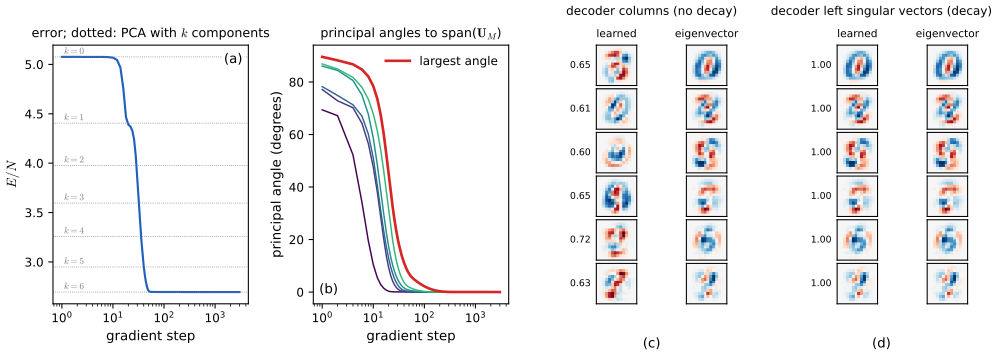
Numerically, Ky Fan's bound holds on 300 random projections, the invariance under \(\bC\) holds to \(10^{-12}\), and gradient descent on 500 centred digits (\(D=196\), \(M=6\)) reaches the PCA error 2.695380 per digit with every principal angle below \(0.001^\circ\), while each decoder column has a cosine of only 0.60–0.72 with its closest eigenvector.
The book adds that "the error function has a unique global minimum". As the result shows, this is true of the map \(\bW_2\bW_1\) (when \(\lambda_M>\lambda_{M+1}\)) but not of the weights, which form an \(M^2\)-dimensional manifold of minimisers. Baldi and Hornik (1989) also showed that every other critical point is a saddle: projections onto any other set of \(M\) eigenvectors make the gradient vanish, and none is a local minimum, which is why gradient descent reaches the global minimum from almost every start.
Filling the gap 19.1: what gradient descent actually finds, plateaus, and how weight decay recovers the eigenvectors p. 565
Result 19.1 describes the set of minimisers; which one training reaches depends on the dynamics. Three facts explain Figure 19.S1 and the demo.
Derivation
A conserved quantity. With \[ E/N=\frac12\Tr((\bI-\bW_2\bW_1)\bS(\bI-\bW_2\bW_1)^\T) \] and \(\bR=(\bW_2\bW_1-\bI)\bS\), the gradients are \(\nabla_{\bW_2}=\bR\bW_1^\T\) and \(\nabla_{\bW_1}=\bW_2^\T\bR\). Under the gradient flow \(\dot\bW=-\nabla\), \[ \frac{\d}{\d t}\big(\bW_1\bW_1^\T-\bW_2^\T\bW_2\big)=-\bW_2^\T\bR\bW_1^\T-\bW_1\bR^\T\bW_2+\bW_1\bR^\T\bW_2+\bW_2^\T\bR\bW_1^\T=\bzero , \] since \(\bR\) is the derivative of a function of \(\bW_2\bW_1\) only. So \(\bW_1\bW_1^\T-\bW_2^\T\bW_2\) is constant (up to \(O(\eta)\) per step for gradient descent). From a small initialisation it is about \(\bzero\): the network stays balanced, \(\bW_1\approx\bW_2^\T\). At the minimum, \(\bW_2=\bU_M\bC\) and \(\bW_1=\bC^{-1}\bU_M^\T\) then force \(\bC^{-\T}\bC^{-1}=\bC^\T\bC\), i.e. \(\bC\) orthogonal: the decoder columns are an orthonormal basis of the principal subspace, but a rotated one. Balance removes the scaling freedom, not the rotation.
Plateaus. \(\bW_1=\bW_2=\bzero\) is a critical point (the gradients are products containing a zero factor). Near it the dynamics are linear: in the eigenbasis, the component of balanced weights along \(\bu_j\) grows like \(e^{\lambda_jt}\), so directions are picked up one after the other, fastest for the largest eigenvalue, after a time of order \(\lambda_j^{-1}\ln(1/\text{scale})\). (Saxe, McClelland and Ganguli, 2014). The loss shows steps where it passes near the saddle points of Baldi and Hornik (projections onto the top \(k<M\) eigenvectors): Figure 19.S1(a) and preset 5 of the demo, where the plateau lengthens as the initial scale shrinks.
Weight decay picks out the eigenvectors. Add \(\frac\mu2(\|\bW_1\|_F^2+\|\bW_2\|_F^2)\). For a given product \(\bA=\bW_2\bW_1\), the smallest penalty over factorisations is \(\mu\sum_k s_k(\bA)\) (the nuclear norm: by the arithmetic-geometric mean inequality \(\|\bW_1\|_F^2+\|\bW_2\|_F^2\ge2\|\bW_2\bW_1\|_*\), with equality for balanced factors). With \(\bA\) restricted to the form \(\sum_ja_j\bu_j\bu_j^\T\) the objective separates: \(\sum_j\big[\frac12\lambda_j(1-a_j)^2+\mu a_j\big]\), minimised at \[ a_j=\Big(1-\frac{\mu}{\lambda_j}\Big)_+ . \] Because the \(a_j\) differ when the \(\lambda_j\) differ, the singular value decomposition of \(\bW_2=\bU_M\diag(\sqrt{a_j})\bC\) (with \(\bC\) orthogonal) is unique up to signs: its left singular vectors are the eigenvectors. The rotation \(\bC\) remains, so the decoder columns are still mixtures, but an SVD of \(\bW_2\) recovers \(\bu_1,\dots,\bu_M\) and their order. (That this diagonal form is the global optimum follows from von Neumann's trace inequality; see Kunin et al., 2019.) Numerically, with \(\mu=0.002\), the cosines are above 0.9999 between the left singular vectors and the eigenvectors, the squared singular values equal \(1-\mu/\lambda_j\) to \(2\times10^{-3}\), and \(\max|\bW_1-\bW_2^\T|=5\times10^{-4}\) (balance). ∎
p. 565 Could nonlinear hidden units escape the linear subspace? Not with linear outputs.
Result 19.2 (nonlinear hidden units with linear outputs cannot beat PCA; Bourlard and Kamp, 1988) p. 565, Figure 19.1
If \(\by=\bW_2\mathbf h(\bx)+\bb_2\) with any hidden map \(\mathbf h:\R^D\to\R^M\), then \(E\ge\frac N2\sum_{j>M}\lambda_j\). With sigmoidal hidden units the bound is approached (by weights so small that the units are nearly linear) but in general not attained.
Proof (short; the full argument is Result 12.17 of the companion course)
Every output lies in the affine set \(\{\bW_2\mathbf h+\bb_2\}\) of dimension at most \(M\), so \(E\) is at least half the summed squared distances of the data to an \(M\)-dimensional affine subspace, which is minimised by PCA (Result 19.1). For approachability: with \(\sigma(a)=\sigma(0)+\sigma'(0)a+O(a^2)\), take hidden pre-activations \(\epsilon\bW_1^\star\bx\) and output weights \(\bW_2^\star/(\epsilon\sigma'(0))\) with a bias absorbing \(\sigma(0)\); the outputs differ from the optimal linear ones by \(O(\epsilon)\), so \(E\to E_{\rm PCA}\) as \(\epsilon\to0\). Equality would need an exactly affine \(\mathbf h\) on the data, which a sigmoid is not, except in degenerate cases. ∎
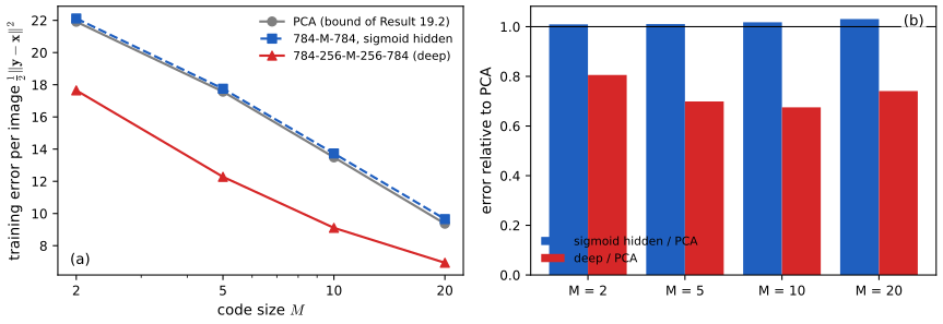
Figure 19.S2(a) confirms both parts: a 784-\(M\)-784 network with sigmoid hidden units stays 0.9–3.1% above the PCA error for \(M=2,5,10,20\).
The book's caption of Figure 19.1 calls such a network "equivalent to linear PCA"; Result 19.2 is the precise version: it is never better, and only asymptotically as good. So there is no reason to train a two-layer network for dimensionality reduction: the singular value decomposition gives the exact answer in finite time, with ordered eigenvalues and orthonormal eigenvectors.
19.1.2 Deep autoencoders
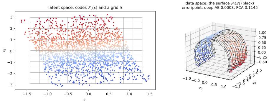
pp. 565–566 The picture changes with more layers. In the four-layer network of Figure 19.2 (a diagram), the first and third layers are sigmoidal and the \(M\) units of the second layer and the outputs are linear. The first half computes a general map \(F_1:\R^D\to\R^M\), the second a general map \(F_2:\R^M\to\R^D\), and \(F_2\) embeds an \(M\)-dimensional surface \(S\) in data space that may be curved (Figure 19.3). This is a nonlinear PCA; training is now a non-convex optimisation with possible poor local minima, and \(M\) must be fixed in advance.
Filling the gap 19.2: "contains PCA as a special case", and when it does better pp. 565–566
Derivation
Containment. With all sigmoidal pre-activations scaled by a small \(\epsilon\) and the following weights by \(1/\epsilon\) (as in the proof of Result 19.2), each sigmoidal layer acts as an affine map up to \(O(\epsilon)\), so the deep network approximates any linear autoencoder, in particular PCA, arbitrarily well. Its infimal error is therefore at most the PCA error.
Strict improvement. For data on a closed curve in the plane, e.g. the unit circle, with \(M=1\): PCA keeps one direction and loses the variance \(\frac12\) of the other, error \(\frac14\) per point. A deep autoencoder can encode the angle \(\theta\) through \(F_1(\bx)=\mathrm{atan2}(x_2,x_1)\) and decode \(F_2(\theta)=(\cos\theta,\sin\theta)\), error zero, apart from the cut where \(F_1\) must jump (a continuous \(F_1\) from the circle to \(\R\) cannot be injective, so a network achieves error approaching zero, not zero). For the bent sheet of Figure 19.3 the trained network's error is 0.0003 per point against 0.1145 for 2-component PCA; on MNIST (Figure 19.S2) the deep autoencoder's error is 68–81% of PCA's. ∎
19.1.3 Sparse autoencoders
See also Section 9.2.2 of these notes, generalized weight decay (why the L1 norm produces exact zeros).
pp. 566–567 Instead of a narrow layer, a penalty can make the code sparse, lowering its effective dimension. With the L1 norm on the activations \(z_k\) of a chosen hidden layer,
\[ \widetilde E(\bw)=E(\bw)+\lambda\sum_{k=1}^K|z_k|, \tag{19.2} \]where, unusually, the regulariser acts on unit activations rather than weights; the gradients come from automatic differentiation.
Filling the gap 19.3: the penalty (19.2) is void unless the decoder's scale is fixed p. 567, (19.2)
The book's (19.2) omits a point that matters in practice: the L1 penalty can be made arbitrarily small without changing a single reconstruction.
Derivation
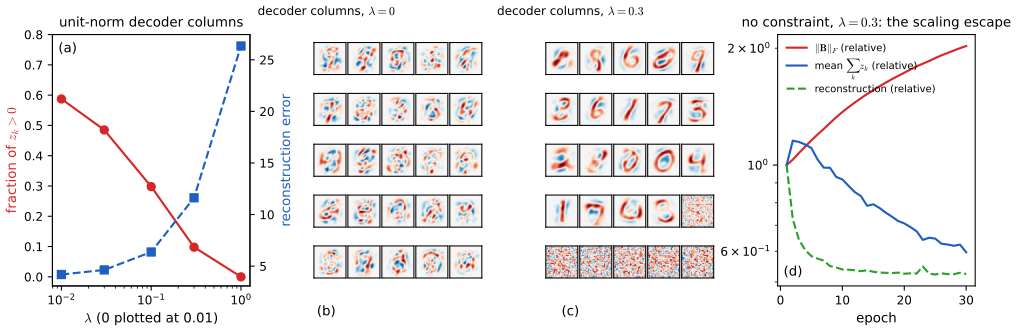
The scaling escape. Suppose the code feeds the decoder linearly, \(\by=\bB\bz+\bb\) (or through a first layer that is linear in \(\bz\)), and the code is \(\bz=\mathrm{ReLU}(\bA\bx+\mathbf a)\) or any positively homogeneous activation. For \(c>0\), replacing \((\bA,\mathbf a,\bB)\) by \((c\bA,c\mathbf a,\bB/c)\) multiplies \(\bz\) by \(c\) and leaves \(\bB\bz\), hence \(E\), unchanged, while the penalty becomes \(c\lambda\sum_k|z_k|\). Letting \(c\to0\) gives \(\inf\widetilde E=\inf E\): at the infimum the penalty has no effect at all. Gradient descent follows this direction: in Figure 19.S3(d), with \(\lambda=0.3\) and no constraint, \(\|\bB\|_F\) doubles in 30 epochs while the code's total activation halves.
Remedies. (i) Fix the decoder scale: renormalise each column of \(\bB\) to unit length after every step (as in sparse coding). (ii) Add weight decay \(\frac\mu2\|\bB\|_F^2\): optimising the scale \(c\) of a fixed solution, \(\lambda cS+\frac{\mu}{2c^2}\|\bB\|^2\) is minimised at \(c^3=\mu\|\bB\|^2/(\lambda S)\), giving a penalty proportional to \((\lambda S)^{2/3}(\mu\|\bB\|^2)^{1/3}\), which is again scale-free and genuinely penalises activity. (iii) Penalise a saturating quantity, e.g. a KL divergence between the mean activation of sigmoid units and a small target rate.
Why zeros appear. For a single activation, the proximal step \(\min_z\frac12(z-a)^2+\lambda|z|\) has the solution \(\sgn(a)\max(|a|-\lambda,0)\) (soft thresholding; the subgradient of \(|z|\) at 0 is \([-1,1]\), so \(z=0\) is optimal whenever \(|a|\le\lambda\)). With ReLU codes the penalty's gradient \(\lambda\) on every active unit pushes pre-activations below zero, where they stay exactly zero. In Figure 19.S3(a), with unit-norm columns, the fraction of active units falls from 0.59 (\(\lambda=0\)) to 0.10 (\(\lambda=0.3\)) and 0 (\(\lambda=1\)), while the reconstruction error rises from 4.2 to 11.6 and 26.3. ∎
19.1.4 Denoising autoencoders
See also the companion course, Section 5.5.5 (training with transformed data) and diffusion models; and Section 14.3 of these notes, Langevin dynamics, which samples with the score.
p. 567 A different way to rule out the identity is to make the network undo a corruption (Vincent et al., 2008). Each \(\bx_n\) is corrupted to \(\xt_n\), and the network is trained to recover the clean input,
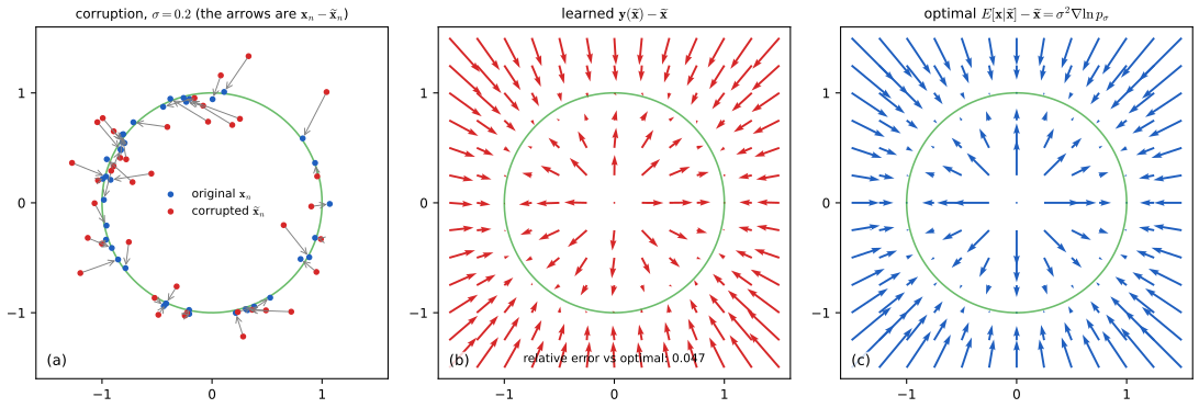
\[ E(\bw)=\sum_{n=1}^N\|\by(\xt_n,\bw)-\bx_n\|^2. \tag{19.3} \]The corruption may set a random fraction \(\nu\in[0,1]\) of the inputs to zero, or add zero-mean Gaussian noise of variance \(\sigma^2\) to every input. To denoise images the network must learn, for example, that neighbouring pixels are correlated. The book then relates the method to score matching (Vincent, 2011), with score \(\bs(\bx)=\nabla_\bx\ln p(\bx)\): the network learns to reverse the displacement \(\xt_n-\bx_n\), a vector pointing back towards the data manifold, as does the score (Figure 19.4). The next result makes this exact.
Result 19.4 (the optimal denoiser, Tweedie's formula and the score) p. 567, (19.3), Figure 19.4
Let \(\bx\sim p\), \(\xt=\bx+\sigma\beps\) with \(\beps\sim\N(\bzero,\bI)\) independent, and \(p_\sigma(\xt)=\int\N(\xt\given\bx,\sigma^2\bI)p(\bx)\,\d\bx\) the density of corrupted data.
- Over all functions, \(\E\|\by(\xt)-\bx\|^2\) is minimised by the posterior mean \(\by^\star(\xt)=\E[\bx\given\xt]\), and the minimum is \(\E\Tr\cov[\bx\given\xt]\).
- (Tweedie's formula.) For every \(\sigma>0\), exactly, \[ \E[\bx\given\xt]-\xt=\sigma^2\nabla_{\xt}\ln p_\sigma(\xt). \]
- (Small noise.) If \(p\) is three times differentiable with bounded derivatives and positive, then \(\nabla\ln p_\sigma=\nabla\ln p+O(\sigma^2)\), so the residual of the optimal denoiser divided by \(\sigma^2\) tends to the score of the data density: \(\big(\by^\star(\xt)-\xt\big)/\sigma^2\to\bs(\xt)\).
Proof
(1) Condition on \(\xt\): \[ \E[\|\by(\xt)-\bx\|^2\given\xt]=\|\by(\xt)-\E[\bx\given\xt]\|^2+\E[\|\bx-\E[\bx\given\xt]\|^2\given\xt] \], because the cross term has conditional mean zero. Only the first term depends on \(\by\), and it vanishes for \(\by=\E[\bx\given\xt]\). A network trained on (19.3) with enough data and capacity therefore approximates the posterior mean (the empirical (19.3) estimates this expectation; with each \(\bx_n\) corrupted afresh at every epoch, it is a stochastic gradient of it).
(2) Differentiate under the integral (allowed since the Gaussian and its gradient are bounded by integrable functions of \(\bx\) uniformly for \(\xt\) in a compact set): \(\nabla_{\xt}\N(\xt\given\bx,\sigma^2\bI)=\frac{\bx-\xt}{\sigma^2}\N(\xt\given\bx,\sigma^2\bI)\), so \[ \nabla p_\sigma(\xt)=\frac1{\sigma^2}\int(\bx-\xt)\N(\xt\given\bx,\sigma^2\bI)p(\bx)\,\d\bx=\frac{p_\sigma(\xt)}{\sigma^2}\big(\E[\bx\given\xt]-\xt\big), \] using Bayes' theorem \(p(\bx\given\xt)=\N(\xt\given\bx,\sigma^2\bI)p(\bx)/p_\sigma(\xt)\). Divide by \(p_\sigma\).
(3) \(p_\sigma=p*\N(\bzero,\sigma^2\bI)\) solves the heat equation \(\partial_tp=\frac12\Delta p\) at time \(t=\sigma^2\), and Taylor's theorem with the moments \(\E\epsilon_i=0\), \(\E\epsilon_i\epsilon_j=\delta_{ij}\), \(\E\epsilon_i\epsilon_j\epsilon_k=0\) gives \(p_\sigma=p+\frac{\sigma^2}2\Delta p+O(\sigma^4)\), and the same for the gradient. Hence \[ \nabla\ln p_\sigma=\frac{\nabla p+\frac{\sigma^2}2\nabla\Delta p}{p+\frac{\sigma^2}2\Delta p}+O(\sigma^4)=\nabla\ln p+O(\sigma^2) \] wherever \(p\) is bounded away from zero. ∎
For the data of Figure 19.4 (an equal mixture of \(\N(\bc_k,\tau^2\bI)\) along a circle, \(\tau=0.03\)) everything is explicit: \(p_\sigma\) is the same mixture with variance \(\tau^2+\sigma^2\) and \(\E[\bx\given\xt]=\sum_kr_k(\xt)\big[\bc_k+\frac{\tau^2}{\tau^2+\sigma^2}(\xt-\bc_k)\big]\) with responsibilities \(r_k\propto\N(\xt\given\bc_k,(\tau^2+\sigma^2)\bI)\). Numerically, (2) agrees with finite differences of \(\ln p_\sigma\) to \(10^{-10}\) and with a Monte Carlo posterior mean, and (3) holds with error \(1.3\times10^{-3}\) at \(\sigma=0.001\), divided by 4 when \(\sigma\) is halved.
Filling the gap 19.4: "points towards the manifold", and what happens at large noise p. 567, Figure 19.4
Figure 19.4 of the book is a sketch; Result 19.4 tells us what the arrows really are, and when the sketch is right.
Derivation
Data on a manifold. Suppose the data lie on a smooth curve (or surface) \(\mathcal M\) and \(\sigma\) is small compared with its curvature radius and with the spacing of any distinct sheets. Given \(\xt\), the likelihood \(\N(\xt\given\bx,\sigma^2\bI)\) is concentrated on the points of \(\mathcal M\) within a few \(\sigma\) of \(\xt\); there \(\mathcal M\) is nearly flat, and \(\|\xt-\bx\|^2=d(\xt)^2+\|\bx-\pi(\xt)\|^2+\dots\), where \(\pi(\xt)\) is the nearest point of \(\mathcal M\) and \(d\) the distance to it. The posterior is then (approximately) a Gaussian of width \(\sigma\) along \(\mathcal M\) centred at \(\pi(\xt)\), so \(\E[\bx\given\xt]\approx\pi(\xt)\): the optimal residual is the vector from \(\xt\) to its projection onto the manifold, orthogonal to \(\mathcal M\). The noise component along \(\mathcal M\) is not undone, since nothing in \(\xt\) reveals it. This is the precise content of the sketch, and Figure 19.4(c) shows it.
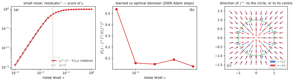
Large noise. When \(\sigma\) is comparable with the size of the data set, the posterior over \(\bx\) spreads over a large part of \(\mathcal M\) and its mean moves inside the convex hull: for the circle, towards the centre (Figure 19.S4(c)). The field is then \(\sigma^2\) times the score of a heavily smoothed density, which no longer points to the nearest data. Diffusion models (Section 20.3 of these notes) train one denoiser for every noise level and chain them.
Score of what? Since \(p\) itself may not have a density (data exactly on \(\mathcal M\)), the DAE estimates the score of \(p_\sigma\), never of \(p\); part (3) of Result 19.4 needs a smooth positive \(p\), and the small-noise limit holds once \(\sigma\ll\tau\) (Figure 19.S4(a), where the relative error behaves like \((\sigma/\tau)^2\)). ∎
Filling the gap 19.5: the denoising loss is score matching (Vincent, 2011) p. 567
The book says that training denoising autoencoders "is related to score matching". Here is the exact relation.
Derivation
Parameterise a score model through the denoiser, \(\bs_\bw(\xt)=(\by(\xt,\bw)-\xt)/\sigma^2\). Two objectives:
Explicit score matching: \(J_{\rm E}(\bw)=\frac12\E_{p_\sigma}\|\bs_\bw(\xt)-\nabla\ln p_\sigma(\xt)\|^2\) (needs the unknown \(p_\sigma\)). Denoising score matching: \[ J_{\rm D}(\bw)=\frac12\E_{p(\bx)\N(\xt\given\bx,\sigma^2\bI)}\|\bs_\bw(\xt)-\nabla_{\xt}\ln\N(\xt\given\bx,\sigma^2\bI)\|^2 \], whose target \((\bx-\xt)/\sigma^2\) is known.
Claim: \(J_{\rm D}(\bw)=J_{\rm E}(\bw)+C\) with \(C\) independent of \(\bw\). Expanding both squares, the terms \(\frac12\E\|\bs_\bw\|^2\) agree, and the terms without \(\bw\) form \(C\). The cross terms agree because, by Tweedie's formula (Result 19.4(2)), \[ \E\Big[\bs_\bw(\xt)^\T\frac{\bx-\xt}{\sigma^2}\Big]=\E\Big[\bs_\bw(\xt)^\T\frac{\E[\bx\given\xt]-\xt}{\sigma^2}\Big]=\E_{p_\sigma}\big[\bs_\bw(\xt)^\T\nabla\ln p_\sigma(\xt)\big]. \] Finally \(\bs_\bw-(\bx-\xt)/\sigma^2=(\by(\xt,\bw)-\bx)/\sigma^2\), so \(J_{\rm D}=\frac1{2\sigma^4}\E\|\by(\xt,\bw)-\bx\|^2\): the expected denoising loss (19.3), scaled. Minimising (19.3) is fitting the score of \(p_\sigma\), without ever evaluating \(p_\sigma\). A Monte Carlo evaluation of \(J_{\rm D}-J_{\rm E}\) for two very different score models gives the same constant (0.04191 and 0.04195). ∎
Result 19.3 (the optimal denoiser for masking noise) p. 567
Let a random mask \(\mathbf m\in\{0,1\}^D\), independent of \(\bx\), zero the entries with \(m_i=0\), and let the network see the corrupted vector together with the mask. The minimiser of \(\E\|\by-\bx\|^2\) copies the visible entries and replaces each hidden entry by its conditional mean given the visible ones: \(y_i^\star=\E[x_i\given\bx_{\rm vis},\mathbf m]\).
Proof
The input is the pair \((\bx_{\rm vis},\mathbf m)\), so by the argument of Result 19.4(1) the optimum is \(\E[\bx\given\bx_{\rm vis},\mathbf m]\). Visible entries are known exactly. For hidden ones, independence of the mask and the data gives \(\E[x_i\given\bx_{\rm vis},\mathbf m]=\E[x_i\given\bx_{\rm vis}]\) for the set of visible indices that \(\mathbf m\) specifies. The network must therefore learn every conditional mean of a subset of pixels given another subset, i.e. the dependence structure of the data, which is the book's point about correlated neighbouring pixels. If the network is not told the mask, a genuine zero and a masked entry are confused and the optimum mixes the two cases; masked autoencoders avoid this by dropping masked tokens and marking positions explicitly. ∎
19.1.5 Masked autoencoders
See also Section 12.3.3 of these notes, encoder transformers (BERT's masked-token training), and Section 12.4.1, vision transformers.
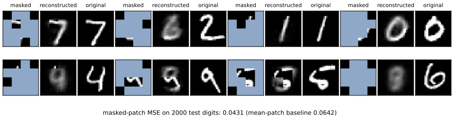
pp. 567–569 BERT learns language representations by predicting masked tokens; the masked autoencoder (He et al., 2021) does the same for images with a vision transformer. The image is cut into patches, a random subset is kept, and only the kept patch tokens enter the encoder (Figure 19.5, an architecture drawing). Images are far more redundant than text (a missing patch rarely changes the meaning, a missing word often does), so the best representations come from masking a large fraction, typically 75% against BERT's 15%; and the masked patches are simply omitted, not replaced by a mask token. The decoder, another transformer, works at full length: the encoder outputs are placed back at their positions, the gaps are filled with one learned mask token, position encodings are added, and a final linear layer predicts pixel values. The loss is the mean squared error over the masked patches only. The decoder is small and is discarded after training; the encoder is then applied to whole, unmasked images and fine-tuned with new output layers.
Result 19.5 (why the loss uses only the masked patches, and how much omission saves) pp. 568–569
(1) With the loss on masked patches only, the optimal decoder output at a masked position is the conditional mean of that patch given the visible patches and their positions. (2) Keeping a fraction \(1-\rho\) of the tokens divides the encoder's attention cost by \((1-\rho)^{-2}\) and its other costs by \((1-\rho)^{-1}\): by 16 and 4 at \(\rho=0.75\).
Proof
The loss. The visible patches enter the encoder, so reconstructing them is trivial (an identity path through the network); including them would spend capacity and gradient on copying. By the argument of Result 19.4(1), minimising the expected squared error on the masked patches makes the decoder output the conditional mean of the hidden patches given the visible ones and their positions: the representation must carry whatever predicts the rest of the image.
The saving. A transformer layer on \(n\) tokens of width \(d\) costs about \(n^2d\) operations for attention and \(nd^2\) for the projections and MLP. Keeping a fraction \(1-\rho\) of the \(N\) patches divides the attention cost by \((1-\rho)^{-2}\) and the rest by \((1-\rho)^{-1}\): at \(\rho=0.75\), by 16 and 4. The decoder runs on all \(N\) tokens, so it is kept narrow and shallow; the book's remark that it "has far fewer learnable parameters" is what keeps the full-length decoder cheap. In the small model of Figure 19.6 (16 patches of \(7\times7\) pixels, 4 visible) the encoder sees 4 tokens instead of 16. ∎
19.2 Variational Autoencoders
See also the companion course, variational autoencoders (Advanced topics, lecture 1), the EM algorithm in general and the evidence decomposition; demos: VAE latent explorer, VAE on Old Faithful, EM lower bound.
pp. 569–570 A deep latent-variable model has the likelihood
\[ p(\bx\given\bw)=\int p(\bx\given\bz,\bw)\,p(\bz)\,\d\bz, \tag{19.4} \]with \(p(\bx\given\bz,\bw)\) defined by a network \(g(\bz,\bw)\) (for example the mean of a Gaussian), which cannot be integrated in closed form. The variational autoencoder (Kingma and Welling, 2013; Rezende, Mohamed and Wierstra, 2014) trains with an approximation built on three ideas: (i) the evidence lower bound, linked to EM; (ii) amortised inference, an encoder network that approximates the posterior for every data point at once; (iii) the reparameterisation trick, which makes the encoder trainable by gradients. The prior is
\[ p(\bz)=\N(\bz\given\bzero,\bI). \tag{19.5} \]Definition 19.2 (variational autoencoder) pp. 570–575, (19.5), (19.13)
A VAE consists of the prior (19.5), a decoder \(p(\bx\given\bz,\bw)\) whose parameters are outputs of a network \(g(\bz,\bw)\), and an encoder \(q(\bz\given\bx,\bphi)=\prod_{j=1}^M\N(z_j\given\mu_j(\bx,\bphi),\sigma_j^2(\bx,\bphi))\) given by a second network. Both are trained jointly by stochastic gradient ascent on \(\sum_n\cL_n(\bw,\bphi)\), the evidence lower bound (19.14), with the expectation estimated through \(\bz=\bmu+\bsig\odot\beps\), \(\beps\sim\N(\bzero,\bI)\). After training, new data are generated by drawing \(\bz\sim p(\bz)\) and decoding.
pp. 570–571 For any distribution \(q(\bz)\),
\[ \ln p(\bx\given\bw)=\cL(\bw)+\KL\big(q(\bz)\|p(\bz\given\bx,\bw)\big), \tag{19.6} \] \[ \cL(\bw)=\int q(\bz)\ln\Big\{\frac{p(\bx\given\bz,\bw)p(\bz)}{q(\bz)}\Big\}\d\bz, \tag{19.7} \] \[ \KL\big(q(\bz)\|p(\bz\given\bx,\bw)\big)=-\int q(\bz)\ln\Big\{\frac{p(\bz\given\bx,\bw)}{q(\bz)}\Big\}\d\bz, \tag{19.8} \]and since \(\KL\ge0\),
\[ \ln p(\bx\given\bw)\ge\cL . \tag{19.9} \]For an i.i.d. data set \(\cD=\{\bx_1,\dots,\bx_N\}\), with a separate latent \(\bz_n\) and distribution \(q_n\) for each point,
\[ \ln p(\cD\given\bw)=\sum_{n=1}^N\cL_n+\sum_{n=1}^N\KL\big(q_n(\bz_n)\|p(\bz_n\given\bx_n,\bw)\big), \tag{19.10} \] \[ \cL_n=\int q_n(\bz_n)\ln\Big\{\frac{p(\bx_n\given\bz_n,\bw)p(\bz_n)}{q_n(\bz_n)}\Big\}\d\bz_n . \tag{19.11} \]Result 19.6 (the evidence decomposition and when the bound is tight) pp. 570–571, (19.6)–(19.12)
(19.6) holds for every density \(q\) with \(q(\bz)>0\Rightarrow p(\bz\given\bx)>0\); \(\cL\le\ln p(\bx)\) with equality if and only if \(q=p(\bz\given\bx,\bw)\) almost everywhere, where
\[ p(\bz_n\given\bx_n,\bw)=\frac{p(\bx_n\given\bz_n,\bw)p(\bz_n)}{p(\bx_n\given\bw)} . \tag{19.12} \]The bound (19.10) is a sum of independent terms, so each \(q_n\) can be optimised separately.
Proof (short; the full argument is Result 10.1 of the companion course)
By the product rule \(p(\bx,\bz)=p(\bz\given\bx)p(\bx)\), so \(\ln\frac{p(\bx\given\bz)p(\bz)}{q(\bz)}=\ln p(\bx)+\ln\frac{p(\bz\given\bx)}{q(\bz)}\). Integrate against \(q\) (which integrates to one): \(\cL=\ln p(\bx)-\KL(q\|p(\bz\given\bx))\), i.e. (19.6). Gibbs' inequality (Result 2.10) gives \(\KL\ge0\) with equality iff the densities agree almost everywhere. For (19.10), \(\ln p(\cD)=\sum_n\ln p(\bx_n)\) by independence; apply (19.6) to each term with its own \(q_n\). ∎
Quadrature confirms (19.6) for the circle model below: \(-4.5401=-8.1846+3.6445\) for a poor Gaussian \(q\), and \(\cL=\ln p\) to \(10^{-8}\) when \(q\) is the exact posterior.
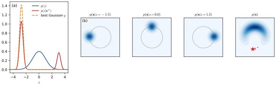
pp. 571–572 For Gaussian mixtures and probabilistic PCA the E step of EM sets each \(q_n\) to the exact posterior, closing the gap (Sections 15.4 and 16.3 of these notes). Here the numerator of (19.12) is easy but the denominator is the intractable likelihood. Figure 19.7 shows why a simple approximation can be poor: for the model of Figure 16.13 (one latent variable, a decoder mean on a circle; Section 16.4.1), a point between the "horns" of the banana-shaped \(p(\bx)\) has a bimodal posterior, although the prior is unimodal.
Filling the gap 19.6: why the posterior is bimodal, and which Gaussian the ELBO prefers p. 572, Figure 19.7
Derivation
Bimodality. \(\ln p(z\given\bx^\star)=-\frac{\|\bx^\star-\bg(z)\|^2}{2\sigma^2}-\frac{z^2}2+\const\) with \[ \|\bx^\star-\bg(z)\|^2=\|\bx^\star\|^2+1-2\|\bx^\star\|\cos(z-\theta^\star) \], where \(\theta^\star\) is the angle of \(\bx^\star\) measured as \(\bg\) does (\(\bx^\star=\|\bx^\star\|(\sin\theta^\star,\cos\theta^\star)\)). The likelihood term is maximal at \(z\in\theta^\star+2\pi\mathbb Z\) with curvature \(\|\bx^\star\|/\sigma^2\), and the prior penalises \(|z|\). For \(\bx^\star=(-0.2,-1.1)\), \(\theta^\star=-2.96\) (close to \(-\pi\)): the candidates \(-2.96\) and \(2\pi-2.96=3.32\) are both within reach of the prior, the second penalised more (\(\frac12z^2\) larger by 1.1), and the strong curvature \(1.12/0.09\approx12\) keeps them separate. The prior pulls each mode towards zero, giving \(-2.74\) and \(3.07\).
Mode seeking. Maximising \(\cL\) over Gaussians is minimising \(\KL(q\|p(z\given\bx))\), which is infinite-penalty-like wherever \(q\) has mass and \(p\) has little: \(q\) avoids the trough between the modes and locks onto one. Each mode is a local optimum (in the demo, starting \(q\) on the right gives the smaller mode and a gap of 1.4 nats instead of 0.30). The companion course derives the best Gaussian in this sense in Result 10.2. ∎
p. 572 A separate model for every \(q_n\), optimised numerically, would be expensive for large data sets and would need re-optimising after every change of \(\bw\). The VAE uses a second network instead.
19.2.1 Amortized inference
pp. 572–574 One encoder network outputs a distribution \(q(\bz\given\bx,\bphi)\) for every input: this is amortised inference, the cost of inference being paid once, in training \(\bphi\), rather than per data point. The ELBO now depends on \(\bphi\) and \(\bw\) and is maximised jointly. The VAE thus has two networks with separate parameters trained together: the encoder, an approximate probabilistic inverse of the decoder by Bayes' theorem, and the decoder. The usual encoder is a diagonal Gaussian,
\[ q(\bz\given\bx,\bphi)=\prod_{j=1}^M\N\big(z_j\given\mu_j(\bx,\bphi),\sigma_j^2(\bx,\bphi)\big), \tag{19.13} \]with linear output units for the means and exponential ones for the variances (so they are positive). Optimisation is joint, by mini-batch stochastic gradients, but one can picture alternating encoder and decoder steps as in EM (Figure 19.8). Unlike the E step of EM, an encoder step does not in general make the KL divergence zero: the true posterior is not a factorised Gaussian, the network has finite flexibility, and training is approximate. Figure 19.9 contrasts the two schemes.
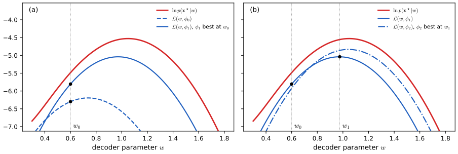
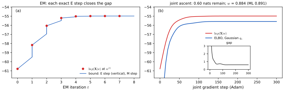
Result 19.7 (what an encoder costs: two gaps, and no monotonicity guarantee) pp. 573–574, Figures 19.8, 19.9
Let \(\mathcal Q\) be the family of factorised Gaussians, \(\cL^\star(\bx)=\max_{q\in\mathcal Q}\cL(q)\), and \(\cL(\bx;\bphi)\) the ELBO of the encoder's \(q(\cdot\given\bx,\bphi)\). Then
\[ \ln p(\bx)-\cL(\bx;\bphi)=\underbrace{\big[\ln p(\bx)-\cL^\star(\bx)\big]}_{\text{approximation gap}\ \ge0}+\underbrace{\big[\cL^\star(\bx)-\cL(\bx;\bphi)\big]}_{\text{amortisation gap}\ \ge0}. \]The first is the KL from the best member of \(\mathcal Q\) to the posterior; the second is the price of predicting \(q\) with one network instead of optimising it per point (Cremer, Li and Duvenaud, 2018). EM with an exact E step increases \(\ln p(\cD\given\bw)\) at every iteration; joint ascent on \(\cL\) increases \(\cL\) (in expectation, for small steps) but not necessarily \(\ln p\), and its maximiser in \(\bw\) is in general not the maximum-likelihood \(\bw\).
Proof
The decomposition is an identity; both brackets are non-negative because \(\cL^\star\) is a maximum over a set containing the encoder's \(q\), and \(\ln p\ge\cL\) for all \(q\) (Result 19.6). For EM, the E step sets \(\cL(q,\bw^{\rm old})=\ln p(\bw^{\rm old})\), the M step raises \(\cL\), and \[ \ln p(\bw^{\rm new})\ge\cL(q,\bw^{\rm new})\ge\cL(q,\bw^{\rm old})=\ln p(\bw^{\rm old}) \] (the companion's Result 9.15). With a gap the first inequality is no longer anchored: \(\cL\) can rise while \(\ln p\) falls, as long as the gap shrinks faster. The maximiser of \(\cL(\bw)=\ln p(\bw)-\mathrm{gap}(\bw)\) satisfies \(\nabla\ln p=\nabla\mathrm{gap}\), which is not zero unless the gap is flat in \(\bw\): the VAE is biased towards decoders whose posteriors are easy to approximate. ∎
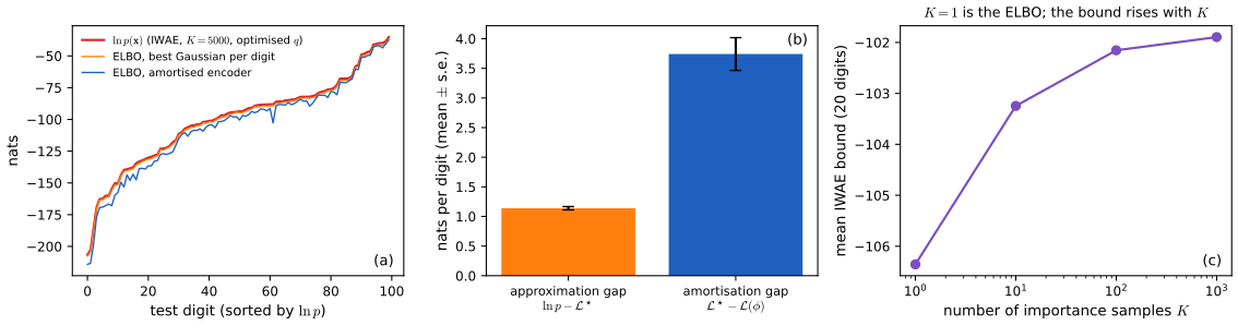
Measured on 100 MNIST test digits with the \(\beta=1\) VAE of Figure 19.S7 (Figure 19.S5): approximation gap 1.14 nats, amortisation gap 3.74 nats per digit; in Figure 19.9(b), \(w=0.884\) against \(w_{\rm ML}=0.891\).
19.2.2 The reparameterization trick
See also Section 14.1.1 of these notes, Filling the gap 14.2 (score-function and reparameterisation estimators, their variances, and when each fails), and its demo.
pp. 574–575 The bound (19.11) still involves an intractable integral over \(\bz_n\). With the encoder it reads
\[ \cL_n(\bw,\bphi)=\int q(\bz_n\given\bx_n,\bphi)\ln\Big\{\frac{p(\bx_n\given\bz_n,\bw)p(\bz_n)}{q(\bz_n\given\bx_n,\bphi)}\Big\}\d\bz_n=\int q(\bz_n\given\bx_n,\bphi)\ln p(\bx_n\given\bz_n,\bw)\,\d\bz_n-\KL\big(q(\bz_n\given\bx_n,\bphi)\|p(\bz_n)\big). \tag{19.14} \]The second term is a KL divergence between two Gaussians, available in closed form. The book prints it (Exercise 2.27) as
\[ \KL\big(q(\bz_n\given\bx_n,\bphi)\|p(\bz_n)\big)\overset{?}{=}\frac12\sum_{j=1}^M\big\{1+\ln\sigma_j^2(\bx_n)-\mu_j^2(\bx_n)-\sigma_j^2(\bx_n)\big\}, \tag{19.15} \]but the right-hand side is minus the divergence: it is \(\le0\) (each brace is \(1+\ln s-s-\mu^2\le0\) since \(\ln s\le s-1\)), whereas a KL divergence is \(\ge0\). The correct statement is Result 19.9; the right-hand side of (19.15) is what is added to the bound, which is how (19.19) and Algorithm 19.1 use it.
Result 19.9 (KL divergence between Gaussians, and its gradients) p. 574, (19.15); Exercises 19.3, 19.4; Exercise 2.27
For \(q=\N(\bmu_1,\Sig_1)\) and \(p=\N(\bmu_2,\Sig_2)\) in \(\R^M\), \[ \KL(q\|p)=\frac12\Big[\Tr(\Sig_2^{-1}\Sig_1)+(\bmu_2-\bmu_1)^\T\Sig_2^{-1}(\bmu_2-\bmu_1)-M+\ln\frac{\det\Sig_2}{\det\Sig_1}\Big]. \] For the encoder (19.13) against \(\N(\bzero,\bI)\): \[ \KL=\frac12\sum_{j=1}^M\big(\mu_j^2+\sigma_j^2-1-\ln\sigma_j^2\big),\qquad\frac{\partial\KL}{\partial\mu_j}=\mu_j,\qquad\frac{\partial\KL}{\partial\ln\sigma_j^2}=\frac12(\sigma_j^2-1). \] For a full covariance \(\Sig=\bL\bL^\T\) (Exercise 19.3), \(\KL=\frac12\big(\Tr\bL\bL^\T+\bmu^\T\bmu-M-2\sum_j\ln L_{jj}\big)\).
Proof
\(\KL(q\|p)=\E_q[\ln q-\ln p]\) with \[ \ln\N(\bz\given\bmu,\Sig)=-\frac M2\ln2\pi-\frac12\ln\det\Sig-\frac12(\bz-\bmu)^\T\Sig^{-1}(\bz-\bmu) \]. Under \(q\), \(\E[(\bz-\bmu_1)^\T\Sig_1^{-1}(\bz-\bmu_1)]=\Tr(\Sig_1^{-1}\Sig_1)=M\), and, writing \(\bz-\bmu_2=(\bz-\bmu_1)+(\bmu_1-\bmu_2)\) and using \(\E[\bz-\bmu_1]=\bzero\), \[ \E[(\bz-\bmu_2)^\T\Sig_2^{-1}(\bz-\bmu_2)]=\Tr(\Sig_2^{-1}\Sig_1)+(\bmu_1-\bmu_2)^\T\Sig_2^{-1}(\bmu_1-\bmu_2) \]. Subtracting gives the formula. With \(\bmu_2=\bzero\), \(\Sig_2=\bI\), \(\Sig_1=\diag(\sigma_j^2)\): \(\Tr\Sig_1=\sum\sigma_j^2\), \(\ln\det\Sig_1=\sum\ln\sigma_j^2\). The derivatives follow term by term (\(\partial\sigma^2/\partial\ln\sigma^2=\sigma^2\)). For \(\Sig=\bL\bL^\T\) with \(\bL\) triangular, \(\det\Sig=(\det\bL)^2=\prod_jL_{jj}^2\). Each summand \(\frac12(\mu^2+s-1-\ln s)\) is \(\ge0\), zero only at \(\mu=0\), \(s=1\). ∎
Numerically: the diagonal formula against Monte Carlo (1.6057 against 1.6066; the printed (19.15) gives \(-1.6057\)), the gradients against automatic differentiation to \(10^{-12}\), and the full-covariance formula against Monte Carlo (6.8332 against 6.8338).
p. 575 For the first term of (19.14) one could average over samples from the encoder,
\[ \int q(\bz_n\given\bx_n,\bphi)\ln p(\bx_n\given\bz_n,\bw)\,\d\bz_n\simeq\frac1L\sum_{l=1}^L\ln p(\bx_n\given\bz_n^{(l)},\bw), \tag{19.16} \]which is easy to differentiate in \(\bw\) but not in \(\bphi\): \(\bphi\) changes the distribution the samples come from, while each sample is a fixed number (Figure 19.10, a diagram: sampling blocks backpropagation). The reparameterisation trick writes the sample as a differentiable function of \(\bphi\) and of noise that does not depend on \(\bphi\). If \(\epsilon\) has zero mean and unit variance and is Gaussian, then
\[ z=\sigma\epsilon+\mu \tag{19.17} \]is Gaussian with mean \(\mu\) and variance \(\sigma^2\) (Exercise 19.2), so the samples of (19.16) can be drawn as \(z_{nj}^{(l)}=\mu_j(\bx_n,\bphi)+\sigma_j(\bx_n,\bphi)\epsilon_{nj}^{(l)}\). The book prints this as
\[ z_{nj}^{(l)}\overset{?}{=}\mu_j(\bx_n,\bphi)\epsilon_{nj}^{(l)}+\sigma_j^2(\bx_n,\bphi), \tag{19.18} \]with mean and variance swapped and the variance where the standard deviation belongs; the text after (19.19) and (19.17) itself give the correct \(\sigma_{nj}\epsilon+\mu_{nj}\). The trick needs continuous variables; gradient estimators without it exist (Williams, 1992; Exercise 19.1) but have high variance, so reparameterisation can also be seen as variance reduction. With the corrected (19.15), the training objective is
\[ \cL=\sum_n\Big\{\frac12\sum_{j=1}^M\big(1+\ln\sigma_{nj}^2-\mu_{nj}^2-\sigma_{nj}^2\big)+\frac1L\sum_{l=1}^L\ln p(\bx_n\given\bz_n^{(l)},\bw)\Big\}, \tag{19.19} \]with \(z_{nj}^{(l)}=\sigma_{nj}\epsilon^{(l)}+\mu_{nj}\), summed over a mini-batch, usually with \(L=1\): one noisy sample adds little to the noise of a mini-batch gradient and is cheaper (Figure 19.11, a diagram, shows the noise entering from the side).
Result 19.8 (the reparameterisation gradient is unbiased) pp. 575–576, (19.16)–(19.19)
Let \(\bz=\bmu(\bphi)+\bsig(\bphi)\odot\beps\), \(\beps\sim\N(\bzero,\bI)\), and let \(f(\bz)\) be differentiable with \(\E\|\nabla f(\bz)\|\) finite and locally uniformly bounded in \(\bphi\). Then \[ \nabla_\bphi\E_{q_\bphi}[f(\bz)]=\E_\beps\Big[\Big(\frac{\partial\bz}{\partial\bphi}\Big)^\T\nabla_\bz f(\bz)\Big],\qquad\frac{\partial}{\partial\mu_j}\E[f]=\E\Big[\frac{\partial f}{\partial z_j}\Big],\quad\frac{\partial}{\partial\ln\sigma_j}\E[f]=\E\Big[\frac{\partial f}{\partial z_j}\sigma_j\epsilon_j\Big], \] so each term of (19.19) (and its \(L=1\) version) is an unbiased estimate of \(\cL_n\) whose gradient, by backpropagation through \(\bz\), is an unbiased estimate of \(\nabla_{\bw,\bphi}\cL_n\).
Proof
\(\E_q[f(\bz)]=\E_\beps[f(\bmu+\bsig\odot\beps)]\) because \(\bmu+\bsig\odot\beps\) has the distribution \(q\) (Exercise 19.2, coordinate by coordinate). The distribution of \(\beps\) does not depend on \(\bphi\), so the derivative passes inside the expectation (dominated convergence, with the assumed bound) and the chain rule gives \(\partial f/\partial\phi=\sum_j\frac{\partial f}{\partial z_j}\big(\frac{\partial\mu_j}{\partial\phi}+\epsilon_j\frac{\partial\sigma_j}{\partial\phi}\big)\). The KL term is differentiated exactly (Result 19.9), and \(\nabla_\bw\) commutes with the expectation over a distribution that does not depend on \(\bw\). ∎
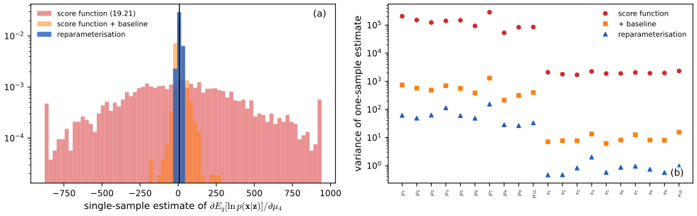
The conditions matter: for a step function \(f\) the formula gives 0 and is wrong (Filling the gap 14.2). The estimator agrees with finite differences of the exact ELBO of the circle model (\(-2.6092\) against \(-2.6088\) for \(\partial/\partial m\)); on MNIST both single-sample estimators are unbiased but the score-function variance is 1100 to 3000 times larger, coordinate by coordinate (Figure 19.S6).
Filling the gap 19.7: what the likelihood term is for Gaussian and Bernoulli decoders pp. 575–578
Derivation
Gaussian decoder \(p(\bx\given\bz,\bw)=\N(\bx\given g(\bz,\bw),s^2\bI)\): \[ \ln p(\bx\given\bz,\bw)=-\frac1{2s^2}\|\bx-g(\bz,\bw)\|^2-\frac D2\ln(2\pi s^2) \]. The ELBO is then minus a squared reconstruction error weighted by \(1/2s^2\), minus the KL: a deterministic autoencoder (19.1) with noise injected into the code and a penalty pulling the codes towards \(\N(\bzero,\bI)\). With \(s\) fixed, it is the size of \(s\) that sets how much reconstruction is worth relative to the KL (Result 19.10). Bernoulli decoder (binary pixels) with means \(\pi_i=\mathrm{sigmoid}(a_i(\bz,\bw))\): \(\ln p=\sum_i[x_i\ln\pi_i+(1-x_i)\ln(1-\pi_i)]\), the negative cross-entropy, used for the MNIST models here (on binarised digits, so that the ELBO is a genuine bound in nats). The book's closing remark (p. 578) that the decoder may also output a variance or other distribution parameters corresponds to mixture density networks (Section 6.5). ∎
Algorithm 19.1 (variational autoencoder training, corrected) p. 577
Input: data \(\{\bx_n\}\), encoder \(\{\mu_j(\bx,\bphi),\sigma_j^2(\bx,\bphi)\}_{j=1}^M\), decoder \(g(\bz,\bw)\), initial \(\bw,\bphi\), learning rate \(\eta\). Repeat until converged, for a data point (in practice a mini-batch) \(\bx_n\):
- \(\cL\leftarrow0\).
- For \(j=1,\dots,M\): draw \(\epsilon_{nj}\sim\N(0,1)\); set \(z_{nj}\leftarrow\mu_j(\bx_n,\bphi)+\sigma_j(\bx_n,\bphi)\,\epsilon_{nj}\) (the book prints \(\mu_j\epsilon_{nj}+\sigma_j^2\)); add \(\frac12(1+\ln\sigma_{nj}^2-\mu_{nj}^2-\sigma_{nj}^2)\), which is \(-\KL\) for this coordinate, to \(\cL\).
- \(\cL\leftarrow\cL+\ln p(\bx_n\given\bz_n,\bw)\).
- \(\bw\leftarrow\bw+\eta\nabla_\bw\cL\), \(\bphi\leftarrow\bphi+\eta\nabla_\bphi\cL\) (ascent: \(\cL\) is maximised), with both gradients by backpropagation through \(\bz_n\).
Return \(\bw,\bphi\). After training, discard the encoder and generate by \(\bz\sim\N(\bzero,\bI)\), \(\bx\sim p(\bx\given\bz,\bw)\).
p. 576 To judge a trained model on a test point \(\widehat\bx\), the book suggests using the bound, estimated with samples from \(q(\bz\given\widehat\bx,\bphi)\) rather than from \(p(\bz)\), as more accurate. Importance weighting makes this precise.
Result 19.12 (the importance-weighted estimate of the test likelihood) p. 576
With \(\bz_1,\dots,\bz_K\) drawn independently from \(q(\bz\given\bx)\) and weights \(w_k=p(\bx\given\bz_k)p(\bz_k)/q(\bz_k\given\bx)\): (1) \(\frac1K\sum_kw_k\) is an unbiased estimate of \(p(\bx)\); (2) \(\cL_K=\E\ln\frac1K\sum_kw_k\le\ln p(\bx)\), \(\cL_1\) is the ELBO, and \(\cL_K\) is non-decreasing in \(K\) (Burda, Grosse and Salakhutdinov, 2016); (3) the variance of (1) is \(\frac1K\big(\int\frac{p(\bx,\bz)^2}{q(\bz)}\d\bz-p(\bx)^2\big)\), zero when \(q\) is the exact posterior, and typically enormous for \(q=p(\bz)\), whose samples rarely fall where \(p(\bx\given\bz)\) is large.
Proof
(1) \(\E_q[w]=\int p(\bx,\bz)\,\d\bz=p(\bx)\). (2) Jensen's inequality for the concave \(\ln\) gives \(\cL_K\le\ln\E[\frac1K\sum w_k]=\ln p(\bx)\). For monotonicity, write the average of \(K+1\) weights as the mean, over the \(K+1\) ways of leaving one out, of averages of \(K\) weights; by concavity \(\ln\) of that mean is at least the mean of the logs, and each of those has expectation \(\cL_K\). (3) The variance of one weight is \(\E_q[w^2]-p(\bx)^2\); if \(q=p(\bz\given\bx)\) then \(w\equiv p(\bx)\). ∎
On 20 MNIST test digits, \(\cL_K\) is \(-106.4\), \(-103.3\), \(-102.2\), \(-101.9\) for \(K=1,10,100,1000\) (Figure 19.S5(c)).
pp. 576–577 Variants: for images, convolutional encoders and transpose-convolution decoders (Section 10.5.3); the conditional VAE, in which encoder and decoder both receive a condition \(\bc\) such as a class label, and the prior may become a network \(p(\bz\given\bc)\). Its bound is the same derivation conditioned on \(\bc\): \[ \ln p(\bx\given\bc)\ge\E_{q(\bz\given\bx,\bc)}[\ln p(\bx\given\bz,\bc)]-\KL(q(\bz\given\bx,\bc)\|p(\bz\given\bc)) \].
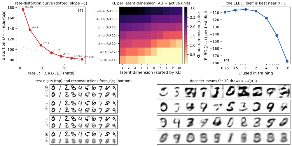
pp. 576–577 The KL term of (19.14) pulls \(q(\bz\given\bx,\bphi)\) towards the prior, which is what makes decoded prior samples realistic. (The book calls this "the first term in the ELBO (19.14)"; it is the second.) Two failure modes follow. In posterior collapse, \(q(\bz\given\bx)\) becomes the prior, the code ignores the input, \(\KL\approx0\), and reconstructions are blurry. In the opposite case, the code is not compressed, reconstructions are excellent, \(\KL\) is large, and samples from the prior are poor because the encoder's distributions are far from \(p(\bz)\). Both can be addressed by a coefficient \(\beta\) on the KL term (the book again says "first term"), typically \(\beta>1\) (Higgins et al., 2017), possibly annealed from a small value during training. The book recommends increasing \(\beta\) when reconstructions look poor and decreasing it when samples look poor; this is reversed. A larger \(\beta\) weights the KL more, lowers the rate and worsens reconstructions (more collapse); poor reconstructions call for a smaller \(\beta\), poor samples for a larger one. Figure 19.S7 shows this directly: the distortion rises monotonically from 81.5 nats at \(\beta=0.25\) to 176.4 at \(\beta=16\).
Result 19.10 (what β is: a Lagrange multiplier, and a decoder variance; Alemi et al., 2018) p. 577
Let \(R(\bphi)=\E_{\bx}\KL(q(\bz\given\bx,\bphi)\|p(\bz))\) (the rate) and \(D(\bw,\bphi)=-\E_\bx\E_q\ln p(\bx\given\bz,\bw)\) (the distortion). Maximising the \(\beta\)-weighted bound means minimising \(D+\beta R\).
- Every solution minimises \(D\) subject to \(R\le R^\star\), its own rate; along the curve of optimal \((R,D)\) pairs, where it is differentiable, \(\d D/\d R=-\beta\). Hence \(\beta\) is the exchange rate between nats of code and nats of reconstruction; at \(\beta=1\), \(-(D+R)\) is the ELBO itself.
- For a Gaussian decoder with fixed variance \(s^2\), the \(\beta\)-weighted bound equals \(\beta\) times the ordinary ELBO of the same model with variance \(\beta s^2\), plus a constant. So \(\beta>1\) is the same as assuming a noisier decoder.
- \(R\ge I_q(\bx;\bz)\), the mutual information between data and code under \(q(\bx,\bz)=p_{\rm data}(\bx)q(\bz\given\bx)\), so \(R\to0\) forces the code to carry no information about \(\bx\).
Proof
(1) If \((\bw,\bphi)\) minimises \(D+\beta R\) and some \((\bw',\bphi')\) had \(R'\le R\), \(D'<D\), then \(D'+\beta R'<D+\beta R\), a contradiction. If \(D^\star(R)\) is the optimal-distortion curve, the minimiser of \(D^\star(R)+\beta R\) over \(R\) satisfies \(D^{\star\prime}(R)=-\beta\). (2) \(\E_q\ln\N(\bx\given g,s^2\bI)=-\frac{\E_q\|\bx-g\|^2}{2s^2}-\frac D2\ln2\pi s^2\), hence \[ \E_q\ln p_{s^2}-\beta\KL=\beta\big[-\frac{\E_q\|\bx-g\|^2}{2\beta s^2}-\KL\big]+\const=\beta\big[\E_q\ln p_{\beta s^2}-\KL\big]+\const' \]. (3) \[ R=\E_\bx\E_q\ln\frac{q(\bz\given\bx)}{p(\bz)}=I_q(\bx;\bz)+\KL(q(\bz)\|p(\bz))\ge I_q \], where \(q(\bz)=\E_\bx q(\bz\given\bx)\) is the aggregate posterior. ∎
Part (3) also explains poor samples at small \(\beta\): the second piece, \(\KL(q(\bz)\|p(\bz))\), measures how far the codes of the data are from the prior that samples are drawn from. Part (2) holds numerically to \(10^{-10}\), and the slope in (1) on the closed-form curve of Result 19.11.
Filling the gap 19.8: why posterior collapse happens pp. 576–577
Derivation
Total collapse is self-consistent. If \(R=0\) then, by Gibbs' inequality, \(q(\bz\given\bx)=p(\bz)\) for almost every \(\bx\): the code is independent of the data, and the best decoder for such codes maximises \(\E_{p(\bz)}\E_\bx\ln p(\bx\given\bz)\), i.e. it models the data marginal alone, the same for every \(\bz\). Conversely, a decoder that ignores \(\bz\) makes the reconstruction term independent of \(q\), and the ELBO is then maximised by \(q=p(\bz)\). So "encoder equals prior, decoder ignores the code" is a stationary configuration, and a local optimum that gradient training can fall into, especially early in training when the decoder is weak, which is why KL annealing (starting from small \(\beta\)) helps.
When it is the global optimum. If the decoder family is rich enough to represent \(p_{\rm data}(\bx)\) without \(\bz\) (e.g. a powerful autoregressive decoder), the collapsed solution attains \(\cL=\E\ln p_{\rm data}\), the largest value any model can have, so nothing is gained by using the code: the ELBO cannot be beaten by informative codes. With limited decoders, information in \(\bz\) is worth its rate only if it reduces the distortion by more (in nats, times \(1/\beta\)). Result 19.11 makes this exact for linear models: a direction of the data is encoded only if its variance exceeds the decoder noise \(\beta s^2\). ∎
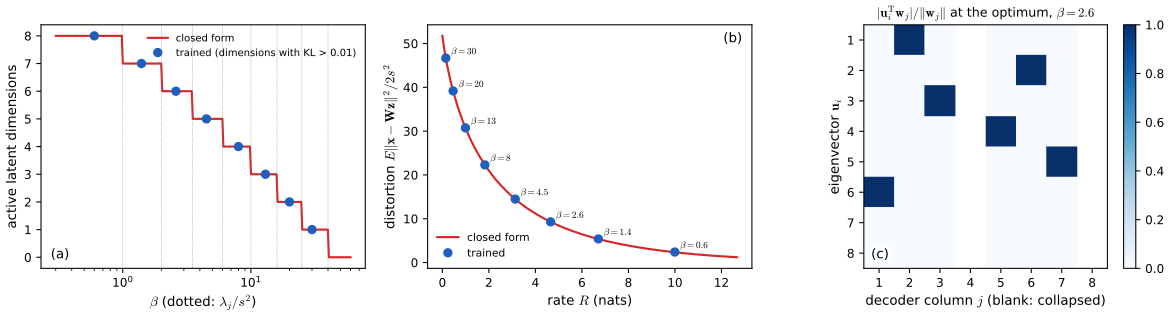
Result 19.11 (the linear Gaussian VAE: collapse and the rate-distortion curve in closed form) supplement to p. 577
Let the data have covariance with eigenvalues \(\lambda_1>\dots>\lambda_D\) and eigenvectors \(\bu_j\); take \(p(\bz)=\N(\bzero,\bI_M)\), \(p(\bx\given\bz)=\N(\bW\bz+\bb,s^2\bI)\) with \(s^2\) fixed, and a linear encoder \(q(\bz\given\bx)=\N(\bV\bx+\bc,\diag(\bsig^2))\). Maximise \(\E_\bx[\E_q\ln p(\bx\given\bz)-\beta\KL]\), and set \(\theta=\beta s^2\). At the optimum:
- direction \(j\le M\) is active if and only if \(\lambda_j>\theta\); otherwise its latent dimension collapses to the prior (\(\KL_j=0\), decoder column zero);
- \(R=\sum_{j\le M}\frac12\ln\frac{\lambda_j}{\theta}\Big|_+\) and \[ \E\|\bx-\bW\bz-\bb\|^2=\sum_{j\le M}\min(\lambda_j,\theta)+\sum_{j>M}\lambda_j \]: reverse water-filling at level \(\theta\), the rate-distortion function of a Gaussian source; along the curve \(\d D/\d R=-\beta\) with \(D\) in nats (squared error over \(2s^2\));
- the active decoder columns are, up to sign and order, \(\sqrt{\lambda_j-\theta}\,\bu_j\): unlike the deterministic linear autoencoder (Result 19.1), the diagonal-covariance encoder identifies the eigenvectors.
Proof
By Result 19.10(2) the objective is \(\beta\) times the ELBO of probabilistic PCA with noise variance \(\theta\), plus a constant. For a linear-Gaussian model the exact posterior is Gaussian, \(\N\big(\bM^{-1}\bW^\T(\bx-\bb),\theta\bM^{-1}\big)\) with \(\bM=\bW^\T\bW+\theta\bI\), and an encoder of the stated form can equal it whenever \(\bM\) is diagonal; then the ELBO equals the log likelihood. The maximum-likelihood solution of probabilistic PCA (Tipping and Bishop, 1999; the companion's Result 12.8) is \(\bW=\bU_M(\bLam_M-\theta\bI)_+^{1/2}\bR\) with \(\bR\) orthogonal, and \(\bM=\bR^\T\diag(\max(\lambda_j,\theta))\bR\) is diagonal for \(\bR=\bI\) (up to signed permutations). So the ELBO's maximum equals the likelihood's maximum and is attained by \(\bW=\bU_M(\bLam_M-\theta)_+^{1/2}\) with a matching encoder. For any other \(\bR\), \(\bM\) is not diagonal (when the active \(\lambda_j\) are distinct), the diagonal \(q\) cannot equal the posterior, and the ELBO is strictly smaller: the diagonal constraint breaks the rotation symmetry (Lucas et al., 2019). This gives (1) and (3).
(2) In coordinates \(a_j=\bu_j^\T(\bx-\bar\bx)\), \(\var a_j=\lambda_j\). For an active \(j\), \(w_j^2=\lambda_j-\theta\), the posterior variance is \(v_j=\theta/(w_j^2+\theta)=\theta/\lambda_j\) and the mean \(m_j=w_ja_j/\lambda_j\), with \(\E m_j^2=w_j^2/\lambda_j\). Then \[ \KL_j=\frac12(\E m_j^2+v_j-1-\ln v_j)=\frac12\big(\frac{\lambda_j-\theta}{\lambda_j}+\frac\theta{\lambda_j}-1+\ln\frac{\lambda_j}\theta\big)=\frac12\ln\frac{\lambda_j}\theta \], and the expected squared error along \(\bu_j\) is \[ \E(a_j-w_jm_j)^2+w_j^2v_j=\lambda_j\frac{\theta^2}{\lambda_j^2}+(\lambda_j-\theta)\frac{\theta}{\lambda_j}=\theta \]. Inactive directions cost \(\lambda_j\) and no rate. With \(k\) active directions, \(\d R/\d\theta=-k/2\theta\) and \(\d(\sum\min)/\d\theta=k\), so \(\d(\text{squared error})/\d R=-2\theta\) and, dividing by \(2s^2\), \(\d D/\d R=-\beta\), as Result 19.10(1) requires. ∎
Numerically: the optimum found by L-BFGS on the closed-form objective matches (1)–(2) to \(6\times10^{-8}\) and its active columns have cosine above 0.999 with eigenvectors; VAEs trained by reparameterised stochastic gradients land within 1% of the closed-form curve (Figure 19.S8).
Summary: errors and imprecisions found in the chapter (first printing)
- (19.15): the right-hand side is \(-\KL\), not \(\KL\): each term \(1+\ln\sigma^2-\mu^2-\sigma^2\le0\). The correct formula is \(\frac12\sum_j(\mu_j^2+\sigma_j^2-1-\ln\sigma_j^2)\) (Result 19.9; numerically: closed form 1.6057, Monte Carlo 1.6066, printed expression \(-1.6057\)). (19.19) and Algorithm 19.1 add the printed expression to the bound, which is correct.
- (19.18) and Algorithm 19.1: \(z_{nj}=\mu_j\epsilon_{nj}+\sigma_j^2\) should be \(z_{nj}=\mu_j+\sigma_j\epsilon_{nj}\), as in (19.17) and the text after (19.19). As printed, the sample would have mean \(\sigma_j^2\) and standard deviation \(|\mu_j|\).
- pp. 576–577: "the first term in the ELBO (19.14) encourages the encoder distribution to be close to the prior" and "a coefficient \(\beta\) in front of the first term in (19.14)": both refer to the KL divergence, the second term of (19.14).
- p. 577, the advice on \(\beta\) is reversed: poor reconstructions (collapse) call for decreasing \(\beta\), poor samples for increasing it. Evidence: on MNIST the distortion rises monotonically with \(\beta\), from 81.5 nats (\(\beta=0.25\)) to 176.4 (\(\beta=16\)), and the number of active latent dimensions falls from 10 to 4 (Figure 19.S7); in closed form, a direction collapses exactly when \(\beta\) exceeds \(\lambda_j/s^2\) (Result 19.11).
- Exercise 19.1: the Monte Carlo estimator (19.21) needs a factor \(1/S\) (with \(S\) the number of samples) to be unbiased; "\(G(\bz)=p(\bx\given\bz,\bw)\)" should be \(\ln p(\bx\given\bz,\bw)\); and that is the first term on the right of (19.14), not the second.
- Exercise 19.3: \(\beps\sim\N(\bz\given\bzero,\bI)\) should read \(\N(\beps\given\bzero,\bI)\); and the diagonal of \(\bL\) must be strictly positive (not merely non-negative) for \(\Sig\) to be non-singular and the factor unique (solution).
- p. 564 (imprecision): with linear hidden units the error has a unique global minimum as a map \(\bW_2\bW_1\) (when \(\lambda_M>\lambda_{M+1}\)), but not in the weights, which are determined only up to an invertible \(M\times M\) matrix (Result 19.1). Likewise the caption of Figure 19.1 ("equivalent to linear PCA" with nonlinear hidden units): such a network can never beat PCA and reaches it only in a limit (Result 19.2).
- p. 567 (omission): the L1 activation penalty (19.2) can be driven to zero by rescaling the encoder and decoder without changing any reconstruction, unless the decoder's scale is constrained (Filling the gap 19.3; observed in training, Figure 19.S3(d)).
Exercises
All 6 exercises of Chapter 19 (Bishop and Bishop, 2024, pp. 578–579), restated in my own words, with complete solutions (hidden). Stars give the book's difficulty. The official solutions manual stops at Chapter 10, so these solutions are my own.
Exercise 19.1 (★★). For a distribution \(q(\bz\given\bphi)\) and a function \(G(\bz)\), show that
\[ \nabla_\bphi\int q(\bz\given\bphi)G(\bz)\,\d\bz=\int q(\bz\given\bphi)G(\bz)\nabla_\bphi\ln q(\bz\given\bphi)\,\d\bz, \tag{19.20} \]so that the left side can be estimated from independent samples \(\bz^{(i)}\sim q(\bz\given\bphi)\) by
\[ \nabla_\bphi\int q(\bz\given\bphi)G(\bz)\,\d\bz\simeq\sum_iG(\bz^{(i)})\nabla_\bphi\ln q(\bz^{(i)}\given\bphi), \tag{19.21} \]and show the estimator is unbiased. Discuss its use for the encoder gradient of the reconstruction term of (19.14) without the reparameterisation trick.
Solution
Identity. Assume \(q\) is differentiable in \(\bphi\), its support does not depend on \(\bphi\), and \(|G\,\nabla_\bphi q|\) is dominated by an integrable function near the current \(\bphi\), so that differentiation and integration commute. Then \(\nabla_\bphi\int qG=\int G\nabla_\bphi q=\int qG\nabla_\bphi\ln q\), since \(\nabla q=q\nabla\ln q\) wherever \(q>0\).
Estimator. (19.20) is an expectation under \(q\), so for \(S\) independent samples \(\widehat\bg=\frac1S\sum_{i=1}^SG(\bz^{(i)})\nabla_\bphi\ln q(\bz^{(i)}\given\bphi)\) has \(\E\widehat\bg=\frac1S\cdot S\cdot\E_q[G\nabla\ln q]\), the left side of (19.20): unbiased. As printed, without the \(1/S\), (19.21) has expectation \(S\) times the gradient. Its variance is \(\frac1S\cov_q[G\nabla\ln q]\), so the error vanishes as \(S\to\infty\), as the book says. Two remarks: since \(\E_q[\nabla_\bphi\ln q]=\nabla_\bphi\int q=\bzero\), any constant baseline \(b\) can be subtracted from \(G\) without bias, which often reduces the variance a lot; and for the VAE the function is \(G(\bz)=\ln p(\bx\given\bz,\bw)\) (not \(p\)), the first term of (19.14).
Why reparameterisation is preferred. The score-function estimator uses only values of \(G\), not its gradient, so it does not "see" how \(G\) changes when \(\bz\) moves; its variance grows with the size of \(G\) (here hundreds of nats). For one MNIST digit, Figure 19.S6 shows single-sample variances 1100 to 3000 times larger than with reparameterisation, coordinate by coordinate, and a baseline closes only part of the gap. It remains essential when \(G\) is not differentiable or \(\bz\) is discrete (Filling the gap 14.2). Numerically: with \(S=50\), \(G=\sin3z+z^2\), \(q=\N(0.7,0.4^2)\), the mean of 4000 estimates is 0.6648 against the exact 0.6628.
Exercise 19.2 (★). If \(\epsilon\sim\N(0,1)\), show that \(z=\sigma\epsilon+\mu\) in (19.17) is \(\N(\mu,\sigma^2)\).
Solution
For \(\sigma>0\) the map is increasing with inverse \(\epsilon=(z-\mu)/\sigma\) and \(\d\epsilon/\d z=1/\sigma\), so by the change of variables formula \[ p(z)=\N\big(\frac{z-\mu}\sigma\given0,1\big)\frac1\sigma=\frac1{\sqrt{2\pi\sigma^2}}\exp\big(-\frac{(z-\mu)^2}{2\sigma^2}\big)=\N(z\given\mu,\sigma^2) \]. (For \(\sigma<0\) use \(|\d\epsilon/\d z|=1/|\sigma|\) and the symmetry of \(\N(0,1)\): the result is \(\N(\mu,\sigma^2)\) again.) Directly: \(\E z=\sigma\E\epsilon+\mu=\mu\), \(\var z=\sigma^2\var\epsilon=\sigma^2\), and an affine function of a Gaussian is Gaussian. Confirmed on 400 000 draws (mean, variance, Kolmogorov–Smirnov).
Exercise 19.3 (★★). For a full-covariance encoder, let
\[ \beps\sim\N(\beps\given\bzero,\bI_K), \tag{19.22} \] \[ \bz=\bmu+\bL\beps \tag{19.23} \]with \(\bL\) a \(K\times K\) lower-triangular matrix. Show that \(\bz\sim\N(\bmu,\Sig)\) and express \(\Sig\) through \(\bL\); explain why the diagonal of \(\bL\) must be non-negative; and describe how a network can output \(\bmu\) and \(\bL\), with suitable output activations.
Solution
Distribution. \(\bz\) is an affine function of a Gaussian vector, hence Gaussian, with \(\E\bz=\bmu\) and \(\cov\bz=\bL\E[\beps\beps^\T]\bL^\T=\bL\bL^\T\). So \(\Sig=\bL\bL^\T\), positive semi-definite for any \(\bL\), with \(\det\Sig=\prod_iL_{ii}^2\).
The diagonal. Flipping the sign of a column of \(\bL\) (replacing \(\bL\) by \(\bL\mathbf D\) with \(\mathbf D=\diag(\pm1)\)) gives the same \(\Sig\), so without a sign convention the parameterisation is not unique; requiring \(L_{ii}>0\) makes it the Cholesky factor, which is unique for positive-definite \(\Sig\). The diagonal must in fact be strictly positive: if some \(L_{ii}=0\), then \(\det\Sig=0\), \(q\) has no density, and the KL divergence and \(\ln q\) are infinite. Positive diagonals also make \(\ln\det\Sig=2\sum_i\ln L_{ii}\) cheap and differentiable.
Network outputs. \(K\) linear units for \(\bmu\) (unbounded); \(K(K-1)/2\) linear units for the entries below the diagonal (unbounded); \(K\) units for the diagonal with a positive activation, \(L_{ii}=\exp(a_i)\) or \(\mathrm{softplus}(a_i)+\varepsilon\) (the latter grows linearly and avoids overflow; a small \(\varepsilon\) keeps \(\Sig\) away from singular). The KL term is \(\frac12(\Tr\bL\bL^\T+\bmu^\T\bmu-K-2\sum_i\ln L_{ii})\) (Result 19.9), and the reparameterised sample \(\bmu+\bL\beps\) is differentiable in all outputs. Numerically: the sample covariance of \(\bmu+\bL\beps\) matches \(\bL\bL^\T\), and the KL formula matches Monte Carlo (6.8332 against 6.8338).
Exercise 19.4 (★★). Evaluate the KL term in (19.14), and show how its gradients with respect to \(\bw\) and \(\bphi\) are obtained for training.
Solution
By Result 19.9, \[ \KL(q(\bz_n\given\bx_n,\bphi)\|p(\bz_n))=\frac12\sum_{j=1}^M(\mu_{nj}^2+\sigma_{nj}^2-1-\ln\sigma_{nj}^2) \] with \(\mu_{nj}=\mu_j(\bx_n,\bphi)\), \(\sigma_{nj}^2=\sigma_j^2(\bx_n,\bphi)\) (the negative of the printed (19.15)). It does not involve the decoder, so \(\nabla_\bw\KL=\bzero\). For the encoder, the chain rule through its outputs gives \[ \nabla_\bphi\KL=\sum_{j=1}^M\Big[\mu_{nj}\nabla_\bphi\mu_j(\bx_n,\bphi)+\frac12(\sigma_{nj}^2-1)\nabla_\bphi\ln\sigma_j^2(\bx_n,\bphi)\Big], \] i.e. backpropagate the output errors \(\delta_{\mu_j}=\mu_{nj}\) and \(\delta_{\ln\sigma_j^2}=\frac12(\sigma_{nj}^2-1)\) through the encoder (with the exponential output unit of p. 573, the network's pre-activation is \(\ln\sigma_j^2\) itself). The term vanishes, with its gradient, at \(\mu=0\), \(\sigma^2=1\). No sampling is needed, which removes part of the noise from the gradient of (19.19). Confirmed against automatic differentiation to \(10^{-12}\).
Exercise 19.5 (★). Show that the ELBO (19.11) can also be written
\[ \cL_n(\bw,\bphi)=\int q(\bz_n\given\bx_n,\bphi)\ln\{p(\bx_n\given\bz_n,\bw)p(\bz_n)\}\,\d\bz_n-\int q(\bz_n\given\bx_n,\bphi)\ln q(\bz_n\given\bx_n,\bphi)\,\d\bz_n . \tag{19.24} \]Solution
Split the logarithm of the ratio in (19.11): \(\ln\frac{p(\bx_n\given\bz_n)p(\bz_n)}{q}=\ln\{p(\bx_n\given\bz_n)p(\bz_n)\}-\ln q\), and integrate each part against \(q\) (both integrals are finite whenever \(\cL_n\) is). The first is the expected complete-data log likelihood, the "E step" quantity of EM; the second is the entropy of \(q\), which for (19.13) is \(\sum_j\frac12\ln(2\pi e\sigma_j^2)\). Confirmed by quadrature on the circle model: all four forms of the ELBO agree to \(10^{-7}\).
Exercise 19.6 (★). Show that the ELBO (19.11) can also be written
\[ \cL_n(\bw,\bphi)=\int q(\bz_n\given\bx_n,\bphi)\ln p(\bz_n)\,\d\bz_n+\int q(\bz_n\given\bx_n,\bphi)\ln\Big\{\frac{p(\bx_n\given\bz_n,\bw)}{q(\bz_n\given\bx_n,\bphi)}\Big\}\d\bz_n . \tag{19.25} \]Solution
Regroup the factors inside the logarithm of (19.11) as \(\ln p(\bz_n)+\ln\frac{p(\bx_n\given\bz_n)}{q}\) and integrate against \(q\). Of the three groupings, (19.14) is the one used in practice, because its KL part has a closed form (Result 19.9) and only the reconstruction term needs sampling; (19.24) and (19.25) would put sampling noise into terms that can be computed exactly.
Demonstrations
Four interactive pages, each linked above where its topic arises. They run in the browser and reproduce the Python code number for number (largest differences between the values computed in the page and in Python: \(7\times10^{-14}\) for the linear autoencoder after 300 gradient steps, \(6\times10^{-16}\) for the denoiser after 300 Adam steps, \(1\times10^{-14}\) for the reparameterised fits of \(q\), and \(6\times10^{-16}\) for the decoded images of the β-VAEs). The companion course's VAE latent explorer and Old Faithful VAE decode a two-dimensional latent space; the pages below are chosen to show what those do not.
- A linear autoencoder against PCA: gradient descent on 500 MNIST digits, principal angles, decoder columns, singular vectors and eigenvectors. Presets: 1 subspace, not eigenvectors, 2 weight decay, 3 one unit, 4 edge of stability, 5 plateau at the origin.
- A denoising autoencoder learns the score: a small network trained live on data near a ring, a spiral or two moons, against the exact optimal field \(\sigma^2\nabla\ln p_\sigma\). Presets: 1 ring, 2 large noise, 3 spiral, 4 too small a network, 5 small noise.
- The ELBO gap: the circle model of Figure 19.7, exact posterior, a Gaussian \(q\) fitted by the reparameterisation trick, and \(\ln p=\cL+\KL\) live. Presets: 1 bimodal, 2 the other mode, 3 on the arc, 4 large noise, 5 posterior = prior.
- The β trade-off: seven MNIST VAEs (β = 0.25 to 16): rate, distortion, KL per dimension, reconstructions, prior samples and latent traversals. Presets: 1 β = 1, 2 β = 0.25, 3 β = 16, 4 an active dimension, 5 a collapsed dimension.
References
- Bishop, C. M. and Bishop, H. (2024). Deep Learning: Foundations and Concepts. Springer, Cham. Chapter 19, pp. 563–579. doi:10.1007/978-3-031-45468-4. Book website: www.bishopbook.com.
- Bishop, C. M. (2006). Pattern Recognition and Machine Learning. Springer. Chapters 9, 10 and 12.
- Alemi, A. A., Poole, B., Fischer, I., Dillon, J. V., Saurous, R. A. and Murphy, K. (2018). Fixing a broken ELBO. In Proceedings of the 35th International Conference on Machine Learning, 159–168.
- Baldi, P. and Hornik, K. (1989). Neural networks and principal component analysis: learning from examples without local minima. Neural Networks, 2(1), 53–58.
- Bourlard, H. and Kamp, Y. (1988). Auto-association by multilayer perceptrons and singular value decomposition. Biological Cybernetics, 59, 291–294.
- Burda, Y., Grosse, R. and Salakhutdinov, R. (2016). Importance weighted autoencoders. In International Conference on Learning Representations.
- Cremer, C., Li, X. and Duvenaud, D. (2018). Inference suboptimality in variational autoencoders. In Proceedings of the 35th International Conference on Machine Learning, 1078–1086.
- Doersch, C. (2016). Tutorial on variational autoencoders. arXiv:1606.05908.
- Efron, B. (2011). Tweedie's formula and selection bias. Journal of the American Statistical Association, 106(496), 1602–1614.
- He, K., Chen, X., Xie, S., Li, Y., Dollár, P. and Girshick, R. (2021). Masked autoencoders are scalable vision learners. arXiv:2111.06377.
- Higgins, I., Matthey, L., Pal, A., Burgess, C., Glorot, X., Botvinick, M., Mohamed, S. and Lerchner, A. (2017). beta-VAE: learning basic visual concepts with a constrained variational framework. In International Conference on Learning Representations.
- Kingma, D. P. and Welling, M. (2013). Auto-encoding variational Bayes. arXiv:1312.6114.
- Kingma, D. P. and Welling, M. (2019). An introduction to variational autoencoders. Foundations and Trends in Machine Learning, 12(4), 307–392.
- Kunin, D., Bloom, J., Goeva, A. and Seed, C. (2019). Loss landscapes of regularized linear autoencoders. In Proceedings of the 36th International Conference on Machine Learning, 3560–3569.
- LeCun, Y., Bottou, L., Bengio, Y. and Haffner, P. (1998). Gradient-based learning applied to document recognition. Proceedings of the IEEE, 86(11), 2278–2324.
- Lucas, J., Tucker, G., Grosse, R. and Norouzi, M. (2019). Don't blame the ELBO! A linear VAE perspective on posterior collapse. In Advances in Neural Information Processing Systems 32.
- Rezende, D. J., Mohamed, S. and Wierstra, D. (2014). Stochastic backpropagation and approximate inference in deep generative models. In Proceedings of the 31st International Conference on Machine Learning, 1278–1286.
- Saxe, A. M., McClelland, J. L. and Ganguli, S. (2014). Exact solutions to the nonlinear dynamics of learning in deep linear neural networks. In International Conference on Learning Representations.
- Tipping, M. E. and Bishop, C. M. (1999). Probabilistic principal component analysis. Journal of the Royal Statistical Society, Series B, 61(3), 611–622.
- Vincent, P., Larochelle, H., Bengio, Y. and Manzagol, P.-A. (2008). Extracting and composing robust features with denoising autoencoders. In Proceedings of the 25th International Conference on Machine Learning, 1096–1103.
- Vincent, P. (2011). A connection between score matching and denoising autoencoders. Neural Computation, 23(7), 1661–1674.
- Williams, R. J. (1992). Simple statistical gradient-following algorithms for connectionist reinforcement learning. Machine Learning, 8, 229–256.
Every numerical statement in these notes comes from ch19_autoencoders.py.