Density Estimation
From an iid sample \(X_1,\dots,X_n\) with density \(f\) we want \(f\) itself, assuming only smoothness. Two estimators carry the chapter: the histogram, whose risk falls like \(n^{-2/3}\), and the kernel estimator, whose risk falls like \(n^{-4/5}\), which no estimator can beat over twice-differentiable densities. Both need a smoothing parameter, chosen by a leave-one-out score that is an exactly unbiased estimate of the risk (up to a constant) and has a closed form. Confidence statements are made for the smoothed density \(\fb=\E\fh\): for the histogram by a square-root transform and a Bonferroni correction, in general by turning density estimation into nonparametric regression on root counts, where the noise level is known.
Ch. 1 Introduction Ch. 2 The cdf and functionals Ch. 3 Bootstrap and jackknife Ch. 4 Smoothing Ch. 5 Regression Ch. 6 Density estimation Ch. 7 Normal means and minimax Ch. 8 Orthogonal functions Ch. 9 Wavelets Ch. 10 Other topics
How to read these notes
They follow the book. Sections carry the book's numbers (6.1 to 6.9), results keep the book's numbers (Theorem 6.11, Definition 6.25, ...), and every displayed equation of the book keeps its number, e.g. \((6.16)\). Equations without a number are steps the book skips.
Filling the gaps. The chapter states many results without proof or with an outline ("the proof is in the appendix", "here is an outline", "for a proof see"). For each one an orange Filling the gap box gives a complete argument, with its assumptions stated. Proofs start hidden: open one with its bar, or use the button below.
Figures and demonstrations. All six figures of the chapter are computed from data or a simulation, and all are reproduced from scratch by the Python code. Supplementary figures (6.S1 to 6.S8) illustrate the gaps and the exercises. The ▶ Demo boxes open an interactive demonstration already set to the case being discussed.
Main reference
L. Wasserman, All of Nonparametric Statistics, Springer (2006), Chapter 6, pages 125–144 (book website, with the data: www.stat.cmu.edu/~larry/all-of-nonpar). Section, equation, figure and exercise numbers below refer to this book. Further reading is listed in the references.
The explanations, derivations, figures and code are my own; equations are cited by their numbers in the book.
Companion courses
This chapter is the advanced sequel of the density part of Probability and Statistical Inference (the same author's All of Statistics), and it overlaps three other courses on this site:
- Sections 6.1–6.2 (cross-validation, histograms, the histogram band): Probability and Statistical Inference, Section 20.2 (Theorems 20.3, 20.4, 20.7 and 20.10, Filling the gaps 20.2 to 20.5) and its histogram cross-validation demo.
- Sections 6.3 and 6.5 (kernel estimators, the risk, the minimax rate, Stone's theorem, the curse of dimensionality): Probability and Statistical Inference, Section 20.3 (Filling the gaps 20.6 to 20.13) and the rates demo; Statistical Learning: Theory and Methods, Section 6.6.1; Bayesian and Probabilistic Machine Learning, Section 2.5.1.
- Within this course: Chapter 4, Example 4.3 (the galaxy data) and Filling the gap 4.7 (the three scores); Chapter 5, Section 5.7 (the tube formula used in Section 6.6).
Where a proof there is complete, these notes state the result, sketch the argument and link to it. What this chapter adds, and where the effort goes here: the exact algebra of the cross-validation scores (and a correction to (6.35)), the full proof of the histogram band with the conditions it really needs, the minimax lower bound, local likelihood, and the regression route to bands, where the known noise level makes an unbiased risk estimate available.
The chapter at a glance
- 6.1 Minimising \(\int(\fh-f)^2\) is minimising \(J(h)=\int\fh^2-2\int\fh f\); the leave-one-out score \(\hJ\) is an exactly unbiased estimate of \(\E J\) for histograms and kernel estimators (Filling the gap 6.1).
- 6.2 A histogram with bin width \(h\) has risk \(h^2\int f'^2/12+1/(nh)\), best \(h\propto n^{-1/3}\), risk \(\asymp n^{-2/3}\) (Theorem 6.11); its score has the closed form (6.16) (Filling the gap 6.4); square roots and Bonferroni give a band for \(\fb\) (Filling the gap 6.5).
- 6.3 The kernel estimator has bias \(\tfrac12\sigma_K^2h^2f''\) and variance \(fR(K)/(nh)\) (Theorem 6.28), hence risk \(\asymp n^{-4/5}\), the minimax rate (Filling the gap 6.10); the Normal reference rule, the exact score (Filling the gap 6.11) and Stone's theorem.
- 6.4–6.5 Local likelihood (degree 0 is the kernel estimator); product kernels in \(d\) dimensions with risk \(n^{-4/(4+d)}\), and Silverman's table recomputed exactly.
- 6.6 Binning plus \(\sqrt{N+1/4}\) turns density estimation into homoscedastic regression with known \(\sigma\) (Filling the gap 6.16).
Notation. \(X_1,\dots,X_n\) iid with density \(f\) and cdf \(F\). An estimator \(\fh\) with smoothing parameter \(h\), its mean \(\fb(x)=\E\fh(x)\), the loss \(L=\int(\fh-f)^2\) and the risk \(R=\E L\) (the mean integrated squared error, MISE). A kernel \(K\) is a symmetric probability density with \(\sigma_K^2=\int u^2K(u)\,\d u\in(0,\infty)\) and \(R(K)=\int K^2\) (in the book \(c_1=\sigma_K^2\), \(c_2=R(K)\)); \(K_h(u)=h^{-1}K(u/h)\). Unless said otherwise \(K\) is the standard Normal density \(\phi\). \(z_\beta=\Phi^{-1}(1-\beta)\).
Prerequisites. Chapter 4 (risk, kernels) and, for Section 6.6, the linear smoothers and tube formula of Chapter 5.
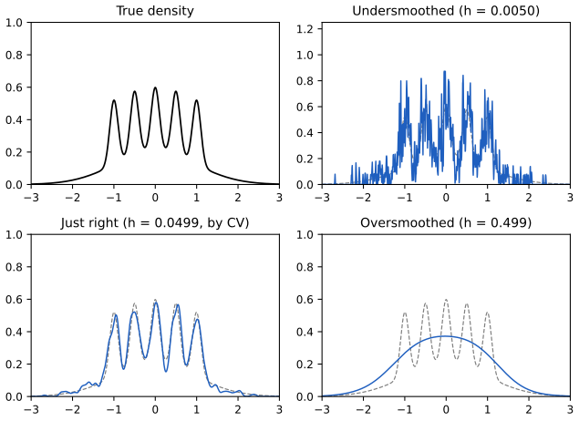
p. 125 The running example is a density with sharp features, the Bart Simpson density (Marron and Wand 1992 call it "the claw"):
\[ f(x)=\tfrac12\,\phi(x;0,1)+\tfrac1{10}\sum_{j=0}^4\phi\big(x;\tfrac j2-1,\tfrac1{10}\big), \tag{6.2} \]where \(\phi(x;\mu,\sigma)\) is the \(N(\mu,\sigma^2)\) density. Half the mass is a standard Normal hump, and the other half sits in five narrow claws at \(-1,-\tfrac12,0,\tfrac12,1\). From 1000 draws, cross-validation picks the bandwidth \(h=0.0499\) (the book reports 0.05); one tenth and ten times that bandwidth show what goes wrong on either side.
6.1 Cross-Validation
pp. 126–127 The loss of an estimator \(\fh\) with smoothing parameter \(h\) is the integrated squared error, and expanding the square separates what depends on \(h\):
\[ L(h)=\int(\fh(x)-f(x))^2\,\d x=\int\fh^2(x)\,\d x-2\int\fh(x)f(x)\,\d x+\int f^2(x)\,\d x . \]The last term is free of \(h\), so we minimise the expected value of
\[ J(h)=\int\fh^2(x)\,\d x-2\int\fh(x)f(x)\,\d x, \tag{6.3} \]and call \(\E J(h)=R(h)-\int f^2\) "the risk". The first term of \(J\) is computable; the second is not, because it involves \(f\).
Definition 6.4 (cross-validation score) p. 127
\[ \hJ(h)=\int\big(\fh(x)\big)^2\,\d x-\frac2n\sum_{i=1}^n\hat f_{(-i)}(X_i), \tag{6.5} \]where \(\hat f_{(-i)}\) is the estimator computed without \(X_i\).
Filling the gap 6.1: why the leave-one-out average estimates \(\int\fh f\), and when it is exactly unbiased p. 127; Exercise 3
Derivation
Let \(\hat f_{m}\) denote the estimator built from an iid sample of size \(m\) (with the same \(h\)). Fix \(i\). The estimator \(\hat f_{(-i)}\) is \(\hat f_{n-1}\) built from the other \(n-1\) points, which are independent of \(X_i\). Conditioning on them,
\[ \E\big[\hat f_{(-i)}(X_i)\given X_j,\ j\ne i\big]=\int\hat f_{(-i)}(x)f(x)\,\d x , \]so \(\E\hat f_{(-i)}(X_i)=\E\int\hat f_{n-1}f\), and the average over \(i\) has the same mean. Hence, for any estimator,
\[ \E\hJ(h)=\E\int\fh^2-2\,\E\int\hat f_{n-1}f,\qquad \E J(h)=\E\int\fh^2-2\,\E\int\hat f_{n}f . \]The two agree as soon as \(\E\hat f_m(x)\) does not depend on \(m\), since by Fubini \(\E\int\hat f_mf=\int\E\hat f_m(x)f(x)\,\d x\). This holds for the histogram (\(\E\fh(x)=p_j/h\) for \(x\in B_j\), Theorem 6.9) and for the kernel estimator (\(\E\fh(x)=\int K_h(x-t)f(t)\,\d t\)), whatever \(n\). So for both:
\[ \E\hJ(h)=\E J(h)=R(h)-\int f^2\qquad\text{exactly, for every }n\text{ and }h. \]For an estimator whose mean changes with \(n\) (a data-dependent bandwidth inside \(\fh\), for instance) the identity holds only approximately, with an error of the size of \(\E\hat f_{n-1}-\E\hat f_n\). Both identities were confirmed numerically: exactly for the histogram by computing both sides in closed form, and by simulation for the kernel estimator, where \(\E J\) is known in closed form for Normal mixtures (Filling the gap 6.7). ∎
6.2 Histograms
pp. 127–128 Take \(f\) supported on \([0,1]\), an integer \(m\), and bins
\[ B_1=\Big[0,\tfrac1m\Big),\ B_2=\Big[\tfrac1m,\tfrac2m\Big),\ \dots,\ B_m=\Big[\tfrac{m-1}m,1\Big]. \tag{6.6} \]With bin width \(h=1/m\), counts \(Y_j\), proportions \(\ph_j=Y_j/n\) and bin probabilities \(p_j=\int_{B_j}f\), the histogram is
\[ \fh(x)=\sum_{j=1}^m\frac{\ph_j}{h}\,I(x\in B_j). \tag{6.7} \]Since \(\E\ph_j=p_j=\int_{B_j}f\approx f(x)h\) for \(x\in B_j\) and small \(h\), \(\fh(x)\) is roughly unbiased. Everything below works on any interval \([a,b]\) with \(h=(b-a)/m\); the galaxy histograms use \([0,0.2]\).
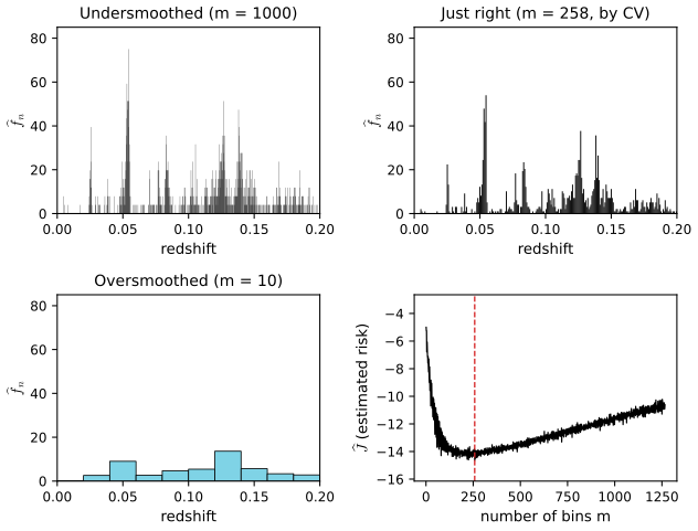
Example 6.8 (galaxy redshifts). The 1266 galaxies of Example 4.3 with redshift below 0.2. Too many bins give an undersmoothed histogram (low bias, high variance), too few an oversmoothed one; the cross-validated number is 258 here (the book reports 308; see the notes on the book).
Theorem 6.9 (mean and variance of the histogram) p. 129
For fixed \(x\) and \(m\), with \(B_j\) the bin containing \(x\),
\[ \E(\fh(x))=\frac{p_j}{h}\qquad\text{and}\qquad\V(\fh(x))=\frac{p_j(1-p_j)}{nh^2}. \tag{6.10} \]Filling the gap 6.2: proof of Theorem 6.9 p. 129
Proof
\(Y_j=\sum_iI(X_i\in B_j)\) is a sum of \(n\) independent Bernoulli\((p_j)\) variables, so \(Y_j\sim\text{Binomial}(n,p_j)\), \(\E Y_j=np_j\), \(\V Y_j=np_j(1-p_j)\). For \(x\in B_j\), \(\fh(x)=Y_j/(nh)\), hence \(\E\fh(x)=p_j/h\) and \(\V\fh(x)=np_j(1-p_j)/(nh)^2=p_j(1-p_j)/(nh^2)\). Nothing about \(f\) beyond integrability is used. ∎
Theorem 6.11 (risk of the histogram) p. 129
If \(f'\) is absolutely continuous and \(\int(f')^2\lt\infty\), then
\[ R(\fh,f)=\frac{h^2}{12}\int(f'(u))^2\,\d u+\frac1{nh}+o(h^2)+o\Big(\frac1n\Big). \tag{6.12} \]The minimiser of the leading terms is
\[ h^*=\frac1{n^{1/3}}\Big(\frac6{\int(f'(u))^2\,\d u}\Big)^{1/3}, \tag{6.13} \]and with this choice
\[ R(\fh,f)\sim\frac C{n^{2/3}},\qquad C=\Big(\frac34\Big)^{2/3}\Big(\int(f'(u))^2\,\d u\Big)^{1/3}. \tag{6.14} \](As printed, the remainder \(o(1/n)\) is not right: the integrated variance contains a term \(-\frac1n\int f^2\), which is of order exactly \(1/n\). It does not affect \(h^*\) or (6.14), since \(1/n=o(n^{-2/3})\). See Filling the gap 6.3.)
Filling the gap 6.3: the exact risk of a histogram, the remainder, \(h^*\) and \(C\) pp. 129, 140–142
Derivation
An exact formula. Split the risk into integrated squared bias and integrated variance. Since \(\fb=p_j/h\) on \(B_j\), \(\int_{B_j}\fb f=p_j^2/h\) and \(\int_{B_j}\fb^2=p_j^2/h\), so
\[ \int(\fb-f)^2=\int f^2-\frac1h\sum_jp_j^2,\qquad \int\V\fh=\sum_j h\,\frac{p_j(1-p_j)}{nh^2}=\frac1{nh}\Big(1-\sum_jp_j^2\Big). \]Hence, exactly,
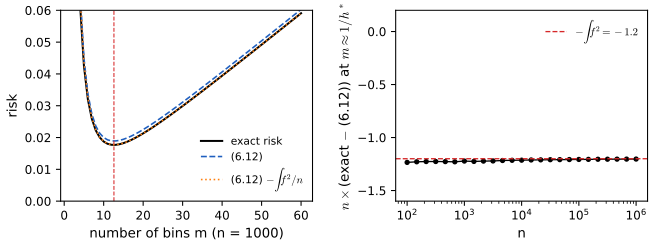
\[ R(\fh,f)=\int f^2-\frac1h\sum_jp_j^2+\frac1{nh}-\frac1{nh}\sum_jp_j^2 . \]The variance term. By the mean value theorem \(p_j=hf(\tilde x_j)\) for some \(\tilde x_j\in B_j\), so \(\frac1{nh}\sum_jp_j^2=\frac1n\sum_jhf(\tilde x_j)^2=\frac1n\big(\int f^2+o(1)\big)\), a Riemann sum. So the integrated variance is \(\frac1{nh}-\frac1n\int f^2+o(\frac1n)\): the second term is \(O(1/n)\), not \(o(1/n)\). Figure 6.S1 (right) shows \(n\times\)(exact risk minus (6.12)) settling at \(-\int f^2\).
The bias term. This is the appendix proof of the book. For \(x\in B_j\) with midpoint \(m_j\), a first-order Taylor expansion gives \(p_j/h-f(x)=f'(x)(m_j-x)+O(h^2)\) when \(f''\) is bounded, and \(\int_{B_j}(m_j-x)^2\d x=h^3/12\). Summing over the \(m=1/h\) bins with the mean value theorem, \(\int(\fb-f)^2=\frac{h^2}{12}\sum_jh f'(\tilde x_j)^2+O(h^3)=\frac{h^2}{12}\int f'^2+o(h^2)\). Under only \(\int f'^2\lt\infty\) and \(f'\) absolutely continuous, the same holds by approximating \(f'\) in \(L^2\) by smooth functions; the companion course gives the rigorous version in Filling the gap 20.3.
The optimum. Let \(A=\int f'^2\) and \(r(h)=h^2A/12+1/(nh)\). Then \(r'(h)=hA/6-1/(nh^2)=0\) gives \(h^3=6/(nA)\), which is (6.13), and \(r''\gt0\) makes it the minimum. At \(h^*\), \(h^{*2}A/12=\frac{6^{2/3}}{12}A^{1/3}n^{-2/3}\) and \(1/(nh^*)=6^{-1/3}A^{1/3}n^{-2/3}\), whose sum is
\[ \Big(\tfrac{6^{2/3}}{12}+6^{-1/3}\Big)A^{1/3}n^{-2/3}=\tfrac32\,6^{-1/3}A^{1/3}n^{-2/3}=\Big(\tfrac34\Big)^{2/3}A^{1/3}n^{-2/3}, \]since \((\tfrac32)^3/6=\tfrac{27}{48}=\tfrac9{16}=(\tfrac34)^2\). This is (6.14). ∎
With the optimal width the risk falls like \(n^{-2/3}\), slower than the \(n^{-4/5}\) of kernel estimators (Section 6.3). The width (6.13) depends on the unknown \(\int f'^2\), so in practice \(h\) is chosen by cross-validation, which for histograms has a closed form.
See also (companion course): Probability and Statistical Inference, Theorem 20.4 and the rates demo.
Theorem 6.15 (the score in closed form) p. 129
\[ \hJ(h)=\frac2{h(n-1)}-\frac{n+1}{h(n-1)}\sum_{j=1}^m\ph_j^{\,2}. \tag{6.16} \]Filling the gap 6.4: deriving (6.16) step by step from the definition (6.5) p. 129
Derivation
Write \(Y_j=n\ph_j\) for the count of bin \(j\), and \(j(i)\) for the bin that contains \(X_i\). Every observation lies in exactly one bin, so \(\sum_jY_j=n\). We compute the two terms of (6.5) bin by bin.
Step 1: the integral of the squared estimate. On \(B_j\) the histogram is the constant \(\ph_j/h\), and \(B_j\) has length \(h\). The bins partition \([0,1]\) and \(\fh=0\) outside, so
\[ \int\fh^2(x)\,\d x=\sum_{j=1}^m\int_{B_j}\Big(\frac{\ph_j}h\Big)^2\d x=\sum_{j=1}^m\frac{\ph_j^{\,2}}{h^2}\,h=\frac1h\sum_{j=1}^m\ph_j^{\,2}=\frac1{n^2h}\sum_{j=1}^mY_j^2 . \]Step 2: one leave-one-out value. Remove \(X_i\). The remaining \(n-1\) points form a histogram with the same bins, in which bin \(j(i)\) holds \(Y_{j(i)}-1\) points and every other bin is unchanged. Evaluated at \(X_i\), which lies in \(B_{j(i)}\), it is
\[ \hat f_{(-i)}(X_i)=\frac{Y_{j(i)}-1}{(n-1)h}. \]Step 3: the leave-one-out sum, grouped by bins. The value in Step 2 depends on \(i\) only through its bin. Bin \(j\) contains \(Y_j\) observations, each contributing \((Y_j-1)/((n-1)h)\), so
\[ \sum_{i=1}^n\hat f_{(-i)}(X_i)=\sum_{j=1}^m Y_j\,\frac{Y_j-1}{(n-1)h}=\frac1{(n-1)h}\Big(\sum_jY_j^2-\sum_jY_j\Big)=\frac1{(n-1)h}\Big(\sum_jY_j^2-n\Big). \](Empty bins contribute nothing, consistently with \(Y_j(Y_j-1)=0\).)
Step 4: assemble. Insert Steps 1 and 3 into (6.5):
\[ \hJ(h)=\frac1{n^2h}\sum_jY_j^2-\frac2n\cdot\frac{\sum_jY_j^2-n}{(n-1)h}=\frac2{(n-1)h}-\sum_jY_j^2\Big[\frac2{n(n-1)h}-\frac1{n^2h}\Big]. \]The bracket is \(\dfrac{2n-(n-1)}{n^2(n-1)h}=\dfrac{n+1}{n^2(n-1)h}\). Finally \(\sum_jY_j^2/n^2=\sum_j\ph_j^{\,2}\), so
\[ \hJ(h)=\frac2{(n-1)h}-\frac{n+1}{(n-1)h}\sum_j\ph_j^{\,2}, \]which is (6.16). On an interval \([a,b]\) the same steps hold with \(h=(b-a)/m\).
Unbiasedness, directly (Exercise 3). With \(\E\ph_j^{\,2}=p_j(1-p_j)/n+p_j^2\),
\[ \E\hJ=\frac2{(n-1)h}-\frac{n+1}{(n-1)h}\sum_j\Big(\frac{p_j}n+\frac{n-1}np_j^2\Big)=\frac2{(n-1)h}-\frac{n+1}{n(n-1)h}-\frac{n+1}{nh}\sum_jp_j^2=\frac1{nh}-\frac{n+1}{nh}\sum_jp_j^2 , \]using \(\sum_jp_j=1\) and \(\frac{2n-(n+1)}{n(n-1)}=\frac1n\). On the other side, \(\E J=\E\int\fh^2-2\int\fb f=\frac1h\sum_j\E\ph_j^{\,2}-\frac2h\sum_jp_j^2=\frac1{nh}-\frac{n+1}{nh}\sum_jp_j^2\). The two agree, as Filling the gap 6.1 predicts. The closed form and the brute-force definition (refitting \(n\) times) agree to rounding on the galaxy data. ∎
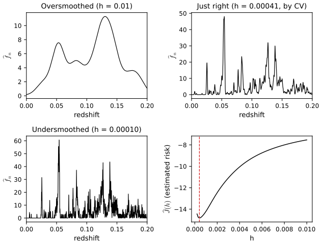
Example 6.17. On the galaxy data the score is minimised at \(m=258\) (Figure 6.2, bottom right). The curve is very flat near the minimum: every \(m\) from about 80 to 335 is within 3% of it (Figure 4.1).
See also (companion course): Probability and Statistical Inference, Filling the gap 20.4 (the same score) and the histogram cross-validation demo.
p. 130 A confidence band. For the reasons of Section 5.7 (the bias cannot be estimated as well as the estimate), we aim at the histogram-resolution version of \(f\),
\[ \fb(x)=\E(\fh(x))=\sum_{j=1}^m\frac{p_j}hI(x\in B_j), \tag{6.18} \]and call \((\ell,u)\) a \(1-\alpha\) band for \(\fb\) if
\[ \P\big(\ell(x)\le\fb(x)\le u(x)\ \text{for all }x\big)\ge1-\alpha. \tag{6.19} \]Theorem 6.20 (a band for the histogram) p. 130
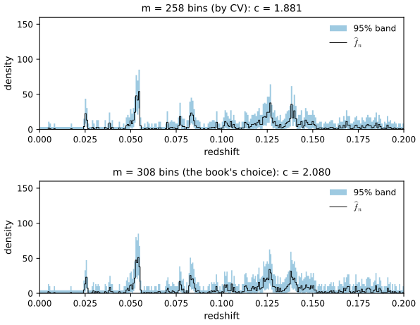
Let \(m=m(n)\to\infty\) with \(m(n)\log n/n\to0\). Define
\[ \ell_n(x)=\Big(\max\big\{\sqrt{\fh(x)}-c,\,0\big\}\Big)^2,\qquad u_n(x)=\Big(\sqrt{\fh(x)}+c\Big)^2, \tag{6.21} \] \[ c=\frac{z_{\alpha/(2m)}}2\sqrt{\frac mn}. \tag{6.22} \]Then \((\ell_n,u_n)\) is an approximate \(1-\alpha\) band for \(\fb\). (On \([a,b]\) with \(h=(b-a)/m\): \(c=z_{\alpha/(2m)}/(2\sqrt{nh})\).)
Filling the gap 6.5: the full proof of Theorem 6.20: variance stabilisation, the delta method and Bonferroni pp. 130–131
Proof
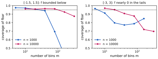
The book gives an outline. Here is the complete argument, in five steps, with the extra assumption it needs: \(f\ge f_{\min}\gt0\) on \([0,1]\), so that every \(p_j\ge f_{\min}/m\). (Figure 6.S2 shows what happens without it.)
Step 1: reduce the event to the bins. Both \(\fh\) and \(\fb\) are constant on each bin, with values \(\hat f_{n,j}=\ph_j/h\) and \(\bar f_{n,j}=p_j/h\). Fix \(j\) and write \(s=\sqrt{\hat f_{n,j}}\ge0\), \(t=\sqrt{\bar f_{n,j}}\ge0\). Since squaring is increasing on \([0,\infty)\),
\[ (\max\{s-c,0\})^2\le t^2\le(s+c)^2\iff\max\{s-c,0\}\le t\le s+c\iff |t-s|\le c, \]where the last step uses \(t\ge0\) (the constraint \(t\ge0\) is automatic, so \(\max\{s-c,0\}\le t\) is the same as \(s-c\le t\)). Therefore the event of (6.19) is
\[ A=\Big\{\max_{1\le j\le m}\big|\sqrt{\hat f_{n,j}}-\sqrt{\bar f_{n,j}}\big|\le c\Big\}. \](The book writes \(\sqrt{f}\) instead of \(\sqrt{\fb}\) in this display; the band is for \(\fb\).) Since \(\sqrt{\hat f_{n,j}}-\sqrt{\bar f_{n,j}}=(\sqrt{\ph_j}-\sqrt{p_j})/\sqrt h=\sqrt m(\sqrt{\ph_j}-\sqrt{p_j})\), and \(2\sqrt n\,c/\sqrt m=z_{\alpha/(2m)}\) by (6.22),
\[ A^c=\Big\{\max_jT_j\gt z_{\alpha/(2m)}\Big\},\qquad T_j=2\sqrt n\,\big|\sqrt{\ph_j}-\sqrt{p_j}\big| . \]Step 2: Bonferroni. By the union bound,
\[ \P(A^c)\le\sum_{j=1}^m\P\big(T_j\gt z_{\alpha/(2m)}\big). \]No independence between bins is needed. (The counts are multinomial and in fact negatively dependent; the book's remark that the \(\sqrt{\ph_j}\) are "approximately independent" is not used.)
Step 3: the square root stabilises the variance (delta method). \(n\ph_j\sim\text{Binomial}(n,p_j)\), so by the central limit theorem \(\sqrt n(\ph_j-p_j)\leadsto N(0,p_j(1-p_j))\). With \(g(t)=\sqrt t\), \(g'(p)=1/(2\sqrt p)\), the delta method gives
\[ \sqrt n\big(\sqrt{\ph_j}-\sqrt{p_j}\big)\leadsto N\Big(0,\ g'(p_j)^2p_j(1-p_j)\Big)=N\Big(0,\ \frac{1-p_j}4\Big), \]so \(2\sqrt n(\sqrt{\ph_j}-\sqrt{p_j})\approx N(0,1-p_j)\). The variance no longer depends on the unknown height of the bin, except through \(1-p_j\le1\). Hence
\[ \P(T_j\gt z)\approx2\Big\{1-\Phi\Big(\frac z{\sqrt{1-p_j}}\Big)\Big\}\le2\{1-\Phi(z)\}. \]The book's "assume \(1-p_j\approx1\)" is therefore on the safe side: it only makes the band conservative.
Step 4: add up. With \(z=z_{\alpha/(2m)}\), \(2\{1-\Phi(z)\}=\alpha/m\), and
\[ \P(A^c)\lesssim\sum_{j=1}^m\frac\alpha m=\alpha . \]Step 5: why the conditions on \(m\), and what makes "\(\approx\)" rigorous. Step 3 is used at the level \(\alpha/m\to0\), far in the tail, and simultaneously for \(m\to\infty\) bins, each with a small \(p_j\). Two things must hold uniformly in \(j\). Write the exact identity
\[ 2\sqrt n\big(\sqrt{\ph_j}-\sqrt{p_j}\big)=\underbrace{\frac{\sqrt n(\ph_j-p_j)}{\sqrt{p_j(1-p_j)}}}_{S_j}\cdot\sqrt{1-p_j}\cdot\underbrace{\frac{2}{1+\sqrt{\ph_j/p_j}}}_{Q_j}, \]which follows from \(\sqrt{\ph}-\sqrt p=(\ph-p)/(\sqrt{\ph}+\sqrt p)\).
- The ratio \(Q_j\to1\) uniformly. Bernstein's inequality gives \(\P(|\ph_j-p_j|\gt\varepsilon p_j)\le2\exp\{-n\varepsilon^2p_j/(2+2\varepsilon/3)\}\). With \(p_j\ge f_{\min}/m\) and a union bound, \(\P(\max_j|\ph_j/p_j-1|\gt\varepsilon)\le2m\exp\{-c_\varepsilon n/m\}\to0\) as soon as \(n/(m\log m)\to\infty\). Since \(\log m\le\log n\), this is exactly the book's condition \(m\log n/n\to0\): it guarantees that every bin holds many points, so that the linearisation of the square root is accurate in all bins at once.
- The tail of \(S_j\) is Normal at the level \(\alpha/m\). The central limit theorem alone controls \(\P(S_j\gt z)\) only up to an absolute error, which must be small compared with \(\alpha/m\). Cramér's moderate-deviation theorem for sums of iid bounded variables (Petrov 1975, Chapter VIII) gives \(\P(S_j\gt z)/(1-\Phi(z))\to1\) uniformly in \(0\le z\le o((np_j)^{1/6})\). Here \(z=z_{\alpha/(2m)}\approx\sqrt{2\log m}\) and \(np_j\gtrsim n/m\), so it suffices that \(m(\log m)^3/n\to0\), a slightly stronger condition than the book's. The perturbation by \(Q_j=1+O_P(\sqrt{m\log m/n})\) moves the threshold by a factor that changes the Normal tail probability by \(\exp\{O(z^2\sqrt{m\log m/n})\}\to1\) under the same condition.
Under these conditions \(\P(A^c)\le\sum_j\frac\alpha m(1+o(1))=\alpha+o(1)\): the band has asymptotic coverage at least \(1-\alpha\). ∎
When it fails. If \(f\) is near 0 in some bins, those bins hold a handful of points and the Normal approximation is poor there. An empty bin has band \([0,c^2]\), which misses \(\bar f_{n,j}\) whenever \(np_j\gt z^2/4\); a bin with one or two points can miss in the other direction. Figure 6.S2 shows both regimes.
See also (companion course): Probability and Statistical Inference, Filling the gap 20.5.
6.3 Kernel Density Estimation
Definition 6.25 (kernel density estimator) p. 132
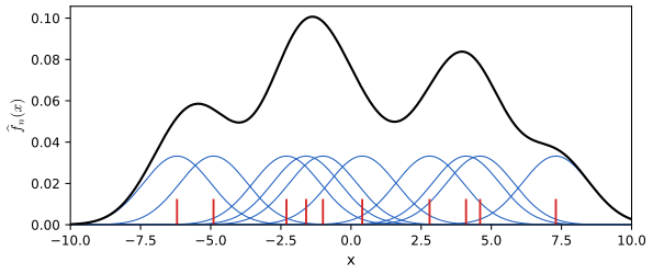
Given a kernel \(K\) (conditions (4.22), Definition 4.22) and a bandwidth \(h\gt0\),
\[ \fh(x)=\frac1n\sum_{i=1}^n\frac1hK\Big(\frac{x-X_i}h\Big). \tag{6.26} \]Each observation carries a bump of mass \(1/n\), and the estimate is their sum (Figure 6.4). It is a density whenever \(K\) is, and it inherits the smoothness of \(K\). The shape of \(K\) matters little (the efficiency of the common kernels relative to the optimal Epanechnikov kernel is above 93 percent; see Filling the gap 20.6 of the companion course); the bandwidth matters a great deal (Figures 6.1 and 6.5).
Theorem 6.27 (consistency) p. 133
If \(f\) is continuous at \(x\), \(h_n\to0\) and \(nh_n\to\infty\), then \(\fh(x)\overset{P}\to f(x)\).
Filling the gap 6.6: proof of Theorem 6.27 (Exercise 1) p. 133
Proof
Assume \(K\) is bounded, \(\|K\|_\infty\lt\infty\), with \(\int|u|K(u)\,\d u\lt\infty\) or compact support, and \(f\) bounded. (Without boundedness of \(f\), the argument works with a slightly more careful truncation; the companion course gives the general version in Filling the gap 20.8.) By Chebyshev's inequality it is enough that the bias and the variance tend to 0.
Bias. Substituting \(t=x-hu\), \(\E\fh(x)=\int K(u)f(x-hu)\,\d u\), so \(\E\fh(x)-f(x)=\int K(u)\{f(x-hu)-f(x)\}\,\d u\). Given \(\varepsilon\gt0\), pick \(\delta\) with \(|f(y)-f(x)|\lt\varepsilon\) for \(|y-x|\lt\delta\). Split the integral at \(|u|\lt\delta/h\): the inner part is at most \(\varepsilon\); the outer part is at most \(2\|f\|_\infty\int_{|u|\ge\delta/h}K\to0\) as \(h\to0\). So the bias tends to 0.
Variance. \(\fh(x)\) is an average of the iid variables \(K_h(x-X_i)\), so
\[ \V\fh(x)\le\frac1n\E K_h(x-X)^2=\frac1{nh}\int K^2(u)f(x-hu)\,\d u\le\frac{\|K\|_\infty\,\|f\|_\infty}{nh}\to0 . \]Hence \(\E(\fh(x)-f(x))^2\to0\), which implies convergence in probability. ∎
Theorem 6.28 (pointwise and integrated risk) p. 133
Let \(R_x=\E(f(x)-\fh(x))^2\) and \(R=\int R_x\,\d x\). If \(f''\) is absolutely continuous, \(\int(f''')^2\lt\infty\), and \(K\) satisfies (4.22), then
\[ R_x=\tfrac14\sigma_K^4h_n^4(f''(x))^2+\frac{f(x)\int K^2}{nh_n}+O\Big(\frac1n\Big)+O(h_n^6), \] \[ R=\tfrac14\sigma_K^4h_n^4\int(f''(x))^2\d x+\frac{\int K^2}{nh}+O\Big(\frac1n\Big)+O(h_n^6). \tag{6.29} \]Filling the gap 6.7: the bias and variance expansions with remainders, and the exact risk for Normal mixtures pp. 133–134
Derivation
Bias. With \(K\) symmetric, \(\int K=1\), \(\int uK=0\), \(\sigma_K^2=\int u^2K\) and \(\int u^4K\lt\infty\), and \(f\) four times differentiable with \(f^{(4)}\) bounded, Taylor's theorem with Lagrange remainder gives
\[ f(x-hu)=f(x)-huf'(x)+\tfrac{h^2u^2}2f''(x)-\tfrac{h^3u^3}6f'''(x)+\tfrac{h^4u^4}{24}f^{(4)}(\xi_u). \]Integrating against \(K\), the odd terms vanish by symmetry:
\[ b(x)=\E\fh(x)-f(x)=\tfrac12\sigma_K^2h^2f''(x)+O(h^4),\qquad b(x)^2=\tfrac14\sigma_K^4h^4f''(x)^2+O(h^6). \](The book's assumption \(\int f'''^2\lt\infty\) gives the integrated version: write the remainder after the \(f''\) term in integral form and bound its \(L^2\) norm by Minkowski's integral inequality, which gives \(\|b-\tfrac12\sigma_K^2h^2f''\|_2=O(h^3)\) and hence an \(O(h^5)\) cross term; the \(O(h^6)\) of (6.29) needs one more derivative or a symmetric kernel argument, a detail that does not affect the leading terms.)
Variance, exactly. \(\V\fh(x)=\frac1n\{\E K_h(x-X)^2-(\E K_h(x-X))^2\}\) and \(\E K_h(x-X)^2=\frac1h\int K^2(u)f(x-hu)\,\d u=\frac{f(x)R(K)}h+O(1)\) for bounded \(f'\) (the \(O(1)\) uses \(\int|u|K^2\lt\infty\)). So \(\V\fh(x)=\frac{f(x)R(K)}{nh}+O(\frac1n)\). Integrating over \(x\), and using \(\int f(x-hu)\,\d x=1\),
\[ \int\V\fh=\frac{R(K)}{nh}-\frac1n\int\fb^2\qquad\text{exactly.} \]Adding the integrated squared bias gives (6.29). The companion course has the details of the dominated-convergence step in Filling the gap 20.7.
An exact formula for Normal mixtures. If \(f=\sum_lw_l\phi(\cdot;\mu_l,s_l)\) and \(K=\phi\), every integral is a Normal convolution (Marron and Wand 1992): with \(\Omega_a\) the matrix of entries \(\phi(\mu_l-\mu_{l'};0,(ah^2+s_l^2+s_{l'}^2)^{1/2})\),
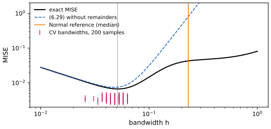
\[ R(h)=\frac1{2\sqrt\pi\,nh}+w^\T\Big[\big(1-\tfrac1n\big)\Omega_2-2\Omega_1+\Omega_0\Big]w . \]Figure 6.S3 uses it for the Bart Simpson density, a 6-component mixture: the exact risk is minimised at \(h=0.0516\) (risk 0.0067), the asymptotic formula (6.29) at \(h^*=0.0476\) (0.0074). The two curves agree for small \(h\) and part for large \(h\), where \(h^4\) no longer describes the bias of a density with claws of width 0.1. ∎
Differentiating the leading terms of (6.29) gives the asymptotically optimal bandwidth
\[ h^*=\Big(\frac{c_2}{c_1^2A(f)n}\Big)^{1/5},\qquad c_1=\int x^2K,\ c_2=\int K^2,\ A(f)=\int(f'')^2 , \tag{6.30} \]which falls like \(n^{-1/5}\), and a risk of order \(n^{-4/5}\), faster than the histogram's \(n^{-2/3}\).
Filling the gap 6.8: the optimal bandwidth and the optimal risk p. 134, (6.30)
Derivation
Let \(r(h)=\frac14c_1^2Ah^4+\frac{c_2}{nh}\). Then \(r'(h)=c_1^2Ah^3-\frac{c_2}{nh^2}=0\) gives \(h^5=c_2/(c_1^2An)\), which is (6.30), and \(r''\gt0\). At \(h^*\) the identity \(c_2/n=c_1^2Ah^{*5}\) turns the variance term into \(c_2/(nh^*)=c_1^2Ah^{*4}\), four times the bias term, so
\[ r(h^*)=\tfrac54c_1^2A\,h^{*4}=\tfrac54\big(c_1^2A\big)^{1/5}\Big(\frac{c_2}n\Big)^{4/5}=\tfrac54\big(c_1c_2^2\big)^{2/5}A^{1/5}n^{-4/5}. \]At the optimum the squared bias is one fifth of the risk and the variance four fifths. The kernel enters only through \((c_1c_2^2)^{2/5}=(\sigma_KR(K))^{4/5}\), which is scale-free and is minimised by the Epanechnikov kernel. ∎
Theorem 6.31 (no estimator beats \(n^{-2m/(2m+1)}\)) pp. 134–135
Let \(\mathcal F_m(c)=\{f\text{ a density}:\int|f^{(m)}(x)|^2\d x\le c^2\}\). For any estimator \(\fh\),
\[ \sup_{f\in\mathcal F_m(c)}\E_f\int(\fh(x)-f(x))^2\d x\ge b\Big(\frac1n\Big)^{2m/(2m+1)} \tag{6.32} \]for a constant \(b\gt0\) depending only on \(m\) and \(c\). With \(m=2\): \(n^{-4/5}\) is the best possible rate.
Filling the gap 6.10: a proof of the lower bound by Assouad's lemma p. 134
Proof
The book refers to van der Vaart (1998, Chapter 24). Here is a self-contained version of the standard argument; the companion course gives the \(m=2\) case in Filling the gap 20.9.
A hypercube of densities. Let \(f_0\) be a smooth density with \(f_0\ge\kappa\gt0\) on \([0,1]\) and \(\int|f_0^{(m)}|^2\le c^2/4\) (for \(c\) not too small; otherwise rescale). Let \(\psi\) be infinitely differentiable, supported in \([0,1]\), with \(\int\psi=0\) and \(\psi\ne0\). For an integer \(M\), \(\delta=1/M\) and \(L\gt0\) put
\[ \psi_j(x)=L\,\delta^m\psi\big((x-(j-1)\delta)/\delta\big),\qquad f_\omega=f_0+\sum_{j=1}^M\omega_j\psi_j,\quad\omega\in\{0,1\}^M . \]The bumps have disjoint supports and integrate to 0, so \(\int f_\omega=1\); and \(|\psi_j|\le L\delta^m\|\psi\|_\infty\le\kappa/2\) for small \(L\), so \(f_\omega\ge\kappa/2\) on \([0,1]\). Since \(\psi_j^{(m)}(x)=L\psi^{(m)}(\cdot)\) (the \(\delta^m\) cancels the chain rule) and the supports are disjoint, \(\int|\sum_j\omega_j\psi_j^{(m)}|^2\le ML^2\delta\int|\psi^{(m)}|^2=L^2\int|\psi^{(m)}|^2\). With \((a+b)^2\le2a^2+2b^2\) and \(L\) small, every \(f_\omega\in\mathcal F_m(c)\).
The loss splits over the cells. Let \(I_j=[(j-1)\delta,j\delta)\) and \(\|\psi_j\|^2=L^2\delta^{2m+1}\|\psi\|_2^2=:\beta\). Given any \(\fh\), let \(\hat\omega_j\in\{0,1\}\) make \(f_0+\hat\omega_j\psi_j\) closest to \(\fh\) in \(L^2(I_j)\). By the triangle inequality, if \(\hat\omega_j\ne\omega_j\) then \(\sqrt\beta=\|\psi_j\|\le\|\fh-f_\omega\|_{I_j}+\|\fh-f_{\hat\omega}\|_{I_j}\le2\|\fh-f_\omega\|_{I_j}\). Hence
\[ \int(\fh-f_\omega)^2\ge\sum_j\int_{I_j}(\fh-f_\omega)^2\ge\frac\beta4\sum_jI(\hat\omega_j\ne\omega_j). \]Assouad's lemma. For any estimator \(\hat\omega\) of \(\omega\in\{0,1\}^M\),
\[ \max_\omega\E_\omega\sum_jI(\hat\omega_j\ne\omega_j)\ge\frac M2\min_{\omega\sim\omega'}\big(1-\TV(P_\omega^n,P_{\omega'}^n)\big), \]where \(\omega\sim\omega'\) differ in one coordinate. (Proof: average over \(\omega\) uniform; for each \(j\), pair \(\omega\) with its neighbour that flips \(j\); the sum of the two error probabilities of any test is at least \(1-\TV\).)
Neighbours are hard to tell apart. For neighbours, \(\KL(P_\omega,P_{\omega'})\le\chi^2(P_\omega,P_{\omega'})=\int\psi_j^2/f_{\omega'}\le2\beta/\kappa\), so \(\KL(P^n_\omega,P^n_{\omega'})\le2n\beta/\kappa\) and, by Pinsker's inequality, \(\TV\le\sqrt{n\beta/\kappa}\). Choose \(M\) so that \(\delta=n^{-1/(2m+1)}\) (up to rounding): then \(n\beta=L^2\|\psi\|^2\,n\delta^{2m+1}=L^2\|\psi\|^2\), a constant, and with \(L\) small \(\TV\le\frac12\).
Conclusion. Combining, \(\sup_\omega\E_\omega\int(\fh-f_\omega)^2\ge\frac\beta4\cdot\frac M2\cdot\frac12=\frac{M\beta}{16}=\frac{L^2\|\psi\|^2}{16}\delta^{2m}=b\,n^{-2m/(2m+1)}\). ∎
The rate is attained: a kernel of order \(m\) (moments 1 to \(m-1\) zero) with \(h\asymp n^{-1/(2m+1)}\) has risk of the same order, so \(n^{-2m/(2m+1)}\) is the minimax rate over \(\mathcal F_m(c)\).
p. 135 The Normal reference rule. If \(f\) were \(N(\mu,\sigma^2)\) and \(K=\phi\), (6.30) would give
\[ h_n=1.06\,\hat\sigma\,n^{-1/5},\qquad\hat\sigma=\min\{s,\ Q/1.34\}, \]with \(s\) the sample standard deviation and \(Q\) the interquartile range.
Filling the gap 6.9: where 1.06 and 1.34 come from p. 135
Derivation
For \(f=\phi_\sigma\) (the \(N(0,\sigma^2)\) density), \(f''(x)=\sigma^{-3}\phi(z)(z^2-1)\) with \(z=x/\sigma\), so \(A(f)=\sigma^{-5}\int\phi(z)^2(z^2-1)^2\d z\). Now \(\phi(z)^2=\frac1{2\sqrt\pi}\phi(z;0,2^{-1/2})\), and under \(N(0,\frac12)\), \(\E z^2=\frac12\), \(\E z^4=\frac34\), so \(\E(z^2-1)^2=\frac34-1+1=\frac34\) and
\[ A(\phi_\sigma)=\frac3{8\sqrt\pi\,\sigma^5}. \]For the Gaussian kernel \(c_1=1\), \(c_2=\frac1{2\sqrt\pi}\). Then (6.30) gives \(h^5=\frac{1/(2\sqrt\pi)}{3n/(8\sqrt\pi\sigma^5)}=\frac{4\sigma^5}{3n}\), so \(h=(4/3)^{1/5}\sigma n^{-1/5}=1.0592\,\sigma n^{-1/5}\). For the Normal, \(Q=2z_{0.25}\sigma=1.349\sigma\), so \(Q/1.34\) is consistent for \(\sigma\); taking the smaller of \(s\) and \(Q/1.34\) guards against heavy tails and outliers, which inflate \(s\). ∎
The rule oversmooths anything rougher than a Normal. On the Bart Simpson sample it gives \(h=0.226\), four and a half times the cross-validated 0.0499, and erases the claws (Figure 6.S3; demo preset 4).
pp. 135–136 For kernel estimators the cross-validation score is
\[ \hJ(h)=\int\fh^2(x)\,\d x-\frac2n\sum_{i=1}^n\hat f_{-i}(X_i). \tag{6.33} \]Theorem 6.34 (the score is unbiased, and a formula for it) pp. 135–136
For any \(h\gt0\), \(\E[\hJ(h)]=\E[J(h)]\). Also
\[ \hJ(h)=\frac1{hn^2}\sum_i\sum_jK^*\Big(\frac{X_i-X_j}h\Big)+\frac2{nh}K(0)+O\Big(\frac1{n^2}\Big), \tag{6.35} \]where \(K^*(x)=K^{(2)}(x)-2K(x)\) and \(K^{(2)}(z)=\int K(z-y)K(y)\,\d y\). (The remainder is in fact of order \(1/n\), not \(1/n^2\); see below.)
Filling the gap 6.11: the exact score, (6.35) and its remainder (Exercise 4) p. 136
Derivation
Unbiasedness is Filling the gap 6.1: \(\E\fh(x)=\int K_h(x-t)f(t)\,\d t\) does not depend on \(n\).
The first term. Expanding the square and substituting \(x=X_j+hy\),
\[ \int\fh^2=\frac1{n^2h^2}\sum_{i,j}\int K\Big(\frac{x-X_i}h\Big)K\Big(\frac{x-X_j}h\Big)\d x=\frac1{n^2h}\sum_{i,j}\int K\Big(\frac{X_j-X_i}h+y\Big)K(y)\,\d y=\frac1{n^2h}\sum_{i,j}K^{(2)}\Big(\frac{X_i-X_j}h\Big), \]using the symmetry of \(K\). For \(K=\phi\), \(K^{(2)}\) is the \(N(0,2)\) density (Remark 6.36), the density of the sum of two independent standard Normals. For the Epanechnikov kernel \(K^{(2)}(z)=\frac3{160}(2-|z|)^3(z^2+6|z|+4)\) and for the boxcar \(\frac12I(|u|\le1)\), \(K^{(2)}(z)=\frac14(2-|z|)\), both on \(|z|\le2\).
The second term. \(\hat f_{-i}(X_i)=\frac1{(n-1)h}\sum_{j\ne i}K\big(\frac{X_i-X_j}h\big)\). So the exact score is
\[ \hJ(h)=\frac1{n^2h}\sum_{i,j}K^{(2)}\Big(\frac{X_i-X_j}h\Big)-\frac2{n(n-1)h}\sum_{i\ne j}K\Big(\frac{X_i-X_j}h\Big). \]This is what the code and the demonstrations compute; it needs only the pairwise differences.
Deriving (6.35). Write \(\frac1{n(n-1)}=\frac1{n^2}+\frac1{n^2(n-1)}\) and \(\sum_{i\ne j}=\sum_{i,j}-\sum_{i=j}\), where the diagonal contributes \(nK(0)\):
\[ -\frac2{n(n-1)h}\sum_{i\ne j}K=-\frac2{n^2h}\sum_{i,j}K+\frac{2K(0)}{nh}-\underbrace{\frac2{n^2(n-1)h}\sum_{i\ne j}K\Big(\frac{X_i-X_j}h\Big)}_{\Delta}. \]Adding the first term gives exactly \(\frac1{hn^2}\sum_{i,j}K^*+\frac{2K(0)}{nh}-\Delta\), so (6.35) holds with remainder \(-\Delta\).
The size of the remainder. \(\E\big[h^{-1}K((X_1-X_2)/h)\big]=\int\fb f\to\int f^2\), so
\[ \E\Delta=\frac{2\,n(n-1)}{n^2(n-1)}\int\fb f=\frac2n\int\fb f\approx\frac2n\int f^2, \]which is of order \(1/n\), not \(1/n^2\). On the galaxy data at the cross-validated bandwidth, \(n\Delta=29.9\), against \(2\int\fh^2\approx22\) for a smoother estimate. The remainder is harmless for choosing \(h\) only because it varies slowly with \(h\) (\(\int\fb f=\int f^2-O(h^2)\)); the exact formula above costs no more and should be preferred. ∎
Remark 6.36. For the Normal kernel \(K^{(2)}\) is the \(N(0,2)\) density; \(\fh\) and the score can be computed quickly with the fast Fourier transform after binning (Silverman 1986, pp. 61–66).
Theorem 6.37 (Stone's theorem; Stone 1984) p. 136
If \(f\) is bounded, \(\hat f_h\) is the kernel estimator with bandwidth \(h\) and \(\hat h\) is chosen by cross-validation, then
\[ \frac{\int\big(f(x)-\hat f_{\hat h}(x)\big)^2\d x}{\inf_h\int\big(f(x)-\hat f_h(x)\big)^2\d x}\overset{\text{a.s.}}\longrightarrow1. \tag{6.38} \]Filling the gap 6.12: why Stone's theorem holds, in outline, and what it does not say p. 136
Outline
By the algebra of Filling the gap 6.1, \(\hJ(h)+\int f^2=L(h)+D(h)\), where \(L(h)=\int(\hat f_h-f)^2\) is the loss and
\[ D(h)=2\Big\{\int\hat f_hf-\frac1n\sum_i\hat f_{h,(-i)}(X_i)\Big\} \]has mean zero. Stone's argument shows that \(\sup_h|D(h)-D(h')|/L(h)\to0\) almost surely over the relevant range of \(h\), for a fixed reference \(h'\): the centred U-statistic \(D\) fluctuates on a smaller scale than the loss. Then \(\hat h\), which minimises \(L+D\), nearly minimises \(L\), and the ratio (6.38) tends to 1. The exponential inequalities for U-statistics and a grid argument over \(h\) do the work; the companion course sketches them in Filling the gap 20.11.
What the theorem does not say: the convergence is slow. Hall and Marron (1987) showed \((\hat h-h_0)/h_0=O_P(n^{-1/10})\), so in finite samples \(\hat h\) varies a lot. In Figure 6.S3 the 200 cross-validated bandwidths range from 0.026 to 0.065 around an optimum of 0.052. And rounded data (ties) can drive the score to \(-\infty\) as \(h\to0\), because \(\hat f_{(-i)}(X_i)\) picks up \(K(0)/h\) from each tie.
A wiggly cross-validated estimate is not evidence that cross-validation failed: the eye is a poor judge of integrated squared error. Plug-in bandwidths estimate \(A(f)=\int f''^2\) in (6.30); since \(f''\) is harder to estimate than \(f\), they rest on stronger assumptions (Loader 1999b; Hjort 1999). Adaptive kernels let \(h\) vary with \(x\) or with \(X_i\) (Chapter 9).
p. 137 Bands for kernel estimators. The book refers to Section 6.6. A direct construction is also possible, and it uses the same two tools as the histogram band: a square root that stabilises the variance, and a simultaneous constant, here from the tube formula of Chapter 5 rather than Bonferroni.
Filling the gap 6.13: an approximate band for \(\E\fh\) from the square root and the tube formula p. 137
Derivation
Variance stabilisation. By Filling the gap 6.7, \(\V\fh(x)\approx\fb(x)R(K)/(nh)\). The delta method with \(g(t)=\sqrt t\) gives
\[ \V\sqrt{\fh(x)}\approx\frac{\V\fh(x)}{4\fb(x)}\approx\frac{R(K)}{4nh}=:s^2, \]the same for every \(x\). So \(Z(x)=(\sqrt{\fh(x)}-\sqrt{\fb(x)})/s\) is approximately a Gaussian process with unit variance.
Its correlation. \(\Cov(\fh(x),\fh(y))=\frac1n\Cov(K_h(x-X),K_h(y-X))\approx\frac{f(x)}{nh}K^{(2)}\big(\frac{x-y}h\big)\) for \(|x-y|=O(h)\), so locally \(Z\) is stationary with correlation \(\rho(t)=K^{(2)}(t/h)/K^{(2)}(0)\).
The tube formula. For a smooth unit-variance Gaussian process on an interval of length \(\ell\), \(\P(\sup|Z|\gt c)\approx2\{1-\Phi(c)\}+\frac{\kappa_0}\pi e^{-c^2/2}\) (Filling the gap 5.16), with \(\kappa_0=\ell\sqrt{-\rho''(0)}\). Here \(-\rho''(0)=\frac{-K^{(2)\prime\prime}(0)}{h^2K^{(2)}(0)}=\frac{\int K'^2}{h^2\int K^2}\), since \(K^{(2)}(0)=\int K^2\) and \(-K^{(2)\prime\prime}(0)=\int K'^2\) (integrate by parts). Thus
\[ \kappa_0=\frac\ell h\sqrt{\frac{\int K'^2}{\int K^2}},\qquad\text{equal to }\frac\ell{h\sqrt2}\text{ for }K=\phi\text{ and }\frac{\sqrt5\,\ell}h\text{ for the Epanechnikov kernel.} \]The band. With \(c\) solving \(2\{1-\Phi(c)\}+\frac{\kappa_0}\pi e^{-c^2/2}=\alpha\),
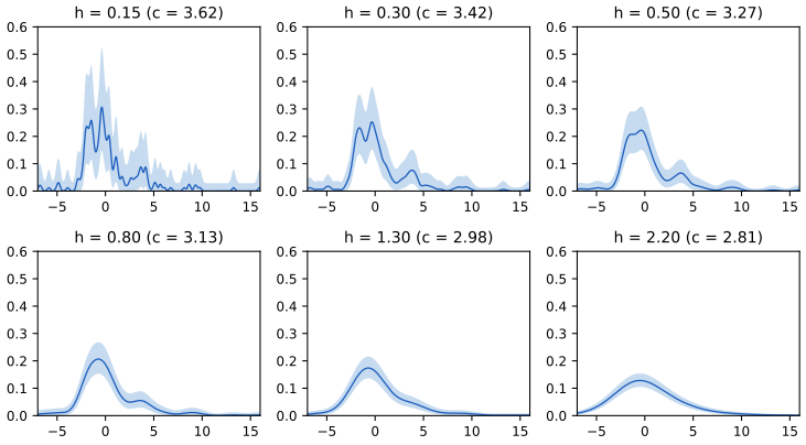
\[ \Big(\max\{\sqrt{\fh(x)}-cs,0\}\Big)^2\le\fb(x)\le\Big(\sqrt{\fh(x)}+cs\Big)^2\quad\text{for all }x\in[a,b] \]holds with probability about \(1-\alpha\). It is approximate on three counts (the delta method, the stationarity, and the Normal approximation in the tails), and, like every band of this chapter, it covers the smoothed \(\fb\), not \(f\). In 300 simulated Bart Simpson samples (\(n=1000\), \(h=0.05\), \(\kappa_0=84.9\), \(c=3.55\)) it covered \(\fb\) on \([-3,3]\) 96 percent of the time. Figures 6.S6 and 6.S7 apply it to the glass data. ∎
6.4 Local Polynomials
pp. 137–138 Kernel density estimators have boundary bias, as kernel regression does (Section 5.4). The density analogue of local polynomial regression is local likelihood (Loader 1999a; Hjort and Jones 1996). Generalise the log-likelihood to
\[ \mathcal L(f)=\sum_{i=1}^n\log f(X_i)-n\Big(\int f(u)\,\d u-1\Big), \]whose second term vanishes for densities and lets us maximise over all non-negative \(f\) without imposing \(\int f=1\).
Definitions 6.39 and 6.44 (local likelihood density estimate) pp. 137–138
The local log-likelihood at \(x\) is
\[ \mathcal L_x(f)=\sum_{i=1}^nK\Big(\frac{X_i-x}h\Big)\log f(X_i)-n\int K\Big(\frac{u-x}h\Big)f(u)\,\d u. \tag{6.40} \]Approximate \(\log f(u)\approx P_x(a,u)\) near \(x\), with
\[ \log f(u)\approx P_x(a,u),\tag{6.41} \] \[ P_x(a,u)=a_0+a_1(x-u)+\dots+a_p\frac{(x-u)^p}{p!}, \tag{6.42} \]so that
\[ \mathcal L_x(a)=\sum_{i=1}^nK\Big(\frac{X_i-x}h\Big)P_x(a,X_i)-n\int K\Big(\frac{u-x}h\Big)e^{P_x(a,u)}\,\d u . \tag{6.43} \]If \(\hat a\) maximises \(\mathcal L_x(a)\), the estimate is
\[ \fh(x)=e^{P_x(\hat a,x)}=e^{\hat a_0}. \tag{6.45} \]Filling the gap 6.14: degree 0 is the kernel estimator (Remark 6.46, Exercise 8), the general equations, and how to compute them p. 138
Derivation
Degree 0. With \(P_x=a_0\), \(\int K((u-x)/h)\,\d u=h\), and \(S_0=\sum_iK((X_i-x)/h)\),
\[ \mathcal L_x(a_0)=a_0S_0-nh\,e^{a_0},\qquad \frac{\d\mathcal L_x}{\d a_0}=S_0-nhe^{a_0}=0\iff e^{\hat a_0}=\frac{S_0}{nh}=\fh(x)\text{ of (6.26)}. \]The second derivative \(-nhe^{a_0}\lt0\), so this is the maximum.
Any degree: concavity and moment matching. \(\mathcal L_x\) is linear in \(a\) minus the integral of \(K\) times \(e^{\text{linear in }a}\), which is convex in \(a\); so \(\mathcal L_x\) is concave and the maximiser is unique when it exists. Setting the gradient to zero gives, for \(k=0,\dots,p\),
\[ \sum_iK\Big(\frac{X_i-x}h\Big)\frac{(x-X_i)^k}{k!}=n\int K\Big(\frac{u-x}h\Big)\frac{(x-u)^k}{k!}e^{P_x(\hat a,u)}\,\d u : \]the fitted local density reproduces the kernel-weighted empirical moments of orders \(0,\dots,p\) around \(x\). For \(p\ge1\) this corrects the boundary and slope bias in the same way local linear regression does.
Computation with a Gaussian kernel. Write \(t=(u-x)/h\) and the polynomial as \(b_0+b_1t+b_2t^2/2\) (the sign convention \((x-u)\) of (6.42) only flips \(b_1\)). Then
\[ \int\phi(t)e^{b_0+b_1t+b_2t^2/2}\d t=e^{b_0}\,\frac{1}{\sqrt{1-b_2}}\exp\Big(\frac{b_1^2}{2(1-b_2)}\Big)\quad(b_2\lt1), \]the normaliser of a \(N(\mu,s^2)\) density with \(s^2=1/(1-b_2)\), \(\mu=b_1s^2\); the gradient and Hessian are moments of that Normal. So Newton's method needs no numerical integration. The code's results agree with a direct numerical maximisation of (6.43). ∎
See also: local likelihood for regression in Chapter 5, Section 5.10.
6.5 Multivariate Problems
pp. 138–139 For \(X_i\in\R^d\) the usual choice is the product kernel
\[ \fh(x)=\frac1{nh_1\cdots h_d}\sum_{i=1}^n\Big\{\prod_{j=1}^dK\Big(\frac{x_j-X_{ij}}{h_j}\Big)\Big\}, \tag{6.47} \]with risk
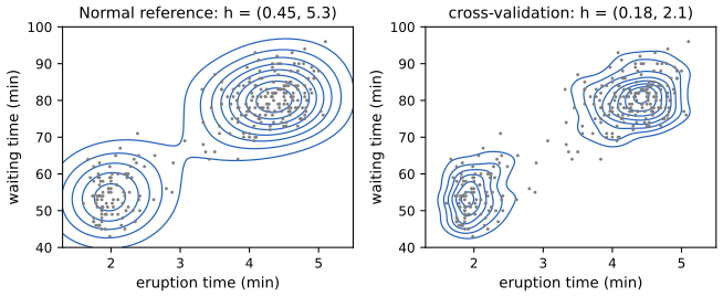
\[ R\approx\tfrac14\sigma_K^4\Big[\sum_{j=1}^dh_j^4\int f_{jj}^2(x)\,\d x+\sum_{j\ne k}h_j^2h_k^2\int f_{jj}f_{kk}\,\d x\Big]+\frac{\big(\int K^2\big)^d}{nh_1\cdots h_d}, \tag{6.48} \]\(f_{jj}\) being the second partial derivatives. The optimal bandwidths are \(h_j=O(n^{-1/(4+d)})\) and the risk \(O(n^{-4/(4+d)})\).
Filling the gap 6.15: (6.48), the rate \(n^{-4/(4+d)}\), and Silverman's table recomputed exactly pp. 138–139
Derivation
Bias. With \(u_j=(x_j-t_j)/h_j\), \(\E\fh(x)=\int\prod_jK(u_j)f(x-h\odot u)\,\d u\). A second-order Taylor expansion of \(f\) at \(x\): the constant gives \(f(x)\); first-order terms vanish since \(\int uK=0\); among the second-order terms \(\frac12\sum_{j,k}h_jh_ku_ju_kf_{jk}(x)\), the cross terms \(j\ne k\) vanish by independence of the coordinates under the product kernel, leaving \(b(x)=\frac12\sigma_K^2\sum_jh_j^2f_{jj}(x)+o(\max h_j^2)\). Squaring and integrating gives the bracket of (6.48): the diagonal of \((\sum_jh_j^2f_{jj})^2\) and its cross terms.
Variance. \(\V\fh(x)=\frac1n\V\big[\prod_jK_{h_j}(x_j-X_j)\big]\approx\frac{f(x)(\int K^2)^d}{nh_1\cdots h_d}\), and integrating gives the last term.
Rate. With all \(h_j=h\), \(R\approx C_1h^4+C_2/(nh^d)\), minimised at \(h\propto n^{-1/(d+4)}\) with \(R\propto n^{-4/(d+4)}\). To halve the risk, \(n\) must grow by the factor \(2^{(d+4)/4}\): 2.4 in one dimension, 5.7 in ten.
The table. For \(f=N(0,I_d)\) and a Gaussian product kernel with common \(h\), everything is Gaussian: \(\E\fh(0)=(2\pi(1+h^2))^{-d/2}\) and \(\E K_h(X)^2=(4\pi h^2)^{-d/2}(2\pi(1+h^2/2))^{-d/2}\), so the mean squared error at 0 is exact. Minimising it over \(h\) and finding the smallest \(n\) with relative MSE (MSE\(/f(0)^2\)) at most 0.1 gives
| \(d\) | 1 | 2 | 3 | 4 | 5 | 6 | 7 | 8 | 9 | 10 |
|---|---|---|---|---|---|---|---|---|---|---|
| book | 4 | 19 | 67 | 223 | 768 | 2790 | 10,700 | 43,700 | 187,000 | 842,000 |
| exact | 4 | 19 | 67 | 223 | 768 | 2788 | 10,730 | 43,684 | 187,275 | 841,566 |
The table (Silverman 1986) is reproduced to its printed precision. ∎
A density estimate in many dimensions should never be reported without a band; the bands are wide, and correctly so: the difficulty is in the problem, not in the method.
See also: Chapter 4, Filling the gap 4.6 (the curse of dimensionality) and, in the companion course, Probability and Statistical Inference, Filling the gap 20.13.
6.6 Converting Density Estimation Into Regression
pp. 139–140 An old idea, made rigorous by Nussbaum (1996a) and Brown et al. (2005): bin the data finely and treat the root counts as regression data. For data on \([0,1]\), take \(k\approx n/10\) equal bins with counts \(N_j\) and midpoints \(t_j\), and set
\[ Y_j=\sqrt{\frac kn}\times\sqrt{N_j+\frac14}. \tag{6.49} \]Then
\[ Y_j\approx r(t_j)+\sigma\epsilon_j,\qquad \epsilon_j\sim N(0,1),\quad\sigma=\sqrt{\frac k{4n}},\quad r(x)=\sqrt{f(x)}. \tag{6.50} \]Any regression smoother gives \(\hat r_n\), and
\[ \fh(x)=\frac{(\hat r_n^+(x))^2}{\int_0^1(\hat r_n^+(s))^2\,\d s},\qquad \hat r_n^+=\max\{\hat r_n,0\}. \]On an interval of length \(\ell\) replace \(k\) by \(k/\ell\) (bins per unit length). Binning is not the smoothing step: the regression smoother is.
Filling the gap 6.16: why (6.50) holds, why \(1/4\), and what the known \(\sigma\) buys pp. 139–140
Derivation
Counts are nearly Poisson. \(N_j\sim\text{Binomial}(n,p_j)\) with \(p_j=\int_{B_j}f=f(t_j)/k+O(k^{-3})\) (the midpoint rule, for \(f''\) bounded). With \(\lambda_j=np_j\approx nf(t_j)/k\), \(\E N_j=\lambda_j\) and \(\V N_j=\lambda_j(1-p_j)\approx\lambda_j\) since \(p_j=O(1/k)\).
The square root, to second order. Let \(N\) have mean \(\lambda\), \(\E(N-\lambda)^2=\lambda\), \(\E(N-\lambda)^3=\lambda\) (Poisson). Expanding \(\sqrt{\lambda+c+D}\), \(D=N-\lambda\), in powers of \((c+D)/\lambda\) and taking expectations,
\[ \E\sqrt{N+c}=\sqrt\lambda+\frac{4c-1}{8\sqrt\lambda}+O(\lambda^{-3/2}),\qquad \V\sqrt{N+c}=\frac14+\frac{3-8c}{32\lambda}+O(\lambda^{-2}). \]So \(c=\frac14\) removes the \(\lambda^{-1/2}\) bias of the mean (the choice of (6.49)), with variance \(\frac14+\frac1{32\lambda}\); \(c=\frac38\) (Anscombe 1948) is the choice that makes the variance \(\frac14+O(\lambda^{-2})\). Both expansions were confirmed numerically with exact Poisson sums.
Rescaling. Multiplying by \(\sqrt{k/n}\): \(\E Y_j\approx\sqrt{k/n}\sqrt{nf(t_j)/k}=\sqrt{f(t_j)}\) and \(\V Y_j\approx\frac kn\cdot\frac14=\frac k{4n}\). The \(Y_j\) are nearly independent (multinomial counts have correlations of order \(1/k\)) and nearly Normal when \(\lambda_j\) is not small. That is (6.50): equally spaced design, constant and known variance.
What the known \(\sigma\) buys. (1) The band of Chapter 5 needs no variance estimate: \(\hat r_n(x)\pm c\,\sigma\|\bl(x)\|\) with \(c\) from the tube formula (5.102). Squaring is increasing on \([0,\infty)\), so if \(\bar r\in[\ell,u]\) then \(\bar r^2\in[(\ell^+)^2,(u^+)^2]\); dividing by the normalising constant adds a small extra error that the book ignores. (2) The risk of the linear smoother can be estimated without bias: \(\E\|Y-LY\|^2=\|(I-L)r\|^2+\sigma^2(k-2\tr L+\tr L^\T L)\) gives
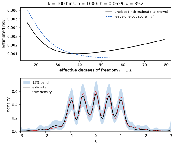
\[ C_p(h)=\frac1k\|Y-LY\|^2-\sigma^2+\frac{2\sigma^2\tr L}k,\qquad\E C_p=\frac1k\E\|LY-r\|^2 \](Mallows' \(C_p\), Section 5.3). In the example below the leave-one-out score is nearly flat for small bandwidths and is minimised at the smallest bandwidth considered, while \(C_p\) has a clear minimum. ∎
Example 6.51. Figure 6.6 applies the method to the 1000 Bart Simpson draws, with \(k=100\) bins on \([-3,3]\) and local linear regression with a Gaussian kernel. The book selects the bandwidth by cross-validation and finds a minimum near 40 effective degrees of freedom. For this sample the leave-one-out score keeps decreasing as \(h\) shrinks (it nearly interpolates the root counts), while the unbiased risk estimate, which uses the known \(\sigma=0.0645\), is minimised at \(h=0.063\), \(\nu=39.2\): the region of the book's minimum. The tube formula gives \(\kappa_0=67.6\) and \(c=3.49\).
6.7 Bibliographic Remarks
Kernel density estimation goes back to Rosenblatt (1956) and Parzen (1962); least-squares cross-validation to Rudemo (1982). Scott (1992) and Silverman (1986) are the standard books. The scale-space view (SiZer, Section 5.11) is in Chaudhuri and Marron (1999, 2000).
6.8 Appendix
The appendix proves Theorem 6.11; the full argument, with the exact risk formula and the correction of the variance remainder, is Filling the gap 6.3.
Notes on the book
The book's website has no errata list. Each point below gives the evidence: a derivation in these notes or a computation.
Page 128, Example 6.8: "oversmoothing" and "undersmoothing" are swapped
The text says the top left histogram "has too many bins resulting in oversmoothing and too much bias" and the bottom left "has too few bins resulting in undersmoothing". Too many bins is undersmoothing, with too much variance; too few bins is oversmoothing, with too much bias. The figure's own panel labels (Undersmoothed top left, Oversmoothed bottom left) are right. Also, the cross-validated number of bins for the 1266 redshifts below 0.2 on \([0,0.2]\) is 258, not 308; the score is so flat that 308 is within 3 percent of the minimum (Figure 4.1).
Page 129, (6.12), and page 142: the variance remainder is \(-\int f^2/n+o(1/n)\), not \(o(1/n)\)
The last line of the appendix proof turns \(\frac1{nh}-\frac1n(\int f^2+o(1))\) into \(\frac1{nh}+o(\frac1n)\); the term \(-\frac1n\int f^2\) is of order \(1/n\) exactly. The exact risk formula of Filling the gap 6.3 shows it, and Figure 6.S1 (right) confirms that \(n\times\)(exact risk minus (6.12)) tends to \(-\int f^2=-1.2\) for the Beta(2,2) density. The optimal width and the \(n^{-2/3}\) rate are unaffected.
Page 130, proof of Theorem 6.20: \(\sqrt{\fb}\) in place of \(\sqrt f\)
The event \(A\) is written as \(\max_x|\sqrt{\fh(x)}-\sqrt{f(x)}|\le c\); it should be \(\sqrt{\fb(x)}\), the target of the band (6.19). With \(\sqrt f\) the following equality with \(\max_j2\sqrt n|\sqrt{\ph_j}-\sqrt{p_j}|\) would be false. The theorem also needs \(f\) bounded away from 0 on the support (or at least that every bin holds many points): Figure 6.S2 shows the coverage failing on \([-3,3]\) for the Bart Simpson density, where the tails are nearly empty. See Filling the gap 6.5, which also notes that a rigorous version uses \(m(\log m)^3/n\to0\).
Page 136, (6.35): the remainder is \(O(1/n)\), not \(O(1/n^2)\)
Replacing \(\frac1{n(n-1)}\) by \(\frac1{n^2}\) in the leave-one-out term leaves \(-\frac2{n^2(n-1)h}\sum_{i\ne j}K((X_i-X_j)/h)\), whose mean is \(-\frac2n\int\fb f\approx-\frac2n\int f^2\) (Filling the gap 6.11). On the galaxy data at the cross-validated bandwidth this remainder equals \(-29.9/n\). It depends on \(h\) only weakly, which is why (6.35) still gives nearly the right bandwidth.
Page 137, a typo
"maximize over all non-negative \(f\) with imposing the constraint" should read "without imposing the constraint" \(\int f=1\): that is the purpose of the extra term \(-n(\int f-1)\).
Page 141, Figure 6.6: the selector
The book's top panel shows a cross-validation score with a minimum near 40 degrees of freedom. On our sample of 1000 draws the leave-one-out score has no interior minimum (it decreases down to the smallest bandwidth on the grid), but the unbiased risk estimate that the known \(\sigma\) of (6.50) makes available is minimised at \(\nu=39.2\). On three other simulated samples, leave-one-out picked between 37 and 61 degrees of freedom while \(C_p\) picked 37 to 40 every time. This is not an error of the book (it depends on the sample), but a reason to prefer \(C_p\) in this setting (Filling the gap 6.16).
6.9 Exercises
Exercise 6.1. Prove Theorem 6.27.
Solution
See Filling the gap 6.6: the bias \(\int K(u)\{f(x-hu)-f(x)\}\d u\to0\) by continuity at \(x\) (split the integral at \(|u|\lt\delta/h\)), and the variance is at most \(\|K\|_\infty\|f\|_\infty/(nh)\to0\); Chebyshev's inequality concludes.
Exercise 6.2. For the boxcar kernel \(K(x)=1\) on \((-\frac12,\frac12)\) and 0 otherwise, show (a) \(\E\fh(x)=\frac1h\int_{x-h/2}^{x+h/2}f(y)\,\d y\) and \(\V\fh(x)=\frac1{nh^2}\big[\int_{x-h/2}^{x+h/2}f-\big(\int_{x-h/2}^{x+h/2}f\big)^2\big]\); (b) if \(h\to0\) and \(nh\to\infty\) then \(\fh(x)\overset P\to f(x)\).
Solution
(a) Here \(\fh(x)=\frac1{nh}N\) with \(N=\#\{i:|X_i-x|\lt h/2\}\sim\text{Binomial}(n,P)\), \(P=\int_{x-h/2}^{x+h/2}f\). So \(\E\fh(x)=P/h\) and \(\V\fh(x)=nP(1-P)/(nh)^2=(P-P^2)/(nh^2)\), the two formulas. (b) At a point where \(f\) is continuous (or any Lebesgue point), \(P/h\to f(x)\) as \(h\to0\), so the bias tends to 0; the variance is at most \(\frac{P}{h}\cdot\frac1{nh}\to f(x)\cdot0=0\). Chebyshev's inequality gives consistency. Both moment formulas were confirmed by simulation with the Bart Simpson density.
Exercise 6.3. Prove that \(\hJ(h)\) is an unbiased estimate of \(\E J(h)\) for histograms and kernel density estimates.
Solution
General argument in Filling the gap 6.1: conditioning on the other observations, \(\E\hat f_{(-i)}(X_i)=\E\int\hat f_{n-1}f\), and for both estimators \(\E\hat f_m(x)\) does not depend on \(m\). A direct verification for the histogram, computing both sides in closed form, ends Filling the gap 6.4.
Exercise 6.4. Prove equation (6.35).
Solution
See Filling the gap 6.11. The exact score is \(\frac1{n^2h}\sum_{i,j}K^{(2)}-\frac2{n(n-1)h}\sum_{i\ne j}K\); splitting \(\frac1{n(n-1)}=\frac1{n^2}+\frac1{n^2(n-1)}\) and adding back the diagonal gives (6.35) with remainder \(-\frac2{n^2(n-1)h}\sum_{i\ne j}K\), which is of order \(1/n\) (note).
Exercise 6.5. Study the distribution of the salaries of the chief executive officers of 60 companies with a histogram and a kernel estimator (least-squares cross-validation, and the Normal reference rule), decide with confidence bands whether its bumps are real, and try several kernel shapes.
Solution
Data. The address given in the book (the DASL archive at lib.stat.cmu.edu) no longer serves the file, and the data are not on the book's website, so the exercise cannot be reproduced exactly. The method is the one of Exercise 6, and the code runs it on any vector of salaries:
hist_cv_curveandhist_bandfor the histogram,kde_hcvwithkind="gauss","epan"or"boxcar",normal_reference_h, andkde_bandfor a band.What to expect and how to judge the bumps. Salaries are strongly right-skewed, so the Normal reference rule (driven by \(\min\{s,Q/1.34\}\)) gives a moderate bandwidth and the cross-validated one is usually smaller. With \(n=60\) the bands are wide (the square-root half-width \(c\sqrt{R(K)/(4nh)}\) is large), and a bump is credible only if the band rules out every unimodal shape there: the upper limit at the dip must lie below the lower limit at both neighbouring peaks. With 60 observations that is rarely the case. Analysing \(\log(\text{salary})\) and transforming back is often better for skewed data, since one bandwidth then suits both the bulk and the tail.
Exercise 6.6. For the glass fragments data, estimate the density of the refractive index by a histogram and a kernel estimator, with cross-validation, different binwidths, bandwidths and kernels, and 95 percent bands.
Solution
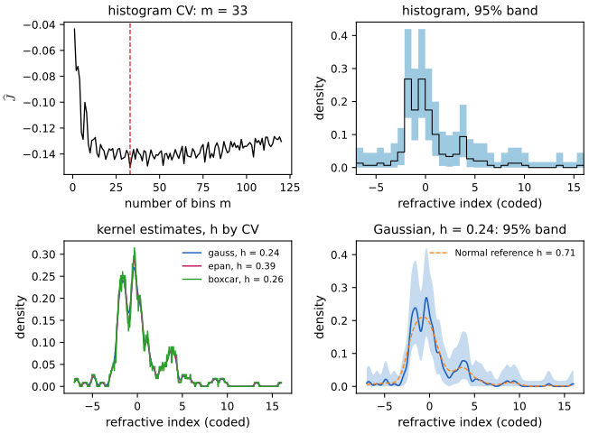
Data: the 214 values of RI (coded refractive index), from \(-6.85\) to 15.93; histograms on \([-7,16]\). Results (Figure 6.S6):
estimator smoothing parameter chosen by histogram m = 33 (width 0.70) score (6.16) Gaussian kernel h = 0.240 exact score (6.33) Epanechnikov kernel h = 0.385 exact score boxcar kernel h = 0.260 exact score Gaussian kernel h = 0.713 Normal reference rule The three kernel estimates with cross-validated bandwidths are almost indistinguishable once each kernel's scale is taken into account (\(\sigma_K=1\), 0.447 and 0.577: the effective widths are 0.24, 0.17 and 0.15): the kernel shape hardly matters. The histogram score is very flat beyond 20 bins. Both estimators show a main mode between about \(-2\) and 0.5 (the cross-validated kernel estimate splits it into two peaks near \(-1.5\) and \(-0.3\)), a shoulder or small bump near 4, and a long right tail with isolated values up to 16. The Normal reference rule, three times wider than cross-validation, merges the two peaks. Bands: the histogram band (6.21) with \(m=33\), and the kernel band of Filling the gap 6.13 for \(h=0.24\) (\(\kappa_0=67.8\), \(c=3.49\)). Both bands rule out a density near 0 on the main mode, but neither can separate the two peaks of the main mode, nor establish the bump near 4 (see Exercise 7).
Exercise 6.7. For the same data, examine the fit as a function of the bandwidth, plotting fits with bands for many values of \(h\) (optionally, with the method of Chaudhuri and Marron 1999).
Solution
Figure 6.S7 shows the Gaussian kernel estimate with its 95 percent band for \(h=0.15,\ 0.3,\ 0.5,\ 0.8,\ 1.3,\ 2.2\); the constant \(c\) falls from 3.62 to 2.81 as \(h\) grows, because \(\kappa_0\propto1/h\). The main mode is significant at every scale. The bump near 4 is visible for \(h\) from about 0.24 to 0.8, but at no bandwidth does the band exclude a monotone decline from the main mode: at \(h=0.5\), for instance, the upper limit in the dip near 2.3 is 0.078, above the lower limit 0.030 at the bump near 3.7. So the data do not establish that bump. This is the logic of SiZer (Chaudhuri and Marron 1999), applied to the density rather than its derivative; the regression version of the SiZer map for these data is in Chapter 5, Section 5.11.
Exercise 6.8. Prove that local likelihood density estimation reduces to kernel density estimation when \(p=0\).
Solution
With \(P_x=a_0\), (6.43) is \(a_0\sum_iK((X_i-x)/h)-nhe^{a_0}\), maximised at \(e^{\hat a_0}=\frac1{nh}\sum_iK((X_i-x)/h)\), which is (6.26). Details in Filling the gap 6.14; the code's degree-0 estimate equals the kernel estimate to rounding.
Exercise 6.9. Apply local polynomial density estimation to the data of Exercise 6.
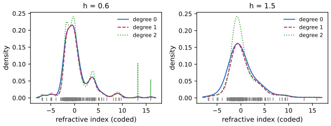
Solution
Figure 6.S4: Gaussian kernel, degrees 0, 1, 2, with \(h=0.6\) and \(h=1.5\), computed by Newton's method on the concave local log-likelihood with the closed-form Gaussian integrals of Filling the gap 6.14. At \(h=0.6\) degrees 0 and 1 agree closely; degree 2 sharpens the main peak (0.24 instead of 0.21) but fits narrow spikes at the isolated points near 13 and 16. At \(h=1.5\) degree 0 flattens the mode to 0.16 while degree 2 keeps it at 0.24: higher degree reduces the bias of a wide window, at the price of variance where data are sparse. A moderate degree (1) with a moderate bandwidth is the safe choice here.
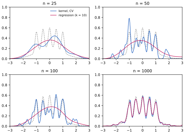
Exercise 6.10. Generate data from the Bart Simpson distribution (6.2) and compare kernel density estimation with the method of Section 6.6, for \(n=25,50,100,1000\).
Solution
Method: 100 samples for each \(n\). Kernel estimator: Gaussian kernel, \(h\) by the exact score (6.33). Regression method: \(k=\max(\text{round}(n/10),10)\) bins on \([-3,3]\), local linear regression with \(h\) by \(C_p\), squared and normalised. Integrated squared error over \([-3,3]\):
n kernel, mean ISE regression, mean ISE regression better in 25 0.081 0.065 68% 50 0.064 0.057 66% 100 0.046 0.054 21% 1000 0.0069 0.0078 24% For \(n\le50\) neither method can see the claws, and the regression method, with its few wide bins, gives a steadier smooth hump. From \(n=100\) the kernel estimator starts to resolve the claws while the bins of width 0.6 cannot, so it wins; at \(n=1000\) both resolve them (Figure 6.S8) and the kernel estimator is about 10 percent better. The regression method's advantage is not accuracy but inference: it comes with a band.
Demonstrations for this chapter
| Demonstration | What you can see | Sections and results |
|---|---|---|
| Histograms: cross-validation and a confidence band | Histograms of the galaxy, Bart Simpson and glass data for any number of bins, the closed-form score (6.16), the band (6.21) at three levels, and a coverage simulation. Presets: 1 the CV choice (Fig 6.2); 2 too many bins; 3 too few bins; 4 the band (Fig 6.3); 5 coverage on the Bart Simpson density. | 6.2; Theorems 6.15, 6.20; Filling the gaps 6.4, 6.5 |
| Kernel density estimation: bandwidth, cross-validation and a band | Three kernels on three data sets; the exact score (6.33) against \(h\), the Normal reference rule, the integrated squared error against the true Bart Simpson density, and the square-root band. Presets: 1 h by CV (Fig 6.1); 2 h/10; 3 10h; 4 the Normal reference rule on the claw; 5 galaxies with a band (Fig 6.5). | 6.3; Theorems 6.28, 6.34; Filling the gaps 6.9, 6.11, 6.13 |
| Density estimation as regression on root counts | Binning, the root transform, local linear regression with \(C_p\) or leave-one-out, the tube band, and the comparison with the kernel estimator for \(n=25\) to 1000. Presets: 1 Figure 6.6; 2 the leave-one-out choice; 3 n = 100; 4 n = 25; 5 too many bins. | 6.6; Filling the gap 6.16; Exercise 10 |
Related demonstrations in the companion courses: histogram cross-validation and histogram or kernel: the two rates (Probability and Statistical Inference), kernel density bandwidth (Statistical Learning), density estimation (Bayesian and Probabilistic Machine Learning). The Python code that produces every figure of this page is code/ch06_density_estimation.py (see the code index).
References
- Anscombe, F. J. (1948). The transformation of Poisson, binomial and negative-binomial data. Biometrika, 35, 246–254.
- Brown, L. D., Carter, A. V., Low, M. G. and Zhang, C.-H. (2004). Equivalence theory for density estimation, Poisson processes and Gaussian white noise with drift. Annals of Statistics, 32, 2074–2097 (cited by the book as Brown et al. 2005).
- Chaudhuri, P. and Marron, J. S. (1999). SiZer for exploration of structures in curves. Journal of the American Statistical Association, 94, 807–823.
- Chaudhuri, P. and Marron, J. S. (2000). Scale space view of curve estimation. Annals of Statistics, 28, 408–428.
- Hall, P. and Marron, J. S. (1987). Extent to which least-squares cross-validation minimises integrated square error in nonparametric density estimation. Probability Theory and Related Fields, 74, 567–581.
- Hjort, N. L. and Jones, M. C. (1996). Locally parametric nonparametric density estimation. Annals of Statistics, 24, 1619–1647.
- Loader, C. (1999a). Local Regression and Likelihood. Springer, New York.
- Loader, C. (1999b). Bandwidth selection: classical or plug-in? Annals of Statistics, 27, 415–438.
- Marron, J. S. and Wand, M. P. (1992). Exact mean integrated squared error. Annals of Statistics, 20, 712–736.
- Nussbaum, M. (1996). Asymptotic equivalence of density estimation and Gaussian white noise. Annals of Statistics, 24, 2399–2430.
- Parzen, E. (1962). On estimation of a probability density function and mode. Annals of Mathematical Statistics, 33, 1065–1076.
- Petrov, V. V. (1975). Sums of Independent Random Variables. Springer, Berlin.
- Rosenblatt, M. (1956). Remarks on some nonparametric estimates of a density function. Annals of Mathematical Statistics, 27, 832–837.
- Rudemo, M. (1982). Empirical choice of histograms and kernel density estimators. Scandinavian Journal of Statistics, 9, 65–78.
- Scott, D. W. (1992). Multivariate Density Estimation. Wiley, New York.
- Silverman, B. W. (1986). Density Estimation for Statistics and Data Analysis. Chapman and Hall, London.
- Stone, C. J. (1984). An asymptotically optimal window selection rule for kernel density estimates. Annals of Statistics, 12, 1285–1297.
- Tsybakov, A. B. (2009). Introduction to Nonparametric Estimation. Springer, New York (Assouad's lemma, Chapter 2).
- van der Vaart, A. W. (1998). Asymptotic Statistics. Cambridge University Press.
The numerical statements in the text (the closed-form scores against their definitions, the unbiasedness identities, the exact risk formulas, the band coverages, the Silverman table, the local likelihood fits, the root-transform expansions, and the numbers of the examples and exercises) were confirmed numerically.