Generative Adversarial Networks
A generator network turns random noise into samples; a discriminator network tries to tell those samples from real data; each is trained against the other. Because the generator never needs a likelihood, it can be any differentiable map, and the discriminator supplies the training signal that a likelihood would otherwise provide. Section 17.1 sets up the game, shows that with unlimited capacity its solution is the data distribution, and explains why training it is hard: the gradients can vanish, the game can cycle, and the generator can collapse onto a few modes. The remedies (a non-saturating loss, least squares, Wasserstein distances) each come from a different way of measuring how far apart two distributions are. Section 17.2 looks at image GANs, their latent spaces and CycleGAN, which learns to translate between two collections of images without paired examples.
Ch. 1 Deep learning revolution Ch. 2 Probabilities Ch. 3 Standard distributions Ch. 4 Regression Ch. 5 Classification Ch. 6 Deep neural networks Ch. 7 Gradient descent Ch. 8 Backpropagation Ch. 9 Regularization Ch. 10 Convolutional networks Ch. 11 Structured distributions Ch. 12 Transformers Ch. 13 Graph neural networks Ch. 14 Sampling Ch. 15 Discrete latent variables Ch. 16 Continuous latent variables Ch. 17 GANs Ch. 18 Normalizing flows Ch. 19 Autoencoders Ch. 20 Diffusion models Appendices A to C
How to read these notes
They follow the book. Sections carry the book's numbers (17.1, 17.1.2, ...) and every displayed equation that appears in the book carries the book's own equation number, e.g. (17.15). Equations without a number are steps that the book skips.
Filling the gaps. The chapter is short and states most of its theory in words or leaves it to the exercises. Wherever it says a result "can be shown", gives an argument informally, or leaves it out, an orange Filling the gap box or a proof gives the full argument. Proofs start hidden: open one with its bar, or use the button below. Every numerical claim has been confirmed by computation.
Figures and demonstrations. Of the ten figures, five are computed here: Figures 17.2 and 17.3 directly, and Figures 17.6, 17.9 and 17.10 (which show large published models) at small scale, with two-dimensional data and MNIST digits. The other five are diagrams of architectures and information flow and are not reproduced. Eight supplementary figures (17.S1 to 17.S8, our own) illustrate the gaps that are filled. The ▶ Demo boxes open an interactive demonstration already set to the case being discussed.
Main reference
C. M. Bishop and H. Bishop, Deep Learning: Foundations and Concepts, Springer (2024), Chapter 17, pages 533–545. Section, equation, figure and exercise numbers below refer to this book. Further reading is listed in the references; the book's website is www.bishopbook.com. There is no official solution for the exercises of this chapter; all solutions below are my own.
The explanations, derivations, figures and code are my own; equations are cited by their numbers in the book.
Companion course: Bayesian and Probabilistic Machine Learning
GANs are not in Bishop (2006), so this chapter is treated in full here. The tools it uses are covered in the companion course Bayesian and Probabilistic Machine Learning, and its advanced module covers the other deep generative models with which GANs are usually compared.
- Relative entropy and Gibbs' inequality, used for the Jensen–Shannon form of the GAN objective: Section 1.6.1 and Result 1.22 (here Result 17.2); the median as the minimiser of an absolute (L1) error, which explains the L1 cycle loss: Result 1.19 (here Result 17.12).
- Logistic sigmoid outputs and the cross-entropy error that the discriminator minimises: Section 4.3.2 (here 17.1.1); network training and backpropagation: Sections 5.2 and 5.3.
- Variational calculus for the optimal discriminator: toolkit, calculus of variations; why minimising KL(q‖p) is mode seeking: Section 10.1.2 (here Result 17.7).
- Nonlinear latent variable models: Section 12.4; mixtures of Gaussians, the data of the ring experiments: Section 9.2.
- The other deep generative models, with likelihoods: Advanced topics: deep generative models, namely variational autoencoders, normalizing flows, autoregressive models and diffusion models (here Filling the gap 17.1).
- Demonstrations: backpropagation, a VAE's latent space, a normalizing flow, a diffusion model.
The chapter at a glance
- 17.1.1 For a fixed generator the best discriminator is \(d^\star=\pd/(\pd+\pG)\) (Result 17.1); at that discriminator the error equals \(\ln4-2\JS(\pd,\pG)\), so the generator's best move is \(\pG=\pd\) (Result 17.2). This is a statement about the solution, not about gradient training: on the bilinear game of Exercise 17.2, simultaneous gradient steps spiral away from it, alternating steps cycle, and only a corrected method converges (Result 17.3).
- 17.1.2 Against a fixed discriminator the generator's best response is a point mass, which is mode collapse (Result 17.5). When the two distributions barely overlap, the optimal discriminator is a step and the minimax loss passes almost no gradient (Figure 17.2, Filling the gap 17.4); instance noise, least squares (Result 17.6) and the non-saturating loss (Result 17.7, a reverse KL in disguise) each restore it differently. The Wasserstein distance keeps measuring how far apart distributions are when JS cannot (Results 17.8–17.11).
- 17.2 Convolutional generators, smooth latent spaces and latent arithmetic (Figures 17.9 and 17.10, reproduced on MNIST); CycleGAN's cycle loss forces the two translators to be inverse bijections (Result 17.12). Since a GAN has no likelihood, it is evaluated by statistics of its samples (Result 17.13).
Notation. \(\pd\) is the data density and \(\pG\) the density of \(\bx=\bg(\bz,\bw)\) when \(\bz\sim p(\bz)\); when we write \(p\) and \(q\) for short, \(p=\pd\) and \(q=\pG\). \(d(\bx,\bphi)\in(0,1)\) is the discriminator, \(E\) the error it minimises and the generator maximises (17.6), \(d^\star\) the optimal discriminator, and \(M=(p+q)/2\). \(\JS\) is the Jensen–Shannon divergence (Definition 17.2), \(\W\) the Wasserstein-1 distance (Definition 17.3), \(\sigma\) the logistic sigmoid and \(a\) a logit, \(d=\sigma(a)\).
Printings. The first printing has a sign error in (17.17), which makes the "minimum" of Exercise 17.1 a maximum of the error as defined in (17.16); a garbled gradient-penalty error (17.11); and a misleading description of mode collapse. Each is flagged where it occurs, and the list with the evidence is in the summary before the exercises.
p. 533 A generative model learns a distribution \(p(\bx\given\bw)\) from training data and then produces new samples from it; a conditional generative model \(p(\bx\given\bc,\bw)\) does so given a label or other conditioning vector \(\bc\) (a cat rather than a dog). Autoregressive language models (Section 12.3) are one family. This chapter starts the second family: a nonlinear latent-variable model, in which a simple random vector \(\bz\) is pushed through a deep network. GANs are the first of four such models in the book; variational autoencoders, normalizing flows and diffusion models (Chapters 18 to 20) are the others, and the companion course's advanced module treats them in its own way.
17.1 Adversarial Training
p. 534 Take a latent distribution
\[ p(\bz)=\N(\bz\given\bzero,\bI) \tag{17.1} \]and a generator network \(\bx=\bg(\bz,\bw)\). Together they define a distribution \(\pG\) of \(\bx\) implicitly: we can sample from it (draw \(\bz\), apply \(\bg\)) but cannot evaluate its density, so the parameters \(\bw\) cannot be fitted by maximum likelihood. The idea of generative adversarial networks (Goodfellow et al., 2014) is to train a second network, the discriminator, to tell generated samples from data, and to use its output as the training signal for the generator (the book's Figure 17.1, a diagram of the two networks, is not reproduced).
Filling the gap 17.1: why an implicit model has no usable likelihood p. 534
The book says the likelihood "cannot, in general, be evaluated in closed form". In fact it often does not exist at all.
Derivation
Equal dimensions, invertible generator. If \(\bz\) and \(\bx\) both live in \(\R^D\) and \(\bg(\cdot,\bw)\) is a smooth bijection with a smooth inverse, the change-of-variables formula (Section 2.4) gives \(\pG(\bx)\)
Fewer latent than data dimensions. In image GANs \(\bz\in\R^M\) with \(M\) (about 100) far below \(D\) (thousands of pixels). Suppose \(\bg\) is Lipschitz with constant \(L\) (true for networks with Lipschitz activations and finite weights). Cover the cube \([-r,r]^M\) by \(n^M\) small cubes of side \(2r/n\); each has diameter \(2r\sqrt M/n\), so its image lies in a ball of radius \(2rL\sqrt M/n\), of volume \(c_D(2rL\sqrt M/n)^D\). The image of the big cube therefore has volume at most \(n^M c_D(2rL\sqrt M)^Dn^{-D}\to0\) as \(n\to\infty\), because \(M<D\). Taking \(r=1,2,\dots\) shows that \(\bg(\R^M)\) has Lebesgue measure zero in \(\R^D\): \(\pG\) is concentrated on a thin set and has no density. A data point off that set has likelihood zero, and a log likelihood of \(-\infty\) gives no gradient.
What a GAN needs instead. Only samples \(\bg(\bz,\bw)\) and the derivatives \(\partial\bg/\partial\bw\), both available from any network. The thin support has a price, which returns in Result 17.8: two such distributions almost never overlap, and divergences that compare densities point by point then stop being informative. ∎
17.1.1 Loss function
See also the companion course, logistic regression and the cross-entropy error (Section 4.3.2), and in this course Section 6.4.2 (binary classification error).
p. 535 Label real data and generated ("synthetic") data by a binary target,
\[ t=1,\quad\text{real data}, \tag{17.2} \] \[ t=0,\quad\text{synthetic data}. \tag{17.3} \]The discriminator has one logistic-sigmoid output, read as the probability that its input is real,
\[ P(t=1)=d(\bx,\bphi), \tag{17.4} \]and is trained with the cross-entropy error
\[ E(\bw,\bphi)=-\frac1N\sum_{n=1}^N\{t_n\ln d_n+(1-t_n)\ln(1-d_n)\}, \tag{17.5} \]where \(d_n=d(\bx_n,\bphi)\). The inputs are real examples \(\bx_n\) and synthetic ones \(\bg(\bz_n,\bw)\) with \(\bz_n\sim p(\bz)\); splitting the sum by label,
\[ E_{\rm GAN}(\bw,\bphi)=-\frac1{N_{\rm real}}\sum_{n\in\rm real}\ln d(\bx_n,\bphi)-\frac1{N_{\rm synth}}\sum_{n\in\rm synth}\ln\big(1-d(\bg(\bz_n,\bw),\bphi)\big). \tag{17.6} \]The discriminator minimises this error and the generator maximises it, by gradient steps of opposite sign on a mini-batch,
\[ \Delta\bphi=-\lambda\nabla_\bphi E_n(\bw,\bphi), \tag{17.7} \] \[ \Delta\bw=\lambda\nabla_\bw E_n(\bw,\bphi), \tag{17.8} \]p. 536 usually alternating one step of each and drawing new synthetic samples every time. When training is over, the discriminator is discarded and the generator samples by mapping fresh \(\bz\).
Definition 17.1 (the GAN game in function space) pp. 535–536; Exercise 17.1, (17.14)
Let \(p=\pd\) be the data density and \(q=\pG\) the generator's. With infinitely many samples, (17.6) becomes
\[ E(q,d)=-\int p(\bx)\ln d(\bx)\,\d\bx-\int q(\bx)\ln\big(1-d(\bx)\big)\,\d\bx . \tag{17.14} \]The discriminator chooses a function \(d:\R^D\to(0,1)\) to minimise \(E\); the generator chooses \(q\) (through \(\bw\)) to maximise it. Since one player's gain is the other's loss, this is a two-player zero-sum game. Goodfellow et al. (2014) write it with the opposite sign, as \(\min_G\max_D V\) with \(V=-E\); the two descriptions are the same game.
Filling the gap 17.2: from (17.5) to (17.6) and (17.14), and what the gradients are pp. 535–536
Derivation
Normalisation. With \(N=N_{\rm real}+N_{\rm synth}\), (17.5) is \(-\frac1N\sum_{\rm real}\ln d_n-\frac1N\sum_{\rm synth}\ln(1-d_n)\) because \(t_n\) kills one of the two terms. (17.6) normalises each group by its own size; for \(N_{\rm real}=N_{\rm synth}=N/2\) it is exactly twice (17.5), which changes no minimiser. With unequal group sizes (17.5) weights the two classes by \(\pi=N_{\rm real}/N\) and \(1-\pi\); (17.6) weights them equally, which is what makes \(d^\star\) in Result 17.1 independent of the batch composition.
Population limit. Each average in (17.6) is a Monte Carlo estimate (Section 14.1.1): \(\frac1{N_{\rm real}}\sum\ln d(\bx_n)\)
Gradients. \(\nabla_\bphi\) acts on \(d\) only, so the mini-batch gradient is an unbiased estimate of \(\nabla_\bphi E\). For \(\bw\) the expectation is over \(q\), which depends on \(\bw\); writing it over \(\bz\) instead, \(\E_q[\ln(1-d(\bx))]\)
This is the reparameterisation estimator of Filling the gap 14.2: the generator learns only through the input gradient \(\nabla_\bx d\) of the discriminator at its samples, a fact that drives everything in Section 17.1.2. In code, backpropagation runs through the discriminator into the generator; the discriminator's weights are simply not updated in that step.
Simultaneous and alternating steps. (17.7)–(17.8) taken together are gradient descent–ascent. "Simultaneous" evaluates both gradients at the same \((\bw,\bphi)\); "alternating" (the book's recipe, and the demos') updates \(\bphi\) first and then evaluates \(\nabla_\bw\) at the new \(\bphi\). Result 17.3 shows that the difference matters. ∎
p. 536 If the generator becomes perfect the discriminator cannot do better than guessing and outputs 1/2 everywhere. The book states that with unlimited flexibility a fully optimised GAN reproduces the data distribution exactly (Exercise 17.1); the next two results prove it.
Result 17.1 (the optimal discriminator) (17.15); Exercise 17.1
Let \(p\) and \(q\) be densities (with respect to a common measure). For fixed \(q\), the discriminator that minimises (17.14) over all functions \(d\) is
\[ d^\star(\bx)=\frac{\pd(\bx)}{\pd(\bx)+\pG(\bx)} \tag{17.15} \]on the set where \(p+q>0\) (its value elsewhere does not matter). It is the posterior probability that \(\bx\) is real when real and synthetic inputs are equally likely a priori.
Proof (pointwise minimisation)
The integrand of (17.14) at a point \(\bx\) depends only on the number \(y=d(\bx)\): it is \(\varphi(y)=-a\ln y-b\ln(1-y)\) with \(a=p(\bx)\ge0\), \(b=q(\bx)\ge0\). If \(a,b>0\), \(\varphi\) is strictly convex on \((0,1)\), since \(\varphi''(y)=a/y^2+b/(1-y)^2>0\), tends to \(+\infty\) at both ends, and \(\varphi'(y)=-a/y+b/(1-y)\) vanishes only at \(y=a/(a+b)\). If \(b=0<a\), \(\varphi\) decreases towards \(y=1\) (and \(d^\star=1\) is the limit); if \(a=0<b\), towards \(y=0\). So \(\varphi(d(\bx))\)
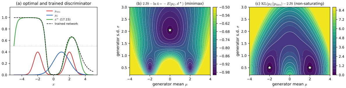
A flexible network trained on samples approaches \(d^\star\) closely: Figure 17.S1(a) overlays a 1-32-32-1 network trained by cross-entropy on 20 000 samples of each kind.
Definition 17.2 (Jensen–Shannon divergence) Exercise 17.1
For distributions \(P,Q\) with mixture \(M=\frac12(P+Q)\),
\[ \JS(P,Q)=\tfrac12\KL(P\|M)+\tfrac12\KL(Q\|M). \]This is the standard definition (Lin, 1991). The exercise calls the sum \(\KL(P\|M)+\KL(Q\|M)\) the Jensen–Shannon divergence, which is twice this; the factor matters only for the bound \(\JS\le\ln2\).
Result 17.2 (the generator objective is a Jensen–Shannon divergence) (17.16)–(17.17); Exercise 17.1
- At the optimal discriminator the error is \[ C(\pG)=E(\pG,d^\star)=-\int\pd\ln\frac{\pd}{\pd+\pG}\,\d\bx-\int\pG\ln\frac{\pG}{\pd+\pG}\,\d\bx, \tag{17.16} \] which equals \[ C(\pG)=\ln4-\KL\Big(\pd\,\Big\|\,\frac{\pd+\pG}2\Big)-\KL\Big(\pG\,\Big\|\,\frac{\pd+\pG}2\Big)=\ln4-2\JS(\pd,\pG). \] The book prints this as (17.17) with every sign reversed, \(-\ln4+\KL+\KL\), which is \(-C\) (Goodfellow's \(\max_DV\)); see the errata.
- \(0\le\JS\le\ln2\); \(\JS(P,Q)=\JS(Q,P)\); \(\JS=0\) if and only if \(P=Q\); \(\JS=\ln2\) if and only if \(P\) and \(Q\) have disjoint supports. Moreover \(\sqrt{\JS}\) is a metric (Endres and Schindelin, 2003).
- Hence the generator, which maximises the error, maximises \(C\), i.e. minimises \(\JS(\pd,\pG)\); the unique optimum is \(\pG=\pd\), where \(C=\ln4\), \(d^\star\equiv\frac12\), and the discriminator's error is that of guessing.
Proof
(1) Substituting (17.15) into (17.14) gives (17.16). Write \(\frac{p}{p+q}=\frac p{2M}\): then \(-\int p\ln\frac p{2M}\)
(2) Gibbs' inequality (Result 2.10; companion Result 1.22) gives \(\KL\ge0\) with equality iff the two arguments agree, so \(\JS\ge0\), with equality iff \(P=M=Q\). For the upper bound, \(\KL(P\|M)\)
(3) Follows from (1) and (2). ∎
Filling the gap 17.3: what Result 17.2 does not say pp. 536–537
"A fully optimised GAN matches the data" is true in function space with the discriminator optimised first. Three things separate it from practice.
Derivation
A weak equilibrium. \(E(q,d)\) is convex in \(d\) (pointwise, as in the proof of Result 17.1) and linear in \(q\). The pair \((q,d)=(p,\frac12)\) is a saddle point: \(E(p,d)\ge E(p,\frac12)=\ln4\) for every \(d\) (because \(\frac12=d^\star\) when \(q=p\)), and \(E(q,\frac12)\)
Parameters, not functions. Networks reach only some \(q\) and \(d\). If no generator equals \(\pd\), the best one depends on the divergence: in Figure 17.S1(b) the JS-optimal Gaussian sits between the two bumps. And in \((\bw,\bphi)\) the error is neither convex nor concave, so the saddle point need not attract gradient play.
Gradient play can circle. Near an equilibrium, gradient descent–ascent behaves like its linearisation, the vector field \(F(\bw,\bphi)\)
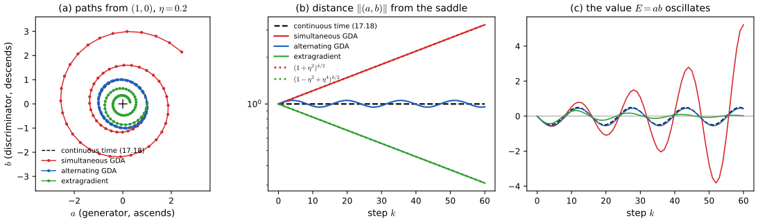
Result 17.3 (the bilinear game: flows circle, gradient steps diverge or cycle) Exercise 17.2, (17.18)–(17.20)
Let \(E(a,b)=ab\); \(a\) (the "generator") ascends and \(b\) (the "discriminator") descends, with step or rate \(\eta\).
- \((0,0)\) is the only stationary point; it is a saddle, with second derivative \(+2\) along \(b=a\) and \(-2\) along \(b=-a\).
- The gradient flow \(\dot a=\eta b\), \(\dot b=-\eta a\) started at \((1,0)\) is \(a=\cos\eta t\), \(b=-\sin\eta t\): the unit circle, forever.
- Simultaneous steps \((a,b)\leftarrow(a+\eta b,\,b-\eta a)\) multiply the distance to the saddle by \(\sqrt{1+\eta^2}\) each step: they spiral outwards.
- Alternating steps \(a\leftarrow a+\eta b\), then \(b\leftarrow b-\eta a\) (with the new \(a\)) preserve \(a^2+b^2+\eta ab\) exactly: for \(0<\eta<2\) they cycle on an ellipse and never converge.
- The extragradient method (Korpelevich, 1976), which takes a trial step and then steps with the gradient evaluated at the trial point, contracts the distance by \(\sqrt{1-\eta^2+\eta^4}<1\) per step (\(0<\eta<1\)) and converges.
Proof
(1) \(\nabla E=(b,a)\) vanishes only at the origin; the Hessian \(\begin{pmatrix}0&1\\1&0\end{pmatrix}\) has eigenvalues \(\pm1\) with eigenvectors along \(b=\pm a\); along \(b=a\), \(E=a^2\), with second derivative \(2\), and along \(b=-a\), \(E=-a^2\), with second derivative \(-2\).
(2) is Exercise 17.2, solved below.
(3)–(5) Write \(\bz=(a,b)^\T\) and \(J=\begin{pmatrix}0&1\\-1&0\end{pmatrix}\), so the update direction is \(J\bz\) and \(J^\T J=\bI\), \(J^\T=-J\), \(J^2=-\bI\). Simultaneous: \(\|(\bI+\eta J)\bz\|^2\)
Alternating updates are thus a real improvement over simultaneous ones (bounded instead of divergent), but neither converges; damping (momentum with a negative coefficient, extragradient, optimistic steps, or a regulariser such as the gradient penalty) is needed for convergence (Mescheder, Geiger and Nowozin, 2018).
Conditional GANs. p. 536 To sample from \(p(\bx\given\bc)\) (a chosen class, say), both networks receive \(\bc\) as an extra input and are trained on labelled pairs \((\bx_n,\bc_n)\) (Mirza and Osindero, 2014). One network for all classes shares its internal representations across them, which uses the data more efficiently than one GAN per class.
Result 17.4 (the conditional GAN optimum) p. 536
Let labels \(\bc\) have distribution \(p(\bc)\), data \(p(\bx\given\bc)\), and let the generator produce \(\pG(\bx\given\bc)\) for labels drawn from the same \(p(\bc)\). The optimal discriminator is \(d^\star(\bx,\bc)\)
maximised exactly when \(\pG(\cdot\given\bc)=p(\cdot\given\bc)\) for every \(\bc\) with \(p(\bc)>0\).
Proof
Apply Result 17.1 to the joint densities \(p(\bc)p(\bx\given\bc)\) and \(p(\bc)\pG(\bx\given\bc)\) of the pair \((\bx,\bc)\): the common factor \(p(\bc)\) cancels in \(d^\star\). In Result 17.2 the mixture is \(p(\bc)M(\bx\given\bc)\) with \(M=\frac12(p+\pG)\) conditionally, and \(\KL(p(\bc)p(\cdot\given\bc)\,\|\,p(\bc)M(\cdot\given\bc))\)
17.1.2 GAN training in practice
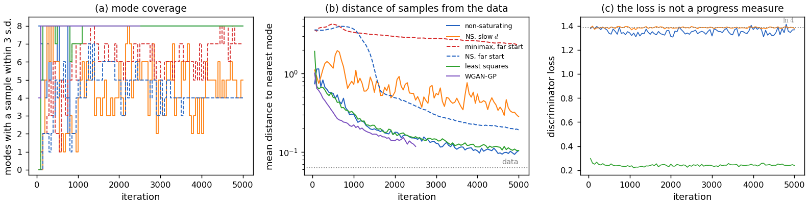
p. 536 GANs are hard to train because of the adversarial set-up, and the error can go up as well as down, so it does not measure progress (Exercise 17.2 and Figure 17.S5(c) below). One common failure is mode collapse: the generator maps all latent vectors to a small set of outputs, for instance only one digit. The book describes the discriminator as then assigning 1/2 to these outputs, after which training stops. That is not what the optimal discriminator does, and mode collapse is better understood as a best response.
Result 17.5 (mode collapse is the best response to a fixed discriminator) pp. 536–537
- For a fixed discriminator \(d\), both generator objectives, maximising \(-\E_q[\ln(1-d)]\) (minimax) and minimising \(\E_q[-\ln d]\) (non-saturating, (17.10)), are linear in \(q\), and their optimum over all distributions is attained by a point mass at any maximiser of \(d\) (when one exists).
- If instead the discriminator is optimal for the collapsed generator, it does not output 1/2 there: if \(q\) puts its mass on a region where \(\pd\) puts mass \(\pi\), then \(d^\star=\pi/(\pi+1)\) on that region in the sense of averages (about 1/9 for one mode out of eight), which pushes the generator away.
Proof and consequences
(1) \(\E_q[\ell]=\int q\ell\) with \(\ell=\ln(1-d)\) (to be minimised) or \(-\ln d\); both are decreasing functions of \(d\). For any \(q\), \(\int q\ell\ge\inf_\bx\ell(\bx)\), with equality for \(q=\delta_{\bx_0}\) at a minimiser of \(\ell\), i.e. a maximiser of \(d\). A generator that is improved against the current discriminator is therefore pulled towards concentrating its mass where \(d\) is largest. (2) By Result 17.1 applied to the sets \(A\) of the mode: \(\int_A\pd=\pi\), \(\int_A\pG=1\), and \(d^\star=\pd/(\pd+\pG)\) is small wherever \(\pG\) is large.
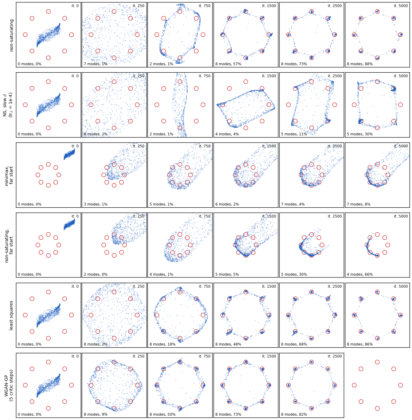
What actually happens. Real training sits between these two extremes: the discriminator takes a step or a few per generator step. The generator piles onto the modes the current \(d\) favours; the discriminator then lowers \(d\) there; the pile moves on. The result is mode hopping rather than a frozen state: in Figure 17.S5(a) the number of covered modes of the run with a slow discriminator swings between 2 and 8. Training "ceases" only if the discriminator cannot represent the difference, for example if it never sees enough samples at once to notice that a mode is missing (minibatch discrimination, Salimans et al., 2016, gives it that view). ∎
p. 537 Figure 17.2 shows why training can be slow. When data and generator distributions are far apart, the optimal discriminator is easy to learn and falls off very steeply, with almost zero gradient near both sets of samples. In the second term of (17.6), \(d(\bg(\bz,\bw),\bphi)\) is then essentially zero across the generated samples, so small changes of \(\bw\) barely change the error.
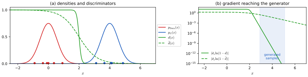
Filling the gap 17.4: Figure 17.2 in closed form p. 537
Derivation
For \(p=\N(m_0,s^2)\) and \(q=\N(m_1,s^2)\), \(d^\star=\sigma(a)\) with logit \(a(x)\)
p. 537 A smoothed discriminator \(\widetilde d\) gives the generator a stronger signal. The least-squares GAN (Mao et al., 2016) gets it with a real-valued discriminator trained by a sum-of-squares error; instance noise (Sønderby et al., 2016) adds Gaussian noise to both real and synthetic samples.
Filling the gap 17.5: vanishing gradients and instance noise p. 537
Why the gradient vanishes in general, why noise brings it back, and why noise does not change the answer.
Derivation
Vanishing. By Result 17.7(c), the minimax gradient against \(d^\star\) is \(\nabla_\btheta\,2\JS(\pd,\pG)\). When the two distributions do not overlap, JS is constant (\(\ln2\)) under any small change that keeps them apart (Result 17.8), so the gradient is exactly zero; when they overlap only in far tails it is exponentially small. For \(\pd=\N(0,0.3^2)\) and \(\pG=\N(4,0.3^2)\) the grid computation gives \(9\times10^{-10}\) (minimax) against 44 (non-saturating).
Noise. Replace every real and synthetic input \(\bx\) by \(\bx+\bm\epsilon\), \(\bm\epsilon\sim\N(\bzero,\tau^2\bI)\). The distributions become the convolutions \(p_\tau=p*\N_\tau\) and \(q_\tau=q*\N_\tau\), both positive everywhere and smooth; the optimal discriminator \(p_\tau/(p_\tau+q_\tau)\) is then smooth, and \(\JS(p_\tau,q_\tau)<\ln2\) responds to every movement of \(q\). For Gaussian mixtures convolution only adds \(\tau^2\) to each variance (confirmed numerically on the grid); with \(\tau=1\) the gradient in the example above becomes 0.15.
The optimum is unchanged. The characteristic function of \(\N(\bzero,\tau^2\bI)\), \(e^{-\tau^2\|\bm\omega\|^2/2}\), never vanishes, and convolution multiplies characteristic functions, so \(p_\tau=q_\tau\) implies \(p=q\). Minimising \(\JS(p_\tau,q_\tau)\) therefore still has \(\pG=\pd\) as its unique solution; in practice \(\tau\) is reduced during training. ∎
Result 17.6 (the least-squares GAN) p. 537; Mao et al. (2016)
Let the discriminator minimise \(\frac12\E_p[(d-b)^2]+\frac12\E_q[(d-a)^2]\) (target \(b\) for real, \(a\) for synthetic inputs) and the generator minimise \(\frac12\E_p[(d-c)^2]+\frac12\E_q[(d-c)^2]\) (the first term does not depend on the generator).
- The optimal discriminator is \(d^\star_{\rm LS}\)
\({}=\dfrac{bp+aq}{p+q}\) \({}=a+(b-a)\,\dfrac p{p+q}\), an affine function of the GAN optimum (17.15). - If \(b-c=1\) and \(b-a=2\) (e.g. \(a=-1\), \(b=1\), \(c=0\)), the generator's objective at \(d^\star_{\rm LS}\) is \(\frac12\int\frac{(p-q)^2}{p+q}\,\d\bx\)
\({}=\frac12\int\frac{(2q-(p+q))^2}{p+q}\,\d\bx\), half the Pearson \(\chi^2\) divergence of \(2q\) from \(p+q\); it is non-negative and vanishes only at \(q=p\).
Proof
(1) Pointwise, \(\frac12p(y-b)^2+\frac12q(y-a)^2\) is a convex quadratic in \(y=d(\bx)\) with minimum where \(p(y-b)+q(y-a)=0\). (2) \(d^\star_{\rm LS}-c\)
Part (1) shows that, at the optimum, the least-squares discriminator is exactly as steep as the GAN one: the smoothing of Figure 17.2 cannot come from the optimum. It comes from what a discriminator of limited capacity does during training (next box), and from the loss \((d-c)^2\), whose gradient does not vanish when \(d\) is far from \(c\).
Filling the gap 17.6: why least squares smooths a finite discriminator p. 537
Derivation
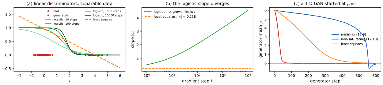
Take the simplest discriminator, linear in \(x\), and real and synthetic samples that a threshold separates. Cross-entropy, \[ -\sum_n\big[t_n\ln\sigma(wx_n+b)+(1-t_n)\ln(1-\sigma(wx_n+b))\big], \] has no minimiser: scaling a separating \((w,b)\) by \(k>1\) lowers every term, so gradient descent drives \(|w|\to\infty\), the sigmoid becomes a step, and its gradient vanishes at the samples. On separable data the norm grows only logarithmically in the number of steps while the direction converges to the maximum-margin separator (Soudry et al., 2018); Figure 17.S6(b) shows \(|w|\) gaining the same amount per decade of steps. Least squares has the unique minimiser given by the normal equations (a finite slope, 0.238 here), and the generator's loss \((wx+b-1)^2\) has gradient \(2(wx+b-1)w\), which does not decay when the samples are rejected. Panel (c) runs a one-dimensional GAN (data \(\N(0,1)\), generator \(x=\mu+z\) started at \(\mu=6\), five discriminator steps per generator step): after 300 generator steps the minimax generator has moved to 5.18, the least-squares one to 1.00, and the non-saturating one has arrived (\(-0.02\)). ∎
pp. 537–538 The most common change (Mescheder, Geiger and Nowozin, 2018, review many others) replaces the generator's term
\[ -\frac1{N_{\rm synth}}\sum_{n\in\rm synth}\ln\big(1-d(\bg(\bz_n,\bw),\bphi)\big) \tag{17.9} \]by
\[ \frac1{N_{\rm synth}}\sum_{n\in\rm synth}\ln d(\bg(\bz_n,\bw),\bphi), \tag{17.10} \]still to be maximised by the generator: instead of making a sample less likely to be called fake, it makes it more likely to be called real. Figure 17.3 compares the two.
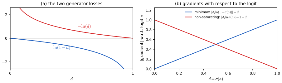
Result 17.7 (the non-saturating loss) p. 538, (17.9)–(17.10), Figure 17.3
- With \(d=\sigma(a)\): \(\partial_a\ln(1-\sigma(a))\)
\({}=-\sigma(a)\) \({}=-d\) and \(\partial_a\big(-\ln\sigma(a)\big)\) \({}=-(1-\sigma(a))\) \({}=-(1-d)\). - Both generator losses have the same fixed point in function space: at \(\pG=\pd\) the optimal discriminator is constant, so neither loss changes to first order under any perturbation of \(\pG\) that keeps its total mass.
- Let \(q_\btheta\) be a family of generator densities and freeze the optimal discriminator \(d^\star_0\) of \(q_{\btheta_0}\). At \(\btheta=\btheta_0\), \[ \nabla_\btheta\E_{q_\btheta}\big[\ln(1-d^\star_0)\big]=\nabla_\btheta\,2\JS(\pd,q_\btheta),\qquad \nabla_\btheta\E_{q_\btheta}\big[-\ln d^\star_0\big]=\nabla_\btheta\big[\KL(q_\btheta\|\pd)-2\JS(\pd,q_\btheta)\big]. \] So the minimax generator descends JS, while the non-saturating one descends a reverse KL minus twice JS (Arjovsky and Bottou, 2017).
Proof
(1) \(\sigma'=\sigma(1-\sigma)\), so \(\partial_a\ln(1-\sigma)\)
(2) At \(q=p\), \(d^\star=\frac12\), so both \(\E_q[\ln(1-d^\star)]\) and \(\E_q[-\ln d^\star]\) are \(\int q\cdot\ln\frac12\) and \(\int\delta q\cdot\ln\frac12=0\) for any perturbation with \(\int\delta q=0\).
(3) Write \(q=q_\btheta\), \(\dot q=\partial q/\partial\theta_i\), and assume differentiation under the integral is allowed. From (17.16) and Result 17.2, \(2\JS(p,q)-\ln4\)
Consequence: mode dropping. \(\KL(q\|p)\) is huge where \(q\) puts mass and \(p\) has none, but costs little when \(q\) ignores part of \(p\) (the mode-seeking property of the reverse KL; companion Section 10.1.2). On two bumps the non-saturating objective is minimised by a Gaussian on one bump (Figure 17.S1(c)), and descent against \(d^\star\) ends there: \((\mu,\sigma)=(2,0.5)\), while the minimax descent ends at the covering Gaussian \((0,2.04)\). The non-saturating loss buys strong gradients at the price of this bias, which is consistent with the far-start ring run of Figure 17.S4 arriving fast but collapsing onto four modes.
Wasserstein GANs
p. 538 A more direct remedy is to measure how far apart \(\pG\) and \(\pd\) are in data space. The Wasserstein or earth mover's distance pictures \(\pG\) as a pile of earth to be reshaped into \(\pd\): it is the least possible amount of earth times average distance moved. It cannot be computed directly; the Wasserstein GAN (Arjovsky, Chintala and Bottou, 2017) approximates it with a real-valued discriminator (a critic) whose input gradient \(\nabla_\bx d(\bx,\bphi)\) is kept bounded by weight clipping, and the gradient-penalty version (Gulrajani et al., 2017) replaces the clipping by a penalty. First, why JS is the wrong yardstick when supports do not overlap.
Result 17.8 (JS cannot see distances between disjoint distributions) pp. 537–538
If \(P\) and \(Q\) are concentrated on disjoint sets \(A\) and \(B\), then \(\JS(P,Q)=\ln2\), \(\KL(P\|Q)=\KL(Q\|P)=\infty\), the indicator of \(A\) is an optimal discriminator with error 0, and for any family \(Q_\btheta\) that stays disjoint from \(A\) near \(\btheta_0\), \(\nabla_\btheta\JS(P,Q_\btheta)=\bzero\) there. When \(\pG\) is supported on the image of a lower-dimensional latent space (Filling the gap 17.1) and \(\pd\) is concentrated near a low-dimensional data manifold, the two supports generically do not overlap, so this is the typical situation early in training (Arjovsky and Bottou, 2017).
Proof
On \(A\), \(q=0\) and \(M=p/2\), so \(\KL(P\|M)=\int_Ap\ln2=\ln2\); likewise \(\KL(Q\|M)=\ln2\); hence \(\JS=\ln2\) whatever the distance between \(A\) and \(B\). \(\KL(P\|Q)=\int p\ln(p/q)\) has \(q=0\) where \(p>0\). The indicator of \(A\) gives \(-\ln1\) on real and \(-\ln(1-0)\) on synthetic samples, i.e. zero error. A constant function of \(\btheta\) has zero gradient. ∎ For \(P=U[0,1]\) and \(Q=U[\theta,\theta+1]\): \(\JS=|\theta|\ln2\) for \(|\theta|\le1\) and \(\ln2\) beyond, while the earth mover's distance is \(|\theta|\) (Figure 17.S7(a)).
Definition 17.3 (Wasserstein-1 distance) p. 538
For distributions \(P,Q\) on \(\R^D\) with finite means, a coupling is a joint distribution \(\gamma\) of \((\bx,\by)\) with marginals \(P\) and \(Q\) (a transport plan: \(\gamma(\bx,\by)\) is the amount of earth moved from \(\by\) to \(\bx\)). The Wasserstein-1 distance is the cheapest plan's average distance,
\[ \W(P,Q)=\inf_{\gamma\in\Pi(P,Q)}\E_{(\bx,\by)\sim\gamma}\|\bx-\by\| . \]Result 17.9 (one dimension, and the Kantorovich–Rubinstein duality) p. 538
For distributions on \(\R\) with distribution functions \(F_P,F_Q\) and quantile functions \(F_P^{-1},F_Q^{-1}\),
\[ \W(P,Q)=\int_{-\infty}^{\infty}|F_P(x)-F_Q(x)|\,\d x=\int_0^1|F_P^{-1}(u)-F_Q^{-1}(u)|\,\d u=\sup_{\Lip(f)\le1}\big(\E_P[f]-\E_Q[f]\big), \]the infimum is attained by the quantile coupling \((F_P^{-1}(U),F_Q^{-1}(U))\), \(U\sim U(0,1)\), and the supremum by the optimal critic \(f^\star\) with \(f^{\star\prime}=\sgn(F_Q-F_P)\). In any dimension, the equality of the infimum and the supremum over 1-Lipschitz functions (Kantorovich–Rubinstein duality) still holds (Villani, 2009, Chapter 5); the WGAN critic is a network that approximates the supremum.
Proof (complete in one dimension)
Weak duality (any dimension). For a coupling \(\gamma\) and \(\Lip(f)\le1\), \(\E_P f-\E_Q f\)
The supremum equals the area between the distribution functions. A 1-Lipschitz \(f\) is absolutely continuous with \(|f'|\le1\). Integrating by parts (for finite means the boundary terms vanish), \[ \E_P f=f(0)+\int_0^\infty f'(x)(1-F_P(x))\,\d x-\int_{-\infty}^0f'(x)F_P(x)\,\d x ; \] subtracting the same expression for \(Q\),
\[ \E_P f-\E_Q f=\int_{-\infty}^\infty f'(x)\big(F_Q(x)-F_P(x)\big)\,\d x\le\int|F_Q-F_P|\,\d x , \]with equality for \(f'=\sgn(F_Q-F_P)\).
The quantile coupling costs the same area. Its cost \(\int_0^1|F_P^{-1}(u)-F_Q^{-1}(u)|\,\d u\) is the area of the region between the graphs of \(F_P\) and \(F_Q\) measured in horizontal strips, and \(\int|F_P-F_Q|\,\d x\) is the same area measured in vertical strips (Fubini). So \(\inf\le\int|F_P-F_Q|=\sup\le\inf\), and all are equal. ∎
Numerically: for ten random pairs of mixtures the two integrals agree to \(2\times10^{-3}\) on the grid and match the optimal transport of \(2\times10^5\) sorted samples; \(\E_Pf^\star-\E_Qf^\star=\W\) to \(10^{-6}\), and 200 random 1-Lipschitz functions all give less. For a translation, \(F_Q^{-1}(u)=F_P^{-1}(u)+\theta\), so \(\W=|\theta|\).
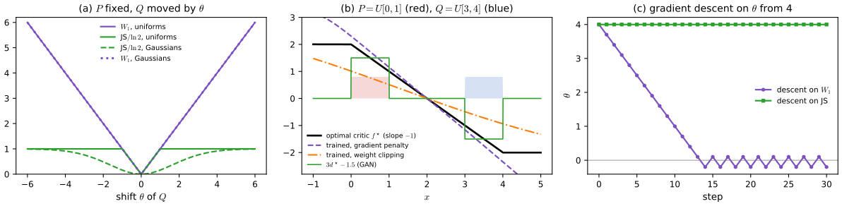
Result 17.10 (the Wasserstein loss is continuous in the generator's parameters) p. 538; Arjovsky, Chintala and Bottou (2017)
If \(\|\bg(\bz,\btheta)-\bg(\bz,\btheta')\|\)
Proof
\(\W\) is a metric (it is symmetric, vanishes only for equal distributions, and obeys the triangle inequality by gluing an optimal plan from \(P\) to \(Q\) with one from \(Q\) to \(R\); Villani, 2009, Chapter 6). Hence \(|\W(\pd,P_\btheta)-\W(\pd,P_{\btheta'})|\)
p. 538 The gradient-penalty WGAN is written in the book as
\[ E_{\rm WGAN\text{-}GP}(\bw,\bphi)=-\frac1{N_{\rm real}}\sum_{n\in\rm real}\Big[\ln d(\bx_n,\bphi)-\eta\big(\|\nabla_{\bx_n}d(\bx_n,\bphi)\|^2-1\big)^2\Big]+\frac1{N_{\rm synth}}\sum_{n\in\rm synth}\ln d(\bg(\bz_n,\bw,\bphi)) \tag{17.11} \]where \(\eta\) weights the penalty. This differs from the method it cites in four ways (see the next box and the errata); the version that Gulrajani et al. (2017) actually use, and that the demo and code implement, is
\[ E_{\rm critic}(\bphi)=\frac1{N}\sum_{n}d(\bg(\bz_n,\bw),\bphi)-\frac1N\sum_nd(\bx_n,\bphi)+\frac\eta N\sum_n\big(\|\nabla_\bx d(\widehat\bx_n,\bphi)\|-1\big)^2,\qquad \widehat\bx_n=\epsilon_n\bx_n+(1-\epsilon_n)\bg(\bz_n,\bw), \]with \(\epsilon_n\sim U(0,1)\), minimised over \(\bphi\), while the generator minimises \(-\frac1N\sum_nd(\bg(\bz_n,\bw),\bphi)\).
Filling the gap 17.7: the Lipschitz constraint, weight clipping and the gradient penalty p. 538
Derivation
Lipschitz means bounded gradient. For differentiable \(f\), \(\Lip(f)\le1\) if and only if \(\|\nabla f(\bx)\|\le1\) everywhere: by the mean value theorem \(|f(\bx)-f(\by)|\)
Weight clipping keeps every weight in \([-c,c]\). For a network with 1-Lipschitz activations, \(\Lip(f)\)
Why penalise at interpolates. Result 17.11 shows that an optimal critic has gradient norm exactly 1 on the segments between points that the optimal plan couples. Real and generated samples paired at random are a cheap stand-in for coupled pairs, and points \(\widehat\bx\) on the segments between them are where the constraint is active. Penalising at the real points only, as (17.11) is written, constrains the critic where its gradient matters least.
The penalty is a soft constraint. For \(P=U[0,1]\), \(Q=U[3,4]\) and linear critics \(f(x)=sx\), the objective \(\E_Pf-\E_Qf-\lambda(|s|-1)^2\)
Result 17.11 (the optimal critic has unit slope along transport paths) Gulrajani et al. (2017), Proposition 1
Let \(f^\star\) attain the supremum in Result 17.9 and \(\gamma^\star\) the infimum. Then \(f^\star(\bx)-f^\star(\by)=\|\bx-\by\|\) for \(\gamma^\star\)-almost every pair, \(f^\star\) is linear with slope 1 on the segment from \(\by\) to \(\bx\), and wherever \(f^\star\) is differentiable on that segment, \(\nabla f^\star=(\bx-\by)/\|\bx-\by\|\).
Proof
By duality, \(\E_{\gamma^\star}[f^\star(\bx)-f^\star(\by)]\)
17.2 Image GANs
See also this course, Section 10.5.2 (up-sampling and transposed convolutions, Result 10.9) and the convolution arithmetic demo.
p. 539 Images are the most successful application of GANs. Early GANs used fully connected networks, but convolutional ones work much better: the discriminator is an ordinary convolutional classifier, and the generator maps a low-dimensional \(\bz\) to a large image through transposed convolutions (the book's Figure 17.4, a DCGAN diagram from \(\bz\in\R^{100}\) through \(4\times4\times1024\), \(8\times8\times512\), \(16\times16\times256\) and \(32\times32\times128\) to a \(64\times64\times3\) image). Progressive growing of both networks, from \(4\times4\) up to \(1024\times1024\) images, speeds up training and allows very high resolution (Karras et al., 2017); BigGAN (Brock, Donahue and Simonyan, 2018; the book's Figure 17.5) is a class-conditional generator with residual blocks and about 70 million parameters. Neither diagram is reproduced.
Filling the gap 17.8: the sizes in Figure 17.4 p. 539, Figure 17.4
Derivation
A transposed convolution with kernel \(k\), stride \(s\) and padding \(p\) maps width \(i\) to \(o=s(i-1)+k-2p\) (it is the adjoint of the strided convolution mapping \(o\) to \(i\); Result 10.9). With \(k=4\), \(s=2\), \(p=1\), \(o=2i\), giving \(4\to8\to16\to32\to64\). PyTorch confirms the sizes and the adjoint identity \(\langle\mathrm{conv}(\bx),\by\rangle\)
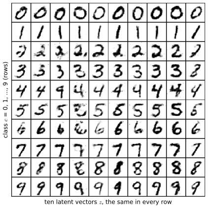
p. 542 GANs also learn representations (Section 6.3.3). A DCGAN trained on bedroom images (Radford, Metz and Chintala, 2015) produces bedrooms, and its latent space is organised: a smooth path in \(\bz\) gives a smooth sequence of plausible images (the book's Figure 17.9), and some directions correspond to meaningful changes such as pose, lighting or a smile, disentangled representations that support arithmetic on latent vectors (Figure 17.10). Below, both phenomena are reproduced with a small GAN on MNIST.
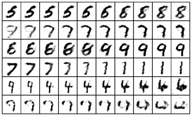
Filling the gap 17.9: how to walk in a Gaussian latent space, and why three vectors per group pp. 542–543
Derivation
Norms concentrate. For \(\bz\sim\N(\bzero,\bI_D)\), \(\|\bz\|^2\) is \(\chi^2_D\), with mean \(D\) and variance \(2D\), so \(\|\bz\|/\sqrt D\to1\): in \(D=32\) almost all latent vectors lie near the sphere of radius \(\sqrt{32}\approx5.7\), and the generator has been trained only there. The midpoint of a straight line between two independent latents, \((\bz_1+\bz_2)/2\sim\N(\bzero,\frac12\bI)\), has \(\E\|\cdot\|^2=D/2\): it lies well inside the sphere, in a region the generator never saw (a simulation gives \(0.500D\)). Spherical interpolation \(\mathrm{slerp}(\bz_1,\bz_2;t)\)
Averaging and arithmetic. The mean of \(k\) independent latents has covariance \(\bI/k\), so it is shorter than a typical latent by \(\sqrt k\). The arithmetic of Figure 17.10, \(\bar\bz_A-\bar\bz_B+\bar\bz_C\) with three vectors per group, has covariance \(3\cdot\bI/3=\bI\) if the nine vectors are independent: the result is again a typical latent vector, while the averages remove much of the individual variation. ∎
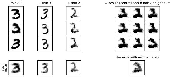
Why does pixel arithmetic fail where latent arithmetic works? An average of images is an image only if the images are aligned; strokes at slightly different places superpose as ghosts (the bottom right of Figure 17.10, and the bottom row of the book's Figure 17.10). The generator maps latent vectors back onto (an approximation of) the set of digit images, so arithmetic done before the generator ends on that set.
17.2.1 CycleGAN
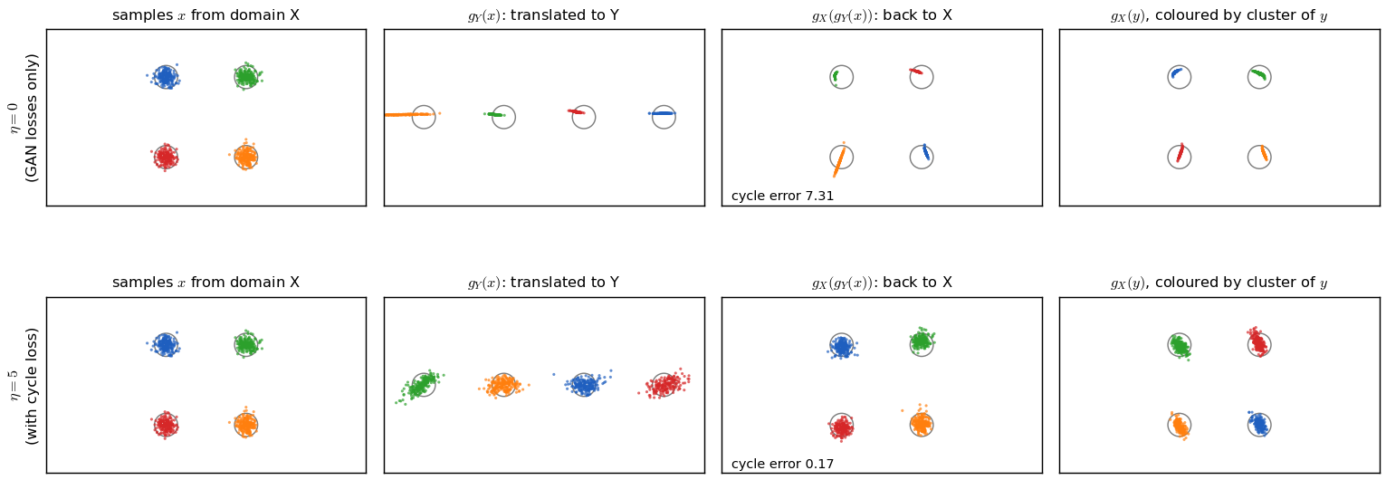
pp. 539–542 CycleGAN (Zhu et al., 2017) learns to translate between two domains, for example photographs \(X\) and Monet paintings \(Y\), from two unpaired collections (the book's Figure 17.6 shows translations in both directions). It has two conditional generators, \(\bg_X(\by,\bw_X)\) turning a painting into a photograph and \(\bg_Y(\bx,\bw_Y)\) turning a photograph into a painting, and two discriminators \(d_X\) (real or synthetic photograph?) and \(d_Y\) (real or synthetic painting?). The usual GAN errors alone would make the outputs look like the right domain, but nothing would tie a painting to the photograph it came from. CycleGAN adds the cycle-consistency error (the book's Figure 17.7): a photograph translated to a painting and back should return to itself, and likewise for paintings,
\[ E_{\rm cyc}(\bw_X,\bw_Y)=\frac1{N_X}\sum_{n\in X}\|\bg_X(\bg_Y(\bx_n))-\bx_n\|_1+\frac1{N_Y}\sum_{n\in Y}\|\bg_Y(\bg_X(\by_n))-\by_n\|_1 , \tag{17.12} \]with \(\|\cdot\|_1\) the L1 norm, and the total error (whose information flow is the book's Figure 17.8, a diagram not reproduced) is
\[ E_{\rm GAN}(\bw_X,\bphi_X)+E_{\rm GAN}(\bw_Y,\bphi_Y)+\eta E_{\rm cyc}(\bw_X,\bw_Y) . \tag{17.13} \]Result 17.12 (what cycle consistency does and does not determine) pp. 540–542, (17.12)–(17.13)
- The GAN errors alone constrain only the distributions: if \(\bg_Y\) maps \(p_X\) to \(p_Y\), so does \(T\circ\bg_Y\) for any map \(T\) that leaves \(p_Y\) unchanged (a permutation of clusters, a symmetry of the domain), and \(\bg_Y\) may also discard information (map many photographs to one painting).
- If \(E_{\rm cyc}=0\) (in the population limit), then \(\bg_X(\bg_Y(\bx))=\bx\) for \(p_X\)-almost every \(\bx\): \(\bg_Y\) is injective on the support of \(p_X\) and \(\bg_X\) inverts it there. With both terms zero and both GAN errors at their optimum, \(\bg_Y\) is a bijection between the supports (up to null sets) with inverse \(\bg_X\).
- Cycle consistency still allows every bijection compatible with the distributions; which one is learned depends on the networks' inductive biases. The L1 norm makes the error robust to outliers: its pointwise minimiser is a median, not a mean (companion Result 1.19).
Proof
(1) The GAN error of \(\bg_Y\) depends on \(\bg_Y\) only through the distribution of \(\bg_Y(\bx)\), which is unchanged by \(T\). (2) A non-negative integrand with zero integral vanishes almost everywhere; \(\bg_X\circ\bg_Y=\mathrm{id}\) on a set implies \(\bg_Y\) is injective there (equal images would give equal pre-images). If also \(\bg_Y\circ\bg_X=\mathrm{id}\) on the support of \(p_Y\), each map is onto the other's support up to null sets, so they are mutually inverse bijections. (3) Any bijection \(\bg_Y\) pushing \(p_X\) to \(p_Y\), with \(\bg_X=\bg_Y^{-1}\), makes all three errors optimal. ∎
Beyond the book: evaluating generative models
The book does not discuss how to tell whether a GAN is good, but the question is unavoidable: its loss is no guide (Figure 17.S5(c)) and it has no likelihood (Filling the gap 17.1). Practice compares statistics of generated and real samples in the feature space of a pretrained classifier. Below the classifier is a small MNIST network (95.0% test accuracy) and its 256 hidden units are the features.
Filling the gap 17.10: the inception score is a mutual information supplement
Derivation
With a classifier \(p(y\given\bx)\) over \(K\) classes and \(p(y)=\E_{\bx\sim\pG}p(y\given\bx)\), the inception score (Salimans et al., 2016) is \(\mathrm{IS}\)
Result 17.13 (the Fréchet distance is a Wasserstein distance between Gaussians) supplement; Heusel et al. (2017)
Fit Gaussians \(\N(\bmu_1,\Sig_1)\) and \(\N(\bmu_2,\Sig_2)\) to the features of real and generated images. Then
\[ \mathrm{FD}=\|\bmu_1-\bmu_2\|^2+\Tr\Big(\Sig_1+\Sig_2-2\big(\Sig_1^{1/2}\Sig_2\Sig_1^{1/2}\big)^{1/2}\Big) \]is the squared Wasserstein-2 distance \(\inf_\gamma\E_\gamma\|\bx-\by\|^2\) between the two Gaussians (Dowson and Landau, 1982); computed in the features of an Inception network it is the FID.
Proof (the transport map; optimality cited)
Centre both (the means contribute \(\|\bmu_1-\bmu_2\|^2\) to any coupling's cost, since the cross term has mean zero). Let \(T\)
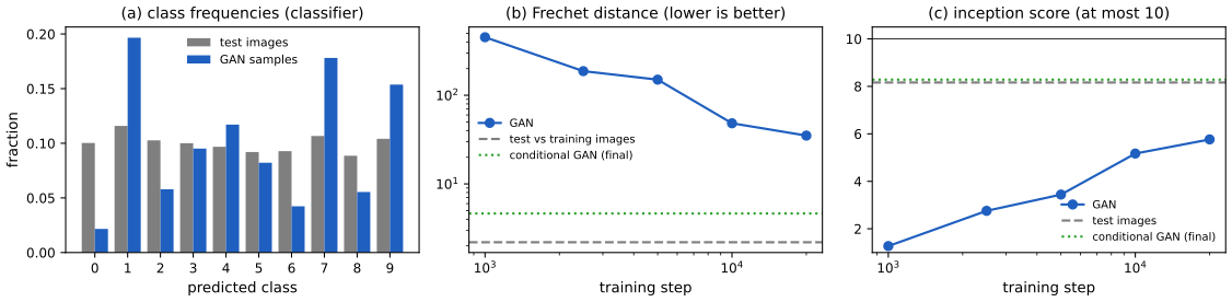
On the ring the same questions have exact answers: the number of modes with nearby samples measures diversity (recall) and the fraction of samples near a mode measures quality (precision), which is how Figures 17.S4–17.S5 and the ring demo report progress.
Summary: errors and imprecisions found in the chapter (first printing)
- (17.17) and Exercise 17.1: the printed (17.17), \(-\ln4+\KL(p\|M)+\KL(q\|M)\), is the negative of (17.16). Each integrand of (17.16) is non-negative, so (17.16) \(\ge0\), while the printed (17.17) \(\le0\); the correct identity is (17.16) \(=\ln4-\KL(p\|M)-\KL(q\|M)\) (for the densities of Figure 17.S1(a): 0.7670 against \(-0.7670\); Result 17.2). Accordingly, the "minimum of \(C(\pG)\)" at \(\pG=\pd\) is a minimum of the printed expression (Goodfellow et al.'s \(C(G)=\max_DV\)) but a maximum of the error (17.16), as it must be for a generator that maximises \(E\) (17.8).
- Exercise 17.1: the sum \(\KL(p\|M)+\KL(q\|M)\) is twice the Jensen–Shannon divergence as usually defined (Lin, 1991), which is bounded by \(\ln2\); the sum is bounded by \(2\ln2\).
- (17.11) does not match Gulrajani et al. (2017): (i) a Wasserstein critic is real-valued and enters linearly; \(\ln d\) is undefined for \(d\le0\) (and would make the error a different divergence); (ii) the penalty is \((\|\nabla_\bx d\|-1)^2\), not \((\|\nabla_\bx d\|^2-1)^2\); (iii) it is evaluated at random points \(\widehat\bx_n\) between real and generated samples, not at the real points; (iv) \(\bg(\bz_n,\bw,\bphi)\) should be \(\bg(\bz_n,\bw)\). The corrected form is given after Result 17.10.
- p. 536 (imprecision): in mode collapse the discriminator does not settle at 0.5 on the collapsed outputs; the optimal one is well below 1/2 there (about 1/9 for one of eight equal modes), and training typically hops between modes rather than ceasing (Result 17.5, Figure 17.S5(a)).
- p. 538 (imprecision): when \(d(\bg(\bz,\bw))\approx0\), "the first form has a very small gradient" holds with respect to the discriminator's logit (a factor \(d\)), not with respect to \(d\), where the slope of \(\ln(1-d)\) is \(-1\) (Result 17.7(1)). In Figure 17.3 the horizontal axis is labelled \(x\) but is \(d\).
- Typography: p. 534 "along with with"; p. 537 "one§-dimensional" (stray symbol).
Exercises
All three exercises of Chapter 17 (Bishop and Bishop, 2024, pp. 544–545), restated in my own words, with complete solutions (hidden). Stars give the book's difficulty. The official solutions manual stops at Chapter 10, so these solutions are my own.
Exercise 17.1 (★★★). Prove that, with unlimited flexibility, the GAN's solution is the data distribution. Optimise over all distributions \(\pG\) and all functions \(d\), with \(d\) optimised in an inner loop. (a) Show that in the limit of infinitely many samples (17.6) becomes (17.14). (b) Show by a variational argument that the optimal \(d\) for fixed \(\pG\) is (17.15). (c) Show that the error then becomes (17.16), (d) rewrite it with Kullback–Leibler divergences as in (17.17), and (e) use \(\KL\ge0\), with equality only for equal arguments, to show that the optimum is \(\pG=\pd\). The two KL terms together form the Jensen–Shannon divergence, which, unlike KL, is symmetric.
Solution
(a) The real \(\bx_n\) are independent draws from \(\pd\), and the \(\bg(\bz_n,\bw)\), \(\bz_n\sim p(\bz)\), independent draws from \(\pG\). By the strong law of large numbers, \(\frac1{N_{\rm real}}\sum\ln d(\bx_n)\)
\({}\to\int\pd\ln d\) and \(\frac1{N_{\rm synth}}\sum\ln(1-d(\bg(\bz_n,\bw)))\) \({}\to\int\pG\ln(1-d)\) almost surely (whenever these integrals are finite), which is (17.14) (Filling the gap 17.2). (b) Perturb \(d\) to \(d+\epsilon\eta\) for an arbitrary function \(\eta\): \(\frac{\d}{\d\epsilon}E\big|_{\epsilon=0}\)
\({}=\int\big(-\frac{\pd}{d}+\frac{\pG}{1-d}\big)\eta\,\d\bx\). This vanishes for every \(\eta\) iff the bracket is zero, i.e. \(\pd(1-d)=\pG d\), i.e. (17.15). The second variation \(\int\big(\frac{\pd}{d^2}+\frac{\pG}{(1-d)^2}\big)\eta^2\) \({}\ge0\), so this is a minimum; Result 17.1 shows it is the global minimum. (c) Substituting \(d^\star\) and \(1-d^\star=\pG/(\pd+\pG)\) into (17.14) gives (17.16).
(d) With \(M=(\pd+\pG)/2\), \(\frac{\pd}{\pd+\pG}=\frac{\pd}{2M}\), so \(-\int\pd\ln\frac{\pd}{2M}\)
\({}=\ln2-\KL(\pd\|M)\), and likewise for \(\pG\): (17.16) \(=\ln4-\KL(\pd\|M)-\KL(\pG\|M)\). This is (17.17) with all signs reversed; the printed (17.17) is \(-C\) (errata). (e) Both KL terms are \(\ge0\) and vanish iff \(\pd=M\) and \(\pG=M\), i.e. iff \(\pG=\pd\). So \(C(\pG)\le\ln4\) with equality iff \(\pG=\pd\): the generator, which maximises the error, attains its best value \(\ln4\) exactly at the data distribution, where \(d^\star\equiv\frac12\). In the printed form, \(-\ln4+\KL+\KL\ge-\ln4\) with the same equality case, which is the "minimum" of the exercise. The sum \(\KL(\pd\|M)+\KL(\pG\|M)\) is \(2\JS\) in the usual normalisation (Definition 17.2); it is symmetric because swapping \(\pd\) and \(\pG\) leaves \(M\) unchanged and swaps the two terms. Numerical confirmation: Result 17.2 and the demo, preset 2.
Exercise 17.2 (★★★). Let \(E(a,b)=ab\), with \(a\) playing the generator and \(b\) the discriminator. Show that \((0,0)\) is a stationary point, and, from the second derivatives along \(b=a\) and \(b=-a\), that it is a saddle. In continuous time, with \(a\) ascending and \(b\) descending, the parameters follow (17.18), \(\dot a=\eta\,\partial E/\partial a\), \(\dot b=-\eta\,\partial E/\partial b\). Show that \(a\) satisfies \(\ddot a=-\eta^2a\) (17.19), that \(a=C\cos\eta t+D\sin\eta t\) (17.20) solves it, find \(C,D\) for the start \(a=1\), \(b=0\), and show that \((a,b)\) then moves on the unit circle and never reaches the saddle.
Solution
Stationary point and saddle. \(\partial E/\partial a=b\) and \(\partial E/\partial b=a\) both vanish at the origin. Along \(b=a\), \(E=a^2\), whose second derivative in \(a\) is \(+2\) (a minimum along this line); along \(b=-a\), \(E=-a^2\), second derivative \(-2\) (a maximum). A point that is a minimum along one line and a maximum along another is a saddle; equivalently the Hessian \(\begin{pmatrix}0&1\\1&0\end{pmatrix}\) has eigenvalues \(\pm1\).
Dynamics. (17.18) reads \(\dot a=\eta b\), \(\dot b=-\eta a\). Differentiating the first and substituting the second, \(\ddot a=\eta\dot b=-\eta^2a\), which is (17.19). For (17.20), \(\dot a=\eta(-C\sin\eta t+D\cos\eta t)\) and \(\ddot a\)
\({}=-\eta^2(C\cos\eta t+D\sin\eta t)\) \({}=-\eta^2a\). Initial conditions: \(a(0)=C=1\), and \(\dot a(0)=\eta D=\eta b(0)=0\), so \(D=0\). Hence \(a=\cos\eta t\) and \(b=\dot a/\eta=-\sin\eta t\), so \(a^2+b^2=1\) for all \(t\): the point moves clockwise round the unit circle with period \(2\pi/\eta\) and its distance from the saddle never changes. (Directly: \(\frac{\d}{\d t}(a^2+b^2)\) \({}=2a\eta b-2b\eta a\) \({}=0\).) Discrete steps do worse or the same: simultaneous gradient steps spiral outwards, alternating steps cycle, and only a corrected method such as extragradient converges (Result 17.3, Figure 17.S2). Integrating (17.18) numerically matches \(\cos\eta t\), \(-\sin\eta t\) to \(10^{-11}\).
Exercise 17.3 (★). The training set contains equal numbers of cat and dog images, and the generator has learned to produce high-quality dog images. Show that the optimal discriminator outputs \(1/3\) on a dog image.
Solution
Write \(\pd\)
\[ d^\star=\frac{\frac12p_{\rm dog}}{\frac12p_{\rm dog}+p_{\rm dog}}=\frac13 , \]\({}=\frac12p_{\rm cat}+\frac12p_{\rm dog}\) and, reading "high-quality dog images" as "distributed like the dogs in the data", \(\pG=p_{\rm dog}\). Assume cat and dog images do not overlap, so \(p_{\rm cat}=0\) on dog images. By (17.15), on a dog image and on a cat image \(d^\star=1\). Interpretation: a dog image comes from the data with prior 1/2, but the data produce dogs at half the generator's rate, so the posterior odds of "real" are \(\frac12:1\). The generator is not at the optimum: \(\JS\)
\({}=\frac12\KL(\pd\|M)+\frac12\KL(\pG\|M)\) with \(M\) \({}=\frac14p_{\rm cat}+\frac34p_{\rm dog}\) gives \(\JS\) \({}=\frac12\big[\frac12\ln2+\frac12\ln\frac23\big]+\frac12\ln\frac43\) \({}=\frac34\ln\frac43\) \({}\approx0.216\), and the error (17.16) is \(\ln4-2\JS\approx0.955<\ln4\), so the generator can still gain by producing cats. If cats and dogs did overlap, the answer would be \(\frac{p_{\rm cat}+p_{\rm dog}}{p_{\rm cat}+3p_{\rm dog}}\), equal to \(1/3\) only where \(p_{\rm cat}=0\). The demo, preset 3, shows \(d^\star=1/3\) on the "dog" bump and 1 on the "cat" bump.
Demonstrations
Three interactive pages, each linked above where its topic arises. They run in the browser and reproduce the Python code number for number (largest differences between page and Python \(8\times10^{-14}\) for 200 iterations of the ring GAN with each loss, \(10^{-13}\) for the optimal-discriminator quantities and descent paths, \(10^{-12}\) for the Wasserstein and JS curves). The companion course has no GAN demonstration; its VAE latent explorer, normalizing-flow and diffusion demos show the likelihood-based alternatives.
- Training a GAN on a ring of Gaussians: generator and discriminator trained live with hand-written backpropagation (including the double backpropagation of the gradient penalty); five losses, two learning rates, discriminator steps, a far start. Presets: 1 non-saturating, 2 mode collapse, 3 far start, minimax, 4 far start, non-saturating, 5 WGAN-GP.
- The optimal discriminator and the Jensen–Shannon divergence: \(d^\star\), JS, KL and \(\W\) for a Gaussian generator against four data densities, instance noise, and gradient descent against \(d^\star\) with each loss. Presets: 1 the optimal discriminator, 2 \(\pG=\pd\), 3 Exercise 17.3, 4 vanishing gradient, 5 non-saturating descent.
- Wasserstein versus Jensen–Shannon: move one distribution away from another; the transport plan, the area between distribution functions, the optimal critic and the GAN discriminator, and descent on either distance. Presets: 1 disjoint uniforms, 2 descent on each, 3 Gaussians, 4 narrow peaks, 5 different widths.
References
- Bishop, C. M. and Bishop, H. (2024). Deep Learning: Foundations and Concepts. Springer, Cham. Chapter 17, pp. 533–545. doi:10.1007/978-3-031-45468-4. Book website: www.bishopbook.com.
- Arjovsky, M. and Bottou, L. (2017). Towards principled methods for training generative adversarial networks. In International Conference on Learning Representations.
- Arjovsky, M., Chintala, S. and Bottou, L. (2017). Wasserstein generative adversarial networks. In Proceedings of the 34th International Conference on Machine Learning, 214–223.
- Brock, A., Donahue, J. and Simonyan, K. (2018). Large scale GAN training for high fidelity natural image synthesis. arXiv:1809.11096.
- Dowson, D. C. and Landau, B. V. (1982). The Fréchet distance between multivariate normal distributions. Journal of Multivariate Analysis, 12(3), 450–455.
- Endres, D. M. and Schindelin, J. E. (2003). A new metric for probability distributions. IEEE Transactions on Information Theory, 49(7), 1858–1860.
- Goodfellow, I., Pouget-Abadie, J., Mirza, M., Xu, B., Warde-Farley, D., Ozair, S., Courville, A. and Bengio, Y. (2014). Generative adversarial nets. In Advances in Neural Information Processing Systems 27.
- Gulrajani, I., Ahmed, F., Arjovsky, M., Dumoulin, V. and Courville, A. (2017). Improved training of Wasserstein GANs. In Advances in Neural Information Processing Systems 30.
- Heusel, M., Ramsauer, H., Unterthiner, T., Nessler, B. and Hochreiter, S. (2017). GANs trained by a two time-scale update rule converge to a local Nash equilibrium. In Advances in Neural Information Processing Systems 30.
- Karras, T., Aila, T., Laine, S. and Lehtinen, J. (2017). Progressive growing of GANs for improved quality, stability, and variation. arXiv:1710.10196.
- Korpelevich, G. M. (1976). The extragradient method for finding saddle points and other problems. Ekonomika i Matematicheskie Metody, 12, 747–756.
- Lin, J. (1991). Divergence measures based on the Shannon entropy. IEEE Transactions on Information Theory, 37(1), 145–151.
- Mao, X., Li, Q., Xie, H., Lau, R. Y. K., Wang, Z. and Smolley, S. P. (2016). Least squares generative adversarial networks. arXiv:1611.04076.
- Mescheder, L., Geiger, A. and Nowozin, S. (2018). Which training methods for GANs do actually converge? In Proceedings of the 35th International Conference on Machine Learning, 3481–3490.
- Metz, L., Poole, B., Pfau, D. and Sohl-Dickstein, J. (2017). Unrolled generative adversarial networks. In International Conference on Learning Representations (the ring of eight Gaussians as a test of mode collapse).
- Mirza, M. and Osindero, S. (2014). Conditional generative adversarial nets. arXiv:1411.1784.
- Radford, A., Metz, L. and Chintala, S. (2015). Unsupervised representation learning with deep convolutional generative adversarial networks. arXiv:1511.06434.
- Ruthotto, L. and Haber, E. (2021). An introduction to deep generative modeling. GAMM-Mitteilungen, 44(2).
- Salimans, T., Goodfellow, I., Zaremba, W., Cheung, V., Radford, A. and Chen, X. (2016). Improved techniques for training GANs. In Advances in Neural Information Processing Systems 29.
- Shoemake, K. (1985). Animating rotation with quaternion curves. Computer Graphics (SIGGRAPH), 19(3), 245–254.
- Sønderby, C. K., Caballero, J., Theis, L., Shi, W. and Huszár, F. (2016). Amortised MAP inference for image super-resolution. arXiv:1610.04490.
- Soudry, D., Hoffer, E., Nacson, M. S., Gunasekar, S. and Srebro, N. (2018). The implicit bias of gradient descent on separable data. Journal of Machine Learning Research, 19(70), 1–57.
- Villani, C. (2009). Optimal Transport: Old and New. Springer, Berlin.
- White, T. (2016). Sampling generative networks. arXiv:1609.04468.
- Zhu, J.-Y., Park, T., Isola, P. and Efros, A. A. (2017). Unpaired image-to-image translation using cycle-consistent adversarial networks. In Proceedings of the IEEE International Conference on Computer Vision, 2223–2232.
Every numerical statement in these notes comes from ch17_generative_adversarial_networks.py.