Clustering
Clustering assigns similar objects to the same group without any labels. This chapter covers the evaluation of a clustering against a reference, hierarchical agglomerative clustering (single, complete and average link), K-means and its variants (K-means++, K-medoids, vector quantisation, the choice of K), mixture models (Gaussian and Bernoulli mixtures, the label-switching problem and Bayesian model selection by WAIC), spectral clustering through the graph Laplacian and the normalised cut, and biclustering. The notes fill the proofs the book skips: why Lloyd's algorithm converges, the K-means++ guarantee, why the likelihood of a Gaussian mixture is unbounded, why the null space of the Laplacian counts connected components, and why the relaxed normalised cut is an eigenproblem.
Ch. 1 Introduction Ch. 2 Univariate probability Ch. 3 Multivariate probability Ch. 4 Statistics Ch. 5 Decision theory Ch. 6 Information theory Ch. 7 Linear algebra Ch. 8 Optimisation Ch. 9 Discriminant analysis Ch. 10 Logistic regression Ch. 11 Linear regression Ch. 12 GLMs Ch. 13 Networks for tabular data Ch. 14 Networks for images Ch. 15 Networks for sequences Ch. 16 Exemplar-based methods Ch. 17 Kernel methods Ch. 18 Trees and boosting Ch. 19 Fewer labels Ch. 20 Dimensionality reduction Ch. 21 Clustering Ch. 22 Recommender systems Ch. 23 Graph embeddings
How to read these notes
They follow the book. Sections carry the book's numbers (21.3.4, 21.5.2, ...) and equations keep the book's numbers, e.g. \((21.15)\); equations without a number are steps the book skips. The book marks Sections 21.5 and 21.6 as optional (stars); they are covered in full here.
Filling the gaps. Wherever the book writes "one can show", sketches a proof, or quotes a result from the literature, an orange Filling the gap box gives the full argument. Proofs start hidden: open one with its bar, or use the buttons below.
Figures and demonstrations. Every computed figure is reproduced by the Python code; Figure 21.22 (the crosscat MAP partition of the authors' animal data) is not, because the data are not available. The book's data sets (yeast expression, blobs, the 1-D data, the animals) are replaced by simulated stand-ins with the same structure, and each caption says so. The book's draft has no end-of-chapter exercises for this chapter; Section 21.7 gives four practice exercises of my own with solutions.
Main reference
K. P. Murphy, Probabilistic Machine Learning: An Introduction, MIT Press (2022), Chapter 21, pages 715–740 (book page: probml.github.io/pml-book/book1.html). Section, equation and figure numbers below refer to this book. The explanations, derivations, figures and code are my own.
Companion courses
Clustering is also developed, in other notation, elsewhere on this site. Where a result is proved in full there, these notes give the statement and a short sketch and link to it.
- Bayesian and Probabilistic Machine Learning (Bishop): 9.1 K-means, 9.2 mixtures of Gaussians, 9.3.2 relation to K-means, 9.3.3 mixtures of Bernoullis, 9.4 EM in general; demos K-means and EM and mixture densities.
- Elements of Statistical Learning: 14.3.6 K-means, 14.3.9 vector quantisation, 14.3.10 K-medoids, 14.3.12 hierarchical clustering, 14.5.3 spectral clustering; demo spectral clustering.
- Introduction to Statistical Learning: 12.4.1 K-means, 12.4.2 hierarchical clustering, 12.4.3 practical issues; demo K-means and hierarchical clustering.
What this chapter adds: external clustering metrics (purity, Rand, mutual information), the connection of single link with the minimum spanning tree, K-means++ and its guarantee, K-medoids, the silhouette and BIC comparison of choices of K, label switching and WAIC for Bayesian mixtures, the normalised-cut relaxation and the random-walk reading of spectral clustering, and biclustering and nested partition models.
The chapter at a glance
- 21.1.1 Purity, Rand index and mutual information from the contingency table (gap 21.1).
- 21.2 Agglomerative clustering: Lance-Williams update, single link is a minimum spanning tree, no inversions, invariance (gap 21.2), running time (gap 21.3).
- 21.3 K-means: decrease and termination (gap 21.4), vector quantisation arithmetic (gap 21.6), K-means++ and its \(O(\log K)\) guarantee (gap 21.7), K-medoids (gap 21.8), choosing K: distortion (gap 21.9), BIC (gap 21.11), silhouette (gap 21.10).
- 21.4 Mixtures: K-means as hard EM (gap 21.5), unbounded likelihood (gap 21.12), label switching (gap 21.13), WAIC (gap 21.14), Bernoulli mixtures (gap 21.15).
- 21.5 Spectral clustering: the Laplacian and its null space (gap 21.16), the relaxed normalised cut (gap 21.17), the random-walk view (gap 21.18).
- 21.6 Biclustering and nested partitions (gap 21.19, gap 21.20).
Notation. Data \(\bm x_n\in\R^D\), \(n=1{:}N\); \(K\) clusters; \(z_n\in\{1,\dots,K\}\) the cluster of \(\bm x_n\); \(\bm\mu_k\) the centre of cluster \(k\); \(n_k\) its size; \(J\) the distortion. A partition \(U=\{u_1,\dots,u_R\}\) and a reference partition \(V=\{v_1,\dots,v_C\}\) have contingency table \(N_{ij}=|u_i\cap v_j|\). \(\binom n2=n(n-1)/2\).
Prerequisites. Chapters 2 to 8 and 20 of the book: Gaussian densities, entropy and mutual information, EM for latent-variable models, eigenvalues of symmetric matrices, Laplacian eigenmaps.
21.1 Introduction
p. 715 There are two input types: a set of data vectors \(\mathcal D=\{\bm x_n\}\), or an \(N\times N\) matrix of pairwise dissimilarities \(D_{ij}\ge0\). In both cases the aim is to put similar points in the same cluster. Clustering is hard to evaluate because no labels say what the right answer is. If the method is a generative model the likelihood of the data can be used (but it does not assess the clustering itself and does not exist for algorithmic methods); if some labels, or a reference clustering, are available, the agreement between the two can be measured, which is the subject of the next subsection.
See also: Introduction to Statistical Learning, Section 12.4.3 (practical issues in clustering); Elements of Statistical Learning, 14.3.11.
21.1.1 Evaluating the output of clustering methods
pp. 715–717 Let \(U\) be the estimated partition and \(V\) the reference partition (for instance the class labels). All three measures below are functions of the contingency table \(N_{ij}\), with row sums \(a_i=N_{i\cdot}\) (cluster sizes) and column sums \(b_j=N_{\cdot j}\).
21.1.1.1 Purity
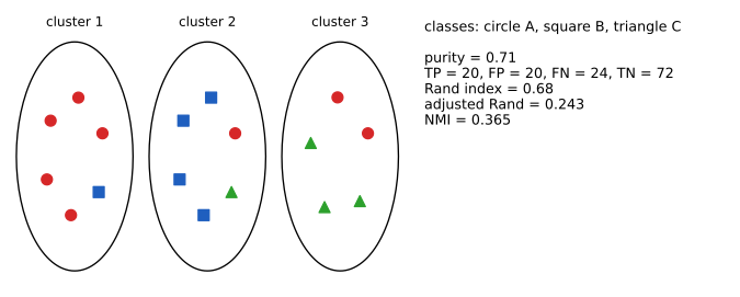
p. 716 With \(p_{ij}=N_{ij}/a_i\) the class distribution inside cluster \(i\), \[ \text{purity}=\sum_i\frac{a_i}{N}\max_jp_{ij}=\frac1N\sum_i\max_jN_{ij}. \tag{21.1} \] For the three clusters of Figure 21.1 (counts \(5,1,0\); \(1,4,1\); \(2,0,3\)) this is \((5+4+3)/17=12/17=0.71\) (21.2). Purity is between 0 and 1 but is trivially 1 when every object is its own cluster, so it ignores the number of clusters.
21.1.1.2 Rand index
pp. 716–717 Count the pairs of objects. TP: together in both \(U\) and \(V\); FP: together in \(U\) only; FN: together in \(V\) only; TN: apart in both. The Rand index is \[ R=\frac{TP+TN}{TP+FP+FN+TN}, \tag{21.3} \] the fraction of pair decisions that agree with the reference. In terms of the table: \(TP=\sum_{ij}\binom{N_{ij}}2\), \(TP+FP=\sum_i\binom{a_i}2\), \(TP+FN=\sum_j\binom{b_j}2\). For Figure 21.1 the three clusters have 6, 6 and 5 points, so \(TP+FP=15+15+10=40\) (21.4), \(TP=10+6+3+1=20\) (21.5), the three classes have 8, 5 and 4 members, so \(TP+FN=28+10+6=44\) and \(FN=24\), \(TN=136-20-20-24=72\), and \(R=92/136=0.68\). The adjusted Rand index subtracts the value expected for two random partitions with the same cluster sizes and rescales, \[ \text{ARI}=\frac{\text{index}-\text{expected index}}{\max\text{ index}-\text{expected index}}, \tag{21.6} \] with index \(=\sum_{ij}\binom{N_{ij}}2\), and for Figure 21.1 it equals \(0.243\): most of the apparent agreement of \(R=0.68\) is what chance alone gives.
21.1.1.3 Mutual information
p. 717 With \(p_{UV}(i,j)=N_{ij}/N\), \(p_U(i)=a_i/N\), \(p_V(j)=b_j/N\), the mutual information of the two partitions is \[ I(U,V)=\sum_{i=1}^R\sum_{j=1}^Cp_{UV}(i,j)\log\frac{p_{UV}(i,j)}{p_U(i)p_V(j)}, \tag{21.7} \] which lies in \([0,\min\{H(U),H(V)\}]\), and the normalised mutual information is \[ \text{NMI}(U,V)=\frac{I(U,V)}{(H(U)+H(V))/2}\in[0,1]. \tag{21.8} \] Like purity, \(I\) is maximal for many tiny clusters (then \(H(U)\) is large and \(I=H(V)\)), which the normalisation by \(H(U)\) penalises.
Filling the gap 21.1: pair counts from the table, the expectation behind the ARI, and the bounds on \(I\) and NMI pp. 716–717, (21.3)–(21.8)
Derivation
Pair counts. A pair of distinct objects is together in both partitions exactly when both lie in the same cell \((i,j)\), so \(TP=\sum_{ij}\binom{N_{ij}}2\). Pairs together in \(U\) are those inside a row: \(s_U=\sum_i\binom{a_i}2=TP+FP\); likewise \(s_V=\sum_j\binom{b_j}2=TP+FN\). With \(P=\binom N2\) pairs in all, \[ TN=P-TP-FP-FN=P-s_U-s_V+TP,\qquad R=\frac{TP+TN}{P}=1+\frac{2\,TP-s_U-s_V}{P}. \] So for fixed margins the Rand index is an increasing affine function of \(TP\).
The expected index. Take the margins \(a,b\) as fixed and let \(V\) be a uniformly random relabelling (the hypergeometric model of the book: all tables with the given margins arise from random permutations of the object labels). For one fixed pair of objects, \(\Pr(\text{together in }U)=s_U/P\) and, by symmetry of the permutation, the pair is together in \(V\) with probability \(s_V/P\), independently of \(U\) (which is fixed). By linearity, \[ \E[TP]=P\cdot\frac{s_U}P\cdot\frac{s_V}P=\frac{s_Us_V}{P}. \] Because \(R\) is affine in \(TP\), \(\E[R]\) is obtained by substituting \(\E[TP]\), and rescaling gives (21.6). The maximum \(TP\) is taken as the average \(\tfrac12(s_U+s_V)\) (Hubert and Arabie, 1985); this convention makes the ARI equal to 1 for identical partitions and keeps it symmetric. Hence \[ \text{ARI}=\frac{\sum_{ij}\binom{N_{ij}}2-s_Us_V/P}{\tfrac12(s_U+s_V)-s_Us_V/P}. \] For Figure 21.1: \(s_U=40\), \(s_V=44\), \(P=136\): \((20-12.94)/(42-12.94)=0.243\).
Bounds on \(I\). \(I(U,V)=\KL(p_{UV}\,\|\,p_Up_V)\ge0\) with equality iff the partitions are independent (Gibbs' inequality). Also \(I(U,V)=H(U)-H(U\given V)\le H(U)\) since conditional entropy is non-negative, and symmetrically \(I\le H(V)\). Hence \(0\le I\le\min\{H(U),H(V)\}\le\tfrac12(H(U)+H(V))\), so \(\text{NMI}\in[0,1]\) (the case \(H(U)=H(V)=0\), both partitions trivial, is conventionally 1). If every object is its own cluster, \(H(U\given V)=0\) and \(I=H(V)\), the maximal value, while purity is 1: the two measures reward over-segmentation, which is why they are reported with the number of clusters or in adjusted form. \(\square\)
pair_counts reproduces TP = 20, FP = 20, FN = 24, TN = 72 for Figure 21.1, and adjusted_rand, nmi agree with scikit-learn. The adjusted Rand index is also reported in the hierarchical-linkage demo.21.2 Hierarchical agglomerative clustering
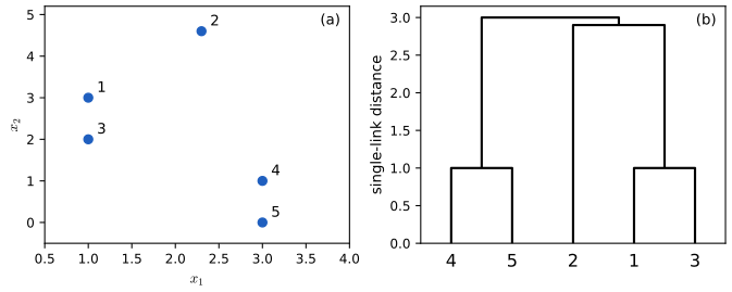
pp. 717–721 Hierarchical agglomerative clustering (HAC) takes a dissimilarity matrix \(D_{ij}\ge0\) and returns a binary tree (a dendrogram) whose leaves are the objects; cutting the tree at a height gives a nested family of clusterings. With the city-block distance \(d_{ij}=\sum_k|x_{ik}-x_{jk}|\) (21.9) on five points (Figure 21.2), points (1,3) and (4,5) are at distance 1 and merge first; the groups \(\{1,3\}\), \(\{4,5\}\), \(\{2\}\) are then compared by one of the group dissimilarities below.
See also: Elements of Statistical Learning, Section 14.3.12 and its gap 14.8 (invariance and what the three linkages estimate); Introduction to Statistical Learning, 12.4.2.
21.2.1 The algorithm
pp. 718–720
Algorithm 21.1: agglomerative clustering
- Start with singletons \(C_i=\{i\}\), \(i=1{:}N\), and the set of active clusters \(S=\{1,\dots,N\}\).
- Repeat until one cluster remains: pick \((j,k)=\arg\min_{j\ne k\in S}d_{jk}\); form \(C_\ell=C_j\cup C_k\); remove \(j,k\) from \(S\) and add \(\ell\); for every \(i\in S\) compute \(d(i,\ell)\) (the group dissimilarity).
The sequence of merge heights is the dendrogram. The three variants differ only in how \(d(i,\ell)\) is obtained. The demonstration Hierarchical linkage runs this algorithm in the browser.
21.2.1.1 Single link
pp. 719–720 The group dissimilarity is the smallest pair distance, \(d_{SL}(G,H)=\min_{i\in G,i'\in H}d_{ii'}\) (21.10). The tree is a minimum spanning tree of the data (Result 21.1), which is why single link can be run in \(O(N^2)\) time and why it follows chains of points.
21.2.1.2 Complete link
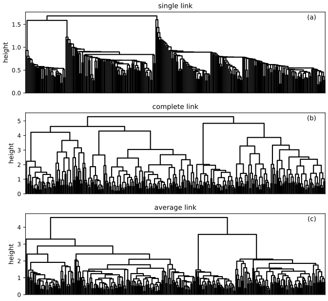
p. 720 \(d_{CL}(G,H)=\max_{i\in G,i'\in H}d_{ii'}\) (21.11). Two groups are close only if every pair across them is close, so the clusters have small diameter \(\max_{i,i'\in G}d_{ii'}\) (compact clusters); single link can build clusters of large diameter (Figure 21.4a against 21.4b).
21.2.1.3 Average link
p. 720 \(d_{avg}(G,H)=\frac1{n_Gn_H}\sum_{i\in G}\sum_{i'\in H}d_{ii'}\) (21.12), a compromise that tends to give compact, well separated groups; it is sensitive to the scale of \(d\), whereas single and complete link depend on \(d\) only through the ordering of its values.

Filling the gap 21.2: Result 21.1 (single link is a minimum spanning tree), the Lance-Williams update, no inversions, and invariance to monotone transforms pp. 719–720
Proof
(a) Lance-Williams updates. Suppose clusters \(j,k\) (sizes \(n_j,n_k\)) are merged into \(\ell\). Then for every other cluster \(i\): \[ \text{single: }d_{i\ell}=\min(d_{ij},d_{ik}),\quad\text{complete: }d_{i\ell}=\max(d_{ij},d_{ik}),\quad\text{average: }d_{i\ell}=\frac{n_jd_{ij}+n_kd_{ik}}{n_j+n_k}. \] The first two are immediate from the definitions of min and max over \(C_j\cup C_k\). For average link, \(\sum_{a\in C_i}\sum_{b\in C_\ell}d_{ab}=\sum_{a\in C_i}\sum_{b\in C_j}d_{ab}+\sum_{a\in C_i}\sum_{b\in C_k}d_{ab}=n_in_jd_{ij}+n_in_kd_{ik}\), and dividing by \(n_in_\ell=n_i(n_j+n_k)\) gives the weighted mean. So the algorithm needs only the matrix of group dissimilarities, updated in \(O(N)\) per merge.
(b) No inversions (monotone merge heights). Let \(h=d_{jk}\) be the minimum of the current dissimilarities, so every current dissimilarity is \(\ge h\). After the merge, the new entries \(d_{i\ell}\) are a minimum, a maximum, or a weighted mean of two numbers \(\ge h\), hence themselves \(\ge h\); the untouched entries are \(\ge h\). So the next minimum, the next merge height, is \(\ge h\). The heights are non-decreasing and the dendrogram can be drawn without crossings. (Centroid linkage does not have this property.)
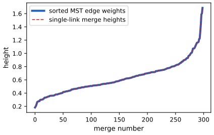
(c) Result 21.1. The merge heights of single link are the weights of the edges of a minimum spanning tree (MST) of the complete graph with weights \(d_{ij}\), in increasing order, and the merged pairs are the endpoints of those edges. At each step single link merges the two groups \(G,H\) with the smallest \(\min_{i\in G,i'\in H}d_{ii'}\), i.e. it adds the lightest edge joining two different current groups; as groups are the connected components of the edges added so far, no cycle is ever created. This is exactly Kruskal's algorithm. Kruskal's algorithm yields an MST by the cut property: if \(e\) is a lightest edge across a cut \((A,\bar A)\) and \(T\) is an MST not containing \(e\), then adding \(e\) to \(T\) creates a cycle which crosses the cut at another edge \(f\ne e\) with \(w(f)\ge w(e)\); \(T-f+e\) is a spanning tree of no greater weight, so some MST contains \(e\). The edge Kruskal adds joins two components \(G,H\) and is the lightest edge leaving \(G\) (every lighter edge from \(G\) goes inside a component already built), so by induction the edges chosen so far are contained in some MST. At the end the \(N-1\) chosen edges form a spanning tree contained in an MST, hence an MST. The merge height at step \(s\) is the weight of the \(s\)th chosen edge, and Kruskal chooses edges in non-decreasing weight order. \(\square\) (Figure 21.S1 shows the 299 merge heights of the 300 gene profiles and the sorted MST weights, which coincide.)
(d) Invariance. Let \(f\) be strictly increasing and apply it to every dissimilarity. Since \(\min(f(a),f(b))=f(\min(a,b))\) and \(\max(f(a),f(b))=f(\max(a,b))\), the updates (a) for single and complete link commute with \(f\): the matrix after any number of merges is \(f\) applied entrywise to the original sequence, and each step picks the same minimal pair. So the tree is unchanged and only the heights are transformed. Average link is not invariant, because \(f\) does not commute with the weighted mean. Example with three groups: after merging \(\{a,b\}\) suppose \(d(a,c)=1,\ d(b,c)=9\) and \(d(a,e)=d(b,e)=4\). The average distances are 5 to \(c\) and 4 to \(e\), so \(e\) is nearer. Under \(f(x)=x^{1/3}\) they become \((1+2.080)/2=1.540\) and \(4^{1/3}=1.587\), and now \(c\) is nearer. \(\square\)
Filling the gap 21.3: the running time of HAC p. 718, p. 720
Derivation
The book says that finding the closest pair costs \(O(N^2)\) per step and there are \(N-1\) steps, so the total is \(O(N^3)\), reduced to \(O(N^2\log N)\) with a priority queue; and that single link can be done in \(O(N^2)\) whereas the other variants "take \(O(N^3)\)". The first two statements are the cost of the naive and the heap implementations: with a heap of distances per active cluster, a merge deletes two heaps' worth of entries and inserts \(O(N)\) new distances at \(O(\log N)\) each, so a merge costs \(O(N\log N)\) and the total is \(O(N^2\log N)\) (plus \(O(N^2)\) to build the matrix). For single link, Result 21.1 reduces the problem to an MST, and Prim's algorithm on the dense graph costs \(O(N^2)\); sorting the \(N-1\) edges then gives the merge order. The last statement is correct for the straightforward implementation only. Complete and average link satisfy the reducibility property \(d(\ell,i)\ge\min(d(j,i),d(k,i))\) after merging a pair \(j,k\) (it holds for min, max and weighted means, all at least the smaller input), and for reducible linkages the nearest-neighbour-chain algorithm (Murtagh, 1983) also needs only \(O(N^2)\) time. So the \(O(N^3)\) quoted for them is not a lower bound. In every case the \(O(N^2)\) memory for the matrix remains, which is the real obstacle for large \(N\). \(\square\)
21.2.2 Example
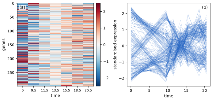
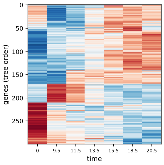
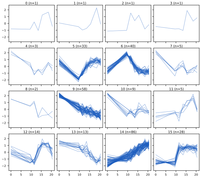
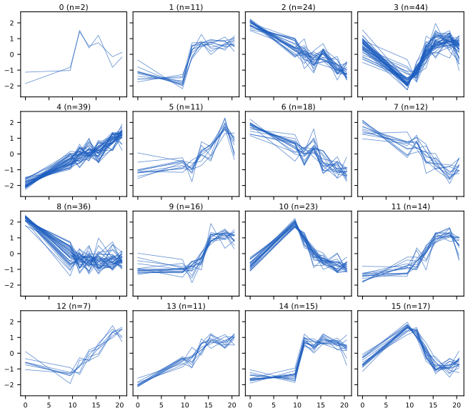
pp. 720–721 The book clusters \(N=300\) yeast genes measured at \(T=7\) time points (\(\bm x_n\in\R^7\), Figure 21.5): some genes rise over time, some fall, some have more complex responses. Using Euclidean distance and average link gives the dendrogram of Figure 21.6a (rows reordered by the tree), and cutting it at a suitable height gives 16 clusters whose time series look alike (Figure 21.6b). The yeast data are not available offline; I use 300 simulated profiles built from eight prototype shapes (the caption of Figure 21.5 says how), which reproduces the structure of the example. Here a cut into 16 average-link clusters gives clusters of very uneven size (the smallest are single genes: average link also merges outliers late), while the eight underlying shapes are better recovered by the cut at 8 (see the demonstration, preset 5).
21.2.3 Extensions
pp. 721–722 The book mentions a scalable parallel bottom-up algorithm (Monath et al. 2021) and an online algorithm that revisits earlier merging decisions and, under assumptions, provably recovers the true hierarchy (Monath et al. 2019), used for clustering mentions of entities in a text stream. These are research results cited without proof and are not developed here.
21.3 K means clustering
p. 722 HAC needs a dissimilarity matrix (\(O(N^2)\) memory, \(O(N^2\log N)\) time or worse), is an algorithm without an objective, and assumes the notion of similarity is given. K-means (MacQueen 1967, Lloyd 1982) takes data vectors, learns the \(K\) cluster centres \(\bm\mu_k\in\R^D\), runs in \(O(NKT)\) time for \(T\) iterations and minimises an explicit cost.
See also: Bayesian and Probabilistic ML, Section 9.1 and its gap 9.1 (why the two steps are exact minimisations); Elements of Statistical Learning, 14.3.6; Introduction to Statistical Learning, 12.4.1.
21.3.1 The algorithm
p. 722 Assign each point to its nearest centre, then move each centre to the mean of its points, and repeat: \[ z_n^*=\arg\min_k\|\bm x_n-\bm\mu_k\|_2^2,\qquad \bm\mu_k=\frac1{n_k}\sum_{n:z_n=k}\bm x_n. \tag{21.13, 21.14} \] These two steps alternately minimise the distortion (inertia, within-cluster sum of squares) \[ J(\bm M,\bm Z)=\sum_{n=1}^N\|\bm x_n-\bm\mu_{z_n}\|^2=\|\bm X-\bm Z\bm M^\T\|_F^2, \tag{21.15} \] where \(\bm X\in\R^{N\times D}\), \(\bm M\in\R^{D\times K}\) holds the centres in its columns and \(\bm Z\in\{0,1\}^{N\times K}\) is the one-hot matrix of assignments (the book writes \([0,1]\); the identity needs entries 0 or 1, see the notes on the book).
Filling the gap 21.4: the two steps are exact minimisations, the distortion decreases, the algorithm stops, and the identities behind (21.15) p. 722, (21.13)–(21.15)
Proof
(a) Centre step. For a fixed cluster \(S\) of \(n_S\) points with mean \(\bar{\bm x}\) and any \(\bm\mu\), \(\sum_{n\in S}\|\bm x_n-\bm\mu\|^2=\sum_{n\in S}\|\bm x_n-\bar{\bm x}\|^2+n_S\|\bar{\bm x}-\bm\mu\|^2\) (the cross term \(2(\bar{\bm x}-\bm\mu)^\T\sum(\bm x_n-\bar{\bm x})\) vanishes). So the mean is the unique minimiser, which is (21.14), and moving a centre to the mean of its points can only lower \(J\).
(b) Assignment step. \(J=\sum_n\|\bm x_n-\bm\mu_{z_n}\|^2\) is a sum of terms, each depending on its own \(z_n\); each is smallest when \(z_n\) is the nearest centre, (21.13).
(c) Descent and termination. Let \(J_t\) be the distortion after the assignment step of round \(t\) and \(J_t'\) after the following centre step. By (b), (a): \(J_{t+1}\le J_t'\le J_t\). The number of partitions of \(N\) points into \(K\) labelled groups is finite (\(K^N\)). A partition cannot repeat unless the algorithm has stopped: if the assignment step returns the same labels as before, the centres computed next equal the current ones, so nothing changes any more; if it returns different labels without a tie, then \(J\) has decreased strictly or stayed equal only if every point moved to an equally near centre (a tie), and breaking ties by a fixed rule (smallest index) avoids cycling. So a partition never reappears, and after finitely many rounds the labels stop changing. The limit is a fixed point: the centres are the means of their clusters and the clusters are the Voronoi cells of the centres.
(d) What kind of minimum. \(J(\bm M)=\sum_n\min_k\|\bm x_n-\bm\mu_k\|^2\) is piecewise quadratic in the centres. At a fixed point with no data point equidistant from two centres, the assignment is locally constant in \(\bm M\), so \(J\) coincides near the fixed point with the quadratic \(\sum_k\sum_{n\in S_k}\|\bm x_n-\bm\mu_k\|^2\), which by (a) is minimised at the means: a local minimum. It need not be global: the objective is not convex (Figure 21.7b), and finding the global minimum is NP-hard even in the plane (cited result).
(e) The identities. With \(\bm Z\) one-hot, row \(n\) of \(\bm Z\bm M^\T\) is \(\bm\mu_{z_n}^\T\), so \(\|\bm X-\bm Z\bm M^\T\|_F^2=\sum_n\|\bm x_n-\bm\mu_{z_n}\|^2\); for a general \(\bm Z\in[0,1]^{N\times K}\) it would not equal (21.15). Expanding the squares for cluster \(S\) with mean \(\bar{\bm x}\), \[ \frac1{2n_S}\sum_{i,j\in S}\|\bm x_i-\bm x_j\|^2=\frac1{2n_S}\sum_{i,j}\big(\|\bm x_i-\bar{\bm x}\|^2+\|\bm x_j-\bar{\bm x}\|^2\big)=\sum_{i\in S}\|\bm x_i-\bar{\bm x}\|^2, \] so the distortion is also \(\sum_k\frac1{2n_k}\sum_{i,j\in S_k}\|\bm x_i-\bm x_j\|^2\), which depends on the data only through pairwise distances. Finally the total sum of squares splits as \(\sum_n\|\bm x_n-\bar{\bm x}\|^2=J+\sum_kn_k\|\bm\mu_k-\bar{\bm x}\|^2\) (within plus between). \(\square\)
21.3.2 Examples
pp. 722–724
21.3.2.1 Clustering points in the 2d plane
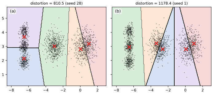
p. 723 K-means induces a Voronoi tessellation of the plane (each cell is the set of points nearer to one centre than to the others), and the solution depends on the initialisation: of two random starts, the one with the larger distortion is worse (Figure 21.7). In scikit-learn the distortion is called inertia, and the default is ten restarts combined with K-means++ seeding (Section 21.3.4), keeping the lowest-distortion run.
21.3.2.2 Clustering gene expression time series data from yeast cells
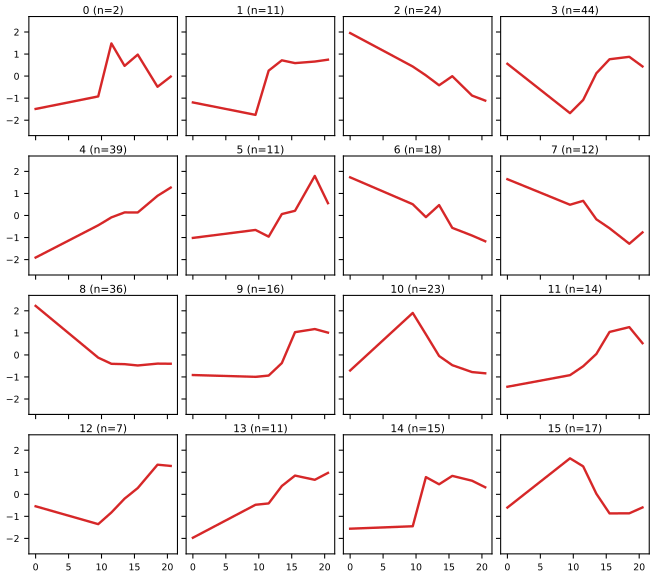
pp. 723–724 K-means with \(K=16\) on the gene profiles groups similar series, and each centre is a reasonable prototype (Figure 21.8). The book's run leaves one cluster empty, an accident of the initialisation; implementations then restart the empty cluster at the worst-fitted point, as the code does.
21.3.3 Vector quantization
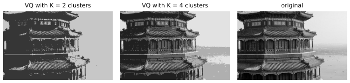
pp. 724–725 Vector quantisation (VQ) encodes a vector \(\bm x_n\in\R^D\) by the index of its nearest prototype in a codebook of \(K\) vectors, \[ \operatorname{encode}(\bm x_n)=\arg\min_k\|\bm x_n-\bm\mu_k\|^2,\qquad J=\frac1N\sum_n\|\bm x_n-\operatorname{decode}(\operatorname{encode}(\bm x_n))\|^2=\frac1N\sum_n\|\bm x_n-\bm\mu_{z_n}\|^2, \tag{21.16, 21.17} \] with \(\operatorname{decode}(k)=\bm\mu_k\): the cost minimised by K-means (divided by \(N\)). Storing \(N\) vectors with \(B\) bits per scalar costs \(NDB\) bits; the VQ code costs \(N\log_2K+KDB\) bits.
Filling the gap 21.6: the bit counts and the image example pp. 724–725
Derivation
Each of the \(N\) vectors needs an index in \(\{1,\dots,K\}\), which a fixed-length code writes with \(\lceil\log_2K\rceil\) bits (exactly \(\log_2K\) when \(K\) is a power of two): \(N\log_2K\) bits. The codebook has \(K\) entries of \(D\) scalars of \(B\) bits: \(KDB\) bits. Total \(N\lceil\log_2K\rceil+KDB\), against \(NDB\) uncompressed. When \(N\gg KDB/\log_2K\), the second term is negligible and the rate per vector is \(\log_2K\) bits against \(DB\), a compression factor \(DB/\log_2K\). For the \(200\times320\) image, \(D=1\) (each pixel is a scalar, \(N=64{,}000\)) and \(B=8\): the raw size is \(512{,}000\) bits. With \(K=4\): \(64{,}000\cdot2+4\cdot8=128{,}032\) bits, a factor \(3.998\approx4\), as the book says (about 128 kb); with \(K=2\), \(64{,}032\) bits, a factor 8. The cost in quality is the distortion: on the image of Figure 21.9 the mean squared error per pixel (the distortion (21.17)) is 1042 for \(K=2\) (root mean square 32 grey levels) and 280 for \(K=4\) (16.7 levels). Zero distortion needs \(K=N\) with \(\bm\mu_n=\bm x_n\), which does not compress. The book's remark that modelling the correlation between neighbouring pixels (as JPEG does with blocks) would shrink the residual and the code is the link between compression and density estimation: an ideal code spends \(-\log_2p(\bm x)\) bits on \(\bm x\), and an entropy code for the indices uses \(H\le\log_2K\) bits per pixel, which is smaller when the clusters have unequal sizes. \(\square\)
21.3.4 The K-means++ algorithm
p. 725 Because the objective is non-convex, initialisation matters. K-means++ picks the first centre uniformly at random among the data points and each further centre \(\bm\mu_t=\bm x_n\) with probability \[ p(\bm\mu_t=\bm x_n)=\frac{D_{t-1}(\bm x_n)}{\sum_{n'}D_{t-1}(\bm x_{n'})},\qquad D_{t-1}(\bm x)=\min_{k=1}^{t-1}\|\bm x-\bm\mu_k\|_2^2, \tag{21.18, 21.19} \] so that far-away points are likely to become centres. (The book's (21.18) writes \(D_{t-1}\) in the numerator without saying that it is the squared distance of (21.19); that is what is meant.) Arthur and Vassilvitskii (2007) proved that the expected distortion of the seeding is at most \(O(\log K)\) times the optimum.
Filling the gap 21.7: the \(O(\log K)\) guarantee of K-means++ (Arthur and Vassilvitskii) p. 725, [AV07]
Proof
Setup. For a set of centres \(\mathcal C\) write \(\phi(\mathcal C;S)=\sum_{\bm x\in S}\min_{\bm c\in\mathcal C}\|\bm x-\bm c\|^2\) and \(\phi(\mathcal C)=\phi(\mathcal C;X)\). Let \(A_1,\dots,A_K\) be the clusters of an optimal solution, with means \(\bm c(A_i)\), and \(\phi_{OPT}(A)=\sum_{\bm x\in A}\|\bm x-\bm c(A)\|^2\), \(\phi_{OPT}=\sum_i\phi_{OPT}(A_i)\). Seeding with \(K\) centres then costs \(\phi(\mathcal C)\). The claim is \(\E[\phi(\mathcal C)]\le8(\ln K+2)\,\phi_{OPT}\).
Lemma A (one uniform centre). If \(\bm a\) is drawn uniformly from \(A\), \(\E[\phi(\{\bm a\};A)]=2\phi_{OPT}(A)\). Proof: with \(\bm c=\bm c(A)\), \(\|\bm x-\bm a\|^2=\|\bm x-\bm c\|^2+\|\bm a-\bm c\|^2+2(\bm x-\bm c)^\T(\bm c-\bm a)\); summing over \(\bm x\in A\) kills the cross term, giving \(\phi_{OPT}(A)+|A|\|\bm a-\bm c\|^2\); averaging over \(\bm a\) gives \(\phi_{OPT}(A)+\phi_{OPT}(A)\).
Lemma B (one \(D^2\)-sampled centre). Let \(\mathcal C\) be any non-empty set of centres, \(D(\bm x)\) the distance to the nearest, and \(A\) a cluster. If \(\bm a_0\) is drawn from \(A\) with probability \(D(\bm a_0)^2/\sum_{\bm a\in A}D(\bm a)^2\), then \(\E[\phi(\mathcal C\cup\{\bm a_0\};A)]\le8\phi_{OPT}(A)\). Proof: by definition \[ \E=\sum_{\bm a_0\in A}\frac{D(\bm a_0)^2}{\sum_{\bm a}D(\bm a)^2}\sum_{\bm x\in A}\min\big(D(\bm x),\|\bm x-\bm a_0\|\big)^2. \] By the triangle inequality \(D(\bm a_0)\le D(\bm a)+\|\bm a-\bm a_0\|\) for every \(\bm a\in A\), so \(D(\bm a_0)^2\le2D(\bm a)^2+2\|\bm a-\bm a_0\|^2\); averaging over \(\bm a\in A\): \(D(\bm a_0)^2\le\frac2{|A|}\sum_{\bm a}D(\bm a)^2+\frac2{|A|}\sum_{\bm a}\|\bm a-\bm a_0\|^2\). Insert this in the numerator. The first part gives \(\frac2{|A|}\sum_{\bm a_0}\sum_{\bm x}\min(\cdot)^2\le\frac2{|A|}\sum_{\bm a_0}\sum_{\bm x}\|\bm x-\bm a_0\|^2=4\phi_{OPT}(A)\) by Lemma A (use \(\min\le\|\bm x-\bm a_0\|\)); the denominator cancelled with \(\sum_{\bm a}D(\bm a)^2\). In the second part use \(\min(D(\bm x),\|\bm x-\bm a_0\|)^2\le D(\bm x)^2\) so that \(\sum_{\bm x}\min(\cdot)^2\le\sum_{\bm x}D(\bm x)^2\), which cancels the denominator, leaving \(\frac2{|A|}\sum_{\bm a_0}\sum_{\bm a}\|\bm a-\bm a_0\|^2=4\phi_{OPT}(A)\). Total \(\le8\phi_{OPT}(A)\).
Lemma C (induction). Let \(\mathcal C\) be arbitrary and choose \(u>0\) optimal clusters as "uncovered" with union \(X_u\); \(X_c\) is the rest. Add \(t\le u\) centres by \(D^2\)-sampling, obtaining \(\mathcal C'\). Then \[ \E[\phi(\mathcal C')]\le\big(\phi(X_c)+8\phi_{OPT}(X_u)\big)(1+H_t)+\frac{u-t}{u}\phi(X_u), \qquad H_t=1+\tfrac12+\dots+\tfrac1t, \] where \(\phi(X)\) means the cost under \(\mathcal C\) and \(\phi_{OPT}(X_u)\) is the sum of the optimal costs of the uncovered clusters. Proof by induction on \((t,u)\). Case \(t=0\): the right side is \(\phi(X_c)+8\phi_{OPT}(X_u)+\phi(X_u)\ge\phi(\mathcal C)\). Case \(t=u=1\): with probability \(\phi(X_c)/\phi\) the new centre is in \(X_c\) and the cost does not increase (\(\le\phi\)); with probability \(\phi(X_u)/\phi\) it lies in an uncovered cluster, and by Lemma B the expected cost of that cluster becomes at most \(8\phi_{OPT}(A)\), so the total is at most \(\phi(X_c)+8\phi_{OPT}(X_u)\). Combining, \(\E\le\phi(X_c)+8\phi_{OPT}(X_u)+\frac{\phi(X_c)}{\phi}\phi(X_u)\le2\phi(X_c)+8\phi_{OPT}(X_u)\), which is the bound with \(1+H_1=2\). Step: let \(t\ge1\), \(u\ge1\), not both 1 (so \(u\ge2\) when \(t=1\)), and assume the lemma for \((t-1,u)\) and \((t-1,u-1)\). The first new centre falls in \(X_c\) with probability \(\phi(X_c)/\phi\) (\(\phi=\phi(X_c)+\phi(X_u)\)): the costs do not increase, and the \((t-1,u)\) bound gives at most \((\phi(X_c)+8\phi_{OPT}(X_u))(1+H_{t-1})+\frac{u-t+1}u\phi(X_u)\). It falls in an uncovered cluster \(A\) with probability \(\phi(A)/\phi\): the cluster becomes covered, with expected cost \(\le8\phi_{OPT}(A)\) (Lemma B), and the \((t-1,u-1)\) bound gives at most \((\phi(X_c)+8\phi_{OPT}(X_u))(1+H_{t-1})+\frac{u-t}{u-1}(\phi(X_u)-\phi(A))\). Averaging over \(A\) with weights \(\phi(A)/\phi(X_u)\), and using \(\sum_A\phi(A)^2\ge\phi(X_u)^2/u\) (power-mean inequality), so that \(\sum_A\frac{\phi(A)}{\phi(X_u)}(\phi(X_u)-\phi(A))\le\phi(X_u)\frac{u-1}u\), this case is at most \((\phi(X_c)+8\phi_{OPT}(X_u))(1+H_{t-1})+\frac{u-t}u\phi(X_u)\). Hence the overall expectation is at most \[ (\phi(X_c)+8\phi_{OPT}(X_u))(1+H_{t-1})+\frac{\phi(X_c)}{\phi}\frac{u-t+1}u\phi(X_u)+\frac{\phi(X_u)}\phi\frac{u-t}u\phi(X_u). \] The target exceeds this by \(\frac1t(\phi(X_c)+8\phi_{OPT}(X_u))+\frac{u-t}u\phi(X_u)\big[1-\frac{\phi(X_c)+\phi(X_u)}{\phi}\big]-\frac{\phi(X_c)\phi(X_u)}{u\phi}\) (using \(1+H_t-(1+H_{t-1})=\frac1t\)). The bracket is 0, so the excess is \(\ge\frac{\phi(X_c)}t-\frac{\phi(X_c)}u\cdot\frac{\phi(X_u)}\phi\ge\phi(X_c)(\frac1t-\frac1u)\ge0\) because \(t\le u\). \(\square\)
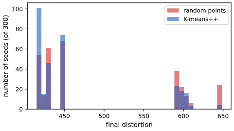
The theorem. The first centre is uniform; suppose it lies in the optimal cluster \(A\). By Lemma A, \(\E\phi(A)=2\phi_{OPT}(A)\) after the first centre. Apply Lemma C with \(X_c=A\), \(u=t=K-1\), noting that the other \(K-1\) centres are \(D^2\)-sampled (the covered cluster only helps): \(\E[\phi]\le(2\phi_{OPT}(A)+8(\phi_{OPT}-\phi_{OPT}(A)))(1+H_{K-1})\le8\phi_{OPT}(1+H_{K-1})\le8(2+\ln K)\phi_{OPT}\), since \(H_{K-1}\le1+\ln(K-1)\). Averaging over the choice of \(A\) keeps the bound. Lloyd's iterations afterwards can only lower the cost. \(\square\) (The guarantee is on the expected cost and its constant is pessimistic. Figure 21.S2: over 300 seeds the final distortion of K-means++ has a lower mean than random seeding, 465 against 492, and more runs end near the best value.)
21.3.5 The K-medoids algorithm
pp. 725–726 K-medoids restricts each centre to be a data point, the medoid of its cluster: the member with the smallest sum of dissimilarities to the other members. It needs only the \(N\times N\) distance matrix, so it applies to objects where averaging makes no sense, and it is more robust to outliers than the mean. The classical algorithm is partitioning around medoids (PAM): try swapping each medoid with each non-medoid and keep a swap that lowers the cost; this costs \(O(N^2KT)\) for \(T\) passes. The simpler Voronoi iteration of Park and Jun (2009) alternates assigning \(z_n=\arg\min_kd(n,m_k)\) and recomputing the medoid of each cluster (Algorithm 21.2).
Algorithm 21.2: K-medoids (Voronoi iteration)
- Initialise \(m_{1:K}\) as a random subset of size \(K\) of \(\{1,\dots,N\}\).
- Repeat until convergence: \(z_n=\arg\min_kd(n,m_k)\) for all \(n\); then \(m_k=\arg\min_{n:z_n=k}\sum_{n':z_{n'}=k}d(n,n')\) for all \(k\).
Filling the gap 21.8: Voronoi-iteration K-medoids decreases the cost and stops; PAM; the cost of the medoid step pp. 725–726, Algorithm 21.2
Proof
The cost is \(C(\bm z,\bm m)=\sum_nd(n,m_{z_n})\). For fixed medoids the assignment \(z_n=\arg\min_kd(n,m_k)\) minimises each term, so it minimises \(C\). For a fixed assignment, \(C=\sum_k\sum_{n\in S_k}d(n,m_k)\) separates over clusters, and \(m_k\) ranges over all points in \(\{1,\dots,N\}\); restricting to members of \(S_k\) (as the algorithm does) finds the minimiser among members, which is an upper bound for the unrestricted minimiser and, the cost not increasing, still yields \(C\) non-increasing: \(C_{t+1}\le C_t'\le C_t\). Finiteness of the number of assignments and a fixed tie rule give termination at a fixed point, as in gap 21.4. The medoid step costs \(\sum_k|S_k|^2\le N^2\) distance look-ups per pass, i.e. \(O(N^2)\), and the assignment step \(O(NK)\); PAM, which examines \(K(N-K)\) swaps each costing \(O(N)\) to evaluate, takes \(O(KN^2)\) per pass, \(O(N^2KT)\) in all, as the book states. Every accepted swap strictly lowers the cost, so PAM also stops, at a configuration no single swap improves, which is at least as good as a Voronoi fixed point started from the same medoids (checked on random data in the code). Relation to K-means: with \(d=\|\cdot\|^2\) the cost with medoids restricted to data points is never below the K-means distortion for the same partition, because by gap 21.4(a) the mean is the unconstrained minimiser; the price of robustness is a larger cost and a discrete search. \(\square\)
21.3.6 Speedup tricks
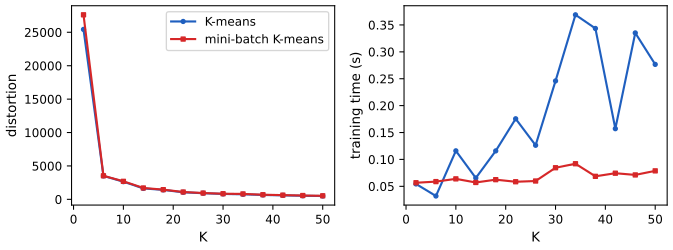
p. 726 The cost \(O(NKI)\) for \(I\) iterations can be reduced in the constant: Elkan (2003) uses the triangle inequality to keep lower and upper bounds on point-to-centre distances and skip most distance computations (the clusters found are identical); the mini-batch variant of Sculley (2010) updates each centre by a running average with a per-centre rate \(1/(\text{number absorbed})\) from small random batches. It is much faster but gives a slightly larger distortion (Figure 21.10).
21.3.7 Choosing the number of clusters K
pp. 726–729
21.3.7.1 Minimizing the distortion
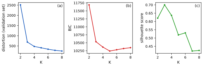
p. 727 A supervised-learning reflex would be to pick the \(K\) with the smallest validation reconstruction error \(\text{err}(\mathcal D_{valid},K)=\frac1{|\mathcal D_{valid}|}\sum_n\|\bm x_n-\hat{\bm x}_n\|_2^2\) (21.20). It does not work: the error keeps falling as \(K\) grows (Figure 21.11a), because K-means is a degenerate density model of \(K\) spikes, and more spikes cover the space better.
Filling the gap 21.9: why the distortion always falls with K, and what is true on a validation set p. 727, (21.20)
Derivation
Training distortion. Let \(J_K^*=\min_{\bm M,\bm z}J\) over \(K\) centres. Given an optimal \(K\)-codebook, adding any \((K+1)\)th centre cannot raise any point's distance to its nearest centre, so \(J^*_{K+1}\le J_K^*\). With distinct points \(J_N^*=0\) (a centre on every point). So the optimal training distortion is non-increasing, and hitting zero at \(K=N\), it cannot identify a "best" \(K\) by being minimal: its minimiser is \(K=N\). Lloyd's algorithm finds local minima, so the observed curve of fitted distortions is only approximately monotone (restarts help).
Population distortion. For a distribution \(P\) on a compact set, the optimal \(K\)-point quantiser has distortion \(D_K^*=\min_{|\mathcal C|=K}\E\min_{\bm c}\|\bm x-\bm c\|^2\), non-increasing by the same argument, and \(D_K^*\to0\) as \(K\to\infty\): cover the support by a finite grid of mesh \(\epsilon\) (a number of cells that grows like \(\epsilon^{-D}\)), take the cell centres as the codebook: the distortion is at most \(\epsilon^2\). Zador's theorem (cited) gives the rate \(D_K^*\asymp K^{-2/D}\) for a density in \(\R^D\). So even the true out-of-sample criterion favours ever larger \(K\), with no interior minimum.
A validation set. For a codebook fitted on a finite training set and scored on fresh data the error is not guaranteed to be monotone, only to follow the downward trend. In a numerical experiment (25 training points and 2000 validation points from a standard bivariate normal, \(K=1,\dots,12\)) the validation curve rose at some step in 14 of 40 runs: the book's "monotonically decreases" is a statement about the trend and about the large-\(N\) case, as in Figure 21.11a, where both the training and validation sets are large and the curve is monotone. Either way the conclusion stands: unlike prediction error, held-out reconstruction error is not a model-selection criterion for clusters, and the same holds for choosing the dimension in PCA (Section 20.1.4). \(\square\)
21.3.7.2 Maximizing the marginal likelihood
p. 728 A probabilistic model such as a Gaussian mixture (Section 21.4.1) allows the log marginal likelihood to be used, approximated by the BIC (Section 5.2.5.1): \[ \text{BIC}(K)=\log p(\mathcal D\given\hat{\bm\theta}_K)-\frac{d_K}2\log N, \tag{21.21} \] with \(d_K\) the number of free parameters. Plotted in the common software convention (minus twice this), BIC is U-shaped in \(K\) (Figure 21.11b): each Gaussian fills a volume of space instead of being a spike, so once the real modes are covered the Occam factor penalises more components.
Filling the gap 21.11: BIC as the Laplace approximation, the parameter counts, and the sign convention p. 728, (21.21), Section 5.2.5.1
Derivation
Laplace approximation. The marginal likelihood is \(p(\mathcal D)=\int e^{\ell(\bm\theta)}p(\bm\theta)\,d\bm\theta\) with \(\ell(\bm\theta)=\log p(\mathcal D\given\bm\theta)\), a sum of \(N\) terms. Expand around the maximiser \(\hat{\bm\theta}\): \(\ell(\bm\theta)\approx\ell(\hat{\bm\theta})-\frac12(\bm\theta-\hat{\bm\theta})^\T\bm H(\bm\theta-\hat{\bm\theta})\), with \(\bm H=-\nabla^2\ell(\hat{\bm\theta})=N\hat{\bm I}_1\), where \(\hat{\bm I}_1\) is the average observed information per observation (positive definite for a regular model with \(d\) free parameters). With a smooth prior that is nearly constant near \(\hat{\bm\theta}\), the Gaussian integral gives \[ \log p(\mathcal D)\approx\ell(\hat{\bm\theta})+\log p(\hat{\bm\theta})+\frac d2\log2\pi-\frac12\log|N\hat{\bm I}_1|=\ell(\hat{\bm\theta})-\frac d2\log N+O(1), \] since \(\log|N\hat{\bm I}_1|=d\log N+\log|\hat{\bm I}_1|\) and the remaining terms do not grow with \(N\). This is (21.21). Common software reports \(-2\) times it, \(\text{BIC}=-2\ell(\hat{\bm\theta})+d\log N\), to be minimised; the plot of Figure 21.11b is in that convention (the book's (21.21) is to be maximised).
Caveat for mixtures. A mixture is not a regular model: it is non-identifiable (gap 21.13), and the likelihood is unbounded for full covariances (gap 21.12), so the Laplace argument holds only heuristically (it is rigorous for BIC consistency in restricted settings, and Watanabe's singular learning theory replaces \(d/2\) by a smaller "learning coefficient"). The BIC is used in practice as a consistent-in-practice guide, and the book's Figure 21.11b shows that it works on this example.
Parameter counts for a \(K\)-component mixture of Gaussians in \(\R^D\): mixing weights \(K-1\), means \(KD\), plus the covariances: full \(K\,D(D+1)/2\); tied (one shared full matrix) \(D(D+1)/2\); diagonal \(KD\); spherical \(K\). For \(D=2\), \(K=5\): full 29, tied 17, diagonal 24, spherical 19. With these counts the BIC values of the five-component fits to the data of Figure 21.14 are 6982, 7401, 7378 and 7544 (full, tied, diagonal, spherical), selecting the full covariance model, as the pictures suggest. \(\square\)
21.3.7.3 Silhouette coefficient
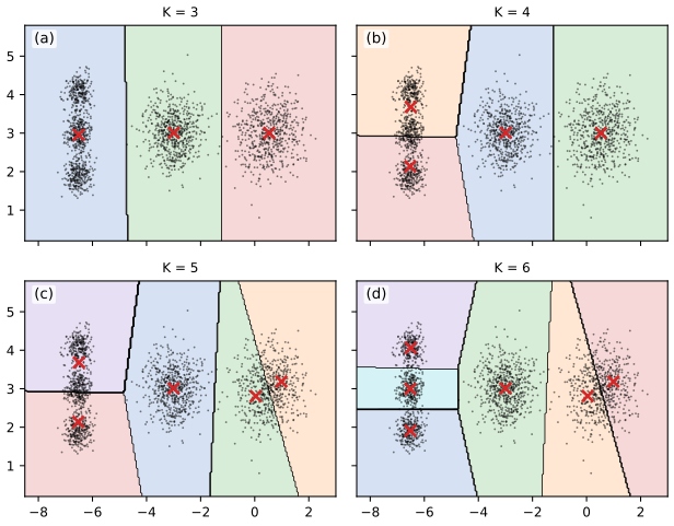
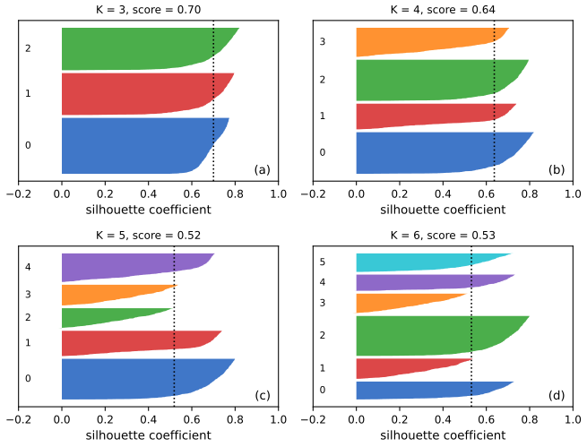
p. 728 The silhouette is a heuristic for spherical clusters. For instance \(i\) let \(a_i\) be the mean distance to the other members of its own cluster (compactness) and \(b_i\) the mean distance to the members of the next closest cluster (separation), and \[ sc(i)=\frac{b_i-a_i}{\max(a_i,b_i)}\in[-1,1]. \] Values near \(+1\) mean the point is close to its cluster and far from others, near 0 mean it is on a boundary, near \(-1\) mean it is probably in the wrong cluster. The silhouette score of a clustering is the mean of \(sc(i)\). On the blob data the score peaks at \(K=3\) (0.70) with a second bump at \(K=5,6\), while the distortion has only a faint elbow (Figure 21.11). The silhouette diagram (Figure 21.13) shows the coefficients of each cluster sorted, so that thin clusters and clusters with many points below the average line stand out; it also shows cluster sizes in any dimension.
Filling the gap 21.10: range, invariances and the two definitions of the silhouette p. 728
Derivation
Range. \(a_i,b_i\ge0\) are averages of distances, so \(|b_i-a_i|\le\max(a_i,b_i)\) (the difference of two non-negative numbers is at most the larger), giving \(sc(i)\in[-1,1]\). \(sc(i)=1\) iff \(a_i=0<b_i\) (all other members of the cluster coincide with \(\bm x_i\)); \(sc(i)=0\) iff \(a_i=b_i\); \(sc(i)=-1\) iff \(b_i=0<a_i\). For a singleton cluster \(a_i\) is undefined and the convention is \(sc(i)=0\). The score needs \(2\le K\le N-1\).
Invariances. Scaling all coordinates by \(\lambda>0\) multiplies \(a_i\) and \(b_i\) by \(\lambda\), so the coefficient is unchanged; it is also unchanged by translations and rotations (distances are). It is not invariant to a change of the distance, so the choice of metric (and standardisation of features) matters.
Which "next closest" cluster. The standard definition (and the code here, and scikit-learn) takes \(b_i=\min_{k\ne k_i}\) of the mean distance from \(\bm x_i\) to the points of cluster \(k\). The book defines the next closest cluster by the nearest centroid, \(k_i'=\arg\min_{k\ne k_i}\|\bm\mu_k-\bm x_i\|\), and \(b_i\) as the mean distance to that cluster. The two agree when the nearest centroid and the nearest cluster in mean distance coincide, which is the case for round, well separated clusters; they can differ for elongated or unequal clusters. On the blob data with \(K=4\) the two scores differ by less than 0.02. Also, the book's \(k_i=\arg\min_k\|\bm\mu_k-\bm x_i\|\) assigns the cluster by nearest centroid, which for a K-means solution is the cluster label itself. \(\square\)
21.3.7.4 Incrementally growing the number of mixture components
pp. 728–729 One can start with a small \(K\), and after each training round split the component with the largest mixing weight into two (new centres are random perturbations of the old centre, each with half the weight), removing components whose weight or variance becomes too small, until the desired number is reached (Figueiredo and Jain 2002). The method is cited and not analysed in the book.
21.3.7.5 Sparse estimation methods
p. 729 Alternatively choose a large \(K\) and use a sparsity-promoting prior (for example a Dirichlet prior on the weights with a small concentration) or variational inference to switch off unneeded components; the book defers the details to its sequel.
21.4 Clustering using mixture models
p. 729 K-means assumes spherical clusters of equal size and applies only to vectors in \(\R^D\). A mixture model (Section 3.5) removes both restrictions: different covariance shapes, and other component families such as Bernoulli distributions for binary data.
See also: Bayesian and Probabilistic ML, Section 9.2 (mixtures of Gaussians) with the EM derivation in 9.2.2, and the demo mixture densities.
21.4.1 Mixtures of Gaussians
p. 730 A Gaussian mixture model (GMM) has density \(p(\bm x\given\bm\theta)=\sum_{k=1}^K\pi_k\N(\bm x\given\bm\mu_k,\bm\Sigma_k)\) (21.22). Given parameters, the posterior probability of cluster \(k\) for point \(\bm x_n\), the responsibility, is \[ r_{nk}=p(z_n=k\given\bm x_n,\bm\theta)=\frac{\pi_k\N(\bm x_n\given\bm\mu_k,\bm\Sigma_k)}{\sum_{k'}\pi_{k'}\N(\bm x_n\given\bm\mu_{k'},\bm\Sigma_{k'})}, \tag{21.23} \] and the most probable assignment (hard clustering) is \[ \hat z_n=\arg\max_kr_{nk}=\arg\max_k\big[\log p(\bm x_n\given z_n=k,\bm\theta)+\log p(z_n=k\given\bm\theta)\big]. \tag{21.24} \] The second equality holds because the denominator of (21.23) does not depend on \(k\).
21.4.1.1 K-means is a special case of EM
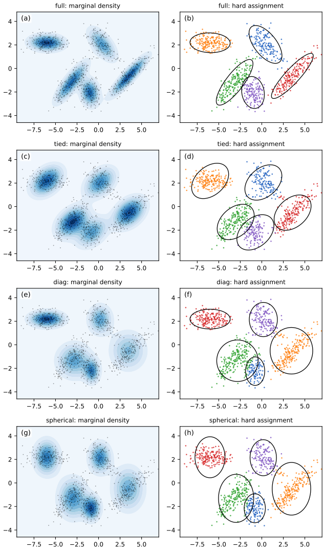
pp. 730–731 EM for a GMM (Section 8.7.3) alternates computing the responsibilities (E step) and weighted maximum-likelihood updates (M step). K-means arises with two approximations: the covariances are fixed at \(\bm\Sigma_k=\bm I\) and the weights at \(\pi_k=1/K\), and the E step is made hard, \(r_{nk}\approx\mathbb I(k=z_n^*)\). The weighted MLE of the means then reduces to (21.14). The restriction to spherical clusters is severe: Figure 21.14 fits \(K=5\) components with full, tied, diagonal and spherical covariances to 2-D data and only the full model captures the correlated clusters.
Filling the gap 21.5: K-means as the small-variance, hard-assignment limit of EM pp. 730–731
Derivation
EM updates for a GMM (Section 8.7.3). With responsibilities \(r_{nk}\) and \(N_k=\sum_nr_{nk}\), the M step is \(\pi_k=N_k/N\), \(\bm\mu_k=\frac1{N_k}\sum_nr_{nk}\bm x_n\), \(\bm\Sigma_k=\frac1{N_k}\sum_nr_{nk}(\bm x_n-\bm\mu_k)(\bm x_n-\bm\mu_k)^\T\) (derivations in the companion course).
Limit \(\sigma^2\to0\). Take \(\pi_k=1/K\) and \(\bm\Sigma_k=\sigma^2\bm I\) fixed. Then \[ r_{nk}=\frac{\exp(-\|\bm x_n-\bm\mu_k\|^2/2\sigma^2)}{\sum_{j}\exp(-\|\bm x_n-\bm\mu_j\|^2/2\sigma^2)}=\softmax_k\!\Big(-\frac{\|\bm x_n-\bm\mu_k\|^2}{2\sigma^2}\Big). \] Let \(k^*\) be the unique nearest centre and \(\delta=\min_{j\ne k^*}\|\bm x_n-\bm\mu_j\|^2-\|\bm x_n-\bm\mu_{k^*}\|^2>0\). Then \(1-r_{nk^*}=\sum_{j\ne k^*}r_{nj}\le(K-1)e^{-\delta/2\sigma^2}\to0\). So the responsibilities tend to the one-hot vector of the nearest centre, i.e. the hard assignment of (21.13), and the M step for the means is (21.14); the update of the covariances is skipped because they are fixed. On 400 blob points with \(K=3\) the largest deviation of any \(r_{nk}\) from the hard assignment is 0.49 for \(\sigma^2=1\), 0.32 for \(\sigma^2=0.05\) and below \(10^{-100}\) for \(\sigma^2=10^{-4}\).
Classification-likelihood view. The complete-data log-likelihood with the fixed covariances is \(\sum_n\log\big(\tfrac1K\N(\bm x_n\given\bm\mu_{z_n},\sigma^2\bm I)\big)=-\frac1{2\sigma^2}J(\bm M,\bm Z)+\text{const}\). Maximising it jointly over the hard assignments \(\bm z\) and the means \(\bm M\) is therefore exactly minimising the distortion (21.15), and alternating the two coordinate maximisations is Lloyd's algorithm. This is the "hard EM" or classification EM view: it maximises the complete-data likelihood over \((\bm z,\bm\theta)\) rather than the marginal likelihood over \(\bm\theta\), and it is not the same objective as the soft EM, which accounts for the uncertainty in \(\bm z\). At a finite \(\sigma^2\) soft EM with fixed equal covariances converges to different (blurred) means near cluster boundaries. \(\square\)
Filling the gap 21.12: the likelihood of a Gaussian mixture is unbounded, and what that means for fitting pp. 729–731, (21.22)
Proof
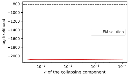
Take a mixture with \(K\ge2\) full-covariance components and \(N\) distinct data points. Fix the other components, set \(\bm\mu_1=\bm x_1\), \(\bm\Sigma_1=\sigma^2\bm I\), and let \(\sigma\to0\). The likelihood is \(\prod_n\sum_k\pi_k\N(\bm x_n\given\bm\mu_k,\bm\Sigma_k)\). The factor for \(n=1\) is at least \(\pi_1(2\pi\sigma^2)^{-D/2}\to\infty\). Each factor for \(n\ge2\) is at least \(\sum_{k\ge2}\pi_k\N(\bm x_n\given\bm\mu_k,\bm\Sigma_k)\), a fixed positive number independent of \(\sigma\), and the first component's contribution \(\pi_1(2\pi\sigma^2)^{-D/2}\exp(-\|\bm x_n-\bm x_1\|^2/2\sigma^2)\ge0\). Hence the likelihood is at least \(C\,\pi_1(2\pi\sigma^2)^{-D/2}\to\infty\) with \(C>0\). So the maximum likelihood estimate does not exist: the supremum is \(+\infty\), approached by a spike on a single data point (Figure 21.S4). The same happens for any component that can collapse onto \(\le D\) points. If one covariance matrix is shared by all components (tied, or one common spherical variance) the likelihood is bounded, because shrinking it makes every other point, at positive distance from all the means, extremely unlikely; a spherical covariance per component is not enough, since that component can still collapse alone.
Consequences. EM started at a reasonable point converges to a local maximum of the likelihood (the useful solution), but may be drawn into a degenerate one; implementations add a small floor \(\epsilon\bm I\) to every covariance (\(10^{-6}\) in the code), use a prior on \(\bm\Sigma_k\) (MAP-EM), or restart a collapsing component. The fits in Figure 21.14 are such local maxima. The unboundedness is another reason why model selection by the maximised likelihood is not meaningful and why a penalty or prior (BIC, WAIC) is used. \(\square\)
21.4.1.2 Unidentifiability and label switching
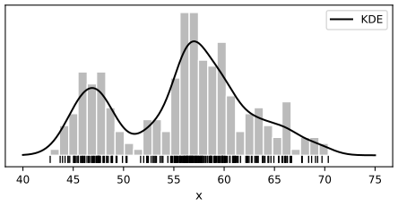
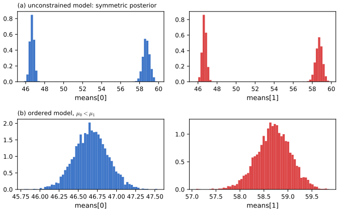
pp. 731–733 Permuting the component labels does not change the likelihood: the parameters are not identifiable, the label switching problem. It does not matter for the MLE or MAP, but it matters for posterior inference. Fitting two components to the one-dimensional data of Figure 21.15 by sampling gives, for each mean, a bimodal marginal posterior, one mode near 47 and one near 57 (Figure 21.16a), because either component can play either role. Imposing an ordering \(\mu_0<\mu_1\) by adding a penalty \[ \ell'(\bm\theta)=\log p(\mathcal D\given\bm\theta)+\log p(\bm\theta)+\phi(\bm\mu),\qquad\phi(\bm\mu)=\begin{cases}-\infty&\text{if }\mu_1<\mu_0\\0&\text{otherwise}\end{cases} \tag{21.25, 21.26} \] removes the symmetry (Figure 21.16b). A more general device is to transform the sampled parameters by an invertible map \(\bm\theta'=f(\bm\theta)\) and add the log-determinant of the Jacobian; the one-dimensional sort has determinant 1. The book notes that this does not scale to multi-dimensional centres, where there is no natural ordering.
Filling the gap 21.13: the symmetric posterior, and why the ordering constraint is legitimate pp. 731–733, (21.25), (21.26)
Derivation
Symmetry. Let \(\bm\theta=(\pi_k,\bm\mu_k,\bm\Sigma_k)_{k\le K}\) and for a permutation \(\rho\) of \(\{1,\dots,K\}\) let \(\bm\theta_\rho\) relabel the components. The mixture density \(\sum_k\pi_k\N(\bm x\given\bm\mu_k,\bm\Sigma_k)\) is unchanged by the relabelling, so \(p(\mathcal D\given\bm\theta_\rho)=p(\mathcal D\given\bm\theta)\). If the prior is exchangeable (the same prior for every component, as in the usual choices), \(p(\bm\theta_\rho)=p(\bm\theta)\), hence the posterior is invariant: \(p(\bm\theta_\rho\given\mathcal D)=p(\bm\theta\given\mathcal D)\). Consequently every marginal \(p(\bm\mu_k\given\mathcal D)\) is the same function of \(k\), and equals the average over the \(K!\) relabelled images of the posterior of the ordered parameters: with \(K=2\) and two well separated groups it has one mode at each group, as in Figure 21.16a. (A sampler may or may not hop between the \(K!\) modes; started in both orders, the pooled draws show both.) Quantities invariant under relabelling, such as the predictive density, the likelihood of a point or WAIC, are unaffected; those tied to a label, such as the mean of \(\bm\mu_1\), are meaningless without further structure.
The constraint. Let \(\Theta_<=\{\mu_1<\dots<\mu_K\}\) (one coordinate). The \(K!\) sets \(\rho(\Theta_<)\) tile the parameter space apart from the null set where two means coincide. By invariance, \(\int_\Theta p(\bm\theta\given\mathcal D)\,d\bm\theta=K!\int_{\Theta_<}p(\bm\theta\given\mathcal D)\,d\bm\theta=1\), so the posterior of the ordered model is \(K!\,p(\bm\theta\given\mathcal D)\) on \(\Theta_<\) and 0 elsewhere. Adding \(\phi\) with value \(-\infty\) outside \(\Theta_<\) to the log joint (21.25) sets the unnormalised density to zero outside \(\Theta_<\), and sampling from it gives exactly this renormalised restriction; the factor \(K!\) is a constant and plays no role. The sort transform \(\bm\theta\mapsto\text{sort}(\bm\theta)\) maps each \(\rho(\Theta_<)\) onto \(\Theta_<\) by a permutation of coordinates, which is linear with \(|\det|=1\), so the change-of-variables term is \(\log1=0\), as the book states. Careful reading: (21.26) as printed tests \(\mu_1<\mu_0\) while the text says the aim is \(\mu_1<\mu_2\); the indices must be consistent (here \(\mu_0<\mu_1\)).
Limits. The ordering of one coordinate fixes the labels only if the components are separated along that coordinate; with strongly overlapping means the ordered posterior can still be bimodal-looking, because the components with nearly equal means swap order, which is why the book recommends caution. In \(D>1\) there is no canonical order of the centres, so other devices (relabelling algorithms, or avoiding label-dependent summaries) are used. \(\square\)
21.4.1.3 Bayesian model selection
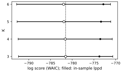
p. 733 Once identifiability is secured, the number of clusters can be chosen by Bayesian model comparison (Section 5.2.2). The book fits a GMM with \(K=3,\dots,6\) components to the data of Figure 21.15 by Hamiltonian Monte Carlo with an ordering transform on the means and compares them with a kernel density estimate (Figure 21.17); the models are compared by the widely applicable information criterion (WAIC), an approximation to the log marginal likelihood (Figure 21.18). I used a Gibbs sampler with conjugate priors in place of HMC (4 chains, 1000 draws each, means ordered); on the simulated data used here the four models fit equally well and WAIC does not separate them.
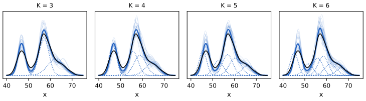
Filling the gap 21.14: WAIC, its penalty and what it estimates p. 733, [Wat10; Wat13; VGG17]
Derivation
Definition. With posterior draws \(\bm\theta^{(s)}\), \(s=1{:}S\), the log pointwise predictive density is \(\text{lppd}=\sum_{i=1}^N\log\big(\frac1S\sum_s p(y_i\given\bm\theta^{(s)})\big)\) (the in-sample log score of the posterior predictive) and the effective number of parameters is \(p_{\text{WAIC}}=\sum_i\operatorname{var}_s\big(\log p(y_i\given\bm\theta^{(s)})\big)\). Then \(\text{elpd}_{\text{WAIC}}=\text{lppd}-p_{\text{WAIC}}\) estimates the expected log score on new data; \(-2\,\text{elpd}_{\text{WAIC}}\) is the deviance scale, and the standard error of the estimate is \(\sqrt{N\operatorname{var}_i(e_i)}\) with \(e_i\) the pointwise terms. Larger elpd is better.
The penalty in a regular model. Let \(\ell_i(\bm\theta)=\log p(y_i\given\bm\theta)\) with gradient \(\bm g_i\) at the MLE. For a regular model with \(d\) parameters, the posterior is approximately \(\N(\hat{\bm\theta},(N\bm I_1)^{-1})\) with \(\bm I_1\) the per-observation Fisher information. To first order, \(\ell_i(\bm\theta)\approx\ell_i(\hat{\bm\theta})+\bm g_i^\T(\bm\theta-\hat{\bm\theta})\), so \(\operatorname{var}_s\ell_i\approx\bm g_i^\T(N\bm I_1)^{-1}\bm g_i\). Summing, \(p_{\text{WAIC}}\approx\operatorname{tr}\big((N\bm I_1)^{-1}\sum_i\bm g_i\bm g_i^\T\big)\approx\operatorname{tr}\big((N\bm I_1)^{-1}N\bm I_1\big)=d\), using \(\frac1N\sum_i\bm g_i\bm g_i^\T\to\bm I_1\) when the model is correctly specified. So \(p_{\text{WAIC}}\) estimates the number of parameters and WAIC is an AIC-like quantity that uses the whole posterior; in the code a one-parameter Gaussian-mean model gives \(p_{\text{WAIC}}=1.0\) to within 0.1. Watanabe (2010) shows that WAIC is asymptotically equivalent to leave-one-out cross-validation also for singular models such as mixtures, where \(p_{\text{WAIC}}\) is smaller than \(d\) (here 7.8 to 9.2 for \(3K-1=8\) to \(17\) parameters), which is the technical reason to prefer it to AIC or BIC for them (a cited result; the first-order argument above covers the regular case).
Label invariance. Each term \(\log\frac1S\sum_sp(y_i\given\bm\theta^{(s)})\) and each variance depend on the draws only through the likelihood of \(y_i\), which is invariant to relabelling (gap 21.13). So WAIC can be computed from unordered draws, and sorting the draws does not change it (checked in the code). \(\square\)
21.4.2 Mixtures of Bernoullis
pp. 733–734 For binary vectors \(\bm y\in\{0,1\}^D\) the component distribution is a product of Bernoullis, \[ p(\bm y\given z=k,\bm\theta)=\prod_{d=1}^D\operatorname{Ber}(y_d\given\mu_{dk})=\prod_{d=1}^D\mu_{dk}^{y_d}(1-\mu_{dk})^{1-y_d}, \tag{21.27} \] where \(\mu_{dk}\) is the probability that bit \(d\) is on in cluster \(k\). It can be fitted by EM, SGD or MCMC; Figure 3.13 clusters binarised MNIST digits this way.
See also: Bayesian and Probabilistic ML, Section 9.3.3 (mixtures of Bernoulli distributions) and its derivation in gap 9.12.
Filling the gap 21.15: EM for a mixture of Bernoullis p. 734, (21.27)
Derivation
E step. By Bayes' rule, with the product form (21.27), \(r_{nk}\propto\pi_k\prod_d\mu_{dk}^{y_{nd}}(1-\mu_{dk})^{1-y_{nd}}\), normalised over \(k\) (best computed with logs and log-sum-exp).
M step. Maximise the expected complete-data log-likelihood \(Q=\sum_n\sum_kr_{nk}\big[\log\pi_k+\sum_d\big(y_{nd}\log\mu_{dk}+(1-y_{nd})\log(1-\mu_{dk})\big)\big]\) subject to \(\sum_k\pi_k=1\). Differentiating in \(\mu_{dk}\): \(\sum_nr_{nk}\big(\frac{y_{nd}}{\mu_{dk}}-\frac{1-y_{nd}}{1-\mu_{dk}}\big)=0\), so \(\mu_{dk}=\sum_nr_{nk}y_{nd}/N_k\), \(N_k=\sum_nr_{nk}\) (the responsibility-weighted frequency of bit \(d\)); with a Lagrange multiplier for the weights, \(\pi_k=N_k/N\). The Hessian in \(\mu_{dk}\) is negative, so it is a maximum. Each EM sweep increases the log-likelihood (general EM argument, companion course Section 9.4). A cluster whose \(\mu_{dk}\) reaches 0 or 1 makes the likelihood of unseen patterns 0, so a Beta prior (add pseudo-counts) is used in practice. \(\square\)
21.5 Spectral clustering *
p. 734 Spectral clustering (Shi and Malik 2000; von Luxburg 2007) builds a similarity graph on the points, computes eigenvectors of a matrix of the graph, which give each point a feature vector, and clusters those with K-means.
See also: Elements of Statistical Learning, Section 14.5.3 (spectral clustering) with the demo spectral clustering on rings, and the Laplacian eigenmaps of Chapter 20 of the book (the same eigenvectors).
21.5.1 Normalized cuts
pp. 734–735 Build a weighted undirected graph with a node per data vector and edge weights \(w_{ij}=w_{ji}\ge0\) measuring similarity (typically only nearest neighbours are connected, to keep the graph sparse). The aim is a partition into disjoint node sets \(S_1,\dots,S_K\) of low cost. With \(W(A,B)=\sum_{i\in A,j\in B}w_{ij}\) and \(\bar S_k=V\setminus S_k\), the cut is \[ \operatorname{cut}(S_1,\dots,S_K)=\frac12\sum_{k=1}^KW(S_k,\bar S_k), \tag{21.28} \] the weight of the edges that are cut. Minimising it tends to split off a single node. The normalised cut divides by the size of each set measured by its volume \(\operatorname{vol}(A)=\sum_{i\in A}d_i\), with the weighted degree \(d_i=\sum_jw_{ij}\): \[ \operatorname{Ncut}(S_1,\dots,S_K)=\frac12\sum_{k=1}^K\frac{\operatorname{cut}(S_k,\bar S_k)}{\operatorname{vol}(S_k)}. \tag{21.29} \] Searching over indicator vectors \(\bm c_i\in\{0,1\}^N\) (\(c_{ik}=1\) iff point \(i\) is in cluster \(k\)) for the minimum is NP-hard (Wagner and Wagner 1993); the next sections give a continuous relaxation.
Filling the gap 21.17: Ncut as a trace, and its relaxation as an eigenproblem (Ky Fan) pp. 734–736, (21.29)
Derivation
Normalisation of the cut. In (21.29) \(\operatorname{cut}(S_k,\bar S_k)\) is the weight \(W(S_k,\bar S_k)\) of the edges leaving \(S_k\). I write \(\rho=\sum_kW(S_k,\bar S_k)/\operatorname{vol}(S_k)\); the book's Ncut is \(\rho/2\) (see the notes on the book for the factor 2, which does not move the minimiser).
A trace. Let \(\bm L=\bm D-\bm W\) and, for a partition, \(\bm h_k=\bm 1_{S_k}/\sqrt{\operatorname{vol}(S_k)}\), \(\bm H=[\bm h_1,\dots,\bm h_K]\in\R^{N\times K}\). Using \(\bm f^\T\bm L\bm f=\frac12\sum_{ij}w_{ij}(f_i-f_j)^2\) (gap 21.16), \(\bm h_k^\T\bm L\bm h_k=\frac1{\operatorname{vol}(S_k)}\cdot\frac12\sum_{ij}w_{ij}(\mathbb I_{i\in S_k}-\mathbb I_{j\in S_k})^2=\frac{W(S_k,\bar S_k)}{\operatorname{vol}(S_k)}\) (each cut edge is counted twice in the double sum, and halved). Hence \(\rho=\operatorname{tr}(\bm H^\T\bm L\bm H)\). The columns have disjoint supports, so \(\bm h_k^\T\bm D\bm h_l=0\) for \(k\ne l\), and \(\bm h_k^\T\bm D\bm h_k=\operatorname{vol}(S_k)/\operatorname{vol}(S_k)=1\): \(\bm H^\T\bm D\bm H=\bm I\). So \(\min\rho\) over partitions is the minimum of \(\operatorname{tr}(\bm H^\T\bm L\bm H)\) over matrices \(\bm H\) of this special form (a discrete set).
Relaxation. Drop the discreteness and keep \(\bm H^\T\bm D\bm H=\bm I\): \(\min_{\bm H}\operatorname{tr}(\bm H^\T\bm L\bm H)\). Substitute \(\bm T=\bm D^{1/2}\bm H\) (valid when all \(d_i>0\)): the constraint becomes \(\bm T^\T\bm T=\bm I\) and the objective \(\operatorname{tr}(\bm T^\T\bm L_{sym}\bm T)\), with \(\bm L_{sym}=\bm D^{-1/2}\bm L\bm D^{-1/2}\). Ky Fan: for symmetric \(\bm A\) with eigenpairs \((\lambda_i,\bm u_i)\), \(\lambda_1\le\dots\le\lambda_N\), and any \(\bm T\) with orthonormal columns \(\bm t_1,\dots,\bm t_K\): \(\operatorname{tr}(\bm T^\T\bm A\bm T)=\sum_i\lambda_ic_i\) with \(c_i=\sum_k(\bm u_i^\T\bm t_k)^2\). Each \(c_i\in[0,1]\) (Bessel: the squared norms of the projections of \(\bm u_i\) on an orthonormal set add up to at most \(\|\bm u_i\|^2=1\)) and \(\sum_ic_i=\sum_k\|\bm t_k\|^2=K\). The minimum of a linear function with weights in \([0,1]\) summing to \(K\) puts weight 1 on the \(K\) smallest eigenvalues, so \(\operatorname{tr}(\bm T^\T\bm A\bm T)\ge\lambda_1+\dots+\lambda_K\), with equality for \(\bm T=[\bm u_1,\dots,\bm u_K]\) (or any orthonormal basis of their span). So the relaxed minimum is the sum of the \(K\) smallest eigenvalues of \(\bm L_{sym}\), attained at \(\bm H=\bm D^{-1/2}[\bm u_1,\dots,\bm u_K]\): the eigenvectors of the random-walk Laplacian \(\bm L_{rw}\) (gap 21.18), solutions of the generalised problem \(\bm L\bm h=\lambda\bm D\bm h\).
Rounding. The relaxed \(\bm H\) is a real matrix, not of the discrete form. The \(i\)th row of \(\bm D^{-1/2}\bm U\) (or of the row-normalised \(\bm U\), as in the algorithm after (21.30)) is a \(K\)-dimensional feature vector for node \(i\); for an ideal graph with \(K\) components the rows take exactly \(K\) distinct values (gap 21.16), and K-means recovers the partition. As a bound: since the discrete \(\bm H\) are feasible, \(\sum_{i\le K}\lambda_i\le\rho_{\min}=2\,\operatorname{Ncut}_{\min}\). The relaxation lower-bounds the true optimum and is tight when the graph has exactly \(K\) components (the bound is then 0). \(\square\)
21.5.2 Eigenvectors of the graph Laplacian encode the clustering
pp. 735–736 The graph Laplacian is \(\bm L=\bm D-\bm W\) with \(\bm D=\operatorname{diag}(d_i)\), \(d_i=\sum_jw_{ij}\) (Section 20.4.9.2). Theorem 21.5.1: the eigenvectors of \(\bm L\) with eigenvalue 0 are spanned by the indicator vectors \(\bm 1_{S_1},\dots,\bm 1_{S_K}\) of the \(K\) connected components of the graph (proved in gap 21.16). The algorithm: take the eigenvectors of the \(K\) smallest eigenvalues of \(\bm L\) as the columns of \(\bm U\in\R^{N\times K}\), treat its rows \(\bm u_i\) as features (piecewise constant on components) and cluster them with K-means; these are the Laplacian-eigenmaps coordinates of Chapter 20. Real data have no exact block structure, but by perturbation theory (Ng et al. 2001) the eigenvectors of a slightly perturbed Laplacian stay close to the ideal indicators. In practice the Laplacian is normalised to account for the unequal degrees, \[ \bm L_{sym}=\bm D^{-1/2}\bm L\bm D^{-1/2}=\bm I-\bm D^{-1/2}\bm W\bm D^{-1/2}, \tag{21.30} \] whose zero eigenspace is spanned by \(\bm D^{1/2}\bm 1_{S_k}\). The algorithm of Ng, Jordan and Weiss: stack the \(K\) smallest eigenvectors of \(\bm L_{sym}\) into \(\bm U\), normalise each row to unit length, \(t_{ij}=u_{ij}/\sqrt{\sum_ku_{ik}^2}\), cluster the rows of \(\bm T\) by K-means, and give each original point the cluster of its row.
Filling the gap 21.16: the quadratic form, the null space (Theorem 21.5.1 for every \(K\)), the normalised variants and the spectrum pp. 735–736, (21.30), Theorem 21.5.1
Proof
Quadratic form. For \(\bm f\in\R^N\), \(\bm f^\T\bm L\bm f=\sum_id_if_i^2-\sum_{ij}w_{ij}f_if_j=\frac12\sum_{ij}w_{ij}(f_i^2+f_j^2)-\sum_{ij}w_{ij}f_if_j=\frac12\sum_{ij}w_{ij}(f_i-f_j)^2\), using \(\sum_id_if_i^2=\sum_{ij}w_{ij}f_i^2=\frac12\sum_{ij}w_{ij}(f_i^2+f_j^2)\) by symmetry of \(\bm W\). So \(\bm L\succeq0\) (the book's proof writes \(0=\sum_{ij}w_{ij}(f_i-f_j)^2\), omitting the factor \(\frac12\), which is immaterial there). The eigenvalues of \(\bm L_{sym}\) lie in \([0,2]\): \(\bm g^\T\bm L_{sym}\bm g=\frac12\sum w_{ij}(g_i/\sqrt{d_i}-g_j/\sqrt{d_j})^2\ge0\), and \(\le\sum w_{ij}(g_i^2/d_i+g_j^2/d_j)=2\|\bm g\|^2\) by \((a-b)^2\le2a^2+2b^2\).
Theorem 21.5.1. Let the graph have connected components \(S_1,\dots,S_K\) (nodes joined by a path of positive-weight edges). (i) Each \(\bm 1_{S_k}\) is in the null space. For \(i\in S_k\): \((\bm L\bm 1_{S_k})_i=d_i-\sum_jw_{ij}\mathbb I_{j\in S_k}=d_i-d_i=0\) (all neighbours of \(i\) are in \(S_k\)); for \(i\notin S_k\): \(0-\sum_jw_{ij}\mathbb I_{j\in S_k}=0\) (no edge to \(S_k\)). (ii) Nothing else is. If \(\bm L\bm f=0\) then \(\bm f^\T\bm L\bm f=0\), so \(w_{ij}(f_i-f_j)^2=0\) for every pair: \(f_i=f_j\) whenever \(w_{ij}>0\), hence \(f\) is constant along every path, i.e. constant on each component: \(\bm f=\sum_kc_k\bm 1_{S_k}\). The indicators of different components have disjoint supports and are linearly independent, so the null space has dimension exactly \(K\), the number of components. (The book proves \(K=1\) and says the case \(K>1\) is similar; the argument is the same componentwise, or one may order the nodes by component so that \(\bm L\) is block diagonal with one Laplacian block per component, each with a one-dimensional null space.) \(\square\)
Why K-means on the rows works. The \(K\) eigenvectors for eigenvalue 0 that an eigensolver returns are some orthonormal basis of \(\operatorname{span}\{\bm 1_{S_k}\}\), i.e. \(\bm U=\bm B\bm R\) where \(\bm B\) has columns \(\bm 1_{S_k}/\sqrt{|S_k|}\) and \(\bm R\) is an orthogonal \(K\times K\) matrix (unknown, because the eigensolver may rotate within the eigenspace). Row \(i\) of \(\bm U\) is then the row \(\bm r_k^\T/\sqrt{|S_k|}\) of \(\bm R\) for the component \(k\) of node \(i\): constant on components and different across components (the rows of \(\bm R\) are orthonormal). So K-means returns the components, whatever rotation was applied.
Normalised versions. \(\bm L_{sym}\bm D^{1/2}\bm 1_{S_k}=\bm D^{-1/2}\bm L\bm 1_{S_k}=0\), so \(\bm D^{1/2}\bm 1_{S_k}\) lie in its null space, and by the same argument they span it. Row \(i\) of the corresponding orthonormal \(\bm U\) is \(\sqrt{d_i}\cdot\bm r_k^\T/\sqrt{\operatorname{vol}(S_k)}\) for \(i\in S_k\): the scale factor \(\sqrt{d_i/\operatorname{vol}(S_k)}\) depends on the node but the direction \(\bm r_k\) only on the component; row normalisation divides by the norm and leaves exactly \(\bm r_k\), which is why the algorithm after (21.30) normalises the rows. For \(\bm L_{rw}=\bm D^{-1}\bm L\) the null space is \(\operatorname{span}\{\bm 1_{S_k}\}\) as for \(\bm L\); \(\bm L_{rw}=\bm D^{-1/2}\bm L_{sym}\bm D^{1/2}\) is similar to \(\bm L_{sym}\) (the same eigenvalues), and \(\bm L_{sym}\bm v=\lambda\bm v\) iff \(\bm L_{rw}(\bm D^{-1/2}\bm v)=\lambda(\bm D^{-1/2}\bm v)\), so eigenvectors of \(\bm L_{rw}\) are those of \(\bm L_{sym}\) rescaled by \(\bm D^{-1/2}\).
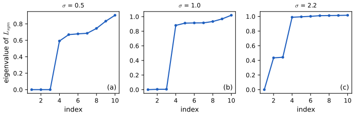
Perturbation. For a graph that is only nearly disconnected, the Davis-Kahan sin-theta theorem (cited) says that the subspace of the \(K\) smallest eigenvectors of a perturbed symmetric matrix \(\bm A+\bm E\) is at angle at most of order \(\|\bm E\|/\delta\) from that of \(\bm A\), where \(\delta\) is the gap between the \(K\)th and \((K+1)\)th eigenvalues of \(\bm A\); so the rows of \(\bm U\) cluster tightly when the between-cluster weights are small relative to the eigengap. Figure 21.S3 shows how the gap behaves as the width \(\sigma\) of the Gaussian affinity increases.
21.5.3 Example
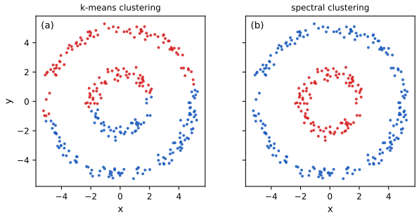
pp. 736–737 K-means is poor on data such as two concentric rings because it implicitly assumes spherical Gaussian clusters (Figure 21.19a). Spectral clustering with the dense Gaussian affinity \(W_{ij}=\exp(-\frac1{2\sigma^2}\|\bm x_i-\bm x_j\|_2^2)\), the first \(K=2\) eigenvectors of \(\bm L_{sym}\) and K-means on them recovers the rings (Figure 21.19b). The width matters: for the rings used here \(\sigma=0.5\) separates them exactly, while \(\sigma=1\) joins the rings too strongly (adjusted Rand index 0.07 in the code).
21.5.4 Connection with other methods
p. 737
21.5.4.1 Connection with kPCA
p. 737 Kernel PCA uses the largest eigenvectors of \(\bm W\), which are the smallest eigenvectors of \(\bm I-\bm W\); spectral clustering uses the smallest eigenvectors of \(\bm D-\bm W\) (or its normalisations). When all degrees are equal, \(d_i=d\), \(\bm L=d\bm I-\bm W\) and \(\bm L_{sym}=\bm I-\bm W/d\) have the same eigenvectors as \(\bm W\) in reverse order, so the two coincide; otherwise the degree normalisation makes spectral clustering behave better in practice (Bengio et al. 2004).
21.5.4.2 Connection with random walk analysis
p. 737 A third normalisation, \(\bm L_{rw}=\bm D^{-1}\bm L=\bm I-\bm D^{-1}\bm W\) (Shi and Malik 2000; Meila and Shi 2001), has the indicators \(\bm 1_{S_k}\) as zero-eigenvectors, so the \(K\) smallest eigenvectors can be clustered directly. The matrix \(\bm P=\bm D^{-1}\bm W=\bm I-\bm L_{rw}\) is stochastic with \(p_{ij}=w_{ij}/d_i\), the probability of stepping from \(i\) to \(j\) in a random walk. If the graph is connected and not bipartite the walk has a unique stationary distribution \(\pi_i=d_i/\operatorname{vol}(V)\), and for two clusters \[ \operatorname{Ncut}(S,\bar S)=p(S\given\bar S)+p(\bar S\given S), \tag{21.32} \] so a good cut is one such that the walk, in equilibrium, rarely moves between the two sets.
Filling the gap 21.18: the stationary distribution and (21.32) with its constant p. 737, (21.31), (21.32)
Proof
Stationary distribution. \(\bm P=\bm D^{-1}\bm W\) has non-negative entries and row sums \(\sum_jw_{ij}/d_i=1\). For \(\pi_i=d_i/\operatorname{vol}(V)\): \((\pi\bm P)_j=\sum_i\frac{d_i}{\operatorname{vol}}\frac{w_{ij}}{d_i}=\frac{d_j}{\operatorname{vol}}=\pi_j\), using the symmetry \(w_{ij}=w_{ji}\). The walk is moreover reversible: \(\pi_ip_{ij}=w_{ij}/\operatorname{vol}=\pi_jp_{ji}\). If the graph is connected the chain is irreducible, and if it is also non-bipartite (e.g. there are self-loops or odd cycles, which a Gaussian affinity with \(w_{ii}>0\) has) it is aperiodic, so by the Perron-Frobenius theorem (cited) the stationary distribution is unique and the chain converges to it.
The cut as a transition probability. Start the walk in equilibrium. The probability that it is in \(S\) and then steps to \(\bar S\) is \(\sum_{i\in S,j\in\bar S}\pi_ip_{ij}=\frac{W(S,\bar S)}{\operatorname{vol}(V)}\), and \(\pi(S)=\operatorname{vol}(S)/\operatorname{vol}(V)\). Therefore \(p(\bar S\given S)\equiv\Pr(X_1\in\bar S\given X_0\in S)=\frac{W(S,\bar S)}{\operatorname{vol}(S)}\) and \(p(S\given\bar S)=\frac{W(S,\bar S)}{\operatorname{vol}(\bar S)}\) (using \(W(S,\bar S)=W(\bar S,S)\)). The sum is \(\sum_kW(S_k,\bar S_k)/\operatorname{vol}(S_k)\) for \(K=2\), which is \(\rho=\operatorname{tr}(\bm H^\T\bm L\bm H)\) of gap 21.17.
The constant. With the definition (21.29), which carries a factor \(\frac12\), \(\operatorname{Ncut}(S,\bar S)=\frac12\big(p(\bar S\given S)+p(S\given\bar S)\big)\), half of the right side of (21.32). The identity (21.32) holds as printed for \(\sum_kW(S_k,\bar S_k)/\operatorname{vol}(S_k)\) (without the \(\frac12\)); I confirmed this numerically on a weighted graph. Since a constant factor does not change the minimiser, the algorithm is unaffected. Also, the eigenvalues of \(\bm P\) are \(1-\lambda\) for the eigenvalues \(\lambda\) of \(\bm L_{rw}\), so the smallest eigenvalues of \(\bm L_{rw}\) are the largest of \(\bm P\), the slowly decaying modes of the walk: the cluster structure is the metastable structure of the random walk (Meila and Shi 2001). \(\square\)
21.6 Biclustering *
p. 737 Biclustering (co-clustering) clusters the rows and the columns of a data matrix \(\bm X\in\R^{N_r\times N_c}\) together; it is used in bioinformatics (genes by conditions) and collaborative filtering (users by movies). The book presents a basic probabilistic model with one cluster id per row and one per column (Section 21.6.1) and an extension in which the row clustering depends on the group of columns (Section 21.6.2).
21.6.1 Basic biclustering
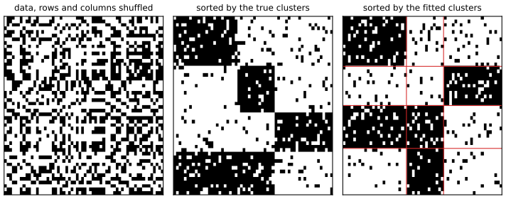
p. 738 Following Kemp et al. (2006), attach to each row \(i\) a latent \(u_i\in\{1,\dots,N_u\}\) and to each column \(j\) a latent \(v_j\in\{1,\dots,N_v\}\), with \[ p(\bm U)=\prod_{i=1}^{N_r}\operatorname{Unif}(u_i\given\{1,\dots,N_u\}),\quad p(\bm V)=\prod_{j=1}^{N_c}\operatorname{Unif}(v_j\given\{1,\dots,N_v\}),\quad p(\bm X\given\bm U,\bm V,\bm\theta)=\prod_{i=1}^{N_r}\prod_{j=1}^{N_c}p(X_{ij}\given\theta_{u_i,v_j}), \tag{21.33–21.35} \] where \(\theta_{a,b}\) are the parameters of the co-cluster of row cluster \(a\) and column cluster \(b\). (The book writes a categorical for \(\bm V\) in (21.34); with equal probabilities it is the same uniform distribution.) The book's example is a binary matrix of 50 animals by 85 features, in which the method finds 12 animal clusters and 33 feature clusters, using a Bayesian nonparametric prior for the numbers of clusters; for instance the cluster {antelope, horse, giraffe, zebra, deer} is characterised by the feature clusters {hooves, long neck, horns} and {walks, quadrupedal, ground} (Figure 21.20, from Kemp et al., not reproduced). Here the model with known numbers of clusters is fitted to a simulated matrix.
Filling the gap 21.19: the block likelihood, the collapsed form, and alternating maximisation p. 738, (21.33)–(21.35)
Derivation
Block log-likelihood. For binary data \(X_{ij}\sim\operatorname{Ber}(\theta_{u_iv_j})\), let for a block \((a,b)\) the number of cells be \(n_{ab}=|\{i:u_i=a\}||\{j:v_j=b\}|\) and the number of ones \(s_{ab}=\sum_{i:u_i=a}\sum_{j:v_j=b}X_{ij}\). Then \(\log p(\bm X\given\bm U,\bm V,\bm\theta)=\sum_{a,b}\big[s_{ab}\log\theta_{ab}+(n_{ab}-s_{ab})\log(1-\theta_{ab})\big]\), maximised over \(\theta_{ab}\) at \(\hat\theta_{ab}=s_{ab}/n_{ab}\) (the block frequency). With independent \(\operatorname{Beta}(\alpha,\beta)\) priors, \(\theta\) integrates out in closed form: \(p(\bm X\given\bm U,\bm V)=\prod_{a,b}B(\alpha+s_{ab},\beta+n_{ab}-s_{ab})/B(\alpha,\beta)\), the marginal likelihood used for collapsed sampling over \((\bm U,\bm V)\) or for comparing numbers of clusters.
Alternating maximisation. The code uses a simple hard-assignment scheme for known \(N_u,N_v\). Given \(\bm V\) and \(\bm\theta\), the log-likelihood is a sum over rows, and row \(i\) enters only through \(\sum_b\big[r_{ib}\log\theta_{u_ib}+(c_b-r_{ib})\log(1-\theta_{u_ib})\big]\), where \(r_{ib}=\sum_{j:v_j=b}X_{ij}\) and \(c_b=|\{j:v_j=b\}|\). Each \(u_i\) is therefore set independently to the best of the \(N_u\) values. Symmetrically for the columns given \(\bm U\). Re-estimating \(\hat{\bm\theta}\) in between is the exact block MLE. Each of the three steps does not decrease the log-likelihood, and there are finitely many assignments, so the iteration stops at a local maximum; several random starts are used. On the simulated matrix (50 by 60, four row and three column clusters) the fit recovers the row and column partitions exactly (adjusted Rand index 1 for both). The number of free parameters of the block model is \(N_uN_v+(N_r\log N_u+N_c\log N_v)/\log2\) bits for the assignments; this is what a model-selection criterion has to penalise. \(\square\)
21.6.2 Nested partition models (Crosscat)
pp. 738–740 In basic biclustering each object belongs to a single cluster. Intuitively an object can play several roles: animals can be grouped by anatomy (mammals, reptiles) or by behaviour (predators, prey). The nested partition (crosscat) model lets the row partition depend on the column group. With \(N_v\) column groups and, for each, an independent row clustering, \[ p(\bm U)=\prod_{i=1}^{N_r}\prod_{l=1}^{N_v}\operatorname{Unif}(u_{il}\given\{1,\dots,N_u\}),\quad p(\bm V)=\prod_{j=1}^{N_c}\operatorname{Unif}(v_j\given\{1,\dots,N_v\}), \tag{21.36, 21.37} \] \[ p(\bm Z\given\bm U,\bm V)=\prod_{i,j}\mathbb I\big(Z_{ij}=(u_{i,v_j},v_j)\big),\qquad p(\bm X\given\bm Z,\bm\theta)=\prod_{i,j}p(X_{ij}\given\theta_{Z_{ij}}), \tag{21.38, 21.39} \] with \(\theta_{k,l}\) the parameters of co-cluster \((k,l)\). In the book's \(6\times6\) example with \(N_u=2\), \(N_v=3\), column assignments \(\bm v=[1,1,2,3,3,3]\) and row partitions \(\bm u_{:,1}=[1,1,1,2,2,2]\), \(\bm u_{:,2}=[1,1,2,2,2,2]\), \(\bm u_{:,3}=[1,1,1,1,1,2]\), the rows are split differently in each column group (Figure 21.21b). The model was proposed independently as crosscat (Shafto et al. 2006; Mansinghka et al. 2016), multi-clust (Guan et al. 2010; Constantinopoulos et al. 2010) and nested partitioning (Rodriguez and Ghosh 2011), all with Dirichlet processes in place of fixed numbers of clusters. For the 22-animal data the MAP partition (Figure 21.22, from Shafto et al., not reproduced) finds a taxonomic column group that splits the animals into birds, reptiles and amphibians, mammals and invertebrates; a noise group; and an ecological group (dangerous, carnivore, lives in water) that splits them into prey, land predators, sea predators and air predators.
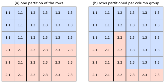
Filling the gap 21.20: the factorisation over column groups, the reduction to biclustering and the counts pp. 738–739, (21.36)–(21.39)
Derivation
Factorisation. Substituting the indicator (21.38) in (21.39), \(\log p(\bm X\given\bm U,\bm V,\bm\theta)=\sum_{l=1}^{N_v}\sum_{j:v_j=l}\sum_{i=1}^{N_r}\log p(X_{ij}\given\theta_{u_{il},l})\). The terms for column group \(l\) involve only \(\bm u_{:,l}\) and \(\theta_{\cdot,l}\): given the column partition, the model is a set of \(N_v\) independent clustering models (one mixture-like model for the rows per column group, each using the features of its group as "views"), with no coupling except through \(\bm V\). Hence the conditional posterior \(p(\bm U\given\bm V,\bm X)=\prod_lp(\bm u_{:,l}\given\bm X_{:,v=l})\) factorises over \(l\), and with Beta priors each factor is available in closed form as in gap 21.19, with block counts taken within the column group.
Reduction to biclustering. If all the row partitions are equal, \(\bm u_{:,l}=\bm u\) for every \(l\), then \(Z_{ij}=(u_i,v_j)\) and (21.35) is recovered. Conversely basic biclustering is the special case of crosscat in which the \(N_v\) row partitions are tied. Figure 21.21a is that case for \(\bm u=[1,1,1,2,2,2]\) and \(\bm v\) as above; Figure 21.21b relaxes it.
Counting. There are \(N_u^{N_r}\) assignments of rows for one partition, so basic biclustering ranges over \(N_u^{N_r}N_v^{N_c}\) configurations \((\bm U,\bm V)\) and crosscat over \(N_u^{N_rN_v}N_v^{N_c}\) (one row labelling per column group): for the \(6\times6\) example with \(N_u=2,N_v=3\) that is \(2^6\cdot3^6=46{,}656\) against \(2^{18}\cdot3^6=191{,}102{,}976\). The number of co-clusters is \(N_uN_v=6\) in both, but crosscat can place the same row in different row clusters in different column groups, e.g. row 3 is in cluster 1 for column groups 1 and 3 and in cluster 2 for group 2 (the cell labels 1.1, 2.2, 1.3 in the third row of Figure 21.21b). The labels \((k,l)\) written in the figure are exactly \(Z_{ij}\). \(\square\)
21.7 Exercises
The April 2025 draft of the book has no end-of-chapter exercises for Chapter 21. The four exercises below are my own, with complete solutions (hidden), and use the code of this chapter where a computation is asked for. They are numbered 21.1 to 21.4 for reference only.
Exercise 21.1 (agreement measures). Clusters 1, 2, 3 contain the classes \((A,B,C)\) in the counts \((5,1,0)\), \((1,4,1)\), \((2,0,3)\). (a) Compute the purity, the pair counts TP, FP, FN, TN, the Rand index and the adjusted Rand index. (b) Show that the Rand index of any partition against itself is 1 and that the adjusted Rand index of two independent random partitions is 0 in expectation, but the Rand index is not.
Solution
(a) Purity \((5+4+3)/17=12/17=0.706\). Cluster sizes 6, 6, 5: \(s_U=15+15+10=40\). Classes have sizes \(8,5,4\): \(s_V=28+10+6=44\). \(TP=\binom52+\binom42+\binom32+\binom22=10+6+3+1=20\) (also \(\binom12\)'s are 0). \(FP=40-20=20\), \(FN=44-20=24\), \(P=\binom{17}2=136\), \(TN=136-20-20-24=72\). Rand \(=92/136=0.676\). ARI \(=(20-40\cdot44/136)/(42-40\cdot44/136)=(20-12.94)/(42-12.94)=0.243\). (Code:
pair_counts,adjusted_rand.)(b) If \(U=V\), \(FP=FN=0\) and \(TP+TN=P\), so \(R=1\). For independent random partitions with the margins fixed, \(\E[TP]=s_Us_V/P\) (gap 21.1), so \(\E[R]=1+(2s_Us_V/P-s_U-s_V)/P=1-(s_U+s_V)/P+2s_Us_V/P^2\), which is not 0 (for equal fractions \(q=s_U/P=s_V/P\): \(1-2q+2q^2\ge\frac12\)); the ARI subtracts exactly this value so that \(\E[\text{ARI}]=0\). A simulation of 200 pairs of random four-cluster labellings of 300 points gave a mean ARI of \(0.000\pm0.01\), while the Rand index was about 0.63.
Exercise 21.2 (single link on five points). Use the points \(\bm x_1=(1,3)\), \(\bm x_2=(2.3,4.6)\), \(\bm x_3=(1,2)\), \(\bm x_4=(3,1)\), \(\bm x_5=(3,0)\) with city-block distance. (a) Run single link by hand and give the merge heights. (b) Verify that they are the sorted edge weights of a minimum spanning tree.
Solution
The distances are \(d_{13}=1\), \(d_{45}=1\), \(d_{12}=1.3+1.6=2.9\), \(d_{23}=1.3+2.6=3.9\), \(d_{34}=2+1=3\), \(d_{35}=2+2=4\), \(d_{14}=2+2=4\), \(d_{15}=5\), \(d_{24}=0.7+3.6=4.3\), \(d_{25}=0.7+4.6=5.3\). (a) Merge \(\{1,3\}\) at 1 and \(\{4,5\}\) at 1 (ties broken by index). Then the single-link distances are: \(d(\{1,3\},2)=\min(2.9,3.9)=2.9\); \(d(\{1,3\},\{4,5\})=\min(d_{14},d_{15},d_{34},d_{35})=3\); \(d(2,\{4,5\})=4.3\). The smallest is 2.9: point 2 joins \(\{1,3\}\). Finally \(d(\{1,2,3\},\{4,5\})=\min(3,\ 4.3,\ \dots)=3\). Heights \(1,1,2.9,3\). (b) Kruskal on the sorted edge list \((1,3):1\), \((4,5):1\), \((1,2):2.9\), \((3,4):3\) accepts these four edges (no cycles), a spanning tree of weight 7.9 and every other edge closes a cycle with heavier weight. The weights in order are exactly \(1,1,2.9,3\) (gap 21.2(c); Figure 21.2).
Exercise 21.3 (K-means as small-variance EM). For a GMM with \(\pi_k=1/K\) and \(\bm\Sigma_k=\sigma^2\bm I\), derive the E step, take \(\sigma^2\to0\), and show that the M step gives (21.14). Check numerically that the responsibilities approach the hard assignment of K-means.
Solution
Derivation as in gap 21.5: \(r_{nk}=\softmax_k(-\|\bm x_n-\bm\mu_k\|^2/2\sigma^2)\), \(1-r_{nk^*}\le(K-1)e^{-\delta/2\sigma^2}\), and the M step \(\bm\mu_k=\sum_nr_{nk}\bm x_n/\sum_nr_{nk}\) becomes the mean of the points whose nearest centre is \(\bm\mu_k\). Numerically (code, 400 blob points, \(K=3\), centres from K-means): the largest deviation of any responsibility from the hard assignment is about 0.49 for \(\sigma^2=1\), 0.32 for \(\sigma^2=0.05\) (points near cluster boundaries are still shared), and below \(10^{-100}\) for \(\sigma^2=10^{-4}\).
Exercise 21.4 (the Laplacian null space). A graph on nodes \(1,\dots,9\) has three cliques \(\{1,2,3\}\), \(\{4,5,6,7\}\), \(\{8,9\}\) with unit weights and no other edges. (a) Give the null space of \(\bm L\) and \(\bm L_{sym}\). (b) Show that adding one edge of weight \(\epsilon\) between two cliques leaves a single zero eigenvalue and a small second eigenvalue, and give a bound on it.
Solution
(a) By Theorem 21.5.1 the null space of \(\bm L\) is spanned by \(\bm 1_{\{1,2,3\}}\), \(\bm 1_{\{4,\dots,7\}}\), \(\bm 1_{\{8,9\}}\); for \(\bm L_{sym}\) by \(\bm D^{1/2}\) times these, with \(d_i=2,3,1\) in the three cliques. Eigenvalue 0 has multiplicity exactly 3 (code:
laplacians, three eigenvalues below \(10^{-10}\), and \(\bm L\bm 1_S=0\) to machine precision). (b) Connecting the cliques by an edge makes the graph connected, so the zero eigenvalue is simple. By the Courant-Fischer principle the second smallest eigenvalue is \(\lambda_2=\min_{\bm f\perp\bm 1}\bm f^\T\bm L\bm f/\|\bm f\|^2\). Take \(\bm f\) equal to \(a\) on the first two cliques and \(b\) on the third, with \(\bm f\perp\bm 1\) (so \(7a+2b=0\)). Then \(\bm f^\T\bm L\bm f=\epsilon(a-b)^2\) for the joining edge between the second and third cliques and \(\|\bm f\|^2=7a^2+2b^2\), with \(b=-3.5a\) (from \(7a+2b=0\)): \((a-b)^2=20.25a^2\) and \(7a^2+2b^2=31.5a^2\), so \(\lambda_2\le(20.25/31.5)\,\epsilon=0.643\,\epsilon\). The second eigenvalue is small, of order \(\epsilon\), and the corresponding eigenvector is nearly piecewise constant: the near-component structure that spectral clustering reads off.
Demonstrations
| Page | What it shows | In the notes |
|---|---|---|
| K-means: Lloyd steps, local minima and K-means++ | Step through the assignment and centre updates on 2000 points, choose random or K-means++ seeding, and compare the final distortion over 200 seeds. Presets: 1 a poor fixed start; 2 a K-means++ start; 3 random seeding; 4 200 seeds, K = 5; 5 200 seeds, K = 3. | 21.3.1, 21.3.4 |
| Distortion, silhouette and BIC | K from 2 to 8 on the blob data: the clusters, the silhouette diagram and the selection curves. Presets: 1 K = 3; 2 K = 5; 3 K = 2; 4 K = 8; 5 the elbow. | 21.3.7 |
| Hierarchical linkage | Single, complete and average link on blobs, moons, rings and gene-like profiles, with the dendrogram, the cut and the adjusted Rand index. Presets: 1 blobs; 2 moons, single; 3 moons, complete; 4 rings, single; 5 yeast-like profiles. | 21.2.1 |
The Python code that produces every figure of this page is code/ch21_clustering.py (see the code index). Companion demos: K-means and EM, mixture densities, K-means and hierarchical clustering, spectral clustering.
Notes on the book
Points where the book is imprecise or wrong
- (21.15), the matrix \(\bm Z\). The book writes \(\bm Z\in[0,1]^{N\times K}\); the identity \(J=\|\bm X-\bm Z\bm M^\T\|_F^2\) holds only for one-hot rows, \(\bm Z\in\{0,1\}^{N\times K}\) (gap 21.4(e)). Also (21.15) is the unnormalised sum while (21.17) divides by \(N\), so "the cost minimised by K-means" is the same up to the constant \(1/N\).
- Section 21.2.1, running time. "The other variants take \(O(N^3)\)" is the time of the naive implementation; for single, complete and average link (reducible linkages) the nearest-neighbour-chain algorithm needs \(O(N^2)\) time (gap 21.3).
- Section 21.3.7.1, monotone validation error. Fitting on a finite training set and evaluating on a validation set does not guarantee a monotone decrease in \(K\); it is the optimal training (or population) distortion that is non-increasing. With 25 training points the validation curve rose at some \(K\) in 14 of 40 random runs (gap 21.9). The conclusion (it cannot select \(K\)) stands.
- (21.21) and Figure 21.11b, sign of BIC. (21.21) is \(\log p-\frac{d}{2}\log N\), to be maximised, but the "U-shaped" curve of Figure 21.11b is the other sign convention, \(-2\log p+d\log N\) to be minimised (gap 21.11).
- Section 21.3.7.3, definition of the silhouette. The text takes the next closest cluster as the one with the nearest centroid; the standard definition (and common software) takes the cluster with the smallest mean distance. The two can differ (gap 21.10).
- (21.18). The numerator is written \(D_{t-1}(\bm x_n)\) while the text says the probability is proportional to the squared distance; with \(D_{t-1}\) defined as the squared distance in (21.19) it is consistent, and the proof of the guarantee needs the square (gap 21.7).
- (21.26), indices. The penalty tests \(\mu_1<\mu_0\) while the text says it imposes \(\mu_1<\mu_2\), and Figure 21.16 uses \(\mu_0<\mu_1\); the indices should agree (gap 21.13).
- (21.29) against (21.32), a factor 2. With \(\operatorname{cut}(S_k,\bar S_k)=W(S_k,\bar S_k)\) and the \(\frac12\) of (21.29), \(\operatorname{Ncut}(S,\bar S)=\frac12\big(p(S\given\bar S)+p(\bar S\given S)\big)\), not the sum as (21.32) states. (21.32) is right for \(\sum_kW(S_k,\bar S_k)/\operatorname{vol}(S_k)\), without the \(\frac12\). The minimiser is the same (gap 21.18).
- Proof of Theorem 21.5.1. The identity should read \(\bm f^\T\bm L\bm f=\frac12\sum_{ij}w_{ij}(f_i-f_j)^2\), and the case \(K>1\) is only indicated; it needs the argument componentwise (gap 21.16).
References
- Murphy, K. P. (2022). Probabilistic Machine Learning: An Introduction. MIT Press, Cambridge, MA. Chapter 21, pp. 715–740. probml.github.io/pml-book/book1.html.
- Arthur, D. and Vassilvitskii, S. (2007). k-means++: the advantages of careful seeding. Proceedings of the 18th ACM-SIAM Symposium on Discrete Algorithms, 1027–1035.
- Bengio, Y., Delalleau, O., Le Roux, N., Paiement, J.-F., Vincent, P. and Ouimet, M. (2004). Learning eigenfunctions links spectral embedding and kernel PCA. Neural Computation, 16(10), 2197–2219.
- Elkan, C. (2003). Using the triangle inequality to accelerate k-means. Proceedings of the 20th International Conference on Machine Learning.
- Figueiredo, M. A. T. and Jain, A. K. (2002). Unsupervised learning of finite mixture models. IEEE Transactions on Pattern Analysis and Machine Intelligence, 24(3), 381–396.
- Hubert, L. and Arabie, P. (1985). Comparing partitions. Journal of Classification, 2(1), 193–218.
- Kemp, C., Tenenbaum, J. B., Griffiths, T. L., Yamada, T. and Ueda, N. (2006). Learning systems of concepts with an infinite relational model. Proceedings of the 21st National Conference on Artificial Intelligence.
- Lloyd, S. P. (1982). Least squares quantization in PCM. IEEE Transactions on Information Theory, 28(2), 129–137.
- MacQueen, J. (1967). Some methods for classification and analysis of multivariate observations. Proceedings of the Fifth Berkeley Symposium, 1, 281–297.
- Meila, M. and Shi, J. (2001). A random walks view of spectral segmentation. Proceedings of the Eighth International Workshop on Artificial Intelligence and Statistics.
- Murtagh, F. (1983). A survey of recent advances in hierarchical clustering algorithms. The Computer Journal, 26(4), 354–359.
- Ng, A. Y., Jordan, M. I. and Weiss, Y. (2001). On spectral clustering: analysis and an algorithm. Advances in Neural Information Processing Systems, 14.
- Park, H.-S. and Jun, C.-H. (2009). A simple and fast algorithm for K-medoids clustering. Expert Systems with Applications, 36(2), 3336–3341.
- Sculley, D. (2010). Web-scale k-means clustering. Proceedings of the 19th International Conference on World Wide Web.
- Shafto, P., Kemp, C., Mansinghka, V., Gordon, M. and Tenenbaum, J. B. (2006). Learning cross-cutting systems of categories. Proceedings of the 28th Annual Conference of the Cognitive Science Society.
- Shi, J. and Malik, J. (2000). Normalized cuts and image segmentation. IEEE Transactions on Pattern Analysis and Machine Intelligence, 22(8), 888–905.
- von Luxburg, U. (2007). A tutorial on spectral clustering. Statistics and Computing, 17(4), 395–416.
- Wagner, D. and Wagner, F. (1993). Between min cut and graph bisection. Mathematical Foundations of Computer Science, 744–750.
- Watanabe, S. (2010). Asymptotic equivalence of Bayes cross validation and widely applicable information criterion in singular learning theory. Journal of Machine Learning Research, 11, 3571–3594.
The numerical statements in the text (the pair counts of Figure 21.1, the equality of the single-link tree with a minimum spanning tree, the descent of the distortion, the K-means++ sampling probabilities, the parameter counts, the Laplacian null space, and the Ncut identity) were confirmed numerically against independent library implementations.