Hypothesis Testing and p-values
A test turns data into a verdict, "reject the null hypothesis" or "retain it", and its quality is measured by two error probabilities: rejecting a true null (controlled by the size) and retaining a false one (one minus the power). This chapter builds the four workhorse tests (Wald, Pearson's chi-squared, permutation and likelihood ratio), the p-value, the corrections needed when thousands of tests are run at once, and, in the appendix, the one case where the best test is known exactly. The book states most of the theory without proof; these notes supply the proofs, check every number in the chapter, and show where the usual approximations fail in small samples.
Ch. 1 Probability Ch. 2 Random variables Ch. 3 Expectation Ch. 4 Inequalities Ch. 5 Convergence Ch. 6 Models and inference Ch. 7 Estimating the CDF Ch. 8 Bootstrap Ch. 9 Parametric inference Ch. 10 Hypothesis testing Ch. 11 Bayesian inference Ch. 12 Decision theory Ch. 13 Regression Ch. 14 Multivariate models Ch. 15 Independence Ch. 16 Causal inference Ch. 17 Directed graphs Ch. 18 Undirected graphs Ch. 19 Log-linear models Ch. 20 Curve estimation Ch. 21 Orthogonal functions Ch. 22 Classification Ch. 23 Stochastic processes Ch. 24 Simulation
How to read these notes
They follow the book. Sections carry the book's numbers (10.1, 10.2, ...) and every displayed equation that appears in the book carries the book's own equation number, e.g. \((10.6)\). Numbered items keep the book's numbers (Definition 10.1, Theorem 10.6, Example 10.18); items the book states without a number are lettered (Definition 10.A, Algorithm 10.A, ...). Equations without a number are steps that the book skips.
Filling the gaps. Wherever the book says "it can be shown", leaves a proof as an exercise or quotes a result from the literature, an orange Filling the gap box gives the full argument. Proofs and derivations start hidden: open one with its bar, or use the button below.
Figures and demonstrations. Figures 10.1, 10.4, 10.5 and 10.6 of the book are recomputed by the Python code; Figures 10.2 and 10.3 are hand-drawn schematics and are described in words. Seven supplementary figures (10.S1 to 10.S7) illustrate the gaps. The ▶ Demo boxes open an interactive demonstration already set to the case being discussed.
Main reference
L. Wasserman, All of Statistics: A Concise Course in Statistical Inference, Springer (2004), Chapter 10, pages 149–173 (book website: www.stat.cmu.edu/~larry/all-of-statistics). Section, equation, example and exercise numbers below refer to this book. Further reading is listed in the references.
The explanations, derivations, figures and code are my own; equations are cited by their numbers in the book.
Companion courses
Hypothesis testing is taught, at other levels and in other words, in four companion courses on this site. The overlapping material is:
- First-year notes, Estimation and hypothesis testing (advanced): the logic of tests (Section 4), p-values control the type I error (Theorem 4.1, our Theorem 10.14), tests and intervals are two views of one object (Theorem 4.2, our Theorem 10.10), the t-test and power (Section 5), the Neyman–Pearson lemma (Theorem 6.1, our Theorem 10.30), two samples (Section 8) and two proportions (Section 9). Its demos: a hypothesis test on trial, power and sample size, tests and intervals.
- Statistical Methods for Modern Biology, Chapter 6 (testing): uniform p-values (Result 6.1), Neyman–Pearson for a coin (Result 6.2), the t distribution (Result 6.3), permutation tests (Result 6.4), Bonferroni (Result 6.5) and the false discovery rate proved in full (Result 6.6); and Chapter 2, Pearson's theorem (Result 2.4, proof in Filling the gap 2.6).
- Applied Statistical Learning in R and Python, Chapter 13 (multiple testing): errors and power (Definition 13.2), the family-wise error rate and Bonferroni (Result 13.3), Benjamini–Hochberg (Result 13.5), permutation p-values (Result 13.6).
- Statistical Learning: Theory and Methods, Chapter 18: feature assessment and multiple testing (Section 18.7), Bonferroni (Result 18.11) and Benjamini–Hochberg (Result 18.12) for gene expression data.
Where a proof there is complete, these notes give the statement and a short argument and link to it. New here: the exact size of the Wald test in discrete models (Filling the gap 10.2), the power formula and local alternatives (10.3), the p-value as a diagnostic test (10.8), the permutation p-value and its ties (10.11), Wilks' theorem (10.12), the Chernoff–Lehmann bound (10.15) and the small-sample size of chi-squared-calibrated tests (Exercises 10.13 to 10.15). Within this course, Chapter 6 introduced the vocabulary (Section 6.3.3).
The chapter at a glance
- Introduction. A test is a rejection region; its power function \(\beta(\th)\) gives the rejection probability, its size is the largest rejection probability under the null (Definition 10.1); Example 10.2 computes both for a Normal mean (Filling the gap 10.1).
- 10.1 The Wald test standardises an asymptotically Normal estimator; its size tends to \(\alpha\) (Theorem 10.4), its power is (10.6) (Theorem 10.6), and it rejects exactly when the confidence interval misses \(\th_0\) (Theorem 10.10).
- 10.2 The p-value is the smallest level at which the test rejects (Definition 10.11), a tail probability (Theorem 10.12), uniform under a continuous null (Theorem 10.14), and not the probability that the null is true (10.8).
- 10.3–10.4 The \(\chi^2\) family (10.9) and Pearson's test for multinomial data (Theorem 10.17, 10.10), with Mendel's peas.
- 10.5 The permutation test is exact when the p-value counts ties (10.11).
- 10.6 The likelihood ratio statistic is asymptotically \(\chi^2\) with as many degrees of freedom as constraints (Theorem 10.22, 10.12).
- 10.7 Bonferroni controls the chance of any false rejection (Theorem 10.24), Benjamini–Hochberg the expected proportion of false rejections (Theorem 10.26, 10.14).
- 10.8 Goodness-of-fit with estimated parameters loses one degree of freedom per parameter (Theorem 10.29, 10.15).
- 10.10 The likelihood ratio test is most powerful for simple hypotheses (Theorem 10.30, 10.16); the t-test is exact for Normal data (10.17).
Notation. Data \(X^n=(X_1,\dots,X_n)\) with observed value \(x^n\); \(\P_\th\) and \(\E_\th\) are computed when the parameter is \(\th\). \(\Phi\) is the standard Normal cdf, \(Z\) a \(N(0,1)\) variable and \(z_\alpha=\Phi^{-1}(1-\alpha)\) its upper \(\alpha\) quantile. \(\chisq{k}\) is the chi-squared distribution with \(k\) degrees of freedom and \(\chisq{k,\alpha}\) its upper \(\alpha\) quantile. \(\convp\) and \(\convd\) denote convergence in probability and in distribution (Chapter 5 of the book).
Prerequisites. Chapters 5, 6 and 9 of the book: the central limit theorem, Slutsky's theorem and the delta method (Theorem 5.5, 5.8, 5.13), the vocabulary of inference (Chapter 6), and maximum likelihood with its asymptotic normality (Chapter 9). See the course home.
The language of testing
pp. 149–151 The book opens with a randomised experiment: rats are split at random into an asbestos-exposed group and a control group, and we ask whether the disease rates differ. The null hypothesis says they do not; the alternative says they do. Formally the parameter space is split into two disjoint pieces and we test
\[ H_0:\ \th\in\Theta_0\qquad\text{versus}\qquad H_1:\ \th\in\Theta_1. \tag{10.1} \]A test is a set \(R\) of possible data values, the rejection region: reject \(H_0\) when \(X\in R\), retain it otherwise. Usually
\[ R=\big\{x:\ T(x)>c\big\} \tag{10.2} \]for a test statistic \(T\) and a critical value \(c\). Two errors are possible. Rejecting a true null is a type I error; retaining a false null is a type II error (the book's Table 10.1). The courtroom analogy fits: the defendant (the null) is presumed innocent, and the verdict "guilty" needs strong evidence. "Retain" is not "accept": a test that retains \(H_0\) has failed to find evidence against it, which is not evidence for it.
| retain \(H_0\) | reject \(H_0\) | |
|---|---|---|
| \(H_0\) true | correct | type I error |
| \(H_1\) true | type II error | correct |
The book's first warning deserves repeating: a test answers a yes-or-no question about a well-defined hypothesis. When the real question is "how big is the effect?", an estimate with a confidence interval answers it better (see Theorem 10.10 and the warning after it).
Definition 10.1 (power function, size, level) p. 150, (10.3)–(10.4)
The power function of a test with rejection region \(R\) is
\[ \beta(\th)=\P_\th(X\in R). \tag{10.3} \]The size of the test is the largest probability of a type I error,
\[ \text{size}=\sup_{\th\in\Theta_0}\beta(\th), \tag{10.4} \]and the test has level \(\alpha\) if its size is at most \(\alpha\). A hypothesis \(\th=\th_0\) is simple; one such as \(\th>\th_0\) is composite. Testing \(\th=\th_0\) against \(\th\ne\th_0\) is two-sided; testing \(\th\le\th_0\) against \(\th>\th_0\) (or the reverse) is one-sided.
So \(\beta\) on \(\Theta_0\) is the type I error probability and \(1-\beta\) on \(\Theta_1\) is the type II error probability: one function carries both errors. A good test has \(\beta\) small on \(\Theta_0\) and large on \(\Theta_1\); since \(\beta\) is usually continuous, it cannot jump from \(\alpha\) to 1 at the boundary, and near the boundary the power is necessarily close to the size.
See also: the first-year notes, the logic of tests; Statistical Methods for Modern Biology, Section 6.4 (types of error); Applied Statistical Learning, Definition 13.2.
Example 10.2 (a one-sided test of a Normal mean) p. 151
Let \(X_1,\dots,X_n\sim N(\mu,\sigma^2)\) with \(\sigma\) known, and test \(H_0:\mu\le0\) against \(H_1:\mu>0\) by rejecting when \(\overline X_n>c\). Standardising,
\[ \beta(\mu)=\P_\mu\Big(\frac{\sqrt n(\overline X_n-\mu)}{\sigma}>\frac{\sqrt n(c-\mu)}{\sigma}\Big)=1-\Phi\Big(\frac{\sqrt n(c-\mu)}{\sigma}\Big). \]This is increasing in \(\mu\), so the size is \(\beta(0)=1-\Phi(\sqrt n c/\sigma)\). Setting it equal to \(\alpha\) gives \(c=\sigma z_\alpha/\sqrt n\): reject when \(\sqrt n\,\overline X_n/\sigma>z_\alpha\). With \(n=10\), \(\sigma=1\) and \(\alpha=0.05\), \(c=0.520\).
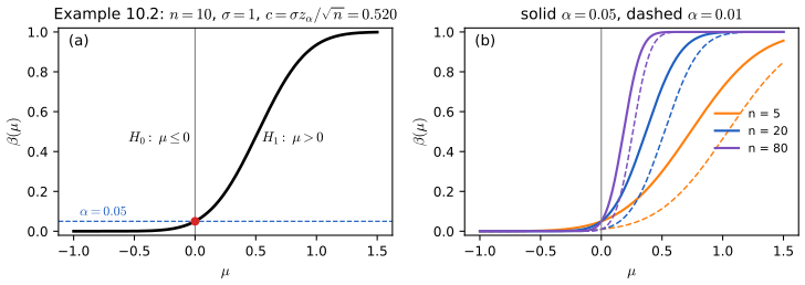
fig_10_1. Download: PDF · SVGFilling the gap 10.1: why the size is attained at the boundary, and why this test is the best one pp. 151–152
Three facts are used without comment. (a) \(\beta\) is strictly increasing and continuous, so \(\sup_{\mu\le0}\beta(\mu)=\beta(0)\) and the composite null is "as hard as" its boundary point. (b) Hence the test has level \(\alpha\) for the whole composite null although \(c\) was chosen from one point. (c) The book remarks after the figure that most powerful tests are hard to find; for this example one exists: among all tests with level \(\alpha\) for \(H_0:\mu\le0\), this one has the largest power at every \(\mu>0\) (it is uniformly most powerful).
Proof
(a) \(\beta(\mu)=1-\Phi(\sqrt n(c-\mu)/\sigma)\) and \(\Phi\) is continuous and strictly increasing, so \(\beta\) is continuous and strictly increasing in \(\mu\); the supremum over \((-\infty,0]\) is the value at 0. (b) For \(\mu\le0\), \(\beta(\mu)\le\beta(0)=\alpha\). (c) Fix \(\mu_1>0\) and any test \(\phi\) (a function of the data with values in \([0,1]\), the probability of rejecting) with \(\sup_{\mu\le0}\E_\mu\phi\le\alpha\); in particular \(\E_0\phi\le\alpha\). The likelihood ratio of \(N(\mu_1,\sigma^2)\) to \(N(0,\sigma^2)\) samples is \[ \exp\{n\mu_1\overline x/\sigma^2-n\mu_1^2/(2\sigma^2)\}, \] increasing in \(\overline x\), so our test is the Neyman–Pearson test of \(\mu=0\) against \(\mu=\mu_1\). By Theorem 10.30 (proved in Filling the gap 10.16), no test with \(\E_0\phi\le\alpha\) has more power at \(\mu_1\). The test does not depend on \(\mu_1\), so it is most powerful at every \(\mu_1>0\) simultaneously. ∎
The argument works whenever the likelihood ratio is monotone in one statistic (a monotone likelihood ratio family: Normal, Binomial, Poisson, Exponential and the other one-parameter exponential families). For two-sided alternatives no uniformly most powerful test exists: the most powerful test against \(\mu_1>0\) rejects for large \(\overline x\), against \(\mu_1<0\) for small \(\overline x\), and no single test does both.
10.1 The Wald Test
pp. 152–153 The first general-purpose test needs only an estimator that is approximately Normal, which by Chapter 9 the MLE is in regular models. Abraham Wald (1902–1950) introduced it.
Definition 10.3 (the Wald test) p. 153, (10.5)
Let \(\th\) be a scalar parameter, \(\hth\) an estimator and \(\hse\) its estimated standard error, and suppose \((\hth-\th_0)/\hse\convd N(0,1)\) when \(\th=\th_0\). To test \(H_0:\th=\th_0\) against \(H_1:\th\ne\th_0\), the size \(\alpha\) Wald test rejects when \(|W|>z_{\alpha/2}\), where
\[ W=\frac{\hth-\th_0}{\hse}. \tag{10.5} \]Theorem 10.4 (the Wald test has asymptotic size \(\alpha\)) p. 153
Under the assumption of Definition 10.3, \(\P_{\th_0}(|W|>z_{\alpha/2})\to\alpha\) as \(n\to\infty\).
Proof
Under \(\th_0\), \(W\convd Z\sim N(0,1)\). The set \(\{w:|w|>z_{\alpha/2}\}\) has boundary \(\{\pm z_{\alpha/2}\}\), which has probability 0 under the continuous law of \(Z\); by the portmanteau characterisation of convergence in distribution (or directly, because \(\P(|W|>z)=1-F_W(z)+F_W(-z^-)\) and \(F_W\to\Phi\) at the continuity points \(\pm z\)),
\[ \P_{\th_0}(|W|>z_{\alpha/2})\to\P(|Z|>z_{\alpha/2})=2\big(1-\Phi(z_{\alpha/2})\big)=\alpha. \]Note what is and is not claimed: the size converges to \(\alpha\) for each fixed \(\th_0\); nothing is said about how fast, and in discrete models the exact size can be far from \(\alpha\) for moderate \(n\) (next box). ∎
p. 153 Remark 10.5. One may standardise instead by \(\se_0\), the standard error computed at \(\th=\th_0\) (for a proportion, \(\sqrt{p_0(1-p_0)/n}\) rather than \(\sqrt{\hat p(1-\hat p)/n}\)). The book says both versions are valid.
Filling the gap 10.2: why both standard errors are valid, and how different they are in small samples p. 153, Remark 10.5
(a) If \((\hth-\th_0)/\se\convd N(0,1)\) under \(\th_0\) and \(\hse/\se\convp1\), then both \((\hth-\th_0)/\hse\) and \((\hth-\th_0)/\se_0\) converge to \(N(0,1)\) under \(\th_0\), so both Wald tests have asymptotic size \(\alpha\). (b) In discrete models the exact size of either version, \(\sum_s\P_{\th_0}(S=s)\,\I\{|W(s)|>z_{\alpha/2}\}\), is a step function of \(n\) that oscillates around \(\alpha\) and can be far from it: for the Bernoulli model with \(p_0=0.5\) it is 0.219 at \(n=6\), 0.041 at \(n=20\) and 0.081 at \(n=40\); with \(p_0=0.1\) and \(n=30\) it is 0.191 with the estimated standard error and 0.026 with \(\se_0\).
Proof and numbers
(a) Under \(\th_0\), \(\se_0\) is the true standard error, so the second statistic converges by assumption. For the first, \[ (\hth-\th_0)/\hse=\{(\hth-\th_0)/\se\}\cdot(\se/\hse), \] a product of a sequence converging in distribution to \(N(0,1)\) and one converging in probability to 1; Slutsky's theorem (Theorem 5.5) gives the limit \(N(0,1)\). For a proportion, \[ \hse/\se_0=\sqrt{\hat p(1-\hat p)}/\sqrt{p_0(1-p_0)}\convp1 \] by the law of large numbers and the continuity of \(p\mapsto\sqrt{p(1-p)}\) at \(p_0\in(0,1)\).
(b) Let \(S=\sum_iX_i\sim\Bin(n,p_0)\). The Wald statistic is a function \(W(S)\), so the rejection event is a union of atoms \(\{S=s\}\) and the exact size is the finite sum above, computed by wald_exact_power. As \(n\) grows, the lattice of values \(s/n\) shifts relative to the cut-offs \(p_0\pm z_{\alpha/2}\hse\), and atoms of size about \(1/\sqrt n\) enter and leave the rejection region: hence the saw-tooth in Figure 10.S1(c), with amplitude of order \(n^{-1/2}\). With \(p_0=0.1\), \(n=30\) and the estimated standard error, \(S=0\) gives \(\hse=0\) (rejected by convention, as the estimate differs from \(p_0\)) and \(S=1\) gives \[ W=(1/30-0.1)/\sqrt{(1/30)(29/30)/30}=-2.03, \] also rejected; \(\P(S\le1)=0.9^{30}+30(0.1)(0.9^{29})=0.184\), most of the size 0.191. With \(\se_0=\sqrt{0.1\cdot0.9/30}=0.0548\), \(S=1\) gives \(W=-1.22\) and is retained. Neither version is uniformly better: the estimated standard error is too small when \(\hat p\) is near 0 or 1, the null one is fixed, and the comparison reverses for other \((n,p_0)\). ∎
pp. 153–154 What happens when the null is false?
Theorem 10.6 (power of the Wald test) p. 153, (10.6)
If the true value is \(\th_\star\ne\th_0\), the power of the Wald test is approximately
\[ \beta(\th_\star)\approx1-\Phi\Big(\frac{\th_0-\th_\star}{\hse}+z_{\alpha/2}\Big)+\Phi\Big(\frac{\th_0-\th_\star}{\hse}-z_{\alpha/2}\Big). \tag{10.6} \]The power is large when \(\th_\star\) is far from \(\th_0\) and when \(n\) is large (\(\hse\to0\)).
Filling the gap 10.3: proof of (10.6) (Exercise 10.1), consistency of the test (Exercise 10.9), and local alternatives pp. 153–154
Assume that under \(\th_\star\), \((\hth-\th_\star)/\se\convd N(0,1)\) and \(\hse/\se\convp1\), where \(\se=\se(\th_\star)\to0\). Then (a) the power satisfies \(\beta(\th_\star)-g(\th_\star)\to0\), where \(g\) is the right side of (10.6) with \(\se\) in place of \(\hse\); for a Normal mean with known \(\sigma\), (10.6) is exact. (b) For fixed \(\th_\star\ne\th_0\), \(\beta(\th_\star)\to1\): the Wald test is consistent. (c) For local alternatives \(\th_n=\th_0+h/\sqrt n\) with \(\sqrt n\,\se\to\tau\), the power tends to \[ 1-\Phi(z_{\alpha/2}-h/\tau)+\Phi(-z_{\alpha/2}-h/\tau), \] strictly between \(\alpha\) and 1. (d) Hence the sample size for power \(1-\gamma\) at distance \(\Delta=|\th_\star-\th_0|\) is about \(n=\tau^2(z_{\alpha/2}+z_\gamma)^2/\Delta^2\).
Proof
(a) Write \[ W=(\hth-\th_\star)/\hse+(\th_\star-\th_0)/\hse=A_n+B_n. \] The approximation of the book treats \(A_n\) as \(Z\) and \(B_n\) as the constant \(\delta_n=(\th_\star-\th_0)/\se\). Then
\[ \P(W>z_{\alpha/2})\approx\P(Z>z_{\alpha/2}-\delta_n)=1-\Phi(z_{\alpha/2}-\delta_n),\qquad \P(W<-z_{\alpha/2})\approx\Phi(-z_{\alpha/2}-\delta_n), \]and since \(-\delta_n=(\th_0-\th_\star)/\se\) the sum is (10.6). To make "\(\approx\)" precise: if \(\delta_n\) stays bounded, \(A_n\convd Z\) and \(B_n-\delta_n\convp0\) (because \(\se/\hse\convp1\)) give, along subsequences where \(\delta_n\) converges, convergence of both probabilities by Slutsky's theorem and the continuity of \(\Phi\), so \(\beta-g\to0\). If \(|\delta_n|\to\infty\), both \(\beta\) and \(g\) tend to 1 (part b). For \(X_i\sim N(\th,\sigma^2)\) with \(\sigma\) known, \(\hth=\overline X_n\) and \(\se=\sigma/\sqrt n\) is not estimated: \(A_n\) is exactly \(N(0,1)\), \(B_n=\delta_n\) exactly, and (10.6) is an identity.
(b) With \(\th_\star>\th_0\) say, \(\delta_n=(\th_\star-\th_0)/\se\to\infty\). If \(A_n>-\delta_n/2\) and \(B_n>\delta_n/2+z\) then \(W>z\), so
\[ \P(W>z)\ge1-\P(A_n\le-\delta_n/2)-\P(B_n\le\delta_n/2+z)\to1, \]because \(A_n\) is tight (it converges in distribution) and \[ B_n-\delta_n/2-z=\delta_n(B_n/\delta_n-1/2)-z\to\infty \] in probability, as \(B_n/\delta_n=\se/\hse\convp1\). This is Exercise 10.9, where \(\se=\{nI(\th)\}^{-1/2}\) is the Fisher-information standard error of the MLE.
(c) Now \(\delta_n=h/(\sqrt n\se)\to h/\tau\) and the limit follows from (a). This is the honest meaning of (10.6): against alternatives at distance of order \(n^{-1/2}\), power stays bounded away from 1, and (10.6) is its limit.
(d) Ignoring the smaller of the two terms, power \(1-\gamma\) needs \(z_{\alpha/2}-\Delta\sqrt n/\tau=-z_\gamma\). ∎
For a Normal mean with \(\sigma=1\), \(n=25\), \(\alpha=0.05\) and \(\th_\star=0.4\): \(\delta=2\) and the power is \(1-\Phi(-0.04)+\Phi(-3.96)=0.516\). Power 0.8 at the same distance needs \(n=(1.96+0.84)^2/0.4^2=49.1\), so 50 observations. For a Bernoulli parameter the approximation can be poor at moderate \(n\): with \(p_0=0.5\), \(n=20\) and \(p_\star=0.7\), (10.6) gives 0.497 while the exact power is 0.416 (Figure 10.S1(b)).
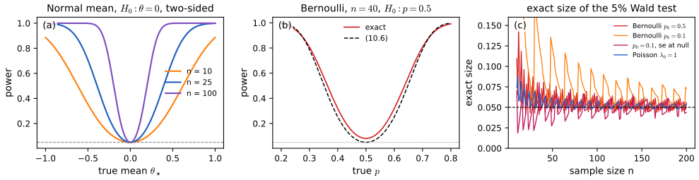
fig_10_s1. Download: PDF · SVGSee also: the first-year notes, power and sample size and the power demo; Statistical Methods for Modern Biology, power and sample size for a coin.
Example 10.7 (comparing two prediction algorithms) pp. 154–155
Algorithm 1 makes \(X\sim\Bin(m,p_1)\) errors on one test set and algorithm 2 makes \(Y\sim\Bin(n,p_2)\) errors on an independent one. For \(\delta=p_1-p_2\), the MLE is \(\hat\delta=\hat p_1-\hat p_2\) with \[ \hse^2=\hat p_1(1-\hat p_1)/m+\hat p_2(1-\hat p_2)/n, \] and the Wald test rejects \(\delta=0\) when \(|\hat\delta/\hse|>z_{\alpha/2}\). If both algorithms are run on the same \(n\) cases, the samples are dependent; with \(X_i,Y_i\in\{0,1\}\) the indicators of a correct prediction on case \(i\) and \(D_i=X_i-Y_i\), use \(\hat\delta=\overline D\), \(\hse=S/\sqrt n\) with \(S^2=n^{-1}\sum_i(D_i-\overline D)^2\): the paired comparison.
Filling the gap 10.4: why the paired standard error is the right one, and what pairing buys pp. 154–155
Assume the \(n\) test cases are iid draws, so the pairs \((X_i,Y_i)\) are iid. Then (a) \(\sqrt n(\overline D-\delta)/S\convd N(0,1)\), so the paired Wald test has asymptotic size \(\alpha\); (b) \(\V(D_i)=\V(X_i)+\V(Y_i)-2\Cov(X_i,Y_i)\), so the unpaired formula, which ignores the covariance, is wrong for paired data; (c) when the two algorithms tend to succeed on the same cases (\(\Cov>0\), the usual situation) pairing reduces the variance and raises the power.
Proof
(a) The \(D_i\) are iid with mean \(\delta=\P(X_i=1)-\P(Y_i=1)\) and finite variance \(\sigma_D^2\) (they are bounded). The central limit theorem gives \[ \sqrt n(\overline D-\delta)/\sigma_D\convd N(0,1); \] the law of large numbers gives \(S^2\convp\sigma_D^2\); Slutsky's theorem combines them, provided \(\sigma_D>0\) (if the two algorithms always agree, \(D_i\equiv0\) and there is nothing to test). (b) Expand the variance of a difference. (c) The variance of \(\overline D\) is \(\{\V(X)+\V(Y)-2\Cov(X,Y)\}/n\), against \(\{\V(X)+\V(Y)\}/n\) for two independent test sets of the same size; a positive covariance shrinks the standard error, which by Filling the gap 10.3(d) is equivalent to a larger sample. Only the discordant cases (\(D_i=\pm1\)) carry information about \(\delta\), which is why the exact version of this test is McNemar's test on the discordant pairs. ∎
See also: the first-year notes, why pairing helps, and the two-sample demo.
p. 155 Example 10.8 (comparing two means). For independent samples \(X_1,\dots,X_m\) and \(Y_1,\dots,Y_n\) with means \(\mu_1,\mu_2\), the plug-in estimate of \(\delta=\mu_1-\mu_2\) is \(\overline X-\overline Y\) with \(\hse=\sqrt{s_1^2/m+s_2^2/n}\), and the Wald statistic is \(W=(\overline X-\overline Y)/\hse\). Example 10.9 (comparing two medians) replaces the means by sample medians \(\hat\nu_1-\hat\nu_2\) and obtains \(\hse\) from the bootstrap (Chapter 8); the Wald test is valid if the difference of sample medians is asymptotically Normal (true when both densities are positive and continuous at their medians) and the bootstrap standard error is consistent.
Theorem 10.10 (tests and confidence intervals) p. 155
The size \(\alpha\) Wald test rejects \(H_0:\th=\th_0\) if and only if \(\th_0\) lies outside the \(1-\alpha\) interval \(\hth\pm z_{\alpha/2}\hse\). Testing is equivalent to checking whether the null value is in the confidence interval.
Filling the gap 10.5: proof (Exercise 10.3), the boundary, and inverting any family of tests p. 155
(a) \(|W|>z_{\alpha/2}\) if and only if \[ \th_0\notin[\hth-z_{\alpha/2}\hse,\ \hth+z_{\alpha/2}\hse], \] the closed interval. (b) More generally, if for every \(\th_0\) there is a level \(\alpha\) test of \(\th=\th_0\) with acceptance region \(A(\th_0)\), then \(C(x)=\{\th_0:x\in A(\th_0)\}\) is a \(1-\alpha\) confidence set; conversely a \(1-\alpha\) confidence set gives level \(\alpha\) tests by rejecting when \(\th_0\notin C(x)\).
Proof
(a) \[ |W|>z\iff|\hth-\th_0|>z\,\hse\iff\th_0<\hth-z\hse \] or \(\th_0>\hth+z\hse\). The book writes the interval as open, \((\hth-\hse z,\ \hth+\hse z)\); then a null value exactly at an endpoint is outside \(C\) but \(|W|=z\) is not rejected, so the equivalence needs the closed interval (an event of probability zero for continuous data). (b) For every \(\th\), \[ \P_\th(\th\in C(X))=\P_\th(X\in A(\th))\ge1-\alpha, \] because the test of \(\th_0=\th\) has level \(\alpha\). The converse is the same identity read backwards. ∎
Part (b) is how the Wilson interval of Chapter 6 arises (invert the test with \(\se_0\)), and why the coverage of an interval and the size of the corresponding test are the same number.
See also: the first-year notes, Theorem 4.2, and the tests and intervals demo.
pp. 155–156 Statistical against scientific significance. "Statistically significant" means only that the interval excludes \(\th_0\). The book's Figure 10.2 draws two such intervals, one hugging \(\th_0\) and one far from it. A numerical version: with \(n=10\,000\) observations of standard deviation 1, an estimated mean difference of 0.03 gives \(W=3\) and \(p=0.003\), "very strong evidence" of an effect that may be too small to matter; with \(n=10\), an estimated difference of 0.9 gives \(W=2.85\), similar evidence for an effect thirty times larger. The interval shows the difference; the p-value hides it. (Figure 10.2 is a schematic drawing with nothing computed, so it is not reproduced.)
10.2 p-values
pp. 156–157 "Reject" or "retain" at one level throws information away. If we ask, for every \(\alpha\), whether the size \(\alpha\) test rejects, the answers switch from "no" to "yes" at one point (the book's Figure 10.3, a step diagram), and that point is the p-value.
Definition 10.11 (p-value) p. 156
Suppose that for every \(\alpha\in(0,1)\) we have a size \(\alpha\) test with rejection region \(R_\alpha\). Then
\[ \text{p-value}=\inf\{\alpha:\ T(X^n)\in R_\alpha\}, \]the smallest level at which the test rejects.
The book's evidence scale reads: below 0.01, very strong evidence against \(H_0\); 0.01 to 0.05, strong; 0.05 to 0.10, weak; above 0.1, little or none. Two warnings come with it. A large p-value is not evidence for \(H_0\): the null may be true, or the test may lack power. And the p-value is not \(\P(H_0\given\text{data})\) (Filling the gap 10.8).
Theorem 10.12 (the p-value is a tail probability) p. 158
If the size \(\alpha\) test rejects exactly when \(T(X^n)\ge c_\alpha\), then
\[ \text{p-value}=\sup_{\th\in\Theta_0}\P_\th\big(T(X^n)\ge T(x^n)\big), \]and for a simple null \(\Theta_0=\{\th_0\}\) the p-value is \(\P_{\th_0}(T(X^n)\ge T(x^n))\): the null probability of a value at least as extreme as the one observed.
Filling the gap 10.6: proof of Theorem 10.12 (Exercise 10.4), and what makes the p-value well defined pp. 156–158
Let \(G(t)=\sup_{\th\in\Theta_0}\P_\th(T\ge t)\), a non-increasing function of \(t\). Assume the size \(\alpha\) test is \(\{T\ge c_\alpha\}\) with \(G(c_\alpha)=\alpha\) (exact size) for every \(\alpha\in(0,1)\). Then (a) the rejection regions are nested, \(R_\alpha\subset R_{\alpha'}\) for \(\alpha<\alpha'\), so the set of levels at which we reject is an interval and Definition 10.11 makes sense; (b) the p-value equals \(G(t_{\rm obs})\) with \(t_{\rm obs}=T(x^n)\).
Proof
(a) If \(\alpha<\alpha'\) and \(c_{\alpha'}>c_\alpha\), then \(\alpha'=G(c_{\alpha'})\le G(c_\alpha)=\alpha\), a contradiction; so \(c_{\alpha'}\le c_\alpha\) and \(\{T\ge c_\alpha\}\subset\{T\ge c_{\alpha'}\}\). Hence if the test rejects at \(\alpha\) it rejects at every larger level, and the set \(\{\alpha:t_{\rm obs}\ge c_\alpha\}\) is an interval \([p,1)\) or \((p,1)\).
(b) Write \(t=t_{\rm obs}\). If \(t\ge c_\alpha\) then \(G(t)\le G(c_\alpha)=\alpha\); so every level at which we reject is at least \(G(t)\), and the p-value is \(\ge G(t)\). Conversely, take \(\alpha'>G(t)\). If \(t<c_{\alpha'}\), then \(\alpha'=G(c_{\alpha'})\le G(t)\), a contradiction; so \(t\ge c_{\alpha'}\) and we reject at \(\alpha'\). Hence the p-value is \(\le\alpha'\) for every \(\alpha'>G(t)\), i.e. \(\le G(t)\). ∎
If exact size is impossible (discrete data), define \(c_\alpha\) as the smallest \(c\) with \(G(c)\le\alpha\): the same argument shows the p-value is still \(G(t_{\rm obs})\), and the tests are of level \(\alpha\) rather than size \(\alpha\). Note the "\(\ge\)": the observed value itself counts as "at least as extreme". This matters for the permutation test (Filling the gap 10.11).
Theorem 10.13 (the Wald p-value) p. 158, (10.7)
If \(w=(\hth-\th_0)/\hse\) is the observed Wald statistic,
\[ \text{p-value}=\P_{\th_0}(|W|>|w|)\approx\P(|Z|>|w|)=2\Phi(-|w|). \tag{10.7} \]This is Theorem 10.12 with \(T=|W|\) and the Normal limit of Theorem 10.4.
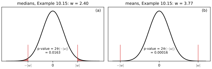
fig_10_4. Download: PDF · SVGTheorem 10.14 (p-values are uniform under the null) p. 158
If the test statistic has a continuous distribution, then under \(H_0:\th=\th_0\) the p-value is \(\Unif(0,1)\). Rejecting when the p-value is below \(\alpha\) therefore has type I error probability \(\alpha\). Under \(H_1\) the p-value tends to be smaller.
Filling the gap 10.7: proof (Exercise 10.2), the discrete case, and the distribution under the alternative p. 158
Let \(F\) be the null cdf of \(T\) and \(p=\bar F(T)\) with \(\bar F(t)=\P_{\th_0}(T\ge t)\). (a) If \(F\) is continuous, \(p\sim\Unif(0,1)\) under \(H_0\). (b) In general \(p\) is super-uniform: \(\P_{\th_0}(p\le u)\le u\) for every \(u\in[0,1]\), so a test that rejects when \(p\le\alpha\) has level \(\alpha\). (c) For the two-sided Wald test of a Normal mean with \(\delta=\sqrt n(\th-\th_0)/\sigma\), \[ \P_\th(p\le u)=1-\Phi(z_{u/2}-\delta)+\Phi(-z_{u/2}-\delta), \] the power at level \(u\); its density is decreasing in \(u\) when \(\delta\ne0\), piling up near 0.
Proof
(b) first. Fix \(u\in(0,1)\) and let \(t_u=\inf\{t:\bar F(t)\le u\}\). Because \(\bar F\) is non-increasing and left-continuous (\(\bar F(t)=\P(T\ge t)\) and the events \(\{T\ge t\}\) decrease to \(\{T\ge t_0\}\) as \(t\uparrow t_0\)), the set \(\{t:\bar F(t)\le u\}\) is an interval whose left end \(t_u\) may or may not belong to it. If it does, \(\{p\le u\}=\{T\ge t_u\}\) and \(\P(p\le u)=\bar F(t_u)\le u\). If it does not, \(\{p\le u\}=\{T>t_u\}\) and \(\P(T>t_u)=\lim_{t\downarrow t_u}\bar F(t)\le u\). (a) If \(F\) is continuous, \(\bar F=1-F\) is continuous and takes every value in \((0,1)\), so \(\bar F(t_u)=u\) and the inequality is an equality: \(\P(p\le u)=u\). Equivalently, \(1-p=F(T)\) is the probability integral transform of a continuous variable, which is uniform (Result 2.4). (c) \(p\le u\iff|W|\ge z_{u/2}\), and \(W=Z+\delta\) exactly; differentiating in \(u\) with \(\d z_{u/2}/\d u=-1/(2\phi(z_{u/2}))\) gives the density \[ \{\phi(z_{u/2}-\delta)+\phi(z_{u/2}+\delta)\}/\{2\phi(z_{u/2})\}=e^{-\delta^2/2}\cosh(\delta z_{u/2}), \] which decreases in \(u\) because \(z_{u/2}\) does. ∎
For a composite null, apply (b) at each \(\th\in\Theta_0\) with the p-value of Theorem 10.12, which is at least \(\bar F_\th(T)\): super-uniformity holds for every \(\th\in\Theta_0\). Discreteness makes p-values conservative only when ties are counted with "\(\ge\)"; with "\(>\)" they can be anti-conservative (Filling the gap 10.11).
See also: the first-year notes, Theorem 4.1; Statistical Methods for Modern Biology, Result 6.1; Applied Statistical Learning, Result 13.1.
Filling the gap 10.8: a p-value is not \(\P(H_0\given\text{data})\): the test as a diagnostic test p. 157
Think of each null hypothesis that a field tests as a patient screened for a disease ("the effect is real"): the test's size \(\alpha\) is the false-positive rate, its power \(1-\gamma\) the sensitivity, and the fraction \(\pi_0\) of true nulls among the hypotheses tested the base rate of "no disease". (a) By Bayes' theorem,
\[ \P(H_0\text{ true}\given\text{rejected at level }\alpha)=\frac{\pi_0\,\alpha}{\pi_0\,\alpha+(1-\pi_0)(1-\gamma)}, \]which can be far above \(\alpha\): with \(\pi_0=0.8\) and power 0.5 it is 0.29. (b) Even for a single study, conditioning on the observed \(z\) rather than on "\(p\le0.05\)": for a Normal statistic and any prior on the alternative, the Bayes factor in favour of \(H_0\) is at least \(e^{-z^2/2}\); at \(z=1.96\) (\(p=0.05\)) and prior odds 1, \(\P(H_0\given z)\ge1/(1+e^{1.92})=0.128\).
Proof
(a) Bayes' theorem (Theorem 1.17) with the partition \(\{H_0,H_1\}\): \[ \P(H_0\given\text{rej})=\P(\text{rej}\given H_0)\P(H_0)/\P(\text{rej}), \] with \(\P(\text{rej}\given H_0)=\alpha\), \(\P(\text{rej}\given H_1)=1-\gamma\). This is exactly the diagnostic-test calculation of Filling the gap 1.11: a rare condition and an imperfect test make most positives false.
(b) Let \(z\) be an observation of \(Z\sim N(\mu,1)\), \(H_0:\mu=0\), and let \(\pi\) be any prior on \(\mu\ne0\) under \(H_1\). The marginal density under \(H_1\) is \[ \int\phi(z-\mu)\,\pi(\d\mu)\le\sup_\mu\phi(z-\mu)=\phi(0). \] So the Bayes factor \[ B=\phi(z)/\int\phi(z-\mu)\pi(\d\mu)\ge\phi(z)/\phi(0)=e^{-z^2/2}, \] and with prior probability 1/2 on each hypothesis \[ \P(H_0\given z)=B/(1+B)\ge e^{-z^2/2}/(1+e^{-z^2/2}). \] At \(z=1.96\), \(e^{-1.92}=0.146\) and the bound is 0.128; any reasonable prior (not concentrated at the observed \(z\)) gives a much larger value. ∎
The p-value is a statement about the data under \(H_0\) (how surprising they would be), not about \(H_0\) given the data. The two coincide in no generality, and the gap is largest exactly where p-values are most often quoted, just below 0.05.
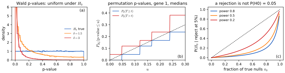
fig_10_s2. Download: PDF · SVGExample 10.15 (the cholesterol data) pp. 158–159
Return to the plasma cholesterol data of Example 7.15: 51 patients without heart disease (mean 195.27, \(\hse=5.0\)) and 320 with narrowed arteries (mean 216.19, \(\hse=2.4\)). For the difference of means,
\[ W=\frac{216.19-195.27}{\sqrt{5.0^2+2.4^2}}=\frac{20.92}{5.55}=3.77,\qquad\text{p-value}=2\Phi(-3.77)=0.00016, \]very strong evidence of a difference (the book prints 3.78 and 0.0002; see the notes on the book). For the difference of medians, \(212.5-194=18.5\) with a bootstrap standard error of 7.7, so \(W=2.40\) and the p-value is \(2\Phi(-2.40)=0.016\): strong evidence. (The raw data are not distributed with the book, so the numbers are recomputed from the published summaries.)
10.3 The \(\chi^2\) Distribution
p. 159 If \(Z_1,\dots,Z_k\) are independent \(N(0,1)\) and \(V=\sum_{i=1}^kZ_i^2\), then \(V\) has the \(\chi^2\) distribution with \(k\) degrees of freedom, \(V\sim\chisq{k}\), with density
\[ f(v)=\frac{v^{k/2-1}e^{-v/2}}{2^{k/2}\Gamma(k/2)},\qquad v>0. \]The upper \(\alpha\) quantile is \(\chisq{k,\alpha}=F^{-1}(1-\alpha)\), so \(\P(\chisq{k}>\chisq{k,\alpha})=\alpha\); for instance \(\chisq{1,0.05}=3.841=1.96^2\) and \(\chisq{3,0.05}=7.815\).
Filling the gap 10.9: the density, and "it can be shown that \(\E(V)=k\) and \(\V(V)=2k\)" p. 159
(a) \(Z^2\) has the Gamma density with shape \(1/2\) and scale 2; (b) a sum of independent Gamma variables with a common scale is Gamma with the shapes added, so \(V\sim\) Gamma\((k/2,2)\), which is the density above; (c) \(\E V=k\), \(\V V=2k\); (d) if \(V_1\sim\chisq{a}\) and \(V_2\sim\chisq{b}\) are independent, \(V_1+V_2\sim\chisq{a+b}\).
Proof
(a) For \(v>0\), \(\P(Z^2\le v)=\Phi(\sqrt v)-\Phi(-\sqrt v)\); differentiating, the density is \[ 2\phi(\sqrt v)\cdot\tfrac1{2\sqrt v}=v^{-1/2}e^{-v/2}/\sqrt{2\pi}, \] which is the Gamma\((1/2,2)\) density because \(\Gamma(1/2)=\sqrt\pi\). (b) The moment generating function of Gamma\((a,2)\) is \((1-2t)^{-a}\) for \(t<1/2\); by independence the MGF of \(V\) is \((1-2t)^{-k/2}\), the MGF of Gamma\((k/2,2)\), and MGFs finite near 0 determine the distribution. (c) \(\E Z^2=1\) and \(\E Z^4=3\), so \(\V Z^2=2\); add over the \(k\) independent terms. (d) Multiply the MGFs. ∎
The same facts, with the Gamma integral, are in Result 2.10 of Chapter 2; the first-year notes prove them in Theorem 0.8. One more fact is used repeatedly below: if \(Y\sim N(0,P)\) in \(\R^k\) with \(P\) an orthogonal projection of rank \(d\), then \(\|Y\|^2\sim\chisq{d}\). Indeed \(P=Q\,\mathrm{diag}(1,\dots,1,0,\dots,0)\,Q^\T\) with \(Q\) orthogonal and \(d\) ones, so \(Q^\T Y\) has \(d\) independent \(N(0,1)\) coordinates and \(k-d\) zero ones, and \(\|Y\|^2=\|Q^\T Y\|^2\).
10.4 Pearson's \(\chi^2\) Test For Multinomial Data
p. 160 If \(X=(X_1,\dots,X_k)\sim\) Multinomial\((n,p)\), the MLE of \(p\) is \(\hat p=X/n\). For a fixed vector \(p_0\) we test \(H_0:p=p_0\) against \(H_1:p\ne p_0\).
Definition 10.16 (Pearson's \(\chi^2\) statistic) p. 160
\[ T=\sum_{j=1}^k\frac{(X_j-np_{0j})^2}{np_{0j}}=\sum_{j=1}^k\frac{(X_j-E_j)^2}{E_j}, \]where \(E_j=\E(X_j)=np_{0j}\) is the expected count under \(H_0\).
Theorem 10.17 (Pearson) p. 160
Under \(H_0\), \(T\convd\chisq{k-1}\). Hence rejecting when \(T>\chisq{k-1,\alpha}\) has asymptotic level \(\alpha\), and the p-value is \(\P(\chisq{k-1}>t)\) for the observed \(t\).
Filling the gap 10.10: proof of Pearson's theorem p. 160
Assume every \(p_{0j}>0\). The statistic is the squared length of a vector that converges to a Normal vector with a projection covariance of rank \(k-1\); the missing dimension is the constraint \(\sum_jX_j=n\).
Proof
Write \(X=\sum_{i=1}^n\xi_i\), with \(\xi_i\) the indicator vector of the category of observation \(i\): iid, mean \(p_0\), covariance \(\Sigma=\mathrm{diag}(p_0)-p_0p_0^\T\) (Filling the gap 3.6). By the multivariate central limit theorem (Theorem 5.12), \((X-np_0)/\sqrt n\convd N(0,\Sigma)\). Let \(D=\mathrm{diag}(p_0)\) and \(U=D^{-1/2}(X-np_0)/\sqrt n\), so that \(T=\|U\|^2\). By the continuous mapping theorem, \(U\convd N(0,D^{-1/2}\Sigma D^{-1/2})\), and
\[ D^{-1/2}\Sigma D^{-1/2}=I-uu^\T,\qquad u=(\sqrt{p_{01}},\dots,\sqrt{p_{0k}})^\T,\quad \|u\|^2=\textstyle\sum_jp_{0j}=1, \]the orthogonal projection onto the \((k-1)\)-dimensional complement of \(u\). By the fact at the end of Filling the gap 10.9 and the continuity of \(y\mapsto\|y\|^2\), \(T=\|U\|^2\convd\chisq{k-1}\). ∎
The same theorem with a different proof (and the exact null mean \(k-1\)) is in Statistical Methods for Modern Biology, Filling the gap 2.6 and Result 1.9. The approximation is usually trusted when every \(E_j\) is at least about 5; Figure 10.S3(b) shows it is excellent for Mendel's counts.
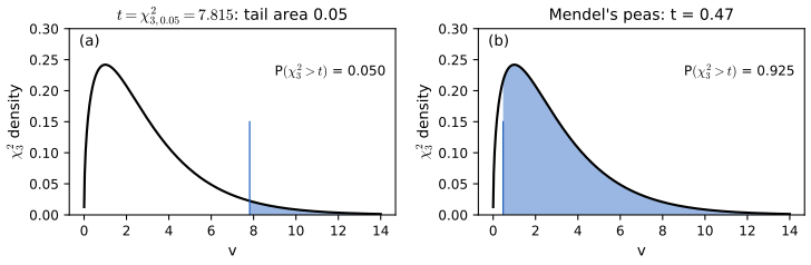
fig_10_5. Download: PDF · SVGExample 10.18 (Mendel's peas) p. 161
Crossing round-yellow with wrinkled-green peas, Mendel's theory predicts the four progeny types (round yellow, wrinkled yellow, round green, wrinkled green) with probabilities \(p_0=(9/16,3/16,3/16,1/16)\). In \(n=556\) plants he observed \(X=(315,101,108,32)\). The expected counts are \((312.75,104.25,104.25,34.75)\) and
\[ T=\frac{2.25^2}{312.75}+\frac{3.25^2}{104.25}+\frac{3.75^2}{104.25}+\frac{2.75^2}{34.75}=0.470,\qquad\text{p-value}=\P(\chisq{3}>0.470)=0.925. \]The data do not contradict the theory. The book adds two remarks. A test is the wrong tool for proving \(H_0\): failing to reject may only reflect low power, and a confidence set for the distance between \(p\) and \(p_0\) would say more. And Mendel's results have been called "too good": here \(\P(\chisq{3}\le0.470)=0.075\), so a fit this close happens one time in 13 and is unremarkable on its own; the suspicion (Fisher, 1936) came from pooling many of Mendel's experiments, whose combined agreement with theory was closer than chance would usually allow.
See also: Statistical Methods for Modern Biology, the Pearson statistic demo and the chi-square power demo.
10.5 The Permutation Test
pp. 161–162 The permutation test checks whether two samples come from the same distribution, \(H_0:F_X=F_Y\) against \(H_1:F_X\ne F_Y\), with \(X_1,\dots,X_m\sim F_X\) and \(Y_1,\dots,Y_n\sim F_Y\) independent. It is exact: its size is controlled for every sample size, with no large-sample approximation. Take a statistic such as \(T=|\overline X_m-\overline Y_n|\); compute it for all \(N!\) orderings of the pooled data \((X_1,\dots,X_m,Y_1,\dots,Y_n)\), \(N=m+n\), treating the first \(m\) values as the \(X\) sample. Under \(H_0\) all orderings are equally likely, so the distribution putting mass \(1/N!\) on each value is the permutation distribution of \(T\), and the p-value is the permutation probability of a value as extreme as the observed \(t_{\rm obs}\). (Orderings that differ only within the two groups give the same \(T\), so it suffices to list the \(\binom Nm\) splits into a group of size \(m\) and a group of size \(n\).)
Algorithm 10.A (permutation test, Monte Carlo version) p. 163
- Compute the observed statistic \(t_{\rm obs}=T(X_1,\dots,X_m,Y_1,\dots,Y_n)\).
- Permute the pooled data at random and recompute the statistic.
- Repeat step 2 \(B\) times, giving \(T_1,\dots,T_B\).
- The approximate p-value is \((1+\#\{b:T_b\ge t_{\rm obs}\})/(B+1)\).
Step 4 is not the book's formula, \(B^{-1}\sum_b\I(T_b>t_{\rm obs})\); Filling the gap 10.11 explains why the version given here (counting ties and adding one) is the one that guarantees the level.
p. 162 Example 10.19 (a toy example). With \((X_1,X_2,Y_1)=(1,9,3)\) and \(T=|\overline X-\overline Y|\), the observed value is \(|5-3|=2\). The six orderings give \(T=2,2,7,7,5,5\). The book reports \(\P(T>2)=4/6\); counting the observed value as "at least as extreme", as Theorem 10.12 does, the p-value is \(\P(T\ge2)=1\): the observed split is the least extreme possible.
Example 10.20 (DNA microarrays) p. 163
Expression levels (log-ratios) of 2,638 genes were measured on ten patients with one of two types of liver cancer (Efron et al., 2001). For gene 1 the Type I patients give \(230,-1350,-1580,-400,-760\) and the Type II patients \(970,110,-50,-190,-200\). The medians are \(-760\) and \(-50\), so \(T=|\hat\nu_1-\hat\nu_2|=710\). The book estimates the permutation p-value by simulation as 0.045 and concludes that there is evidence of a difference at the 5% level.
With ten patients there are only \(\binom{10}{5}=252\) splits, so the p-value can be computed exactly. Thirty splits give \(T\ge710\), twelve give \(T>710\), and eighteen give exactly 710 (the medians of five values are data values, so ties are common). The exact p-value is \(30/252=0.119\); the book's 0.045 is a simulation estimate of \(12/252=0.048\), the probability of a strictly larger value. Counting ties correctly, gene 1 shows no significant difference at the 5% level. For gene 2, the exact p-value is \(108/252=0.429\).
Filling the gap 10.11: why the permutation test is exact, and why ties must count pp. 161–163, footnote 4
Let \(Z=(X_1,\dots,X_m,Y_1,\dots,Y_n)\) and, for a permutation \(\pi\) of \(\{1,\dots,N\}\), \(Z_\pi=(Z_{\pi(1)},\dots,Z_{\pi(N)})\). Define
\[ p_\ge(Z)=\frac1{N!}\sum_\pi\I\{T(Z_\pi)\ge T(Z)\},\qquad p_>(Z)=\frac1{N!}\sum_\pi\I\{T(Z_\pi)>T(Z)\}. \](a) Under \(H_0\), \(Z\) is exchangeable: \(Z_\pi\) has the same distribution as \(Z\) for every \(\pi\). (b) If \(Z\) is exchangeable, \(\P(p_\ge(Z)\le u)\le u\) for every \(u\in[0,1]\), whatever \(F\) is (continuous or not) and whatever \(N\) is. (c) The Monte Carlo p-value \(\hat p=(1+\#\{b:T_b\ge t_{\rm obs}\})/(B+1)\) also satisfies \(\P(\hat p\le u)\le u\). (d) \(p_>\) does not: it equals 0 with positive probability whenever the largest permutation value is attained by the observed ordering.
Proof
(a) Under \(H_0\) the \(N\) coordinates of \(Z\) are iid from \(F=F_X=F_Y\), and an iid vector has a permutation-invariant joint law.
(b) Let \(\Pi\) be a uniformly random permutation independent of \(Z\). By exchangeability \(Z_\Pi\) has the law of \(Z\), so \[ \P(p_\ge(Z)\le u)=\P(p_\ge(Z_\Pi)\le u)=\E\big[\P(p_\ge(Z_\Pi)\le u\given Z)\big]. \] Fix \(Z=z\) and write \(t_\pi=T(z_\pi)\). Because \(\sigma\mapsto\pi\circ\sigma\) is a bijection of the permutation group,
\[ p_\ge(z_\pi)=\frac1{N!}\#\{\sigma:\ t_{\pi\circ\sigma}\ge t_\pi\}=\frac1{N!}\#\{\sigma':\ t_{\sigma'}\ge t_\pi\}=\bar G(t_\pi), \]where \(\bar G(t)=\P(t_\Pi\ge t)\) is the upper tail function of the discrete uniform distribution of \(t_\Pi\) given \(z\). So, given \(z\), \(p_\ge(z_\Pi)\) is the tail-function transform of the random variable \(t_\Pi\), which is super-uniform by Filling the gap 10.7(b): \(\P(p_\ge(z_\Pi)\le u\given Z=z)\le u\). Taking expectations proves (b). This is the precise content of the book's footnote 4: given the unordered set of values, the labelling is uniform over the permutations.
(c) Conditionally on the multiset of values, \(T(Z),T_1,\dots,T_B\) are \(B+1\) iid draws from the permutation distribution (the first by exchangeability, the others by construction), hence exchangeable. The rank of \(T(Z)\) among them, counting ties against it, is then super-uniform on \(\{1,\dots,B+1\}\), and \(\hat p\) is that rank divided by \(B+1\).
(d) If the largest value \(t_{\max}\) of \(t_\pi\) is attained by \(k\) of the \(N!\) orderings, then \(p_>(z_\Pi)=0\) with conditional probability \(k/N!>0\), so \(\P(p_>\le0)>0\) and the test "reject if \(p_>\le\alpha\)" has size above \(\alpha\) for small \(\alpha\). For the gene 1 values, \(\P_0(p_>=0)=12/252=0.048\) and \(\P_0(p_>\le0.05)=0.12\) (Figure 10.S2(b)). ∎
Two consequences. First, for continuous data with no ties, \(p_\ge\) is exactly uniform on the grid \(\{1,2,\dots\}/\binom Nm\) (for the symmetric statistic with \(m=n\), on its even multiples), so at \(m=n=5\) the level 0.05 test has size \(12/252=0.0476\) exactly; the smallest attainable p-value is \(2/252\), and with \(m=n=3\) it is \(2/20=0.1\): no rejection at 5% is possible. Second, exactness is relative to the null \(F_X=F_Y\). If the means are equal but the spreads differ, the permutation test of \(|\overline X-\overline Y|\) is not a valid test of equal means (Figure 10.S4(c)). Finally, for fixed pooled data the pooled two-sample \(t\) statistic is an increasing function of \(|\overline X-\overline Y|\) (the total sum of squares does not change under relabelling), so permuting \(|t|\) and permuting \(|\overline X-\overline Y|\) give the same test.
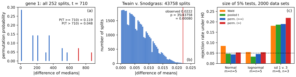
fig_10_s4. Download: PDF · SVGSee also: Statistical Methods for Modern Biology, Result 6.4 and its permutation demo; Applied Statistical Learning, Result 13.6 and the Khan permutation demo; Statistical Learning: Theory and Methods, Filling the gap 18.8.
p. 164 In large samples the permutation test usually agrees with a test based on large-sample theory, so it is most useful for small samples. It also needs no estimate of a standard error, which is why it is convenient for statistics like the difference of medians.
10.6 The Likelihood Ratio Test
p. 164 The Wald test handles one scalar parameter at a time; the likelihood ratio test handles a vector.
Definition 10.21 (likelihood ratio statistic) p. 164
To test \(H_0:\th\in\Theta_0\) against \(H_1:\th\notin\Theta_0\), let
\[ \lambda=2\log\frac{\sup_{\th\in\Theta}L(\th)}{\sup_{\th\in\Theta_0}L(\th)}=2\log\frac{L(\hth)}{L(\hth_0)}, \]where \(\hth\) is the MLE and \(\hth_0\) the MLE restricted to \(\Theta_0\).
The numerator maximises over all of \(\Theta\) rather than over \(\Theta_0^c\). This changes nothing when the unrestricted maximum lies outside \(\Theta_0\), and it makes \(\lambda\ge0\) and its theory simpler.
Theorem 10.22 (Wilks) p. 164
Let \(\th=(\th_1,\dots,\th_q,\th_{q+1},\dots,\th_r)\) and \[ \Theta_0=\{\th:(\th_{q+1},\dots,\th_r)=(\th_{0,q+1},\dots,\th_{0,r})\}. \] Under \(H_0:\th\in\Theta_0\),
\[ \lambda\convd\chisq{r-q}, \]where \(r-q\) is the dimension of \(\Theta\) minus the dimension of \(\Theta_0\) (the number of constraints). The p-value is \(\P(\chisq{r-q}>\lambda)\). For instance, testing \(\th_4=\th_5=0\) in a five-parameter model uses \(\chisq{2}\).
Filling the gap 10.12: why \(\lambda\) is asymptotically \(\chi^2_{r-q}\) (sketch of proof), and why it agrees with Pearson's statistic pp. 164–165
Assume the regularity conditions of Chapter 9: iid data, \(\Theta\) open in \(\R^r\), the true value \(\th^\ast\in\Theta_0\) interior, a log-likelihood three times differentiable with dominated third derivatives, Fisher information \(\mathcal I=\mathcal I(\th^\ast)\) positive definite, and consistent unrestricted and restricted MLEs. Then \(\lambda\convd\chisq{r-q}\). For multinomial data, in addition, \(\lambda-T\convp0\) with \(T\) Pearson's statistic.
Proof sketch
Step 1 (local quadratic approximation). Let \(\ell\) be the log-likelihood, \(S_n=n^{-1/2}\nabla\ell(\th^\ast)\) the normalised score, and \(h\in\R^r\) a local parameter. A second-order Taylor expansion, with the third-order remainder controlled by the domination condition and the law of large numbers for \(-n^{-1}\nabla^2\ell(\th^\ast)\convp\mathcal I\), gives, uniformly for \(h\) in compact sets,
\[ \ell(\th^\ast+h/\sqrt n)-\ell(\th^\ast)=h^\T S_n-\tfrac12h^\T\mathcal Ih+o_P(1),\qquad S_n\convd Y\sim N(0,\mathcal I) \](the score has mean zero and covariance \(\mathcal I\), and the CLT applies).
Step 2 (maximise the quadratic). Both MLEs are \(\sqrt n\)-consistent under \(H_0\) (Chapter 9), so the maxima of \(\ell\) over \(\Theta\) and \(\Theta_0\) are attained at local parameters that are bounded in probability, and the maximum of \(\ell\) is the maximum of the quadratic up to \(o_P(1)\). Over all \(h\in\R^r\) the maximum of \(h^\T s-\frac12h^\T\mathcal Ih\) is \(\frac12s^\T\mathcal I^{-1}s\). Under \(H_0\), \(\Theta_0\) corresponds to \(h\in L=\{Ag:g\in\R^q\}\) with \(A=\binom{I_q}{0}\), and the maximum over \(L\) is \(\frac12s^\T A(A^\T\mathcal IA)^{-1}A^\T s\). Hence
\[ \lambda=S_n^\T\big[\mathcal I^{-1}-A(A^\T\mathcal IA)^{-1}A^\T\big]S_n+o_P(1). \]Step 3 (identify the limit). With \(W=\mathcal I^{-1/2}Y\sim N(0,I_r)\) and \(B=\mathcal I^{1/2}A\), the limit is
\[ W^\T\big[I_r-B(B^\T B)^{-1}B^\T\big]W, \]the squared length of the projection of a standard Normal vector onto the orthogonal complement of the \(q\)-dimensional column space of \(B\). By the fact in Filling the gap 10.9 it is \(\chisq{r-q}\); the continuous mapping theorem and Slutsky's theorem carry the limit through. ∎
Agreement with Pearson. For multinomial counts write \(D_j=X_j-E_j\), which is \(O_P(\sqrt n)\), and expand \[ 2(E+D)\log(1+D/E)=2D+D^2/E+O(|D|^3/E^2). \] Summing over \(j\) and using \(\sum_jD_j=0\),
\[ \lambda=2\sum_jX_j\log\frac{X_j}{E_j}=\sum_j\frac{D_j^2}{E_j}+O_P(n^{-1/2})=T+o_P(1). \]This is why Examples 10.18 and 10.23 give 0.470 and 0.475. The same expansion shows that the Wald, score and likelihood ratio statistics are asymptotically equivalent (Exercise 10.16), and Statistical Methods for Modern Biology works the Wald and likelihood ratio tests out for Poisson regression in Filling the gap 8.13. The regularity conditions matter: if \(\th^\ast\) lies on the boundary of \(\Theta\) (testing that a variance component is zero, or the number of components of a mixture), the limit is not \(\chi^2\).
Example 10.23 (Mendel's peas revisited) p. 165
For the multinomial, \(L(p)\propto\prod_jp_j^{X_j}\) and \(\hat p_j=X_j/n\), so
\[ \lambda=2\sum_{j=1}^4X_j\log\frac{\hat p_j}{p_{0j}}=2\Big[315\log\frac{315/556}{9/16}+101\log\frac{101/556}{3/16}+108\log\frac{108/556}{3/16}+32\log\frac{32/556}{1/16}\Big]=0.475. \]The full model has three free parameters (four probabilities summing to one) and the null none, so \(\lambda\) is compared with \(\chisq{3}\): p-value \(0.924\). The conclusion matches Pearson's test, as Filling the gap 10.12 predicts for large \(n\).
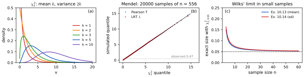
fig_10_s3. Download: PDF · SVG10.7 Multiple Testing
pp. 165–166 In Example 10.20 there were really 2,638 genes. Testing each at level \(\alpha\) keeps the chance of a false rejection at \(\alpha\) for each gene, but the chance of at least one false rejection among thousands of true nulls is close to 1. Consider \(m\) tests of \(H_{0i}\) against \(H_{1i}\) with p-values \(P_1,\dots,P_m\).
Algorithm 10.B (the Bonferroni method) p. 166
Reject \(H_{0i}\) if \(P_i<\alpha/m\).
Theorem 10.24 (Bonferroni) p. 166
With the Bonferroni method, the probability of falsely rejecting any null hypothesis (the family-wise error rate, FWER) is at most \(\alpha\).
Filling the gap 10.13: the Bonferroni bound, sharpened, and what it does not need p. 166
Let \(\mathcal H_0\) be the set of the \(m_0\) true nulls and assume only that each true-null p-value is super-uniform (Filling the gap 10.7). Then \(\FWER\le m_0\alpha/m\le\alpha\), with no assumption on the dependence between the tests. Under independence and exactly uniform null p-values, \(\FWER=1-(1-\alpha/m)^{m_0}\), which is close to the bound: for \(m=m_0=50\) and \(\alpha=0.05\), 0.0488.
Proof
A false rejection can only happen for a true null, so the event is \(\bigcup_{i\in\mathcal H_0}\{P_i<\alpha/m\}\). By the union bound (Boole's inequality, Chapter 1), its probability is at most \[ \sum_{i\in\mathcal H_0}\P(P_i<\alpha/m)\le m_0\alpha/m. \] The book's proof sums over all \(m\) hypotheses and uses \(\P(R_i)=\alpha/m\) for each; the events \(R_i\) of a false rejection are empty for false nulls, so the sum over true nulls is the accurate one, and "\(=\)" becomes "\(\le\)" for discrete p-values. Under independence, the complement "no true null rejected" has probability \(\prod_{i\in\mathcal H_0}(1-\alpha/m)\). ∎
Holm's step-down procedure controls the FWER under the same conditions and rejects at least as much (Applied Statistical Learning, Result 13.4).
p. 166 Example 10.25. For the 2,638 genes at \(\alpha=0.05\), Bonferroni rejects a gene only if its p-value is below \(0.05/2638=1.895\times10^{-5}\).
pp. 166–167 Bonferroni guards against even one false rejection, which is very conservative when thousands of hypotheses are screened for follow-up. A less demanding target is the proportion of false discoveries.
Definition 10.C (false discovery proportion and rate) pp. 166–167, Table 10.2
For a rule that rejects some hypotheses, let \(V\) be the number of true nulls rejected, \(S\) the number of false nulls rejected, \(R=V+S\) the number of rejections, \(U\) and \(T\) the numbers of true and false nulls retained, so that \(U+V=m_0\), \(T+S=m_1=m-m_0\). The false discovery proportion is \(\FDP=V/R\) if \(R>0\) and 0 if \(R=0\), and the false discovery rate is \(\FDR=\E(\FDP)\).
| \(H_0\) not rejected | \(H_0\) rejected | total | |
|---|---|---|---|
| \(H_0\) true | \(U\) | \(V\) | \(m_0\) |
| \(H_0\) false | \(T\) | \(S\) | \(m_1\) |
| total | \(m-R\) | \(R\) | \(m\) |
Algorithm 10.C (the Benjamini–Hochberg method) p. 167, (10.8)
- Order the p-values: \(P_{(1)}<\dots<P_{(m)}\).
- Let \(\ell_i=i\alpha/(C_mm)\) and
- where \(C_m=1\) if the p-values are independent and \(C_m=\sum_{i=1}^m1/i\) otherwise. Let \(T=P_{(R)}\), the BH rejection threshold.
- Reject every \(H_{0i}\) with \(P_i\le T\) (and none if no \(i\) satisfies (10.8)).
Theorem 10.26 (Benjamini and Hochberg) p. 167
Whatever the number of true nulls and whatever the distribution of the p-values of the false nulls,
\[ \FDR=\E(\FDP)\le\frac{m_0}m\alpha\le\alpha. \]Filling the gap 10.14: proof of the Benjamini–Hochberg theorem, with and without independence p. 167
Assume the true-null p-values are \(\Unif(0,1)\). (a) If the true-null p-values are independent of each other and of the false-null p-values, BH with \(C_m=1\) has \(\FDR=m_0\alpha/m\) exactly. (b) Under arbitrary dependence, BH with \(C_m=\sum_{i\le m}1/i\) has \(\FDR\le m_0\alpha/m\).
Proof
A reformulation. Let \(\alpha'=\alpha/C_m\) and \(N(r)=\#\{j:P_j\le r\alpha'/m\}\). Then \(P_{(r)}\le r\alpha'/m\) if and only if \(N(r)\ge r\), so \(R=\max\{r:N(r)\ge r\}\) (with probability one the strict and weak inequalities agree, the p-values of true nulls being continuous; ties among false-null p-values do not matter below), and hypothesis \(i\) is rejected if and only if \(P_i\le R\alpha'/m\). With \(V_i=\I\{i\text{ rejected}\}\) for \(i\in\mathcal H_0\),
\[ \FDP=\sum_{i\in\mathcal H_0}\frac{V_i}{\max(R,1)}=\sum_{i\in\mathcal H_0}\sum_{k=1}^m\frac1k\I\{P_i\le k\alpha'/m,\ R=k\}. \](a) Independence. Fix \(i\in\mathcal H_0\) and let \(R^{(i)}\) be the number of rejections when \(P_i\) is replaced by 0, a function of the other p-values only. If \(P_i\le k\alpha'/m\), then \(N(r)\) is unchanged by this replacement for every \(r\ge k\), so \(R=k\) if and only if \(R^{(i)}=k\) (both say: \(N(k)\ge k\) and \(N(r)<r\) for all \(r>k\)). Therefore, using the independence of \(P_i\) from \(R^{(i)}\) and \(\P(P_i\le k\alpha/m)=k\alpha/m\),
\[ \E\frac{V_i}{\max(R,1)}=\sum_{k=1}^m\frac1k\P\big(P_i\le\tfrac{k\alpha}m\big)\P\big(R^{(i)}=k\big)=\frac\alpha m\sum_{k=1}^m\P\big(R^{(i)}=k\big)=\frac\alpha m, \]because \(R^{(i)}\ge1\) always (the p-value 0 is rejected). Summing over the \(m_0\) true nulls gives \(\FDR=m_0\alpha/m\).
(b) Any dependence. Split \((0,k\alpha'/m]\) into the intervals \(I_j=((j-1)\alpha'/m,\ j\alpha'/m]\), \(j\le k\). Then
\[ \sum_{k=1}^m\frac1k\I\{P_i\le\tfrac{k\alpha'}m,R=k\}=\sum_{j=1}^m\I\{P_i\in I_j\}\sum_{k\ge j}\frac{\I\{R=k\}}k\le\sum_{j=1}^m\frac{\I\{P_i\in I_j\}}j, \]since at most one \(\I\{R=k\}\) is 1 and \(1/k\le1/j\) for \(k\ge j\). Taking expectations, \(\P(P_i\in I_j)=\alpha'/m\) for a uniform \(P_i\), so the expectation is at most \[ (\alpha'/m)\sum_{j\le m}1/j=(\alpha'/m)C_m=\alpha/m. \] Summing over \(\mathcal H_0\) gives \(\FDR\le m_0\alpha/m\). No independence was used. ∎
Part (a) is the original theorem of Benjamini and Hochberg (1995) and part (b) is due to Benjamini and Yekutieli (2001), who also showed that \(C_m=1\) suffices under positive regression dependence; in the simulation of Figure 10.S5 equicorrelated statistics keep the FDR of plain BH below \(m_0\alpha/m\). Statistical Methods for Modern Biology gives another complete proof (Result 6.6), and Applied Statistical Learning a short one (Filling the gap 13.10).
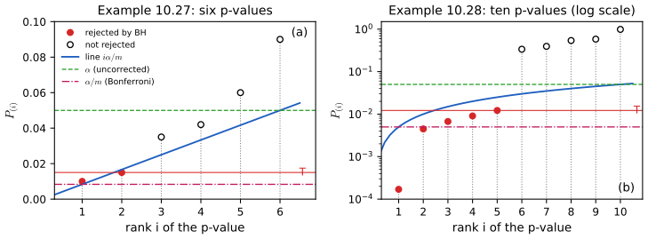
fig_10_6. Download: PDF · SVGpp. 167–168 Example 10.27 describes Figure 10.6(a). Example 10.28: ten independent tests give the ordered p-values 0.00017, 0.00448, 0.00671, 0.00907, 0.01220, 0.33626, 0.39341, 0.53882, 0.58125, 0.98617. At \(\alpha=0.05\), Bonferroni rejects the p-values below 0.005, the first two. For BH, \(\ell_i=0.005i\), and \(P_{(5)}=0.0122<0.025\) while \(P_{(6)}=0.336>0.030\); the largest \(i\) with \(P_{(i)}<\ell_i\) is 5, so BH rejects the first five. If dependence is allowed (\(C_{10}=2.929\)), the line becomes \(0.00171i\) and only the first hypothesis is rejected.
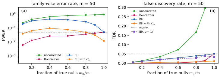
fig_10_s5. Download: PDF · SVGSee also: Statistical Methods for Modern Biology, Section 6.9 and the FDR demo on 33,469 genes; Applied Statistical Learning, Section 13.4 and the BH demo; Statistical Learning: Theory and Methods, Result 18.12.
10.8 Goodness-of-fit Tests
pp. 168–169 Testing also arises when we ask whether data come from an assumed parametric model \(\mathfrak F=\{f(x;\th):\th\in\Theta\}\), \(\th=(\th_1,\dots,\th_s)\). Divide the line into \(k\) disjoint intervals \(I_1,\dots,I_k\), let \(p_j(\th)=\int_{I_j}f(x;\th)\,\d x\), and let \(N_j\) be the number of observations in \(I_j\). The counts have the multinomial likelihood \(\mathcal Q(\th)=\prod_{j=1}^kp_j(\th)^{N_j}\); its maximiser \(\tth\) is the grouped-data MLE, and
\[ Q=\sum_{j=1}^k\frac{(N_j-np_j(\tth))^2}{np_j(\tth)}. \tag{10.9} \]Theorem 10.29 (goodness of fit with estimated parameters) p. 169
Under \(H_0\): the data are iid from some member of \(\mathfrak F\), \(Q\convd\chisq{k-1-s}\), and the approximate p-value is \(\P(\chisq{k-1-s}>q)\) for the observed \(q\). If \(\tth\) is replaced by the ordinary MLE \(\hth\) computed from the raw data, the limit is no longer \(\chisq{k-1-s}\); by a theorem of Chernoff and Lehmann (1954) the p-value then lies approximately between those computed from \(\chisq{k-1-s}\) and \(\chisq{k-1}\).
Filling the gap 10.15: one degree of freedom per estimated parameter, and the Chernoff–Lehmann bound p. 169
Assume \(p_j(\th)>0\), the map \(\th\mapsto p(\th)\) is twice continuously differentiable with a Jacobian of full rank \(s<k-1\), and the true \(\th^\ast\) is interior. (a) With \(\tth\), \(Q\convd\chisq{k-1-s}\). (b) With the raw-data MLE \(\hth\), \[ Q\convd\sum_{j=1}^{k-1-s}Z_j^2+\sum_{j=1}^s\lambda_jZ_{k-1-s+j}^2 \] with iid \(Z_j\sim N(0,1)\) and constants \(\lambda_j\in[0,1)\); hence \(Q\) is asymptotically stochastically between \(\chisq{k-1-s}\) and \(\chisq{k-1}\).
Proof sketch
Let \(D=\mathrm{diag}(p(\th^\ast))\), \(u=D^{1/2}\mathbf 1\) (the vector of \(\sqrt{p_j}\)), \(B=D^{-1/2}\,\partial p/\partial\th\) (a \(k\times s\) matrix) and \[ U=D^{-1/2}(N-np(\th^\ast))/\sqrt n\convd Y\sim N(0,I-uu^\T) \] as in Filling the gap 10.10. Since \(\sum_jp_j(\th)=1\), \(u^\T B=\sum_j\partial p_j/\partial\th=0\): the columns of \(B\) are orthogonal to \(u\).
(a) The grouped likelihood is a multinomial model with \(s\) parameters, whose Fisher information per observation is \(B^\T B\). The usual expansion of the score gives \[ \sqrt n(\tth-\th^\ast)=(B^\T B)^{-1}B^\T U+o_P(1), \] and a first-order expansion of \(p(\tth)\) gives
\[ D^{-1/2}\frac{N-np(\tth)}{\sqrt n}=U-B\sqrt n(\tth-\th^\ast)+o_P(1)=\big(I-B(B^\T B)^{-1}B^\T\big)U+o_P(1), \]whose limit is \((I-P_B)Y\), \(P_B\) the projection onto the columns of \(B\). Because \(B\perp u\), \[ (I-P_B)(I-uu^\T)(I-P_B)=I-P_B-uu^\T, \] a projection of rank \(k-1-s\); replacing \(D\) by its estimate costs \(o_P(1)\), and the fact in Filling the gap 10.9 gives \(\chisq{k-1-s}\).
(b) The raw-data MLE uses more information than the counts: \(\sqrt n(\hth-\th^\ast)\) has asymptotic covariance \(\mathcal I^{-1}\), smaller than \((B^\T B)^{-1}\), and it is correlated with \(U\) only through the part of the score that the grouping retains. Carrying the same expansion through, the residual vector converges to \((I-P_B)Y\) plus an independent-looking correction inside the span of \(B\), and the quadratic form becomes \(\chisq{k-1-s}\) plus \(\sum_j\lambda_jZ_j^2\), where the \(\lambda_j\) are the eigenvalues of \(I_s-\mathcal I^{-1/2}B^\T B\,\mathcal I^{-1/2}\), each in \([0,1)\) because \(0<B^\T B\le\mathcal I\) (grouping loses information). With \(\lambda_j=0\) we get \(\chisq{k-1-s}\) and with \(\lambda_j=1\) we would get \(\chisq{k-1}\), which gives the bound. Chernoff and Lehmann (1954) give the details. ∎
For a one-parameter model, \(\lambda=1-I_g/I\), the fraction of Fisher information lost by grouping. For the Exponential model and the ten cells used for the nerve data below, \(\lambda=0.064\): the two versions of \(Q\) are nearly the same, as Figure 10.S7(b) shows.
Example 10.D (is the nerve data Exponential?) a worked example with the book's data
The 799 waiting times between nerve pulses (nerve.dat, used in Chapter 7) are recorded to 0.01 s. With the ten cells \([0,0.025)\), \([0.025,0.055)\), ..., \([0.655,\infty)\) (edges between the recorded values), the counts are 66, 94, 89, 96, 109, 74, 85, 71, 72, 43. The grouped MLE of the rate is \(\tilde\lambda=4.511\) per second (the raw-data MLE \(1/\overline x\) is 4.575), the expected counts are 85.2, 90.3, 78.9, 89.9, 91.8, 86.0, 83.9, 80.7, 70.7, 41.6, and \(Q=12.33\) on \(10-1-1=8\) degrees of freedom: p-value 0.137. With the raw MLE, \(Q=12.41\) and the Chernoff–Lehmann range for the p-value is 0.134 to 0.191. The Exponential model is not rejected; the largest discrepancy is the deficit of very short intervals (66 observed against 85 expected below 0.025 s), consistent with a short refractory period after each pulse. Not rejecting does not prove the model, as the book stresses: with more data or a finer first cell the deficit could become significant.
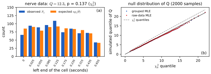
fig_10_s7. Download: PDF · SVGThe book ends the section with a caution: rejecting tells us not to use the model, but not rejecting does not tell us the model is right (the test may lack power), which is an argument for nonparametric methods when they are available. Statistical Methods for Modern Biology fits and tests discrete distributions the same way in Filling the gap 2.3.
10.9 Bibliographic Remarks
p. 169 The most complete reference on testing is Lehmann (1986); see also Chapter 8 of Casella and Berger (2002) and Chapter 9 of Rice (1995). The false discovery rate is due to Benjamini and Hochberg (1995). Some exercises come from Rice (1995). For the asymptotic theory behind Theorems 10.17, 10.22 and 10.29, van der Vaart (1998), Chapters 16 and 17, is the standard modern account.
10.10 Appendix
10.10.1 The Neyman-Pearson Lemma
p. 170 For a simple null against a simple alternative, the most powerful test is known.
Theorem 10.30 (Neyman–Pearson) p. 170
To test \(H_0:\th=\th_0\) against \(H_1:\th=\th_1\), let
\[ T=\frac{L(\th_1)}{L(\th_0)}=\frac{\prod_{i=1}^nf(x_i;\th_1)}{\prod_{i=1}^nf(x_i;\th_0)}. \]If we reject when \(T>k\), with \(k\) chosen so that \(\P_{\th_0}(T>k)=\alpha\), then this test is the most powerful size \(\alpha\) test: among all tests of size \(\alpha\), it maximises \(\beta(\th_1)\).
Filling the gap 10.16: proof of the Neyman–Pearson lemma, and what to do when \(\P_{\th_0}(T>k)=\alpha\) has no solution p. 170
Write \(f_0,f_1\) for the joint densities (or mass functions) of the data under \(\th_0,\th_1\), and describe a test by a function \(\phi(x)\in[0,1]\), the probability of rejecting when \(x\) is observed (a non-randomised test has \(\phi\in\{0,1\}\)). (a) If \(\phi^\ast=1\) where \(f_1>kf_0\) and \(\phi^\ast=0\) where \(f_1<kf_0\), for some \(k\ge0\), then every test \(\phi\) with \(\E_0\phi\le\E_0\phi^\ast\) has \(\E_1\phi\le\E_1\phi^\ast\). (b) For every \(\alpha\in(0,1)\) there are \(k\ge0\) and \(\gamma\in[0,1]\) such that \(\phi^\ast=\I\{T>k\}+\gamma\I\{T=k\}\) has \(\E_0\phi^\ast=\alpha\). (c) In discrete models an exact non-randomised size \(\alpha\) test may not exist; then the best non-randomised level \(\alpha\) tests are of the form \(\I\{T>k\}\) with smaller size.
Proof
(a) For every \(x\), \((\phi^\ast(x)-\phi(x))(f_1(x)-kf_0(x))\ge0\): where \(f_1>kf_0\), \(\phi^\ast=1\ge\phi\); where \(f_1<kf_0\), \(\phi^\ast=0\le\phi\); elsewhere the second factor is 0. Integrating,
\[ \E_1\phi^\ast-\E_1\phi\ \ge\ k\,(\E_0\phi^\ast-\E_0\phi)\ \ge\ 0. \](b) Let \(a(k)=\P_0(T>k)\), with \(T=+\infty\) where \(f_0=0<f_1\) (a set of \(\P_0\)-probability 0). \(a\) is non-increasing and right-continuous, \(a(k)\to0\) as \(k\to\infty\) and \(a(0^-)=\P_0(T\ge0)=1\). Let \(k=\inf\{c:a(c)\le\alpha\}\). Then \(a(k)\le\alpha\le a(k^-)=\P_0(T\ge k)\). If \(\P_0(T=k)=0\), \(a(k)=\alpha\) and \(\gamma=0\) works; otherwise \(\gamma=(\alpha-a(k))/\P_0(T=k)\in[0,1]\). This \(\phi^\ast\) is of the form in (a), so it is most powerful. (c) For \(n=10\) Bernoulli trials, \(p_0=0.5\) against \(p_1=0.7\), \(T\) is increasing in \(S=\sum_iX_i\); \(\P_0(S\ge8)=0.0547\) and \(\P_0(S\ge9)=0.0107\), so \(\P_0(T>k)=0.05\) is impossible: the book's condition has no solution. The randomised test rejects when \(S\ge9\) and with probability \(\gamma=(0.05-0.0107)/\P_0(S=8)=0.893\) when \(S=8\). ∎
The lemma is about one alternative at a time; when the most powerful test is the same for all \(\th_1\) in a one-sided alternative, it is uniformly most powerful, as for Example 10.2 (Filling the gap 10.1). The likelihood ratio statistic of Section 10.6 extends the idea to composite hypotheses, where no optimality theorem of this strength holds. The first-year notes give the same proof (Theorem 6.1) and Statistical Methods for Modern Biology applies it to a coin (Result 6.2).
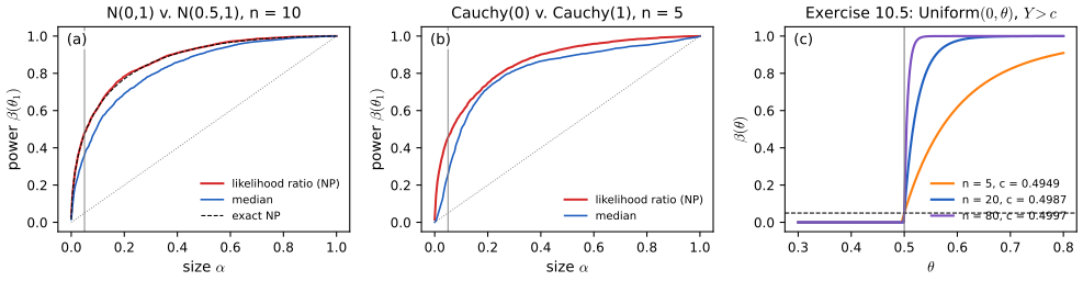
fig_10_s6. Download: PDF · SVG10.10.2 The t-test
p. 170 To test \(H_0:\mu=\mu_0\) for \(\mu=\E(X_i)\) we can use the Wald test; for Normal data and small samples the \(t\)-test is used instead. A random variable has the \(t\) distribution with \(k\) degrees of freedom if its density is
\[ f(t)=\frac{\Gamma\big(\frac{k+1}2\big)}{\sqrt{k\pi}\,\Gamma\big(\frac k2\big)\big(1+\frac{t^2}k\big)^{(k+1)/2}}. \]It tends to the Normal as \(k\to\infty\) and is the Cauchy for \(k=1\). For \(X_1,\dots,X_n\sim N(\mu,\sigma^2)\) with both parameters unknown, let \(T=\sqrt n(\overline X_n-\mu_0)/S_n\), \(S_n^2\) the sample variance. For large \(n\), \(T\approx N(0,1)\) under \(H_0\), but its exact null distribution is \(t_{n-1}\); rejecting when \(|T|>t_{n-1,\alpha/2}\) gives a test of exact size \(\alpha\).
Filling the gap 10.17: why \(T\sim t_{n-1}\) exactly, the limits of the \(t\) density, and the cost of using \(z\) p. 170
(a) If \(Z\sim N(0,1)\) and \(V\sim\chisq{k}\) are independent, \(Z/\sqrt{V/k}\) has the density above. (b) For Normal data, \(\sqrt n(\overline X_n-\mu)/\sigma\sim N(0,1)\) and \((n-1)S_n^2/\sigma^2\sim\chisq{n-1}\) are independent, so \(T\sim t_{n-1}\) under \(H_0\). (c) The \(t_k\) density converges pointwise to \(\phi\) as \(k\to\infty\), and equals the Cauchy density \(1/(\pi(1+t^2))\) for \(k=1\). (d) Using \(z_{\alpha/2}\) with \(S_n\) (the Wald test) has exact size \(2\P(t_{n-1}>z_{\alpha/2})\): 0.122 for \(n=5\), 0.082 for \(n=10\), 0.060 for \(n=30\) at \(\alpha=0.05\).
Proof
(a) Condition on \(V=v\): \(Z/\sqrt{v/k}\) is \(N(0,k/v)\). Integrating against the \(\chisq{k}\) density, the density of the ratio is
\[ \int_0^\infty\sqrt{\frac v{2\pi k}}\,e^{-t^2v/(2k)}\,\frac{v^{k/2-1}e^{-v/2}}{2^{k/2}\Gamma(k/2)}\,\d v=\frac{1}{\sqrt{2\pi k}\,2^{k/2}\Gamma(k/2)}\int_0^\infty v^{(k+1)/2-1}e^{-v(1+t^2/k)/2}\,\d v, \]and the Gamma integral \(\int_0^\infty v^{a-1}e^{-bv}\d v=\Gamma(a)/b^a\) with \(a=(k+1)/2\), \(b=(1+t^2/k)/2\) gives the stated formula after simplification (\[ 2^{(k+1)/2}/(\sqrt{2\pi k}\,2^{k/2})=1/\sqrt{k\pi} \]). (b) This is the Normal-sample theorem, proved in the first-year notes (Theorem 0.9) and in Statistical Methods for Modern Biology (Filling the gap 6.6): an orthogonal change of variables separates \(\overline X_n\) from the residuals. Then \(T=Z/\sqrt{V/(n-1)}\) with \(Z=\sqrt n(\overline X_n-\mu_0)/\sigma\) and \(V=(n-1)S_n^2/\sigma^2\). (c) \((1+t^2/k)^{-(k+1)/2}\to e^{-t^2/2}\), and \(\Gamma((k+1)/2)/\Gamma(k/2)\sim\sqrt{k/2}\) (Stirling), so the constant tends to \(1/\sqrt{2\pi}\); for \(k=1\), \(\Gamma(1)=1\) and \(\Gamma(1/2)=\sqrt\pi\). (d) \(\P(|T|>z_{\alpha/2})\) with \(T\sim t_{n-1}\). ∎
The \(t\) and Cauchy facts are also in Result 2.9 of Chapter 2. The exactness depends on Normality; for non-Normal data the \(t\)-test is only approximately valid, and the permutation test of Section 10.5 is the exact alternative for two samples.
See also: the first-year notes, exact size of the \(t\)-test and the hypothesis test on trial; Statistical Methods for Modern Biology, Result 6.3; Applied Statistical Learning, Filling the gap 13.1.
Notes on the book
Four slips of Chapter 10 are in the author's errata lists; the other points are mine, each with its evidence. Two of them (the permutation p-value and Theorem 10.22) affect conclusions or statements, the rest are small.
Pages 162–163, Section 10.5: the permutation p-value should count ties (\(\ge\), not \(>\))
The book defines the permutation p-value as \(\P_0(T>t_{\rm obs})\) and the Monte Carlo version as \(B^{-1}\sum_j\I(T_j>t_{\rm obs})\). Theorem 10.12, two pages earlier, uses \(\ge\), and only that convention gives a valid test: with "\(>\)" the p-value is 0 with positive probability under \(H_0\) (Filling the gap 10.11(d), Figure 10.S2(b)). The difference matters in both examples. In Example 10.19 the p-value is \(\P_0(T\ge2)=1\), not 4/6. In Example 10.20, enumerating all 252 splits gives \(\P_0(T\ge710)=30/252=0.119\), while \(\P_0(T>710)=12/252=0.048\), which is what the book's simulated 0.045 estimates; with ties counted, gene 1 shows no significant difference at the 5% level, reversing the book's conclusion. The Monte Carlo p-value should be \((1+\#\{T_b\ge t_{\rm obs}\})/(B+1)\). Not in the errata lists.
Page 164, Theorem 10.22: the limit is \(\chi^2_{r-q}\), not \(\chi^2_{r-q,\alpha}\)
The theorem states \(\lambda(x^n)\convd\chisq{r-q,\alpha}\). By the book's own notation (Section 10.3), \(\chisq{k,\alpha}\) is a number, the upper \(\alpha\) quantile; a statistic converges in distribution to the distribution \(\chisq{r-q}\), and the next sentence of the theorem (the p-value \(\P(\chisq{r-q}>\lambda)\)) uses it that way. Not in the errata lists.
Page 150, (10.4): the size should not be called \(\alpha\)
Equation (10.4) reads \(\alpha=\sup_{\th\in\Theta_0}\beta(\th)\), and the next line says a test has level \(\alpha\) if its size is at most \(\alpha\). The left side should be "size". Listed in the author's errata (second printing).
Page 169, Section 10.8 and Theorem 10.29: \(p_i\) should be \(p_j\), and "\(H-0\)" should be \(H_0\)
In the grouped likelihood \(\mathcal Q(\th)=\prod_jp_i(\th)^{N_j}\) the index should be \(j\) throughout, and the statement of Theorem 10.29 prints "Under \(H-0\)". Both listed in the author's errata.
Page 156, Definition 10.11: notation \(X^n\)
\(X^n\) and \(x^n\) are used without definition; they mean \((X_1,\dots,X_n)\) and its observed value \((x_1,\dots,x_n)\). Listed in the author's errata. (The errata also add, for page 151, that \(Z\) denotes a \(N(0,1)\) variable; the printing used for these notes already says so.)
Page 151, Example 10.2: \(N(\mu,\sigma)\) should be \(N(\mu,\sigma^2)\)
The book's convention (Chapter 2) writes the Normal with its variance, and the calculation that follows standardises by \(\sigma/\sqrt n\), treating \(\sigma\) as the standard deviation. Not in the errata lists.
Page 155, Theorem 10.10: the interval must be closed
With the open interval \[ C=(\hth-\hse z_{\alpha/2},\ \hth+\hse z_{\alpha/2}), \] a null value at an endpoint lies outside \(C\) but has \(|W|=z_{\alpha/2}\), which the test does not reject; the equivalence holds with the closed interval (Filling the gap 10.5). This affects only an event of probability zero for continuous data. Not in the errata lists.
Pages 158–159, Example 10.15: \(W=3.77\), and the two bootstrap standard errors
From the summaries of Example 7.15, \(W=20.92/5.55=3.769\) (or \(20.9/\sqrt{5^2+2.4^2}=3.768\)), so 3.77 rather than the printed 3.78; the p-value \(2\Phi(-3.77)=0.00016\) still rounds to 0.0002. The bootstrap standard error of the difference of medians is 7.7 here but 7.42 in Example 8.5 for the same data, presumably two bootstrap runs; the p-value is 0.016 or 0.013, "0.02" either way. Not in the errata lists.
Page 166, proof of Theorem 10.24: sum over the true nulls
The proof bounds \(\P(R)\) by \(\sum_{i=1}^m\P(R_i)=\sum_{i=1}^m\alpha/m\). A false rejection of a false null is impossible, so the sum runs over the \(m_0\) true nulls, and \(\P(R_i)\le\alpha/m\) (with equality only for continuous null p-values); the result is the sharper \(m_0\alpha/m\) (Filling the gap 10.13). The conclusion stands. Not in the errata lists.
10.11 Exercises
All sixteen exercises of Chapter 10 (Wasserman, 2004, pp. 170–173), restated in my own words, with complete solutions (hidden). Computational answers come from the chapter code (functions ex5 to ex12_sim, lrt_exact_size, wald_sd_exact_size, binom_exact_size).
Exercise 10.1. Prove Theorem 10.6.
Solution
See Filling the gap 10.3(a): writing \(W=(\hth-\th_\star)/\hse+(\th_\star-\th_0)/\hse\), the first term is approximately \(N(0,1)\) under \(\th_\star\) and the second approximately the constant \(\delta=(\th_\star-\th_0)/\se\); then \[ \P(W>z_{\alpha/2})\approx1-\Phi(z_{\alpha/2}-\delta) \] and \[ \P(W<-z_{\alpha/2})\approx\Phi(-z_{\alpha/2}-\delta), \] whose sum is (10.6). The approximation is exact for a Normal mean with known variance and is the limit of the power along local alternatives \(\th_0+h/\sqrt n\).
Exercise 10.2. Prove Theorem 10.14.
Solution
See Filling the gap 10.7(a): the p-value is \(\bar F(T)\) with \(\bar F(t)=\P_{\th_0}(T\ge t)=1-F(t)\) for a continuous null cdf \(F\), and \(F(T)\sim\Unif(0,1)\) by the probability integral transform; so \(\P(\text{p-value}\le\alpha)=\alpha\), which is the type I error rate of "reject when the p-value is at most \(\alpha\)".
Exercise 10.3. Prove Theorem 10.10.
Solution
\[ |W|>z_{\alpha/2}\iff|\hth-\th_0|>z_{\alpha/2}\hse\iff\th_0\notin[\hth-z_{\alpha/2}\hse,\hth+z_{\alpha/2}\hse] \] (Filling the gap 10.5, where the boundary case and the general inversion of tests are also treated).
Exercise 10.4. Prove Theorem 10.12.
Solution
See Filling the gap 10.6: with \(G(t)=\sup_{\th\in\Theta_0}\P_\th(T\ge t)\) and tests \(\{T\ge c_\alpha\}\) of size \(\alpha\), the rejection regions are nested, the test rejects at level \(\alpha\) exactly when \(G(t_{\rm obs})\le\alpha\) (up to the boundary), and the infimum of such \(\alpha\) is \(G(t_{\rm obs})\).
Exercise 10.5. \(X_1,\dots,X_n\sim\Unif(0,\th)\) and \(Y=\max_iX_i\). Test \(H_0:\th=1/2\) against \(H_1:\th>1/2\) by rejecting when \(Y>c\) (the Wald test is unsuitable since \(Y\) is not asymptotically Normal). (a) Find the power function. (b) Which \(c\) gives size 0.05? (c) With \(n=20\) and \(Y=0.48\), find the p-value and conclude. (d) The same with \(Y=0.52\).
Solution
(a) \(\P_\th(Y\le y)=(y/\th)^n\) for \(0\le y\le\th\), so \(\beta(\th)=\P_\th(Y>c)=1-(c/\th)^n\) for \(\th>c\) and 0 for \(\th\le c\). (b) Size \(\beta(1/2)=1-(2c)^n=0.05\) gives \(c=\tfrac12(0.95)^{1/n}\); for \(n=20\), \(c=0.4987\). (c) By Theorem 10.12 the p-value is \(\P_{1/2}(Y\ge0.48)=1-(0.96)^{20}=0.558\): no evidence against \(H_0\). (d) \(\P_{1/2}(Y\ge0.52)=0\): under \(H_0\) no observation can exceed 1/2, so the data refute \(H_0\) with certainty (p-value 0). The test is also uniformly most powerful: for any \(\th_1>1/2\) the likelihood ratio \[ L(\th_1)/L(1/2)=(1/2)^n\th_1^{-n}\I\{Y\le\th_1\}/\I\{Y\le1/2\} \] is non-decreasing in \(Y\) (Figure 10.S6(c)).
Exercise 10.6. Of 1919 deaths around Passover (Phillips and King, 1988), 922 occurred in the week before and 997 in the week after. Treating the count before as Binomial\((1919,\th)\), test \(\th=1/2\), interpret the p-value, and give a confidence interval for \(\th\).
Solution
\(\hth=922/1919=0.4805\), \(\hse=\sqrt{\hth(1-\hth)/1919}=0.0114\), \(W=(0.4805-0.5)/0.0114=-1.71\), p-value \(2\Phi(-1.71)=0.087\) (the exact binomial test gives 0.091). This is weak evidence (on the book's scale) that fewer deaths occur just before the holiday than just after, in line with the postponement theory but far from conclusive. The 95% interval is \(0.4805\pm1.96(0.0114)=(0.458,\ 0.503)\): it contains 1/2, and it says that if there is an effect, at most about 4 percentage points of the deaths shift.
Exercise 10.7. Proportions of three-letter words in eight essays by Mark Twain (0.225, 0.262, 0.217, 0.240, 0.230, 0.229, 0.235, 0.217) and ten signed Quintus Curtius Snodgrass (0.209, 0.205, 0.196, 0.210, 0.202, 0.207, 0.224, 0.223, 0.220, 0.201) (Brinegar, 1963). (a) Wald test of equal means with the nonparametric plug-in estimator; p-value and 95% interval for the difference. (b) A permutation test.
Solution
(a) \(\overline x-\overline y=0.2319-0.2097=0.0222\). With the plug-in variances (divisor \(n\)), \(\hse=0.00562\), \(W=3.94\), p-value \(8.0\times10^{-5}\), and the 95% interval is \((0.0112,\ 0.0332)\). (With the \(n-1\) sample variances, \(\hse=0.00599\), \(W=3.70\), p-value 0.0002.) (b) There are \(\binom{18}{8}=43\,758\) splits; exactly 35 give \(|\overline x-\overline y|\ge0.0222\), so the exact permutation p-value is \(35/43\,758=0.0008\) (Figure 10.S4(b)). Both tests find strong evidence that Twain used three-letter words more often than "Snodgrass": the word-length profile argues against Twain's authorship, as Brinegar concluded. The permutation p-value is larger than the Wald one, as expected with eight and ten observations, but the conclusion does not depend on large-sample theory.
Exercise 10.8. \(X_1,\dots,X_n\sim N(\th,1)\); test \(H_0:\th=0\) against \(H_1:\th=1\) by rejecting when \(\overline X_n>c\). (a) Find \(c\) for size \(\alpha\). (b) Find \(\beta(1)\). (c) Show \(\beta(1)\to1\).
Solution
(a) Under \(H_0\), \(\sqrt n\overline X_n\sim N(0,1)\), so \(c=z_\alpha/\sqrt n\). (b) Under \(\th=1\), \(\sqrt n(\overline X_n-1)\sim N(0,1)\), so \[ \beta(1)=\P(\sqrt n(\overline X_n-1)>z_\alpha-\sqrt n)=1-\Phi(z_\alpha-\sqrt n). \] (c) \(z_\alpha-\sqrt n\to-\infty\), so \(\beta(1)\to1\). (By the Neyman–Pearson lemma this test is most powerful; for \(\alpha=0.05\) and \(n=10\), \(\beta(1)=0.9354\).)
Exercise 10.9. Let \(\hth\) be the MLE and \(\hse=\{nI(\hth)\}^{-1/2}\). For the Wald test of \(\th=\th_0\) against \(\th\ne\th_0\) and an alternative \(\th_1>\th_0\), show \(\beta(\th_1)\to1\).
Solution
Under \(\th_1\) and the regularity conditions of Chapter 9, \(\hth\convp\th_1\) and \(\sqrt n(\hth-\th_1)\convd N(0,1/I(\th_1))\), and \(I(\hth)\convp I(\th_1)\) if \(I\) is continuous. Then \(\sqrt{nI(\hth)}(\hth-\th_1)\) is bounded in probability while \(\sqrt{nI(\hth)}(\th_1-\th_0)\to\infty\) in probability, so \(W=(\hth-\th_0)/\hse\to\infty\) in probability and \(\P_{\th_1}(|W|>z_{\alpha/2})\to1\). The details are in Filling the gap 10.3(b).
Exercise 10.10. Deaths of elderly Chinese and Jewish women in the two weeks before and after the Chinese Harvest Moon Festival (Phillips and Smith, 1990): Chinese 55, 33, 70, 49 and Jewish 141, 145, 139, 161 in weeks \(-2,-1,1,2\). Compare the two mortality patterns.
Solution
Treat the table as two independent multinomials and test whether they share the same week distribution (homogeneity). Expected counts are row total times column total over 793; Pearson's statistic is \(X^2=12.42\) on \((2-1)(4-1)=3\) degrees of freedom, p-value 0.006 (the likelihood ratio statistic is 12.53, p-value 0.006). The patterns differ. The difference sits around the festival: Chinese deaths dip in the week before (33, against about 46 expected under a common pattern) and peak in the week after (70), while Jewish deaths are flat. For the Chinese women alone, the share of deaths in the two weeks before is \(88/207=0.425\), Wald \(W=-2.18\), p-value 0.029; for the Jewish women it is \(286/586=0.488\), p-value 0.56. This is the postponement pattern of Exercise 10.6, appearing in the group for which the festival matters, with the Jewish women serving as a control. (Collapsing the table to before/after loses the week detail: \(X^2=2.43\) on 1 degree of freedom, p-value 0.12.)
Exercise 10.11. A double-blind trial of drugs against postoperative nausea (Beecher, 1959): placebo 45 of 80 patients with nausea, chlorpromazine 26 of 75, dimenhydrinate 52 of 85, pentobarbital 100 mg 35 of 67, pentobarbital 150 mg 37 of 85. (a) Test each drug against placebo at 5% and report odds ratios. (b) Adjust for multiple testing with Bonferroni and with the FDR method.
Solution
(a) Placebo rate \(45/80=0.5625\). For each drug, the Wald test of Example 10.7 for \(p_{\rm drug}-p_{\rm placebo}\) and the odds ratio \[ \{\hat p_1/(1-\hat p_1)\}/\{\hat p_0/(1-\hat p_0)\} \] with a 95% interval from \(\hse(\log OR)=\sqrt{1/a+1/b+1/c+1/d}\):
drug rate \(W\) p-value odds ratio (95% interval) chlorpromazine 0.347 −2.76 0.0057 0.41 (0.22, 0.79) dimenhydrinate 0.612 0.64 0.52 1.23 (0.66, 2.28) pentobarbital 100 mg 0.522 −0.49 0.63 0.85 (0.44, 1.63) pentobarbital 150 mg 0.435 −1.65 0.10 0.60 (0.32, 1.11) At 5%, only chlorpromazine differs from placebo: it reduces the odds of nausea by about 60%. Pentobarbital 150 mg points the same way but is not significant. (b) Bonferroni with \(m=4\) rejects when \(p<0.0125\): chlorpromazine only. BH: the ordered p-values 0.0057, 0.0996, 0.52, 0.63 against \(0.0125i\): only the first is under the line, so BH also rejects chlorpromazine only (and so does BH with \(C_4=2.083\)). The conclusion is robust to the adjustment.
Exercise 10.12. \(X_1,\dots,X_n\sim\Pois(\lambda)\). (a) Find the size \(\alpha\) Wald test of \(\lambda=\lambda_0\) against \(\lambda\ne\lambda_0\). (b) With \(\lambda_0=1\), \(n=20\), \(\alpha=0.05\), simulate many data sets under \(H_0\) and count how often the test rejects.
Solution
(a) The MLE is \(\hat\lambda=\overline X_n\), with \(\V(\hat\lambda)=\lambda/n\) and \(\hse=\sqrt{\hat\lambda/n}\) (also \(\{nI(\hat\lambda)\}^{-1/2}\), since \(I(\lambda)=1/\lambda\)). Reject when \(|W|>z_{\alpha/2}\), \(W=(\hat\lambda-\lambda_0)/\sqrt{\hat\lambda/n}\) (or \(\sqrt{\lambda_0/n}\) in the denominator, Remark 10.5). (b) With 10,000 simulated data sets the test rejected 5.23% of the time. Since \(S=n\hat\lambda\sim\Pois(n\lambda_0)\), the exact size is a Poisson sum: 0.0525 at \(n=20\), close to 0.05. It oscillates with \(n\) (0.074 at \(n=10\), 0.051 at \(n=50\), 0.055 at \(n=100\); Figure 10.S1(c)).
▶ DemoExercise 10.12: Poisson, \(\lambda_0=1\), \(n=20\)10,000 simulations, 5.23% rejected; exact size 0.0525.Exercise 10.13. \(X_1,\dots,X_n\sim N(\mu,\sigma^2)\). Construct the likelihood ratio test of \(\mu=\mu_0\) against \(\mu\ne\mu_0\) and compare it with the Wald test.
Solution
The log-likelihood is \[ -\frac n2\log\sigma^2-\frac1{2\sigma^2}\sum_i(x_i-\mu)^2. \] Unrestricted: \(\hat\mu=\overline x\), \(\hat\sigma^2=n^{-1}\sum_i(x_i-\overline x)^2\). Restricted: \[ \tilde\sigma^2=n^{-1}\sum_i(x_i-\mu_0)^2=\hat\sigma^2+(\overline x-\mu_0)^2. \] Both maximised log-likelihoods equal \(-\frac n2\log(\cdot)-\frac n2\), so
\[ \lambda=n\log\frac{\tilde\sigma^2}{\hat\sigma^2}=n\log\Big(1+\frac{(\overline x-\mu_0)^2}{\hat\sigma^2}\Big)=n\log\Big(1+\frac{T^2}{n-1}\Big), \]with \(T=\sqrt n(\overline x-\mu_0)/S_n\) the \(t\) statistic. The Wald statistic with the MLE standard error is \(W=\sqrt n(\overline x-\mu_0)/\hat\sigma\), so \(W^2=nT^2/(n-1)\) and \[ \lambda=n\log(1+W^2/n)=W^2-W^4/(2n)+\dots. \] All three statistics are increasing functions of \(|T|\): the tests differ only in their cut-offs. Calibrated with \(\chisq{1,0.05}\), the likelihood ratio test has exact size 0.098 at \(n=5\), 0.070 at \(n=10\), 0.054 at \(n=50\); the Wald test with \(z_{0.025}\) has 0.154, 0.096 and 0.058; the \(t\)-test is exact. For Normal data, use the \(t\) cut-off; asymptotically all three agree (Exercise 10.16).
Exercise 10.14. \(X_1,\dots,X_n\sim N(\mu,\sigma^2)\). Construct the likelihood ratio test of \(\sigma=\sigma_0\) against \(\sigma\ne\sigma_0\) and compare it with the Wald test.
Solution
Under both hypotheses \(\hat\mu=\overline x\). Unrestricted \(\hat\sigma^2\) as above; restricted \(\sigma^2=\sigma_0^2\). With \(s=\hat\sigma^2/\sigma_0^2\),
\[ \lambda=2\Big[-\frac n2\log\hat\sigma^2-\frac n2+\frac n2\log\sigma_0^2+\frac{n\hat\sigma^2}{2\sigma_0^2}\Big]=n\,(s-1-\log s). \]Since \[ ns=\sum_i(x_i-\overline x)^2/\sigma_0^2\sim\chisq{n-1} \] under \(H_0\), the exact size of any rule based on \(s\) is a \(\chi^2\) probability. The Wald test uses \(\hat\sigma\) with \(\hse=\hat\sigma/\sqrt{2n}\) (the Fisher information for \(\sigma\) is \(2/\sigma^2\) per observation): \(W=\sqrt{2n}(\hat\sigma-\sigma_0)/\hat\sigma\). Calibrated asymptotically, the exact sizes at \(\alpha=0.05\) are: likelihood ratio 0.106 (\(n=5\)), 0.074 (\(n=10\)), 0.054 (\(n=50\)); Wald 0.247, 0.152, 0.071. The Wald test is poor here because \(\hat\sigma\) is skewed and its standard error is estimated by itself; the likelihood ratio test respects the skewness (it is invariant to reparametrising by \(\sigma^2\) or \(\log\sigma\), the Wald test is not). An exact test uses the \(\chisq{n-1}\) quantiles of \(ns\) directly.
Exercise 10.15. \(X\sim\Bin(n,p)\). Construct the likelihood ratio test of \(p=p_0\) against \(p\ne p_0\) and compare it with the Wald test.
Solution
With \(\hat p=X/n\),
\[ \lambda=2\Big[X\log\frac{\hat p}{p_0}+(n-X)\log\frac{1-\hat p}{1-p_0}\Big] \](with \(0\log0=0\)); reject when \(\lambda>\chisq{1,\alpha}\). The Wald test uses \(W=(\hat p-p_0)/\sqrt{\hat p(1-\hat p)/n}\). Both are functions of \(X\), so their exact sizes are binomial sums. For \(p_0=0.5\) both statistics are symmetric and increasing in \(|X-n/2|\), so the two tests coincide (size 0.041 at \(n=20\)). For \(p_0=0.1\) they differ: at \(n=20\) the sizes are 0.124 (Wald) and 0.133 (likelihood ratio); at \(n=50\), 0.121 and 0.058; at \(n=100\), 0.068 and 0.044. Away from \(p_0=1/2\) the likelihood ratio test is usually much closer to its nominal level, because the Wald standard error collapses when \(\hat p\) is near 0 (Filling the gap 10.2).
Exercise 10.16. For a scalar \(\th\), show that the Wald statistic \(W\) and the likelihood ratio statistic \(\lambda\) for \(\th=\th_0\) satisfy \(W^2/\lambda\convp1\) under \(H_0\). Hint: expand the log-likelihood to show
\[ \lambda\approx\big(\sqrt n(\hth-\th_0)\big)^2\big(-n^{-1}\ell''(\hth)\big). \]Solution
Assume the regularity conditions of Chapter 9 and use \(\hse=\{nI(\hth)\}^{-1/2}\), so \(W^2=n(\hth-\th_0)^2I(\hth)\). Expand \(\ell(\th_0)\) around \(\hth\), where \(\ell'(\hth)=0\): \[ \ell(\th_0)=\ell(\hth)+\frac12\ell''(\bar\th)(\th_0-\hth)^2 \] for some \(\bar\th\) between \(\th_0\) and \(\hth\). Hence \[ \lambda=2[\ell(\hth)-\ell(\th_0)]=n(\hth-\th_0)^2\big(-n^{-1}\ell''(\bar\th)\big). \] On the event \(\hth\ne\th_0\) (probability tending to 1),
\[ \frac{W^2}\lambda=\frac{I(\hth)}{-n^{-1}\ell''(\bar\th)}. \]Under \(H_0\), \(\hth\convp\th_0\) and so \(\bar\th\convp\th_0\); \(I(\hth)\convp I(\th_0)\) by continuity; and \(-n^{-1}\ell''(\bar\th)\convp I(\th_0)\) by the law of large numbers for \(-n^{-1}\ell''(\th_0)\) together with the domination of the third derivative, which bounds \(|n^{-1}\ell''(\bar\th)-n^{-1}\ell''(\th_0)|\) by a constant times \(|\bar\th-\th_0|\). The ratio tends to \(I(\th_0)/I(\th_0)=1\) in probability. (With \(\hse=\{-\ell''(\hth)\}^{-1/2}\) instead, the same argument applies.) Exercise 10.13 shows it concretely: \(\lambda=n\log(1+W^2/n)\) and \(W^2/\lambda\to1\) because \(W^2/n\convp0\).
Demonstrations for this chapter
Each demonstration runs in the browser and links back to these notes. The ▶ Demo boxes above open them already set to the case under discussion.
| Demonstration | What you can see | Sections and results |
|---|---|---|
| The power function of the Wald test | Exact power against the approximation (10.6) for a Normal mean, a Bernoulli probability and a Poisson mean; the exact size against \(n\); estimated or null standard error; one- or two-sided; a seeded simulation. Presets: 1 Example 10.2; 2 Theorem 10.6; 3 Bernoulli lattice; 4 Exercise 10.12; 5 Remark 10.5. | Example 10.2, 10.1; Filling the gaps 10.2, 10.3 |
| The Neyman–Pearson lemma | Simulated log likelihood ratios under both hypotheses with the critical value, and ROC curves of the likelihood ratio test and a competitor, for Normal, Laplace and Cauchy locations and a Normal scale. Presets: 1 Normal mean; 2 Laplace; 3 Cauchy; 4 Normal scale; 5 one Cauchy observation. | 10.10.1; Theorem 10.30, Filling the gap 10.16 |
| The permutation test is exact | The exact permutation distribution of three statistics for the book's small data sets, p-values with and without ties, a Monte Carlo version and the Wald p-value; and the size under \(H_0\) of the Wald, pooled \(t\) and permutation tests in small samples. Presets: 1 Example 10.19; 2 Example 10.20; 3 Exercise 10.7; 4 size, Normal data; 5 unequal spreads. | 10.5; Filling the gap 10.11; Exercise 10.7 |
Related demonstrations in the companion courses: the first-year hypothesis test on trial, power and sample size and tests and intervals; in Statistical Methods for Modern Biology, the t-test and permutation test, Pearson's statistic and the FDR demos; in Applied Statistical Learning, the Benjamini–Hochberg demo. In this course, the Chapter 1 base-rate demo is the right picture for P(H0 | reject). The Python code that produces every figure of this page is code/ch10_hypothesis_testing.py (see the code index); the data of the permutation demo are in data/ch10-permutation.json.
References
- Wasserman, L. (2004). All of Statistics: A Concise Course in Statistical Inference. Springer, New York. Chapter 10, pp. 149–173. www.stat.cmu.edu/~larry/all-of-statistics.
- Beecher, H. K. (1959). Measurement of Subjective Responses: Quantitative Effects of Drugs. Oxford University Press, New York.
- Benjamini, Y. and Hochberg, Y. (1995). Controlling the false discovery rate: a practical and powerful approach to multiple testing. Journal of the Royal Statistical Society, Series B, 57(1), 289–300.
- Benjamini, Y. and Yekutieli, D. (2001). The control of the false discovery rate in multiple testing under dependency. The Annals of Statistics, 29(4), 1165–1188.
- Brinegar, C. S. (1963). Mark Twain and the Quintus Curtius Snodgrass letters: a statistical test of authorship. Journal of the American Statistical Association, 58(301), 85–96.
- Casella, G. and Berger, R. L. (2002). Statistical Inference, 2nd edition. Duxbury, Pacific Grove.
- Chernoff, H. and Lehmann, E. L. (1954). The use of maximum likelihood estimates in \(\chi^2\) tests for goodness of fit. The Annals of Mathematical Statistics, 25(3), 579–586.
- Cox, D. R. and Lewis, P. A. W. (1966). The Statistical Analysis of Series of Events. Methuen, London. (The nerve data.)
- Efron, B., Tibshirani, R., Storey, J. D. and Tusher, V. (2001). Empirical Bayes analysis of a microarray experiment. Journal of the American Statistical Association, 96(456), 1151–1160.
- Fisher, R. A. (1936). Has Mendel's work been rediscovered? Annals of Science, 1(2), 115–137.
- Holm, S. (1979). A simple sequentially rejective multiple test procedure. Scandinavian Journal of Statistics, 6(2), 65–70.
- Lehmann, E. L. (1986). Testing Statistical Hypotheses, 2nd edition. Wiley, New York.
- Neyman, J. and Pearson, E. S. (1933). On the problem of the most efficient tests of statistical hypotheses. Philosophical Transactions of the Royal Society of London, Series A, 231, 289–337.
- Pearson, K. (1900). On the criterion that a given system of deviations from the probable in the case of a correlated system of variables is such that it can be reasonably supposed to have arisen from random sampling. Philosophical Magazine, Series 5, 50(302), 157–175.
- Phillips, D. P. and King, E. W. (1988). Death takes a holiday: mortality surrounding major social occasions. The Lancet, 332(8613), 728–732.
- Phillips, D. P. and Smith, D. G. (1990). Postponement of death until symbolically meaningful occasions. Journal of the American Medical Association, 263(14), 1947–1951.
- Rice, J. A. (1995). Mathematical Statistics and Data Analysis, 2nd edition. Duxbury, Belmont.
- Scott, D. W., Gotto, A. M., Cole, J. S. and Gorry, G. A. (1978). Plasma lipids as collateral risk factors in coronary artery disease: a study of 371 males with chest pain. Journal of Chronic Diseases, 31(5), 337–345.
- van der Vaart, A. W. (1998). Asymptotic Statistics. Cambridge University Press, Cambridge.
- Wald, A. (1943). Tests of statistical hypotheses concerning several parameters when the number of observations is large. Transactions of the American Mathematical Society, 54(3), 426–482.
- Wilks, S. S. (1938). The large-sample distribution of the likelihood ratio for testing composite hypotheses. The Annals of Mathematical Statistics, 9(1), 60–62.
The numerical statements in the text (the power and size calculations, the Mendel, cholesterol and permutation examples, the multiple-testing examples and simulations, the goodness-of-fit example, the exact sizes of the likelihood ratio and Wald tests, and the solutions of the exercises) were confirmed numerically.