Additive Models, Trees, and Related Methods
Every method in this chapter beats the curse of dimensionality by assuming a structure for the regression function. A generalised additive model writes it as a sum of smooth functions of one input each and fits all of them at once by cycling a one-dimensional smoother over the inputs (backfitting). A tree cuts the input space into boxes by a greedy sequence of binary splits, grows a large tree and prunes it back by a cost-complexity criterion whose solutions form a single nested sequence. PRIM looks for boxes with a high mean by peeling the data away slowly; MARS builds a regression surface from products of hinge functions, a tree that can also add; and a hierarchical mixture of experts replaces the tree's hard splits by soft, probabilistic ones fitted by EM. The chapter ends with how these methods, and others, cope with missing inputs.
Ch. 1 Introduction Ch. 2 Supervised learning Ch. 3 Linear regression Ch. 4 Linear classification Ch. 5 Basis expansions Ch. 6 Kernel smoothing Ch. 7 Model assessment Ch. 8 Inference and averaging Ch. 9 Additive models and trees Ch. 10 Boosting Ch. 11 Neural networks Ch. 12 SVMs Ch. 13 Nearest neighbours Ch. 14 Unsupervised learning Ch. 15 Random forests Ch. 16 Ensembles Ch. 17 Graphical models Ch. 18 High-dimensional problems
How to read these notes
They follow the book. Sections carry the book's numbers (9.1, 9.1.1, ...) and every displayed equation that appears in the book carries the book's own equation number, e.g. \((9.7)\), so you can read these notes next to the book. Equations without a number are steps that the book skips.
Filling the gaps. Wherever the book says that something "can be shown", leaves it to an exercise, or states a property without proof, an orange Filling the gap box or a proof gives the full argument. Proofs and derivations start hidden: open one with its bar, or use the button below.
Figures and demonstrations. Every figure of the chapter that is computed from data or a model is reproduced from scratch by the Python code; Figures 9.10 and 9.13 are schematic diagrams and are not redrawn. Four supplementary figures (9.S1–9.S4) illustrate the exercises and Section 9.5. The ▶ Demo boxes open an interactive demonstration already set to the case being discussed.
Main reference
T. Hastie, R. Tibshirani and J. Friedman, The Elements of Statistical Learning: Data Mining, Inference, and Prediction, 2nd edition, Springer (2009), Chapter 9, pages 295–336 (book website, with the data sets: hastie.su.domains/ElemStatLearn). Section, equation, figure and exercise numbers below refer to this book. Further reading is listed in the references.
The explanations, derivations, figures and code are my own; equations are cited by their numbers in the book.
Companion courses
Parts of this chapter also appear in the two companion courses on this site. The overlapping material is:
- Sections 9.2.2–9.2.3 (growing and pruning trees, node impurities): Bayesian and Probabilistic Machine Learning, Section 14.4, with Definition 14.2, Result 14.9 (optimal pruning for one \(\alpha\) by dynamic programming) and Result 14.10 (why impurities beat the misclassification rate).
- Section 9.5 (mixtures of experts and EM): Bayesian and Probabilistic Machine Learning, Section 14.5, especially Section 14.5.3, and the general theory of EM in Section 9.4.
- Section 9.1.1 (the roughness penalty of (9.7) as a quadratic regulariser) and Section 9.2.4 (averaging unstable trees): Foundations of Deep Learning, Section 9.2.2 (generalised weight decay) and Section 9.6 (model averaging).
- Section 9.1.2 (local scoring as Newton–Raphson): Bayesian and Probabilistic Machine Learning, Section 4.3.3 (iterative reweighted least squares) and, in this course, Result 5.10 (penalised logistic regression as iterated weighted smoothing).
Where a proof there is the same, these notes state the result, sketch the argument and link to it. New here: the existence of the additive cubic-spline solution of (9.7), backfitting as Gauss–Seidel and why it converges, the weakest-link sequence and the proof that it contains every optimal subtree, the ordering trick for categorical inputs, the area under the ROC curve as a Mann–Whitney statistic, PRIM, MARS with its fast knot search, EM for hierarchical mixtures of experts, the ignorability of data missing at random, and three corrections to the book (Table 9.1, Figure 9.5 and Exercise 9.1).
The chapter at a glance
- 9.1 The penalised criterion (9.7) is minimised by an additive cubic spline (Result 9.1); backfitting is block Gauss–Seidel on the normal equations and, for smoothing splines, block coordinate descent on (9.7), so it converges (Result 9.2), slowly when inputs are correlated (Filling the gap 9.2). Local scoring is Newton–Raphson with a weighted backfit inside (Result 9.3). On the spam data the additive logistic model has a test error of 5.5% (84 of 1536), not the 5.3% of the book's text (note).
- 9.2 The best constant in a box is the mean, and one pass over the sorted values finds the best split (Result 9.4). Each \(C_\alpha\) has a unique smallest minimising subtree, these subtrees are nested, and weakest-link pruning lists all of them (Results 9.5–9.6). Gini and entropy reward any split that changes the class proportions (Result 9.7); with two classes the best split of a categorical input is found by ordering its levels (Result 9.8). The area under an ROC curve is a Mann–Whitney statistic (Result 9.9).
- 9.3 PRIM peels a box slowly (Algorithm 9.3); with \(\alpha=0.1\) it can make 29 peels where a tree of 128 points can make 6 splits (Filling the gap 9.11).
- 9.4 MARS adds products of reflected pairs \((x-t)_+,(t-x)_+\); every knot of an input is scored in one pass (Result 9.10), terms are deleted by the cheapest increase of RSS (Result 9.11) and GCV (9.20) picks the size. With step functions and one more rule MARS becomes CART (Result 9.12).
- 9.5–9.6 A hierarchical mixture of experts is fitted by EM with weighted regressions in the M-step (Result 9.13). Under missingness at random the mechanism can be ignored in likelihood inference (Result 9.14), but the complete cases can still be biased.
Notation. Training data \((x_i,y_i)\), \(i=1,\dots,N\), with \(x_i=(x_{i1},\dots,x_{ip})\). Bold lower-case letters are \(N\)-vectors of values at the training points, e.g. \(\bf_j=(f_j(x_{1j}),\dots,f_j(x_{Nj}))^\T\); \(\bone\) is the vector of ones. A linear smoother of one input is an \(N\times N\) matrix \(\bS_j\) acting on such vectors. For trees, \(R(t)\) is the cost of node \(t\) as a leaf (its \(N_tQ_t\)), \(T_t\) the branch below \(t\) and \(|T|\) the number of leaves of \(T\).
Prerequisites. Smoothing splines and their smoother matrices (Chapter 5, Section 5.4), logistic regression and IRLS (Section 4.4), the EM algorithm (Section 8.5) and cross-validation (Section 7.10).
9.1 Generalized Additive Models
pp. 295–297 A linear model is easy to read but assumes that each input acts linearly. A generalised additive model keeps the reading, "the effect of \(X_j\) with the others held fixed", but lets each effect be an arbitrary smooth function.
Definition 9.1 (generalised additive models) pp. 295–297, (9.1)–(9.5)
In regression, an additive model has
\[ \E(Y\given X_1,X_2,\dots,X_p)=\alpha+f_1(X_1)+f_2(X_2)+\cdots+f_p(X_p), \tag{9.1} \]with unspecified smooth functions \(f_j\). For a binary response with \(\mu(X)=\Pr(Y=1\given X)\), linear logistic regression
\[ \log\Big(\frac{\mu(X)}{1-\mu(X)}\Big)=\alpha+\beta_1X_1+\cdots+\beta_pX_p \tag{9.2} \]becomes the additive logistic regression model
\[ \log\Big(\frac{\mu(X)}{1-\mu(X)}\Big)=\alpha+f_1(X_1)+\cdots+f_p(X_p). \tag{9.3} \]In general a generalised additive model (GAM) relates the conditional mean \(\mu(X)\) to an additive predictor through a link function \(g\):
\[ g[\mu(X)]=\alpha+f_1(X_1)+\cdots+f_p(X_p). \tag{9.4} \]The classical links are the identity (Gaussian responses), the logit \(\log\{\mu/(1-\mu)\}\) or the probit \(\Phi^{-1}(\mu)\) (binomial) and the log (Poisson counts). Terms may also be linear (\(X^\T\beta\)), factors (\(\alpha_k\) for level \(k\) of a qualitative input), separate curves for each level of a factor (\(g_k(Z)\)), or functions of two inputs (\(g(Z,W)\)); a time series can be decomposed as
\[ Y_t=S_t+T_t+\varepsilon_t \tag{9.5} \]into a seasonal component, a trend and an error.
Each \(\hf_j\) shows the shape of the effect of \(X_j\), adjusted for all the other inputs. The functions are not modelled by a fixed basis (that would make (9.1) a linear model in the basis, Chapter 5); they are estimated with a scatterplot smoother, and an algorithm, backfitting, fits all \(p\) of them together.
9.1.1 Fitting Additive Models
pp. 297–299 Take the additive model
\[ Y=\alpha+\sum_{j=1}^pf_j(X_j)+\varepsilon, \tag{9.6} \]with \(\E\varepsilon=0\), and fit it by minimising the penalised residual sum of squares
\[ \PRSS(\alpha,f_1,f_2,\dots,f_p)=\sum_{i=1}^N\Big(y_i-\alpha-\sum_{j=1}^pf_j(x_{ij})\Big)^2+\sum_{j=1}^p\lambda_j\int f_j''(t_j)^2\,\d t_j, \tag{9.7} \]with \(\lambda_j\ge0\), over functions with square-integrable second derivatives. For \(p=1\) this is the smoothing-spline problem of Result 5.5.
See also (companion course): Foundations of Deep Learning, Section 9.2.2: the roughness penalty in (9.7) is a quadratic regulariser \(\lambda_j\bf_j^\T\bK_j\bf_j\) of the kind studied there.
Result 9.1 (the minimiser of (9.7) is an additive cubic spline) pp. 297–298
Let all \(\lambda_j>0\). (a) Any minimiser of (9.7) has each \(f_j\) a natural cubic spline with knots at the distinct values of \(x_{1j},\dots,x_{Nj}\). (b) Adding a constant \(c_j\) to \(f_j\) and subtracting it from \(\alpha\) leaves (9.7) unchanged, so impose \(\sum_{i=1}^Nf_j(x_{ij})=0\) for every \(j\); then \(\hat\alpha=\bar y\). (c) If moreover the \(N\times p\) input matrix with entries \(x_{ij}\), centred column by column, has full column rank, the minimiser is unique. (d) Without full rank the fitted vector \(\sum_j\hat\bf_j\) is still unique and two minimisers can differ only by linear functions \(\sum_jb_j(x_j-\bar x_j)\) that vanish at every \(x_i\): the nonlinear parts are always determined.
Proof
(a) Fix any candidate \((\alpha,f_1,\dots,f_p)\) and one index \(j\). Let \(g_j\) be the natural cubic spline that interpolates \(f_j\) at the distinct values \(t_1\lt\dots\lt t_n\) of the \(x_{ij}\) (it exists and is unique for \(n\ge2\)). Replacing \(f_j\) by \(g_j\) changes no fitted value, so the sum of squares in (9.7) is unchanged, while \(\int g_j''^2\le\int f_j''^2\) with equality only if \(f_j=g_j\) (the minimum-curvature property of the natural cubic interpolant; Result 5.5, which is Exercise 5.7). So a minimiser must have every \(f_j\) a natural cubic spline with those knots; the problem becomes finite dimensional: \(f_j=\mathbf N_j\theta_j\) and
\[ \PRSS=\Big\|\by-\alpha\bone-\sum_j\bf_j\Big\|^2+\sum_j\lambda_j\bf_j^\T\bK_j\bf_j, \]where \(\bf_j\) is the vector of values at the data and \(\bK_j\) is the penalty matrix of Section 5.4.1 (expanded to the \(N\) observations, tied values sharing a row). (b) The penalty does not see constants. With every \(\bone^\T\bf_j=0\), the derivative of PRSS in \(\alpha\) is \(-2\bone^\T(\by-\alpha\bone-\sum_j\bf_j)=-2(\bone^\T\by-N\alpha)\), so \(\hat\alpha=\bar y\). (c) PRSS is a convex quadratic in \((\bf_1,\dots,\bf_p)\); it is strictly convex unless there is a direction \(\mathbf d=(\mathbf d_1,\dots,\mathbf d_p)\ne\bzero\) along which it is flat, which needs \(\sum_j\mathbf d_j=\bzero\) and \(\mathbf d_j^\T\bK_j\mathbf d_j=0\) for all \(j\). The null space of \(\bK_j\) consists of the values of linear functions of \(x_j\), so \(\mathbf d_j=a_j\bone+b_j\bx_j\); the centring constraint gives \(\mathbf d_j=b_j(\bx_j-\bar x_j\bone)\); and \(\sum_jb_j(\bx_j-\bar x_j\bone)=\bzero\) with full column rank forces every \(b_j=0\). A strictly convex function has at most one minimiser, and one exists because the quadratic is bounded below. (d) In general the set of minimisers of a convex quadratic is an affine set \(\hat{\mathbf f}+\mathcal D\), \(\mathcal D\) the flat directions just described: they change no fitted value (\(\sum_j\mathbf d_j=\bzero\)) and only the linear parts \(b_j\) of the terms (Buja, Hastie and Tibshirani, 1989). ∎
Algorithm 9.1 (the backfitting algorithm for additive models) p. 298
- Initialise: \(\hat\alpha=\frac1N\sum_1^Ny_i\), \(\hf_j\equiv0\) for all \(i,j\).
- Cycle over \(j=1,2,\dots,p,\dots,1,2,\dots,p,\dots\): \[ \hf_j\leftarrow\mathcal S_j\Big[\Big\{y_i-\hat\alpha-\sum_{k\ne j}\hf_k(x_{ik})\Big\}_1^N\Big],\qquad \hf_j\leftarrow\hf_j-\frac1N\sum_{i=1}^N\hf_j(x_{ij}), \] until the functions \(\hf_j\) change less than a prespecified threshold.
Here \(\mathcal S_j\) is a scatterplot smoother of the partial residuals against \(x_{ij}\): a cubic smoothing spline with parameter \(\lambda_j\), or any other smoother (local polynomial and kernel smoothers; polynomial, piecewise-constant, regression-spline or Fourier fits; surface smoothers for interactions; periodic smoothers for seasonal terms). At the data, a linear smoother is a matrix \(\bS_j\); the degrees of freedom of term \(j\) are taken to be \(\df_j=\Tr(\bS_j)-1\).
Why "\(-1\)": every smoother of interest reproduces constants, so \(\Tr\bS_j\) counts the constant once; in the additive model the constant is the single shared \(\alpha\), and each term only adds its non-constant part. The second line of step 2 removes any mean the smoother has put into \(\hf_j\); Exercise 9.1 shows when it is redundant.
Result 9.2 (backfitting is Gauss–Seidel, and it converges; Exercise 9.2) p. 299
Let the \(\bS_j\) be linear smoothers and centre \(\by\) (so \(\hat\alpha\) drops out). (a) The fixed points of backfitting are the solutions of the normal equations
\[ \begin{pmatrix}\bI&\bS_1&\bS_1&\cdots&\bS_1\\\bS_2&\bI&\bS_2&\cdots&\bS_2\\\vdots&&\ddots&&\vdots\\\bS_p&\bS_p&\bS_p&\cdots&\bI\end{pmatrix}\begin{pmatrix}\bf_1\\\bf_2\\\vdots\\\bf_p\end{pmatrix}=\begin{pmatrix}\bS_1\by\\\bS_2\by\\\vdots\\\bS_p\by\end{pmatrix}, \tag{9.33} \]and one cycle of Algorithm 9.1 (without the centring step) is one sweep of block Gauss–Seidel on (9.33). (b) For cubic smoothing splines, \(\bS_j=(\bI+\lambda_j\bK_j)^{-1}\), the update of \(\bf_j\) is the exact minimiser of PRSS (9.7) over \(\bf_j\) with the others fixed, so backfitting is block coordinate descent on a convex quadratic: PRSS never increases. (c) If the minimiser is unique (Result 9.1(c)), the iterates converge to it from any starting values, linearly: \(\|\bf^{(k)}-\hat\bf\|\le C\rho^k\) with \(\rho\lt1\).
Proof
(a) Block row \(j\) of (9.33) reads \(\bf_j+\bS_j\sum_{k\ne j}\bf_k=\bS_j\by\), i.e. \(\bf_j=\bS_j(\by-\sum_{k\ne j}\bf_k)\). Block Gauss–Seidel solves block row \(j\) for \(\bf_j\) with the other blocks at their latest values, for \(j=1,\dots,p\) in turn: exactly the update of Algorithm 9.1, with the partial residual built from the already updated \(\bf_1,\dots,\bf_{j-1}\) and the old \(\bf_{j+1},\dots,\bf_p\). A fixed point satisfies every block row, and conversely.
(b) As a function of \(\bf_j\) alone, with \(\br_j=\by-\sum_{k\ne j}\bf_k\), PRSS is \(\|\br_j-\bf_j\|^2+\lambda_j\bf_j^\T\bK_j\bf_j+\text{const}\), a strictly convex quadratic whose gradient \(-2(\br_j-\bf_j)+2\lambda_j\bK_j\bf_j\) vanishes at \(\bf_j=(\bI+\lambda_j\bK_j)^{-1}\br_j=\bS_j\br_j\). So each update minimises PRSS exactly over one block. Multiplying block row \(j\) of (9.33) by \(\bS_j^{-1}=\bI+\lambda_j\bK_j\) turns the system into \(\bH\bf=(\by^\T,\dots,\by^\T)^\T\) with the symmetric matrix \(\bH\) that has \(\bI+\lambda_j\bK_j\) on the diagonal blocks and \(\bI\) off the diagonal; \(\bH\) is twice the Hessian of PRSS, \(\bH=\mathbf J^\T\mathbf J+\diag(\lambda_j\bK_j)\) with \(\mathbf J=(\bI,\dots,\bI)\), positive semi-definite.
(c) Write \(P(\bf)=\tfrac12\bf^\T\bH\bf-\mathbf c^\T\bf\) (PRSS up to a factor and a constant). Uniqueness means \(\bH\) is positive definite on the centred functions; let \(\mu_{\min}>0\) be its smallest eigenvalue there. Exact minimisation over block \(j\) changes \(\bf_j\) by \(\Delta_j\) and lowers \(P\) by exactly \(\tfrac12\Delta_j^\T\bH_{jj}\Delta_j\ge\tfrac12\|\Delta_j\|^2\) (expand \(P\) around the new point, where the block gradient is zero; \(\bH_{jj}=\bI+\lambda_j\bK_j\succeq\bI\)). Summing over all updates, \(\sum\|\Delta\|^2\le2\{P(\bf^{(0)})-\min P\}\lt\infty\), so the changes tend to zero. At the end of a cycle, the gradient of block \(j\) at the current point equals \(\bH_{j\cdot}\) times the changes made after the update of block \(j\) in that cycle, which tend to zero; so the full gradient \(\bH\bf^{(k)}-\mathbf c\) tends to zero and \(\|\bf^{(k)}-\hat\bf\|\le\|\bH\bf^{(k)}-\mathbf c\|/\mu_{\min}\to0\). Linear rate: one sweep maps the error \(\mathbf e=\bf-\hat\bf\) to \(\mathbf G\mathbf e\) with the Gauss–Seidel matrix \(\mathbf G=-(\mathbf L+\mathbf D)^{-1}\mathbf L^\T\) of the block splitting \(\bH=\mathbf L+\mathbf D+\mathbf L^\T\); for symmetric positive definite \(\bH\) its spectral radius is below one (the theorem of Ostrowski and Reich, which is what the energy argument above proves), so \(\rho=\) spectral radius of \(\mathbf G\). ∎
The theorem covers more than smoothing splines: Buja, Hastie and Tibshirani (1989) show that backfitting converges for any symmetric smoothers with eigenvalues in \([0,1]\) (with the fitted values converging even when the functions are not identified), and Exercise 9.2(b) gives the limit in closed form for two terms.
Filling the gap 9.1: "the second step is not needed", and modified backfitting p. 298
Why centring is automatic for symmetric smoothers, and how to fit the linear parts at once
Suppose \(\bS_j\) is symmetric and reproduces constants, \(\bS_j\bone=\bone\). Then \(\bone^\T\bS_j=(\bS_j\bone)^\T=\bone^\T\): the fit has the same mean as the data it smooths. In Algorithm 9.1 the partial residual \(\by-\hat\alpha\bone-\sum_{k\ne j}\hf_k\) has mean zero whenever the other terms have mean zero and \(\hat\alpha=\bar y\); so the new \(\hf_j\) has mean zero too, and by induction every iterate does: the centring step only removes rounding error. For a smoother that is not symmetric (local linear regression is the standard example) \(\bone^\T\bS_j\ne\bone^\T\) and the step is needed; see Exercise 9.1.
Modified backfitting. The slow directions of backfitting are those in which two terms can trade a function between them almost for free; for smoothing splines the worst are the linear parts when inputs are correlated (Filling the gap 9.2). Buja, Hastie and Tibshirani (1989) remove them: write \(\bS_j=\bH_j+\tilde{\bS}_j\), with \(\bH_j\) the least-squares projection on \(\{\bone,\bx_j\}\) and \(\tilde{\bS}_j=\bS_j-\bH_j\) the nonlinear part (for a smoother that reproduces lines, \(\bS_j\bH_j=\bH_j\)). Each cycle first fits all the linear parts jointly by least squares on \((\bone,\bx_1,\dots,\bx_p)\), then backfits the nonlinear parts with the \(\tilde{\bS}_j\). The fixed points solve the same equations (9.33), but the linear directions are solved exactly at every cycle. The spam fit below uses this version; on the ozone data both versions give the same functions to \(10^{-7}\).
Filling the gap 9.2: how fast backfitting converges, and why correlation slows it p. 334
Two terms, and the numbers
With two terms and symmetric smoothers, eliminating \(\bf_2=\bS_2(\by-\bf_1)\) gives \(\bf_1^{(k+1)}=\bS_1(\bI-\bS_2)\by+\bS_1\bS_2\bf_1^{(k)}\): the error is multiplied by \(\bS_1\bS_2\) at every cycle, so the rate is the largest singular value of \(\bS_1\bS_2\) on the relevant subspace. If the smoothers were projections onto the single directions \(\bu_1,\bu_2\) (unit vectors), \(\bS_1\bS_2=\bu_1(\bu_1^\T\bu_2)\bu_2^\T\) has norm \(|\bu_1^\T\bu_2|=|\cos\theta|\), and the error of \(\bf_1\) shrinks by \(\cos^2\theta\) per full cycle (once through \(\bS_1\bS_2\) for \(\bf_1\), and the same for \(\bf_2\)): for the linear parts of two inputs, \(\cos\theta\) is their sample correlation \(r\), so about \(\log(10^{-6})/\log(r^2)\) cycles are needed for six digits: 10 for \(r=0.5\), 66 for \(r=0.9\), 690 for \(r=0.99\). Smoothers that shrink (eigenvalues below one) only help. Figure 9.S4 (left) measures the factor by which the error of the whole fit shrinks per cycle for two smoothing-spline terms (5 df each) with inputs of correlation \(\rho\): 0.065 (\(\rho=0\)), 0.32 (\(0.5\)), 0.82 (\(0.9\)) and 0.98 (\(0.99\)), close to \(\rho^2\). The book's "fewer than 20 cycles, often fewer than 10" (Section 9.7) is the uncorrelated case.
Filling the gap 9.3: degrees of freedom of the whole additive fit p. 299
The additive-model smoother, and why the per-term df only approximately add
At convergence the fitted values are linear in \(\by\): \(\hat\by=\hat\alpha\bone+\sum_j\hat\bf_j=\mathbf R\by\) for an \(N\times N\) matrix \(\mathbf R\) (solve (9.33)). Its trace is the effective degrees of freedom of the whole fit (Section 7.6). In general \(\Tr\mathbf R\ne1+\sum_j(\Tr\bS_j-1)\): the identity holds when the smoothers act on orthogonal subspaces (for example orthogonal designs and projections), and otherwise terms that compete for the same directions share their degrees of freedom. On the ozone data with three spline terms of \(\Tr\bS_j=4\) (so \(3\) df each beyond the constant), the trace of \(\mathbf R\) is 9.84, against \(1+3\cdot3=10\): the three terms share a little of what they fit. The "\(\df_j\)" labels are a calibration device, not an exact accounting.
For logistic and other GAMs the criterion is a penalised log-likelihood, maximised by Newton–Raphson in its IRLS form with the weighted linear regression replaced by a weighted backfit: local scoring.
9.1.2 Example: Additive Logistic Regression
pp. 299–304 For a binary \(Y\) the generalised additive logistic model is
\[ \log\frac{\Pr(Y=1\given X)}{\Pr(Y=0\given X)}=\alpha+f_1(X_1)+\cdots+f_p(X_p). \tag{9.8} \]Algorithm 9.2 (local scoring for the additive logistic regression model) p. 300
- Starting values: \(\hat\alpha=\log[\bar y/(1-\bar y)]\), \(\bar y=\ave(y_i)\), and \(\hf_j\equiv0\) for all \(j\).
- Define \(\hat\eta_i=\hat\alpha+\sum_j\hf_j(x_{ij})\) and \(\hat p_i=1/[1+\exp(-\hat\eta_i)]\). Iterate:
- the working target \(z_i=\hat\eta_i+\dfrac{y_i-\hat p_i}{\hat p_i(1-\hat p_i)}\);
- the weights \(w_i=\hat p_i(1-\hat p_i)\);
- fit an additive model to the \(z_i\) with weights \(w_i\) by weighted backfitting, giving new \(\hat\alpha,\hf_j\).
- Continue step 2 until the change in the functions falls below a threshold.
Result 9.3 (local scoring is Newton–Raphson for the penalised log-likelihood) pp. 299–300
Let \(\ell(\boldsymbol\eta)=\sum_i\{y_i\eta_i-\log(1+e^{\eta_i})\}\) and maximise \(J=\ell(\boldsymbol\eta)-\tfrac12\sum_j\lambda_j\bf_j^\T\bK_j\bf_j\) over \(\boldsymbol\eta=\alpha\bone+\sum_j\bf_j\). A Newton–Raphson step from the current \(\hat{\boldsymbol\eta}\) maximises the quadratic approximation of \(J\), which is (up to a constant) minus one half of the weighted penalised least-squares criterion
\[ \sum_{i=1}^Nw_i\Big(z_i-\alpha-\sum_jf_j(x_{ij})\Big)^2+\sum_j\lambda_j\bf_j^\T\bK_j\bf_j, \]with \(w_i\) and \(z_i\) of Algorithm 9.2. Its minimiser is the fixed point of weighted backfitting with the weighted smoothing splines \(\bS_j=(\bW+\lambda_j\bK_j)^{-1}\bW\). Hence step 2(c), run to convergence, is one Newton step, and a fixed point of local scoring solves the penalised score equations.
Proof
\(\partial\ell/\partial\eta_i=y_i-p_i\) and \(\partial^2\ell/\partial\eta_i^2=-p_i(1-p_i)=-w_i\), with no cross terms. The second-order expansion around \(\hat{\boldsymbol\eta}\) is \[\ell(\boldsymbol\eta)\approx\ell(\hat{\boldsymbol\eta})+\sum_i(y_i-\hat p_i)(\eta_i-\hat\eta_i)-\tfrac12\sum_iw_i(\eta_i-\hat\eta_i)^2.\] Completing the square, \[\sum_i(y_i-\hat p_i)u_i-\tfrac12\sum_iw_iu_i^2=-\tfrac12\sum_iw_i\{u_i-(y_i-\hat p_i)/w_i\}^2+\text{const}\] with \(u_i=\eta_i-\hat\eta_i\), and \(u_i-(y_i-\hat p_i)/w_i=\eta_i-z_i\). So the quadratic model of \(J\) is \[-\tfrac12\{\sum_iw_i(z_i-\eta_i)^2+\sum_j\lambda_j\bf_j^\T\bK_j\bf_j\}+\text{const},\] and Newton–Raphson moves to its maximiser. Given the others, the best \(\bf_j\) for this criterion solves \((\bW+\lambda_j\bK_j)\bf_j=\bW\br_j\) with the partial residual \(\br_j\) of \(\bz\), so the weighted backfitting update is \(\bS_j\br_j\) with the weighted smoothing-spline matrix (Exercise 5.12); as in Result 9.2 backfitting converges to the minimiser. At a fixed point \(\hat{\boldsymbol\eta}\) is the minimiser of its own quadratic model; the gradient of the model, which equals the gradient of \(J\) at \(\hat{\boldsymbol\eta}\), is zero. ∎
See also: Result 5.10 (one smoothing-spline term) and, in the companion course, Bayesian and Probabilistic Machine Learning, Section 4.3.3 (IRLS for linear logistic regression).
Newton–Raphson is not guaranteed to increase \(J\) at every step far from the optimum; in practice local scoring converges quickly from the starting values of step 1, and a step-halving safeguard can be added. When \(\lambda_j\) is chosen at every iteration to give a fixed \(\df_j\) under the current weights (as below and in the R package gam), the target itself moves slightly between iterations and the deviance settles to within about \(10^{-2}\) rather than decreasing monotonically.
Example: predicting email spam
The data are the 4601 messages of Chapter 1: 48 word frequencies and 6 character frequencies (percentages of words or characters equal to a given word or to ;, (, [, !, $ or #), and three statistics of runs of capital letters, CAPAVE, CAPMAX and CAPTOT. The training and test sets are those of the file spam.traintest on the book's website: 3065 training and 1536 test messages (595 of them spam). Each input is transformed to \(\log(x+0.1)\) because the frequencies are very long-tailed, and each term is a cubic smoothing spline with a "nominal four degrees of freedom": at every local-scoring step \(\lambda_j\) is set so that \(\Tr\bS_j(\lambda_j)-1=4\) with the current weights. Local scoring converged in 28 iterations to a deviance of 541.00; the same model fitted with the R package gam has deviance 541.05 and makes the same test predictions.
| Test data (1536) | predicted email | predicted spam |
|---|---|---|
| true email | 58.3% (895) | 3.0% (46) |
| true spam | 2.5% (38) | 36.3% (557) |
Table 9.1, reproduced: confusion matrix of the additive logistic regression on the test data. Overall test error 84/1536 = 5.47%. Reproduces Hastie, Tibshirani and Friedman (2009), Table 9.1.
Note on Table 9.1 and the text: the error is 5.5%, and two cells are swapped pp. 301–302
The book's caption says the test error is 5.5%, its text says 5.3%. The fit above settles it: 84 errors in 1536, 5.47%, i.e. 5.5%. Our four percentages are exactly the book's four numbers, but the book prints 2.5% in the cell (true email, predicted spam) and 3.0% in (true spam, predicted email). The book's arrangement is impossible on this test set: its rows would add to 60.8% email and 39.3% spam, while the test set holds 941 emails (61.3%) and 595 spam (38.7%); with the two cells exchanged the rows add up correctly. So 46 genuine emails (4.9% of the email) are flagged as spam and 38 spam messages (6.4% of the spam) get through. The 5.3% of the text cannot be obtained from this model on this test set.
For comparison, linear logistic regression on the raw inputs has a test error of 7.6% (117/1536), exactly the book's figure; on the log-transformed inputs it already reaches 5.9%, so most of the advantage of the additive model on this split comes from the transformation. The book notes that many fitted functions jump at zero (Figure 9.1) and tries replacing each frequency by an indicator of a zero count: with the three capital-run inputs this gives 7.2% (book 7.4%), and adding the raw frequencies as well 6.4% (book 6.6%).
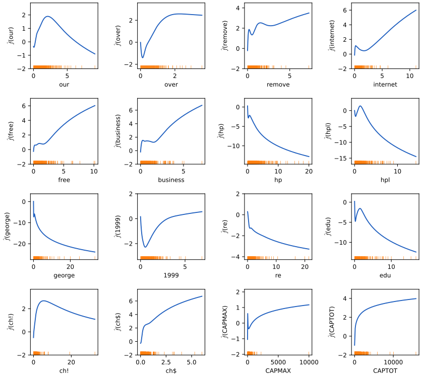
fig_9_1, spam_gam, local_scoring. Reproduces Hastie, Tibshirani and Friedman (2009), Figure 9.1. Download: PDF · SVGTo summarise a term, split \(\hf_j\) into its linear part, the weighted least-squares line of \(\hf_j(x_{ij})\) on \(x_{ij}\) with the final local-scoring weights, and the remaining nonlinear part. Table 9.2 reports the slope, a standard error from the weighted least-squares fit of all the linear parts together, \((\mathbf D^\T\bW\mathbf D)^{-1}\) with \(\mathbf D=(\bone,\bx_1,\dots,\bx_p)\), and \(Z=\) slope/SE; and a test of nonlinearity: the increase of the deviance when term \(j\) alone is made linear (the other smoothing parameters fixed), referred to \(\chi^2\) with \(\df_j-1\approx3\) degrees of freedom.
| Name | Num. | this fit | the book | ||||||
|---|---|---|---|---|---|---|---|---|---|
| df | Coefficient | Std. error | Z | Nonlinear P | Coefficient | Z | Nonlinear P | ||
| Positive effects | |||||||||
| our | 5 | 4.0 | 0.574 | 0.106 | 5.404 | 0.038 | 0.566 | 4.970 | 0.052 |
| over † | 6 | 4.0 | 0.260 | 0.183 | 1.422 | 0.055 | 0.244 | 1.249 | 0.004 |
| remove | 7 | 4.0 | 0.957 | 0.169 | 5.662 | 0.140 | 0.949 | 5.201 | 0.093 |
| internet | 8 | 4.0 | 0.545 | 0.164 | 3.320 | 0.090 | 0.524 | 2.974 | 0.028 |
| free | 16 | 4.0 | 0.500 | 0.118 | 4.229 | 0.038 | 0.507 | 4.010 | 0.065 |
| business | 17 | 4.0 | 0.788 | 0.175 | 4.506 | 0.201 | 0.779 | 4.179 | 0.194 |
| hpl † | 26 | 4.0 | 0.065 | 0.234 | 0.277 | 0.011 | 0.045 | 0.181 | 0.002 |
| 650 | 28 | 4.0 | 0.632 | 0.319 | 1.979 | 0.008 | – | – | – |
| ch! | 52 | 4.0 | 0.667 | 0.119 | 5.619 | 0.197 | 0.674 | 5.283 | 0.164 |
| ch$ | 53 | 4.0 | 1.412 | 0.265 | 5.321 | 0.438 | 1.419 | 5.062 | 0.354 |
| CAPMAX | 56 | 4.0 | 0.270 | 0.213 | 1.270 | 0.005 | 0.247 | 1.080 | 0.000 |
| CAPTOT | 57 | 4.0 | 0.761 | 0.155 | 4.918 | 0.229 | 0.755 | 4.566 | 0.063 |
| Negative effects | |||||||||
| 3d | 4 | 4.0 | -3.860 | 1.656 | -2.330 | 0.001 | – | – | – |
| hp | 25 | 4.0 | -1.435 | 0.211 | -6.814 | 0.259 | -1.404 | -6.262 | 0.140 |
| george | 27 | 4.0 | -5.476 | 0.746 | -7.339 | 0.306 | -5.003 | -6.722 | 0.045 |
| 1999 | 37 | 4.0 | -0.673 | 0.180 | -3.735 | 0.079 | -0.672 | -3.512 | 0.011 |
| project | 44 | 4.0 | -1.063 | 0.390 | -2.726 | 0.765 | – | – | – |
| re | 45 | 4.0 | -0.627 | 0.124 | -5.046 | 0.656 | -0.620 | -4.649 | 0.597 |
| edu | 46 | 4.0 | -1.170 | 0.196 | -5.957 | <0.001 | -1.183 | -5.647 | 0.000 |
| ch; | 49 | 4.0 | -0.065 | 0.376 | -0.173 | 0.001 | – | – | – |
Table 9.2, reproduced: predictors significant at the 0.01 level (two-sided) by the linear or the nonlinear test, together with the book's 16 (†: not significant here). Coefficient: slope of the linear part of \(\hf_j\) on \(\log(x+0.1)\); df: \(\Tr\bS_j-1\) under the final weights. Code: spam_gam_table. Reproduces Hastie, Tibshirani and Friedman (2009), Table 9.2.
The linear parts agree closely with the book: for example our 0.574 (book 0.566), remove 0.957 (0.949), hp −1.435 (−1.404), edu −1.170 (−1.183), ch$ 1.412 (1.419). 18 predictors pass one of the two tests here; 14 of the book's 16 are among them, while over, hpl are not (their nonlinear P-values are above 0.01 here) and 3d, 650, project, ch; are added. The tests are approximate: a likelihood-ratio test for a smoothing-spline term is not exactly \(\chi^2\), and the book's nonlinear P-values come from a different (score-type) approximation, so P-values near 0.01 can fall on either side. Some terms that are not in the table, such as 857 (Z = 0.02 with a standard error of 68), are nearly separating: almost every message with a nonzero value is of one class, the linear coefficient is not identified and the nonlinear test is meaningless.
Filling the gap 9.4: unequal losses, the threshold \(L_{01}/(L_{01}+L_{10})\), and observation weights p. 304
Derivation
Let \(L_{01}\) be the loss for calling a genuine email (class 0) spam and \(L_{10}\) the loss for calling spam email. Given \(x\), predicting 1 has expected loss \(L_{01}\Pr(0\given x)\) and predicting 0 has \(L_{10}\Pr(1\given x)\); the Bayes rule predicts 1 iff \(L_{10}p(x)>L_{01}\{1-p(x)\}\), i.e. iff \(p(x)>L_{01}/(L_{01}+L_{10})\) (Section 2.4 of the book). With \(L_{01}=10\), \(L_{10}=1\) the threshold is \(10/11\). Weights. Fitting with observation weights \(L_{01}\) on class 0 and \(L_{10}\) on class 1 maximises \(\sum_i\omega_i\log\Pr(y_i\given x_i)\); for a flexible enough model its population version is maximised by the conditional probability of the reweighted distribution, \[\tilde p(x)=\frac{L_{10}p(x)}{L_{10}p(x)+L_{01}(1-p(x))},,\] and \(\tilde p(x)>\tfrac12\) is exactly the cost-sensitive Bayes rule above. The difference is that the weighted fit spends its flexibility where the email class needs it. On the test set: the threshold 10/11 on the unweighted fit gives error rates 1.5% in class 0 and 18.3% in class 1 (book 0.8% and 8.7%); the fit with weights 10 on email and threshold \(\tfrac12\) gives 2.0% and 15.8% (book 1.2% and 8.0%). The email error rates are close to the book's, but the spam error rates are about twice as large; whatever the threshold, this fit cannot flag as few as 0.8% of the emails without letting about 32% of the spam through (the ROC curve of Figure 9.6), so the book's pair (0.8%, 8.7%) cannot be obtained from this model on this test set. Note also that the weighted fit trades a little email error for less spam error compared with simply moving the threshold.
After fitting an additive model one should check for interactions, by adding products of the important inputs or automatically with MARS (Section 9.4). By setting \(\df_j=1\) for some terms the analyst moves between linear and partially linear models.
9.1.3 Summary
p. 304 Additive models keep the interpretability of linear models, with the usual inferential tools (Table 9.2), and backfitting lets each input have its own smoother. Their limitation is scale: backfitting fits all \(p\) terms, which is neither feasible nor wise for very many inputs. BRUTO (Hastie and Tibshirani, 1990) adds input selection to backfitting; COSSO (Lin and Zhang, 2006) and SpAM (Ravikumar et al., 2008) use lasso-type penalties to make the additive model sparse (each term is penalised by a norm of the whole function, so whole terms drop out, as in the group lasso); and boosting (Chapter 10, Section 10.3) fits additive models forward stagewise and allows interactions.
9.2 Tree-Based Methods
9.2.1 Background
pp. 305–307 A tree partitions the input space into rectangles and fits a constant in each. Arbitrary partitions into rectangles (top left of Figure 9.2) are hard to describe and to search, so CART (Breiman et al., 1984) restricts itself to recursive binary partitions: split the space in two at \(X_j=s\), then split one or both halves, and so on. The partition is then described by a binary tree, which is easy to read whatever the dimension. With five regions,
\[ \hf(X)=\sum_{m=1}^5c_mI\{(X_1,X_2)\in R_m\}. \tag{9.9} \]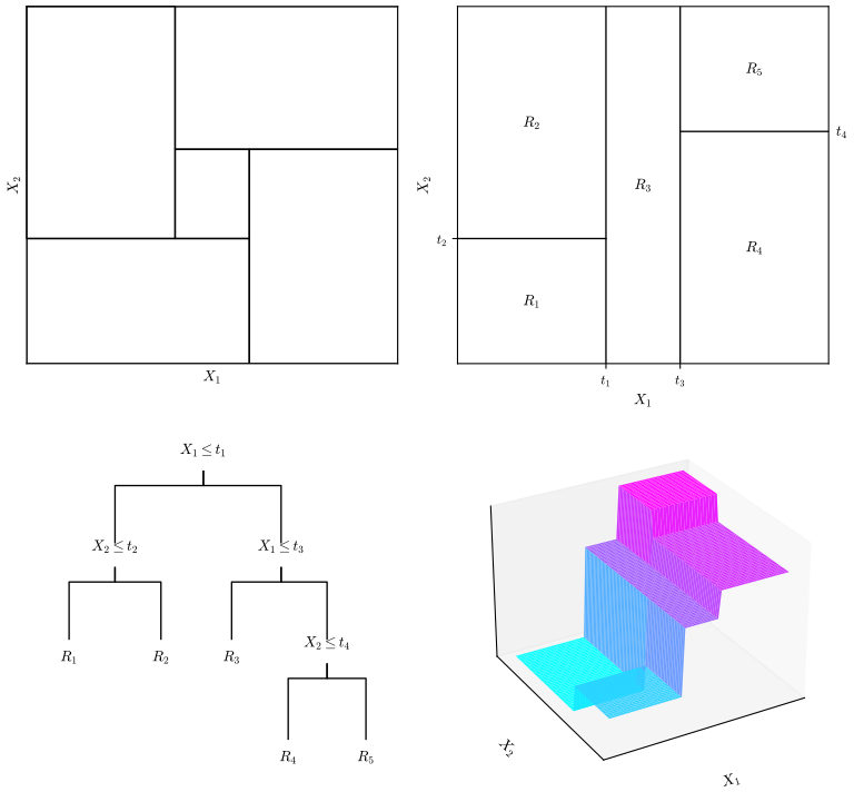
fig_9_2. Reproduces Hastie, Tibshirani and Friedman (2009), Figure 9.2. Download: PDF · SVGSee also (companion course): Bayesian and Probabilistic Machine Learning, Section 14.4, tree-based models, and its trees and committees demonstration.
9.2.2 Regression Trees
pp. 307–308 With a partition into \(M\) regions and a constant in each,
\[ f(x)=\sum_{m=1}^Mc_mI(x\in R_m), \tag{9.10} \]the sum of squares is minimised by the regional means
\[ \hat c_m=\ave(y_i\given x_i\in R_m). \tag{9.11} \]Finding the best partition is computationally infeasible (even for classification with binary inputs, building an optimal tree is NP-complete; Hyafil and Rivest, 1976), so the tree is grown greedily. For a splitting variable \(j\) and split point \(s\) define the half-planes
\[ R_1(j,s)=\{X\given X_j\le s\}\quad\text{and}\quad R_2(j,s)=\{X\given X_j>s\}, \tag{9.12} \]and choose \((j,s)\) to solve
\[ \min_{j,\,s}\Big[\min_{c_1}\sum_{x_i\in R_1(j,s)}(y_i-c_1)^2+\min_{c_2}\sum_{x_i\in R_2(j,s)}(y_i-c_2)^2\Big]. \tag{9.13} \]The inner minimisations are solved by
\[ \hat c_1=\ave(y_i\given x_i\in R_1(j,s))\quad\text{and}\quad\hat c_2=\ave(y_i\given x_i\in R_2(j,s)). \tag{9.14} \]The data are then split in two and the procedure is repeated in each half.
Result 9.4 (the best constants, and one pass finds the best split point) p. 307, (9.11), (9.14)
(a) For any constant \(c\),
\[\sum_{x_i\in R_m}(y_i-c)^2=\sum_{x_i\in R_m}(y_i-\bar y_m)^2+N_m(c-\bar y_m)^2,\]so (9.11) and (9.14) hold. (b) Sort a node's \(n\) values of \(x_j\) once. With the cumulative sums \(S_k=\sum_{l\le k}y_{(l)}\), \(V_k=\sum_{l\le k}y_{(l)}^2\) over the sorted order, the criterion of the split between the \(k\)-th and \((k+1)\)-th values is
\[ \Big(V_k-\frac{S_k^2}{k}\Big)+\Big(V_n-V_k-\frac{(S_n-S_k)^2}{n-k}\Big), \]so every split point of one variable is scored in \(O(n)\) operations after an \(O(n\log n)\) sort; only the \(n-1\) gaps between distinct values matter, and the threshold is reported at the midpoint of the gap.
Proof
(a) Add and subtract \(\bar y_m\): \[\sum(y_i-c)^2=\sum(y_i-\bar y_m)^2+2(\bar y_m-c)\sum(y_i-\bar y_m)+N_m(\bar y_m-c)^2,\] and the middle sum is zero. The minimum over \(c\) is at \(c=\bar y_m\), with value the within-region sum of squares. (b) For the left child (the first \(k\) sorted points) the minimum in (a) is \(\sum y^2-(\sum y)^2/k=V_k-S_k^2/k\), and similarly on the right. Two split points inside the same gap between consecutive distinct values give the same children, so they are equivalent. ∎
See also (companion course): Result 14.8, what one split gains, \(N_LN_R(\bar y_L-\bar y_R)^2/N\).
How big should the tree be? Stopping when no split decreases the sum of squares by much is short-sighted: a useless-looking split can enable a very good one below it (the XOR pattern is the standard example). So grow a large tree \(T_0\), stopping only at a minimum node size, and prune it.
Definition 9.2 (subtrees and cost complexity) p. 308, (9.15)–(9.16)
A subtree \(T\subseteq T_0\) is any tree obtained by collapsing some internal nodes of \(T_0\) (removing everything below them). Its terminal nodes \(m=1,\dots,|T|\) are regions \(R_m\) with
\[ N_m=\#\{x_i\in R_m\},\qquad\hat c_m=\frac1{N_m}\sum_{x_i\in R_m}y_i,\qquad Q_m(T)=\frac1{N_m}\sum_{x_i\in R_m}(y_i-\hat c_m)^2, \tag{9.15} \]and the cost-complexity criterion is
\[ C_\alpha(T)=\sum_{m=1}^{|T|}N_mQ_m(T)+\alpha|T|. \tag{9.16} \]For a node \(t\) of \(T_0\) write \(R(t)\) for its cost as a leaf (\(N_tQ_t\)), \(T_t\) for the branch of the current tree below \(t\), and \(R(T_t)=\sum_{\text{leaves }m\text{ of }T_t}R(m)\). Splitting never increases the cost: \(R(t)\ge R(t_L)+R(t_R)\) (for squared error by Result 9.4(a), because the children's means fit at least as well as the parent's; for misclassification counts because the parent's majority class is one of the candidates in each child).
Result 9.5 (for each \(\alpha\) there is a unique smallest optimal subtree \(T_\alpha\)) p. 308
For \(\alpha\ge0\) define, from the leaves of \(T_0\) upwards, \(V(t)=R(t)+\alpha\) at a leaf of \(T_0\) and \(V(t)=\min\{R(t)+\alpha,\ V(t_L)+V(t_R)\}\) at an internal node. Then \(V(\text{root})=\min_{T\subseteq T_0}C_\alpha(T)\); collapsing exactly the nodes where \(R(t)+\alpha\le V(t_L)+V(t_R)\) (ties resolved by collapsing) gives a minimiser \(T_\alpha\) which is contained in every other minimiser. In particular it is the unique minimiser with the fewest leaves.
Proof
That \(V\) is the optimal cost is dynamic programming: a pruned version of the branch at \(t\) either collapses \(t\) (cost \(R(t)+\alpha\)) or keeps its split, and then consists of independent pruned versions of the two child branches, whose costs add. This is proved in the companion course, Result 14.9. For the minimality, argue by induction from the leaves upwards that the subtree \(T_\alpha(t)\) built by the rule is contained in every optimal pruning of the branch at \(t\). At a leaf this is trivial. At an internal \(t\): if \(R(t)+\alpha\le V(t_L)+V(t_R)\), \(T_\alpha(t)\) is the single node \(t\), which is contained in every pruning. Otherwise \(R(t)+\alpha>V(t_L)+V(t_R)\), so no optimal pruning collapses \(t\); every optimal pruning keeps the split and its two parts must be optimal for the child branches (else replacing a part would lower the cost), so by induction they contain \(T_\alpha(t_L)\) and \(T_\alpha(t_R)\), and hence the pruning contains \(T_\alpha(t)\). A minimiser contained in every minimiser has the fewest leaves, and any other minimiser with that many leaves contains it and so equals it. ∎
Result 9.6 (the optimal subtrees are nested, and weakest-link pruning finds all of them) p. 308
(a) If \(\alpha\le\beta\) then \(T_\beta\subseteq T_\alpha\). (b) Weakest-link pruning: put \(\alpha_0=0\) and \(T^{(0)}=T_0\) with every node of \(g=0\) (below) collapsed; given \(T^{(k)}\), compute for each of its internal nodes
\[ g_k(t)=\frac{R(t)-R(T_t)}{|T_t|-1}, \]the increase in cost per leaf removed by collapsing \(t\); let \(\alpha_{k+1}=\min_tg_k(t)\) and obtain \(T^{(k+1)}\) by collapsing every node attaining the minimum. Then \(0=\alpha_0<\alpha_1<\alpha_2<\dots\) and \(T_\alpha=T^{(k)}\) for every \(\alpha\in[\alpha_k,\alpha_{k+1})\). So the finite sequence \(T^{(0)}\supset T^{(1)}\supset\dots\supset\{\text{root}\}\) contains \(T_\alpha\) for every \(\alpha\ge0\).
Proof
A formula. Let \(T\) be a tree and \(T'\subseteq T\) a pruning of it, obtained by collapsing a set \(\mathcal C\) of internal nodes of \(T\) none of which lies below another. The branches \(T_t\), \(t\in\mathcal C\), are disjoint, and
\[ C_\alpha(T')-C_\alpha(T)=\sum_{t\in\mathcal C}\big\{R(t)+\alpha-R(T_t)-\alpha|T_t|\big\}=\sum_{t\in\mathcal C}(|T_t|-1)\{g(t)-\alpha\}, \]with \(g(t)=\{R(t)-R(T_t)\}/(|T_t|-1)\ge0\) computed in \(T\).
(a) Write \(V_\alpha\) for the function of Result 9.5. For any branch, every pruning has at least one leaf, so increasing \(\alpha\) to \(\beta\) raises the cost of every pruning by at least \(\beta-\alpha\): \(V_\beta(u)\ge V_\alpha(u)+(\beta-\alpha)\) for every node \(u\). Suppose \(T_\alpha\) collapses \(t\), i.e. \(R(t)+\alpha\le V_\alpha(t_L)+V_\alpha(t_R)\). Then \[R(t)+\beta\le V_\alpha(t_L)+V_\alpha(t_R)+(\beta-\alpha)\le V_\beta(t_L)+V_\beta(t_R)-(\beta-\alpha)\le V_\beta(t_L)+V_\beta(t_R),\] so \(T_\beta\) collapses \(t\) too. Every node collapsed in \(T_\alpha\) is collapsed in \(T_\beta\): \(T_\beta\subseteq T_\alpha\).
(b) Induction on \(k\), with the hypothesis that \(T^{(k)}=T_{\alpha_k}\) and that every internal node of \(T^{(k)}\) has \(g_k(t)>\alpha_k\). For \(k=0\) and \(\alpha=0\), the formula with \(\alpha=0\) shows that collapsing nodes with \(g=0\) keeps the cost and collapsing any other node raises it, so the smallest minimiser among the prunings of \(T_0\) is \(T^{(0)}\), and its remaining nodes have \(g>0\) (collapsing a node with \(g=0\) does not change the \(g\) of its ancestors to \(0\); see the last paragraph). Now let \(\alpha\in[\alpha_k,\alpha_{k+1})\). By (a), \(T_\alpha\subseteq T_{\alpha_k}=T^{(k)}\), so \(T_\alpha\) is the smallest minimiser among the prunings of \(T^{(k)}\). By the formula (with \(T=T^{(k)}\)), any proper pruning \(T'\) of \(T^{(k)}\) has \[C_\alpha(T')-C_\alpha(T^{(k)})=\sum_{t\in\mathcal C}(|T_t|-1)\{g_k(t)-\alpha\}>0,\] since every \(g_k(t)\ge\alpha_{k+1}>\alpha\). So \(T_\alpha=T^{(k)}\). At \(\alpha=\alpha_{k+1}\) the same formula is \(\ge0\), with equality exactly when every collapsed node has \(g_k(t)=\alpha_{k+1}\): the minimisers are the prunings that collapse weakest links only, and the smallest collapses all of them, i.e. \(T_{\alpha_{k+1}}=T^{(k+1)}\).
It remains to check that the internal nodes of \(T^{(k+1)}\) have \(g_{k+1}(t)>\alpha_{k+1}\) (this gives \(\alpha_{k+2}>\alpha_{k+1}\) and completes the induction). An internal node \(s\) of \(T^{(k+1)}\) was not a weakest link, so \(R(s)+\alpha_{k+1}>R(T_s)+\alpha_{k+1}|T_s|\) in \(T^{(k)}\). Collapsing weakest links below \(s\) does not change \(R(T_s)+\alpha_{k+1}|T_s|\) (each collapse changes it by \((|T_t|-1)(g_k(t)-\alpha_{k+1})=0\)), so in \(T^{(k+1)}\) still \(R(s)+\alpha_{k+1}>R(T'_s)+\alpha_{k+1}|T'_s|\), i.e. \(g_{k+1}(s)>\alpha_{k+1}\). The sequence is finite because each step removes at least one node. ∎
This is the result the book attributes to Breiman et al. (1984) and Ripley (1996). It is why pruning is cheap: one pass of weakest-link pruning yields the whole path \(\alpha\mapsto T_\alpha\), a step function with a few dozen distinct trees. The code (Tree.prune_sequence) implements it, and checking it against an exhaustive search over all the prunings of a small tree, for hundreds of values of \(\alpha\), confirms that the sequence contains every \(T_\alpha\).
Filling the gap 9.5: cross-validation indexed by \(\alpha\) p. 308, p. 313
How the cross-validation of Figure 9.4 is organised
The tree size is not a good index for cross-validation: the tree grown on nine tenths of the data has its own pruning sequence, whose sizes need not match those of \(T_0\). The penalty \(\alpha\) means the same thing in every fold, so: (1) compute the breakpoints \(\alpha_k\) of the full-data tree; (2) for each fold \(v\), grow \(T_0^{(-v)}\) on the other folds, take its optimal subtree at \(\tilde\alpha_k=\sqrt{\alpha_k\alpha_{k+1}}\) (a value inside the interval where the full-data tree is \(T^{(k)}\), as Breiman et al. (1984) recommend) and count its errors on fold \(v\); (3) sum over folds to get the cross-validated error of \(T^{(k)}\), and plot it against \(|T^{(k)}|\). The standard error is the standard deviation of the ten fold error rates divided by \(\sqrt{10}\). The one-standard-error rule picks the smallest tree whose cross-validated error is within one standard error of the minimum.
9.2.3 Classification Trees
pp. 308–310 For a response with classes \(1,\dots,K\) only the splitting and pruning criteria change. In node \(m\), with region \(R_m\) and \(N_m\) observations, let
\[ \hat p_{mk}=\frac1{N_m}\sum_{x_i\in R_m}I(y_i=k), \]the proportion of class \(k\), and classify the node to the majority class \(k(m)=\argmax_k\hat p_{mk}\).
Definition 9.3 (node impurity measures) p. 309, (9.17)
\[ \begin{aligned}&\text{Misclassification error:}&&\frac1{N_m}\sum_{i\in R_m}I(y_i\ne k(m))=1-\hat p_{mk(m)},\\&\text{Gini index:}&&\sum_{k\ne k'}\hat p_{mk}\hat p_{mk'}=\sum_{k=1}^K\hat p_{mk}(1-\hat p_{mk}),\\&\text{Cross-entropy or deviance:}&&-\sum_{k=1}^K\hat p_{mk}\log\hat p_{mk}.\end{aligned} \tag{9.17} \]For two classes with \(p\) the proportion of the second class these are \(1-\max(p,1-p)\), \(2p(1-p)\) and \(-p\log p-(1-p)\log(1-p)\). A split of node \(m\) is scored by \(N_{mL}Q_{mL}+N_{mR}Q_{mR}\), the impurities of the children weighted by their sizes, as in (9.13).
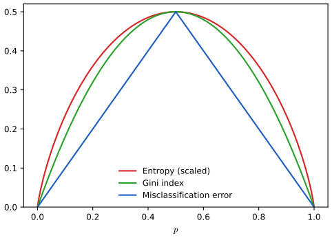
fig_9_3. Reproduces Hastie, Tibshirani and Friedman (2009), Figure 9.3. Download: PDF · SVGResult 9.7 (why Gini and deviance prefer purer splits) pp. 309–310
Let \(i(\mathbf p)\) be the Gini index or the entropy, functions of the class-proportion vector. Both are strictly concave, so for any split \(N\,i(\mathbf p)\ge N_L\,i(\mathbf p_L)+N_R\,i(\mathbf p_R)\), with equality only when \(\mathbf p_L=\mathbf p_R\): every split that changes the class proportions lowers the impurity. The misclassification rate is concave but piecewise linear: a split whose children have the same majority class as the parent does not change it at all. In the book's example, a node with \((400,400)\) split into \((300,100),(100,300)\) or into \((200,400),(200,0)\): both splits have misclassification rate \(0.25\), but the Gini indices are \(0.375\) and \(\tfrac13\) and the entropies \(0.562\) and \(0.477\) nats; both measures prefer the second split, which creates a pure node.
Proof sketch (full proof in the companion course)
The parent's proportions are the mixture \(\mathbf p=a\mathbf p_L+(1-a)\mathbf p_R\), \(a=N_L/N\); by strict concavity (Jensen's inequality) \(i(\mathbf p)\ge a\,i(\mathbf p_L)+(1-a)\,i(\mathbf p_R)\), strictly unless \(\mathbf p_L=\mathbf p_R\). The misclassification rate \(\min_k(1-p_k)\) is linear on the region where a given class is the majority. Proved in full as Result 14.10 of the companion course. Numbers. First split: each child has \(p=\tfrac14\), Gini \(2\cdot\tfrac14\cdot\tfrac34=0.375\), entropy \(-\tfrac14\log\tfrac14-\tfrac34\log\tfrac34=0.5623\). Second split: the child \((200,400)\) has \(p=\tfrac13\), Gini \(\tfrac49\) and entropy \(0.6365\), the pure child has 0; weighting by \(\tfrac{600}{800}\) gives \(\tfrac13\) and \(0.4774\). ∎
So Gini or deviance is used to grow the tree; any of the three can guide cost-complexity pruning, and the misclassification rate is the usual choice because it is what one cares about in the end. The book's other reason for preferring Gini and entropy, differentiability, matters for numerical optimisation over soft or oblique splits rather than for the exhaustive search over split points.
Filling the gap 9.6: two interpretations of the Gini index p. 310
Derivation
A randomised rule. Classify each observation of the node to class \(k\) with probability \(\hat p_{mk}\), independently of its label. An observation of class \(k\) (a fraction \(\hat p_{mk}\) of the node) is misclassified with probability \(1-\hat p_{mk}=\sum_{k'\ne k}\hat p_{mk'}\), so the expected training error rate is \[\sum_k\hat p_{mk}\sum_{k'\ne k}\hat p_{mk'}=\sum_{k\ne k'}\hat p_{mk}\hat p_{mk'},\] the Gini index. Variances. Code each observation as \(Z_k=I(y=k)\). Over the node, \(Z_k\) has mean \(\hat p_{mk}\) and (population) variance \(\hat p_{mk}(1-\hat p_{mk})\), and the sum over \(k\) is the Gini index: growing a classification tree with the Gini index is growing a regression tree for the \(K\) indicator responses with squared error. The two forms agree because \[\sum_{k\ne k'}p_kp_{k'}=(\sum_kp_k)^2-\sum_kp_k^2=1-\sum_kp_k^2=\sum_kp_k(1-p_k).\] ∎
9.2.4 Other Issues
pp. 310–313 Categorical predictors. A predictor with \(q\) unordered levels can be split into two groups in \(2^{q-1}-1\) ways. For two classes, and for squared error, there is a shortcut.
Result 9.8 (the ordering trick for categorical predictors) p. 310
Let a node contain \(n_\ell\gt0\) observations at level \(\ell=1,\dots,q\) of a categorical input. (a) Two classes: let \(m_\ell\) be the number of class-1 observations at level \(\ell\) and order the levels by \(\hat p_\ell=m_\ell/n_\ell\). For any impurity \(i(p)\) that is concave in the class-1 proportion \(p\) (Gini, entropy, misclassification), among all \(2^{q-1}-1\) splits a best one puts the levels with the \(k\) smallest \(\hat p_\ell\) on one side, for some \(k\). (b) Squared error: the same holds with the levels ordered by their mean response (Fisher, 1958). (c) With three or more classes no such ordering exists in general.
Proof
Write \(\psi(n,m)=n\,i(m/n)\) for \(n>0\) (and \(\psi(0,0)=0\)); \(\psi\) is the perspective of the concave function \(i\), hence concave on \(\{(n,m):0\le m\le n\}\), and it is positively homogeneous. A split sends a set \(L\) of levels left; with \(u_\ell=(n_\ell,m_\ell)\) and \(v_L=\sum_{\ell\in L}u_\ell\), its total impurity is
\[ J(L)=\psi(v_L)+\psi(U-v_L),\qquad U=\sum_\ell u_\ell, \]a concave function \(F(v)=\psi(v)+\psi(U-v)\) evaluated at the point \(v_L\). The \(2^q\) points \(v_L\) all lie in the zonotope \(Z=\{\sum_\ell\lambda_\ell u_\ell:0\le\lambda_\ell\le1\}\), a convex polygon, and each vertex of \(Z\) is one of them: a vertex is the unique maximiser over \(Z\) of some linear functional \(c^\T v\), and \(c^\T\sum_\ell\lambda_\ell u_\ell\) is maximised by \(\lambda_\ell=1\) when \(c^\T u_\ell\gt0\) and \(\lambda_\ell=0\) when \(c^\T u_\ell\lt0\) (uniqueness rules out \(c^\T u_\ell=0\)), so the vertex is \(v_L\) with \(L=\{\ell:c^\T u_\ell\gt0\}\). A concave function attains its minimum over a polygon at a vertex (any point is a convex combination of vertices, and \(F\) at that point is at least the smallest value at the vertices). Since every \(v_L\) lies in \(Z\), the minimum of \(J\) over all \(L\) equals the minimum of \(F\) over the vertices, and is attained at some vertex set \(L=\{\ell:c_1n_\ell+c_2m_\ell\gt0\}\). Dividing by \(n_\ell\gt0\), this is \(\{\ell:c_1+c_2\hat p_\ell\gt0\}\): if \(c_2\gt0\), the levels with \(\hat p_\ell\) above a threshold; if \(c_2\lt0\), those below; if \(c_2=0\), all or none. Every such set is a lower or an upper segment of the ordering by \(\hat p_\ell\), which proves (a). The trivial sets (all or none) give the parent's impurity, which is never below that of a real split (\(\psi\) is superadditive: concave and homogeneous), so a nontrivial ordered split is optimal. (b) For squared error, \(J(L)=\sum y^2-S_L^2/N_L-S_R^2/N_R\) with \(u_\ell=(n_\ell,s_\ell)\), \(s_\ell\) the sum of the responses at level \(\ell\); \(\psi(n,s)=-s^2/n\) is concave (it is the perspective of \(-s^2\)), and the same argument orders the levels by \(s_\ell/n_\ell\). (c) With \(K\) classes, \(u_\ell\in\R^K\) and the vertices of a zonotope in more than two dimensions are not cut out by a single ordering of the levels. ∎
The computation drops from \(2^{q-1}-1\) splits to \(q-1\). An exhaustive check on hundreds of random tables in the code confirms (a) and (b) for Gini, entropy and squared error, and finds three-class tables where ordering the levels by one class proportion misses the best split. The many possible splits of a predictor with many levels are also a danger: the more partitions, the likelier one of them fits the noise well, so such predictors are favoured and overfit.
Filling the gap 9.7: the loss matrix pp. 310–311
Why the loss-weighted Gini index does nothing for two classes, what weights do, and the Bayes rule in a node
The loss-weighted Gini index \(\sum_{k\ne k'}L_{kk'}\hat p_{mk}\hat p_{mk'}\) is the expected loss of the randomised rule of Filling the gap 9.6. With two classes it is \((L_{01}+L_{10})\hat p_{m0}\hat p_{m1}\), a constant multiple of the Gini index, so it chooses the same splits. Weights. Weighting class-\(k\) observations by \(L_{k,1-k}\) replaces the counts by weighted counts: in every node the class-\(k\) proportion becomes \(L_{k,1-k}N_{mk}/\sum_lL_{l,1-l}N_{ml}\), exactly the proportion that a population with prior \(\pi_k\propto L_{k,1-k}\pi_k\) would show. So weights act as altered priors, and they change the splits as well as the leaf labels. With more classes this works only if \(L_{kk'}\) does not depend on \(k'\). Bayes rule in a leaf. Predicting class \(k\) for the observations of node \(m\) costs on average \(\sum_\ell L_{\ell k}\hat p_{m\ell}\), so the leaf is labelled \(k(m)=\argmin_k\sum_\ell L_{\ell k}\hat p_{m\ell}\); with two classes, class 1 iff \(\hat p_{m1}\ge L_{01}/(L_{01}+L_{10})\) (Filling the gap 9.4).
Missing predictor values. Instead of discarding incomplete observations or imputing, trees offer two remedies: a separate category "missing" for a categorical input (which also reveals whether missingness is informative), and surrogate splits.
Filling the gap 9.8: surrogate splits, computed p. 311
Definition, and the surrogates of the spam tree's first split
For a node with primary split \(x_j\lt s\), and another input \(x_{j'}\), consider the splits \(x_{j'}\lt s'\) and \(x_{j'}\ge s'\) and measure each by its agreement: the fraction of the node's training observations (with both inputs present) that it sends the same way as the primary split. The best surrogate on \(x_{j'}\) maximises the agreement; surrogates are ranked by it, and only those beating the "go with the majority" rule are useful. An observation missing \(x_j\) is sent down by the first surrogate whose input it has. On the spam tree's root split \(\texttt{ch\$}<0.0555\), 74.9% of the training messages go left, so that is the baseline; the best surrogates are \(\texttt{000}<0.055\) (agreement 83.7%), \(\texttt{money}<0.035\) (83.0%) and \(\texttt{receive}<0.04\) (79.0%): all three words, like "$", mark commercial mail, which is the correlation that surrogates exploit (surrogate_splits).
Why binary splits? Multiway splits fragment the data too fast, and any multiway split can be built from binary ones. Other procedures. C4.5 and C5.0 (Quinlan, 1993) grow similar trees and can turn a tree into a set of simplified rules. Linear combination splits \(\sum_ja_jX_j\le s\) can predict better but are harder to read and to optimise; Section 9.5 offers a smooth alternative.
Filling the gap 9.9: the instability of trees, measured p. 312
Why a hierarchy of greedy choices has high variance, and 100 bootstrap trees for the spam data
Each split is the argmin of a criterion over many candidates whose values are close; a small perturbation of the data can change the winner, and every split below it is then computed on a different subset of the data, so the change propagates down the tree. A smooth model has no such discontinuity: a small change in the data changes the fit a little. We grew the spam tree (same settings as Figure 9.4) on 100 bootstrap samples of the training data. The root split was \(\texttt{ch\$}<0.0555\) in 45 of them and another threshold on ch$ (from 0.045 to 0.0595) in 34 more, but in 21 the root was ch!; the pair of variables used at the second level was (remove, hp) in only 53 trees, with (ch!, hp) in 26 and (remove, ch$) in 14. The 17-leaf pruned bootstrap trees had test errors from 8.5% to 11.5% (mean 9.8%). Averaging many such trees (bagging, Section 8.7, with its bagging demonstration) reduces this variance. In the companion course, Foundations of Deep Learning, Section 9.6 treats model averaging in general.
Lack of smoothness. The fitted surface is piecewise constant, which matters little for classification but costs accuracy in regression, where the true function is usually smooth; MARS is a remedy.
Filling the gap 9.10: why trees find additive structure hard p. 313
Counting the splits an additive function needs
Let \(Y=c_1I(X_1\lt t_1)+c_2I(X_2\lt t_2)+\varepsilon\). The regression function takes four values on the four quadrants around \((t_1,t_2)\), so a tree needs at least four leaves: a split at \(t_1\), then a split at \(t_2\) in both children, three splits for two additive effects. With \(k\) such effects \(\sum_{j}c_jI(X_j\lt t_j)\) the function takes \(2^k\) values (generically all different), so a tree needs \(2^k\) leaves and \(2^k-1\) splits, the same split repeated in \(2^{j-1}\) branches at depth \(j\), each estimated from a fraction \(2^{-(j-1)}\) of the data; ten effects need 1023 splits where a sum of ten step functions has ten. Nothing in greedy growing encourages the repetition, and the resulting tree hides the additive structure. MARS (Section 9.4) drops the tree constraint to capture it.
9.2.5 Spam Example (Continued)
pp. 313–317 A classification tree was grown on the 3065 training messages with the deviance (a node is split if it has at least 10 observations and a deviance of at least 1% of the root's, and children need at least 5 observations) and pruned with the misclassification rate. The grown tree has 63 leaves; collapsing the splits that do not change the misclassification count leaves 44 (\(\alpha=0\)). The weakest-link sequence then has breakpoints \(\alpha\) = 2, 2.25, 2.33, 3, 3.6, 4, 5, 5.43, 7, 10, 14, 21, 34, 51, 176 and 601, with 41, 33, 30, 26, 21, 18, 17, 10, 9, 8, 7, 6, 5, 3, 2 and 1 leaves; the book's top axis in Figure 9.4 marks 176, 21, 7, 5, 3, 2 and 0, all of which are breakpoints here.
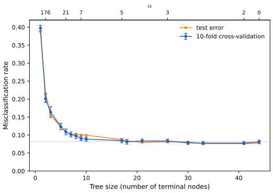
numpy.random.default_rng(2); other fold assignments give 18 or 26 leaves, a reminder of how flat the curve is. Code: fig_9_4, spam_tree, cv_tree. Reproduces Hastie, Tibshirani and Friedman (2009), Figure 9.4. Download: PDF · SVGThe book settles on the 17-leaf tree, the next smaller member of the sequence, shown in Figure 9.5. Its splits are almost those of the book's tree: the first six (ch$, remove, hp, ch!, george, CAPAVE) and the test-set sizes of every node they define agree exactly; lower down, the two trees prune different branches (ours keeps splits on pm and money where the book keeps CAPAVE and 1999 under the right branch), the instability of Filling the gap 9.9 at work.
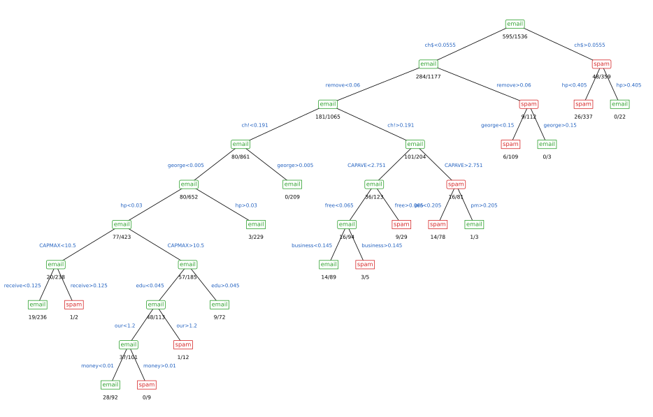
fig_9_5, _draw_tree. Reproduces Hastie, Tibshirani and Friedman (2009), Figure 9.5. Download: PDF · SVGNote on Figure 9.5: the root count does not add up p. 315
In a tree, the misclassified test messages of an email node are the spam messages in it, so the root's count must equal the spam in its two children. The book's figure shows 280/1177 for the email child (280 spam) and 48/359 for the spam child (\(359-48=311\) spam), so the root should show \(280+311=591\), not 600; similarly its node remove<0.06 (280/1177) has children 180/1065 and 9/112, which contain \(180+103=283\) spam, not 280. With the test set of the book's website the counts are consistent: 595 = 284 + 311 at the root, and every node size in the book's figure (1177, 359, 1065, 861, 652, ...) is reproduced exactly.
| Test data (1536) | predicted email | predicted spam |
|---|---|---|
| true email | 57.4% | 3.9% |
| true spam | 4.8% | 33.9% |
Table 9.3, reproduced: confusion rates of the 17-leaf tree on the test data. Overall error 8.7% (134 of 1536; book 9.3%), about 60% higher than the additive model's 5.5%. Reproduces Hastie, Tibshirani and Friedman (2009), Table 9.3.
Treating spam as the "disease", the sensitivity and the specificity are
\[\Pr(\text{predict spam}\given\text{spam})=\frac{33.9}{33.9+4.8}=87.6\%,\qquad\Pr(\text{predict email}\given\text{email})=\frac{57.4}{57.4+3.9}=93.6\%\](book 86.3% and 93.4%). Varying the loss \(L_{01}\) from 0.1 to 10 with \(L_{10}=1\) changes the leaf threshold \(L_{01}/(L_{01}+L_{10})\) and traces the ROC curve, sensitivity against specificity; for a tree it has one point per distinct leaf proportion.
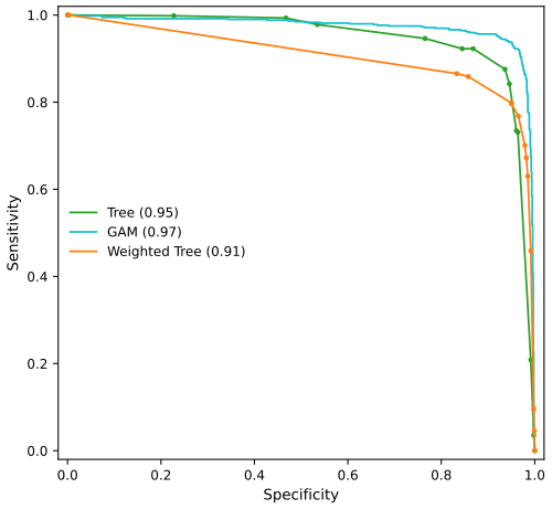
fig_9_6, roc_points, spam_weighted_tree. Reproduces Hastie, Tibshirani and Friedman (2009), Figure 9.6. Download: PDF · SVGThe standard error of a sensitivity or specificity near 0.9 estimated from about 1536 test cases is about \(\sqrt{0.9\cdot0.1/1536}=0.008\), so differences between curves of about 0.02 are meaningful. The GAM dominates both trees. The weighted tree is better than the unweighted one at very high specificity, the region that matters when losing a genuine email is costly, and worse elsewhere. Classified by its own Bayes rule it misclassifies 2.1% of the emails and 29.9% of the spam.
Result 9.9 (the area under the ROC curve is a Mann–Whitney statistic) p. 317
Let a rule assign scores \(s\) and predict class 1 when \(s\ge c\); let \(s_1,\dots,s_{n_1}\) be the scores of the class-1 cases and \(r_1,\dots,r_{n_0}\) those of the class-0 cases. The area under the ROC curve, drawn through the points \((\text{specificity}(c),\text{sensitivity}(c))\) for all thresholds and joined by straight lines, is
\[ \text{AUC}=\frac1{n_1n_0}\sum_{a=1}^{n_1}\sum_{b=1}^{n_0}\Big\{I(s_a>r_b)+\tfrac12I(s_a=r_b)\Big\}, \]an estimate of \(\Pr(S_1>S_0)+\tfrac12\Pr(S_1=S_0)\) for independent scores of a random case and a random non-case, and \(n_1n_0\,\text{AUC}\) is the Mann–Whitney \(U\) statistic (equivalently the Wilcoxon rank-sum statistic minus \(n_1(n_1+1)/2\)).
Proof
Plot the curve as sensitivity against \(1-\)specificity (the false-positive rate); reflecting the axis does not change the area. Lower the threshold through the distinct score values \(v_1\gt v_2\gt\dots\). At \(v_k\) the true-positive rate rises by \(a_k/n_1\) and the false-positive rate by \(b_k/n_0\), where \(a_k\) and \(b_k\) count the class-1 and class-0 scores equal to \(v_k\). The trapezoid over this step has area \(\frac{b_k}{n_0}\cdot\frac1{n_1}\big(A_{k-1}+\tfrac12a_k\big)\), where \(A_{k-1}=\sum_{l\lt k}a_l\) is the number of class-1 scores above \(v_k\). Summing over \(k\): each class-0 score \(r_b=v_k\) contributes \(\frac1{n_1n_0}\{\#\{a:s_a>r_b\}+\tfrac12\#\{a:s_a=r_b\}\}\), which is the double sum. For the rank form, rank all \(n_1+n_0\) scores with mid-ranks for ties; the rank of \(s_a\) is \(1+\#\{s_{a'}\lt s_a\}+\#\{r_b\lt s_a\}+\tfrac12(\text{ties})\), and summing over \(a\) gives \(n_1(n_1+1)/2+U\). ∎
Both computations give 0.9728 for the GAM and 0.9475 for the tree in the code. The book's further remark, that a predictor can change the deviance a lot and the area little, is borne out by its george example: AUC summarises the ranking of cases, and a term that matters for a minority of cases moves it only slightly.
9.3 PRIM: Bump Hunting
pp. 317–320 A regression tree makes the box means as different as possible. The patient rule induction method (PRIM; Friedman and Fisher, 1999) looks instead for boxes where the response mean is high: bump hunting (for minima, use \(-y\)). Its boxes are not organised in a tree, which makes the collection harder to read but each rule simpler.
Algorithm 9.3 (patient rule induction method) p. 320
- Start with all the training data and a maximal box containing all of it.
- Consider shrinking the box by compressing one face, so as to peel off the proportion \(\alpha\) of observations with either the highest or the lowest values of a predictor \(X_j\). Choose the peeling that produces the highest response mean in the remaining box (typically \(\alpha=0.05\) or \(0.10\)).
- Repeat step 2 until some minimal number of observations (say 10) remain in the box.
- Expand the box along any face, as long as the resulting box mean increases (pasting).
- Steps 1–4 give a sequence of boxes with different numbers of observations. Use cross-validation to choose a member of the sequence. Call the box \(B_1\).
- Remove the data in \(B_1\) and repeat steps 2–5 to obtain a second box, and so on.
In the code a peel on face \(j\) moves the face to the \((k+1)\)-th smallest (or largest) value of \(x_j\) in the box, \(k=\max(1,\lfloor\alpha n\rfloor)\), so it removes \(k\) observations, or fewer if values are tied at the new face; a face that would remove nothing is not a candidate. A two-class response is coded 0/1.
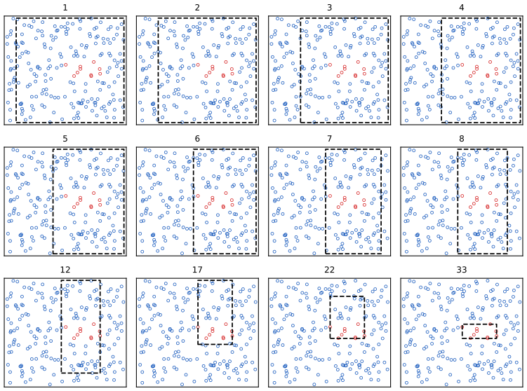
numpy.random.default_rng(7); the book's run stops after 27 peels. Code: fig_9_7, prim_peel. Reproduces Hastie, Tibshirani and Friedman (2009), Figure 9.7. Download: PDF · SVG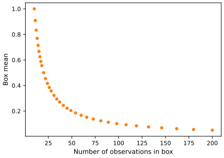
fig_9_8. Reproduces Hastie, Tibshirani and Friedman (2009), Figure 9.8. Download: PDF · SVGPRIM handles categorical inputs by considering all two-group partitions of their levels, as CART does, and missing values in the same way. For \(K\gt2\) classes one runs PRIM separately for each class against a baseline.
Filling the gap 9.11: PRIM's patience, counted p. 320
Derivation of \(\log_2N-1\), \(-\log N/\log(1-\alpha)\) and the 29 peels
Trees. If every split halves the data, after \(d\) levels each node has \(N/2^d\) observations; a node needs at least 2 to be split, so the depth reachable along any path is \(d=\log_2N-1\): 6 for \(N=128\). PRIM. Each peel keeps a fraction \(1-\alpha\), so after \(m\) peels about \(N(1-\alpha)^m\) remain; this reaches one observation when \(m=-\log N/\log(1-\alpha)\), which is \[\log128/(-\log0.9)=4.852/0.1054=46.05\] for \(N=128\), \(\alpha=0.1\). Integer counts. A box of \(n\) points loses \(\max(1,\lfloor0.1n\rfloor)\): \[128\to116\to105\to95\to86\to78\to71\to64\to58\to53\to48\to44\to40\to36\to33\to30\to27\to25\to23\to21\to19\to18\to\dots\to10:\] 20 peels to reach 19 and then one observation at a time, 29 peels down to 10 observations (the minimum box of Algorithm 9.3), the book's number. Either way PRIM spends many small steps where a tree spends a few large ones, so a mistaken early decision costs less.
9.3.1 Spam Example (Continued)
pp. 320–321 PRIM with \(\alpha=0.1\) on the spam training data (response 1 for spam). To choose a box from the peeling sequence we cross-validated the box mean (10 folds: peel on nine, average the response of the held-out tenth inside the box of matching support) and took the largest box whose cross-validated mean is at least 0.95, then pasted it; box 2 repeats this on the training messages outside box 1.
| mean outside the earlier boxes (training; test) | box mean (training; test) | box support (training; test) | |
|---|---|---|---|
| Rule 1 | 0.3974; 0.3874 | 0.9674; 0.9452 | 0.2300; 0.2376 |
| Rule 2 | 0.2271; 0.2135 | 0.9857; 0.8454 | 0.0685; 0.0632 |
PRIM on the spam data. Support: fraction of all training (test) messages in the box. Code: spam_prim, prim_peel, prim_paste. Reproduces the PRIM rule tables of Hastie, Tibshirani and Friedman (2009), Section 9.3.1.
Rule 1 (in order of importance, measured by the drop of the training box mean when the bound is removed): edu ≤ 0.28, CAPTOT ≥ 74, CAPAVE ≥ 2.211, hp ≤ 0, george ≤ 0, you ≥ 0.4, 1999 ≤ 0.1, hpl ≤ 0.23, CAPMAX ≥ 9. Rule 2 has 18 bounds; the most important are hp ≤ 0.11, edu ≤ 0.09, CAPTOT ≥ 54, 1999 ≤ 0.2, george ≤ 0.2. Together the two boxes hold 30.1% of the test messages, 92.4% of them spam.
Box 1 is less pure than the book's (which was 100% spam on its test data, with support 15%) but more than half as large again; its rules involve the same kind of inputs as the book's (capital-letter runs, edu, 1999, you/your, and the absence of hp, george and hpl). The book's own split of the data differs from the website's (its training and test means, 0.3931 and 0.3958, correspond to 1205 and 608 spam rather than 1218 and 595). Box 2, built from the remaining data, is chosen by the same rule but is much less reliable: 98.6% spam in training but 84.5% on the test data, a reminder that a box with a dozen rules fitted to what is left over is easily overfitted. As in the book, the top splitting variables of the tree (ch$, remove) do not appear in PRIM's first box.
9.4 MARS: Multivariate Adaptive Regression Splines
pp. 321–326 MARS (Friedman, 1991) is a forward stepwise linear regression in an adaptively built basis of piecewise linear functions, and also a modification of CART that is better at regression.
Definition 9.4 (reflected pairs and the MARS model) pp. 321–322, (9.18)–(9.19)
For a knot \(t\) the reflected pair is \((x-t)_+\) and \((t-x)_+\), where \((x-t)_+=x-t\) if \(x\gt t\) and 0 otherwise. The candidate set is the collection of reflected pairs in each input with knots at the observed values,
\[ \mathcal C=\{(X_j-t)_+,(t-X_j)_+\}_{t\in\{x_{1j},x_{2j},\dots,x_{Nj}\},\ j=1,2,\dots,p}, \tag{9.18} \]with \(2Np\) functions when all input values are distinct. A MARS model is
\[ f(X)=\beta_0+\sum_{m=1}^M\beta_mh_m(X), \tag{9.19} \]where each \(h_m\) is a function in \(\mathcal C\) or a product of such functions, each input appearing at most once in a product.
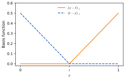
fig_9_9. Reproduces Hastie, Tibshirani and Friedman (2009), Figure 9.9. Download: PDF · SVGThe forward pass. Start with \(\mathcal M=\{h_0=1\}\). At each stage consider every product of a term \(h_\ell\in\mathcal M\) with a reflected pair in \(\mathcal C\) (on an input not already in \(h_\ell\)), and add to the model the pair
\[ \hat\beta_{M+1}h_\ell(X)\cdot(X_j-t)_++\hat\beta_{M+2}h_\ell(X)\cdot(t-X_j)_+,\qquad h_\ell\in\mathcal M, \]that gives the largest decrease in the residual sum of squares, all coefficients being refitted by least squares. Continue until \(\mathcal M\) has a preset number of terms. At the first stage the parent can only be the constant; if the winner is \((X_2-x_{72})_+\) and \((x_{72}-X_2)_+\), the next stage can also multiply these two by new pairs, producing for example \((X_1-x_{51})_+\cdot(x_{72}-X_2)_+\) (Figure 9.11). Figure 9.10 of the book is a diagram of this search and is not redrawn.
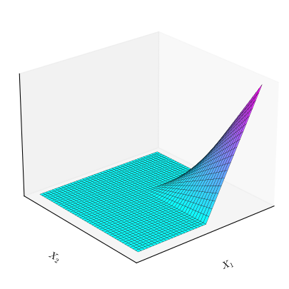
fig_9_11. Reproduces Hastie, Tibshirani and Friedman (2009), Figure 9.11. Download: PDF · SVGResult 9.10 (every knot of an input is scored in one pass) p. 325
Let the current model have \(r\) terms with an orthonormal basis \(\bQ\) (\(N\times r\)) of their span and residual \(\br=\by-\bQ\bQ^\T\by\). For a parent \(h\) and an input \(x\), and a knot \(t\), put \(\bb_+=h\cdot(x-t)_+\), \(\bb_-=h\cdot(t-x)_+\) (as vectors over the data), \(\mathbf c_\pm=\bQ^\T\bb_\pm\), \(g_\pm=\br^\T\bb_\pm\) and \(n_\pm=\|\bb_\pm\|^2\). Adding the pair decreases the RSS by
\[ \Delta(t)=\mathbf g^\T\mathbf G^{-1}\mathbf g,\qquad\mathbf g=\begin{pmatrix}g_+\\g_-\end{pmatrix},\quad\mathbf G=\begin{pmatrix}n_+-\|\mathbf c_+\|^2&-\mathbf c_+^\T\mathbf c_-\\-\mathbf c_+^\T\mathbf c_-&n_--\|\mathbf c_-\|^2\end{pmatrix}. \]With the observations sorted by \(x\), every quantity is a difference of cumulative sums: for example \[\mathbf c_+(t)=\sum_{x_i\gt t}h_i\bQ_{i\cdot}^\T x_i-t\sum_{x_i\gt t}h_i\bQ_{i\cdot}^\T\] and \[n_+(t)=\sum_{x_i\gt t}h_i^2x_i^2-2t\sum_{x_i\gt t}h_i^2x_i+t^2\sum_{x_i\gt t}h_i^2.\] So all knots of one (parent, input) pair cost \(O(Nr)\) operations, instead of \(O(N^2r)\) for refitting at every knot.
Proof
Adding columns \(\bb_+,\bb_-\) to a least-squares fit with orthonormal \(\bQ\): the new fit is the old one plus the projection of \(\br\) on the part of \(\text{span}(\bb_+,\bb_-)\) orthogonal to \(\bQ\), spanned by \(\tilde{\bb}_\pm=\bb_\pm-\bQ\mathbf c_\pm\). The RSS drops by \[\|\text{proj}\|^2=\tilde{\mathbf g}^\T(\tilde{\bB}^\T\tilde{\bB})^{-1}\tilde{\mathbf g}\] with \(\tilde{\bB}=(\tilde{\bb}_+,\tilde{\bb}_-)\), \(\tilde{\mathbf g}=\tilde{\bB}^\T\br\). Because \(\br\perp\bQ\), \(\tilde{\bb}_\pm^\T\br=\bb_\pm^\T\br=g_\pm\). The Gram entries are \(\|\tilde{\bb}_\pm\|^2=n_\pm-\|\mathbf c_\pm\|^2\) and \[\tilde{\bb}_+^\T\tilde{\bb}_-=\bb_+^\T\bb_--\mathbf c_+^\T\mathbf c_-=-\mathbf c_+^\T\mathbf c_-,\] since \(\bb_+\) and \(\bb_-\) have disjoint supports (\(x\gt t\) and \(x\lt t\)): this is \(\mathbf G\). (If one member is zero or in the span of \(\bQ\), use the other alone, \(\Delta=g^2/(n-\|\mathbf c\|^2)\).) Each entry is linear in a few sums over \(\{x_i\gt t\}\) or \(\{x_i\lt t\}\) whose coefficients are polynomials in \(t\), e.g. \(h_i(x_i-t)=h_ix_i-th_i\); prefix sums over the sorted order give all of them for every \(t\) in one pass of \(O(Nr)\) operations (the \(\bQ\)-weighted sums are \(r\)-vectors), after which each knot costs \(O(r)\). This is the "update in \(O(1)\) as the knot moves" of the book, for \(r\) fixed. ∎
The code keeps knots at every observed value, apart from Friedman's (1991) safeguards: no knots among the \(L_e=3-\log_2(0.05/p)\) extreme values of each input (endspan) and, within a parent's support of \(N_m\) points, knots at most every \(L=-\log_2[-\log(0.95)/(pN_m)]/2.5\) observations (minspan), which limit the variance of knots placed in sparse regions. A brute-force refit at every knot gives the same winner and the same drop in RSS.
The backward pass. The final forward model usually overfits. The term whose removal increases the RSS least is deleted, one at a time, giving the best model \(\hf_\lambda\) of each size \(\lambda\); the size is chosen by generalised cross-validation,
\[ \GCV(\lambda)=\frac{\sum_{i=1}^N(y_i-\hf_\lambda(x_i))^2}{(1-M(\lambda)/N)^2}. \tag{9.20} \]Result 9.11 (the cost of deleting a term) p. 324
For a least-squares fit on a full-rank basis matrix \(\bB\) with coefficients \(\hat{\boldsymbol\beta}\), deleting column \(j\) increases the RSS by \(\hat\beta_j^2/[(\bB^\T\bB)^{-1}]_{jj}\). So one inverse of \(\bB^\T\bB\) scores every deletion; the backward pass costs \(O(M^3)\) per step after a single \(O(NM^2)\) Gram matrix.
Proof
Removing column \(j\) is fitting under the constraint \(\beta_j=0\). For least squares with \(\mathbf A=\bB^\T\bB\), the constrained minimiser is \(\hat{\boldsymbol\beta}-\mathbf A^{-1}\be_j\hat\beta_j/(\mathbf A^{-1})_{jj}\) (Lagrange multipliers), and since the RSS equals \[\RSS(\hat{\boldsymbol\beta})+(\boldsymbol\beta-\hat{\boldsymbol\beta})^\T\mathbf A(\boldsymbol\beta-\hat{\boldsymbol\beta}),\] the increase is \[\hat\beta_j^2\,\be_j^\T\mathbf A^{-1}\mathbf A\mathbf A^{-1}\be_j/(\mathbf A^{-1})_{jj}^2=\hat\beta_j^2/(\mathbf A^{-1})_{jj}.\] This is the square of the \(t\) statistic of \(\beta_j\) times \(\hat\sigma^2\), the F test for dropping one term. ∎
Filling the gap 9.12: the effective number of parameters \(M(\lambda)=r+cK\) p. 325
Why a knot costs more than one parameter, and the convention used here
GCV (9.20) replaces the leave-one-out error of a linear smoother with fitted values \(\bS\by\) by \(\RSS/(1-\Tr\bS/N)^2\) (Section 7.10), and for a fixed basis of \(r\) independent functions \(\Tr\bS=r\). But the MARS basis was chosen by searching the data: the residuals of the chosen model are smaller than those of a model fixed in advance, so \(r\) undercounts the degrees of freedom in the sense \(\sum_i\Cov(y_i,\hat y_i)/\sigma^2\) (Section 7.6). Friedman (1991) found by mathematical arguments and simulation that each knot found by the search costs about 3 parameters (2 for an additive model), giving \(M(\lambda)=r+cK\), with \(K\) the number of knots. The same phenomenon for trees is measured in Exercise 9.5: a 5-leaf tree on pure noise has about 29 degrees of freedom, not 5. Since terms enter in pairs that share a knot, the code takes \(K=(r-1)/2\) for a model of \(r\) terms, \(M=r+c(r-1)/2\), with \(c=3\) when interactions are allowed and \(c=2\) for an additive model.
Why hinge functions? They are zero over part of their range, so products of them are nonzero only on a small region (Figure 9.11) and the surface is built up locally, spending parameters only where they are needed; products of polynomials would be nonzero everywhere. And the piecewise linear form makes the knot search cheap (Result 9.10). The search is hierarchical: a product can only be formed from a term already in the model, so a four-way interaction needs one of its three-way parts, a working assumption that avoids an exponential search. An input may appear at most once in a product (no powers, which behave badly near the edges), and one can cap the order of interaction: order 1 gives an additive model.
9.4.1 Spam Example (Continued)
p. 326 MARS with interactions of order at most two and squared-error loss on the 0/1 response (classify as spam when the fit exceeds \(\tfrac12\)), on the log-transformed inputs of Section 9.1.2, with a forward pass to 101 terms.
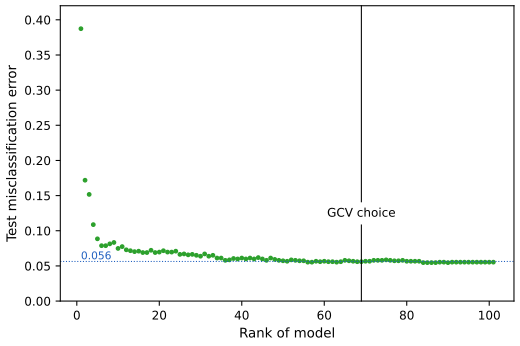
fig_9_12, spam_mars, MARS. Reproduces Hastie, Tibshirani and Friedman (2009), Figure 9.12. Download: PDF · SVGThe book reports a plateau at about 5.5% and a GCV choice of 60 terms. The leading interactions it found, (ch$, remove), (ch$, free) and (hp, CAPTOT), are matched here by (ch$, remove), (ch$, free) and (hp, CAPMAX), followed by several products with hp. On the untransformed inputs the same procedure levels off higher, at about 7%, with GCV choosing 52 terms (test error 6.2%). As in the book, the interactions bring no improvement over the additive model (5.5%).
9.4.2 Example (Simulated Data)
pp. 327–328 Three scenarios with \(N=100\), inputs and errors independent standard normal. Scenario 1 (tensor product):
\[ Y=(X_1-1)_++(X_1-1)_+\cdot(X_2-0.8)_++0.12\cdot\varepsilon, \tag{9.21} \]with a signal-to-noise ratio of about 5; scenario 2 is the same with 18 extra inputs unrelated to \(Y\) (\(p=20\)); scenario 3 has the structure of a neural network:
\[ \ell_1=X_1+X_2+X_3+X_4+X_5,\quad\ell_2=X_6-X_7+X_8-X_9+X_{10},\quad\sigma(t)=\frac1{1+e^{-t}},\quad Y=\sigma(\ell_1)+\sigma(\ell_2)+0.12\cdot\varepsilon. \tag{9.22} \]With \(\mu(x)\) the true mean, and averages over 1000 test inputs,
\[ \MSE_0=\ave_{x\in\text{Test}}(\bar y-\mu(x))^2,\qquad\MSE=\ave_{x\in\text{Test}}(\hf(x)-\mu(x))^2, \tag{9.23} \] \[ R^2=\frac{\MSE_0-\MSE}{\MSE_0}. \tag{9.24} \]| Scenario | book: mean (SE), 5 runs | here: mean (SE), first 5 runs | here: median, 50 runs | here: mean, 50 runs | runs with R2 > 0.9 |
|---|---|---|---|---|---|
| 1: tensor product, \(p=2\) | 0.97 (0.01) | 0.83 (0.11) | 0.92 | -1.39 | 28 of 50 |
| 2: tensor product, \(p=20\) | 0.96 (0.01) | 0.56 (0.07) | 0.65 | -5.01 | 4 of 50 |
| 3: neural network | 0.79 (0.01) | 0.66 (0.05) | 0.65 | 0.61 | 0 of 50 |
Table 9.4, reproduced: proportional decrease in model error \(R^2\) (9.24) of MARS (products of degree at most 2, forward pass to \(\max(21,2p+1)\) terms, GCV with \(c=3\)) in the three scenarios; 50 simulations with numpy.random.default_rng(2009). Code: mars_scenarios, table_9_4. Reproduces Hastie, Tibshirani and Friedman (2009), Table 9.4.
The ordering of the scenarios agrees with the book only in part, and the levels are lower. In most runs of scenario 1 MARS finds the hinge at 1 in \(X_1\) (median \(R^2\) 0.92); when it misses the product term, which is nonzero for only about 3 of the 100 points, \(R^2\) drops to about 0.88. The 18 useless inputs of scenario 2 hurt much more than the book reports: with 20 inputs and 100 points the forward pass finds spurious products, and GCV with \(c=3\) does not always remove them. Finally, the mean over many runs is dominated by a few disasters (the worst \(R^2\) values are -86 and -277): a product of hinges fitted to a handful of points grows quadratically outside them, and test inputs from a Gaussian do fall outside. An independent implementation of MARS gives similar values on data simulated in the same way, so these are properties of the method in this small-sample setting rather than of our code; the book's numbers are best read as typical runs.
9.4.3 Other Issues
pp. 328–329 MARS for classification. Two classes: code 0/1 and regress, as above. \(K\) classes: a multi-response MARS on the indicator responses with a common basis (subject to the masking problems of Section 4.2 of the book), or the optimal scoring of Section 12.5; PolyMARS (Stone et al., 1997) grows the basis with a quadratic approximation to the multinomial log-likelihood and refits by maximum likelihood. Mixed inputs. A categorical input contributes, for each two-group partition of its levels, a pair of indicator functions, treated like any other pair.
Result 9.12 (MARS with step functions is CART) pp. 328–329
Change MARS in two ways: (i) use the step functions \(I(x-t\gt0)\) and \(I(x-t\le0)\) instead of the hinges; (ii) when a term is multiplied by a candidate pair it is replaced by the two products and is no longer available as a parent. Then the forward pass is CART's tree-growing algorithm: the terms are the indicators of the leaves, and adding a pair is splitting a leaf.
Proof
By induction the terms are indicators of disjoint boxes covering the input space (initially the single box with indicator 1). Multiplying the indicator of a box \(R\) by \(I(x_j\gt t)\) and \(I(x_j\le t)\) gives the indicators of the two halves of \(R\); by (ii) the term for \(R\) is replaced, so the terms remain the indicators of a partition, refined by splitting \(R\). Least squares on indicators of disjoint boxes fits the box means (Result 9.4), so the RSS of the model is the sum over boxes of within-box sums of squares, and the decrease from splitting \(R\) at \((j,t)\) is exactly the decrease in (9.13) for that node. Choosing the best (parent, input, knot) is therefore choosing the best leaf and split, CART's greedy step (grown best-first). Rule (ii) means a box can be split only once, which is what gives the binary-tree representation; it is also what stops CART from adding a second, additive effect to a box that has already been split, the difficulty of Filling the gap 9.10. MARS drops both changes. ∎
9.5 Hierarchical Mixtures of Experts
pp. 329–332 The hierarchical mixture of experts (HME; Jordan and Jacobs, 1994) is a tree with soft splits: at each internal node an observation goes left or right with probabilities that depend on a linear combination of its inputs, and each leaf fits a linear (or logistic) model rather than a constant. The internal nodes are gating networks, the leaves experts (Figure 9.13 of the book is a diagram of a two-level HME and is not redrawn). Let the first element of \(x\) be 1.
See also (companion course): Bayesian and Probabilistic Machine Learning, Section 14.5.3, mixtures of experts, and its mixture-of-experts demonstration.
Definition 9.5 (a two-level HME) pp. 330–331, (9.25)–(9.30)
The top gating network has outputs
\[ g_j(x,\gamma_j)=\frac{e^{\gamma_j^\T x}}{\sum_{k=1}^Ke^{\gamma_k^\T x}},\qquad j=1,2,\dots,K, \tag{9.25} \]a soft \(K\)-way split; letting one coefficient of \(\gamma_j\) go to \(\pm\infty\) (with \(K=2\)) gives a hard split on that input. The second-level gates are
\[ g_{\ell\given j}(x,\gamma_{j\ell})=\frac{e^{\gamma_{j\ell}^\T x}}{\sum_{k=1}^Ke^{\gamma_{jk}^\T x}},\qquad\ell=1,2,\dots,K, \tag{9.26} \]the probability of branch \(\ell\) given branch \(j\). Each expert has a model
\[ Y\sim\Pr(y\given x,\theta_{j\ell}), \tag{9.27} \]for regression the Gaussian linear model, with \(\theta_{j\ell}=(\beta_{j\ell},\sigma_{j\ell}^2)\),
\[ Y=\beta_{j\ell}^\T x+\varepsilon\quad\text{and}\quad\varepsilon\sim N(0,\sigma_{j\ell}^2), \tag{9.28} \]and for classification the linear logistic model
\[ \Pr(Y=1\given x,\theta_{j\ell})=\frac1{1+e^{-\theta_{j\ell}^\T x}}. \tag{9.29} \]With \(\Psi=\{\gamma_j,\gamma_{j\ell},\theta_{j\ell}\}\), the model is the mixture
\[ \Pr(y\given x,\Psi)=\sum_{j=1}^Kg_j(x,\gamma_j)\sum_{\ell=1}^Kg_{\ell\given j}(x,\gamma_{j\ell})\Pr(y\given x,\theta_{j\ell}). \tag{9.30} \]Result 9.13 (EM for the hierarchical mixture of experts) p. 331
Introduce latent indicators \(\Delta_j\) (which top branch) and \(\Delta_{\ell\given j}\) (which second-level branch). Given the current \(\Psi\), the E-step computes for each observation the posterior probabilities of the paths,
\[ h_{j\ell,i}=\frac{g_j(x_i)\,g_{\ell\given j}(x_i)\Pr(y_i\given x_i,\theta_{j\ell})}{\sum_{j',\ell'}g_{j'}(x_i)\,g_{\ell'\given j'}(x_i)\Pr(y_i\given x_i,\theta_{j'\ell'})},\qquad h_{j,i}=\sum_\ell h_{j\ell,i}. \]The M-step maximises the expected complete-data log-likelihood, which separates into: (i) for each expert, a regression with observation weights \(h_{j\ell,i}\) (weighted least squares for (9.28), with \(\hat\sigma_{j\ell}^2\) the weighted mean squared residual; weighted logistic regression for (9.29)); (ii) for the top gate, a multinomial logistic regression of the soft targets \((h_{1,i},\dots,h_{K,i})\) on \(x_i\); (iii) for gate \(j\) at the second level, a multinomial logistic regression of the soft targets \(h_{j\ell,i}/h_{j,i}\) with observation weights \(h_{j,i}\). Each EM iteration does not decrease the log-likelihood \(\sum_i\log\Pr(y_i\given x_i,\Psi)\); this remains true if the M-steps for the gates only increase, rather than maximise, their objectives (generalised EM).
Proof
The complete-data likelihood of observation \(i\), if the path \((j,\ell)\) were known, is \(g_j(x_i)g_{\ell\given j}(x_i)\Pr(y_i\given x_i,\theta_{j\ell})\), so
\[ \ell_c(\Psi)=\sum_i\sum_{j,\ell}\Delta_{j,i}\Delta_{\ell\given j,i}\big\{\log g_j(x_i)+\log g_{\ell\given j}(x_i)+\log\Pr(y_i\given x_i,\theta_{j\ell})\big\}. \]Its expectation given the data and the current parameters replaces \(\Delta_{j,i}\Delta_{\ell\given j,i}\) by its posterior probability \(h_{j\ell,i}\), which is Bayes' theorem with prior \(g_jg_{\ell\given j}\) and likelihood \(\Pr(y_i\given x_i,\theta_{j\ell})\): the E-step formula. The expectation splits into three groups of terms with disjoint parameters: \(\sum_i\sum_{j,\ell}h_{j\ell,i}\log\Pr(y_i\given x_i,\theta_{j\ell})\), which for each \((j,\ell)\) is a weighted log-likelihood of one expert; \(\sum_i\sum_jh_{j,i}\log g_j(x_i)\), the log-likelihood of a multinomial logistic regression with soft responses \(h_{j,i}\); and \(\sum_i\sum_jh_{j,i}\sum_\ell(h_{j\ell,i}/h_{j,i})\log g_{\ell\given j}(x_i)\), for each \(j\) a weighted multinomial logistic log-likelihood. For the Gaussian expert, maximising \(\sum_ih_{j\ell,i}\{-\tfrac12\log\sigma^2-(y_i-\beta^\T x_i)^2/(2\sigma^2)\}\) gives the weighted least-squares \(\hat\beta_{j\ell}\) and \[\hat\sigma^2_{j\ell}=\sum_ih_{j\ell,i}(y_i-\hat\beta^\T x_i)^2/\sum_ih_{j\ell,i}.\] The gate problems are concave in the \(\gamma\)'s and are solved by Newton–Raphson (IRLS). That EM increases the observed log-likelihood is the general property of EM (Section 8.5; proved in the companion course, Bayesian and Probabilistic Machine Learning, Section 9.4): \[\log\Pr(\by\given\Psi)=Q(\Psi\given\Psi^{\text{old}})-H(\Psi\given\Psi^{\text{old}})\] with \(H\) maximised at \(\Psi^{\text{old}}\), so any \(\Psi\) with \(Q(\Psi\given\Psi^{\text{old}})\ge Q(\Psi^{\text{old}}\given\Psi^{\text{old}})\) does not decrease the log-likelihood. ∎
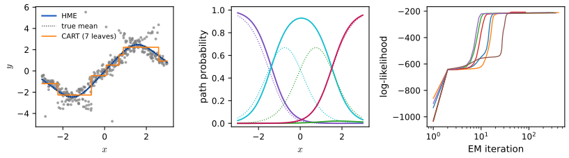
fig_9_s2, hme_fit. Download: PDF · SVGCompared with CART, the soft splits make the likelihood a smooth function of all the parameters (a tree with linear-combination splits is much harder to optimise) and capture gradual transitions, as in the figure. But there is no good method for choosing the topology of an HME: one uses a fixed tree, possibly the one CART grows, and EM can be slow and has local maxima. Research on HMEs has emphasised prediction rather than interpretation; the latent class model (Lin et al., 2000) is a one-layer relative whose classes are interpreted as groups of subjects.
9.6 Missing Data
pp. 332–333 Let \(\by\) be the response, \(\bX\) the \(N\times p\) inputs, \(\bX_{\text{obs}}\) the observed entries, \(\mathbf Z=(\by,\bX)\), \(\mathbf Z_{\text{obs}}=(\by,\bX_{\text{obs}})\), and \(\mathbf R\) the indicator matrix with \(r_{ij}=1\) if \(x_{ij}\) is missing.
Definition 9.6 (missing at random, missing completely at random) p. 332, (9.31)–(9.32)
The data are missing at random (MAR) if the distribution of \(\mathbf R\) depends on the data only through the observed part:
\[ \Pr(\mathbf R\given\mathbf Z,\theta)=\Pr(\mathbf R\given\mathbf Z_{\text{obs}},\theta), \tag{9.31} \]and missing completely at random (MCAR) if it does not depend on the data at all:
\[ \Pr(\mathbf R\given\mathbf Z,\theta)=\Pr(\mathbf R\given\theta). \tag{9.32} \]Here \(\theta\) are the parameters of the missingness mechanism. MCAR implies MAR. A measurement not taken because the patient was too sick is neither.
Result 9.14 (under MAR the mechanism can be ignored in likelihood inference) p. 332
Suppose the data have density \(\Pr(\mathbf Z\given\phi)\) and the mechanism \(\Pr(\mathbf R\given\mathbf Z,\theta)\), with \(\phi\) and \(\theta\) distinct (variation independent). Under MAR the likelihood of what is observed, \((\mathbf Z_{\text{obs}},\mathbf R)\), factorises as
\[ \Pr(\mathbf Z_{\text{obs}},\mathbf R\given\phi,\theta)=\Pr(\mathbf R\given\mathbf Z_{\text{obs}},\theta)\cdot\Pr(\mathbf Z_{\text{obs}}\given\phi), \]so maximum likelihood for \(\phi\) can use \[\Pr(\mathbf Z_{\text{obs}}\given\phi)=\int\Pr(\mathbf Z\given\phi)\,\d\mathbf Z_{\text{mis}}\] and ignore the mechanism. Analyses that use only the complete cases, or impute without modelling the dependence on the observed data, need MCAR in general.
Proof, and an example of what MAR does not buy
Integrate the missing values out of the joint density: \[\Pr(\mathbf Z_{\text{obs}},\mathbf R\given\phi,\theta)=\int\Pr(\mathbf R\given\mathbf Z,\theta)\Pr(\mathbf Z\given\phi)\,\d\mathbf Z_{\text{mis}}.\] Under MAR the first factor equals \(\Pr(\mathbf R\given\mathbf Z_{\text{obs}},\theta)\), which does not involve \(\mathbf Z_{\text{mis}}\) and comes out of the integral; what remains is \(\Pr(\mathbf Z_{\text{obs}}\given\phi)\). As a function of \(\phi\), the likelihood is proportional to \(\Pr(\mathbf Z_{\text{obs}}\given\phi)\) whatever \(\theta\) is, so it has the same maximiser (Rubin, 1976; Little and Rubin, 2002). Example. Let \(Y=1+2X+\varepsilon\) with \(X,\varepsilon\) standard normal, and let \(Y\) be missing with probability \(\sigma(2X)\), a MAR mechanism. With 20,000 cases the mean of the observed \(y\) is far from \(\E Y=1\) (the cases with large \(x\), hence large \(y\), are missing more often), whereas regressing \(y\) on \(x\) in the complete cases and averaging the predictions over all \(x\) gives about 1: the likelihood of \(Y\given X\) is unaffected by MAR missingness in \(Y\), but naive summaries are not.
The mechanism can sometimes be diagnosed: for a categorical input, code "missing" as a level and see whether it predicts the response. Assuming MCAR, one can (1) discard incomplete observations, if there are few; (2) let the learning method handle them (surrogate splits in CART, similar devices in MARS and PRIM; in a GAM, observations missing \(x_j\) are left out when smoothing against \(x_j\) and their \(\hf_j\) is set to zero, which, since each \(\hf_j\) has mean zero, is mean imputation of that term); or (3) impute before training, with the mean or median of the feature, or better with a predictive model of each feature given the others (a flexible one, such as CART, which itself copes with missing values), and then, to account for the uncertainty of imputation, with multiple imputation: several imputed training sets, a fit to each, and the spread of the results (with CART as the engine, by sampling from the values in the terminal node).
9.7 Computational Considerations
p. 334 Additive models: \(m\) backfitting cycles of \(p\) one-dimensional smoothers; with smoothing splines, an initial sort (\(N\log N\) per input) and \(O(N)\) per fit, \(pN\log N+mpN\) in all; \(m\) is usually below 20 for weakly correlated inputs (Filling the gap 9.2). Trees: \(pN\log N\) for the initial sorts and, in a balanced tree, about as much again for the split searches (each level of the tree scans every input over all \(N\) observations once, Result 9.4); splits near the ends of the ranges can make the depth, and the cost, as large as \(N^2p\). MARS: the book counts \(Nm^2+pmN\) operations to add a term to a model of \(m\) terms, \(NM^3+pM^2N\) for \(M\) terms. With the one-pass knot search of Result 9.10, each (parent, input) pair costs \(O(Nm)\) and there are up to \(m\) parents and \(p\) inputs, so a step costs \(O(pNm^2)\); the 101-term spam fit (3065 observations, 57 inputs) takes about two minutes. HME: each M-step is cheap (\(Np^2\) for each regression, \(Np^2K^2\) for a \(K\)-class logistic regression), but EM may need many iterations.
Exercises
pp. 335–336 Each exercise is restated in my own words, followed by a worked solution (open it with its bar).
Exercise 9.1. Show that a smoothing-spline fit of \(y_i\) on \(x_i\) preserves the linear part of the fit: if \(y_i=\hat y_i+r_i\), with \(\hat y_i\) the least-squares straight-line fit, and \(\bS\) is the smoother matrix, then \(\bS\by=\hat\by+\bS\br\). Show the same for local linear regression (Section 6.1.1), and argue from this that the centring step in Algorithm 9.1 is unnecessary.
Solution
Both smoothers reproduce straight lines: \(\bS\bv=\bv\) whenever \(v_i=a+bx_i\). For the smoothing spline, \(\bS=(\bI+\lambda\bK)^{-1}\) and \(\bK\bv=\bzero\) because a straight line has zero second derivative, so the penalty vanishes and the line is its own fit (eigenvalue 1, Result 5.7); for local linear regression the equivalent kernel satisfies \(\sum_il_i(x_0)=1\) and \(\sum_i(x_i-x_0)l_i(x_0)=0\) (Result 6.2), so \(\sum_il_i(x_0)(a+bx_i)=a+bx_0\). Since \(\hat\by\) is a line, linearity gives \(\bS\by=\bS\hat\by+\bS\br=\hat\by+\bS\br\).
The centring step. In backfitting the partial residual has mean zero when \(\hat\alpha=\bar y\) and the other terms have mean zero; write it as \(\hat\by+\br\) with \(\hat\by\) its fitted line (which has the same mean, zero) and \(\br\) the residual (mean zero). Then \(\bS(\hat\by+\br)=\hat\by+\bS\br\), and the fit has mean zero exactly when \(\bone^\T\bS\br=0\). For the smoothing spline \(\bS\) is symmetric and \(\bS\bone=\bone\), so \(\bone^\T\bS\br=(\bS\bone)^\T\br=\bone^\T\br=0\): the centring step is indeed unnecessary (up to rounding). For local linear regression the argument fails, because its smoother matrix is not symmetric and \(\bone^\T\bS\ne\bone^\T\) in general: the column sums of \(\bS\) are not one. In a small example (60 points with a skewed design, tri-cube nearest-neighbour span 0.5) a mean-zero response gave a local linear fit with mean 0.025, so the centring step is needed there; the conclusion of the exercise holds for symmetric smoothers that reproduce constants, not for every smoother that preserves lines.
Exercise 9.2. A Gauss–Seidel method solves \(\bA\bz=\bb\) by solving the \(j\)-th equation for \(z_j\) with the other components at their current values, for \(j=1,\dots,k\), repeatedly. (a) For an additive model with linear smoothers \(\bS_j\), show that backfitting is block Gauss–Seidel for the system (9.33). (b) With two symmetric smoothers \(\bS_1,\bS_2\) whose eigenvalues lie in \([0,1)\), show that backfitting converges from any starting values and give the limits.
Solution
(a) Result 9.2(a): block row \(j\) of (9.33) solved for \(\bf_j\) is \(\bf_j=\bS_j(\by-\sum_{k\ne j}\bf_k)\), the backfitting update.
(b) One cycle is \(\bf_1^{(k+1)}=\bS_1(\by-\bf_2^{(k)})\), \(\bf_2^{(k+1)}=\bS_2(\by-\bf_1^{(k+1)})\). Substituting the second equation of cycle \(k\) into the first of cycle \(k+1\),
\[ \bf_1^{(k+1)}=\bS_1(\bI-\bS_2)\by+\bS_1\bS_2\bf_1^{(k)}. \]A symmetric matrix with eigenvalues in \([0,1)\) has spectral norm below 1, so \(\|\bS_1\bS_2\|\le\|\bS_1\|\|\bS_2\|\lt1\): the map is a contraction, \(\bI-\bS_1\bS_2\) is invertible, and \(\bf_1^{(k)}\) converges geometrically, from any start, to the unique fixed point
\[ \bf_1^{(\infty)}=(\bI-\bS_1\bS_2)^{-1}\bS_1(\bI-\bS_2)\by,\qquad\bf_2^{(\infty)}=\bS_2(\by-\bf_1^{(\infty)})=(\bI-\bS_2\bS_1)^{-1}\bS_2(\bI-\bS_1)\by. \]For the second form, multiply \(\bS_2(\by-\bf_1^{(\infty)})\) by \(\bI-\bS_2\bS_1\) and use the fixed-point equation \(\bf_1^{(\infty)}=\bS_1(\bI-\bS_2)\by+\bS_1\bS_2\bf_1^{(\infty)}\) to get \(\bS_2(\bI-\bS_1)\by\). The error of \(\bf_1\) is multiplied by \(\bS_1\bS_2\) at each cycle (Filling the gap 9.2). A computation with random symmetric smoothers confirms the limits to \(10^{-9}\). Smoothing splines have eigenvalue 1 on lines and constants, outside the hypothesis; there the fitted values still converge but the functions are determined only up to the trade of linear parts described in Result 9.1(d).
Exercise 9.3. Run backfitting with orthogonal projections \(\bS_j=\bP_j\) onto the column spaces of matrices \(\bD_j\), and let \(\bD=(\bD_1,\dots,\bD_p)\). Show that the estimating equations (9.33) are equivalent to the least-squares normal equations \(\bD^\T\bD\boldsymbol\beta=\bD^\T\by\).
Solution
(\(\Leftarrow\)) Let \(\boldsymbol\beta=(\boldsymbol\beta_1,\dots,\boldsymbol\beta_p)\) solve the normal equations and put \(\bf_j=\bD_j\boldsymbol\beta_j\). The \(j\)-th block of the normal equations is \(\bD_j^\T(\by-\sum_k\bf_k)=\bzero\), so \(\bP_j(\by-\sum_k\bf_k)=\bzero\). Since \(\bf_j\) lies in the column space, \(\bP_j\bf_j=\bf_j\), and the equation becomes \(\bf_j+\bP_j\sum_{k\ne j}\bf_k=\bP_j\by\), block row \(j\) of (9.33). (\(\Rightarrow\)) If \((\bf_1,\dots,\bf_p)\) solves (9.33), then \(\bf_j=\bP_j(\by-\sum_{k\ne j}\bf_k)\) lies in the column space of \(\bD_j\), so \(\bf_j=\bD_j\boldsymbol\beta_j\) for some \(\boldsymbol\beta_j\), and (9.33) gives \(\bP_j(\by-\sum_k\bf_k)=\bzero\), i.e. \(\bD_j^\T(\by-\bD\boldsymbol\beta)=\bzero\) for all \(j\): the normal equations. Hence backfitting with projections converges to the least-squares fit of \(\by\) on all the columns together (the column space \(V=\mathcal L_{\rm col}(\bS_1)\oplus\dots\oplus\mathcal L_{\rm col}(\bS_p)\)); each update is the exact minimisation of the RSS over one block, and the code confirms that the limit is the least-squares fit to \(10^{-9}\).
Exercise 9.4. Use the same symmetric smoother \(\bS\), with eigenvalues in \([0,1)\), for both terms of a two-term additive model (the two inputs are identical). Show that the backfitting residual converges to \((\bI+\bS)^{-1}(\bI-\bS)\by\) and that the residual sum of squares converges upward. Can it converge upward in less structured situations? Compare the fit with that of a single term fitted by \(\bS\).
Solution
Write \(\bS=\mathbf U\diag(\rho_k)\mathbf U^\T\) and work with one eigen-coordinate, \(a=\bu_k^\T\by\), \(\rho=\rho_k\in[0,1)\), and coordinates \(u,v\) of \(\bf_1,\bf_2\). Backfitting from zero is \(u\leftarrow\rho(a-v)\), \(v\leftarrow\rho(a-u)\). The fixed point is \(u=v=\rho a/(1+\rho)\), with residual \(a-2\rho a/(1+\rho)=a(1-\rho)/(1+\rho)\): in matrix form \((\bI+\bS)^{-1}(\bI-\bS)\by\). Convergence. With \(d_k=u_k-\rho a/(1+\rho)\) after cycle \(k\), \(v_k=\rho(a-u_k)\) and \(u_{k+1}=\rho(a-v_k)\) give \(d_{k+1}=\rho^2d_k\); from \(u_1=\rho a\), \(d_1=\rho^2a/(1+\rho)\). Upward. The residual at the end of cycle \(k\) is \[a-u_k-v_k=(1-\rho)(a-u_k)=(1-\rho)\{a/(1+\rho)-d_k\},\] and \(d_k=\rho^{2(k-1)}d_1\) has the sign of \(a\) and shrinks monotonically, so the residual coordinate grows in absolute value, monotonically, towards \(a(1-\rho)/(1+\rho)\); summing squares over the coordinates, the RSS at the end of each cycle increases to \(\sum_ka_k^2(1-\rho_k)^2/(1+\rho_k)^2\). (Within a cycle it zigzags: after the first update of a cycle it is above its limit.) Less structured cases. Yes: what backfitting decreases at every step is the penalised criterion (9.7) (Result 9.2(b)), not the RSS; whenever the terms compete for the same directions, the first cycle overfits them greedily and later cycles trade some fit for a smaller penalty, so the RSS can rise. Only for projections, where there is no penalty, is backfitting coordinate descent on the RSS itself, and then the RSS never increases. Comparison. The two-term fit is \(\by-(\bI+\bS)^{-1}(\bI-\bS)\by=2\bS(\bI+\bS)^{-1}\by\), a smoother with eigenvalues \(2\rho_k/(1+\rho_k)\ge\rho_k\): it smooths less than \(\bS\) alone (the smallest eigenvalues are roughly doubled, the eigenvalues near 1 barely change). On the ozone data with temperature as both inputs and \(\Tr\bS=5\), the two-term fit has \(\sum_k2\rho_k/(1+\rho_k)=5.78\) degrees of freedom; its RSS at the end of each cycle rises to 32.43, below the single fit's 32.98 (Figure 9.S4, right).
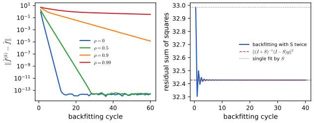
Figure 9.S4 (supplementary, Exercises 9.2 and 9.4). Left: distance of the backfitting iterate from its limit, for two smoothing-spline terms (\(\Tr\bS_j=5\)) in inputs with correlation \(\rho\); the error shrinks by about 0.065, 0.32, 0.82 and 0.98 per cycle for \(\rho=0\), 0.5, 0.9, 0.99 (Filling the gap 9.2). Right: backfitting the cube root of ozone with the same smoother (\(\Tr\bS=5\)) on temperature for both terms: the RSS after each half cycle, its limit \(\|(\bI+\bS)^{-1}(\bI-\bS)\by\|^2\) and the RSS of a single fit. Code: fig_9_s4. Download: PDF · SVG▶ DemoThe same smoother twice (Exercise 9.4)Temperature entered twice: the end-of-cycle RSS creeps up to its limit.Exercise 9.5. Degrees of freedom of a tree. With \(\E y_i=f(x_i)\), \(\Var y_i=\sigma^2\), define the degrees of freedom of a fit \(\by\mapsto\hat\by\) as \(\sum_i\Cov(y_i,\hat y_i)/\sigma^2\). For a regression tree on \(X_1,\dots,X_p\): (a) give a rough formula in terms of the number of leaves \(m\); (b)–(c) with 100 fixed observations of ten independent standard Gaussian inputs and pure-noise standard Gaussian responses, fit trees with 1, 5 and 10 leaves to ten simulated response vectors and estimate the degrees of freedom; (d) compare; (e) suggest an approximate smoother matrix \(\bS\) for a tree, compute it and compare \(\Tr\bS\).
Solution
(a) If the partition were fixed in advance, \(\hat\by=\bP\by\) with \(\bP\) the projection onto the \(m\) leaf indicators, and \(\df=\Tr\bP=m\). That is the naive answer. (b)–(c) Trees of exactly \(m\) leaves were grown best-first (split the leaf with the largest decrease in RSS; children of at least 5 observations), and \(\df\) was estimated by \(\sum_i\widehat{\Cov}(y_i,\hat y_i)\) over the simulated responses (
tree_df_simulation). With ten simulations: 0.71, 26.3 and 44.5 for \(m=1,5,10\); with 400 simulations: 0.96, 29.0 and 49.7 (the one-leaf tree is the mean, with \(\df=1\) exactly). (d) The search for splits adapts to the noise: a tree with 5 leaves uses about 29 degrees of freedom, six times the naive count, because each split is chosen from about \(10\times99\) candidates to fit the particular response. The excess per split is about \(29/4\approx7\) for the first few splits and falls as the leaves get small (20 leaves: about 61). Ten simulations give a rough but already clear picture. (e) Two approximate smoother matrices: the projection onto the leaves of the tree fitted to \(\by\), which ignores the search and has trace \(m\); and a perturbation estimate (Ye, 1998): refit the tree to \(\by+\boldsymbol\delta\) for many small perturbations \(\boldsymbol\delta\sim N(\bzero,\tau^2\bI)\) and take \(\hat S_{ij}\) as the slope of the regression of \(\hat y_i\) on \(\delta_j\). With \(\tau=0.5\) and 200 perturbations its trace is 1.2, 30.3 and 49.6 for \(m=1,5,10\), agreeing with the covariance definition, because the slope of \(\hat y_i\) on \(\delta_i\) measures exactly how much \(\hat y_i\) follows its own response, through the choice of splits as well as through the leaf means.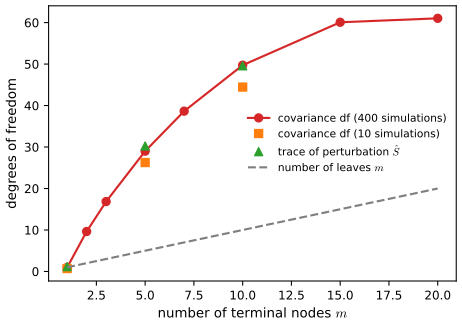
Figure 9.S3 (supplementary, Exercise 9.5). Degrees of freedom of regression trees with \(m\) leaves fitted to pure noise (100 observations, ten Gaussian inputs): covariance estimate from 400 and from 10 simulated responses, trace of the perturbation estimate of \(\bS\), and the naive count \(m\). Code: fig_9_s3,tree_df_simulation,tree_df_ye. Download: PDF · SVGExercise 9.6. For the ozone data of Figure 6.9: (a) fit an additive model to the cube root of ozone concentration as a function of temperature, wind speed and radiation, and compare with the trellis display of Figure 6.9; (b) fit trees, MARS and PRIM to the same data and compare with (a) and with Figure 6.9.
Solution
(a) The 111 days of the New York ozone data, with cube-root ozone as response, fitted by backfitting (Algorithm 9.1) with three exact smoothing splines of \(\Tr\bS_j=4\) (three degrees of freedom beyond the constant each); it converged in 20 cycles and explains 75.9% of the variance (Figure 9.S1). Cube-root ozone rises steadily with temperature (by about 1.5 units, i.e. ozone roughly triples, over 60–95°F), falls with wind speed (steeply up to about 10 mph and then more slowly) and rises with radiation up to about 250 langleys before flattening. The trellis display of Figure 6.9 conditions on temperature and wind and shows ozone against radiation in each panel: the radiation effect has a similar rising, flattening shape in each panel, with the level shifting with temperature and wind, which is what an additive model says. The trellis panels also suggest that the radiation effect is steeper on hot, calm days, an interaction the additive model cannot express.
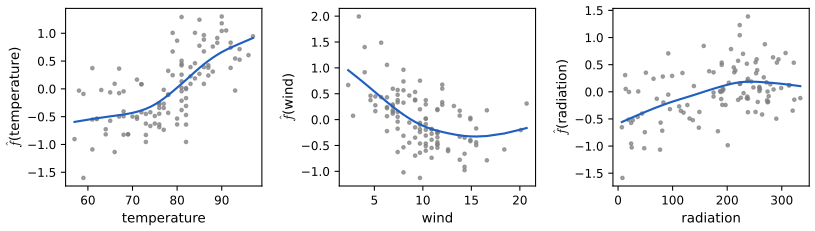
Figure 9.S1 (supplementary, Exercise 9.6). The additive model for the cube root of ozone: fitted functions with partial residuals \(\hf_j(x_{ij})+r_i\). Code: fig_9_s1,ozone_additive. Download: PDF · SVG(b) Ten-fold cross-validated mean squared error on the cube-root scale (the variance of the response is 0.786): linear model 0.269; additive model of (a) 0.262; regression tree 0.236 (grown to nodes of at least 10 days, pruned by cost complexity with the size chosen by cross-validation, 11 leaves); MARS additive 0.232; MARS with pairwise products 0.244. All the flexible fits beat the linear model by a similar margin and differ from one another by less than their sampling error with 111 days. MARS with products, fitted to all the data, keeps the terms \((\mathrm{temp} - 73)_+\), \((9.7 - \mathrm{wind})_+\cdot (91 - \mathrm{temp})_+\), \((225 - \mathrm{rad})_+\cdot (\mathrm{temp} - 67)_+\), \((73 - \mathrm{temp})_+\cdot (12 - \mathrm{wind})_+\): an effect of temperature above 73°F and interactions of temperature with wind and with radiation, the same kind of interaction that the trellis display suggests. PRIM (\(\alpha=0.1\)) looking for high ozone peels down to a box of about 20% of the days, here 22 days with temperature from 79 to 94°F, wind at most 8.6 mph and radiation from 167 to 272 langleys, where the mean cube-root ozone is 4.43 (about 87 ppb, against a mean of 42 ppb over all days): hot, calm, sunny days, the corner of the trellis display where ozone is highest. The tree splits first on temperature (at 82.5°F) and then on temperature, wind and radiation.
Demonstrations for this chapter
Each demonstration runs in the browser on the course's data files and links back to these notes. The ▶ Demo boxes above open them already set to the case under discussion.
| Demonstration | What you can see | Sections and results |
|---|---|---|
| Backfitting step by step | An additive model of smoothing-spline terms fitted one smoother update at a time: the partial residuals being smoothed, every function, the RSS and the penalised criterion after each update, the degrees of freedom of each term; the ozone data, two simulated inputs with any correlation, and the same input entered twice. Presets: 1 ozone, one update at a time; 2 ozone, converged; 3 correlated inputs; 4 the same smoother twice; 5 one df per term (a linear model). | 9.1.1; Algorithm 9.1, Result 9.2, Filling the gap 9.2, Exercise 9.4 |
| Growing and pruning a classification tree | The spam tree grown in the browser with deviance or Gini, the weakest-link sequence, the subtree \(T_\alpha\) for any \(\alpha\), its training, test and 10-fold cross-validated error, the one-standard-error rule, and losses on the email class. Presets: 1 the pruning sequence; 2 cross-validation; 3 the 17-leaf tree; 4 weight 5 on email; 5 Gini. | 9.2.2–9.2.5; Results 9.5–9.7, Filling the gap 9.5 |
| MARS: forward and backward passes | MARS on two inputs: each forward step adds the best product of a term and a reflected pair; the fitted surface, the terms, the backward deletion sequence and the GCV curve with the knot cost \(c\) adjustable; tensor-product data (9.21) and the ozone data. Presets: 1 forward pass step by step; 2 full fit and GCV; 3 additive only; 4 ozone; 5 no knot cost. | 9.4; Results 9.10–9.12, Filling the gap 9.12 |
Related demonstrations in the companion course: the trees and committees demonstration and the mixture-of-experts demonstration. In this course, the smoothing-spline demonstration of Chapter 5 shows the one-dimensional smoother that backfitting cycles over. The Python code that produces every figure of this page is code/ch09_additive_models_trees.py (see the code index).
References
- Hastie, T., Tibshirani, R. and Friedman, J. (2009). The Elements of Statistical Learning: Data Mining, Inference, and Prediction, 2nd edition. Springer, New York. Chapter 9, pp. 295–336. hastie.su.domains/ElemStatLearn.
- Breiman, L., Friedman, J., Olshen, R. and Stone, C. (1984). Classification and Regression Trees. Wadsworth, Belmont, California.
- Buja, A., Hastie, T. and Tibshirani, R. (1989). Linear smoothers and additive models (with discussion). The Annals of Statistics, 17(2), 453–555.
- Fisher, W. D. (1958). On grouping for maximum homogeneity. Journal of the American Statistical Association, 53(284), 789–798.
- Friedman, J. H. (1991). Multivariate adaptive regression splines (with discussion). The Annals of Statistics, 19(1), 1–141.
- Friedman, J. H. and Fisher, N. I. (1999). Bump hunting in high-dimensional data. Statistics and Computing, 9(2), 123–143.
- Hanley, J. A. and McNeil, B. J. (1982). The meaning and use of the area under a receiver operating characteristic (ROC) curve. Radiology, 143(1), 29–36.
- Hastie, T. and Tibshirani, R. (1990). Generalized Additive Models. Chapman and Hall, London.
- Hyafil, L. and Rivest, R. L. (1976). Constructing optimal binary decision trees is NP-complete. Information Processing Letters, 5(1), 15–17.
- Jacobs, R. A., Jordan, M. I., Nowlan, S. J. and Hinton, G. E. (1991). Adaptive mixtures of local experts. Neural Computation, 3(1), 79–87.
- Jordan, M. I. and Jacobs, R. A. (1994). Hierarchical mixtures of experts and the EM algorithm. Neural Computation, 6(2), 181–214.
- Lin, Y. and Zhang, H. H. (2006). Component selection and smoothing in multivariate nonparametric regression. The Annals of Statistics, 34(5), 2272–2297.
- Little, R. J. A. and Rubin, D. B. (2002). Statistical Analysis with Missing Data, 2nd edition. Wiley, New York.
- Quinlan, J. R. (1993). C4.5: Programs for Machine Learning. Morgan Kaufmann, San Mateo, California.
- Ravikumar, P., Liu, H., Lafferty, J. and Wasserman, L. (2008). SpAM: sparse additive models. In Advances in Neural Information Processing Systems 20, 1201–1208.
- Ripley, B. D. (1996). Pattern Recognition and Neural Networks. Cambridge University Press.
- Rubin, D. B. (1976). Inference and missing data. Biometrika, 63(3), 581–592.
- Stone, C. J., Hansen, M. H., Kooperberg, C. and Truong, Y. K. (1997). Polynomial splines and their tensor products in extended linear modeling (with discussion). The Annals of Statistics, 25(4), 1371–1470.
- Ye, J. (1998). On measuring and correcting the effects of data mining and model selection. Journal of the American Statistical Association, 93(441), 120–131.
The numerical statements in the text (the agreement of the additive logistic fit and its test errors with an independent implementation, the solution of the normal equations (9.33) by backfitting, the closed forms of Exercises 9.2–9.4, the weakest-link sequence against an exhaustive search over subtrees, the ordering trick, the knot scan and deletion formula of MARS, the monotonicity of EM, and the corrections to Table 9.1, Figure 9.5 and Exercise 9.1) were confirmed numerically.