Trees, Forests, Bagging, and Boosting
A decision tree cuts the input space into boxes by a greedy sequence of axis-parallel threshold questions and predicts a constant (a class distribution or a mean) in each box. It is cheap, readable and invariant to monotone transformations of the inputs, but it is a high-variance estimator: delete one observation and the tree can change completely. The chapter turns that weakness into a strength in two ways. Averaging many trees fitted to bootstrap samples (bagging) and decorrelating them by letting every split see only a few random features (random forests) reduce the variance and leave the bias alone. Fitting trees one after another, each to what the current ensemble still gets wrong (boosting), reduces the bias; AdaBoost, LogitBoost, gradient boosting and XGBoost are the same additive model fitted by exponential loss, Newton steps on the log loss, functional gradient descent and a regularised second-order expansion. The notes prove every statement the book leaves as "it can be shown" or "see the literature", and check the claims on the iris petals, a two-moons simulation, a one-dimensional regression problem and the 4601 spam e-mails.
Ch. 1 Introduction Ch. 2 Univariate probability Ch. 3 Multivariate probability Ch. 4 Statistics Ch. 5 Decision theory Ch. 6 Information theory Ch. 7 Linear algebra Ch. 8 Optimisation Ch. 9 Discriminant analysis Ch. 10 Logistic regression Ch. 11 Linear regression Ch. 12 GLMs Ch. 13 Networks for tabular data Ch. 14 Networks for images Ch. 15 Networks for sequences Ch. 16 Exemplar-based methods Ch. 17 Kernel methods Ch. 18 Trees and boosting Ch. 19 Fewer labels Ch. 20 Dimensionality reduction Ch. 21 Clustering Ch. 22 Recommender systems Ch. 23 Graph embeddings
How to read these notes
They follow the book. Sections carry the book's numbers (18.1.2, 18.5.3, ...) and equations the book numbers keep their numbers, e.g. \((18.30)\); equations without a number are steps the book skips. The draft of the chapter ends with Section 18.6 and has no exercises, so Section 18.7 is a set of problems of my own, in the style of the other chapters, each with a full solution.
Filling the gaps. Wherever the book writes "it can be shown", leaves a step to the reader, or quotes a result from the literature, an orange Filling the gap box gives the full argument. Proofs start hidden: open one with its bar, or use the buttons below.
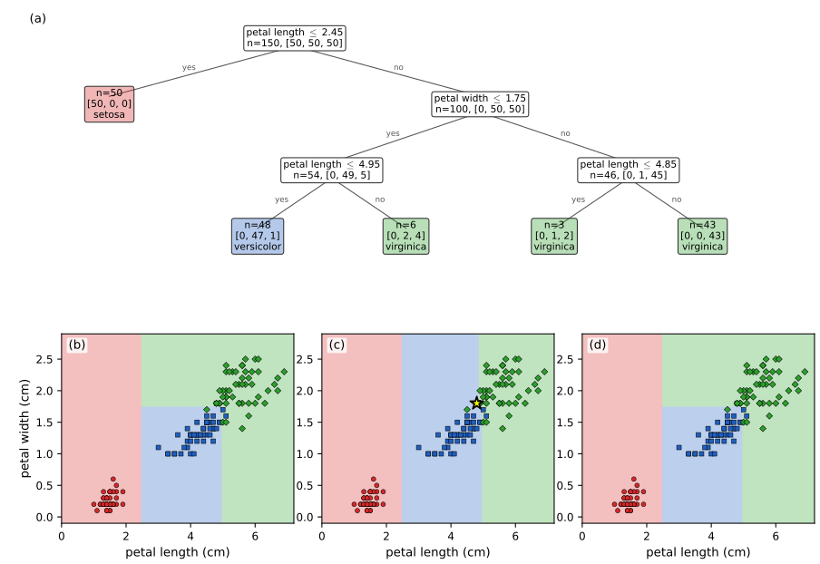
Figures and demonstrations. Every computed figure is reproduced by the Python code; Figure 18.2 (a hand-drawn set of shapes with a hypothetical tree) is not reproduced. Figure 18.1 is redrawn from the thresholds in the text. The book's iris tree of Figure 18.3 has depth 2; I use depth 3 because at depth 2 no single deleted flower moves the partition by more than 2.2% of the plane, and say so in the caption. Figures 18.4 and 18.6 use simulated data (the book's random samples are not available); Figures 18.5, 18.9 and 18.10 use the spam data with a random split of the book's sizes, so test errors differ from the book's in the third digit. Figures named 18.S are supplementary and illustrate the gaps. The ▶ Demo boxes open an interactive demonstration set to the case being discussed.
Main reference
K. P. Murphy, Probabilistic Machine Learning: An Introduction, MIT Press (2022), Chapter 18, pages 603–623 (book page: probml.github.io/pml-book/book1.html). Section, equation, figure and table numbers below refer to this book. The explanations, derivations, figures and code are my own.
Companion courses
Trees, forests and boosting are developed in more depth, with other examples, elsewhere on this site. Where a result is proved in full there, these notes give the statement and a short sketch and link to it.
- Elements of Statistical Learning (Hastie, Tibshirani, Friedman): 9.2 tree-based methods, 8.7 bagging and 8.8 model averaging and stacking, 10.4 exponential loss and AdaBoost, 10.5 why exponential loss, 10.10 gradient boosting, 10.12 shrinkage and subsampling, 10.13 importance and partial dependence, 15.2 random forests, 15.3.1 out-of-bag samples, 15.4.1 the de-correlation effect.
- Introduction to Statistical Learning: 8.1 the basics of decision trees, 8.2.1 bagging, 8.2.2 random forests, 8.2.3 boosting.
- Bayesian and Probabilistic Machine Learning (Bishop): 14.1 Bayesian model averaging (and why a committee is not the same thing), 14.2 committees, 14.3 boosting, 14.4 tree-based models.
What this chapter adds: Murphy's notation for the greedy fit, the majority-vote calculation (18.11), the formulation of boosting as forward stagewise additive modelling with a pluggable loss, the LogitBoost and gradient-boosting algorithms in one table of losses, and the second-order regularised trees of XGBoost with their closed-form gain.
The chapter at a glance
- 18.1 A tree is a piecewise constant function with one constant per leaf (gap 18.1); the greedy split search (gap 18.2), the impurity measures (gap 18.3), why greedy growing misses XOR and how cost-complexity pruning works (gap 18.4), invariance and robustness (gap 18.5) and instability (gap 18.6).
- 18.2 Majority voting and its limit when the voters are correlated (gap 18.7); stacking and why an ensemble is not Bayes model averaging (gap 18.8).
- 18.3–18.4 Bagging: the 63% rule, variance of correlated averages, Jensen and the out-of-bag estimate (gap 18.9); random forests and the decorrelation effect (gap 18.10).
- 18.5 Forward stagewise fitting and least-squares boosting (gap 18.11); why weak learners become strong (gap 18.12); AdaBoost from exponential loss (gap 18.13); LogitBoost as Newton's method (gap 18.14); gradient boosting, Table 18.1 and the leaf values (gap 18.15, gap 18.16); XGBoost (gap 18.17).
- 18.6 Feature importance and its biases (gap 18.18); partial dependence, interactions and correlated inputs (gap 18.19).
Notation. Data \(\mathcal D=\{(\bm x_n,y_n)\}_{n=1}^N\) with \(\bm x_n\in\R^D\). A tree has regions \(R_1,\dots,R_J\) (its leaves) with outputs \(w_j\); \(\mathcal D_i\) is the set of training examples that reach node \(i\). For a classifier, \(\tilde y_n\in\{-1,+1\}\) is the signed label and \(\hat\pi_{ic}\) the proportion of class \(c\) at node \(i\). An ensemble has \(M\) members \(F_m\) (or \(B\) bootstrap trees); \(f_m\) is the ensemble after \(m\) boosting rounds. In boosting \(g_{im}\) and \(h_{im}\) are the first and second derivative of the loss with respect to \(f(\bm x_i)\) at \(f_{m-1}\). \(\sigma(a)=1/(1+e^{-a})\).
Prerequisites. Chapters 4 and 5 of the book (the bias–variance trade-off, the bootstrap, Bayes model averaging, decision theory), Chapter 10 (log loss, Newton's method for logistic regression) and Chapter 8 (gradient descent).
18.1 Classification and regression trees (CART)
p. 603 A classification and regression tree (CART; Breiman et al., 1984), also called a decision tree (Quinlan, 1986, 1993), recursively partitions the input space and fits a very simple model in each cell: a constant. The partition is described by a binary tree whose internal nodes ask "is \(x_d\le t\)?" and whose leaves are the cells. The first demonstration grows such a tree on the iris petals one split at a time.
18.1.1 Model definition
pp. 603–604 At internal node \(i\) the input \(\bm x\) is compared in one coordinate \(d_i\) with a threshold \(t_i\) and sent left if \(x_{d_i}\le t_i\) and right otherwise (categorical inputs are tested for equality with one value). The path from the root to a leaf defines a region, for example \(R_1=\{\bm x:x_1\le t_1,\ x_2\le t_2\}\) in Figure 18.1a. A regression tree is the function \[ f(\bm x;\bm\theta)=\sum_{j=1}^Jw_j\,\ind(\bm x\in R_j),\qquad w_j=\frac{\sum_{n=1}^Ny_n\ind(\bm x_n\in R_j)}{\sum_{n=1}^N\ind(\bm x_n\in R_j)}, \tag{18.2, 18.3} \] with \(\bm\theta=\{(R_j,w_j)\}_{j=1}^J\), where \(J\) is the number of leaves (the book says "nodes"; a binary tree with \(J\) leaves has \(J-1\) internal nodes, see the notes on the book). For classification a leaf stores the class distribution \(\hat\pi_{jc}=\frac1{|\mathcal D_j|}\sum_{n\in\mathcal D_j}\ind(y_n=c)\) (18.7) instead of a mean.
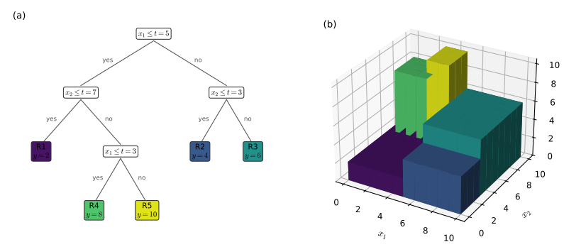
Figure 18.2 of the book (coloured shapes with a hypothetical tree) is a hand-drawn illustration with nothing computed and is not reproduced. Its message is that a node may test a categorical feature, with one branch per value (a multi-way split) or one branch for a single value against the rest (a binary split).
Filling the gap 18.1: the leaf value is the optimal constant, and counting leaves and nodes pp. 603–604, (18.2)–(18.4)
Derivation
The leaf value. Fix the regions \(R_1,\dots,R_J\). The loss (18.4) separates over leaves, \(L(\bm\theta)=\sum_j\sum_{\bm x_n\in R_j}\ell(y_n,w_j)\), so each \(w_j\) is chosen alone to minimise \(\sum_{\bm x_n\in R_j}\ell(y_n,w)\). For squared error the derivative is \(-2\sum_{\bm x_n\in R_j}(y_n-w)\), which vanishes at the sample mean, and the second derivative \(2|\mathcal D_j|>0\) makes it a minimum: this is (18.3). For classification with the log loss, \(\sum_{n\in\mathcal D_j}-\log\pi_{y_n}=-\sum_cn_{jc}\log\pi_c\) with \(n_{jc}\) the class counts; minimising over the probability vector \(\bm\pi\) in the simplex gives \(\hat\pi_c=n_{jc}/n_j\) (Lagrange multiplier: \(-n_{jc}/\pi_c+\lambda=0\), so \(\pi_c\propto n_{jc}\)), the maximum likelihood estimate (18.7). For absolute error the minimiser is a median of the \(y_n\) in the leaf (Exercise 18.7). Whatever the loss, the leaf value is a one-dimensional problem; the only hard part is finding the regions.
Leaves and nodes. In a full binary tree (every internal node has two children) let \(I\) be the number of internal nodes and \(J\) the number of leaves. Counting edges in two ways, the number of edges is \(I+J-1\) (every node but the root has one parent edge) and also \(2I\) (every internal node has two child edges), so \(J=I+1\) and the tree has \(2J-1\) nodes. Hence the sum in the importance (18.57), which runs over internal nodes, has \(J-1\) terms, which is how the book writes it. The parameters of the model are the \(J\) outputs and, for every internal node, one feature index and one threshold. The number of distinct partitions reachable with these thresholds grows exponentially with the depth, which is why exhaustive search is hopeless (finding the optimal tree is NP-complete; Hyafil and Rivest, 1976) and why a greedy rule is used. \(\square\)
18.1.2 Model fitting
pp. 605–606 The training loss \(L(\bm\theta)=\sum_n\ell(y_n,f(\bm x_n;\bm\theta))=\sum_j\sum_{\bm x_n\in R_j}\ell(y_n,w_j)\) (18.4) is not differentiable in the tree structure, and the optimal partition is NP-complete to find, so CART (Breiman et al., 1984), C4.5 and ID3 (Quinlan, 1986, 1993) grow the tree greedily, one node at a time:
- Given the examples \(\mathcal D_i\) at node \(i\), for every feature \(j\) and every candidate threshold \(t\in\mathcal T_j\) (the sorted distinct values of feature \(j\) among \(\mathcal D_i\)) form \(\mathcal D_i^L(j,t)=\{\bm x_n\in\mathcal D_i:x_{nj}\le t\}\) and \(\mathcal D_i^R(j,t)=\mathcal D_i\setminus\mathcal D_i^L\).
- Choose the pair with the smallest weighted child cost, \[ (j_i,t_i)=\argmin_{j}\ \min_{t\in\mathcal T_j}\ \frac{|\mathcal D_i^L(j,t)|}{|\mathcal D_i|}\,c\big(\mathcal D_i^L(j,t)\big)+\frac{|\mathcal D_i^R(j,t)|}{|\mathcal D_i|}\,c\big(\mathcal D_i^R(j,t)\big). \tag{18.5} \]
- Split, and call the procedure on the two children until a stopping rule applies (Section 18.1.3).
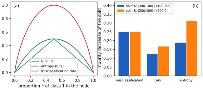
The cost \(c\) is the mean squared error \(c(\mathcal D)=\frac1{|\mathcal D|}\sum_{n\in\mathcal D}(y_n-\bar y)^2\) (18.6) for regression. For classification, with \(\hat\pi_{c}\) the class proportions in the node (18.7), it is the Gini index \[ G=\sum_{c=1}^C\hat\pi_c(1-\hat\pi_c)=1-\sum_c\hat\pi_c^2, \tag{18.8} \] the expected error rate of a rule that draws its prediction from the node's own distribution, or the entropy \(H=-\sum_c\hat\pi_c\log\hat\pi_c\) (18.9), zero for a pure node. A third choice, the misclassification rate \(1-\max_c\hat\pi_c\), is also used to prune but is a poor guide to growing, as gap 18.3 shows. Figure 18.S5 compares the three. Suárez and Lutsko (1999) replace the hard threshold by a smooth (logistic) function, giving a soft decision tree whose parameters can be fitted by gradient descent for a fixed structure.
Filling the gap 18.2: the exhaustive threshold search in one sorted pass, and the regression gain as a squared mean difference pp. 605–606, (18.5), (18.6)
Derivation
Only thresholds between consecutive values matter. For feature \(j\) the partition \(\{x_{nj}\le t\}\) changes only when \(t\) crosses a data value. So it is enough to try one \(t\) in each gap between consecutive distinct sorted values (the code uses the midpoint; the book uses the lower value with "\(\le\)", which gives the same partitions, plus a degenerate last threshold that sends everything left). With \(n\) examples at the node there are at most \(n-1\) distinct partitions per feature.
One pass. Sort the node's examples by feature \(j\). Write \(S_k\) for the vector of statistics of the first \(k\) examples in sorted order (class counts for the Gini index and entropy; \(\sum y,\sum y^2\) and the count for the squared error) and \(S\) for the node total. The left child of the split after position \(k\) has statistics \(S_k\) and the right child \(S-S_k\), and all \(n-1\) splits are scored from one cumulative sum, so a node costs \(O(Dn\log n)\) (the sort) per level rather than \(O(Dn^2)\). Over a balanced tree of depth \(\log_2N\) this is \(O(DN\log^2N)\) in total.
The regression gain. Let \(\operatorname{SSE}(\mathcal D)=\sum_{n\in\mathcal D}(y_n-\bar y_{\mathcal D})^2=|\mathcal D|\,c(\mathcal D)\), and split \(\mathcal D\) (\(N\) points) into \(\mathcal D^L\) and \(\mathcal D^R\) of sizes \(N_L,N_R\) with means \(\bar y_L,\bar y_R\). Because \(\bar y=(N_L\bar y_L+N_R\bar y_R)/N\), \(\sum_{n\in\mathcal D^L}(y_n-\bar y)^2=\operatorname{SSE}(\mathcal D^L)+N_L(\bar y_L-\bar y)^2\) and likewise on the right, with \(\bar y_L-\bar y=\frac{N_R}N(\bar y_L-\bar y_R)\) and \(\bar y_R-\bar y=-\frac{N_L}N(\bar y_L-\bar y_R)\). Hence \[ \operatorname{SSE}(\mathcal D)-\operatorname{SSE}(\mathcal D^L)-\operatorname{SSE}(\mathcal D^R)=N_L\frac{N_R^2}{N^2}(\bar y_L-\bar y_R)^2+N_R\frac{N_L^2}{N^2}(\bar y_L-\bar y_R)^2=\frac{N_LN_R}{N}(\bar y_L-\bar y_R)^2. \] Minimising the weighted child cost (18.5) with the squared error is therefore the same as maximising \(\frac{N_LN_R}N(\bar y_L-\bar y_R)^2\): the best split is the one that separates the two mean responses most, discounted when one side is tiny. The gain is never negative, and it is zero only when the two means coincide. (Confirmed numerically on random data.) \(\square\)
Filling the gap 18.3: Gini index, entropy and misclassification rate, and why the first two are preferred pp. 605–606, (18.7)–(18.9)
Derivation
The Gini index is an error rate. The book says \(G\) "is the expected error rate". Draw the true label \(Y\) and an independent prediction \(\hat Y\), both from \(\hat{\bm\pi}\) (the rule "predict by sampling from the node distribution"). Then \(\Pr(\hat Y\ne Y)=1-\sum_c\Pr(Y=c)\Pr(\hat Y=c)=1-\sum_c\hat\pi_c^2=G\), which is (18.8). The rule that predicts the majority class has error \(1-\max_c\hat\pi_c\le G\) (the misclassification rate).
Concavity gives non-negative gain. All three impurities have the form \(i(\bm\pi)\) for a function that is concave on the simplex (\(1-\sum\pi_c^2\) and the entropy are strictly concave; \(1-\max_c\pi_c\) is concave, being one minus a convex maximum of linear functions). The children's proportions average to the parent's: \(\hat{\bm\pi}=\frac{N_L}N\hat{\bm\pi}^L+\frac{N_R}N\hat{\bm\pi}^R\). By Jensen's inequality \(i(\hat{\bm\pi})\ge\frac{N_L}Ni(\hat{\bm\pi}^L)+\frac{N_R}Ni(\hat{\bm\pi}^R)\), i.e. the weighted child impurity never exceeds the parent's: every split has gain \(\ge0\). For a strictly concave impurity (Gini, entropy) the gain is \(>0\) unless \(\hat{\bm\pi}^L=\hat{\bm\pi}^R=\hat{\bm\pi}\); for the misclassification rate, which is piecewise linear, the gain can be zero for useful splits. Example: a node with 300 positives and 100 negatives split into (200, 50) and (100, 50): both children still predict "positive", the number of errors stays at 100, so the gain is 0, but the Gini cost (size times Gini index) drops from 150 to \(80+66.7=146.7\). A learner driven by the misclassification rate would see no reason to make this split and stop too early.
The measures can disagree. Take a node with 400 examples of each class. Split A gives children (300, 100) and (100, 300); split B gives (200, 400) and (200, 0). Both leave 200 errors, so the misclassification rate cannot tell them apart. The Gini cost of the parent is \(800\cdot\frac12=400\); after split A it is \(2\cdot400\cdot(1-\frac{9+1}{16})=300\), after split B it is \(600\cdot(1-\frac{1+4}{9})+0=266.7\). So Gini prefers B, which also produces a pure leaf (Exercise 18.1); the entropy gains in bits per example are 0.189 for A and 0.311 for B, also preferring B. Figure 18.S5b shows the three gains.
Entropy gain is mutual information and a likelihood-ratio statistic. With \(N\) examples, the entropy gain divided by \(N\) is \(H(Y)-H(Y\given S)=I(Y;S)\) with \(S\in\{L,R\}\) the side of the split (Section 6.3 of the book): the average reduction in uncertainty about the class from knowing the side. Moreover \(2N\cdot I(Y;S)\) (with natural logarithms) equals the likelihood-ratio (deviance) statistic \(G^2=2\sum_{s,c}O_{sc}\log(O_{sc}/E_{sc})\) of independence in the \(2\times C\) table of counts, which is why the book calls the entropy cost the "deviance" and why a split can be tested for significance with a \(\chi^2_{C-1}\) distribution. (Confirmed numerically against a contingency-table routine.) \(\square\)
18.1.3 Regularization
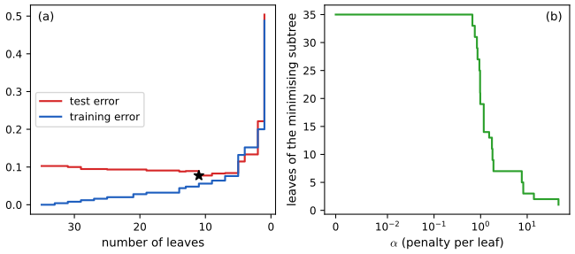
p. 606 Left to grow until every leaf is pure, a tree reaches zero training error (if no two examples share the same inputs with different labels) and overfits. There are two remedies. Early stopping halts growth by a heuristic, such as a minimum number of examples in a node, a maximum depth or a minimum gain (the demonstration has a slider for each). Pruning grows the tree to its maximal size and merges subtrees back into their parents. Pruning can undo a poor greedy choice, which early stopping cannot: the book's example is the XOR data of Figure 13.1, where no single feature has any predictive power, so a learner that stops when the gain is not positive never splits at all.
Filling the gap 18.4: why greedy growing never splits XOR, and cost-complexity pruning p. 606, [BA97b]
Derivation
XOR has zero gain at every first split. Let \(X_1,X_2\) be independent, each symmetric about 0 with no mass at 0, and \(Y=\ind(X_1X_2>0)\). Given \(X_1=x_1\), \(Y=1\) iff \(X_2\) has the same sign as \(x_1\), which has probability \(\frac12\) whatever \(x_1\) is. Hence \(\Pr(Y=1\given X_1)=\frac12\) is constant and, for any threshold \(t\), \(\Pr(Y=1\given X_1\le t)=\Pr(Y=1\given X_1>t)=\frac12\); by symmetry the same holds for a split on \(X_2\). Both children have the parent's class proportions, so by gap 18.3 the gain of any strictly concave impurity is exactly zero. A greedy learner that stops when it cannot improve therefore returns a single leaf with error \(\frac12\), although a tree of depth 2 has error 0. In a finite sample the proportions differ by chance, so tiny positive gains exist and the learner splits on noise; the demonstration shows a best root gain of 1.4% of the cost for 400 noisy XOR points, against 50% for the iris petals. With 25 copies of each of the four corner points every threshold has gain exactly 0 and the tree is one leaf (confirmed numerically).
Cost-complexity pruning. Write \(R(T)=\sum_{\text{leaves }\ell\in T}r(\ell)\) for the training cost of a tree \(T\) (the sum of the weighted impurities of its leaves) and \(|T|\) for its number of leaves. For \(\alpha\ge0\) the penalised cost is \(R_\alpha(T)=R(T)+\alpha|T|\). For a node \(t\) of the full tree \(T_0\) let \(T_t\) be the branch below it. Cutting the branch (making \(t\) a leaf) changes the penalised cost by \(R_\alpha(t)-R_\alpha(T_t)=r(t)-R(T_t)+\alpha(1-|T_t|)\), which is \(\le0\) iff \(\alpha\ge g(t)\) with
\[ g(t)=\frac{r(t)-R(T_t)}{|T_t|-1}\ \ (\ge0\text{ by gap 18.3}). \]
Weakest-link pruning repeatedly cuts the internal node with the smallest \(g(t)\); the successive values \(\alpha_1\le\alpha_2\le\dots\) (made non-decreasing by taking the running maximum) and the nested subtrees \(T_0\supset T_1\supset\dots\supset\{\text{root}\}\) it produces contain, for each \(\alpha\), the smallest subtree minimising \(R_\alpha\): for \(\alpha\) between \(\alpha_k\) and \(\alpha_{k+1}\) the minimiser is \(T_k\) (Breiman et al., 1984, Chapter 3). The proof is an induction on the tree: at a node, the best pruned subtree is either the node as a leaf, or the union of the best subtrees of the two children, and cutting at \(g(t)\le\alpha\) is exactly the comparison between these two. The path is implemented in the code (prune_path) and reproduces scikit-learn's cost-complexity path (the alphas agree to \(10^{-6}\) on an iris tree and on a regression tree). Then \(\alpha\) is chosen by cross-validation or a validation set. Figure 18.S8 shows the path for the two-moons data. \(\square\)
18.1.4 Handling missing input features
p. 606 A discriminative model usually needs every input (Section 1.5.5). Trees have two simple heuristics. Surrogate splits: at each node, besides the best split, record other splits that send the examples the same way as often as possible (the "backup" variables); when the primary variable is missing at test time, use the best available surrogate. This amounts to learning, locally, which other features carry the same information as the chosen one: a local model of the dependence between inputs that does not need the whole joint distribution, at the price of being ad hoc. For a categorical feature the simplest remedy is to add "missing" as one more value and treat the data as fully observed; the learner can then also exploit informative missingness.
18.1.5 Pros and cons
pp. 606–608 Trees are easy to interpret, handle mixed discrete and continuous inputs, are insensitive to monotone transformations of the inputs (no standardisation), select variables automatically, are fast to fit and are relatively robust to outliers. Their main weakness is predictive accuracy, partly because of the greedy fit, and instability: a small change in the data can change the tree a lot because an early split decides everything below it (Figure 18.3). Two of the advantages need a precise statement:
Filling the gap 18.5: invariance to monotone transformations, and what "robust to outliers" means pp. 606–607
Derivation
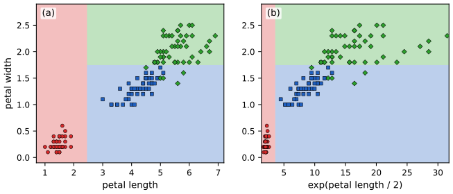
Invariance. Let \(\phi_j\) be a strictly increasing function applied to feature \(j\), \(x'_{nj}=\phi_j(x_{nj})\). The candidate partitions \(\{x_{nj}\le t\}\) of the examples at a node are the sets of the first \(k\) examples in the sorted order of feature \(j\), and the sorted order of \(\phi_j(x_{nj})\) is the same as that of \(x_{nj}\). So the set of candidate partitions is the same for the original and the transformed data, the costs depend on the data only through the partitions, and the greedy algorithm (with the same rule for breaking ties) makes the same choices at every node. The tree built on the transformed data has the same leaves, and a new point \(\bm x\) is sent to the same leaf as \(\bm\phi(\bm x)\) in the transformed tree if the thresholds are mapped by \(\phi_j\) (a midpoint \(t\) between two data values becomes some \(t'\) between their images). So predictions on the training data are identical. Figure 18.S9 shows the iris tree for petal length and for \(\exp(\text{petal length}/2)\): the same partition. (A linear or distance-based model would change.)
Outliers in the inputs. Replace the largest value of a feature by an arbitrarily larger one: the ranks are unchanged, hence so are the partitions (and the training predictions; numerically confirmed). The tree is therefore insensitive to outliers in the inputs.
Outliers in the response. The squared-error leaf value is a mean (18.3) and the split gain is a squared mean difference (gap 18.2). One response \(y_1\to y_1+\Delta\) moves its leaf mean by \(\Delta/|\mathcal D_j|\) and changes the split gain by an amount that grows like \(\Delta\), so it can change the tree structure: a regression tree with squared error is not robust to outliers in the response (numerically, a shift of 100 in one response changes the training predictions by more than 1). A classification tree is robust to a flipped label in the sense that the leaf proportions move by only \(1/|\mathcal D_j|\); leaf values based on the median (absolute loss) or a Huber loss restore robustness in regression (gap 18.16). \(\square\)
Filling the gap 18.6: why a tree is unstable, and how unstable it is p. 608, Figure 18.3
Derivation
Discontinuity of the arg-min. At a node the learner picks \((j,t)\) minimising a score \(s(j,t;\mathcal D)\) over a finite set of candidates. The chosen candidate is a piecewise constant function of the data: if the best and second-best scores differ by \(\epsilon\), changing the data so that each score moves by more than \(\epsilon/2\) reverses the order. Deleting one example of \(n\) at the node moves every score by an amount of order one example, so a node whose best two splits are within one example of each other can change completely. Two kinds of near-ties are common: two different splits with almost the same cost, and, at the leaves, a class tie such as (0, 1, 1) that is resolved by the order of the classes. In the iris tree of Figure 18.3, the leaf holding one versicolor and two virginica flowers (petal width above 1.75, petal length up to 4.85) becomes a tie when one of the two virginica is deleted, and its label flips; the partition changes on 12.8% of the plane although every split is the same.
Propagation. Everything below a changed split is fitted on different subsets, so a change in an early split is amplified through the whole subtree: this is the "hierarchical" instability the book mentions. Instability is a statement about the learning algorithm, a high-variance function of the data; a given fitted tree is perfectly deterministic.
How large is it? The book's claim that one deleted point can change the tree "dramatically" needs qualifying. A single deletion is a mild perturbation, and in my experiments it usually changes nothing: for the depth-3 iris tree 4% of the 150 deletions change the partition at all, by 0.2% of the plane on average (at most 12.8%); for the full tree on 250 two-moons points the mean change is 0.3% of the plane (at most 7.6%). A bootstrap resample, which leaves out about 37% of the points and repeats others, is a much stronger perturbation, and that is what bagging uses: two depth-3 iris trees fitted to independent bootstrap samples disagree on about 17% of the plane (0.16 and 0.18 in two runs of 30 pairs), and two fully grown moons trees on 11% (30 pairs). Averaging cures this: two independent bags of 50 trees disagree on only 1.5% of the moons plane (10 pairs of bags). So the instability that matters is instability under resampling, and averaging (gap 18.9) is the remedy. Figure 18.3d averages the two trees of (b) and (c) and gives a partition between them. \(\square\)
See also: Elements of Statistical Learning, 9.2.2 regression trees and 9.2.4 other issues (pruning, missing data); Introduction to Statistical Learning, 8.1.1 regression trees; Bayesian and Probabilistic ML, 14.4 tree-based models; demos tree pruning, regression tree.
18.2 Ensemble learning
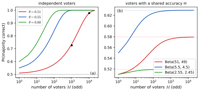
p. 608 Trees have high variance (Section 18.1.5), and the simplest way to reduce the variance of an estimator is to average several of them. An ensemble averages the predictions of \(M\) base models, \[ f(y\given\bm x)=\frac1{|\mathcal M|}\sum_{m\in\mathcal M}f_m(y\given\bm x). \tag{18.10} \] The ensemble has about the same bias as the base models (exactly the same when they are identically distributed) and a lower variance (gap 18.9). For classifiers one can also take a majority vote of the hard decisions (a committee). If each of \(M\) base classifiers is correct with probability \(\theta\) and they err independently, the number of correct votes \(S=\sum_mY_m\) is \(\operatorname{Bin}(M,\theta)\) and the committee is correct with probability \[ p=\Pr(S>M/2)=1-B(M/2,M,\theta), \tag{18.11} \] with \(B\) the binomial cdf. For \(\theta=0.51\) this is 0.726 for \(M=1000\) and 0.977 for \(M=10{,}000\) (the book prints 0.73 and 0.97; 0.977 rounds to 0.98): hundreds or thousands of barely-better-than-chance voters give a good committee, provided they are independent. In practice their mistakes are correlated, and what limits the gain is then not the number of voters but their correlation.
Filling the gap 18.7: the majority-vote probability, its rate, and the ceiling when voters are correlated p. 608, (18.11)
Derivation
The formula. With independent votes \(Y_m\sim\operatorname{Ber}(\theta)\), \(S\sim\operatorname{Bin}(M,\theta)\) and the committee is correct iff \(S>M/2\), so \(p=\Pr(S>M/2)=1-\Pr(S\le M/2)=1-B(\lfloor M/2\rfloor,M,\theta)\) (for even \(M\) a tie \(S=M/2\) is counted as wrong, as in the book's strict inequality). Numerical values: \(M=1000\): 0.7261; \(M=1001\): 0.7366; \(M=10{,}000\): 0.9767. A Monte Carlo estimate with 200,000 draws for \(M=1001\) agrees to three decimals.
Speed. By the central limit theorem \(p\approx\Phi\big(\sqrt M\,(2\theta-1)/(2\sqrt{\theta(1-\theta)})\big)\); for \(\theta=0.51\) the argument is \(0.02\sqrt M/(2\cdot0.49993)\approx0.02\sqrt M\), so \(M=1000\) gives \(\Phi(0.63)=0.74\) and \(M=10^4\) gives \(\Phi(2)=0.977\). Hoeffding's inequality gives the non-asymptotic statement: \(\Pr(S\le M/2)=\Pr(S-M\theta\le-M(\theta-\frac12))\le\exp(-2M(\theta-\frac12)^2)\), so the error of the committee decays exponentially in \(M\), at a rate set by the square of the advantage \(\theta-\frac12\). (For \(\theta=0.51\) the bound is loose: it equals 0.82 at \(M=1000\).) How many voters are needed for 99%? Solving numerically: 539 (odd \(M\)) for \(\theta=0.55\) and 133 for \(\theta=0.60\) (Exercise 18.3).
Correlated voters. The independence assumption is essential. A simple model of dependence is exchangeable: there is a shared random accuracy \(\Theta\) (how "easy" the example is), and given \(\Theta\) the votes are independent \(\operatorname{Ber}(\Theta)\). Then \(\Pr(S>M/2)=\E[\Pr(\operatorname{Bin}(M,\Theta)>M/2\given\Theta)]\). By the law of large numbers \(S/M\to\Theta\) almost surely, so for every \(\Theta\ne\frac12\) the conditional probability tends to \(\ind(\Theta>\frac12)\); since it is bounded by 1, dominated convergence gives \[ \lim_{M\to\infty}\Pr(S>M/2)=\Pr(\Theta>\tfrac12)\ <\ 1\quad\text{unless }\Pr(\Theta>\tfrac12)=1. \] More voters never push the accuracy beyond the probability that the typical voter is better than chance. The correlation between two votes is \(\operatorname{cov}(Y_1,Y_2)=\operatorname{var}\Theta\), i.e. \(\rho=\operatorname{var}\Theta/(\E\Theta(1-\E\Theta))\). For \(\Theta\sim\operatorname{Beta}(5.5,4.5)\) (mean 0.55) the correlation is \(1/(a+b+1)=1/11=0.09\), small, yet the ceiling is \(\Pr(\Theta>\frac12)=0.629\), far below the 99% reached by 539 independent voters of the same average accuracy. Figure 18.S1b shows the curves approaching their ceilings. This is why ensemble methods work hard to make the members diverse: bootstrap samples (bagging), random feature subsets (random forests), and sequential re-weighting (boosting). \(\square\)
18.2.1 Stacking
pp. 608–609 Instead of an unweighted average one can learn how to combine the base models, \(f(y\given\bm x)=\sum_{m\in\mathcal M}w_mf_m(y\given\bm x)\) (18.12), called stacked generalisation (Wolpert, 1992). The weights must be fitted on data that the base models have not seen; otherwise they pile up on the model that fits the training set best.
18.2.2 Ensembling is not Bayes model averaging
p. 609 An ensemble uses the hypothesis class \(p(y\given\bm x,\bm w,\bm\theta)=\sum_mw_mp(y\given\bm x,\bm\theta_m)\) (18.13) with arbitrary weights, whereas Bayes model averaging (BMA, Section 4.6) uses \(p(y\given\bm x,\mathcal D)=\sum_mp(m\given\mathcal D)\,p(y\given\bm x,m,\mathcal D)\) (18.14) with posterior model probabilities that sum to one and, as \(N\to\infty\), concentrate on a single model (Minka, 2000).
Filling the gap 18.8: stacking needs held-out data, and why BMA collapses while an ensemble does not pp. 608–609, (18.12)–(18.14)
Derivation
Why stacking weights need separate data. Suppose base model 1 interpolates the training set (a 1-nearest-neighbour regressor, or a fully grown tree), \(f_1(\bm x_n)=y_n\) for all \(n\). The training least-squares objective \(\sum_n(y_n-\sum_mw_mf_m(\bm x_n))^2\) is then zero at \(\bm w=(1,0,\dots,0)\), the global minimum, so training-set stacking selects exactly the model that has overfit the most (the minimiser is unique when the columns of the matrix of base-model predictions are linearly independent). Numerically, with 60 noisy points from a sine curve, non-negative least squares on the training predictions of a 1-NN regressor and a linear fit gives weights (1.00, 0.00); on 400 held-out points the weights are (0.72, 0.28). The same reasoning applies to any flexible base model, which is why stacking is fitted on out-of-fold or held-out predictions (cross-validated predictions, as in leave-one-out stacking).
BMA concentrates. For two models with posterior \(p(m\given\mathcal D)\propto p(\mathcal D\given m)p(m)\) and i.i.d. data from a true density \(p^*\), the log posterior odds are \(\log\frac{p(\mathcal D\given m_1)}{p(\mathcal D\given m_2)}=\sum_n\log\frac{\bar p_1(\bm x_n)}{\bar p_2(\bm x_n)}+\log\frac{p(m_1)}{p(m_2)}\), with \(\bar p_k\) the marginal-likelihood-averaged predictive. By the law of large numbers this is \(N[\KL(p^*\|\bar p_2)-\KL(p^*\|\bar p_1)]+o(N)\). If the two KL divergences differ, the odds go to \(0\) or \(\infty\) exponentially fast in \(N\) and all posterior mass sits on the model closer to the truth; the weights sum to one at every \(N\), and in the limit one of them is 1. BMA is an average over uncertainty about which single model is right (it assumes one of them is), not a richer model.
An ensemble is not constrained that way. Let the truth be the mixture \(p^*=0.7\,\N(-2,1)+0.3\,\N(2,1)\), with the two base models \(M_1=\N(-2,1)\) and \(M_2=\N(2,1)\). The average log score under the truth is \(-3.82\) for \(M_1\), \(-7.02\) for \(M_2\); so \(\KL(p^*\|M_1)=1.84<\KL(p^*\|M_2)=5.04\) and BMA converges to \(M_1\) with score \(-3.82\) per observation. The ensemble \(\sum_mw_mp_m\) with \(\bm w=(0.7,0.3)\) is the truth and scores \(-1.98\) per observation (the entropy of \(p^*\)). The weights of an ensemble are free parameters fitted to improve prediction, which can mix models none of which is right; those of BMA are posterior probabilities of a hypothesis. For regression ensembles the weights need not even sum to one. (Numbers computed by quadrature.) \(\square\)
See also: Elements of Statistical Learning, 8.8 model averaging and stacking; Bayesian and Probabilistic ML, 14.1 Bayesian model averaging and 14.2 committees.
18.3 Bagging
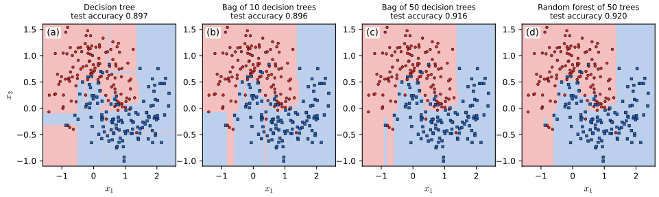
pp. 609–610 Bagging ("bootstrap aggregating"; Breiman, 1996) fits \(M\) base models, each to a bootstrap sample of the training set: \(N\) examples drawn with replacement from the \(N\) originals (Section 4.7.3). The predictions are averaged (or voted). A given bootstrap sample contains each original example with probability \(1-(1-1/N)^N\to1-e^{-1}\approx0.63\), so a base model sees only about 63% of the distinct examples. The other 37% are out of bag (OOB) for that model, and the model's performance on them estimates test performance, an alternative to cross-validation. The benefit is that no individual example dominates the ensemble, which gives robustness (Grandvalet, 2004); the more trees, the better, at the price of memory and time (Figure 18.4). Bagging helps only if the base learner is unstable, so that omitting data changes the fit: trees are, nearest-neighbour classifiers are not, and deep networks, which need all the data, usually do not benefit (Nakkiran et al., 2020).
Filling the gap 18.9: the 63% rule, the variance of an average of correlated trees, Jensen's inequality for aggregation, and the out-of-bag estimate pp. 609–610
Derivation
The 63% rule. A given example is missed by one draw with probability \(1-1/N\), so by all \(N\) independent draws with probability \((1-1/N)^N\). Taking logarithms, \(N\log(1-1/N)=-\sum_{k\ge1}\frac1{kN^{k-1}}=-1-\frac1{2N}-\frac1{3N^2}-\dots\), which increases with \(N\) towards \(-1\). Hence \((1-1/N)^N\) increases to \(e^{-1}=0.3679\) from below and the expected fraction of distinct examples in a bootstrap sample, \(1-(1-1/N)^N\), decreases to \(0.632\) from above: 0.6415 for \(N=20\) (12.83 distinct examples), 0.6323 for \(N=1000\) (a simulation agrees to within 0.004). The probability that a given example is OOB for a given tree is \((1-1/N)^N\), so it is OOB for about \(0.368B\) of \(B\) trees (observed: 0.365).
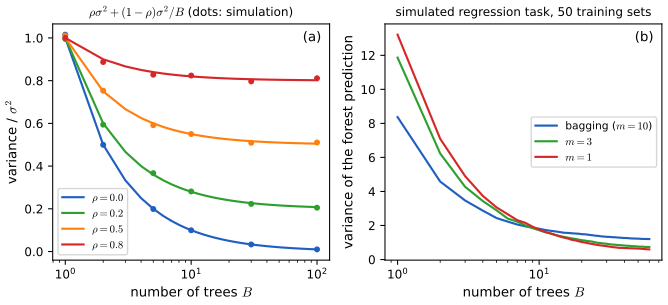
Variance of an average. Let \(T_1,\dots,T_B\) be identically distributed with variance \(\sigma^2\) and pairwise correlation \(\rho\) (the correlation arises because all trees see the same data). Then \[ \operatorname{var}\Big(\frac1B\sum_bT_b\Big)=\frac1{B^2}\Big[\sum_b\operatorname{var}T_b+\sum_{b\ne b'}\operatorname{cov}(T_b,T_{b'})\Big]=\frac{\sigma^2}B+\frac{B(B-1)}{B^2}\rho\sigma^2=\rho\sigma^2+\frac{1-\rho}B\sigma^2. \] The mean of the average equals the common mean of the \(T_b\), so the bias is unchanged. As \(B\to\infty\) the variance tends to \(\rho\sigma^2\): a floor set by the correlation, not by \(B\) (Figure 18.S2a; for \(\rho=0.3\), \(B=25\) the simulated variance is 0.328 against \(0.3+0.7/25=0.328\)). Bootstrap trees fitted to one data set are identically distributed but not independent, hence \(\rho>0\); making \(\rho\) smaller is the aim of random forests (gap 18.10).
Aggregation never hurts (Breiman, 1996). Let \(\varphi(\bm x,L)\) be a predictor trained on a random training set \(L\) and \(\varphi_A(\bm x)=\E_L\varphi(\bm x,L)\) the aggregated predictor. For squared error and any fixed \(y\), Jensen's inequality for the convex function \(u\mapsto(y-u)^2\) gives \((y-\varphi_A(\bm x))^2\le\E_L(y-\varphi(\bm x,L))^2\); averaging over \((\bm x,y)\) gives \(\E(y-\varphi_A)^2\le\E(y-\varphi)^2\). The gap is exactly the variance of the predictor: \(\E_L(y-\varphi)^2-(y-\varphi_A)^2=\operatorname{var}_L\varphi(\bm x,L)\). The more unstable the predictor (the larger its variance over training sets), the more aggregation gains; a stable predictor has nothing to gain. In an experiment with 100 independent training sets of 60 points from \(y=\sin3x+\)noise, the mean squared error of single regression trees (leaves of at least 2 points) against the true curve was 0.060 and that of their average 0.001. Bagging approximates the aggregate by averaging over bootstrap resamples of one training set, so it can reduce only the variance that comes from the resampling variability, and the bootstrap trees are a little worse than trees on fresh samples (they see about 63% of the distinct points). For classifiers aggregation is subtler: a majority vote at \(\bm x\) moves the correct-class probability to 1 if the base classifier is correct there with probability above \(\frac12\) and to 0 if below (gap 18.7 with \(M\to\infty\)), so voting improves a good classifier and worsens a bad one.
Out-of-bag estimate. The \(b\)-th tree is trained without the OOB examples, so its prediction at an OOB example \(\bm x_i\) is an honest out-of-sample prediction. For example \(i\), the average of the \(\approx0.37B\) trees for which it is OOB gives an out-of-sample ensemble prediction, and the average loss over \(i\) is the OOB error. As \(B\to\infty\) it converges to the leave-one-out bootstrap error (the expected loss at \(\bm x_i\) of a tree fitted to a bootstrap sample that excludes \(i\)). It estimates the error of a smaller bag (about 37% as many trees, trained on 63% as many distinct points), so it is slightly pessimistic for the full bag. Over 8 simulated two-moons data sets of 250 points the mean OOB error of a 100-tree bag was 0.102, the mean test error of the full bag 0.093 and that of a bag of the first 37 trees 0.095, i.e. the OOB error tracks the error of the 37-tree bag. A single data set can differ by more: one 100-tree bag had OOB error 0.132 against test error 0.085 (the standard error of an error rate of 0.1 estimated from 250 points is about 0.02). \(\square\)
See also: Elements of Statistical Learning, 8.7 bagging and 15.3.1 out-of-bag samples; Introduction to Statistical Learning, 8.2.1 bagging; demos bagging trees, out-of-bag error, bootstrap inclusion.
18.4 Random forests
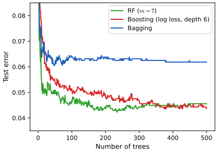
pp. 610–611 Bagging assumes that re-running the same algorithm on different subsets of the data gives sufficiently different models. Random forests (Breiman, 2001) decorrelate the trees further: besides bootstrapping the examples, each split is searched over only a random subset \(S_i\subset\{1,\dots,D\}\) of the features, i.e. \(j\) in (18.5) ranges over \(S_i\). The spam e-mail data (4601 messages, 57 inputs: 48 word percentages, 6 character percentages and 3 capital-letter statistics; Hastie et al., 2009) illustrate the effect in Figure 18.5: a forest beats bagged trees clearly and boosting (Section 18.5) beats both, but boosting must fit its trees one after another, whereas the trees of a forest can be fitted in parallel.
Filling the gap 18.10: why random feature subsets help, the correlation of two trees and the role of the subset size pp. 610–611
Derivation
Correlation of two trees of a forest. Let \(Z\) be the training data (random) and \(\Theta\) the randomisation of one tree (bootstrap sample and feature subsets), with \(\Theta_1,\Theta_2\) independent given \(Z\). Write \(T_b=T(\bm x;\Theta_b,Z)\). Both have the same marginal law, with variance \(\sigma^2(\bm x)\) over \((Z,\Theta)\). By conditioning on \(Z\), \(\operatorname{cov}(T_1,T_2)=\E[\operatorname{cov}(T_1,T_2\given Z)]+\operatorname{cov}(\E[T_1\given Z],\E[T_2\given Z])=0+\operatorname{var}_Z(\E[T\given Z])\), since given \(Z\) the two trees are independent. The law of total variance gives \(\sigma^2=\operatorname{var}_Z(\E[T\given Z])+\E_Z\operatorname{var}(T\given Z)\). Hence \[ \rho(\bm x)=\frac{\operatorname{var}_Z(\E_\Theta[T\given Z])}{\operatorname{var}_Z(\E_\Theta[T\given Z])+\E_Z\operatorname{var}_\Theta(T\given Z)}, \] the share of the total variance of a single tree that is due to the data rather than to the internal randomisation; the variance of the forest with \(B\) trees is \(\rho\sigma^2+(1-\rho)\sigma^2/B\) (gap 18.9), and as \(B\to\infty\) it tends to \(\operatorname{var}_Z(\E_\Theta[T\given Z])=\rho\sigma^2\).
What the subset size does. Taking \(m<D\) candidate features per split increases the randomisation of each tree, so \(\E_Z\operatorname{var}_\Theta(T\given Z)\) grows and \(\rho\) falls, which lowers the floor \(\rho\sigma^2\). The price is that each tree is a poorer, noisier fit (a split restricted to a few random features cannot use the best feature when it is not in the subset): \(\sigma^2\) itself and the bias grow as \(m\) shrinks. With \(m=D\) there is no feature randomisation and one has bagging. A good \(m\) balances the two; common defaults are \(\sqrt D\) for classification and \(D/3\) for regression. Figure 18.S2b measures this on Friedman's first benchmark (10 features, 5 relevant, 200 training points, 50 independent training sets, trees with at least 3 points per leaf, predictions at 30 fixed points): the variance of a single tree is 8.4 for bagging (\(m=10\)), 11.9 for \(m=3\) and 13.2 for \(m=1\), but after 60 trees it is 1.20, 0.74 and 0.60: the more random the splits, the lower the floor. The variance is only half the story: the bias of forests with small \(m\) is larger, which is why \(m=1\) is rarely best in practice. \(\square\)
See also: Elements of Statistical Learning, 15.2 definition of random forests, 15.4.1 variance and the de-correlation effect; Introduction to Statistical Learning, 8.2.2 random forests; demos random forest decorrelation, forest decorrelation.
18.5 Boosting
pp. 611–612 Bagged trees and forests are additive models \[ f(\bm x;\bm\theta)=\sum_{m=1}^M\beta_mF_m(\bm x;\bm\theta_m),\qquad\beta_m=1/M\text{ for an average}, \tag{18.15} \] and one can allow the \(F_m\) to be any function approximator, not only trees: a linear model with adaptive basis functions (Hastie et al., 2009). The goal is to minimise the empirical loss \(L(f)=\sum_{i=1}^N\ell(y_i,f(\bm x_i))\) (18.16), possibly plus a regulariser. Boosting (Schapire, 1990; Freund and Schapire, 1996) fits the additive model sequentially: \(F_1\) on the data, then \(F_2\) on the data re-weighted to emphasise what \(F_1\) got wrong, and so on for \(M\) rounds. \(M\) is a complexity parameter, chosen by early stopping on a validation set. Where bagging and forests fit identically distributed (and correlated) trees and reduce variance, boosting fits trees that depend on each other and mainly reduces bias. The book states that if each \(F_m\) beats chance, even on the re-weighted data, the ensemble is better than its members; gap 18.12 proves the exact statement for AdaBoost. The rest of the section follows the statistical view of Friedman, Hastie and Tibshirani (2000) and Friedman (2001), which allows any differentiable loss (regression, multiclass classification, ranking).
Filling the gap 18.12: weak learners become strong, the training-error bound of AdaBoost p. 612, [SF12]
Proof
Setting. Run discrete AdaBoost (Algorithm 18.1, derived in gap 18.13) on \(\tilde y_i\in\{-1,+1\}\). Let \(\omega_i^{(m)}\) be the weights in round \(m\), normalised to sum to 1, \(F_m\in\{-1,+1\}\) the learner fitted with them, \(\epsilon_m=\sum_i\omega_i^{(m)}\ind(\tilde y_i\ne F_m(\bm x_i))\) its weighted error, \(\alpha_m=\log\frac{1-\epsilon_m}{\epsilon_m}\) and \(f_M(\bm x)=\sum_{m\le M}\alpha_mF_m(\bm x)\), so that the classifier is \(\sgn f_M\). Weak-learning assumption: \(\epsilon_m\le\frac12-\gamma_m\) with \(\gamma_m>0\) in every round (the learner beats a coin on whatever weights it is given).
Claim. The training error of \(\sgn f_M\) is at most \(\prod_{m=1}^M2\sqrt{\epsilon_m(1-\epsilon_m)}=\prod_m\sqrt{1-4\gamma_m'^2}\le\exp(-2\sum_m\gamma_m'^2)\), where \(\gamma_m'=\frac12-\epsilon_m\ge\gamma_m\). In particular, if \(\gamma_m\ge\gamma>0\) always, the training error is at most \(e^{-2\gamma^2M}\) and is zero once \(M>\ln N/(2\gamma^2)\).
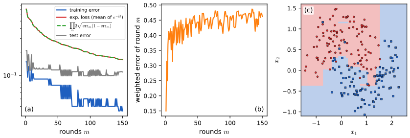
Proof. (1) The 0-1 loss is below the exponential loss. If \(\sgn f_M(\bm x_i)\ne\tilde y_i\) then \(\tilde y_if_M(\bm x_i)\le0\) and \(e^{-\tilde y_if_M(\bm x_i)/2}\ge1\); so \(\frac1N\sum_i\ind(\sgn f_M(\bm x_i)\ne\tilde y_i)\le\frac1N\sum_ie^{-\tilde y_if_M(\bm x_i)/2}\) (the factor \(\frac12\) is the book's: its \(f=\frac12\sum_m\alpha_mF_m\), see (18.34)–(18.35)). (2) The exponential loss is a product. Let \(W_m=\sum_i e^{-\tilde y_if_{m}(\bm x_i)/2}\), \(W_0=N\). Then \[ W_m=\sum_ie^{-\tilde y_if_{m-1}(\bm x_i)/2}e^{-\alpha_m\tilde y_iF_m(\bm x_i)/2}=W_{m-1}\sum_i\omega_i^{(m)}e^{-\alpha_m\tilde y_iF_m(\bm x_i)/2}, \] because \(\omega_i^{(m)}=e^{-\tilde y_if_{m-1}(\bm x_i)/2}/W_{m-1}\) (the update (18.33) with normalisation). The last sum is \((1-\epsilon_m)e^{-\alpha_m/2}+\epsilon_me^{\alpha_m/2}\) (correct examples have \(\tilde yF=1\), wrong ones \(-1\)); with \(e^{\alpha_m/2}=\sqrt{(1-\epsilon_m)/\epsilon_m}\) this equals \((1-\epsilon_m)\sqrt{\epsilon_m/(1-\epsilon_m)}+\epsilon_m\sqrt{(1-\epsilon_m)/\epsilon_m}=2\sqrt{\epsilon_m(1-\epsilon_m)}=:Z_m\). So \(W_M=N\prod_mZ_m\) and the mean exponential loss after \(M\) rounds is exactly \(\prod_mZ_m\) (confirmed numerically on the two-moons data: equal to \(10^{-10}\) relative accuracy). (3) The numerical bound. With \(\epsilon=\frac12-\gamma'\), \(Z=2\sqrt{(\frac12-\gamma')(\frac12+\gamma')}=\sqrt{1-4\gamma'^2}\), and \(1-u\le e^{-u}\) gives \(Z\le e^{-2\gamma'^2}\). (4) Zero error. The training error is a multiple of \(1/N\) and is \(\le e^{-2\gamma^2M}<1/N\) once \(M>\ln N/(2\gamma^2)\), so it is exactly 0. \(\square\)
Remarks. The theorem says nothing about the test error (the ensemble can drive the training error to 0 and still generalise, which is explained by margins; Schapire et al., 1998), and it fails if the weak-learning assumption fails: on data with contradictory labels a learner cannot stay better than chance on all re-weightings. Because the weights move to the hardest points, the weighted error of the learners drifts up towards \(\frac12\) as rounds go by (Figure 18.S3b), so the bound's exponent grows more slowly with \(m\) than at the start.
18.5.1 Forward stagewise additive modeling
p. 612 In forward stagewise additive modelling the model is grown one term at a time without revisiting earlier terms: at round \(m\), \[ (\beta_m,\bm\theta_m)=\argmin_{\beta,\bm\theta}\sum_{i=1}^N\ell\big(y_i,f_{m-1}(\bm x_i)+\beta F(\bm x_i;\bm\theta)\big),\qquad f_m(\bm x)=f_{m-1}(\bm x)+\beta_mF(\bm x;\bm\theta_m). \tag{18.17, 18.18} \] How to solve the inner problem depends on the loss and on the weak learner.
18.5.2 Quadratic loss and least squares boosting
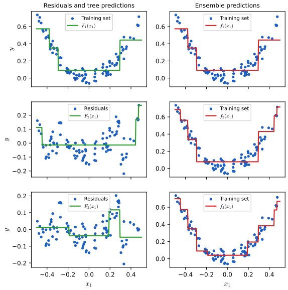
pp. 612–613 For \(\ell(y,\hat y)=(y-\hat y)^2\) the \(i\)-th term of the round-\(m\) objective is \((y_i-f_{m-1}(\bm x_i)-\beta F(\bm x_i))^2=(r_{im}-\beta F(\bm x_i))^2\) with the residual \(r_{im}=y_i-f_{m-1}(\bm x_i)\) (18.19), so one sets \(\beta=1\) and fits \(F\) to the residuals: least squares boosting (Bühlmann and Yu, 2003). Figure 18.6 shows three rounds with depth-2 regression trees on a one-dimensional problem; each new tree corrects the errors of the previous ensemble. The gradient-boosting demonstration lets you vary the number of rounds, the depth and the loss.
Filling the gap 18.11: why forward stagewise, and why \(\beta=1\) for squared loss pp. 612–613, (18.17)–(18.19)
Derivation
Why not optimise everything at once? The joint problem \(\min_{\{\beta_m,\bm\theta_m\}}\sum_i\ell(y_i,\sum_m\beta_mF(\bm x_i;\bm\theta_m))\) is non-convex in the tree structures and has \(O(M)\) times as many parameters. The stagewise rule keeps the cost of each round equal to that of fitting one tree and never changes the earlier trees, which makes the sequence cheap and a natural form of regularisation: later terms can only explain what the earlier ones missed. (Joint optimisation, "backfitting", can fit the training data better but is slower and overfits more easily; Hastie et al., 2009, Section 10.2.)
Squared loss. For fixed \(\bm\theta\), put \(\bm u=(F(\bm x_i;\bm\theta))_i\) and \(\bm r=(r_{im})_i\). The objective \(\|\bm r-\beta\bm u\|^2\) is minimised over \(\beta\) at \(\beta=\bm r^\T\bm u/\bm u^\T\bm u\), the regression coefficient of the residuals on the learner. (i) If the weak-learner class is closed under multiplication by a constant (a regression tree with free leaf values is: multiply all leaf values), \(\beta F\) is again in the class, so \(\beta\) can be absorbed into \(F\) and the stage solves \(\min_F\sum_i(r_{im}-F(\bm x_i))^2\): "set \(\beta=1\) and fit \(F\) to the residuals". (ii) If the learner outputs \(\pm1\) (a classifier) the optimal \(\beta\) is \(\sum_ir_{im}F_i/N\). In both cases the new residuals are \(\bm r-\beta\bm u\), so each stage is a least-squares regression of the current residuals; the training loss never increases because \(\beta=0\) is feasible. With shrinkage, \(f_m=f_{m-1}+\nu F_m\) with \(0<\nu\le1\), the residuals shrink by the factor \((1-\nu)\) along the directions the learner can fit, so many more rounds are needed but the fit follows a smoother path, a form of regularisation; for componentwise linear learners and \(\nu\to0\) the path approaches the lasso (Efron et al., 2004). Numerically, the least-squares-boosting loop \(f\leftarrow f+\nu F\) with \(F\) fitted to \(y-f\) coincides with the general gradient-boosting code for squared loss (identical to \(10^{-12}\)) and with scikit-learn's squared-error boosting (to \(10^{-16}\)), and its training loss is non-increasing. \(\square\)
18.5.3 Exponential loss and AdaBoost
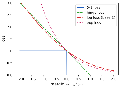
pp. 613–615 For binary classification with \(\tilde y_i\in\{-1,+1\}\) let the learner output \(F(\bm x)\), half the log-odds, so that \(p(y=1\given\bm x)=e^{F}/(e^{-F}+e^{F})=1/(1+e^{-2F(\bm x)})\) (18.20). The negative log-likelihood is \(\ell(\tilde y,F)=\log(1+e^{-2\tilde yF(\bm x)})\) (18.21) (Equation 10.13), a smooth convex upper bound on the 0-1 loss as a function of the margin \(m=\tilde yF(\bm x)\) (Figure 18.7). One may also use the exponential loss \(\ell(\tilde y,F)=\exp(-\tilde yF(\bm x))\) (18.22), also a smooth upper bound. Its population minimiser is the same as for the log loss (18.23)–(18.25), but it is easier to optimise in the boosting setting. Fitting the stage-\(m\) problem with a learner that returns a label \(F_m\in\{-1,+1\}\) gives discrete AdaBoost (Freund and Schapire, 1996; Friedman et al., 2000).
Filling the gap 18.13: the population minimiser, the stage solution of AdaBoost, the weight update, and two identities pp. 614–616, (18.23)–(18.35), Algorithm 18.1
Derivation
The population minimiser (18.23)–(18.25). Fix \(\bm x\) and let \(p=\Pr(\tilde y=1\given\bm x)\). The conditional expected exponential loss is \(\phi(F)=pe^{-F}+(1-p)e^{F}\), strictly convex in \(F\) with \(\phi'(F)=-pe^{-F}+(1-p)e^{F}\), which vanishes at \(e^{2F}=p/(1-p)\): \(F^*=\frac12\log\frac p{1-p}\), half the log-odds, so the posterior probability can be recovered as \(p=1/(1+e^{-2F^*})\) at the population level. For the loss (18.21), \(\frac{\d}{\d F}\log(1+e^{-2\tilde yF})=-2\tilde y\sigma(-2\tilde yF)\), so the conditional expected derivative is \(-2p\sigma(-2F)+2(1-p)\sigma(2F)=-2p(1-\sigma(2F))+2(1-p)\sigma(2F)=2(\sigma(2F)-p)\), zero iff \(\sigma(2F)=p\): the same minimiser. (Numerically both agree for \(p\in\{0.1,0.3,0.7,0.9\}\).) The two losses differ only in how they punish a given margin, and in the tails (below). The three upper-bound statements of Figure 18.7: for \(m\le0\), \(e^{-m}\ge1\), \(\log_2(1+e^{-m})\ge\log_22=1\), \(\max(0,1-m)\ge1\); for \(m>0\) all are \(\ge0=\)the 0-1 loss.
The stage problem (18.26)–(18.29). With \(\omega_{i,m}=e^{-\tilde y_if_{m-1}(\bm x_i)}\), \(L_m=\sum_i\omega_{i,m}e^{-\beta\tilde y_iF(\bm x_i)}\). For \(F(\bm x_i)\in\{-1,+1\}\), \(\tilde y_iF(\bm x_i)=1\) if correct and \(-1\) if wrong, so \(L_m=e^{-\beta}A+e^{\beta}B\) with \(A=\sum_{\text{correct}}\omega_{i,m}\), \(B=\sum_{\text{wrong}}\omega_{i,m}\). Writing \(A=\sum_i\omega_{i,m}-B\), \(L_m=(e^{\beta}-e^{-\beta})B+e^{-\beta}\sum_i\omega_{i,m}\), (18.28). For any \(\beta>0\) the factor \(e^\beta-e^{-\beta}\) is positive, so minimising over \(F\) means minimising the weighted number of mistakes \(B=\sum_i\omega_{i,m}\ind(\tilde y_i\ne F(\bm x_i))\): fit the weak learner to the data with weights \(\omega_{i,m}\) (18.29). Then minimise over \(\beta\): \(\partial_\beta L_m=-e^{-\beta}A+e^{\beta}B=0\) gives \(e^{2\beta}=A/B\), \(\beta_m=\frac12\log\frac{A}{B}=\frac12\log\frac{1-\epsilon_m}{\epsilon_m}\) with \(\epsilon_m=B/(A+B)\) the weighted error (18.30)–(18.31); the second derivative \(e^{-\beta}A+e^\beta B>0\) makes it the minimum. This needs \(\epsilon_m<\frac12\) for \(\beta_m>0\); if the best learner has \(\epsilon_m>\frac12\) its negation has error \(1-\epsilon_m<\frac12\) (a numerical minimisation of \(L_m\) over \(\beta\) for random weights agrees with the formula to \(10^{-5}\)).
The weight update (18.33)–(18.35). \(\omega_{i,m+1}=e^{-\tilde y_if_m(\bm x_i)}=\omega_{i,m}e^{-\beta_m\tilde y_iF_m(\bm x_i)}\). Since \(\tilde y_iF_m(\bm x_i)=1-2\ind(\tilde y_i\ne F_m(\bm x_i))\), \(-\tilde y_iF_m=2\ind(\cdot)-1\), so \(\omega_{i,m+1}=\omega_{i,m}e^{2\beta_m\ind(\tilde y_i\ne F_m(\bm x_i))}e^{-\beta_m}\). The factor \(e^{-\beta_m}\) is the same for all examples and cancels when the weights are normalised, so with \(\alpha_m=2\beta_m=\log\frac{1-\epsilon_m}{\epsilon_m}\) one multiplies the weights of the misclassified examples by \(e^{\alpha_m}\) and leaves the others alone: Algorithm 18.1 (Adaboost.M1). Since \(f_M=\sum_m\beta_mF_m=\frac12\sum_m\alpha_mF_m\) has the same sign as \(\sum_m\alpha_mF_m\), the output is \(\sgn[\sum_m\alpha_mF_m(\bm x)]\). The multiclass version, SAMME, adds \(\log(C-1)\) to \(\alpha_m\) (Zhu et al., 2009); for \(C=2\) the two coincide, and the code agrees with the scikit-learn implementation on all 1000 test points after 20 rounds.
Two identities. (i) After the update, the weighted error of the learner just added is exactly \(\frac12\): the new weights are \(\omega e^{\beta}\) on mistakes and \(\omega e^{-\beta}\) on correct examples, so the new weighted error is \(\epsilon e^{\beta}/(\epsilon e^\beta+(1-\epsilon)e^{-\beta})=\sqrt{\epsilon(1-\epsilon)}/(2\sqrt{\epsilon(1-\epsilon)})=\frac12\), as \(e^\beta=\sqrt{(1-\epsilon)/\epsilon}\). Thus \(F_m\) is no better than a coin on the data \(F_{m+1}\) sees, which is why boosting does not choose the same learner twice in a row. (ii) The mean exponential loss after \(m\) rounds is exactly \(\prod_{k\le m}2\sqrt{\epsilon_k(1-\epsilon_k)}\) (proof in gap 18.12). Both identities are confirmed numerically (exact to \(10^{-10}\)). \(\square\)
Algorithm 18.1: AdaBoost.M1, for binary classification with exponential loss
Input: data \((\bm x_i,\tilde y_i)\), \(\tilde y_i\in\{-1,+1\}\), number of rounds \(M\), a learner that accepts weights.
- \(\omega_i\gets1/N\).
- For \(m=1,\dots,M\): (a) fit \(F_m\) to the weighted training set; (b) \(\operatorname{err}_m\gets\sum_i\omega_i\ind(\tilde y_i\ne F_m(\bm x_i))/\sum_i\omega_i\); (c) \(\alpha_m\gets\log[(1-\operatorname{err}_m)/\operatorname{err}_m]\); (d) \(\omega_i\gets\omega_i\exp[\alpha_m\ind(\tilde y_i\ne F_m(\bm x_i))]\).
- Return \(f(\bm x)=\sgn[\sum_{m=1}^M\alpha_mF_m(\bm x)]\).
See also: Elements of Statistical Learning, 10.4 exponential loss and AdaBoost and 10.5 why exponential loss; Bayesian and Probabilistic ML, 14.3.1 minimising exponential error; demo AdaBoost.
18.5.4 LogitBoost
p. 616 The exponential loss puts a huge weight on misclassified examples (Figure 18.7, left), which makes AdaBoost sensitive to outliers and mislabelled data; and \(e^{-\tilde yf}\) is not the log of any probability mass function on \(\{-1,+1\}\), so the fitted \(f\) is not a calibrated log-odds. The log loss, which grows only linearly for large negative margins, does give probabilities \(p(y=1\given\bm x)=1/(1+e^{-2f(\bm x)})\) (18.36). Minimising \(L(f)=\sum_i\log[1+\exp(-2\tilde y_if(\bm x_i))]\) (18.37) by a Newton step at each stage gives LogitBoost (Friedman et al., 2000), Algorithm 18.2, whose key subroutine is a weighted least-squares fit.
Algorithm 18.2: LogitBoost, for binary classification with log loss
Input: data \((\bm x_i,y_i^*)\) with \(y_i^*\in\{0,1\}\); a learner that fits weighted least squares.
- \(f\gets0\), \(\pi_i\gets1/2\).
- For \(m=1,\dots,M\): (a) working response \(z_i\gets(y^*_i-\pi_i)/(\pi_i(1-\pi_i))\); (b) weights \(\omega_i\gets\pi_i(1-\pi_i)\); (c) \(F_m\gets\argmin_F\sum_i\omega_i(z_i-F(\bm x_i))^2\); (d) \(f(\bm x)\gets f(\bm x)+\frac12F_m(\bm x)\); (e) \(\pi_i\gets1/(1+\exp(-2f(\bm x_i)))\).
- Return \(f(\bm x)=\sgn[\sum_mF_m(\bm x)]\).
Filling the gap 18.14: LogitBoost is Newton's method, and the sensitivity of the exponential loss pp. 616–617, (18.36), (18.37), Algorithm 18.2
Derivation
Derivatives. Write the loss of example \(i\) as \(\ell_i(f_i)=\log(1+e^{-2\tilde y_if_i})\) and \(\pi_i=\sigma(2f_i)\), \(y_i^*=(\tilde y_i+1)/2\in\{0,1\}\). Then \(\ell_i'(f_i)=-2\tilde y_i\sigma(-2\tilde y_if_i)=-2(y_i^*-\pi_i)\) (for \(\tilde y_i=1\) it is \(-2(1-\pi_i)\), for \(\tilde y_i=-1\) it is \(2\pi_i\)), and \(\ell_i''(f_i)=4\pi_i(1-\pi_i)\), using \(\sigma'=\sigma(1-\sigma)\) and \(\frac{\d}{\d f}\pi=2\pi(1-\pi)\). (Numerical differentiation agrees.)
Newton step. If the update could be any number \(\delta_i\) at each training point, Newton's method would set \(\delta_i=-\ell_i'/\ell_i''=\frac{y^*_i-\pi_i}{2\pi_i(1-\pi_i)}=\frac12z_i\), with \(z_i\) the working response of line (a). The learner is restricted to a class \(\mathcal F\), so one minimises the second-order Taylor expansion of the loss over \(F\in\mathcal F\): \(\sum_i[\ell_i'F_i+\frac12\ell_i''F_i^2]=\frac12\sum_i\ell_i''(F_i+\ell_i'/\ell_i'')^2-\mathrm{const}=2\sum_i\pi_i(1-\pi_i)(F_i-\tfrac12z_i)^2-\mathrm{const}\). This is a weighted least-squares problem with weights \(\omega_i=\pi_i(1-\pi_i)\) and target \(\frac12z_i\); the algorithm fits \(F_m\) to the target \(z_i\) with the same weights and adds \(\frac12F_m\), which is the same thing (the minimiser for target \(z\) is twice that for target \(z/2\), for a class closed under scaling). So LogitBoost is "Newton boosting for the log loss" and each round has the form of one IRLS step of logistic regression (Section 10.2.6), with the tree in the role of the linear model. In practice the working response is clipped (to \([-4,4]\) in the code) and the weights floored, since \(z_i\) blows up when \(\pi_i\) is close to 0 or 1. The training log loss falls with the rounds: on the two-moons data with stumps, \(\frac1N\sum_i\log(1+e^{-2\tilde y_if(\bm x_i)})\) is 0.429, 0.263, 0.148 after 1, 5, 30 rounds.
Why log loss is more robust than exponential loss. The influence of an example is the size of the gradient of its loss at its margin \(m_i=\tilde y_if(\bm x_i)\). For the exponential loss it is \(e^{-m_i}\), unbounded as the margin goes to \(-\infty\): an example that is wrong by margin \(-5\) receives 150 times the weight of an example at margin 0, and a mislabelled point keeps gaining weight in every round (the AdaBoost weights multiply by \(e^{\alpha_m}\) at each mistake). For the log loss it is \(2\sigma(-2m_i)\le2\), bounded: mislabelled points have a bounded pull. In the demonstration flipping 10% of the training labels raises the test error of AdaBoost with 150 stumps from 0.111 to about 0.13. The log loss is still unbounded (the book's Section 10.4 treats bounded losses for the extreme case). \(\square\)
18.5.5 Gradient boosting
pp. 616–618 Rather than deriving a new algorithm for each loss, gradient boosting (Friedman, 2001; Mason et al., 2000) does gradient descent on \(L(\bm f)\) in function space, representing the function by its values \(\bm f=(f(\bm x_1),\dots,f(\bm x_N))\) on the training set. At step \(m\) the gradient at \(\bm f_{m-1}\) is \(g_{im}=\partial\ell(y_i,f(\bm x_i))/\partial f(\bm x_i)\) (18.38) (Table 18.1) and the update is \(\bm f_m=\bm f_{m-1}-\beta_m\bm g_m\) (18.39) with the step chosen by line search \(\beta_m=\argmin_\beta L(\bm f_{m-1}-\beta\bm g_m)\) (18.40). This only changes \(\bm f\) at the training points; to generalise, a weak learner is fitted to the negative gradient, \(F_m=\argmin_F\sum_i(-g_{im}-F(\bm x_i))^2\) (18.41), and added with a learning rate \(0<\nu\le1\) (Algorithm 18.3). For squared loss \(-g_{im}=y_i-f_{m-1}(\bm x_i)\) is the residual and one recovers least-squares boosting. For the log loss one obtains BinomialBoost (Bühlmann and Hothorn, 2007), which needs only a black-box regression model, not a weighted fit; for \(C\) classes, \(C\) regression trees are fitted to the pseudo-residuals \(-g_{icm}=\ind(y_i=c)-\pi_{ic}\) (18.42) and combined by a softmax (18.43). Stochastic gradient boosting (Friedman, 1999) fits each tree to a random subsample drawn without replacement, which is faster and regularises.
| Name | Loss \(\ell(y_i,f(\bm x_i))\) | \(-\partial\ell/\partial f(\bm x_i)\) (corrected) | Book's Table 18.1 |
|---|---|---|---|
| Squared error | \(\frac12(y_i-f(\bm x_i))^2\) | \(y_i-f(\bm x_i)\) | same |
| Absolute error | \(|y_i-f(\bm x_i)|\) | \(\sgn(y_i-f(\bm x_i))\) | same |
| Exponential loss | \(\exp(-\tilde y_if(\bm x_i))\) | \(+\tilde y_i\exp(-\tilde y_if(\bm x_i))\) | printed with a minus sign |
| Binary log loss | \(\log(1+e^{-2\tilde y_if_i})\), \(\pi_i=\sigma(2f_i)\) | \(2(y_i-\pi_i)\), \(y_i\in\{0,1\}\) | \(y_i-\pi_i\) for the loss \(\log(1+e^{-\tilde y_if_i})\) (which gives \(y_i-\sigma(f_i)\)) |
| Multiclass log loss | \(-\sum_cy_{ic}\log\pi_{ic}\) | \(y_{ic}-\pi_{ic}\) | same |
Table 18.1 (corrected): common losses and their negative gradients; for the classification rows \(\tilde y_i\in\{-1,+1\}\) and \(y_i=(\tilde y_i+1)/2\). The derivations are in gap 18.15.
Algorithm 18.3: gradient boosting
- Initialise \(f_0(\bm x)=\argmin_F\sum_i\ell(y_i,F(\bm x_i))\) (a constant).
- For \(m=1,\dots,M\): (a) pseudo-residuals \(r_{im}=-[\partial\ell(y_i,f(\bm x_i))/\partial f(\bm x_i)]_{f=f_{m-1}}\); (b) fit a weak learner \(F_m=\argmin_F\sum_i(r_{im}-F(\bm x_i))^2\); (c) \(f_m(\bm x)=f_{m-1}(\bm x)+\nu F_m(\bm x)\).
- Return \(f(\bm x)=f_M(\bm x)\).
Filling the gap 18.15: gradient boosting as functional gradient descent, the entries of Table 18.1 and the descent guarantee pp. 616–618, (18.38)–(18.43), Table 18.1
Derivation
The entries of Table 18.1. (i) \(\ell=\frac12(y-f)^2\): \(-\partial_f\ell=y-f\). (ii) \(\ell=|y-f|\): \(\partial_f\ell=-\sgn(y-f)\) for \(y\ne f\), so \(-\partial_f\ell=\sgn(y-f)\). (iii) \(\ell=e^{-\tilde yf}\): \(\partial_f\ell=-\tilde ye^{-\tilde yf}\), so \(-\partial_f\ell=+\tilde ye^{-\tilde yf}\): the table's third column prints \(-\tilde y_i\exp(-\tilde y_if)\), which is the gradient, not its negative, and has the wrong sign for a column headed "\(-\partial\ell/\partial f\)". (iv) \(\ell=\log(1+e^{-2\tilde yf})\) with \(\pi=\sigma(2f)\): \(-\partial_f\ell=2\tilde y\sigma(-2\tilde yf)=2(y-\pi)\) with \(y=(\tilde y+1)/2\) (gap 18.14). The table lists \(y_i-\pi_i\) under the loss \(\log(1+e^{-\tilde yf})\) and \(\pi=\sigma(2f)\), which do not go together: with that loss the negative gradient is \(\tilde y\sigma(-\tilde yf)=y-\sigma(f)\); with (18.21) it is \(2(y-\sigma(2f))\). The constant factor does not matter for the tree structure (the leaf values are re-solved, gap 18.16) but the table should be self-consistent. (v) For the multiclass log loss \(\ell=-\sum_cy_{c}\log\pi_c\) with \(\pi=\softmax(\bm f)\): \(-\partial\ell/\partial f_c=y_c-\pi_c\), exactly the logistic-regression gradient of Section 10.3.2 (10.67), obtained from the softmax Jacobian \(\partial\pi_k/\partial f_c=\pi_k(\delta_{kc}-\pi_c)\). (All five entries, with the sign corrections, were confirmed by finite differences.)
Why a weak learner fitted to \(-\bm g\) is a gradient step. Move from \(\bm f\) to \(\bm f+\nu\bm F\) with \(\bm F=(F(\bm x_i))_i\). The first-order change of the loss is \(\nu\bm g^\T\bm F\), which is most negative (for fixed \(\|\bm F\|\)) when \(\bm F\) is parallel to \(-\bm g\): steepest descent. Fitting \(F\) by least squares to \(-\bm g\) over the learner class finds the member of the class that is closest to \(-\bm g\) in Euclidean distance. For the unconstrained class \(\bm F=-\bm g\) and the update is exactly gradient descent on the training values (18.39).
A descent guarantee. Suppose the weak-learner class contains the zero function (a tree whose leaves all have value 0) and \(\bm F\) minimises \(\|{-\bm g}-\bm F\|^2\) over the class. Comparing with \(\bm F=\bm 0\) gives \(\|{-\bm g}-\bm F\|^2\le\|\bm g\|^2\), i.e. \(\|\bm F\|^2+2\bm g^\T\bm F\le0\), so \(\bm g^\T\bm F\le-\frac12\|\bm F\|^2\le0\): the fitted direction is a descent direction whenever \(\bm F\ne0\). If \(L\) has a Lipschitz gradient with constant \(K\), then \(L(\bm f+\nu\bm F)\le L(\bm f)+\nu\bm g^\T\bm F+\frac K2\nu^2\|\bm F\|^2\le L(\bm f)-\frac\nu2(1-K\nu)\|\bm F\|^2\), so the training loss decreases for every learning rate \(\nu<1/K\) (for the loss \(\frac12(y-f)^2\) the constant is \(K=1\), so every \(\nu\le1\) is safe, which is what the demonstration shows). The line search (18.40) is therefore not necessary, as the book notes (Bühlmann and Hothorn, 2007): a small fixed \(\nu\) is the standard remedy, and it acts as a regulariser through early stopping and shrinkage.
Squared loss reduces to residual fitting (shown in gap 18.11). Stochastic variant. Fitting each tree to a random subsample drawn without replacement uses a noisy version of the gradient, as mini-batches do in stochastic gradient descent; the noise makes successive trees less alike, which regularises, and each round is cheaper. \(\square\)
18.5.5.1 Gradient tree boosting
pp. 618–619 In practice the weak learner is a regression tree \(F_m(\bm x)=\sum_{j=1}^{J_m}w_{jm}\ind(\bm x\in R_{jm})\) (18.44): gradient boosted regression trees or MART (Friedman and Meulman, 2003). First find the regions \(R_{jm}\) by standard regression-tree learning on the pseudo-residuals, then re-solve the leaf weights for the original loss, \[ \hat w_{jm}=\argmin_w\sum_{\bm x_i\in R_{jm}}\ell\big(y_i,f_{m-1}(\bm x_i)+w\big), \tag{18.45} \] which for squared error is just the mean residual in the leaf.
Filling the gap 18.16: the leaf weights of (18.45) for squared, absolute, Huber and logistic loss pp. 618–619, (18.44), (18.45)
Derivation
Let \(r_i=y_i-f_{m-1}(\bm x_i)\) for the examples of one leaf, \(n_j\) of them.
Squared error. \(\sum_i(r_i-w)^2\) is minimised by \(w=\bar r\), the mean residual.
Absolute error. \(\sum_i|r_i-w|\) is convex and piecewise linear in \(w\); its subgradient is \(\#\{r_i<w\}-\#\{r_i>w\}\) up to ties, which changes sign at a median of the \(r_i\). So \(\hat w=\operatorname{median}\{r_i\}\), and the tree is grown on the signs \(\sgn(r_i)\) but its leaves carry medians. (The code's median leaves equal the sample medians exactly; with an even number of points either middle value, or any value between them, is optimal.) Huber. \(\sum_i\rho_\delta(r_i-w)\) with \(\rho_\delta(u)=\frac12u^2\) for \(|u|\le\delta\) and \(\delta(|u|-\frac\delta2)\) otherwise is convex with no closed form; one step from the median, \(w=\tilde r+\frac1{n_j}\sum_i\operatorname{clip}(r_i-\tilde r,-\delta,\delta)\) with \(\tilde r\) the median, is the standard approximation.
Logistic loss. With \(f\) the log-odds, \(\ell=\log(1+e^{f})-yf\) (\(y\in\{0,1\}\)), the problem \(\min_w\sum_i\ell(y_i,f_i+w)\) has no closed form. One Newton step from \(w=0\) gives \(w=-\sum_i\ell'/\sum_i\ell''=\sum_i(y_i-p_i)/\sum_ip_i(1-p_i)\) with \(p_i=\sigma(f_i)\): the pseudo-residuals summed over the leaf divided by the summed curvature (Friedman, 2001). This is the Newton leaf value, and with the structure fitted on the pseudo-residuals it is the usual implementation; it is exactly the leaf weight of XGBoost with \(\lambda=0\) (gap 18.17). The code's log-loss boosting agrees with scikit-learn's GradientBoostingClassifier to \(10^{-9}\) (20 trees on the two-moons data).
Exponential loss. With \(\tilde y_i\in\{\pm1\}\), \(\sum_ie^{-\tilde y_i(f_i+w)}=ae^{-w}+be^{w}\) with \(a=\sum_{\tilde y_i=+1}e^{-f_i}\) and \(b=\sum_{\tilde y_i=-1}e^{f_i}\), minimised at \(w=\frac12\log(a/b)\). One Newton step from \(w=0\) uses the derivative \(b-a\) and the second derivative \(a+b\), giving \(w=(a-b)/(a+b)=\sum_i\tilde y_ie^{-\tilde y_if_i}/\sum_ie^{-\tilde y_if_i}\) (as \(\tilde y_i^2=1\)), the form used in the code. \(\square\)
18.5.5.2 XGBoost
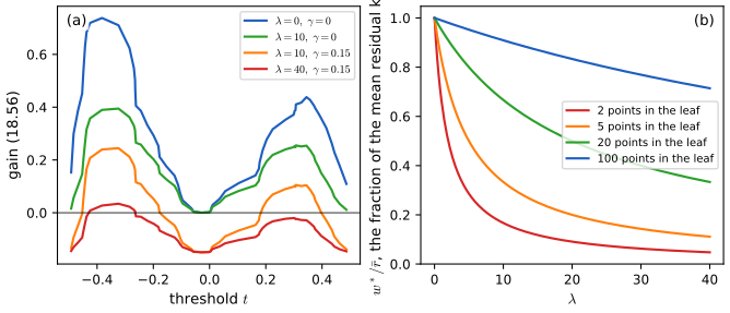
pp. 619–620 XGBoost (Chen and Guestrin, 2016) is an efficient implementation of gradient boosted trees with three statistical additions: a penalty on the tree, a second-order approximation of the loss (Friedman et al., 2000), and random feature subsets at nodes; plus engineering for scale (out-of-core computation, approximate split finding that avoids sorting). It minimises the regularised objective \[ L(f)=\sum_{i=1}^N\ell(y_i,f(\bm x_i))+\Omega(f),\qquad\Omega(f)=\gamma J+\tfrac12\lambda\sum_{j=1}^Jw_j^2, \tag{18.46, 18.47} \] with \(J\) leaves, leaf weights \(w_j\) and \(\gamma,\lambda\ge0\). At step \(m\) a second-order Taylor expansion of the loss at \(f_{m-1}\) gives \[ L_m(F_m)\approx\sum_{i}\Big[\ell(y_i,f_{m-1}(\bm x_i))+g_{im}F_m(\bm x_i)+\tfrac12h_{im}F_m(\bm x_i)^2\Big]+\Omega(F_m),\qquad h_{im}=\frac{\partial^2\ell(y_i,f(\bm x_i))}{\partial f(\bm x_i)^2}\Big|_{f_{m-1}}, \tag{18.49, 18.50} \] and for a tree \(F(\bm x)=w_{q(\bm x)}\) (\(q\) assigns a leaf), with \(G_{jm}=\sum_{i\in I_j}g_{im}\) and \(H_{jm}=\sum_{i\in I_j}h_{im}\), \[ L_m(q,\bm w)=\sum_{j=1}^J\Big[G_{jm}w_j+\tfrac12(H_{jm}+\lambda)w_j^2\Big]+\gamma J,\qquad w_j^*=-\frac{G_{jm}}{H_{jm}+\lambda}, \tag{18.53, 18.54} \] \[ L_m(q,\bm w^*)=-\frac12\sum_{j=1}^J\frac{G_{jm}^2}{H_{jm}+\lambda}+\gamma J,\qquad\text{gain}=\frac12\Big[\frac{G_L^2}{H_L+\lambda}+\frac{G_R^2}{H_R+\lambda}-\frac{(G_L+G_R)^2}{H_L+H_R+\lambda}\Big]-\gamma. \tag{18.55, 18.56} \] A split is worthwhile only if its gain is positive: the first term must exceed \(\gamma\).
Filling the gap 18.17: the XGBoost objective, leaf weights and gain, and their special cases pp. 619–620, (18.46)–(18.56)
Derivation
Taylor expansion and grouping by leaf. Expanding \(\ell(y_i,f_{m-1}+F)=\ell(y_i,f_{m-1})+g_{im}F+\frac12h_{im}F^2+O(F^3)\) gives (18.49); the first term does not depend on \(F_m\) and is dropped. For a tree, \(F_m(\bm x_i)=w_{q(\bm x_i)}\), so summing over the examples of each leaf \(I_j=\{i:q(\bm x_i)=j\}\), \(\sum_{i\in I_j}[g_iw_j+\frac12h_iw_j^2]=G_jw_j+\frac12H_jw_j^2\), and the penalty contributes \(\gamma J+\frac12\lambda\sum_jw_j^2\), which is (18.51)–(18.53).
Optimal weights. Each leaf is an independent quadratic \(G_jw+\frac12(H_j+\lambda)w^2\); when \(H_j+\lambda>0\) its minimiser is \(w_j^*=-G_j/(H_j+\lambda)\) (18.54) and its minimum is \(-\frac12G_j^2/(H_j+\lambda)\), giving (18.55). The leaf weight is a Newton step \(-G/H\) shrunk by \(\lambda\): for a leaf with \(n\) points and \(h=1\) (squared loss) the weight is \(\bar r\cdot n/(n+\lambda)\) where \(\bar r\) is the mean negative gradient, so a small leaf is shrunk more (Figure 18.S4b; checked: the code's leaf weights equal \(n/(n+\lambda)\) times the mean residual).
The gain. Splitting a leaf with \((G,H)\) into \((G_L,H_L)\) and \((G_R,H_R)\), \(G=G_L+G_R\), \(H=H_L+H_R\), replaces its term \(-\frac12G^2/(H+\lambda)+\gamma\) in (18.55) by \(-\frac12G_L^2/(H_L+\lambda)-\frac12G_R^2/(H_R+\lambda)+2\gamma\). The reduction in the objective is the difference: \(\frac12[\frac{G_L^2}{H_L+\lambda}+\frac{G_R^2}{H_R+\lambda}-\frac{G^2}{H+\lambda}]-\gamma\), which is (18.56). (The code compares this formula with the objective difference computed from (18.55) on random statistics: they agree to \(10^{-12}\).) The penalty \(\gamma\) per leaf is the price of the extra leaf, so splits with gain \(\le0\) are not made; this is a form of pre-pruning, and a split with negative gain can still be useful if it enables a good split below it, which a greedy rule misses (as in XOR).
Special cases. (i) Squared error \(\ell=\frac12(y-f)^2\), \(\lambda=\gamma=0\): \(g_i=f-y_i=-r_i\), \(h_i=1\). Leaf weight \(=\bar r\) (the least-squares boosting leaf), and the gain is \(\frac12\sum G^2/H\) differences \(=\frac12[\frac{(\sum_Lr)^2}{N_L}+\frac{(\sum_Rr)^2}{N_R}-\frac{(\sum r)^2}{N}]=\frac12\frac{N_LN_R}{N}(\bar r_L-\bar r_R)^2\), the least-squares gain of gap 18.2 (half the SSE reduction): the same tree as an ordinary regression tree (confirmed to \(10^{-9}\) on the 100-point data). (ii) Logistic loss, \(g_i=\pi_i-y_i\), \(h_i=\pi_i(1-\pi_i)\), \(\lambda=0\): leaf weight \(\sum(y_i-\pi_i)/\sum\pi_i(1-\pi_i)\), the Newton leaf of gap 18.16 and the LogitBoost step of gap 18.14. (iii) \(\lambda>0\) is a ridge penalty on the leaf weights (shrinkage); \(\gamma>0\) is a complexity penalty: with squared loss on the 100-point data a depth-4 tree has 16, 15, 10 and 6 leaves for \(\gamma=0,0.001,0.01,0.1\) (Figure 18.S4a shows the gain against the threshold). \(\square\)
See also: Elements of Statistical Learning, 10.10 gradient boosting, 10.12 regularization (shrinkage, subsampling); Introduction to Statistical Learning, 8.2.3 boosting; Bayesian and Probabilistic ML, 14.3.2 error functions for boosting; demos gradient boosting, boosting on the Hitters data.
18.6 Interpreting tree ensembles
pp. 620–623 A single tree is readable; an ensemble of hundreds is not. Two simple devices recover some of the interpretability: a ranking of the features by how much they contribute to the fit, and plots of the fitted function against one or two features with the others averaged out.
18.6.1 Feature importance
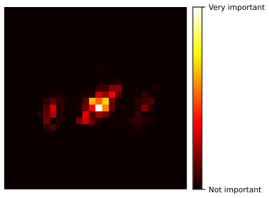
p. 621 For one tree \(T\), Breiman et al. (1984) define the importance of feature \(k\) as the total gain of the internal nodes that split on it, \[ R_k(T)=\sum_{j=1}^{J-1}G_j\,\ind(v_j=k), \tag{18.57} \] where \(G_j\) is the improvement (reduction in cost) at node \(j\) and \(v_j\) its feature. Averaging over the trees of an ensemble gives a steadier estimate, \(R_k=\frac1M\sum_{m}R_k(T_m)\) (18.58), usually rescaled so that the largest is 100%. Figure 18.8 does this for a forest that tells MNIST 0s from 8s, Figure 18.9 for a boosted classifier on the spam data.
Filling the gap 18.18: what (18.57) measures, and its biases p. 621, (18.57), (18.58)
Derivation
A decomposition of the training cost. Let \(r(t)\) be the cost of node \(t\) treated as a leaf (the weighted impurity or SSE) and \(G_t=r(t)-r(t_L)-r(t_R)\) the gain of the split at an internal node \(t\). Each non-root node is the child of exactly one internal node, so \(\sum_{t\text{ internal}}G_t=\sum_{t\text{ internal}}r(t)-\sum_{t\ne\text{root}}r(t)=r(\text{root})-\sum_{\ell\text{ leaf}}r(\ell)\): the sum telescopes. So the importances of a tree add up to the total reduction in training cost, \(\sum_kR_k(T)=r(\text{root})-\sum_\ell r(\ell)\) (confirmed numerically), and the normalised value \(R_k/\sum_{k'}R_{k'}\) is the share of that reduction due to splits on feature \(k\). For the Gini cost it equals the "mean decrease in impurity" and the normalised values equal the feature_importances_ of scikit-learn trees (confirmed on tie-free data). Averaging over trees (18.58) divides the variance, as for predictions; for boosting, the regression trees are fitted to the pseudo-residuals and the gain is the squared-error improvement, which is Friedman's measure.
Bias towards features with many split points. A feature with \(K\) distinct values offers \(K-1\) candidate splits. Under the null hypothesis that the feature is unrelated to the class, the gain of one fixed split, per example and for the entropy cost, is \(G^2/(2N)\) with \(G^2\) approximately \(\chi^2_{C-1}\) (gap 18.3); the learner takes the largest of the \(K-1\) correlated statistics, whose expectation grows with \(K\) (a maximally selected statistic; Strobl et al., 2007). A pure-noise continuous feature therefore looks better than a noise binary feature, and may look better than a weakly informative binary feature. In a simulation with 1000 observations and a forest of 100 trees (30 repetitions) the mean impurity importance was 0.159 for an informative binary feature, 0.023 for a noise binary feature, 0.131 for a noise feature with 10 values and 0.687 for a noise continuous feature: the pure noise gets four times the credit of the real signal. Permutation importance (Breiman, 2001) avoids this: permute the values of feature \(k\) in held-out data and record how much the error rises. In the same simulation it was 0.096 for the informative feature and 0.002, 0.001 and 0.001 for the three noise features (Figure 18.S6).
Other cautions. Importance has no sign: it says that the feature matters, not in which direction (the partial dependence plots of Section 18.6.2 do that; in the spam example the presence or absence of a word can be what counts). Correlated features share credit in an arbitrary way: of two identical features the learner picks one at each node, and which one is chosen depends on tie-breaking or on the random subset. The importance is computed on the training data and measures what the model uses, not what generalises. \(\square\)
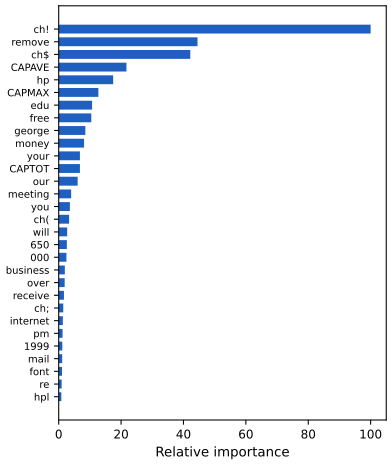
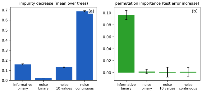
18.6.2 Partial dependency plots
p. 623 Having found the relevant features, one asks how they affect the output. The partial dependence on feature \(k\) is \[ \bar f_k(x_k)=\frac1N\sum_{n=1}^Nf(\bm x_{n,-k},x_k), \tag{18.59} \] the fitted function with feature \(k\) set to \(x_k\) in every training example and the other features left as they are, averaged: a marginalisation of the others. For a binary classifier the values are plotted as log-odds. Interactions between two features \(j,k\) are shown by the joint version \(\bar f_{jk}(x_j,x_k)=\frac1N\sum_nf(\bm x_{n,-jk},x_j,x_k)\) (18.60). Figure 18.10 shows both for the spam model: the log-odds of spam rise with the frequency of "!" and "remove" and fall with that of "edu" and "hp", and at a given frequency of "!" the log-odds of spam are much higher when "hp" is absent.
Filling the gap 18.19: what the partial dependence function is, what it hides and what it shows p. 623, (18.59), (18.60)
Derivation
It estimates a marginalised function. Let \(\bm X_{-k}\) be the other features. \(\bar f_k(x_k)\) is the Monte Carlo estimate, with the training examples as draws, of \(\E_{\bm X_{-k}}[f(x_k,\bm X_{-k})]\): the expectation under the marginal distribution of the other features, not the conditional one given \(x_k\). The conditional version \(\E[f(\bm X)\given X_k=x_k]\) would also pick up the effect of features correlated with \(X_k\); the partial dependence isolates the effect of changing \(x_k\) alone, at the price of evaluating \(f\) at combinations that may be unlikely (or impossible) in the data when features are correlated.
Additive models. If \(f(\bm x)=f_k(x_k)+f_{-k}(\bm x_{-k})\) then \(\bar f_k(x_k)=f_k(x_k)+\frac1N\sum_nf_{-k}(\bm x_{n,-k})=f_k(x_k)+\mathrm{const}\): the partial dependence recovers the component up to an additive constant. (Numerically for \(\sin3x_1+x_2^2\) with 3000 points the curve for \(x_1\) matches \(\sin3x_1\) up to a constant to 0.03.)
Interactions. If \(f(x_1,x_2)=x_1x_2\) with \(x_2\) symmetric about 0 then \(\bar f_1(x_1)=x_1\cdot\frac1N\sum_nx_{n2}\approx0\): the one-dimensional partial dependence is flat although \(x_1\) matters a lot (the variance of \(f\) is entirely due to the interaction). Plotting the two-feature version (18.60) shows the saddle: with only two features it reproduces \(f\) exactly (Figure 18.S7). In general \(\bar f_{jk}-\bar f_j-\bar f_k+\mathrm{const}\) isolates the interaction of \(j\) and \(k\) up to the constants, and if it is small relative to the variation of \(\bar f_{jk}\), the pair acts additively (Friedman's \(H\) statistic). In the spam model the log-odds at "!" frequency 1 are +1.0 when "hp" is absent and \(-2.2\) when "hp" has frequency 1, against \(-2.4\) and \(-6.8\) at "!" frequency 0: the effect of "hp" is \(-4.3\) at "!" frequency 0 and \(-3.2\) at frequency 1, so the two features do not act additively.
Correlated features: a worked example (Exercise 18.8). For \(f=x_1+x_2^2+x_1x_2\) with \(x_2=\rho x_1+\sqrt{1-\rho^2}\varepsilon\) (both standard normal), the partial dependence is \(\bar f_1(x_1)=x_1+\E x_2^2+x_1\E x_2=x_1+1\) whereas \(\E[f\given x_1]=x_1+(\rho+\rho^2)x_1^2+1-\rho^2\), which for \(\rho=0.8\) is \(x_1+1.44x_1^2+0.36\). The two answer different questions, and neither is "the" effect of \(x_1\).
Log-odds and trees. For a boosted classifier the code averages the model's log-odds \(f\) over the data, as is usual (averaging the probabilities and then taking the log-odds gives a different curve). For a tree ensemble the average can be computed without a pass over the data by a weighted traversal of each tree that follows both branches of a split on a feature not in the plot, weighting them by the fraction of training examples that fell each way. The implementation here uses the brute-force definition (18.59), and matches the brute-force routine of scikit-learn to \(10^{-8}\). \(\square\)
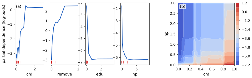
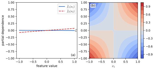
See also: Elements of Statistical Learning, 10.13 interpretation, 15.3.2 variable importance; demos random forest importance, spam partial dependence (Elements of Statistical Learning).
18.7 Exercises
The draft of Chapter 18 has no end-of-chapter exercises. The eight problems below are my own, in the style of the other chapters, covering what the chapter teaches: node costs, a worked regression tree, voting, the bootstrap and bagging variance, AdaBoost and XGBoost by hand, leaf values and partial dependence. Each has a complete solution (hidden); the numerical ones were also solved by the code.
Exercise 18.1 (impurity measures disagree). A node holds 400 examples of each of two classes. Split A sends (300, 100) to the left and (100, 300) to the right; split B sends (200, 400) left and (200, 0) right. (a) Compute the decrease in the misclassification rate, the Gini index and the entropy (bits) for each split, children weighted by their sizes. (b) Which split does each criterion prefer, and why do you think Gini and entropy are preferred for growing? (c) Give a node and a split for which the misclassification rate does not decrease although the split is useful.
Solution
(a) The parent has proportions (\(\frac12,\frac12\)): misclassification \(0.5\), Gini \(1-\frac14-\frac14=0.5\), entropy 1 bit. Split A: both children have proportions (0.75, 0.25): misclassification 0.25, Gini \(1-0.5625-0.0625=0.375\), entropy \(-0.75\log_20.75-0.25\log_20.25=0.8113\); they have equal size, so the weighted values are the same: decreases \(0.5-0.25=0.25\), \(0.5-0.375=0.125\), \(1-0.8113=0.1887\). Split B: the left child (600 of 800 examples) has proportions (\(\frac13,\frac23\)): misclassification \(\frac13\), Gini \(1-\frac19-\frac49=\frac49\), entropy 0.9183; the right child (200) is pure with impurity 0. Weighted: misclassification \(0.75\cdot\frac13=0.25\), Gini \(0.75\cdot\frac49=\frac13\), entropy \(0.75\cdot0.9183=0.6887\). Decreases: \(0.25\), \(0.5-0.3333=0.1667\), \(1-0.6887=0.3113\).
(b) The misclassification rate ties them (both decrease by 0.25: both leave 200 errors out of 800). Gini and entropy both prefer B: A reduces the Gini index by 0.125 and B by 0.167, the entropy by 0.189 and 0.311 bits. B creates a pure leaf, which is a better starting point for further splits (the remaining node can still be split, whereas A leaves two mixed children each at 25% error that need further splits); the concave impurities reward purity. The misclassification rate is piecewise linear, so it is blind to how the errors are distributed between the children (gap 18.3).
(c) A node with (300, 100) split into (200, 50) and (100, 50): all three nodes predict the majority class, the error stays at 100 of 400 so the misclassification gain is 0, yet the Gini cost falls from 150 to 146.7 and the split separates a region with 80% positives from one with 67% positives. (Confirmed by the code: the three gains are \(0\), \(3.33\) and positive for the entropy.) \(\square\)
Exercise 18.2 (a regression tree by hand). The data are \(x=1,\dots,6\) with \(y=(1,2,1.5,6,7,5.5)\). (a) Compute the sum of squares at the root and the child costs of every possible first split, and find the best. (b) Grow the tree to depth 2 (squared error, greedy) and give the leaf values. (c) Check the gain of the first split with the formula \(\frac{N_LN_R}N(\bar y_L-\bar y_R)^2\) of gap 18.2.
Solution
(a) \(\bar y=23/6=3.8333\), \(\sum y^2=122.5\), so the root SSE is \(122.5-23^2/6=34.333\). The thresholds lie between consecutive \(x\) values; the total child SSE after splitting after position \(s=1,\dots,5\) is \(24.7,\ 18.0,\ 1.667,\ 16.81,\ 31.0\). The best split is after \(x=3\) (threshold 3.5): left \(\{1,2,1.5\}\) has mean 1.5 and SSE 0.5, right \(\{6,7,5.5\}\) has mean 6.1667 and SSE 1.1667, total 1.667; the gain is \(34.333-1.667=32.667\).
(b) The left node holds \(x=1,2,3\) with \(y=(1,2,1.5)\) and SSE 0.5. Splitting after \(x=1\) gives \(\{1\}\,|\,\{2,1.5\}\) with SSE \(0+0.125\), a gain of \(0.375\); splitting after \(x=2\) gives \(\{1,2\}\,|\,\{1.5\}\) with SSE 0.5, no gain. So the left node splits at threshold 1.5 with leaf values 1 and 1.75. The right node holds \(x=4,5,6\) with \(y=(6,7,5.5)\) and SSE 1.1667: \(\{6,7\}\,|\,\{5.5\}\) (threshold 5.5) leaves SSE \(0.5+0\), a gain of \(0.667\), whereas \(\{6\}\,|\,\{7,5.5\}\) leaves 1.125; so it splits at 5.5 with leaf values 6.5 and 5.5. The tree has four leaves with values 1, 1.75, 6.5, 5.5 and training SSE \(0.125+0.5=0.625\).
(c) \(\frac{3\cdot3}6(6.1667-1.5)^2=1.5\cdot21.78=32.667\), as in (a). The code returns the same thresholds, values and gains. \(\square\)
Exercise 18.3 (how many voters?). (a) Using the normal approximation to (18.11), find the number \(M\) of independent voters, each correct with probability \(\theta\), needed for a majority to be correct with probability 0.99, for \(\theta=0.55\) and \(0.60\); compare with the exact binomial computation. (b) Now let the voters be conditionally independent given an accuracy \(\Theta\sim\operatorname{Beta}(5.5,4.5)\) (mean 0.55). What is the best accuracy the majority vote can reach as \(M\to\infty\), and what is the correlation of two votes?
Solution
(a) \(p\approx\Phi(\sqrt M(2\theta-1)/(2\sqrt{\theta(1-\theta)}))\ge0.99\) needs the argument \(\ge z_{0.99}=2.326\), i.e. \(M\ge\big(2.326\cdot2\sqrt{\theta(1-\theta)}/(2\theta-1)\big)^2\). For \(\theta=0.55\): \(2\sqrt{0.2475}=0.995\), so \(M\ge(2.326\cdot0.995/0.1)^2=535.6\), about 536; the exact binomial computation gives 539 (odd \(M\)). For \(\theta=0.60\): \(2\sqrt{0.24}=0.9798\), \(M\ge(2.326\cdot0.9798/0.2)^2=129.8\), about 130; exact 133. The approximation is within 1–3%, and a much larger advantage needs far fewer voters: \(M\propto(\theta-\frac12)^{-2}\).
(b) By gap 18.7, \(\lim_M\Pr(\text{majority correct})=\Pr(\Theta>\frac12)=1-I_{1/2}(5.5,4.5)=0.629\) (regularised incomplete beta function), no matter how many voters. The votes have \(\operatorname{cov}(Y_1,Y_2)=\operatorname{var}\Theta=\frac{ab}{(a+b)^2(a+b+1)}=\frac{24.75}{100\cdot11}=0.0225\) and \(\operatorname{var}Y=0.55\cdot0.45=0.2475\), so \(\rho=0.0225/0.2475=0.0909=1/(a+b+1)\). A correlation of 0.09 already caps the committee at 63% accuracy against the 99% of 539 independent voters. \(\square\)
Exercise 18.4 (bootstrap and bagging). (a) For a data set of \(N=20\) examples, find the probability that a given example is missing from a bootstrap sample, the expected number of distinct examples in it, and compare with \(e^{-1}\) and 63.2%. (b) Show that the number of times a given example appears in a bootstrap sample is \(\operatorname{Bin}(N,1/N)\), with mean 1 and variance \(1-1/N\). (c) If bagged trees have pairwise correlation \(\rho=0.4\), how many trees are needed for the variance to be within 10% of its floor \(\rho\sigma^2\)?
Solution
(a) \((1-\frac1{20})^{20}=0.95^{20}=0.3585\) (against \(e^{-1}=0.3679\)); the expected number of distinct examples is \(20(1-0.3585)=12.83\), a fraction 0.6415 (against 0.632). The finite-\(N\) values differ because \((1-1/N)^N\) increases to \(e^{-1}\) (gap 18.9).
(b) Each of the \(N\) draws picks the given example independently with probability \(1/N\), so the count is binomial with parameters \(N\) and \(1/N\): mean \(N\cdot\frac1N=1\), variance \(N\cdot\frac1N(1-\frac1N)=1-\frac1N\). For large \(N\) it is approximately Poisson(1), which has \(\Pr(0)=e^{-1}\).
(c) The variance \(\rho\sigma^2+(1-\rho)\sigma^2/B\le1.1\rho\sigma^2\) iff \((1-\rho)/B\le0.1\rho\) iff \(B\ge(1-\rho)/(0.1\rho)=0.6/0.04=15\). With 14 trees the variance exceeds 1.1 times the floor (\(0.4+0.6/14=0.4429>0.44\)), with 15 trees it is exactly 1.1 times the floor. So beyond about 15 trees a correlation-0.4 ensemble gains almost nothing more; to go lower one must reduce \(\rho\) (random forests). \(\square\)
Exercise 18.5 (AdaBoost by hand). Ten points \(x=1,\dots,10\) have labels \(\tilde y=(+,+,+,-,-,-,+,+,-,-)\). The weak learners are stumps \(\pm\sgn(x-t)\) with thresholds halfway between integers. Run three rounds of AdaBoost (Algorithm 18.1): give the stump, its weighted error \(\operatorname{err}_m\), \(\alpha_m\) and the new weights at each round, the training error of \(\sgn\sum_m\alpha_mF_m\) after each round, and the exponential loss \(\frac1N\sum_ie^{-\tilde y_if(\bm x_i)}\) with \(f=\frac12\sum\alpha_mF_m\).
Solution
Round 1 (all weights 0.1). The best stump predicts \(+\) for \(x\le3.5\) and \(-\) beyond; it errs at \(x=7,8\): \(\operatorname{err}_1=0.2\), \(\alpha_1=\ln4=1.3863\). The weights of \(x=7,8\) are multiplied by 4 (0.4), the others stay at 0.1; the total is 1.6 so the normalised weights are 0.25 on \(x=7,8\) and 0.0625 elsewhere. (The weighted error of this stump under the new weights is \(2\cdot0.25=0.5\), as it must be: gap 18.13.) Training error of \(\sgn(\alpha_1F_1)\): 0.2; exponential loss \(\sqrt{4\cdot0.2\cdot0.8}=0.8\).
Round 2. The best stump predicts \(+\) for \(x\le8.5\) and \(-\) beyond; it errs at \(x=4,5,6\): \(\operatorname{err}_2=3\cdot0.0625=0.1875\), \(\alpha_2=\ln(0.8125/0.1875)=1.4663\). Multiplying the weights of \(x=4,5,6\) by 4.333 gives \(0.2708\); the total is 1.625; the new weights are 0.1667 on \(x=4,5,6\), 0.1538 on \(x=7,8\) and 0.0385 on \(x=1,2,3,9,10\). Ensemble \(\sgn(1.3863F_1+1.4663F_2)\): for \(x=4,5,6\) the sum is \(-1.3863+1.4663=+0.08>0\), wrong: training error 0.3 (it increases; boosting only guarantees the exponential loss falls). Exponential loss \(0.8\cdot2\sqrt{0.1875\cdot0.8125}=0.6245\).
Round 3. The best stump predicts \(-\) for \(x\le6.5\) and \(+\) beyond, with errors at \(x=1,2,3\) (weight \(0.0385\) each) and \(x=9,10\) (\(0.0385\) each): \(\operatorname{err}_3=0.1923\), \(\alpha_3=\ln(0.8077/0.1923)=1.4351\). The ensemble has \(f=1.3863s_1+1.4663s_2+1.4351s_3\) (\(s_1=+1\) for \(x\le3.5\), \(s_2=+1\) for \(x\le8.5\), \(s_3=-1\) for \(x\le6.5\)): for \(x=1,2,3\): \(+1.4175\); \(x=4,5,6\): \(-1.3551\); \(x=7,8\): \(+1.5151\); \(x=9,10\): \(-1.4175\). All ten signs are correct: training error 0. Exponential loss \(0.6245\cdot2\sqrt{0.1923\cdot0.8077}=0.4922\), equal to the mean of \(e^{-\tilde yf/2}\) computed directly, and above the training error in every round (0.2, 0.3, 0): gap 18.12. (Solved by the code with identical numbers.) \(\square\)
Exercise 18.6 (an XGBoost split by hand). At some round of boosting six training examples, sorted by one feature, have gradients \(g=(-2,-1.5,-1,1,1.5,2.5)\) and Hessians \(h_i=1\); take \(\lambda=1,\gamma=0.5\). (a) What leaf weight would a single leaf containing all six get? (b) Find the best split of the six into two leaves using (18.56), and the leaf weights. (c) For which \(\gamma\) would this split not be made?
Solution
(a) \(G=0.5\), \(H=6\), \(w^*=-G/(H+\lambda)=-0.5/7=-0.0714\).
(b) With \(\lambda=1\): the parent term \(G^2/(H+\lambda)=0.25/7=0.0357\). Splits after \(1,\dots,5\) examples: after 2: \(G_L=-3.5,H_L=2\): \(12.25/3=4.083\); \(G_R=4,H_R=4\): \(16/5=3.2\); gain \(\frac12(4.083+3.2-0.0357)-0.5=3.124\). After 3: \(G_L=-4.5,H_L=3\): \(20.25/4=5.0625\); \(G_R=5,H_R=3\): \(25/4=6.25\); gain \(\frac12(5.0625+6.25-0.0357)-0.5=5.138\). After 4: \(G_L=-3.5,H_L=4\): \(12.25/5=2.45\); \(G_R=4,H_R=2\): \(5.333\); gain \(3.374\). (After 1 and 5 the gains are 1.003 and 1.378.) The best split is after three examples, gain 5.138. Leaf weights \(w_L^*=4.5/4=1.125\), \(w_R^*=-5/4=-1.25\): the left leaf (negative gradients) moves its predictions up, the right leaf down.
(c) The split is made iff the gain is positive: \(\gamma<\frac12(5.0625+6.25-0.0357)=5.638\). So \(\gamma=0.5\) is far below the threshold, and \(\gamma\ge5.64\) removes the split altogether. (Matches the code.) \(\square\)
Exercise 18.7 (leaf values). (a) Prove that the minimiser over \(w\) of \(\sum_{i=1}^n|r_i-w|\) is a median of the \(r_i\), and that the minimiser of \(\sum_i(r_i-w)^2\) is the mean. (b) For the residuals \(r=(-1,0.2,0.4,3)\) in one leaf give the leaf values for squared, absolute and Huber (\(\delta=1\), one step from the median) loss, and the pseudo-residuals the tree is grown on for the absolute loss. (c) Show that for the log loss the one-step Newton leaf value is \(\sum_i(y_i-p_i)/\sum_ip_i(1-p_i)\).
Solution
(a) Squared: the derivative \(-2\sum(r_i-w)=0\) at \(w=\bar r\), a minimum since the second derivative is \(2n>0\). Absolute: sort the \(r_{(1)}\le\dots\le r_{(n)}\). The function \(\phi(w)=\sum|r_i-w|\) is convex and piecewise linear, with slope \(\#\{r_i<w\}-\#\{r_i>w\}\) away from the data points. For \(w\) below the median the slope is negative (more points above than below), above it positive, so the minimum is where the slope changes sign: at the median for odd \(n\), at any point between \(r_{(n/2)}\) and \(r_{(n/2+1)}\) for even \(n\).
(b) Mean: \(\bar r=(−1+0.2+0.4+3)/4=0.65\). Median: sorted \((-1,0.2,0.4,3)\), any value in \([0.2,0.4]\); the midpoint 0.3. Huber: \(\tilde r=0.3\); the clipped deviations are \(\operatorname{clip}(-1.3)=-1\), \(\operatorname{clip}(-0.1)=-0.1\), \(0.1\), \(\operatorname{clip}(2.7)=1\) with mean 0, so \(w=0.3\). The pseudo-residuals for the absolute loss are \(\sgn(r_i)=(-1,+1,+1,+1)\). The outlier 3 moves the mean from \(-0.133\) (the mean of \(-1,0.2,0.4\)) to 0.65, a shift of 0.78, but the median only from 0.2 to 0.3, a shift of 0.1: the median is robust.
(c) With \(\ell(y,f)=\log(1+e^f)-yf\): \(\ell'=\sigma(f)-y=p-y\) and \(\ell''=p(1-p)\). A Newton step on \(\sum_i\ell(y_i,f_i+w)\) from \(w=0\) is \(w=-\sum\ell'/\sum\ell''=\sum(y_i-p_i)/\sum p_i(1-p_i)\). \(\square\)
Exercise 18.8 (partial dependence with correlated features). Let \(f(x_1,x_2)=x_1+x_2^2+x_1x_2\), with \(x_1\sim\N(0,1)\) and \(x_2=\rho x_1+\sqrt{1-\rho^2}\,\varepsilon\), \(\varepsilon\sim\N(0,1)\) independent, \(\rho=0.8\). (a) Compute the population partial dependence \(\bar f_1(x_1)=\E_{x_2}[f(x_1,x_2)]\) (with \(x_2\) drawn from its marginal). (b) Compute the conditional expectation \(\E[f\given x_1]\). (c) Compare at \(x_1=2\).
Solution
(a) The marginal of \(x_2\) is \(\N(0,1)\) (variance \(\rho^2+1-\rho^2=1\)), so \(\E x_2=0\), \(\E x_2^2=1\) and \(\bar f_1(x_1)=x_1+1+x_1\cdot0=x_1+1\).
(b) Given \(x_1\), \(x_2\sim\N(\rho x_1,1-\rho^2)\): \(\E[x_2\given x_1]=\rho x_1\), \(\E[x_2^2\given x_1]=\rho^2x_1^2+1-\rho^2\). So \(\E[f\given x_1]=x_1+\rho^2x_1^2+1-\rho^2+\rho x_1^2=x_1+(\rho+\rho^2)x_1^2+1-\rho^2\), which for \(\rho=0.8\) is \(x_1+1.44x_1^2+0.36\).
(c) At \(x_1=2\): the partial dependence is 3; the conditional expectation is \(2+1.44\cdot4+0.36=8.12\). A simulation with 400,000 draws (conditioning on \(|x_1-2|<0.03\)) gives 8.26, and 3.00 for the partial dependence. The partial dependence holds \(x_2\) at its marginal distribution, in which \(x_1=2\) and \(x_2\) large are not linked; the conditional expectation includes the fact that when \(x_1=2\), \(x_2\) is typically near 1.6, where \(x_2^2\) and \(x_1x_2\) are large. Which one is "right" depends on the question: the first is the effect of intervening on \(x_1\) alone; the second is a prediction given \(x_1\). \(\square\)
Demonstrations
| Page | What it shows | In the notes |
|---|---|---|
| Growing a classification tree greedily | CART on the iris petals or on the XOR problem: Gini, entropy or misclassification, depth, smallest leaf and smallest worthwhile gain, the gain of every threshold at the root, and one observation left out. Presets: 1 Gini depth 2; 2 a point left out; 3 XOR, no split helps; 4 XOR without a bar on the gain; 5 entropy. | 18.1.2, 18.1.3, 18.1.5, gap 18.4, gap 18.6 |
| Bagging and random forests on two moons | A single tree, bagging and a random forest on 250 two-moons points: number of trees, training set size, features tried per split; the averaged surface, the test error and the out-of-bag error against the number of trees. Presets: 1 one tree; 2 bag of 10; 3 bag of 50; 4 forest m = 1; 5 60 training points. | 18.3, 18.4, gap 18.9, gap 18.10 |
| AdaBoost with decision stumps | Point weights, the weighted vote after M rounds, the training error, the exponential loss equal to the product of the round factors, the test error and the weighted error of each learner; stumps or deeper trees; flipped labels. Presets: 1 a single stump; 2 ten rounds; 3 150 rounds; 4 flipped labels; 5 depth-2 trees. | 18.5.3, 18.5.4, gap 18.12, gap 18.13, gap 18.14 |
| Gradient boosting of regression trees | Squared, absolute and regularised second-order (XGBoost) losses on a noisy curve with optional outliers; rounds, learning rate, depth, \(\lambda\) and \(\gamma\); the ensemble, the residuals with the latest tree and the error curves. Presets: 1 three rounds; 2 shrinkage; 3 overfitting; 4 outliers, absolute loss; 5 XGBoost penalty. | 18.5.2, 18.5.5, 18.5.5.2, gap 18.11, gap 18.15, gap 18.17 |
The Python code that produces every figure of this page is code/ch18_trees_forests_boosting.py (see the code index). The demonstrations share a small JavaScript tree learner, ch18-tree-kit.js. Companion demos on the same ideas: tree pruning, bagging trees, out-of-bag error, random forest decorrelation, AdaBoost, gradient boosting, random forest importance, spam partial dependence.
Notes on the book
Points where the book is imprecise or wrong
- Section 18.1.1, "\(J\) is the number of nodes". In \(\bm\theta=\{(R_j,w_j):j=1{:}J\}\) the index runs over the leaves; a binary tree with \(J\) leaves has \(2J-1\) nodes and \(J-1\) internal nodes, which is the range of the sum in (18.57) (gap 18.1).
- Figure 18.1a and the text after it, "\(x_3\le t_3\)". The third threshold of the example tree is on \(x_1\) (the tree has two inputs); the region is \(R_4=[(x_1\le t_1),(x_2>t_2),(x_1\le t_3)]\).
- Section 18.2, the value 0.97. For \(\theta=0.51\), \(M=10{,}000\) the probability (18.11) is 0.9767, which rounds to 0.98 (0.73 for \(M=1000\) is right: 0.7261). The calculation assumes independent voters; with a shared accuracy the limit is \(\Pr(\Theta>\frac12)\), not 1 (gap 18.7).
- Section 18.5, "bagging and RF reduce the variance by fitting independent trees". Bootstrap trees fitted to one data set are identically distributed but correlated (they share the data), and the variance of their average has the floor \(\rho\sigma^2\) (gap 18.9); random forests exist to lower \(\rho\).
- Section 18.5, "it can be shown ... the final ensemble will have higher accuracy than any given component". What can be shown is a bound on the training error, \(\prod_m2\sqrt{\epsilon_m(1-\epsilon_m)}\le e^{-2\sum_m\gamma_m^2}\), under the assumption that every learner beats chance on the re-weighted data; nothing follows for the test error without further (margin) arguments (gap 18.12).
- Table 18.1, exponential loss. The column headed \(-\partial\ell/\partial f\) shows \(-\tilde y_i\exp(-\tilde y_if)\); the negative gradient of \(\exp(-\tilde yf)\) is \(+\tilde y\exp(-\tilde yf)\) (gap 18.15).
- Table 18.1, binary log loss. The loss is printed as \(\log(1+e^{-\tilde y_if_i})\) with \(\pi_i=\sigma(2f_i)\) and the negative gradient as \(y_i-\pi_i\), which do not go together: for \(\log(1+e^{-\tilde yf})\) it is \(y-\sigma(f)\), for the loss (18.21), \(\log(1+e^{-2\tilde yf})\), it is \(2(y-\sigma(2f))\). (Also, Figure 18.7 plots \(\log_2(1+e^{-m})\) against the margin, i.e. (18.21) with the factor 2 removed and the logarithm in base 2.)
- Equation (18.23). The expected loss is written with \(f(x)\) where \(F(x)\) is meant.
- Algorithms 18.1 and 18.2. Line 3 of Algorithm 18.1 writes the weights as \(w\) but they are \(\omega\) elsewhere; in Algorithm 18.2 the initial weights \(\omega_i=1/N\) are overwritten in step 4 before use, and the working response must be clipped (and the weights floored) in practice, because \(z_i\) is unbounded as \(\pi_i\to0\) or 1.
- Section 18.1.5 and Figure 18.3, "omitting even a single data point ... dramatically different". It can happen (a tie in a small leaf, or two splits with nearly equal gain), but it did not in my runs: for the depth-3 iris tree 4% of single deletions change the partition at all, by 0.2% of the plane on average; for the full two-moons tree the mean change is 0.3%. The instability that matters for bagging is under bootstrap resampling, where two trees disagree on 11–17% of the plane (gap 18.6).
- Section 18.4, "... because many input features are irrelevant". In my replication the forest (\(m=7\)) beats bagged trees on the spam data (0.046 against 0.062), but the mechanism proved here is the lower correlation of the trees (gap 18.10), which does not need irrelevant features; whether irrelevant features also matter is not tested by the book's figure.
- Figure 18.9 caption. "The dataset has X training examples with Y features" leaves placeholders unfilled; the text of Section 18.4 gives 4601 e-mails with 57 features (3065 for training in the usual split).
- Section 18.1.2, the threshold set. Taking \(\mathcal T_j\) to be all distinct values and testing \(x\le t\) includes the largest value, which sends every example left and gives an empty right child; harmless, but only the first \(n-1\) values define distinct partitions.
References
- Murphy, K. P. (2022). Probabilistic Machine Learning: An Introduction. MIT Press, Cambridge, MA. Chapter 18, pp. 603–623. probml.github.io/pml-book/book1.html.
- Breiman, L. (1996). Bagging predictors. Machine Learning, 24(2), 123–140.
- Breiman, L. (2001). Random forests. Machine Learning, 45(1), 5–32.
- Breiman, L., Friedman, J. H., Olshen, R. A. and Stone, C. J. (1984). Classification and Regression Trees. Wadsworth, Belmont, CA.
- Bühlmann, P. and Hothorn, T. (2007). Boosting algorithms: regularization, prediction and model fitting. Statistical Science, 22(4), 477–505.
- Bühlmann, P. and Yu, B. (2003). Boosting with the \(L_2\) loss: regression and classification. Journal of the American Statistical Association, 98(462), 324–339.
- Chen, T. and Guestrin, C. (2016). XGBoost: a scalable tree boosting system. Proceedings of the 22nd ACM SIGKDD International Conference on Knowledge Discovery and Data Mining, 785–794.
- Efron, B., Hastie, T., Johnstone, I. and Tibshirani, R. (2004). Least angle regression. Annals of Statistics, 32(2), 407–499.
- Fisher, R. A. (1936). The use of multiple measurements in taxonomic problems. Annals of Eugenics, 7(2), 179–188.
- Freund, Y. and Schapire, R. E. (1996). Experiments with a new boosting algorithm. Proceedings of the 13th International Conference on Machine Learning, 148–156.
- Friedman, J. H. (1999). Stochastic gradient boosting. Technical report, Stanford University.
- Friedman, J. H. (2001). Greedy function approximation: a gradient boosting machine. Annals of Statistics, 29(5), 1189–1232.
- Friedman, J. H., Hastie, T. and Tibshirani, R. (2000). Additive logistic regression: a statistical view of boosting. Annals of Statistics, 28(2), 337–407.
- Friedman, J. H. and Meulman, J. J. (2003). Multiple additive regression trees with application in epidemiology. Statistics in Medicine, 22(9), 1365–1381.
- Grandvalet, Y. (2004). Bagging equalizes influence. Machine Learning, 55(3), 251–270.
- Hastie, T., Tibshirani, R. and Friedman, J. (2009). The Elements of Statistical Learning, 2nd edition. Springer, New York.
- Hyafil, L. and Rivest, R. L. (1976). Constructing optimal binary decision trees is NP-complete. Information Processing Letters, 5(1), 15–17.
- Mason, L., Baxter, J., Bartlett, P. and Frean, M. (2000). Boosting algorithms as gradient descent. Advances in Neural Information Processing Systems, 12.
- Minka, T. P. (2000). Bayesian model averaging is not model combination. Technical note, MIT Media Lab.
- Nakkiran, P., Neyshabur, B. and Sedghi, H. (2020). The deep bootstrap framework: good online learners are good offline generalizers. Preprint (later published at the International Conference on Learning Representations, 2021).
- Quinlan, J. R. (1986). Induction of decision trees. Machine Learning, 1(1), 81–106.
- Quinlan, J. R. (1993). C4.5: Programs for Machine Learning. Morgan Kaufmann, San Mateo, CA.
- Schapire, R. E. and Freund, Y. (2012). Boosting: Foundations and Algorithms. MIT Press, Cambridge, MA.
- Schapire, R. E. (1990). The strength of weak learnability. Machine Learning, 5(2), 197–227.
- Schapire, R. E., Freund, Y., Bartlett, P. and Lee, W. S. (1998). Boosting the margin: a new explanation for the effectiveness of voting methods. Annals of Statistics, 26(5), 1651–1686.
- Suárez, A. and Lutsko, J. F. (1999). Globally optimal fuzzy decision trees for classification and regression. IEEE Transactions on Pattern Analysis and Machine Intelligence, 21(12), 1297–1311.
- Strobl, C., Boulesteix, A.-L., Zeileis, A. and Hothorn, T. (2007). Bias in random forest variable importance measures: illustrations, sources and a solution. BMC Bioinformatics, 8, 25.
- Wolpert, D. H. (1992). Stacked generalization. Neural Networks, 5(2), 241–259.
- Zhu, J., Zou, H., Rosset, S. and Hastie, T. (2009). Multi-class AdaBoost. Statistics and Its Interface, 2(3), 349–360.
The numerical statements in the text (the node costs and their identities, the split search, the monotone invariance, pruning against a library, the voting probabilities, the bootstrap and bagging variance formulas, the AdaBoost identities and bound, the Newton form of LogitBoost, the gradients of Table 18.1, gradient boosting and the XGBoost formulas against library implementations, importance and partial dependence, and the numerical answers to the exercises) were confirmed numerically.