Multiple Testing
One hypothesis test at level 0.05 is wrong, when the null hypothesis holds, one time in twenty. Run two thousand tests and about a hundred true null hypotheses will be rejected by chance. This chapter is about keeping such false discoveries in check. The family-wise error rate asks that there be none at all, with high probability (Bonferroni, Holm, Tukey, Scheffé); the false discovery rate asks only that they be a small share of the discoveries (Benjamini–Hochberg). When the textbook null distribution of a statistic is in doubt, random relabelling of the data supplies one. The Fund data (2,000 fund managers) and the Khan gene expression data (2,308 genes) run through the chapter and its lab.
Ch. 1 Introduction Ch. 2 Statistical learning Ch. 3 Linear regression Ch. 4 Classification Ch. 5 Resampling Ch. 6 Selection and regularization Ch. 7 Beyond linearity Ch. 8 Trees Ch. 9 SVMs Ch. 10 Deep learning Ch. 11 Survival analysis Ch. 12 Unsupervised learning Ch. 13 Multiple testing
How to read these notes
They follow the book. Sections carry the book's numbers (13.1, 13.3.2, ...) and displayed equations that appear in the book carry its numbers, e.g. \((13.5)\). Both editions share the text, figures and exercises of this chapter; page numbers are those of the R edition (the Python edition's are four higher in Sections 13.1–13.5).
Filling the gaps. The book states several results without proof: that rejecting when \(p\le\alpha\) controls the Type I error, that Holm's procedure controls the family-wise error rate ("slightly more complicated" than Bonferroni), and that Benjamini–Hochberg controls the false discovery rate ("well beyond the scope of this book"). An orange Filling the gap box gives each argument, short but complete. Derivations start hidden: open one with its bar, or use the button below.
The lab in two languages. Section 13.6 shows each lab step in R (left) and Python (right), with the numbers each produces, and marks where and why the two differ. The code is that of ch13_lab.R and ch13_lab.py; the figures come from ch13_multiple_testing.py.
Main reference
G. James, D. Witten, T. Hastie and R. Tibshirani, An Introduction to Statistical Learning with Applications in R, 2nd edition, Springer (2021), Chapter 13, pages 553–595; and G. James, D. Witten, T. Hastie, R. Tibshirani and J. Taylor, An Introduction to Statistical Learning with Applications in Python, Springer (2023), Chapter 13, pages 557–596. Book website, with the data sets: www.statlearning.com. Further reading is listed in the references.
The explanations, derivations, figures and code are my own; equations are cited by their numbers in the book.
Companion courses
- Statistical Learning: Theory and Methods (the graduate course on the same authors' Elements of Statistical Learning) treats multiple testing in Section 18.7: Bonferroni (Result 18.11), the Benjamini–Hochberg procedure and its FDR control (Algorithm 18.2, Result 18.12), the plug-in FDR (Algorithm 18.3, Result 18.13), the SAM procedure (Section 18.7.2) and the Bayesian reading of the FDR (Section 18.7.3).
- Statistical Methods for Modern Biology, Chapter 6, Testing: the p-value as a uniform random variable (Result 6.1), Student's t (Result 6.3), exact permutation tests (Result 6.4), p-value hacking (Section 6.6), Bonferroni and Šidák (Result 6.5), the complete proof that Benjamini–Hochberg controls the FDR (Result 6.6), the local FDR (Section 6.10) and weighted BH (Section 6.11), with the demonstrations FDR control on the airway data, the permutation test and p-value hacking.
The chapter at a glance
- 13.1 A test turns data into a statistic \(T\), and \(T\) into a p-value, the probability under \(H_0\) of a statistic at least as extreme. Under \(H_0\) a p-value is uniform on \([0,1]\) (Result 13.1), so rejecting when \(p\le\alpha\) has Type I error rate \(\alpha\).
- 13.2–13.3 With \(m\) tests the chance of at least one false rejection, the FWER, grows like \(1-(1-\alpha)^m\) (Result 13.2). Bonferroni (level \(\alpha/m\), Result 13.3) and Holm's step-down procedure (Result 13.4) control it whatever the dependence; Tukey and Scheffé do better in their special settings (Filling the gaps 13.7 and 13.8). For large \(m\) the price is a loss of power.
- 13.4 The FDR, the expected share of false discoveries among the rejections, is a weaker requirement. Benjamini–Hochberg controls it at \(q\,m_0/m\) for independent p-values (Result 13.5); on the Fund data it finds 146 managers at \(q=0.1\) where Bonferroni finds none.
- 13.5 A permutation test needs no distributional assumption, only exchangeability under \(H_0\) (Result 13.6). Pooling the permutations over all genes estimates the FDR directly, and applying BH to the pooled p-values gives exactly the same rejections (Result 13.7).
Notation. Null hypotheses \(H_{01},\dots,H_{0m}\) with p-values \(p_1,\dots,p_m\), sorted as \(p_{(1)}\le\dots\le p_{(m)}\). \(\mathcal H_0\) is the set of true nulls, \(m_0=|\mathcal H_0|\). Among the rejections, \(V\) are false and \(S\) correct, \(R=V+S\) (Table 13.2). \(\Phi\) is the standard normal distribution function and \(t_\nu\) the t distribution with \(\nu\) degrees of freedom. \(\ind\{\cdot\}\) is an indicator.
Prerequisites. Chapter 3 of the book: the t-statistic of a regression coefficient (Filling the gap 3.3) and why many separate t-tests mislead (Filling the gap 3.6); false positives in a confusion matrix (Section 4.4.2); resampling (Chapter 5).
Introduction
pp. 553–554 The earlier chapters were about estimation and prediction. This one is about inference: deciding, from data, whether some statement about the population can be rejected. The classical theory treats one null hypothesis at a time, for example "the mean blood pressure is the same in the treated and the control mice". Modern data sets invite thousands of tests at once (one per biomarker, per gene, per fund manager), often without any hypothesis fixed in advance. Applying the one-test rules to each of them separately produces many false rejections, and the chapter's subject is how to avoid that: classical corrections that control the family-wise error rate (Section 13.3), the false discovery rate that took over with genomics in the 2000s (Section 13.4), and re-sampling when the null distribution of the statistic is not known (Section 13.5).
The book defends the p-value against its critics with a condition: it is a powerful tool "when properly understood and applied". This chapter is largely about the second half of that condition, since a p-value that has been selected as the smallest of many is no longer a p-value in the sense of its definition.
13.1 A Quick Review of Hypothesis Testing
p. 554 A hypothesis test answers a yes-or-no question about a population from a sample: is the regression coefficient \(\beta_j\) zero (Chapter 3), are two group means equal? The chapter assumes the reader has met such tests; this section recalls the four steps and the two kinds of error.
13.1.1 Testing a Hypothesis
Definition 13.1 (a hypothesis test in four steps) pp. 555–558
- Hypotheses. A null hypothesis \(H_0\) (the default, typically "no effect", "no difference") and an alternative \(H_a\) (usually "\(H_0\) is false").
- Test statistic. A number \(T\) computed from the data whose large absolute values are evidence against \(H_0\).
- p-value. The probability, computed under \(H_0\), of a statistic at least as extreme as the one observed: for a two-sided test, \(p=\Pr_{H_0}(|T^\star|\ge|t_{\rm obs}|)\), where \(T^\star\) has the null distribution of \(T\).
- Decision. Reject \(H_0\) if \(p\le\alpha\) for a chosen level \(\alpha\) (0.05, 0.01, \(10^{-9}\) in some physics); otherwise "fail to reject". Not rejecting is not evidence for \(H_0\): the sample may simply be too small.
p. 556 The running example compares the means \(\mu_t\) and \(\mu_c\) of a treatment group of \(n_t\) mice and a control group of \(n_c\) mice with the two-sample t-statistic
\[ T=\frac{\hat\mu_t-\hat\mu_c}{s\sqrt{\frac1{n_t}+\frac1{n_c}}}, \tag{13.1} \]where \(\hat\mu_t,\hat\mu_c\) are the group means, \(s_t^2,s_c^2\) the unbiased group variances, and
\[ s=\sqrt{\frac{(n_t-1)s_t^2+(n_c-1)s_c^2}{n_t+n_c-2}} \tag{13.2} \]is the pooled standard deviation, which assumes a common variance in the two groups (without that assumption one uses Welch's version, with \(\sqrt{s_t^2/n_t+s_c^2/n_c}\) in the denominator).
Filling the gap 13.1: why \(T\) has a \(t_{n_t+n_c-2}\) distribution, and why \(N(0,1)\) is close p. 557, footnotes 5 and 7
If the observations are independent and normal with a common variance \(\sigma^2\), then under \(H_0:\mu_t=\mu_c\) the statistic (13.1) has exactly the \(t\) distribution with \(n_t+n_c-2\) degrees of freedom. Without normality, it is approximately \(N(0,1)\) when both groups are large.
Derivation
Numerator. \(\hat\mu_t-\hat\mu_c\) is normal with mean \(\mu_t-\mu_c=0\) under \(H_0\) and variance \(\sigma^2(1/n_t+1/n_c)\), so \(Z=(\hat\mu_t-\hat\mu_c)/\big(\sigma\sqrt{1/n_t+1/n_c}\big)\sim N(0,1)\).
Denominator. For a normal sample of size \(n\), \((n-1)s^2/\sigma^2\sim\chi^2_{n-1}\), independently of the sample mean (Cochran's theorem; Result 6.3 of Statistical Methods for Modern Biology proves it). The two groups are independent, so \(U=(n_t+n_c-2)s^2/\sigma^2\sim\chi^2_{n_t+n_c-2}\), independent of \(Z\).
Ratio. \(T=Z/\sqrt{U/(n_t+n_c-2)}\): the unknown \(\sigma\) cancels, and a standard normal divided by the square root of an independent \(\chi^2_\nu/\nu\) has, by definition, the \(t_\nu\) distribution.
Without normality. By the central limit theorem \(Z\to N(0,1)\) as both group sizes grow, and \(s^2\to\sigma^2\) by the law of large numbers, so \(T\to N(0,1)\) (Slutsky's lemma). The density of \(t_\nu\) is proportional to \((1+t^2/\nu)^{-(\nu+1)/2}\to e^{-t^2/2}\); for \(\nu=52\) (the Khan example of Section 13.5) the 97.5% quantile is 2.007 against 1.960, which is why the book calls \(t_{52}\) "virtually indistinguishable" from \(N(0,1)\). The same argument is the t-test of a regression coefficient, Filling the gap 3.3. ∎
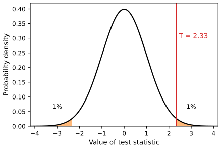
fig_13_1. Reproduces James et al. (2021), Figure 13.1. Download: PDF · SVGpp. 557–558 The p-value is the most used and most abused number in statistics. It is not the probability that \(H_0\) is true; it is the frequency with which data at least as extreme would occur if the experiment were repeated and \(H_0\) held. Its value is that it puts every statistic on one scale: \(T=17.3\) means nothing until we know what \(T\) usually looks like under \(H_0\), and the p-value says exactly that. A two-sided p-value counts both tails; a one-sided p-value needs a scientific reason to look in one direction only. And it is better to report the p-value itself than only whether it crossed 0.05.
Result 13.1 (p-values are uniform under the null) p. 560, "by only rejecting H0 when the p-value is below \(\alpha\), we ensure that the Type I error rate will be less than or equal to \(\alpha\)"
If \(H_0\) holds and the null distribution of \(T\) is continuous, the p-value \(P\) is uniformly distributed on \([0,1]\): \(\Pr_{H_0}(P\le\alpha)=\alpha\) for every \(\alpha\in[0,1]\). If the null distribution is discrete, \(P\) is super-uniform: \(\Pr_{H_0}(P\le\alpha)\le\alpha\). Either way, the test "reject when \(p\le\alpha\)" has Type I error rate at most \(\alpha\).
Filling the gap 13.2: why a p-value is uniform under the null p. 560
Proof
Continuous case. Let \(G(t)=\Pr_{H_0}(|T|\ge t)\), the null tail function of \(|T|\); it is continuous and non-increasing, and \(P=G(|T|)\). Let \(F=1-G\) be the null distribution function of \(|T|\), continuous. The probability integral transform says that \(F(X)\) is uniform when \(X\) has a continuous distribution function \(F\): for \(u\in(0,1)\), let \(x_u=\inf\{x:F(x)\ge u\}\); by continuity \(F(x_u)=u\), and \(F(X)\ge u\) if and only if \(X\ge x_u\) (up to an event of probability zero), so \(\Pr(F(X)\ge u)=\Pr(X\ge x_u)=1-F(x_u)=1-u\). Hence \(F(|T|)\) is uniform, and so is \(P=1-F(|T|)\).
Discrete case. For any \(\alpha\), let \(t_\alpha\) be the smallest attainable value of \(|T|\) with \(G(t_\alpha)\le\alpha\). Then \(P\le\alpha\) exactly when \(|T|\ge t_\alpha\), which has probability \(G(t_\alpha)\le\alpha\). The inequality is strict unless \(\alpha\) is one of the attainable tail probabilities. Example: for ten tosses of a fair coin and the two-sided exact binomial test, \(\Pr(P\le0.05)=0.021\).
The decision rule. The Type I error of "reject when \(P\le\alpha\)" is \(\Pr_{H_0}(P\le\alpha)\), which is \(\alpha\) or less. Confirmed numerically: over 20,000 simulated one-sample t-tests of a true null the p-values pass a Kolmogorov–Smirnov test of uniformity and 5.0% of them fall below 0.05. The full treatment, with pictures, is Filling the gap 6.2 of Statistical Methods for Modern Biology. ∎
Why this matters for the whole chapter. Every multiple-testing procedure below uses only this property of the null p-values. And it explains the problem: among \(m_0\) true nulls, the expected number of p-values below \(\alpha\) is exactly \(m_0\alpha\).
13.1.2 Type I and Type II Errors
Definition 13.2 (errors and power) pp. 559–560, Table 13.1
| \(H_0\) true | \(H_0\) false (\(H_a\) true) | |
|---|---|---|
| reject \(H_0\) | Type I error (false positive) | correct (true positive) |
| do not reject | correct (true negative) | Type II error (false negative) |
The Type I error rate is \(\Pr(\text{reject}\given H_0)\); the power is \(\Pr(\text{reject}\given H_a)=1-\Pr(\text{Type II error})\). The table is the confusion matrix of a classifier whose "positive" is a rejection (Section 4.4.2): the Type I error rate is the false positive rate, the power the sensitivity.
p. 560 The two errors trade off: demanding stronger evidence (smaller \(\alpha\)) makes Type I errors rarer and Type II errors commoner. Because a Type I error announces a finding that is not there, it is usually treated as the more serious, so one fixes \(\alpha\) and then makes the power as large as possible.
Filling the gap 13.3: the trade-off in a formula p. 560
Derivation
Take a statistic \(Z\sim N(\delta,1)\), with \(\delta=0\) under \(H_0\) and \(\delta\ne0\) under the alternative (for a t-test with large samples, \(\delta\) is the true difference in units of its standard error). The two-sided test at level \(\alpha\) rejects when \(|Z|\gt z_{\alpha/2}=\Phi^{-1}(1-\alpha/2)\), and its power is
\[ \beta(\alpha,\delta)=\Pr(|Z|\gt z_{\alpha/2})=\Phi(\delta-z_{\alpha/2})+\Phi(-\delta-z_{\alpha/2}). \]As \(\alpha\) decreases, \(z_{\alpha/2}\) increases and the power decreases: at \(\delta=3\), it is 0.85 for \(\alpha=0.05\), 0.66 for \(\alpha=0.01\), 0.39 for \(\alpha=0.001\) and 0.19 for \(\alpha=10^{-4}\). This formula is behind Figure 13.5: correcting for \(m\) tests lowers the level of each test, and the power follows. Power and sample size for the coin-tossing test are worked out in Filling the gap 6.4 of Statistical Methods for Modern Biology. ∎
13.2 The Challenge of Multiple Testing
pp. 560–561 The book's parable: a stockbroker sends each of 1,024 prospective clients a different one of the \(2^{10}=1{,}024\) possible up/down sequences for a stock over ten days. One client receives the correct sequence and is impressed by a perfect record that was guaranteed to exist. The statistical version: toss 1,024 fair coins ten times each. A single coin with ten tails has a two-sided p-value of \(2/1024\lt 0.002\), yet on average one of the 1,024 coins does it. Make enough guesses and some will be right.
Filling the gap 13.4: how many coins come up all tails? p. 561 and footnote 12
Derivation
Each coin shows ten tails with probability \(2^{-10}=1/1024\), independently, so the number \(N\) of such coins is Binomial\((1024,1/1024)\): \(\E N=1\), and \(\Pr(N\ge1)=1-(1-1/1024)^{1024}=0.632\), close to \(1-e^{-1}\) (the Poisson limit). So in almost two thirds of such experiments at least one coin "looks unfair" at the 0.002 level. The general statement: with \(m\) true null hypotheses each tested at level \(\alpha\), the number of rejections \(V\) has mean \(m\alpha\) (by Result 13.1 and linearity of expectation, whatever the dependence); with \(m=10{,}000\) and \(\alpha=0.01\) that is 100 false rejections. ∎
See also: the same phenomenon, created deliberately by testing repeatedly or choosing the best of several statistics, in p-value hacking (Statistical Methods for Modern Biology, Section 6.6) and its demonstration.
13.3 The Family-Wise Error Rate
13.3.1 What is the Family-Wise Error Rate?
Definition 13.3 (the outcomes of \(m\) tests, and the FWER) p. 562, Table 13.2, (13.3)
| \(H_0\) true | \(H_0\) false | total | |
|---|---|---|---|
| reject | \(V\) | \(S\) | \(R\) |
| do not reject | \(U\) | \(W\) | \(m-R\) |
| total | \(m_0\) | \(m-m_0\) | \(m\) |
\(V\) counts false positives (Type I errors, false discoveries), \(S\) true positives, \(U\) true negatives and \(W\) false negatives (Type II errors). Only \(R\) and \(m-R\) are observed. The family-wise error rate is
\[ \FWER=\Pr(V\ge1). \tag{13.3} \]Result 13.2 (the FWER of uncorrected tests) pp. 562–563, (13.4)–(13.5); Exercise 13.1
Reject every \(H_{0j}\) with \(p_j\le\alpha\). If the \(m_0\) true-null p-values are independent and uniform, then
\[ \FWER(\alpha)=1-\Pr\Big(\bigcap_{j\in\mathcal H_0}\{p_j\gt \alpha\}\Big)=1-(1-\alpha)^{m_0}, \tag{13.4} \]which is the book's \(1-(1-\alpha)^m\) (13.5) when all \(m\) nulls are true. Under arbitrary dependence, \(\alpha\le\FWER(\alpha)\le\min(1,m_0\alpha)\), and both ends are attained.
Filling the gap 13.5: the FWER with and without independence pp. 562–563; Exercise 13.1(c)–(d)
Derivation
Independence. \(V=0\) means that every true null survives; the events \(\{p_j\gt \alpha\}\), \(j\in\mathcal H_0\), are independent with probability \(1-\alpha\) each (Result 13.1), so their intersection has probability \((1-\alpha)^{m_0}\). With \(\alpha=0.05\) and \(m=100\), \(\FWER=1-0.95^{100}=0.994\). Since \((1-\alpha)^m\approx e^{-m\alpha}\), the FWER is close to \(1-e^{-m\alpha}\), which is about \(m\alpha\) when \(m\alpha\) is small.
The book's reading of Figure 13.2 checks out: with \(\alpha=0.01\), \(1-0.99^5=0.049\) but \(1-0.99^6=0.059\), so at most five tests keep the FWER below 0.05; with \(\alpha=0.001\) and \(m=50\), \(1-0.999^{50}=0.0488\).
Lower bound, attained by perfect positive dependence. \(V\ge1\) contains the event that any single true null is rejected, of probability \(\alpha\). If all the null p-values are equal (the same test repeated), \(V\ge1\) is exactly that event and \(\FWER=\alpha\).
Upper bound, attained by perfect negative dependence. \(\Pr(\bigcup_jA_j)\le\sum_j\Pr(A_j)=m_0\alpha\) (the union bound, Result 13.3). Equality holds when the rejection events are disjoint, for example \(m_0=2\) with \(p_2=1-p_1\) and \(\alpha\le0.5\): at most one of the two can be below \(\alpha\), and \(\FWER=2\alpha\). Positive dependence therefore pushes the FWER below \(1-(1-\alpha)^{m_0}\), negative dependence above it; this is Exercise 13.1.
Šidák's level. Testing each hypothesis at \(\alpha_S=1-(1-\alpha)^{1/m}\) gives \(\FWER=\alpha\) exactly for independent tests, a hair less strict than Bonferroni's \(\alpha/m\) (for \(m=10\), \(\alpha=0.05\): 0.005116 against 0.005). Confirmed numerically: 20,000 simulated families of 20 independent tests give an FWER of 0.635 against \(1-0.95^{20}=0.642\). ∎
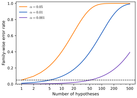
fig_13_2. Reproduces James et al. (2021), Figure 13.2. Download: PDF · SVGp. 563 Back to the single t-test of Section 13.1.1, where the cut-off \(|T|\ge2.33\) gave a Type I error of 0.02. To keep the FWER of ten such tests at 0.02, Section 13.3.2 will test each at 0.002, which moves the cut-off to \(|T|\ge3.09\) (\(=\Phi^{-1}(0.999)\)): controlling the FWER raises the bar for every single hypothesis.
13.3.2 Approaches to Control the Family-Wise Error Rate
p. 564 The examples use the Fund data: monthly percentage excess returns (return above the market) of 2,000 hedge fund managers over \(n=50\) months. For manager \(j\), \(H_{0j}:\mu_j=0\) (no skill) is tested by the one-sample t-statistic \(\sqrt n\,\bar x_j/s_j\) with \(n-1=49\) degrees of freedom.
| manager | mean \(\bar x\) | standard deviation \(s\) | t-statistic | p-value |
|---|---|---|---|---|
| One | 3.0 | 7.42 | 2.86 | 0.0062 |
| Two | −0.1 | 6.86 | −0.10 | 0.9183 |
| Three | 2.8 | 7.55 | 2.62 | 0.0116 |
| Four | 0.5 | 6.71 | 0.53 | 0.6005 |
| Five | 0.3 | 6.78 | 0.31 | 0.7558 |
Table 13.3, recomputed from the Fund data (fund_table in the code); it agrees with the book's table to the digits printed there.
pp. 564–565 Two methods work for any p-values whatever: Bonferroni and Holm. Two others, Tukey's and Scheffé's, are tailored to particular families of tests and are more powerful there.
Result 13.3 (the Bonferroni method) pp. 564–565, (13.6); Exercise 13.3
Reject \(H_{0j}\) when \(p_j\le\alpha/m\). Then \(\FWER\le m_0\alpha/m\le\alpha\), for any dependence between the tests. More generally, testing \(H_{0j}\) at level \(\alpha_j\) gives \(\FWER\le\sum_j\alpha_j\).
Proof
Let \(A_j=\{p_j\le\alpha_j\}\). The union bound \(\Pr(A\cup B)=\Pr(A)+\Pr(B)-\Pr(A\cap B)\le\Pr(A)+\Pr(B)\), applied repeatedly (induction on the number of events), gives \(\Pr(\bigcup_jA_j)\le\sum_j\Pr(A_j)\). Hence
\[ \FWER=\Pr\Big(\bigcup_{j\in\mathcal H_0}A_j\Big)\le\sum_{j\in\mathcal H_0}\Pr(A_j)\le\sum_{j\in\mathcal H_0}\alpha_j, \tag{13.6} \]using \(\Pr(A_j)\le\alpha_j\) for true nulls (Result 13.1); no independence was used. With \(\alpha_j=\alpha/m\) the sum is \(m_0\alpha/m\). ∎
p. 565 On the five managers at \(\alpha=0.05\): without correction Managers One and Three are rejected; Bonferroni tests each at 0.01 and rejects only Manager One. The method is simple and needs no assumptions, which is why it is the best-known correction; its weakness is that it is conservative: the true FWER can be well below \(\alpha\), which costs power. For independent tests of true nulls the loss is small (\(1-(1-\alpha/m)^m\to1-e^{-\alpha}=0.0488\) for \(\alpha=0.05\)); for strongly positively correlated tests it is large.
Deeper: Statistical Learning: Theory and Methods, Section 18.7 (feature assessment and the multiple-testing problem; Bonferroni is Result 18.11).
Algorithm 13.1 (Holm's step-down procedure) p. 566, (13.7)
- Choose \(\alpha\) and compute the p-values \(p_1,\dots,p_m\).
- Sort them, \(p_{(1)}\le\dots\le p_{(m)}\).
- Find the first failure, \(L=\min\{j:p_{(j)}\gt \alpha/(m+1-j)\}\). \(\tag{13.7}\)
- Reject the hypotheses with the \(L-1\) smallest p-values, \(H_{(1)},\dots,H_{(L-1)}\) (all of them if there is no failure).
The smallest p-value faces Bonferroni's threshold \(\alpha/m\); each further one faces a slightly easier threshold \(\alpha/(m-1)\), \(\alpha/(m-2)\), ..., but the procedure stops at the first p-value that fails.
Result 13.4 (Holm controls the FWER) pp. 565–566, "the proof ... is similar to, but slightly more complicated than" (13.6)
For any dependence between the tests, Holm's procedure has \(\FWER\le\alpha\). It rejects every hypothesis that Bonferroni rejects, and possibly more.
Filling the gap 13.6: the proof of Holm's FWER control, and adjusted p-values p. 566; R lab p. 584, "adjusted p-values"
Proof
FWER. Suppose \(m_0\ge1\) (otherwise there is nothing to prove) and let \(p^\star=\min_{j\in\mathcal H_0}p_j\) be the smallest true-null p-value. Consider the event \(B=\{p^\star\gt \alpha/m_0\}\). By the union bound, \(\Pr(B^c)=\Pr\big(\bigcup_{j\in\mathcal H_0}\{p_j\le\alpha/m_0\}\big)\le m_0\cdot\alpha/m_0=\alpha\). We show that on \(B\) Holm makes no false rejection, so \(\FWER\le\Pr(B^c)\le\alpha\).
On \(B\), look at the rank \(k\) of \(p^\star\) among all \(m\) sorted p-values. At most \(m-m_0\) p-values (the false nulls) can be smaller than \(p^\star\), so \(k\le m-m_0+1\), that is \(m+1-k\ge m_0\), and the threshold Holm uses at step \(k\) is \(\alpha/(m+1-k)\le\alpha/m_0\lt p^\star=p_{(k)}\). So step \(k\) fails, \(L\le k\), and Holm stops before reaching \(p^\star\). Every true null has a p-value at least \(p^\star\), so none is rejected. ∎
Holm contains Bonferroni. If \(p_j\le\alpha/m\), every \(p_{(i)}\le p_j\) also satisfies \(p_{(i)}\le\alpha/m\le\alpha/(m+1-i)\), so no failure occurs before \(p_j\) is reached, and \(H_{0j}\) is rejected by Holm too.
Adjusted p-values. R's p.adjust() and Python's multipletests() report, for each hypothesis, the smallest \(\alpha\) at which the procedure would reject it, so that "adjusted \(p\le\alpha\)" is the decision. For Bonferroni this is \(\min(1,mp_j)\). For Holm, \(H_{(j)}\) is rejected at level \(\alpha\) when \((m+1-i)p_{(i)}\le\alpha\) for every \(i\le j\), so its adjusted p-value is the running maximum
For the five managers: \(5\times0.0062=0.0310\) and \(\max(0.0310,4\times0.0116)=0.0464\), both below 0.05, so Holm rejects Managers One and Three, exactly the R lab's output (Section 13.6.2). Confirmed numerically over simulated families of ten tests with five strong effects and correlations 0, 0.5 and \(-0.1\): Holm's FWER is 0.051, 0.043 and 0.050, within Monte Carlo error of the bound. ∎
p. 566 On the five managers at 0.05, the sorted p-values are 0.0062, 0.0116, 0.6005, 0.7558, 0.9183, with Holm thresholds 0.01, 0.0125, 0.0167, 0.025, 0.05. The first two pass and the third fails, so \(L=3\) and Holm rejects Managers One and Three, one more than Bonferroni. (The R edition prints the third threshold as 0.167; it is \(0.05/3=0.0167\), see Notes on the book, 1.)
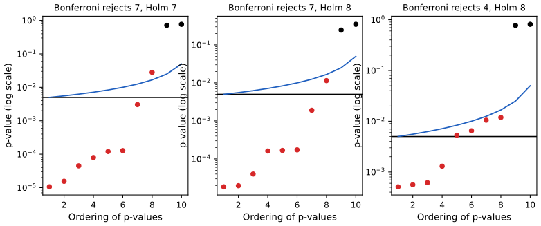
fig_13_3, holm. Reproduces James et al. (2021), Figure 13.3. Download: PDF · SVGpp. 567–569 Tukey's method. Managers One and Two have the largest and smallest means in Table 13.3. Testing \(\mu_1=\mu_2\) only because the table made them stand out is, implicitly, choosing the most extreme of the \(\binom52=10\) pairwise comparisons, so a correction for 10 tests is needed. Bonferroni at 0.005 is valid but too strict, because the ten comparisons are strongly dependent (if \(\bar x_2\approx\bar x_4\) and \(\bar x_2\approx\bar x_5\) then \(\bar x_4\approx\bar x_5\)). Tukey's method uses the exact distribution of the largest of the pairwise statistics and so allows a per-comparison threshold \(\alpha_T\gt \alpha/m\).
Filling the gap 13.7: where Tukey's threshold comes from pp. 567–568
Derivation
Take \(G\) groups of \(n\) observations, independent normal with common variance \(\sigma^2\), and the pooled within-group variance \(s^2\) on \(\nu=G(n-1)\) degrees of freedom. The pairwise statistics are \(t_{jk}=(\bar x_j-\bar x_k)/(s\sqrt{2/n})\). Under the global null \(\mu_1=\dots=\mu_G\), the largest of them is
\[ \max_{j\lt k}|t_{jk}|=\frac{\max_j\bar x_j-\min_j\bar x_j}{s\sqrt{2/n}}=\frac{Q}{\sqrt2},\qquad Q=\frac{\max_j\bar x_j-\min_j\bar x_j}{s/\sqrt n}, \]and \(Q\) has the studentized range distribution with parameters \(G\) and \(\nu\), which does not depend on \(\sigma\). With \(q_{G,\nu}(\alpha)\) its upper \(\alpha\) quantile, rejecting every pair with \(|t_{jk}|\gt q_{G,\nu}(\alpha)/\sqrt2\) gives at least one false rejection, under the global null, with probability exactly \(\alpha\). (Under partial nulls the FWER is at most \(\alpha\) as well, since the range of a subset of means is at most the range of all.) In p-value terms, \(\alpha_T=2\Pr\big(t_\nu\gt q_{G,\nu}(\alpha)/\sqrt2\big)\). The simultaneous intervals \(\bar x_j-\bar x_k\pm q_{G,\nu}(\alpha)\,s/\sqrt n\) are R's TukeyHSD() output.
The numbers. For the five managers (\(G=5\), \(\nu=245\)), \(\alpha_T=0.0064\) against Bonferroni's 0.005. For the setting of Figure 13.4 (\(G=6\), \(n=10\), \(\nu=54\)), \(\alpha_T=0.0046\) against \(0.05/15=0.0033\). Confirmed numerically: 6,000 simulated data sets under the global null give an FWER of 0.044 with \(\alpha_T\) (Monte Carlo standard error 0.003). ∎
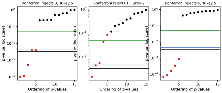
fig_13_4, tukey_alpha. Reproduces James et al. (2021), Figure 13.4. Download: PDF · SVGpp. 568–569 Scheffé's method. Table 13.3 also suggests comparing the two good managers with the three others,
\[ H_0:\ \tfrac12(\mu_1+\mu_3)=\tfrac13(\mu_2+\mu_4+\mu_5), \tag{13.8} \]whose t-test gives \(p=0.004\). Again the hypothesis was chosen after looking, this time among infinitely many possible contrasts. Scheffé's method gives one threshold \(\alpha_S\) that is valid simultaneously for every contrast, so any number of them can be tested after looking at the data. For the Fund managers \(\alpha_S=0.002\), so (13.8) is not rejected.
Filling the gap 13.8: Scheffé's threshold, and the book's numbers p. 569, "it turns out that ... we must set \(\alpha_S=0.002\)"
Derivation
The contrast test. A contrast is \(\psi=\sum_gc_g\mu_g\) with \(\sum_gc_g=0\); (13.8) has \(c=(\frac12,-\frac13,\frac12,-\frac13,-\frac13)\). With group sizes \(n_g\) and the pooled variance \(s^2\) on \(\nu=N-G\) degrees of freedom, \(t_c=\sum_gc_g\bar x_g\big/\big(s\sqrt{\sum_gc_g^2/n_g}\big)\sim t_\nu\) under \(H_0:\psi=0\). For (13.8): \(\hat\psi=2.9-0.233=2.667\), \(t=2.92\), \(p=0.0038\), the book's 0.004.
The largest contrast. Write \(a_g=c_g/\sqrt{n_g}\) and \(b_g=\sqrt{n_g}(\bar x_g-\bar x)\), with \(\bar x\) the grand mean; since \(\sum c_g=0\), \(\sum_gc_g\bar x_g=\sum_ga_gb_g\). By the Cauchy–Schwarz inequality,
\[ t_c^2=\frac{(\sum_ga_gb_g)^2}{s^2\sum_ga_g^2}\le\frac{\sum_gb_g^2}{s^2}=\frac{\sum_gn_g(\bar x_g-\bar x)^2}{s^2}=(G-1)\,F, \]where \(F\) is the one-way ANOVA F-statistic, with equality for \(c_g\propto n_g(\bar x_g-\bar x)\). Under the global null \(F\sim F_{G-1,\nu}\), so rejecting every contrast with \(t_c^2\gt (G-1)F_{G-1,\nu}(\alpha)\) makes a false rejection among all contrasts with probability exactly \(\alpha\).
The threshold. For \(G=5\), \(\nu=245\): \(\sqrt{4F_{4,245}(0.05)}=3.104\), and \(\alpha_S=2\Pr(t_{245}\gt 3.11)=0.0021\), the book's 0.002. Since \(p=0.0038\gt 0.0021\), (13.8) is not rejected. Confirmed numerically: for the five managers the maximising contrast gives \(t^2=8.740=4F\) to machine precision. ∎
p. 569 To sum up: Bonferroni and Holm apply everywhere; in special settings (all pairwise comparisons, all contrasts) Tukey and Scheffé achieve the same FWER guarantee with more power.
13.3.3 Trade-Off Between the FWER and Power
pp. 570–571 Power, in the multiple-testing setting, is the share of false nulls rejected, \(S/(m-m_0)\). Figure 13.5 shows it against the FWER for families in which 90% of the nulls are true.
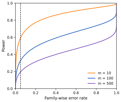
fig_13_5, power_vs_fwer. Reproduces James et al. (2021), Figure 13.5. Download: PDF · SVGThe reason is in the definition: \(\Pr(V\ge1)\le\alpha\) asks for no false positive at all, with high probability, and with many tests the only way to promise that is to reject very little (\(R=0\) guarantees \(V=0\)). For a handful of confirmatory tests this is the right goal; for exploratory screening of thousands of hypotheses, a few false positives are an acceptable price for many more discoveries. That is the idea of the false discovery rate.
13.4 The False Discovery Rate
13.4.1 Intuition for the False Discovery Rate
Definition 13.4 (false discovery proportion and rate) pp. 571–572, (13.9) and footnote 15
The false discovery proportion is \(\FDP=V/R\), set to 0 when \(R=0\); it is a random variable that cannot be observed, since \(V\) is unknown. The false discovery rate is its expectation,
\[ \FDR=\E(\FDP)=\E\Big(\frac{V}{\max(R,1)}\Big)=\E\Big(\frac VR\,\Big|\,R\gt 0\Big)\Pr(R\gt 0). \tag{13.9} \]pp. 571–572 Controlling the FDR at \(q=0.2\) means that, averaged over repetitions of the whole study, at most 20% of the rejections are false; in a given study the share may be higher or lower, just as FWER control at 0.05 does not promise \(V=0\) in any one study. There is no conventional level for \(q\): a researcher who will follow up the discoveries with expensive experiments may choose 10%, one with a cheap follow-up 30%. The motivation is exploratory work, such as testing 20,000 genes for association with a disease, where some false leads are tolerable but 1,000 false leads at the uncorrected 0.05 level (\(0.05\times20{,}000\)) are not.
Filling the gap 13.9: how the FDR compares with the FWER pp. 571–572
Derivation
FDR \(\le\) FWER. Since \(V\le R\), the ratio \(V/\max(R,1)\) is at most 1, and it is 0 when \(V=0\). So \(V/\max(R,1)\le\ind\{V\ge1\}\), and taking expectations, \(\FDR\le\Pr(V\ge1)=\FWER\). Any procedure that controls the FWER at \(\alpha\) controls the FDR at \(\alpha\); the converse fails, which is why FDR control can reject more.
Equality when every null is true. If \(m_0=m\) then \(V=R\), so \(V/\max(R,1)=\ind\{R\ge1\}=\ind\{V\ge1\}\) and \(\FDR=\FWER\). An FDR procedure at level \(q\) therefore also controls the FWER at \(q\) in that case (weak control). Confirmed numerically: with 100 true nulls, Benjamini–Hochberg at \(q=0.1\) rejected something in 10.1% of 6,000 simulated studies. ∎
13.4.2 The Benjamini-Hochberg Procedure
Algorithm 13.2 (Benjamini–Hochberg) p. 573, (13.10)
- Choose \(q\) and compute the p-values \(p_1,\dots,p_m\).
- Sort them, \(p_{(1)}\le\dots\le p_{(m)}\).
- Find the last crossing, \(L=\max\{j:p_{(j)}\le qj/m\}\). \(\tag{13.10}\)
- Reject every \(H_{0j}\) with \(p_j\le p_{(L)}\), that is, the \(L\) smallest; reject nothing if no \(j\) qualifies.
The book writes \(p_{(j)}\lt qj/m\) in (13.10); Benjamini and Hochberg (1995) used \(\le\), as do p.adjust() and multipletests(). The two differ only when a p-value equals its threshold exactly (no difference on the Fund data).
p. 573 On the five managers at \(q=0.05\) the thresholds \(0.05j/5\) are 0.01, 0.02, 0.03, 0.04, 0.05; \(p_{(1)}=0.0062\) and \(p_{(2)}=0.0116\) are below theirs, the other three above, so BH rejects Managers One and Three.
Result 13.5 (Benjamini–Hochberg controls the FDR) p. 573 and footnote 16, "the proof is well beyond the scope of this book"
If the true-null p-values are independent and uniform, and independent of the false-null p-values (whose joint distribution is arbitrary), then the BH procedure at level \(q\) has
\[ \FDR=\frac{m_0}{m}\,q\le q. \]With super-uniform null p-values, \(\FDR\le m_0q/m\). The bound \(\FDR\le q\) also holds under a form of positive dependence (positive regression dependence, PRDS; Benjamini and Yekutieli 2001), which covers one-sided tests of positively correlated normal statistics; under arbitrary dependence it holds after replacing \(q\) by \(q/\sum_{k=1}^m k^{-1}\).
Filling the gap 13.10: a short proof of Result 13.5 p. 573, footnote 16
Proof
Step 1: the FDP as a sum. BH rejects \(H_{0i}\) exactly when \(p_i\le qR/m\), where \(R\) is the number of rejections. Splitting according to the value of \(R\),
\[ \frac{V}{\max(R,1)}=\sum_{i\in\mathcal H_0}\sum_{k=1}^m\frac{\ind\{R=k\}\,\ind\{p_i\le qk/m\}}{k}. \]Step 2: freeze \(p_i\). Let \(R^{(i)}\) be the number of BH rejections when \(p_i\) is replaced by 0; it depends only on the other p-values, hence is independent of \(p_i\) for \(i\in\mathcal H_0\), and \(R^{(i)}\ge1\). The key fact is that, on the event \(\{p_i\le qk/m\}\), \(R=k\) if and only if \(R^{(i)}=k\): whether the last crossing is at \(k\) depends only on the counts of p-values below \(qk'/m\) for \(k'\ge k\), and lowering \(p_i\) to 0 does not change these counts when \(p_i\) is already below \(qk/m\).
Step 3: take expectations. Using that fact, the independence, and \(\Pr(p_i\le qk/m)=qk/m\),
\[ \E\big[\ind\{R=k\}\ind\{p_i\le qk/m\}\big]=\Pr(R^{(i)}=k)\,\frac{qk}{m}, \qquad\text{so}\qquad \FDR=\sum_{i\in\mathcal H_0}\frac qm\sum_{k=1}^m\Pr(R^{(i)}=k)=\frac{m_0}{m}q. \]The inner sum is 1 because \(R^{(i)}\) takes some value in \(\{1,\dots,m\}\). With super-uniform p-values, \(\Pr(p_i\le qk/m)\le qk/m\) and the equalities become \(\le\). The proof of the key fact in Step 2, written out with the counting function \(N(t)=\#\{j:p_j\le t\}\), is in Result 6.6 of Statistical Methods for Modern Biology; the graduate course gives it as Result 18.12. ∎
What the proof does not need. Nothing about the false-null p-values, nor how many nulls are true: the book's "regardless of how many null hypotheses are true, and regardless of the distribution of the p-values for the null hypotheses that are false". Confirmed numerically: 6,000 simulated families with \(m=100\), \(m_0=80\), \(q=0.1\) and independent z-tests give an average FDP of 0.0791 (standard error 0.0009) against the exact \(0.8\times0.1=0.08\).
Filling the gap 13.11: q-values, and BH as an estimated FDR p. 574; R lab p. 586, "the q-values ... can be interpreted as the smallest FDR threshold at which we would reject"
Derivation
BH estimates the FDR of each cut-off. If we reject the \(k\) smallest p-values, i.e. every \(p_j\le p_{(k)}\), the expected number of true nulls among them is at most \(m\,p_{(k)}\) (each of at most \(m\) true-null p-values falls below \(p_{(k)}\) with probability \(p_{(k)}\), if we ignore that \(p_{(k)}\) is itself random). Dividing by the number of rejections \(k\) gives the estimate \(\widehat{\FDR}(k)=m\,p_{(k)}/k\). The BH condition \(p_{(k)}\le qk/m\) is exactly \(\widehat{\FDR}(k)\le q\), and BH takes the largest such \(k\): it rejects as many hypotheses as possible while the estimated FDR stays below \(q\). The estimate is conservative by the factor \(m/m_0\), which is where the \(m_0/m\) of Result 13.5 comes from.
q-values. BH at level \(q\) rejects \(H_{(j)}\) when some \(k\ge j\) has \(m\,p_{(k)}/k\le q\). So the smallest level at which \(H_{(j)}\) is rejected, its BH-adjusted p-value or q-value, is
\[ \tilde q_{(j)}=\min\Big(1,\ \min_{k\ge j}\frac{m\,p_{(k)}}{k}\Big), \]a running minimum from the right. That is why several Fund managers share the q-value 0.07514 in the lab: their own ratios \(mp_{(k)}/k\) are larger, but a later manager with a smaller ratio pulls them all down to it. Step-up versus step-down: Holm stops at the first p-value above its curve; BH looks for the last p-value below its line, so a p-value above the line can still be rejected if a larger one is below it (Figure 13.6, right panel). The same derivation, with the airway data, is Filling the gap 6.13 of Statistical Methods for Modern Biology; the Bayesian reading of the q-value is Filling the gap 18.10 of the graduate course. ∎
pp. 574–575 A fundamental difference from Bonferroni: Bonferroni's threshold \(\alpha/m\) is fixed before seeing the data, while BH's threshold \(p_{(L)}\) depends on all \(m\) p-values. Whether a p-value of 0.01 is rejected at \(q=0.1\) among \(m=100\) tests cannot be known without the other 99 (Holm's threshold is data-dependent too).
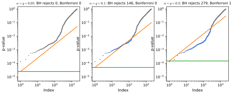
fig_13_6, bh. Reproduces James et al. (2021), Figure 13.6. Download: PDF · SVGDeeper: Statistical Learning: Theory and Methods, Section 18.7.1 (the FDR and BH), and the local false discovery rate in Statistical Methods for Modern Biology, Section 6.10.
p. 575 Many refinements of BH have been proposed since 1995 (estimating \(m_0\), weighting the hypotheses, local FDRs), but the original procedure remains the standard.
13.5 A Re-Sampling Approach to p-Values and False Discovery Rates
pp. 575–576 So far each p-value came from a theoretical null distribution (normal, \(t\), \(\chi^2\), \(F\)), valid under assumptions such as normality or large samples. When the statistic is unusual, or the assumptions are doubtful (small samples, skewed data, outliers), the null distribution can be approximated by computation instead. The book treats the two-sample problem, \(H_0:\E(X)=\E(Y)\) with the statistic
\[ T=\frac{\hat\mu_X-\hat\mu_Y}{s\sqrt{\frac1{n_X}+\frac1{n_Y}}}, \tag{13.11} \]which is (13.1) with \(n_X\) observations of \(X\) and \(n_Y\) of \(Y\).
13.5.1 A Re-Sampling Approach to the p-Value
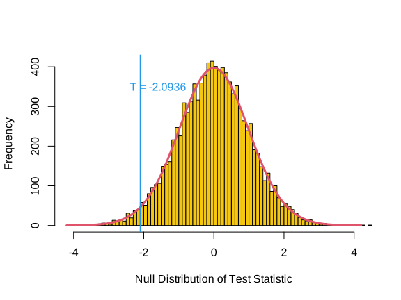
pp. 576–577 The thought experiment: if \(X\) and \(Y\) have the same distribution (a stronger null than equal means), then the group labels carry no information, and swapping observations between the groups does not change the distribution of \(T\). Relabelling at random and recomputing \(T\) many times therefore draws from the null distribution of \(T\).
Algorithm 13.3 (permutation p-value for a two-sample t-test) p. 577, (13.12)
- Compute \(T\) by (13.11) on the data \(x_1,\dots,x_{n_X}\), \(y_1,\dots,y_{n_Y}\).
- For \(b=1,\dots,B\) (e.g. \(B=10{,}000\)): permute the \(n_X+n_Y\) pooled observations at random, call the first \(n_X\) of them \(x^*\) and the rest \(y^*\), and compute \(T^{*b}\) by (13.11).
- Report \[ p=\frac{\sum_{b=1}^B\ind\big(|T^{*b}|\ge|T|\big)}{B}. \tag{13.12} \]
Result 13.6 (permutation p-values are valid) pp. 576–577
Suppose that under \(H_0\) the \(n=n_X+n_Y\) observations are exchangeable (for example, independent and identically distributed). (a) The exact permutation p-value, the share of all \(\binom{n}{n_X}\) relabellings with \(|T^*|\ge|T|\), satisfies \(\Pr_{H_0}(p\le\alpha)\le\alpha\) for every \(\alpha\). (b) With \(B\) random relabellings, \(p^+=\big(1+\sum_b\ind(|T^{*b}|\ge|T|)\big)/(B+1)\) also satisfies \(\Pr_{H_0}(p^+\le\alpha)\le\alpha\); the book's (13.12) differs from it by at most \(1/B\).
Filling the gap 13.12: why relabelling gives a valid p-value, and what it assumes pp. 576–577, footnote 17
Proof
(a) Condition on the unordered set of the \(n\) observed values. Under exchangeability, every assignment of \(n_X\) of them to group \(X\) is equally likely, and the observed assignment is one of them, chosen uniformly. List the values of \(|T|\) over all \(K=\binom n{n_X}\) assignments; the observed \(|T|\) is a uniform draw from this list, and \(p\) is the share of the list at or above it. For a uniform draw from a finite list, the share at or above it is at most \(\alpha\) with probability at most \(\alpha\) (if the observed value is the \(r\)-th largest, \(p\ge r/K\), and at most \(\lfloor\alpha K\rfloor\) values have rank \(r\le\alpha K\)). This holds conditionally on every data set, hence unconditionally. No normality, no large sample, only exchangeability.
(b) Under \(H_0\) the observed labelling and the \(B\) random relabellings are \(B+1\) exchangeable draws, so the rank of \(|T|\) among the \(B+1\) values \(|T|,|T^{*1}|,\dots,|T^{*B}|\) is uniform (ties broken at random, which only helps), and \(p^+\) is that rank divided by \(B+1\). With (13.12), \(p=0\) is possible, which no valid p-value should allow at \(\alpha\lt 1/(B+1)\); in practice the difference matters only for very small p-values (demonstration, preset 4).
What the null hypothesis is. The permutation test tests "same distribution", not "same mean". If the variances differ (and the group sizes differ), the pooled \(T\) can reject equal means too often even under permutation; studentising helps, and Welch's statistic is the usual remedy. The exact case with every relabelling enumerated is Result 6.4 of Statistical Methods for Modern Biology, and Filling the gap 18.8 of the graduate course discusses what permutation p-values assume. ∎
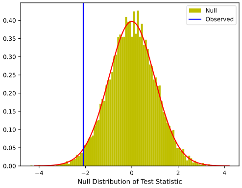
p. 577 The Khan data (ISLR2 package) hold the expression of 2,308 genes for 83 patients with one of four types of small round blue cell tumours of childhood. The book compares its class 2 (29 patients) with class 4 (25 patients); in the original study these sizes are those of Ewing's sarcoma and rhabdomyosarcoma (the book names them differently; Notes on the book, 3). For gene 11, \(T=-2.0936\); the \(t_{52}\) p-value is 0.0412 and the permutation p-value with \(B=10{,}000\) is 0.0396 here (0.042 in the book, 0.0416 in the R lab, 0.0398 in the Python lab: the differences are Monte Carlo error, with standard error \(\sqrt{0.04\times0.96/10^4}=0.002\)).
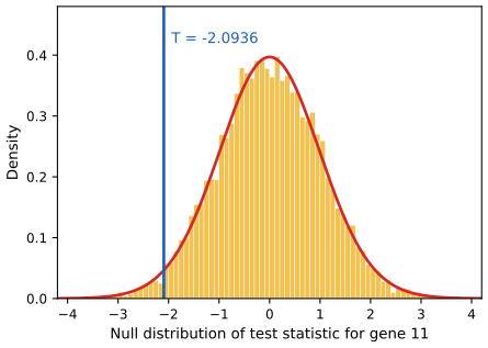
fig_13_7, khan_permutations. Reproduces James et al. (2021), Figure 13.7. Download: PDF · SVG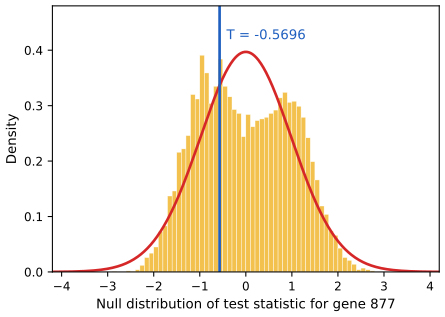
fig_13_8. Reproduces James et al. (2021), Figure 13.8. Download: PDF · SVGFilling the gap 13.13: why one outlier gives gene 877 a two-humped null p. 578, "a single observation in the 877th gene is very far from the other observations"
Explanation
The first patient of class 2 has expression \(-5.38\) for gene 877; the other 53 values have mean 0.39 and standard deviation 0.53, so it lies about 11 standard deviations away. Under relabelling, this value goes to the group of 29 with probability \(29/54=0.54\) and to the group of 25 otherwise, and wherever it goes it dominates: it pulls that group's mean down by about \(5.77/29=0.20\) or \(5.77/25=0.23\) and inflates the pooled standard deviation \(s\) from about 0.53 to about 0.95. So \(T^*\) is centred near \(-0.20/(0.95\times0.27)\approx-0.8\) when the outlier is in the first group and near \(+0.23/(0.95\times0.27)\approx+0.9\) when it is in the second. A simulation of the two cases gives means \(-0.78\) and \(+0.90\), each with standard deviation 0.57: the two humps of Figure 13.8. The \(t_{52}\) distribution assumes normal data, and one value 11 standard deviations out is not compatible with that. Removing the outlier gives \(T=0.35\) and \(p=0.73\). ∎
Deeper: Statistical Learning: Theory and Methods, Section 18.7, Filling the gap 18.8 (permutation p-values for many genes, and what they assume).
13.5.2 A Re-Sampling Approach to the False Discovery Rate
pp. 578–580 For \(m\) hypotheses we could compute \(m\) permutation p-values and apply BH. The book describes a more direct route. Reject every \(H_{0j}\) with \(|T_j|\ge c\); then \(R=\sum_j\ind(|T_j|\ge c)\) is observed and only \(V\) is unknown. Approximate
\[ \FDR=\E\Big(\frac VR\Big)\approx\frac{\E(V)}{R}, \tag{13.13} \]and estimate \(\E(V)\) by the number of statistics beyond \(c\) in data where every null holds by construction: the relabelled data.
Algorithm 13.4 (plug-in FDR for two-sample t-tests) p. 580
- Choose a threshold \(c\gt 0\).
- For each \(j=1,\dots,m\): compute \(T^{(j)}\) on the original data, and \(T^{(j),*b}\) on \(B\) random relabellings, \(b=1,\dots,B\).
- \(R=\sum_j\ind(|T^{(j)}|\ge c)\) and \(\hat V=\frac1B\sum_b\sum_j\ind(|T^{(j),*b}|\ge c)\).
- The estimated FDR of the threshold \(c\) is \(\hat V/R\).
Using the same relabellings for all genes (the book's footnote 18) lets one matrix product compute all \(m\) statistics of a relabelling at once; the code (perm_tstats) does this, and 10,000 relabellings of all 2,308 genes take a few seconds.
p. 580 Define the pooled re-sampling p-value of gene \(j\) by comparing \(|T_j|\) with the relabelled statistics of all genes,
\[ p_j=\frac{\sum_{j'=1}^m\sum_{b=1}^B\ind\big(|T^{*b}_{j'}|\ge|T_j|\big)}{Bm}. \tag{13.14} \]Result 13.7 (BH on the pooled p-values is the plug-in rule) p. 580, "exactly equivalent to Algorithm 13.4"
Let the thresholds run over the observed values, \(c=|T|_{(k)}\), the \(k\)-th largest \(|T_j|\) (no ties). Then \(\hat V/R\) at \(c=|T|_{(k)}\) equals \(m\,p_{(k)}/k\) computed from the pooled p-values (13.14). Hence "reject the \(k\) largest \(|T_j|\) for the largest \(k\) with \(\hat V/R\le q\)" and BH at level \(q\) on the pooled p-values reject the same genes.
Proof
Large \(|T|\) means small pooled p-value, and (13.14) is decreasing in \(|T_j|\), so the gene with the \(k\)-th largest \(|T|\) has the \(k\)-th smallest pooled p-value, \(p_{(k)}=\sum_{j',b}\ind(|T^{*b}_{j'}|\ge|T|_{(k)})/(Bm)=\hat V(|T|_{(k)})/m\). With \(c=|T|_{(k)}\), exactly \(k\) observed statistics reach \(c\), so \(R=k\), and \(\hat V/R=m\,p_{(k)}/k\). The BH condition \(p_{(k)}\le qk/m\) is \(\hat V/R\le q\), and both rules take the largest such \(k\) (Filling the gap 13.11). Confirmed numerically on the Khan data at \(q=0.05\), 0.1, 0.2 and 0.3. The graduate course states it as Result 18.13. ∎
Filling the gap 13.14: what \(\hat V\) estimates, and the approximation (13.13) pp. 578–579
Explanation
The numerator. In relabelled data every gene behaves like a true null, so \(\hat V\) estimates \(m\Pr_0(|T|\ge c)\), the number of rejections we would expect if all \(m\) nulls were true. The actual \(\E(V)\) involves only the \(m_0\) true nulls, \(m_0\Pr_0(|T|\ge c)\). So \(\hat V\) overestimates \(\E(V)\) by the factor \(m/m_0\), and the plug-in FDR is conservative, exactly as BH (Result 13.5). Estimating \(m_0\) and multiplying by \(\hat m_0/m\) gives a sharper estimate; this is part of the SAM procedure (Filling the gap 18.9 and Section 18.7.2 of the graduate course). A second caveat: when the false nulls have large effects, relabelling mixes groups that really differ, which inflates the spread of the relabelled statistics of those genes and makes \(\hat V\) slightly larger still.
The ratio. \(\E(V/R)\approx\E(V)/R\) treats \(R\) as fixed. For a fixed cut-off \(c\) and large \(m\), \(R/m\) concentrates around its mean (a law of large numbers over many weakly dependent genes), and the approximation is good; for few tests it is rough. ∎
Deeper: Statistical Learning: Theory and Methods, Section 18.7.1, Algorithm 18.3 (the plug-in FDR) and Section 18.7.2 (asymmetric cut-points and the SAM procedure).
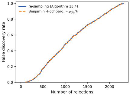
fig_13_9, plugin_fdr. Reproduces James et al. (2021), Figure 13.9. Download: PDF · SVG13.5.3 When Are Re-Sampling Approaches Useful?
pp. 581–582 Two situations call for re-sampling: no theoretical null distribution is available (an unusual hypothesis or statistic), or one is available but its assumptions fail (the \(t_{n_X+n_Y-2}\) null needs normal data; the \(N(0,1)\) approximation needs large samples). Gene 877 shows the second case. The general recipe: find a way to resample or permute the data so that the null holds by construction, and compute p-values or FDRs from the resampled statistics. The book's footnote says that when the two approaches disagree, the re-sampling result is "more trustworthy"; that is right when the exchangeability assumption itself is plausible, which it is not, for instance, when the null of interest allows unequal variances (Filling the gap 13.12).
13.6 Lab: Multiple Testing
The R lab of James et al. (2021) and the Python lab of James et al. (2023) do the same analyses with different random numbers. Below, each step shows my R code (left) and my Python code (right), from ch13_lab.R and ch13_lab.py; lines that only store numbers for later comparison are omitted. The R code uses the same seeds as the R edition and the Python code the same random generator, in the same order, as the Python edition, so each reproduces its own edition's printed output (with two exceptions in the Python edition, Notes on the book, 4 and 5). Everything that does not depend on random numbers agrees between the two languages to at least seven significant digits, except Tukey's adjusted p-values (to about four digits, Section 13.6.2).
R ch13_lab.R
suppressPackageStartupMessages(library(ISLR2))   # Fund, Khan, Carseats
options(digits = 5, width = 100)
Python ch13_lab.py
import numpy as np
import pandas as pd
import statsmodels.api as sm
from scipy.stats import f as f_dbn, studentized_range, t as t_dbn, ttest_1samp, ttest_ind, ttest_rel
from statsmodels.stats.multicomp import pairwise_tukeyhsd
from statsmodels.stats.multitest import multipletests as mult_test

import common
Where the languages differ
- Random numbers. R's
set.seed()/sample()and numpy'sdefault_rng()/shuffle()are different generators, so the simulated data of 13.6.1, the permutations of 13.6.4 and the 100 random genes differ. The R lab therefore reproduces the R edition's numbers and the Python lab the Python edition's; they agree with each other only up to Monte Carlo error. - Khan in Python. Khan exists only in the R package; the Python code reads the copy exported once from R (
khan()in ch13_multiple_testing.py). - Speed. Both labs compute the t-statistic of a relabelling with a short function (R:
tstat; Python:tstat_rows, vectorised over all relabellings) instead of callingt.test()orttest_ind()a million times. This does not change the random numbers drawn, so the results are those of the books' slower code; the whole R lab runs in about 45 seconds, the Python lab in about 15.
13.6.1 Review of Hypothesis Tests
One hundred variables of ten observations each; the first 50 have mean 0.5 (false nulls), the last 50 mean 0. A one-sample t-test of \(\mu_j=0\) for each, and the \(2\times2\) table of decisions against the truth (Table 13.2, transposed).
R ch13_lab.R
# The random draws follow the R lab of the book (set.seed(6), set.seed(1)), so the printed numbers
# can be compared with it. The Python version is ch13_lab.py. Run from the code/ folder:
#   Rscript ch13_lab.R          (about 20 seconds)
# Figures go to ../img/ch13/lab-r-*.svg (and .pdf) and the key numbers to cache/ch13_lab_R.csv.

suppressPackageStartupMessages(library(ISLR2))   # Fund, Khan, Carseats
options(digits = 5, width = 100)

out_dir <- file.path("..", "img", "ch13")
dir.create(out_dir, showWarnings = FALSE, recursive = TRUE)
dir.create("cache", showWarnings = FALSE)
key <- list()                                 # key numbers, written to cache/ch13_lab_R.csv at the end
keep <- function(name, value) key[[name]] <<- unname(as.numeric(value))
save_plot <- function(name, width, height, draw) {   # the same plot as SVG (for the web) and PDF
  if (requireNamespace("svglite", quietly = TRUE)) svglite::svglite(file.path(out_dir, paste0(name, ".svg")), width, height)
  else grDevices::svg(file.path(out_dir, paste0(name, ".svg")), width, height)
  draw(); invisible(dev.off())
  pdf(file.path(out_dir, paste0(name, ".pdf")), width, height); draw(); invisible(dev.off())
}

# ================================================================== 13.6.1 review of hypothesis tests
set.seed(6)
x <- matrix(rnorm(10 * 100), 10, 100)        # 100 variables, 10 observations each
x[, 1:50] <- x[, 1:50] + 0.5                 # the first 50 have mean 0.5: H0 is false for them
tt1 <- t.test(x[, 1], mu = 0)
tt1                                          # t = 2.08, df = 9, p = 0.067: a Type II error

p.values <- apply(x, 2, function(col) t.test(col, mu = 0)$p.value)
decision <- ifelse(p.values <= 0.05, "Reject H0", "Do not reject H0")
truth <- rep(c("H0 is False", "H0 is True"), each = 50)
tab1 <- table(decision, truth)
tab1                                         # W = 40, U = 47, S = 10, V = 3
Python ch13_lab.py
rng = np.random.default_rng(12)
X = rng.standard_normal((10, 100))            # 100 variables, 10 observations each
true_mean = np.array([0.5] * 50 + [0] * 50)
X += true_mean[None, :]
result = ttest_1samp(X[:, 0], 0)
show("first variable: t, p =", (round(result.statistic, 4), round(result.pvalue, 4)))   # p = 0.931

def crosstab(p_values, true_mean):
    decision = pd.Categorical(np.where(p_values <= 0.05, "Reject H0", "Do not reject H0"),
                              categories=["Do not reject H0", "Reject H0"])
    truth = pd.Categorical(np.where(true_mean == 0, "H0 is True", "H0 is False"),
                           categories=["H0 is False", "H0 is True"])
    return pd.crosstab(decision, truth, rownames=["decision"], colnames=["truth"], dropna=False)

p_values = ttest_1samp(X, 0).pvalue           # all 100 tests at once (one per column)
tab1 = crosstab(p_values, true_mean)
print(tab1)                                   # S = 15, V = 5 in this draw
Then the stronger signal, mean 1 for the false nulls:
R ch13_lab.R
x <- matrix(rnorm(10 * 100), 10, 100)        # a stronger signal: mean 1 for the false nulls
x[, 1:50] <- x[, 1:50] + 1
p.values <- apply(x, 2, function(col) t.test(col, mu = 0)$p.value)
decision <- ifelse(p.values <= 0.05, "Reject H0", "Do not reject H0")
tab2 <- table(decision, truth)
tab2                                         # W = 9, U = 49, S = 41, V = 1
Python ch13_lab.py
true_mean = np.array([1] * 50 + [0] * 50)     # a stronger signal
X = rng.standard_normal((10, 100))
X += true_mean[None, :]
p_values = ttest_1samp(X, 0).pvalue
tab2 = crosstab(p_values, true_mean)
print(tab2) # S = 40, V = 2| first test | effect 0.5: \(W\), \(S\), \(U\), \(V\) | effect 1: \(W\), \(S\), \(U\), \(V\) | |||||||
|---|---|---|---|---|---|---|---|---|---|
R, set.seed(6) | \(t=2.08\), \(p=0.067\) | 40 | 10 | 47 | 3 | 9 | 41 | 49 | 1 |
Python, default_rng(12) | \(p=0.931\) | 35 | 15 | 45 | 5 | 10 | 40 | 48 | 2 |
Each row is its own edition's output. In both, the first test misses a real effect (a Type II error), about 5% of the 50 true nulls are rejected (3 and 5), and with effect 0.5 most false nulls are missed (power 0.20 and 0.30; the exact power of a one-sample t-test with \(n=10\) and effect 0.5 is 0.29). Doubling the effect raises the power to about 0.8.
13.6.2 The Family-Wise Error Rate
Formula (13.5) for \(m=1,\dots,500\) and three levels (Figure 13.2):
R ch13_lab.R
m <- 1:500
fwe <- sapply(c(0.05, 0.01, 0.001), function(a) 1 - (1 - a)^m)   # (13.5), one column per alpha
save_plot("lab-r-fwer", 6, 4.5, function() {
  matplot(m, fwe, type = "l", lty = 1, lwd = 2, log = "x", ylim = c(0, 1), col = c(2, 4, 3),
          xlab = "Number of Hypotheses", ylab = "Family-Wise Error Rate")
  abline(h = 0.05, lty = 2)
  legend("topleft", legend = c("alpha = 0.05", "alpha = 0.01", "alpha = 0.001"), col = c(2, 4, 3), lwd = 2, bty = "n")
})
Python ch13_lab.py
m = np.arange(1, 501)
fig, ax = plt.subplots(figsize=(6, 4.5))
for alpha in (0.05, 0.01, 0.001):
    ax.plot(m, 1 - (1 - alpha) ** m, label=r"$\alpha=%s$" % alpha)      # (13.5)
ax.set_xscale("log")
ax.set(xlabel="Number of Hypotheses", ylabel="Family-Wise Error Rate", ylim=(0, 1))
ax.legend()
ax.axhline(0.05, c="k", ls="--")
save(fig, "lab-py-fwer")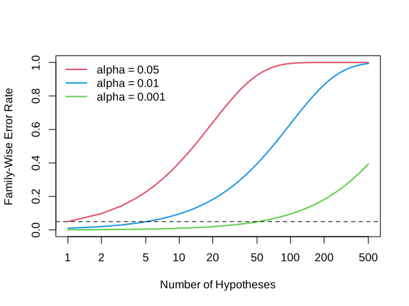
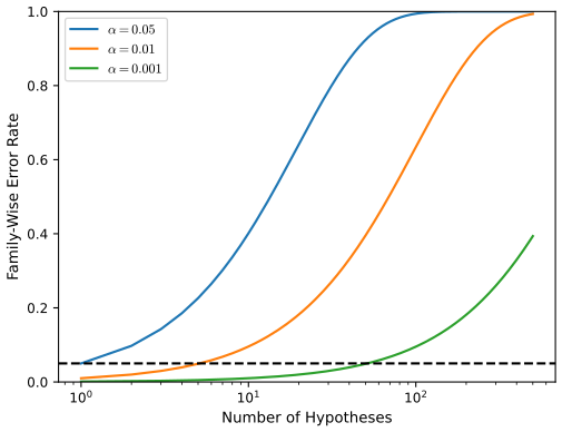
One-sample t-tests for the first five managers, then Bonferroni and Holm, with the adjusted p-values of Filling the gap 13.6 also computed by hand:
R ch13_lab.R
fund.mini <- Fund[, 1:5]
t.test(fund.mini[, 1], mu = 0)               # t = 2.86, p = 0.0062
fund.pvalue <- sapply(fund.mini, function(col) t.test(col, mu = 0)$p.value)
fund.pvalue                                  # 0.0062 0.9183 0.0116 0.6005 0.7558

p_bonf <- p.adjust(fund.pvalue, method = "bonferroni")
p_bonf                                       # only Manager One is below 0.05
all.equal(p_bonf, pmin(fund.pvalue * 5, 1))  # Bonferroni: multiply by m, cap at 1
p_holm <- p.adjust(fund.pvalue, method = "holm")
p_holm                                       # Managers One and Three are below 0.05

# Holm's adjusted p-values by hand: sort, multiply the j-th smallest by m + 1 - j,
# take the running maximum, cap at 1, and put back in the original order.
holm_by_hand <- function(p) {
  m <- length(p); o <- order(p)
  adj <- pmin(1, cummax((m + 1 - seq_len(m)) * p[o]))
  adj[order(o)]
}
all.equal(unname(holm_by_hand(fund.pvalue)), unname(p_holm))   # TRUE
Python ch13_lab.py
Fund = common.isl_data("Fund", index_col=0)  # 50 months x 2,000 managers
fund_mini = Fund.iloc[:, :5]
res = ttest_1samp(fund_mini, 0)               # one test per column
fund_mini_pvals = res.pvalue
show("five managers, p-values:", np.round(fund_mini_pvals, 4))           # 0.0062 0.9183 0.0116 0.6005 0.7558

reject, bonf = mult_test(fund_mini_pvals, method="bonferroni")[:2]
show("Bonferroni:", (reject, np.round(bonf, 4)))                       # only Manager One
show("  = min(5 p, 1):", np.allclose(bonf, np.minimum(fund_mini_pvals * 5, 1)))
reject, holm = mult_test(fund_mini_pvals, method="holm", alpha=0.05)[:2]
show("Holm:", (reject, np.round(holm, 4)))                             # Managers One and Three

# Holm's adjusted p-values by hand: the j-th smallest times m + 1 - j, running maximum, cap at 1.
def holm_by_hand(p):
    m = len(p)
    o = np.argsort(p)
    adj = np.minimum(1, np.maximum.accumulate((m - np.arange(m)) * p[o]))
    out = np.empty(m)
    out[o] = adj
    return out

show(" Holm by hand agrees:", np.allclose(holm_by_hand(fund_mini_pvals), holm))| manager | 1 | 2 | 3 | 4 | 5 |
|---|---|---|---|---|---|
| p-value | 0.0062 | 0.9183 | 0.0116 | 0.6005 | 0.7558 |
| Bonferroni adjusted | 0.0310 | 1 | 0.0580 | 1 | 1 |
| Holm adjusted | 0.0310 | 1 | 0.0464 | 1 | 1 |
Identical in R and Python. At FWER 0.05, Bonferroni rejects Manager One, Holm Managers One and Three.
Managers One and Two have the highest and lowest means. A paired t-test (the months are the same for both managers) gives \(p=0.038\); but the pair was chosen after looking at all ten pairs, so Tukey's method is applied to the one-way ANOVA of the 250 returns:
R ch13_lab.R
colMeans(fund.mini)                          # 3.0 -0.1 2.8 0.5 0.3
tt_pair <- t.test(fund.mini[, 1], fund.mini[, 2], paired = TRUE)
tt_pair                                      # t = 2.13, p = 0.038
tt_two <- t.test(fund.mini[, 1], fund.mini[, 2], var.equal = TRUE)
tt_two$p.value                               # the unpaired two-sample test (13.1): 0.0349

returns <- as.vector(as.matrix(fund.mini))   # one long vector, manager by manager
manager <- factor(rep(1:5, each = 50))
a1 <- aov(returns ~ manager)
tukey <- TukeyHSD(x = a1)
tukey                                        # 2-1: diff -3.1, p adj 0.1862
save_plot("lab-r-tukey", 6, 5, function() { par(las = 1); plot(tukey) })
Python ch13_lab.py
show("means:", fund_mini.mean().to_numpy())                               # 3.0 -0.1 2.8 0.5 0.3
pair_p = ttest_rel(fund_mini["Manager1"], fund_mini["Manager2"]).pvalue
two_p = ttest_ind(fund_mini["Manager1"], fund_mini["Manager2"], equal_var=True).pvalue
show("paired t-test p:", round(pair_p, 4))                                 # 0.038
show("unpaired two-sample t-test p:", round(two_p, 4))                     # 0.0324

returns = np.hstack([fund_mini.iloc[:, i] for i in range(5)])
managers = np.hstack([[i + 1] * 50 for i in range(5)])
tukey = pairwise_tukeyhsd(returns, managers)
print(tukey.summary())                        # 1-2: meandiff -3.1, p-adj 0.1862
fig, ax = plt.subplots(figsize=(6, 5))
tukey.plot_simultaneous(ax=ax)
save(fig, "lab-py-tukey")| pair | 2−1 | 3−1 | 4−1 | 5−1 | 3−2 | 4−2 | 5−2 | 4−3 | 5−3 | 5−4 |
|---|---|---|---|---|---|---|---|---|---|---|
| difference | −3.1 | −0.2 | −2.5 | −2.7 | 2.9 | 0.6 | 0.4 | −2.3 | −2.5 | −0.2 |
| Tukey adjusted p | 0.1862 | 0.9999 | 0.3948 | 0.3152 | 0.2453 | 0.9932 | 0.9986 | 0.4820 | 0.3948 | 0.9999 |
All intervals have half-width 3.8865 (equal group sizes) and contain 0: after adjusting for the ten comparisons, the p-value for Managers One and Two rises from 0.038 to 0.186. R's TukeyHSD() and Python's pairwise_tukeyhsd() agree to the four digits printed (they use different numerical routines for the studentized range distribution; the adjusted p-values agree to within \(2\times10^{-4}\)). Python labels the pairs "1 2" with the difference \(\bar x_2-\bar x_1\), as R does.
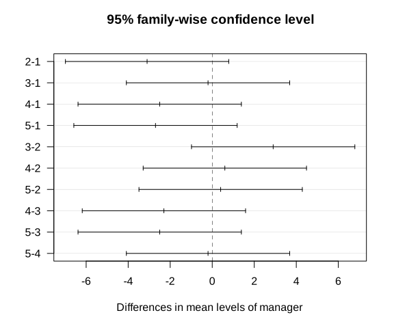
plot(TukeyHSD(a1)), the ten simultaneous intervals for the differences; all contain 0. PDF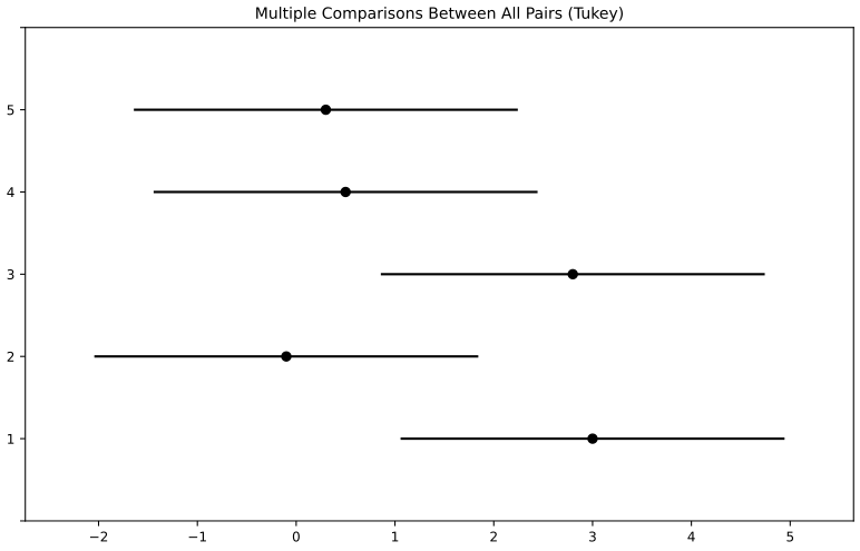
plot_simultaneous(), one interval per manager; two managers differ significantly when their intervals do not overlap (none here). PDFBeyond the book's lab, Tukey's per-comparison threshold and Scheffé's test of the contrast (13.8) (Filling the gaps 13.7 and 13.8):
R ch13_lab.R
# Beyond the book's lab: the p-value threshold of Tukey's method for these ten comparisons,
# and Scheffe's test of the contrast (13.8), managers 1 and 3 against 2, 4 and 5.
df_res <- df.residual(a1)                    # 250 - 5 = 245
s2 <- sum(residuals(a1)^2) / df_res          # pooled within-manager variance
alpha_T <- 2 * pt(qtukey(0.95, 5, df_res) / sqrt(2), df_res, lower.tail = FALSE)
cvec <- c(1/2, -1/3, 1/2, -1/3, -1/3)
est <- sum(cvec * colMeans(fund.mini))
t_contrast <- est / sqrt(s2 * sum(cvec^2) / 50)
p_contrast <- 2 * pt(abs(t_contrast), df_res, lower.tail = FALSE)
crit_S <- sqrt(4 * qf(0.95, 4, df_res))      # Scheffe: reject if |t| > sqrt((G - 1) F)
alpha_S <- 2 * pt(crit_S, df_res, lower.tail = FALSE)
c(alpha_T = alpha_T, t = t_contrast, p = p_contrast, alpha_S = alpha_S)   # p = 0.004, alpha_S = 0.002
Python ch13_lab.py
# Beyond the book's lab: Tukey's p-value threshold, and Scheffe's test of the contrast (13.8).
df_res = len(returns) - 5
s2 = sum(((fund_mini.iloc[:, g] - fund_mini.iloc[:, g].mean()) ** 2).sum() for g in range(5)) / df_res
alpha_T = 2 * t_dbn.sf(studentized_range.ppf(0.95, 5, df_res) / np.sqrt(2), df_res)
c = np.array([1 / 2, -1 / 3, 1 / 2, -1 / 3, -1 / 3])
est = c @ fund_mini.mean().to_numpy()
t_contrast = est / np.sqrt(s2 * np.sum(c ** 2) / 50)
p_contrast = 2 * t_dbn.sf(abs(t_contrast), df_res)
alpha_S = 2 * t_dbn.sf(np.sqrt(4 * f_dbn.ppf(0.95, 4, df_res)), df_res)
show("alpha_T, contrast t and p, alpha_S:", np.round([alpha_T, t_contrast, p_contrast, alpha_S], 5))
Both give \(\alpha_T=0.00644\), \(t=2.921\), \(p=0.00381\) and \(\alpha_S=0.00213\): the contrast (13.8) is not significant once the data-driven choice is accounted for. The unpaired pooled t-test of Managers One and Two gives \(p=0.0324\) (both languages); the book's 0.0349 is discussed in Notes on the book, 2.
13.6.3 The False Discovery Rate
A one-sample t-test for each of the 2,000 managers, BH q-values, and the comparison with Bonferroni:
R ch13_lab.R
fund.pvalues <- sapply(Fund, function(col) t.test(col, mu = 0)$p.value)   # 2,000 one-sample tests
q.values.BH <- p.adjust(fund.pvalues, method = "BH")
q.values.BH[1:10]                            # 0.0899 0.9915 0.1221 0.9234 0.9560 0.0751 ...
sum(q.values.BH <= 0.1)                      # 146 managers at an FDR of 10%
sum(fund.pvalues <= 0.1 / 2000)              # Bonferroni at 0.1 rejects none
Python ch13_lab.py
fund_pvalues = ttest_1samp(Fund, 0).pvalue    # 2,000 one-sample tests
fund_qvalues = mult_test(fund_pvalues, method="fdr_bh")[1]
show("first ten q-values:", np.round(fund_qvalues[:10], 4))
show("q <= 0.1:", (fund_qvalues <= 0.1).sum())                             # 146
show("Bonferroni at 0.1:", (fund_pvalues <= 0.1 / 2000).sum()) # 0| manager | 1 | 2 | 3 | 4 | 5 | 6 | 7 | 8 | 9 | 10 |
|---|---|---|---|---|---|---|---|---|---|---|
| BH q-value | 0.0899 | 0.9915 | 0.1221 | 0.9234 | 0.9560 | 0.0751 | 0.0767 | 0.0751 | 0.0751 | 0.0751 |
The same in both languages and in both editions: 146 managers have a q-value at most 0.1, and Bonferroni at 0.1 rejects none. Then BH by hand, Algorithm 13.2, and the centre panel of Figure 13.6:
R ch13_lab.R
# Benjamini-Hochberg by hand (Algorithm 13.2): the largest j with p_(j) <= q j / m,
# then reject the j smallest p-values.
ps <- sort(fund.pvalues)
m <- length(fund.pvalues)
q <- 0.1
wh.ps <- which(ps <= q * (1:m) / m)
wh <- if (length(wh.ps) > 0) 1:max(wh.ps) else integer(0)
length(wh)                                   # 146 again
save_plot("lab-r-bh", 6, 4.5, function() {
  plot(ps, log = "xy", ylim = c(4e-6, 1), xlab = "Index", ylab = "P-Value", pch = 20, cex = 0.5, col = "grey40")
  points(wh, ps[wh], col = 4, pch = 20, cex = 0.6)
  abline(a = 0, b = q / m, col = 2, untf = TRUE)  # untf = TRUE draws the straight line p = qj/m on log axes
  abline(h = 0.1 / 2000, col = 3)
})
Python ch13_lab.py
# Benjamini-Hochberg by hand (Algorithm 13.2)
sorted_ = np.sort(fund_pvalues)
m = fund_pvalues.shape[0]
q = 0.1
passing = np.nonzero(sorted_ <= q * np.arange(1, m + 1) / m)[0]
L = passing.max() + 1 if len(passing) else 0          # number of rejections
selected_ = fund_pvalues <= sorted_[L - 1] if L else np.zeros(m, bool)
show("BH by hand:", (L, selected_.sum()))                                  # 146 146
fig, ax = plt.subplots(figsize=(6, 4.5))
j = np.arange(1, m + 1)
ax.scatter(j, sorted_, s=6, c="grey")
ax.scatter(j[:L], sorted_[:L], s=8, c="b")
ax.plot(j, q * j / m, c="r")                  # the line p = q j / m, drawn point by point
ax.axhline(q / m, c="g")
ax.set(xscale="log", yscale="log", xlabel="Index", ylabel="P-Value", ylim=(4e-6, 1.2))
save(fig, "lab-py-bh")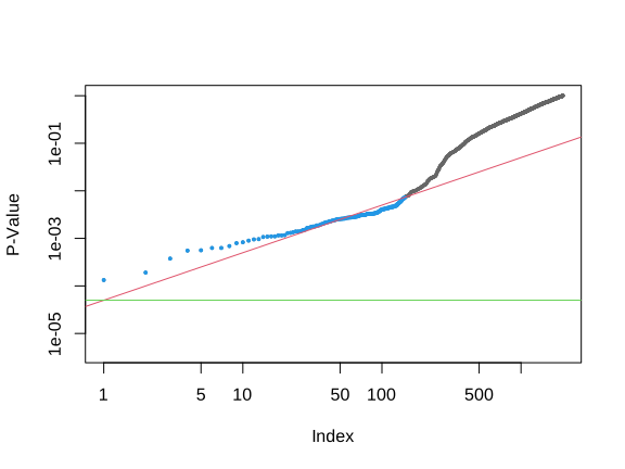
abline(..., untf = TRUE) draws the line \(p=qj/m\) correctly on log axes. PDF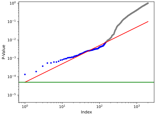
13.6.4 A Re-Sampling Approach
The Khan training and test sets are stacked (83 patients); classes 2 and 4 are compared gene by gene.
R ch13_lab.R
x <- rbind(Khan$xtrain, Khan$xtest)          # 83 patients, 2,308 genes
y <- c(as.numeric(Khan$ytrain), as.numeric(Khan$ytest))
dim(x); table(y)                             # classes 1-4: 11, 29, 18, 25 patients
x <- as.matrix(x)
x1 <- x[which(y == 2), ]
x2 <- x[which(y == 4), ]
n1 <- nrow(x1); n2 <- nrow(x2)
t.out <- t.test(x1[, 11], x2[, 11], var.equal = TRUE)
TT <- t.out$statistic
c(TT, p = t.out$p.value)                     # T = -2.0936, p = 0.0412
Python ch13_lab.py
Kd = pd.read_csv(os.path.join(HERE, "cache", "ch13-Khan.csv"))   # 83 patients: training rows, then test rows
D = Kd.drop(columns="y")
D["Y"] = Kd["y"]
print(D["Y"].value_counts())                  # 2: 29, 4: 25, 3: 18, 1: 11
D2 = D[lambda df: df["Y"] == 2]
D4 = D[lambda df: df["Y"] == 4]
gene_11 = "G0011"
observedT, pvalue = ttest_ind(D2[gene_11], D4[gene_11], equal_var=True)
show("gene 11: T, p =", (round(observedT, 4), round(pvalue, 4)))          # -2.0936, 0.0412
Both: \(T=-2.0936\), \(p=0.0412\). Algorithm 13.3 with \(B=10{,}000\) relabellings:
R ch13_lab.R
# The pooled two-sample t-statistic (13.11), the number t.test(var.equal = TRUE) reports,
# written out so that 10,000 permutations take a fraction of a second.
tstat <- function(a, b) {
  na <- length(a); nb <- length(b)
  s <- sqrt(((na - 1) * var(a) + (nb - 1) * var(b)) / (na + nb - 2))
  (mean(a) - mean(b)) / (s * sqrt(1 / na + 1 / nb))
}
all.equal(unname(tstat(x1[, 11], x2[, 11])), unname(TT))   # TRUE

set.seed(1)
B <- 10000
Tbs <- rep(NA, B)
for (b in 1:B) {                             # Algorithm 13.3: random relabellings of the 54 patients
  dat <- sample(c(x1[, 11], x2[, 11]))
  Tbs[b] <- tstat(dat[1:n1], dat[(n1 + 1):(n1 + n2)])
}
mean(abs(Tbs) >= abs(TT))                    # the re-sampling p-value, 0.0416
Python ch13_lab.py
def tstat_rows(D, n1):
    """Pooled two-sample t-statistic (13.11) for every row of D: the first n1 entries against the rest."""
    a, b = D[:, :n1], D[:, n1:]
    na, nb = a.shape[1], b.shape[1]
    s2 = ((na - 1) * a.var(1, ddof=1) + (nb - 1) * b.var(1, ddof=1)) / (na + nb - 2)
    return (a.mean(1) - b.mean(1)) / np.sqrt(s2 * (1 / na + 1 / nb))
B = 10000
D_ = np.hstack([D2[gene_11], D4[gene_11]])
n_ = D2[gene_11].shape[0]
D_null = D_.copy()
shuffled = np.empty((B, len(D_)))
for b in range(B): # Algorithm 13.3: B random relabellings
rng.shuffle(D_null)
shuffled[b] = D_null
Tnull = tstat_rows(shuffled, n_)
perm_p = (np.abs(Tnull) >= np.abs(observedT)).mean()
show("re-sampling p-value:", perm_p) # 0.0398 (also with > instead of >=)R gives 0.0416 (the R edition's number) and Python 0.0398 (the Python edition's); the Python edition counts \(|T^*|\gt |T|\) rather than \(\ge\), which gives the same value here.
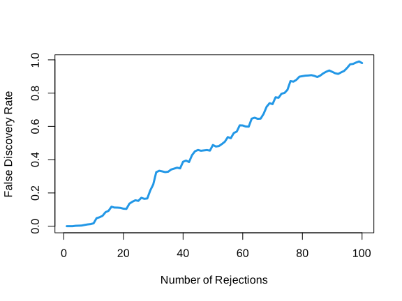
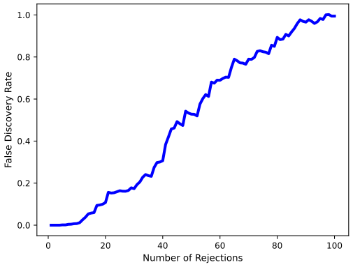
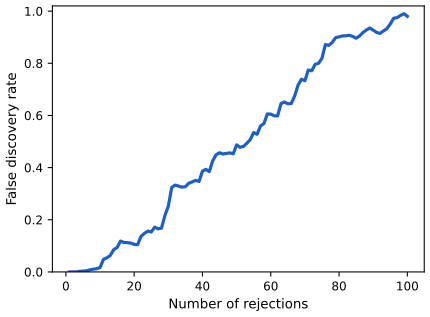
Algorithm 13.4 on 100 randomly chosen genes, each with its own 10,000 relabellings, and the estimated FDR at every threshold \(c\) equal to an observed \(|T|\):
R ch13_lab.R
# Algorithm 13.4 on 100 randomly chosen genes, B = 10,000 relabellings each.
m <- 100
set.seed(1)
index <- sample(ncol(x1), m)
Ts <- rep(NA, m)
Ts.star <- matrix(NA, ncol = m, nrow = B)
for (j in 1:m) {
  k <- index[j]
  Ts[j] <- tstat(x1[, k], x2[, k])
  for (b in 1:B) {
    dat <- sample(c(x1[, k], x2[, k]))
    Ts.star[b, j] <- tstat(dat[1:n1], dat[(n1 + 1):(n1 + n2)])
  }
}
cs <- sort(abs(Ts))                          # the thresholds c: the observed |T| values
FDRs <- Rs <- Vs <- rep(NA, m)
for (j in 1:m) {
  R <- sum(abs(Ts) >= cs[j])
  V <- sum(abs(Ts.star) >= cs[j]) / B        # estimated expected number of false positives
  Rs[j] <- R
  Vs[j] <- V
  FDRs[j] <- V / R
}
max(Rs[FDRs <= 0.1])                         # 15 genes at an estimated FDR of 0.1
sort(index[abs(Ts) >= min(cs[FDRs < 0.1])])
max(Rs[FDRs <= 0.2])                         # 28 genes at 0.2
sort(index[abs(Ts) >= min(cs[FDRs < 0.2])])
Python ch13_lab.py
# Algorithm 13.4 on 100 randomly chosen genes, B = 10,000 relabellings each
m, B = 100, 10000
idx = rng.choice(Kd.columns[1:], m, replace=False)
T_vals = np.empty(m)
Tnull_vals = np.empty((m, B))
for j in range(m):
    col = idx[j]
    T_vals[j] = ttest_ind(D2[col], D4[col], equal_var=True).statistic
    D_ = np.hstack([D2[col], D4[col]])
    D_null = D_.copy()
    for b in range(B):
        rng.shuffle(D_null)
        shuffled[b] = D_null
    Tnull_vals[j] = tstat_rows(shuffled, n_)
cutoffs = np.sort(np.abs(T_vals))
FDRs, Rs, Vs = np.empty((3, m))
for j in range(m):
    R = np.sum(np.abs(T_vals) >= cutoffs[j])
    V = np.sum(np.abs(Tnull_vals) >= cutoffs[j]) / B
    Rs[j], Vs[j], FDRs[j] = R, V, V / R
show("rejections at estimated FDR 0.1 and 0.2:", (Rs[FDRs <= 0.1].max(), Rs[FDRs <= 0.2].max()))   # 15 28
genes01 = sorted(idx[np.abs(T_vals) >= cutoffs[FDRs < 0.1].min()])
show("genes at FDR 0.1:", genes01)| genes rejected at estimated FDR 0.1 | at 0.2 | |
|---|---|---|
R (set.seed(1), the R edition's 100 genes) | 15 | 28 |
Python (default_rng(12), the Python edition's 100 genes) | 19 | 31 |
R reproduces the R edition exactly, including the list of the 15 genes (29, 465, 501, 554, 573, 729, 733, 1301, 1317, 1640, 1646, 1706, 1799, 1942, 2159) and the 28. The Python generator draws a different set of 100 genes, so its counts differ; the Python edition's text repeats the R edition's 15 and 28, which its code does not produce (Notes on the book, 4). With 10% of 15 to 19 rejections, one or two false discoveries are expected.
khan_permutations) instead of separate relabellings per gene: again 15 genes at an estimated FDR of 0.1 and 28 at 0.2. Code: fig_13_11. Reproduces James et al. (2021), Figure 13.11. Download: PDF · SVGFinally, gene 877 (Figure 13.8), beyond the book's lab:
R ch13_lab.R
# Beyond the book's lab: the gene of Figure 13.8, whose null distribution is far from t_52.
T877 <- tstat(x1[, 877], x2[, 877])
Tb877 <- replicate(B, { dat <- sample(c(x1[, 877], x2[, 877])); tstat(dat[1:n1], dat[(n1 + 1):(n1 + n2)]) })
c(T = T877, p_t = 2 * pt(-abs(T877), n1 + n2 - 2), p_perm = mean(abs(Tb877) >= abs(T877)))   # 0.571 against 0.67
Python ch13_lab.py
# Beyond the book's lab: gene 877 (Figure 13.8), whose null distribution is far from t_52.
D_ = np.hstack([D2["G0877"], D4["G0877"]])
T877 = ttest_ind(D2["G0877"], D4["G0877"], equal_var=True)
D_null = D_.copy()
for b in range(B):
    rng.shuffle(D_null)
    shuffled[b] = D_null
perm877 = (np.abs(tstat_rows(shuffled, n_)) >= abs(T877.statistic)).mean()
show("gene 877: T, t p-value, re-sampling p-value:", np.round([T877.statistic, T877.pvalue, perm877], 4))
\(T=-0.5696\) and \(p=0.5714\) in both; the permutation p-values are 0.680 (R) and 0.677 (Python).
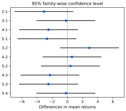
tukey_hsd, the Tukey–Kramer form, which reduces to Tukey's for equal group sizes). All contain zero. Code: fig_13_10. Reproduces James et al. (2021), Figure 13.10 (the R edition's version; the Python edition shows one interval per manager, as in the lab figure above). Download: PDF · SVGNotes on the book
Points where the text or the code of one of the editions disagrees with a computation, with the evidence. None changes the chapter's message.
1. R edition, Section 13.3.2: Holm's third threshold R edition p. 566
The text gives \(p_{(3)}=0.601\gt 0.05/(5+1-3)=0.167\). The threshold is \(0.05/3=0.0167\); the conclusion (\(L=3\)) is unchanged. The Python edition prints 0.0167.
2. Both editions, Section 13.3.2: the p-value 0.0349 for Managers One and Two p. 568
"A two-sample t-test (13.1) for \(H_0:\mu_1=\mu_2\) yields a p-value of 0.0349." The pooled two-sample statistic is \(t=2.170\) with \(50+50-2=98\) degrees of freedom, giving \(p=0.0324\) (Welch's test also gives 0.0324; the paired test of the lab gives 0.038). The book's 0.0349 is, to rounding, what the same \(t=2.170\) gives with 49 degrees of freedom, those of the paired or one-sample test (0.03485). The argument of the paragraph is unaffected.
3. Both editions, Sections 13.5.1 and 13.6.4: which tumours are classes 2 and 4 of Khan pp. 577, 588; Figure 13.9
The books call class 2 (29 patients) rhabdomyosarcoma and class 4 (25 patients) Burkitt's lymphoma. The class sizes in the ISLR2 data are 8, 23, 12, 20 in the training set and 3, 6, 6, 5 in the test set. In Khan et al. (2001) the 63 training samples are 8 Burkitt's lymphoma (BL), 23 Ewing's sarcoma (EWS), 12 neuroblastoma (NB) and 20 rhabdomyosarcoma (RMS), and the 20 tumour test samples 3 BL, 6 EWS, 6 NB and 5 RMS. The class codes 1–4 thus follow the alphabetical order BL, EWS, NB, RMS, and the comparison is Ewing's sarcoma (class 2) against rhabdomyosarcoma (class 4). The same paragraph calls the tumours "small round blood cell tumors"; the established name is small round blue cell tumours (after their appearance under the standard stain). The statistics are unaffected.
4. Python edition, Section 13.6.4: "we reject 15 of the 100 null hypotheses ... 28 genes" Python edition p. 592
The Python lab draws its 100 genes with rng.choice(), which cannot give the R edition's genes, but the text repeats the R edition's 15 and 28, and the code that would print them is not shown. Running the printed code with the same generator (our run reproduces the edition's previous output, 0.0398, exactly, so the generator is in the same state) gives 19 genes at an estimated FDR of 0.1 and 31 at 0.2.
5. Python edition, Section 13.6.3: the BH code marks 145 managers, not 146 Python edition p. 589, In[21]
The hand-coded BH uses selected_ = fund_pvalues < sorted_[sorted_set_].max(), a strict inequality that excludes the \(L\)-th p-value itself, and np.arange(sorted_set_.max()), which stops one index short. Both mark 145 managers, while BH (and the edition's own multipletests output) rejects 146. The fix is <= and np.arange(sorted_set_.max() + 1).
6. Smaller points
- Both labs, Section 13.6.4: "We compute the fraction of the time that our observed test statistic exceeds the test statistics obtained via re-sampling" describes the reverse of the code, which computes the fraction of re-sampled statistics at least as large in absolute value as the observed one, (13.12).
- Python edition, In[25]:
(np.abs(Tnull) > np.abs(observedT)).mean()uses \(>\) where (13.12) has \(\ge\) (no difference here). In[8]:np.linspace(1, 501)gives 50 non-integer values of \(m\) between 1 and 501 rather than \(m=1,\dots,500\) (harmless for the plot). - Section 13.4.2: "As long as the m p-values are independent or only mildly dependent" is vaguer than the theorem: the guarantee is \(\FDR\le q\,m_0/m\) under independence or positive regression dependence; for arbitrary dependence the level must be divided by \(\sum_{k\le m}1/k\) (Result 13.5).
- Section 13.5.1 builds the permutation test on "the distributions of X and Y are the same" but states the null as \(\E(X)=\E(Y)\); the two differ, and the permutation test is exact only for the first (Filling the gap 13.12). (13.12) can return 0, which is not a valid p-value at small levels; \((1+\#)/(B+1)\) is.
- R edition, Table 13.4: the caption says "Exercise 4 in Section 13.6"; the exercises are Section 13.7 (the Python edition says "Exercise 4"). R edition, Exercise 6(c)–(d): for one data set the quantity is the false discovery proportion, as the Python edition says; the false discovery rate is its expectation.
Exercises
All eight exercises of Chapter 13 (R edition pp. 591–595, Python edition pp. 593–596), restated in my own words, with solutions (hidden). The applied solutions are given in R and in Python side by side; the code is that of the two lab files, and the results are those they print.
Conceptual
Exercise 13.1. All \(m\) null hypotheses are true and each is tested at level \(\alpha\). (a) How many Type I errors do we expect? (b) What is the FWER if the tests are independent? (c) With \(m=2\) and positively correlated p-values, how does the FWER compare with (b)? (Think of perfectly correlated p-values first.) (d) And with negatively correlated p-values? (Think of the case where at most one can be below \(\alpha\).)
Solution
(a) \(\E V=\sum_j\Pr(p_j\le\alpha)=m\alpha\), by linearity of expectation, whatever the dependence. (b) \(1-(1-\alpha)^m\) (Result 13.2). (c) Smaller: in the extreme \(p_1=p_2\), \(\FWER=\Pr(p_1\le\alpha)=\alpha\lt 1-(1-\alpha)^2=2\alpha-\alpha^2\). Positive dependence makes the two rejection events overlap, and their union shrinks. (d) Larger: if the rejection events are disjoint (e.g. \(p_2=1-p_1\), \(\alpha\le0.5\)), \(\FWER=\Pr(A_1)+\Pr(A_2)=2\alpha\gt 2\alpha-\alpha^2\), the largest value possible by the union bound (Filling the gap 13.5). The demonstration shows case (c) with correlation 0.9.
Exercise 13.2. Again all \(m\) nulls are true and tested at level \(\alpha\), and now the p-values are independent. Let \(A_j=1\) if \(H_{0j}\) is rejected. (a) What is the distribution of \(A_j\)? (b) Of \(\sum_jA_j\)? (c) What is the standard deviation of the number of Type I errors?
Solution
(a) Bernoulli with success probability \(\Pr(p_j\le\alpha)=\alpha\) (Result 13.1, for a continuous null distribution; at most \(\alpha\) for a discrete one). (b) A sum of \(m\) independent Bernoulli(\(\alpha\)) variables is Binomial\((m,\alpha)\). (c) \(\sqrt{m\alpha(1-\alpha)}\): for \(m=2000\), \(\alpha=0.05\), the number of false rejections is \(100\pm9.7\).
Exercise 13.3. Each \(H_{0j}\) is tested at its own level \(\alpha_j\). Show that \(\FWER\le\sum_j\alpha_j\).
Solution
The FWER is the probability of the union of the events \(A_j=\{H_{0j}\text{ rejected}\}\) over the true nulls; the union bound gives \(\FWER\le\sum_{j\in\mathcal H_0}\Pr(A_j)\le\sum_{j\in\mathcal H_0}\alpha_j\le\sum_{j=1}^m\alpha_j\) (Result 13.3). Bonferroni is the case \(\alpha_j=\alpha/m\); unequal \(\alpha_j\) (weighted Bonferroni) spend the error budget where power is most wanted.
Exercise 13.4. Ten hypotheses have p-values 0.0011, 0.031, 0.017, 0.32, 0.11, 0.90, 0.07, 0.006, 0.004, 0.0009 (\(H_{01}\) to \(H_{10}\), Table 13.4). Which are rejected (a) at level 0.05 without correction, (b) with the FWER controlled at 0.05, (c) with the FDR controlled at 0.05, (d) at FDR 0.2? (e) About how many of the rejections in (d) are false?
Solution
Sorted: 0.0009 (\(H_{10}\)), 0.0011 (\(H_{01}\)), 0.004 (\(H_{09}\)), 0.006 (\(H_{08}\)), 0.017 (\(H_{03}\)), 0.031 (\(H_{02}\)), 0.07 (\(H_{07}\)), 0.11 (\(H_{05}\)), 0.32 (\(H_{04}\)), 0.90 (\(H_{06}\)).
(a) \(p\le0.05\): \(H_{01},H_{02},H_{03},H_{08},H_{09},H_{10}\). (b) Bonferroni (0.005): \(H_{01},H_{09},H_{10}\). Holm does better: the thresholds 0.005, 0.00556, 0.00625, 0.00714, 0.00833 accept the first four sorted p-values and fail at 0.017, so Holm rejects \(H_{01},H_{08},H_{09},H_{10}\), also with FWER at most 0.05. (c) BH thresholds \(0.005j\): \(p_{(5)}=0.017\le0.025\) but \(p_{(6)}=0.031\gt 0.030\) and no later one passes, so \(L=5\): \(H_{01},H_{03},H_{08},H_{09},H_{10}\). (d) Thresholds \(0.02j\): \(p_{(8)}=0.11\le0.16\), \(p_{(9)}=0.32\gt 0.18\), \(p_{(10)}=0.90\gt 0.2\), so \(L=8\): all except \(H_{04}\) and \(H_{06}\). (e) On average at most \(q\,m_0/m\) of the rejections are false, so about \(0.2\times8=1.6\) or fewer: one or two. Both labs' functions (
p.adjust,multipletests, andholm,bhin the code) give these sets.Exercise 13.5. At FWER level 0.1, give five p-values for which (a) Bonferroni and Holm each reject exactly one hypothesis, (b) Bonferroni rejects one and Holm more than one.
Solution
Bonferroni's threshold is 0.02; Holm's are 0.02, 0.025, 0.0333, 0.05, 0.1. (a) 0.01, 0.5, 0.6, 0.7, 0.8: Bonferroni rejects 0.01; Holm rejects 0.01 and stops at 0.5 > 0.025. (b) 0.01, 0.022, 0.5, 0.6, 0.7: Bonferroni rejects only 0.01 (0.022 > 0.02); Holm rejects 0.01 and 0.022 (\(\le0.025\)) and stops at 0.5. Any p-value in \((0.02,0.025]\) in second place works.
Exercise 13.6. For each panel of Figure 13.3: (a) count the false positives, false negatives, true positives, true negatives, Type I and Type II errors of Bonferroni at FWER 0.05; (b) the same for Holm; (c), (d) the false discovery proportion of each; (e) how (a) and (c) change with Bonferroni at 0.001.
Solution
For the panels reproduced above (8 false nulls, 2 true nulls each). A false positive is a Type I error and a false negative a Type II error.
panel procedure TP FN (Type II) TN FP (Type I) FDP left Bonferroni 0.05 7 1 2 0 0 Holm 0.05 7 1 2 0 0 Bonferroni 0.001 4 4 2 0 0 centre Bonferroni 0.05 7 1 2 0 0 Holm 0.05 8 0 2 0 0 Bonferroni 0.001 3 5 2 0 0 right Bonferroni 0.05 4 4 2 0 0 Holm 0.05 8 0 2 0 0 Bonferroni 0.001 0 8 2 0 0 The book's panels give the same pattern (its text: 7 and 7 on the left, 7 and 8 in the centre, 3 and 8 on the right, no Type I errors). With no false positives, every FDP is 0. (e) Bonferroni at 0.001 tests each p-value at \(10^{-4}\): there are never more false positives (still 0, FDP still 0), but many more Type II errors. In the right panel no hypothesis is rejected at all, and the FDP is 0 by the convention \(0/0=0\).
Applied
Exercise 13.7. Carseats data. (a) For each quantitative variable other than
Sales, regressSaleson that variable alone and report the p-value of its slope. Which nulls are rejected (b) at level 0.05 without correction, (c) with FWER 0.05, (d) with FDR 0.2?Solution
R ch13_lab.R
# Exercise 7: Sales on each quantitative variable of Carseats, one simple regression at a time.
quant <- c("CompPrice", "Income", "Advertising", "Population", "Price", "Age", "Education")
ex7_p <- sapply(quant, function(v) summary(lm(Carseats$Sales ~ Carseats[[v]]))$coefficients[2, 4])
signif(ex7_p, 3)
names(ex7_p)[ex7_p <= 0.05]                  # (b) no correction
names(ex7_p)[p.adjust(ex7_p, "bonferroni") <= 0.05]   # (c) FWER 0.05 (Holm gives the same)
names(ex7_p)[p.adjust(ex7_p, "holm") <= 0.05]
names(ex7_p)[p.adjust(ex7_p, "BH") <= 0.2]    # (d) FDR 0.2
Python ch13_lab.py
# Exercise 7: Sales on each quantitative variable of Carseats, one simple regression at a time
Carseats = common.isl_data("Carseats")
quant = ["CompPrice", "Income", "Advertising", "Population", "Price", "Age", "Education"]
ex7_p = pd.Series({v: sm.OLS(Carseats["Sales"], sm.add_constant(Carseats[v])).fit().pvalues[v] for v in quant})
print(ex7_p.map("{:.3g}".format))
show("(b) p <= 0.05:", list(ex7_p.index[ex7_p <= 0.05]))
show("(c) Bonferroni:", list(ex7_p.index[mult_test(ex7_p, 0.05, "bonferroni")[0]]))
show("    Holm:", list(ex7_p.index[mult_test(ex7_p, 0.05, "holm")[0]]))
show("(d) BH at 0.2:", list(ex7_p.index[mult_test(ex7_p, 0.2, "fdr_bh")[0]]))
variable CompPrice Income Advertising Population Price Age Education p-value 0.201 0.0023 4.4e−8 0.314 7.6e−21 2.8e−6 0.300 (b)–(d) In every case
Income,Advertising,PriceandAge: their p-values are tiny or, forIncome, 0.0023, below Bonferroni's \(0.05/7=0.0071\); the other three are above 0.2, so even BH at 0.2 (whose fifth threshold is \(0.2\times5/7=0.14\)) stops at four. R and Python agree to all digits. Note that these are marginal (one-variable) tests:CompPricematters a lot oncePriceis in the model (Chapter 3), but not on its own.Exercise 13.8. Simulate 20 months of returns for 100 managers with no skill (all entries standard normal). (a) Test each mean against zero and plot the p-values. How many nulls are rejected (b) at 0.05 without correction, (c) with FWER 0.05, (d) with FDR 0.05? (e) Now keep only the ten managers with the best average returns and control the FWER, then the FDR, at 0.05 for these ten. (f) Why is (e) misleading?
Solution
R ch13_lab.R
# Exercise 8: 100 simulated managers with no skill at all, 20 months each.
set.seed(1)
n <- 20
m <- 100
X <- matrix(rnorm(n * m), ncol = m)
ex8_p <- apply(X, 2, function(col) t.test(col, mu = 0)$p.value)
save_plot("lab-r-ex8", 6, 4.5, function() hist(ex8_p, breaks = 20, main = "", xlab = "p-value", col = "grey80"))
ex8 <- c(raw = sum(ex8_p <= 0.05), holm = sum(p.adjust(ex8_p, "holm") <= 0.05),
         bh = sum(p.adjust(ex8_p, "BH") <= 0.05))
ex8                                          # (b) a few false rejections; (c), (d) none
best <- order(colMeans(X), decreasing = TRUE)[1:10]   # (e) cherry-pick the 10 best managers
p_best <- ex8_p[best]
ex8_cherry <- c(holm = sum(p.adjust(p_best, "holm") <= 0.05), bh = sum(p.adjust(p_best, "BH") <= 0.05))
ex8_cherry
Python ch13_lab.py
# Exercise 8: 100 simulated managers with no skill, 20 months each rng = np.random.default_rng(1) n, m = 20, 100 X = rng.normal(size=(n, m)) ex8_p = ttest_1samp(X, 0).pvalue fig, ax = plt.subplots(figsize=(6, 4.5)) ax.hist(ex8_p, bins=20, color="0.8", edgecolor="k") ax.set_xlabel("p-value") save(fig, "lab-py-ex8") ex8 = [(ex8_p <= 0.05).sum(), mult_test(ex8_p, 0.05, "holm")[0].sum(), mult_test(ex8_p, 0.05, "fdr_bh")[0].sum()] show("(b)-(d) raw, Holm, BH:", ex8) best = np.argsort(-X.mean(0))[:10] # (e) cherry-pick the ten best managers ex8_cherry = [mult_test(ex8_p[best], 0.05, "holm")[0].sum(), mult_test(ex8_p[best], 0.05, "fdr_bh")[0].sum()] show("(e) cherry-picked ten, Holm and BH:", ex8_cherry)(a) Both histograms are roughly flat, as they must be when every null is true (Result 13.1). (b) Four rejections in each language (expected 5), all false. (c), (d) Holm and BH reject nothing. (e) Cherry-picking the ten best managers and correcting only for ten tests: R rejects one manager with Holm and one with BH (the best ten include a p-value of 0.0034, below \(0.05/10\)); Python rejects none (its best ten start at 0.0096; its smallest p-value overall, 0.0008, belongs to a manager with a negative mean). (f) The correction assumes that the ten tests were chosen before seeing the data. Choosing the ten smallest p-values out of 100 makes them the smallest order statistics of 100 uniforms, far from uniform themselves: correcting for 10 tests treats \(m=10\) when the selection used \(m=100\), so the FWER and FDR guarantees are lost. The honest correction is for all 100 tests, as in (c) and (d).
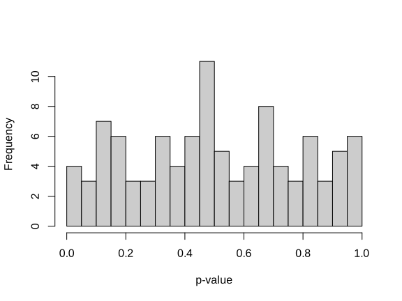
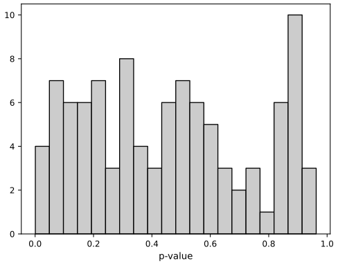
Demonstrations for this chapter
Each demonstration runs in the browser and links back to these notes. The ▶ Demo boxes above open them already set to the case under discussion.
| Demonstration | What you can see | Sections and results |
|---|---|---|
| The FWER: Bonferroni and Holm | The exact FWER curve against \(m\); the sorted p-values of one simulated family with Bonferroni's level and Holm's thresholds; simulated FWER and power of no correction, Bonferroni and Holm, for any \(m\), \(\alpha\), share of true nulls, effect size and correlation. Presets: 1 100 uncorrected tests (Figure 13.2); 2 ten tests, two true nulls (Figure 13.3); 3 500 true nulls, \(1-e^{-\alpha}\); 4 correlated tests; 5 power and \(m\) (Figure 13.5). | 13.3; Results 13.2–13.4, Filling the gap 13.5 |
| Benjamini–Hochberg on the Fund managers | The sorted p-values with the BH line, Bonferroni's level and Holm's thresholds; the estimated FDR \(mp_{(k)}/k\) and the q-values; adjusted p-values for small families. Presets: 1 five managers (Table 13.3); 2 \(q=0.05\), no rejection; 3 \(q=0.1\), 146 managers; 4 \(q=0.3\), 279 against 1; 5 the first 100 managers only. | 13.4; Algorithm 13.2, Result 13.5, Filling the gap 13.11 |
| Permutation null versus the t distribution | Any of the 2,308 Khan genes: its values in the two classes, one relabelling at a time or 10,000, the permutation distribution against \(t_{52}\); the two p-values of every gene; the re-sampling FDR curve against BH. Presets: 1 gene 11 (Figure 13.7); 2 gene 877 (Figure 13.8); 3 one relabelling at a time; 4 gene 1955, beyond the reach of \(B\); 5 the re-sampling FDR (Figure 13.9). | 13.5; Algorithms 13.3, 13.4, Results 13.7, 13.8 |
Related demonstrations elsewhere on the site: FDR control on the airway data, the exact permutation test and p-value hacking (Statistical Methods for Modern Biology). The code for every figure of this page is code/ch13_multiple_testing.py; the lab is code/ch13_lab.R and code/ch13_lab.py (see the code index).
References
- James, G., Witten, D., Hastie, T. and Tibshirani, R. (2021). An Introduction to Statistical Learning with Applications in R, 2nd edition. Springer, New York. Chapter 13, pp. 553–595. www.statlearning.com.
- James, G., Witten, D., Hastie, T., Tibshirani, R. and Taylor, J. (2023). An Introduction to Statistical Learning with Applications in Python. Springer, Cham. Chapter 13, pp. 557–596.
- Benjamini, Y. and Hochberg, Y. (1995). Controlling the false discovery rate: a practical and powerful approach to multiple testing. Journal of the Royal Statistical Society B, 57(1), 289–300.
- Benjamini, Y. and Yekutieli, D. (2001). The control of the false discovery rate in multiple testing under dependency. Annals of Statistics, 29(4), 1165–1188.
- Efron, B. (2010). Large-Scale Inference: Empirical Bayes Methods for Estimation, Testing, and Prediction. Cambridge University Press, Cambridge.
- Hastie, T., Tibshirani, R. and Friedman, J. (2009). The Elements of Statistical Learning, 2nd edition. Springer, New York. Section 18.7.
- Holm, S. (1979). A simple sequentially rejective multiple test procedure. Scandinavian Journal of Statistics, 6(2), 65–70.
- Khan, J., Wei, J. S., Ringnér, M., Saal, L. H., Ladanyi, M., Westermann, F., Berthold, F., Schwab, M., Antonescu, C. R., Peterson, C. and Meltzer, P. S. (2001). Classification and diagnostic prediction of cancers using gene expression profiling and artificial neural networks. Nature Medicine, 7(6), 673–679.
- Scheffé, H. (1953). A method for judging all contrasts in the analysis of variance. Biometrika, 40(1–2), 87–110.
- Storey, J. D. and Tibshirani, R. (2003). Statistical significance for genomewide studies. Proceedings of the National Academy of Sciences, 100(16), 9440–9445.
- Tukey, J. W. (1953). The Problem of Multiple Comparisons. Unpublished manuscript, Princeton University; reprinted in The Collected Works of John W. Tukey, Volume VIII (1994), Chapman and Hall, New York.
- Tusher, V. G., Tibshirani, R. and Chu, G. (2001). Significance analysis of microarrays applied to the ionizing radiation response. Proceedings of the National Academy of Sciences, 98(9), 5116–5121.
- Westfall, P. H. and Young, S. S. (1993). Resampling-Based Multiple Testing. Wiley, New York.
The numerical statements in the text (uniformity of null p-values, the FWER formulas and bounds, Holm's and Tukey's FWER control, Scheffé's identity, FDR control by BH and its equivalence with the plug-in rule, the figures' numbers against the book's, and the lab and exercise results in both languages) were confirmed numerically.