Linear Methods for Regression
Linear regression is the workhorse of statistics and the template for almost everything else in the book. This chapter fits it by least squares and works out exactly how the estimates behave (their Gaussian sampling distribution, the t and F tests, the Gauss–Markov optimality), then asks how to do better than least squares when there are many correlated inputs: by choosing a subset of them, by shrinking the coefficients (ridge regression and the lasso), by regressing on a few derived directions (principal components and partial least squares), or by following a whole path of solutions (least angle regression, forward stagewise regression, coordinate descent). The prostate cancer data run through the chapter, and every table and coefficient profile of the book is reproduced here.
Ch. 1 Introduction Ch. 2 Supervised learning Ch. 3 Linear regression Ch. 4 Linear classification Ch. 5 Basis expansions Ch. 6 Kernel smoothing Ch. 7 Model assessment Ch. 8 Inference and averaging Ch. 9 Additive models and trees Ch. 10 Boosting Ch. 11 Neural networks Ch. 12 SVMs Ch. 13 Nearest neighbours Ch. 14 Unsupervised learning Ch. 15 Random forests Ch. 16 Ensembles Ch. 17 Graphical models Ch. 18 High-dimensional problems
How to read these notes
They follow the book. Sections carry the book's numbers (3.2, 3.4.1, ...) and every displayed equation that appears in the book carries the book's own equation number, e.g. \((3.44)\), so the notes can be read next to the book. Equations without a number are steps the book skips.
Filling the gaps. Wherever the book says that a result "is easy to show", "can be shown", or leaves it to an exercise, an orange Filling the gap box or a proof gives the complete argument. Proofs and derivations start hidden: open one with its bar, or use the button below.
Figures, tables and demonstrations. All twenty figures of the chapter, the panel of Table 3.4 and Tables 3.1–3.3 are recomputed from scratch by the Python code; the two geometric pictures (Figures 3.2 and 3.4) are drawn from explicitly computed projections. The ▶ Demo boxes open an interactive demonstration already set to the case being discussed.
Main reference
T. Hastie, R. Tibshirani and J. Friedman, The Elements of Statistical Learning: Data Mining, Inference, and Prediction, 2nd edition, Springer (2009), Chapter 3, pages 43–99 (book website, with the data sets: hastie.su.domains/ElemStatLearn). Section, equation, figure, table and exercise numbers below refer to this book. Further reading is listed in the references.
The explanations, derivations, figures and code are my own; equations are cited by their numbers in the book.
Companion courses
Parts of this chapter are also treated, from a different angle, in two companion courses on this site:
- Bayesian and Probabilistic Machine Learning (Bishop 2006): least squares as maximum likelihood and its geometry, Sections 3.1.1–3.1.2; regularised least squares, ridge and the lasso picture, Section 3.1.4; multiple outputs, Section 3.1.5; the bias–variance decomposition, Section 3.2; ridge as a posterior mode and the lasso as a MAP estimate, Result 3.11 and Filling the gap 3.6; the effective number of parameters, Section 3.5.3.
- Foundations of Deep Learning (Bishop and Bishop 2024): the normal equations, the pseudo-inverse and conditioning, Sections 4.1.3–4.1.4; ridge regression through the SVD, Result 4.7; L1 versus L2 penalties and why the lasso gives exact zeros, Section 9.2.2 and Filling the gap 9.5; weight decay and the effective number of parameters, Result 9.4. Demonstrations of related ideas: L1 versus L2 paths, basis-function regression.
Where a proof there is the same, these notes state the result, give a short argument and link to the full derivation. New here: the exact sampling theory behind the t and F tests, the Gauss–Markov theorem, Gram–Schmidt and QR, subset and stepwise selection, the lasso's optimality conditions and its path, least angle regression and its degrees of freedom, principal components regression, partial least squares (including why it can inflate some components), reduced-rank regression, and the path algorithms of Section 3.8.
The chapter at a glance
- 3.2 Least squares projects \(\by\) onto the column space of \(\bX\) (Result 3.2). Under Gaussian errors \(\hb\) is Gaussian, \(\hat\sigma^2\) is a scaled \(\chi^2\) and the two are independent (Result 3.4), which gives the t and F tests (Result 3.5). Least squares is the best linear unbiased estimator (Result 3.6), and each multiple-regression coefficient is a simple regression on an adjusted input (Result 3.8).
- 3.3 Best-subset, forward- and backward-stepwise and forward-stagewise selection; on the prostate data the first three agree, and cross-validation picks {lcavol, lweight}.
- 3.4 Ridge regression shrinks the coordinates of \(\by\) along the principal components by \(d_j^2/(d_j^2+\lambda)\) and has \(\df(\lambda)=\sum_jd_j^2/(d_j^2+\lambda)\) degrees of freedom (Result 3.13). The lasso is characterised by its optimality conditions (Result 3.16), soft-thresholds under orthonormal inputs (Result 3.17), and its whole path is computed by least angle regression with one modification (Result 3.19). Its degrees of freedom are the expected number of nonzero coefficients (Result 3.20).
- 3.5–3.6 Principal components regression truncates the components that ridge shrinks; partial least squares is the conjugate gradient method in disguise and applies polynomial shrinkage factors that can exceed 1 (Result 3.23).
- 3.7 Reduced-rank regression is least squares followed by a projection onto the leading canonical response directions (Result 3.25).
- 3.8–3.9 Incremental forward stagewise regression, piecewise-linear paths, the Dantzig selector, the grouped lasso, non-convex penalties and pathwise coordinate descent; how the computations are done.
Notation. Training data \((\bx_i,y_i)\), \(i=1,\dots,N\), with \(\bx_i\in\R^p\). \(\bX\) is the \(N\times(p+1)\) matrix with rows \((1,\bx_i^\T)\) in Section 3.2, and the \(N\times p\) matrix of centred inputs from Section 3.4 on (the book switches at (3.43); so do we, and say so). \(\by=(y_1,\dots,y_N)^\T\), \(\langle\ba,\mathbf{b}\rangle=\ba^\T\mathbf{b}\), \(\|\cdot\|\) is the Euclidean norm, \(\bone\) the vector of ones. Gradients are column vectors.
Prerequisites. Chapter 2 of the book (least squares versus nearest neighbours, the bias–variance view), multivariate Gaussian distributions, and the singular value decomposition and matrix calculus of the companion course's toolkit.
3.1 Introduction
p. 43 A linear regression model assumes that the regression function \(\E(Y\given X)\) is linear in the inputs \(X_1,\dots,X_p\), or at least that a linear function is a reasonable approximation to it. Linear models are simple and interpretable, they can beat flexible methods when there are few cases, much noise or sparse data, and they become very flexible once applied to transformed inputs (the basis expansions of Chapter 5). Almost every nonlinear method later in the book generalises one of the ideas of this chapter, which is why it is worth understanding them exactly.
3.2 Linear Regression Models and Least Squares
Definition 3.1 (the linear model and least squares) pp. 44–45, (3.1)–(3.3)
With an input vector \(X^\T=(X_1,\dots,X_p)\) the linear regression model is
\[ f(X)=\beta_0+\sum_{j=1}^pX_j\beta_j. \tag{3.1} \]The inputs may be raw measurements, transformations (log, square root), basis expansions (\(X_2=X_1^2\)), dummy codes for the levels of a qualitative input, or interactions (\(X_3=X_1X_2\)): the model is linear in the parameters, whatever the inputs. Least squares chooses \(\bb=(\beta_0,\dots,\beta_p)^\T\) to minimise the residual sum of squares
\[ \RSS(\bb)=\sum_{i=1}^N\big(y_i-f(x_i)\big)^2=\sum_{i=1}^N\Big(y_i-\beta_0-\sum_{j=1}^px_{ij}\beta_j\Big)^2, \tag{3.2} \] \[ \RSS(\bb)=(\by-\bX\bb)^\T(\by-\bX\bb), \tag{3.3} \]where \(\bX\) is \(N\times(p+1)\) with a column of ones first. The criterion is sensible when the \(y_i\) are conditionally independent given the inputs; it makes no assumption that (3.1) is true.
Result 3.1 (the normal equations) p. 45, (3.4)–(3.6)
\(\RSS\) is a convex quadratic with
\[ \frac{\partial\RSS}{\partial\bb}=-2\bX^\T(\by-\bX\bb),\qquad \frac{\partial^2\RSS}{\partial\bb\,\partial\bb^\T}=2\bX^\T\bX. \tag{3.4} \]Its minimisers are exactly the solutions of the normal equations
\[ \bX^\T(\by-\bX\bb)=\mathbf{0}. \tag{3.5} \]If \(\bX\) has full column rank \(p+1\) then \(\bX^\T\bX\) is positive definite and the minimiser is unique:
\[ \hb=(\bX^\T\bX)^{-1}\bX^\T\by. \tag{3.6} \]Without full rank the minimisers form an affine set, all with the same fitted vector \(\bX\hb\).
Proof (short; the full argument is in the companion course)
For any \(\bb^\star\) solving (3.5) and any \(\bv\), expanding the square gives the exact identity \[ \RSS(\bb^\star+\bv)=\RSS(\bb^\star)-2\bv^\T\bX^\T(\by-\bX\bb^\star)+\|\bX\bv\|^2=\RSS(\bb^\star)+\|\bX\bv\|^2 \]. So every solution of (3.5) is a global minimiser, and \(\bb^\star+\bv\) is another minimiser iff \(\bX\bv=\mathbf{0}\), which leaves \(\bX\bb\) unchanged. Conversely a minimiser has zero gradient. A solution of (3.5) always exists because \(\bX^\T\by\) lies in the column space of \(\bX^\T\), which equals that of \(\bX^\T\bX\). With full column rank, \(\bv^\T\bX^\T\bX\bv=\|\bX\bv\|^2>0\) for \(\bv\ne\mathbf{0}\), so \(\bX^\T\bX\) is invertible and (3.6) follows. Full details, including the pseudo-inverse: Foundations of Deep Learning, Result 4.2. ∎
See also (companion courses): least squares as maximum likelihood; the normal equations and the pseudo-inverse.
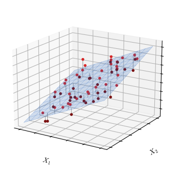
fig_3_1. Reproduces Hastie, Tibshirani and Friedman (2009), Figure 3.1. Download: PDF · SVGp. 46 The fitted values at the training inputs are
\[ \hat\by=\bX\hb=\bX(\bX^\T\bX)^{-1}\bX^\T\by, \tag{3.7} \]and \(\bH=\bX(\bX^\T\bX)^{-1}\bX^\T\), the hat matrix, "puts the hat on \(\by\)". The prediction at a new input is \(\hat f(x_0)=(1,x_0^\T)\hb\).
Result 3.2 (the hat matrix is an orthogonal projection) p. 46, Figure 3.2
If \(\bX\) has full column rank, \(\bH\) is symmetric and idempotent (\(\bH^2=\bH\)), its eigenvalues are 1 (with multiplicity \(p+1\)) and 0, \(\tr\bH=p+1\), and \(\bH\by\) is the point of the column space \(\col(\bX)\) closest to \(\by\). The residual \(\by-\hat\by=(\bI-\bH)\by\) is orthogonal to every column of \(\bX\), and \(\bI-\bH\) is the projection onto the orthogonal complement, of rank \(N-p-1\). Without full rank the same holds with \(\bH=\bX\bX^{+}\) (pseudo-inverse) and \(\tr\bH=\rank\bX\).
Proof
Symmetry: \(\bH^\T=\bX\big((\bX^\T\bX)^{-1}\big)^\T\bX^\T=\bH\) since \(\bX^\T\bX\) is symmetric. Idempotence: \[ \bH^2=\bX(\bX^\T\bX)^{-1}\bX^\T\bX(\bX^\T\bX)^{-1}\bX^\T=\bH \]. If \(\bH\bv=\mu\bv\) with \(\bv\ne\mathbf{0}\) then \(\mu\bv=\bH^2\bv=\mu^2\bv\), so \(\mu\in\{0,1\}\); a symmetric matrix is diagonalisable, so \(\tr\bH=\rank\bH\), and by the cyclic property \[ \tr\bH=\tr\big((\bX^\T\bX)^{-1}\bX^\T\bX\big)=\tr\bI_{p+1}=p+1 \]. For any \(\bb\), \(\by-\bX\bb=(\by-\bH\by)+\bX(\hb-\bb)\) with the two parts orthogonal because \(\bX^\T(\by-\bH\by)=\mathbf{0}\) is (3.5); Pythagoras gives \[ \|\by-\bX\bb\|^2=\|\by-\hat\by\|^2+\|\bX(\hb-\bb)\|^2 \], so \(\hat\by\) is the closest point. \(\bI-\bH\) is symmetric and idempotent with trace \(N-p-1\). The rank-deficient case is Result 4.3 of the companion course. ∎
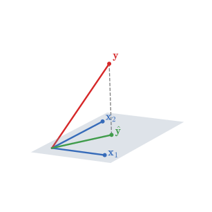
See also (companion course): least squares is an orthogonal projection.
p. 47 To say how precise \(\hb\) is, assume now that the \(y_i\) are uncorrelated with constant variance \(\sigma^2\) and that the \(x_i\) are fixed.
Result 3.3 (moments of \(\hb\) and \(\hat\sigma^2\)) p. 47, (3.8)
If \(\E\by=\bX\bb\) and \(\Var(\by)=\sigma^2\bI\), then \(\E\hb=\bb\) and
\[ \Var(\hb)=(\bX^\T\bX)^{-1}\sigma^2. \tag{3.8} \]The estimate \(\hat\sigma^2=\frac{1}{N-p-1}\sum_{i=1}^N(y_i-\hat y_i)^2\) is unbiased: \(\E\hat\sigma^2=\sigma^2\).
Proof
\(\hb=\mathbf{A}\by\) with \(\mathbf{A}=(\bX^\T\bX)^{-1}\bX^\T\), so \(\E\hb=\mathbf{A}\bX\bb=\bb\) and \[ \Var(\hb)=\mathbf{A}(\sigma^2\bI)\mathbf{A}^\T=\sigma^2(\bX^\T\bX)^{-1}\bX^\T\bX(\bX^\T\bX)^{-1}=\sigma^2(\bX^\T\bX)^{-1} \]. For the variance estimate write \(\be=\by-\bX\bb\), so \(\E\be=\mathbf{0}\), \(\E\be\be^\T=\sigma^2\bI\), and the residual is \((\bI-\bH)\by=(\bI-\bH)\be\) because \((\bI-\bH)\bX=\mathbf{0}\). Then
\[ \E\|(\bI-\bH)\be\|^2=\E\,\be^\T(\bI-\bH)\be=\E\tr\big((\bI-\bH)\be\be^\T\big)=\sigma^2\tr(\bI-\bH)=\sigma^2(N-p-1), \]using that \(\bI-\bH\) is symmetric idempotent (Result 3.2). Divide by \(N-p-1\). ∎
For tests and intervals the book adds two assumptions: the mean really is linear, and the deviations are additive and Gaussian,
\[ Y=\E(Y\given X_1,\dots,X_p)+\varepsilon=\beta_0+\sum_{j=1}^pX_j\beta_j+\varepsilon,\qquad \varepsilon\sim\N(0,\sigma^2). \tag{3.9} \]Result 3.4 (the sampling distribution of \(\hb\) and \(\hat\sigma^2\)) p. 47, (3.10)–(3.11)
Under (3.9) with independent errors and fixed full-rank \(\bX\),
\[ \hb\sim\N\big(\bb,(\bX^\T\bX)^{-1}\sigma^2\big), \tag{3.10} \] \[ (N-p-1)\hat\sigma^2\sim\sigma^2\chi^2_{N-p-1}, \tag{3.11} \]and \(\hb\) and \(\hat\sigma^2\) are independent.
Filling the gap 3.1: why (3.10), (3.11) and independence hold p. 47, "it is easy to show"
The whole argument rests on two facts about Gaussian vectors: linear maps of them are Gaussian, and uncorrelated jointly Gaussian blocks are independent.
Derivation
Setting. \(\by=\bX\bb+\be\) with \(\be\sim\N(\mathbf{0},\sigma^2\bI_N)\). Write \(n=p+1\) and \(\bH\) for the hat matrix.
(3.10). \(\hb=\bb+\mathbf{A}\be\) with \(\mathbf{A}=(\bX^\T\bX)^{-1}\bX^\T\): an affine function of a Gaussian vector, hence Gaussian, with the mean and covariance of Result 3.3.
Independence. Stack \(\hb-\bb=\mathbf{A}\be\) and the residual \(\mathbf{e}=(\bI-\bH)\be\). The stacked vector is a linear map of \(\be\), so it is jointly Gaussian, and the cross-covariance is \[ \Cov(\mathbf{A}\be,(\bI-\bH)\be)=\sigma^2\mathbf{A}(\bI-\bH)=\sigma^2(\bX^\T\bX)^{-1}\big(\bX^\T-\bX^\T\bH\big)=\mathbf{0} \], since \(\bX^\T\bH=\bX^\T\). Jointly Gaussian and uncorrelated means independent. Hence \(\hb\) is independent of \(\mathbf{e}\), and therefore of any function of \(\mathbf{e}\), in particular of \(\hat\sigma^2=\|\mathbf{e}\|^2/(N-n)\).
(3.11). Diagonalise the projection: \(\bI-\bH=\mathbf{O}\diag(1,\dots,1,0,\dots,0)\mathbf{O}^\T\) with \(\mathbf{O}\) orthogonal and \(N-n\) ones (Result 3.2). Put \(\mathbf{w}=\mathbf{O}^\T\be/\sigma\). Because \(\mathbf{O}\) is orthogonal, \(\mathbf{w}\sim\N(\mathbf{0},\bI_N)\): its coordinates are independent standard normals. Then
\[ \frac{(N-n)\hat\sigma^2}{\sigma^2}=\frac{\be^\T(\bI-\bH)\be}{\sigma^2}=\mathbf{w}^\T\diag(1,\dots,1,0,\dots,0)\mathbf{w}=\sum_{k=1}^{N-n}w_k^2\sim\chi^2_{N-n}, \]by the definition of the chi-squared distribution as a sum of squared independent standard normals. With \(n=p+1\) this is (3.11). ∎
Confirmed numerically on the prostate design (20000 simulated response vectors): the empirical mean and covariance of \(\hb\) match (3.10), a Kolmogorov–Smirnov test does not reject the \(\chi^2_{58}\) law of \(58\hat\sigma^2/\sigma^2\) (p = 0.27), and the correlations between \(\hat\beta_j\) and \(\hat\sigma^2\) are all below 0.02.
Result 3.5 (the t and F tests) pp. 48–49, (3.12)–(3.13); Exercise 3.1
(a) With \(v_j\) the \(j\)th diagonal element of \((\bX^\T\bX)^{-1}\), the Z-score
\[ z_j=\frac{\hat\beta_j}{\hat\sigma\sqrt{v_j}} \tag{3.12} \]has a \(t_{N-p-1}\) distribution when \(\beta_j=0\) (a standard normal if \(\sigma\) is known and replaces \(\hat\sigma\)).
(b) For nested models with \(p_1+1\) and \(p_0+1\) parameters, the smaller obtained by setting \(p_1-p_0\) coefficients to zero,
\[ F=\frac{(\RSS_0-\RSS_1)/(p_1-p_0)}{\RSS_1/(N-p_1-1)} \tag{3.13} \]has an \(F_{p_1-p_0,\,N-p_1-1}\) distribution when the smaller model is correct.
(c) When a single coefficient is dropped (\(p_1-p_0=1\)), \(F=z_j^2\) (Exercise 3.1).
Filling the gap 3.2: deriving the t and F distributions pp. 48–49
Derivation
Definitions. If \(Z\sim\N(0,1)\) and \(V\sim\chi^2_k\) are independent, \(Z/\sqrt{V/k}\) has the \(t_k\) distribution. If \(V_1\sim\chi^2_{k_1}\) and \(V_2\sim\chi^2_{k_2}\) are independent, \((V_1/k_1)/(V_2/k_2)\) has the \(F_{k_1,k_2}\) distribution.
(a) By (3.10), \(\hat\beta_j\sim\N(\beta_j,\sigma^2v_j)\), so under \(\beta_j=0\), \(Z=\hat\beta_j/(\sigma\sqrt{v_j})\sim\N(0,1)\). By (3.11), \(V=(N-p-1)\hat\sigma^2/\sigma^2\sim\chi^2_{N-p-1}\), independent of \(Z\) by Result 3.4. Then \(z_j=Z/\sqrt{V/(N-p-1)}\): the unknown \(\sigma\) cancels, and \(z_j\sim t_{N-p-1}\).
(b) Let \(\bH_1,\bH_0\) be the hat matrices of the big and small models. The column space of the small model lies inside that of the big one, so \(\bH_1\bH_0=\bH_0\bH_1=\bH_0\), and \(\bP=\bH_1-\bH_0\) is symmetric with \(\bP^2=\bH_1-\bH_0-\bH_0+\bH_0=\bP\): a projection, of rank \(\tr\bP=(p_1+1)-(p_0+1)=p_1-p_0\). Moreover \(\bP(\bI-\bH_1)=\mathbf{0}\). Now
\[ \RSS_0-\RSS_1=\|(\bI-\bH_0)\by\|^2-\|(\bI-\bH_1)\by\|^2=\|\bP\by\|^2, \]because \((\bI-\bH_0)\by=\bP\by+(\bI-\bH_1)\by\) is an orthogonal sum. Under the small model \(\bX\bb\in\col(\bX_0)\), so \(\bP\bX\bb=\mathbf{0}\) and \(\bP\by=\bP\be\). Diagonalise \(\bH_1=\mathbf{O}\mathbf{\Lambda}\mathbf{O}^\T\) with an orthonormal basis whose first \(p_0+1\) vectors span \(\col(\bX_0)\) and the next \(p_1-p_0\) complete \(\col(\bX_1)\). With \(\mathbf{w}=\mathbf{O}^\T\be/\sigma\sim\N(\mathbf{0},\bI)\), \(\|\bP\be\|^2/\sigma^2\) is the sum of squares of the \(p_1-p_0\) middle coordinates and \(\RSS_1/\sigma^2\) the sum of squares of the last \(N-p_1-1\): two independent chi-squared variables. Dividing each by its degrees of freedom gives (3.13) with the \(F_{p_1-p_0,N-p_1-1}\) law.
(c) Order the columns so that \(x_j\) is last. By Result 3.8 below, \(\hat\beta_j=\langle\bz,\by\rangle/\|\bz\|^2\) and \(v_j=1/\|\bz\|^2\), where \(\bz\) is \(x_j\) adjusted for all other columns, and \(\bP=\bz\bz^\T/\|\bz\|^2\). So \(\RSS_0-\RSS_1=\langle\bz,\by\rangle^2/\|\bz\|^2=\hat\beta_j^2/v_j\), and \(F=(\hat\beta_j^2/v_j)/\hat\sigma^2=z_j^2\). Since the square of a \(t_k\) variable is \(F_{1,k}\) by the definitions above, the two tests are the same test. ∎
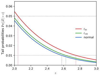
p. 49 Isolating \(\beta_j\) in (3.10) gives the \(1-2\alpha\) interval
\[ \big(\hat\beta_j-z^{(1-\alpha)}v_j^{1/2}\hat\sigma,\ \hat\beta_j+z^{(1-\alpha)}v_j^{1/2}\hat\sigma\big), \tag{3.14} \]with \(z^{(0.975)}=1.96\), \(z^{(0.95)}=1.645\), and an approximate confidence set for the whole vector,
\[ C_\beta=\big\{\bb:\ (\hb-\bb)^\T\bX^\T\bX(\hb-\bb)\le\hat\sigma^2{\chi^2_{p+1}}^{(1-\alpha)}\big\}, \tag{3.15} \]with \({\chi^2_5}^{(0.95)}=11.1\) and \({\chi^2_5}^{(0.90)}=9.2\).
Filling the gap 3.3: the exact versions of (3.14)–(3.15), the band for \(f(x)\), and why the intervals survive non-Gaussian errors p. 49
Derivation
Exact intervals. Under (3.9), replacing \(z^{(1-\alpha)}\) by the \(t_{N-p-1}\) quantile makes (3.14) exact, by Result 3.5(a). For the vector, \((\hb-\bb)^\T\bX^\T\bX(\hb-\bb)/\sigma^2\sim\chi^2_{p+1}\) (it is \(\|\mathbf{L}^\T(\hb-\bb)\|^2/\sigma^2\) with \(\bX^\T\bX=\mathbf{L}\mathbf{L}^\T\), and \(\mathbf{L}^\T(\hb-\bb)/\sigma\sim\N(\mathbf{0},\bI)\)), independent of \(\hat\sigma^2\), so dividing by \((p+1)\hat\sigma^2/\sigma^2\) gives an \(F_{p+1,N-p-1}\) variable. The exact set uses \((p+1)F^{(1-\alpha)}_{p+1,N-p-1}\) in place of \({\chi^2_{p+1}}^{(1-\alpha)}\); the two agree as \(N\to\infty\) because \(kF_{k,m}\to\chi^2_k\) in distribution as \(m\to\infty\).
The band for \(f(x)=x^\T\bb\). Write \(\mathbf{M}=\bX^\T\bX\) and \(c^2=\hat\sigma^2{\chi^2_{p+1}}^{(1-\alpha)}\). For \(\bb\in C_\beta\), by the Cauchy–Schwarz inequality in the inner product defined by \(\mathbf{M}\),
\[ |x^\T(\bb-\hb)|=|(\mathbf{M}^{-1}x)^\T\mathbf{M}(\bb-\hb)|\le\sqrt{x^\T\mathbf{M}^{-1}x}\,\sqrt{(\bb-\hb)^\T\mathbf{M}(\bb-\hb)}\le c\sqrt{x^\T\mathbf{M}^{-1}x}, \]with equality at \(\bb=\hb\pm c\,\mathbf{M}^{-1}x/\sqrt{x^\T\mathbf{M}^{-1}x}\in C_\beta\). So \[ \{x^\T\bb:\bb\in C_\beta\}=x^\T\hb\pm c\sqrt{x^\T\mathbf{M}^{-1}x} \]: the same shape as the pointwise interval, \(x^\T\hb\pm z^{(1-\alpha)}\hat\sigma\sqrt{x^\T\mathbf{M}^{-1}x}\), but with the larger multiplier \(\sqrt{{\chi^2_{p+1}}^{(1-\alpha)}}\). Because the set is a single event of probability \(1-2\alpha\) (approximately), the resulting band covers the whole function simultaneously (Scheffé's method). Exercise 3.2 compares the two bands.
Without Gaussian errors. If the errors are independent with mean 0 and variance \(\sigma^2\) but not Gaussian, \(\hb-\bb=(\bX^\T\bX)^{-1}\bX^\T\be\) is a weighted sum of independent errors. If \(\max_i h_{ii}\to0\) (no single case dominates; \(h_{ii}\) the leverages), the Lindeberg central limit theorem gives \((\bX^\T\bX)^{1/2}(\hb-\bb)/\sigma\to\N(\mathbf{0},\bI)\), and \(\hat\sigma^2\to\sigma^2\) in probability by Result 3.3 and a weak law. By Slutsky's theorem the coverage of (3.14) tends to \(1-2\alpha\), which is the book's claim. ∎
3.2.1 Example: Prostate Cancer
pp. 49–51 The data (Stamey et al., 1989) relate the log of prostate-specific antigen (lpsa) to eight clinical measures of 97 men about to undergo radical prostatectomy: log cancer volume (lcavol), log prostate weight (lweight), age, log benign prostatic hyperplasia (lbph), seminal vesicle invasion (svi, binary), log capsular penetration (lcp), Gleason score (gleason, ordered) and the percentage of Gleason scores 4 or 5 (pgg45). The data file on the book's website marks the random split into 67 training and 30 test cases. The predictors are standardised to unit variance; to reproduce the book's numbers the mean and standard deviation must be those of all 97 men, not of the training set.
Table 3.1. Correlations of the predictors (training set) p. 50
| lcavol | lweight | age | lbph | svi | lcp | gleason | |
|---|---|---|---|---|---|---|---|
| lweight | 0.300 | ||||||
| age | 0.286 | 0.317 | |||||
| lbph | 0.063 | 0.437 | 0.287 | ||||
| svi | 0.593 | 0.181 | 0.129 | −0.139 | |||
| lcp | 0.692 | 0.157 | 0.173 | −0.089 | 0.671 | ||
| gleason | 0.426 | 0.024 | 0.366 | 0.033 | 0.307 | 0.476 | |
| pgg45 | 0.483 | 0.074 | 0.276 | −0.030 | 0.481 | 0.663 | 0.757 |
Recomputed from the 67 training cases; every entry equals the book's. Reproduces Hastie, Tibshirani and Friedman (2009), Table 3.1.
Table 3.2. Least-squares fit to the prostate training data p. 50
| Term | Coefficient | Std. error | Z score |
|---|---|---|---|
| Intercept | 2.465 | 0.089 | 27.60 |
| lcavol | 0.680 | 0.127 | 5.37 |
| lweight | 0.263 | 0.096 | 2.75 |
| age | −0.141 | 0.101 | −1.40 |
| lbph | 0.210 | 0.102 | 2.06 |
| svi | 0.305 | 0.124 | 2.47 |
| lcp | −0.288 | 0.155 | −1.87 |
| gleason | −0.021 | 0.145 | −0.15 |
| pgg45 | 0.267 | 0.154 | 1.74 |
Rounded to two decimals these are the book's entries. \(\hat\sigma^2=29.43/58=0.507\). Reproduces Hastie, Tibshirani and Friedman (2009), Table 3.2.
The 0.025 quantile of \(t_{58}\) is \(\pm2.002\), so \(|z|>2\) is the rough 5% rule. lcavol is strongest, then lweight and svi; lcp is not significant once lcavol is in the model, although on its own it is strongly related to lpsa: the Z-score measures the effect of a variable adjusted for all the others (Result 3.8). Dropping the four terms with \(|z|\lt 2\) (age, lcp, gleason, pgg45) is tested by (3.13):
with \(\Pr(F_{4,58}>1.67)=0.17\): not significant. The least-squares fit has test error 0.521, against 1.057 for predicting every test case by the training mean of lpsa (the "base error rate"): a 50% reduction. All these numbers are reproduced exactly by the code.
3.2.2 The Gauss–Markov Theorem
pp. 51–52 Consider estimating a linear combination \(\theta=\ba^\T\bb\), for example a prediction \(x_0^\T\bb\). The least-squares estimate
\[ \hat\theta=\ba^\T\hb=\ba^\T(\bX^\T\bX)^{-1}\bX^\T\by \tag{3.17} \]is a linear function \(\bc_0^\T\by\) of \(\by\), and if the linear model is correct it is unbiased:
\[ \E(\ba^\T\hb)=\E\big(\ba^\T(\bX^\T\bX)^{-1}\bX^\T\by\big)=\ba^\T(\bX^\T\bX)^{-1}\bX^\T\bX\bb=\ba^\T\bb. \tag{3.18} \]Result 3.6 (Gauss–Markov theorem) p. 51, (3.19); Exercise 3.3
Assume \(\E\by=\bX\bb\), \(\Var(\by)=\sigma^2\bI\), \(\bX\) fixed with full column rank. (a) If \(\tilde\theta=\bc^\T\by\) satisfies \(\E(\bc^\T\by)=\ba^\T\bb\) for every \(\bb\), then
\[ \Var(\ba^\T\hb)\le\Var(\bc^\T\by), \tag{3.19} \]with equality only if \(\bc=\bc_0\). (b) If \(\tilde\bb=\mathbf{C}\by\) is unbiased for \(\bb\) then \(\Var(\tilde\bb)-\Var(\hb)\) is positive semidefinite.
Filling the gap 3.4: the proof of the Gauss–Markov theorem p. 51, "the proof uses the triangle inequality"
The key step is a Pythagorean decomposition of the coefficient vector \(\bc\), not the triangle inequality.
Proof
(a) Unbiasedness for every \(\bb\) means \(\bc^\T\bX\bb=\ba^\T\bb\) for all \(\bb\), i.e. \(\bX^\T\bc=\ba\). Write \(\bc=\bc_0+\mathbf{d}\) with \(\bc_0=\bX(\bX^\T\bX)^{-1}\ba\), the least-squares weights. Then \(\bX^\T\mathbf{d}=\ba-\ba=\mathbf{0}\), and \(\bc_0^\T\mathbf{d}=\ba^\T(\bX^\T\bX)^{-1}\bX^\T\mathbf{d}=0\). Since \(\Var(\bc^\T\by)=\sigma^2\|\bc\|^2\),
\[ \Var(\bc^\T\by)=\sigma^2\|\bc_0+\mathbf{d}\|^2=\sigma^2\big(\|\bc_0\|^2+\|\mathbf{d}\|^2\big)\ge\sigma^2\|\bc_0\|^2=\Var(\ba^\T\hb), \]with equality iff \(\mathbf{d}=\mathbf{0}\).
(b) Unbiasedness of \(\mathbf{C}\by\) for all \(\bb\) means \(\mathbf{C}\bX=\bI\). For any fixed \(\ba\), \(\ba^\T\mathbf{C}\by\) is linear and unbiased for \(\ba^\T\bb\), so by (a) \[ \ba^\T\Var(\tilde\bb)\ba=\Var(\ba^\T\tilde\bb)\ge\Var(\ba^\T\hb)=\ba^\T\Var(\hb)\ba \]. This holds for every \(\ba\), which is the definition of \(\Var(\hb)\preceq\Var(\tilde\bb)\). Directly: \(\mathbf{C}=\mathbf{A}+\mathbf{D}\) with \(\mathbf{A}=(\bX^\T\bX)^{-1}\bX^\T\), \(\mathbf{D}\bX=\mathbf{0}\), so \(\Var(\tilde\bb)=\sigma^2(\mathbf{A}\mathbf{A}^\T+\mathbf{D}\mathbf{D}^\T)\) and the difference is \(\sigma^2\mathbf{D}\mathbf{D}^\T\succeq0\). ∎
The mean squared error of an estimator splits into variance and squared bias,
\[ \mathrm{MSE}(\tilde\theta)=\E(\tilde\theta-\theta)^2=\Var(\tilde\theta)+[\E(\tilde\theta)-\theta]^2, \tag{3.20} \](expand \(\tilde\theta-\theta=(\tilde\theta-\E\tilde\theta)+(\E\tilde\theta-\theta)\); the cross term has mean zero). Gauss–Markov says least squares has the smallest MSE among unbiased linear estimators; a biased estimator can trade a little bias for a large reduction in variance, which is the theme of the rest of the chapter. For a new response \(Y_0=f(x_0)+\varepsilon_0\),
\[ Y_0=f(x_0)+\varepsilon_0, \tag{3.21} \] \[ \E\big(Y_0-\tilde f(x_0)\big)^2=\sigma^2+\E\big(x_0^\T\tilde\bb-f(x_0)\big)^2=\sigma^2+\mathrm{MSE}(\tilde f(x_0)), \tag{3.22} \]because \(\varepsilon_0\) has mean zero and is independent of the training data, so the cross term vanishes: prediction error and MSE differ by the constant \(\sigma^2\).
See also (companion courses): the bias–variance decomposition; bias, variance and noise.
3.2.3 Multiple Regression from Simple Univariate Regression
pp. 52–55 With one input and no intercept, \(Y=X\beta+\varepsilon\),
\[ Y=X\beta+\varepsilon, \tag{3.23} \] \[ \hat\beta=\frac{\sum_1^Nx_iy_i}{\sum_1^Nx_i^2},\qquad r_i=y_i-x_i\hat\beta. \tag{3.24} \]In inner-product notation, with \(\langle\bx,\by\rangle=\sum_{i=1}^Nx_iy_i=\bx^\T\by\),
\[ \langle\bx,\by\rangle=\sum_{i=1}^Nx_iy_i=\bx^\T\by, \tag{3.25} \] \[ \hat\beta=\frac{\langle\bx,\by\rangle}{\langle\bx,\bx\rangle},\qquad \br=\by-\bx\hat\beta. \tag{3.26} \]Result 3.7 (orthogonal inputs do not interact) p. 53
If the columns \(\bx_1,\dots,\bx_p\) of \(\bX\) are mutually orthogonal, the multiple least-squares coefficients are the univariate ones: \(\hat\beta_j=\langle\bx_j,\by\rangle/\langle\bx_j,\bx_j\rangle\). In particular, with an intercept and one input,
\[ \hat\beta_1=\frac{\langle\bx-\bar x\bone,\by\rangle}{\langle\bx-\bar x\bone,\bx-\bar x\bone\rangle}. \tag{3.27} \]Proof
Orthogonal columns make \(\bX^\T\bX=\diag(\|\bx_j\|^2)\), so (3.6) reads \(\hat\beta_j=\langle\bx_j,\by\rangle/\|\bx_j\|^2\). For (3.27), the columns \(\bone\) and \(\bz=\bx-\bar x\bone\) are orthogonal (\(\bone^\T\bz=N\bar x-N\bar x=0\)) and span the same plane as \(\bone,\bx\); in the basis \(\{\bone,\bz\}\) the fit is \(\bar y\bone+\hat\beta_1\bz\) with \(\hat\beta_1\) as stated, and the coefficient of \(\bx\) is the coefficient of \(\bz\) because \(\bx=\bz+\bar x\bone\) with \(\bz\) carrying \(\bx\) with coefficient one. ∎
Algorithm 3.1 (regression by successive orthogonalisation) p. 54
- Set \(\bz_0=\bx_0=\bone\).
- For \(j=1,\dots,p\): regress \(\bx_j\) on \(\bz_0,\dots,\bz_{j-1}\), giving \(\hat\gamma_{\ell j}=\langle\bz_\ell,\bx_j\rangle/\langle\bz_\ell,\bz_\ell\rangle\), \(\ell\lt j\), and the residual \(\bz_j=\bx_j-\sum_{k=0}^{j-1}\hat\gamma_{kj}\bz_k\).
- Regress \(\by\) on \(\bz_p\): \(\hat\beta_p=\langle\bz_p,\by\rangle/\langle\bz_p,\bz_p\rangle\).
Result 3.8 (each coefficient is a simple regression on an adjusted input) pp. 54–55, (3.28)–(3.29)
(a) The \(\bz_j\) of Algorithm 3.1 are mutually orthogonal and span \(\col(\bX)\), and (3.28) is the multiple regression coefficient of \(\by\) on \(\bx_p\).
(b) More generally, \(\hat\beta_j=\langle\bz,\by\rangle/\langle\bz,\bz\rangle\) where \(\bz=\bx_{j\cdot012\ldots(j-1)(j+1)\ldots p}\) is the residual of \(\bx_j\) regressed on all the other columns, and
\[ \Var(\hat\beta_p)=\frac{\sigma^2}{\langle\bz_p,\bz_p\rangle}=\frac{\sigma^2}{\|\bz_p\|^2}. \tag{3.29} \]So a coefficient is unstable exactly when its input is nearly a combination of the others (\(\bz\) short).
Filling the gap 3.5: the adjusted-input formula (3.28) and its variance (3.29) p. 54
This is the Frisch–Waugh–Lovell theorem of econometrics; the book argues it from the triangular structure.
Proof
Orthogonality. By induction: if \(\bz_0,\dots,\bz_{j-1}\) are orthogonal, then for \(\ell\lt j\), \(\langle\bz_\ell,\bz_j\rangle=\langle\bz_\ell,\bx_j\rangle-\hat\gamma_{\ell j}\langle\bz_\ell,\bz_\ell\rangle=0\). Each \(\bz_j\) is \(\bx_j\) minus a combination of earlier \(\bz\)'s, hence of earlier \(\bx\)'s; conversely \(\bx_j=\bz_j+\sum_{k\lt j}\hat\gamma_{kj}\bz_k\), so both families span the same space (they are nonzero when \(\bX\) has full rank).
(3.28). In the orthogonal basis the fit is \(\hat\by=\sum_k\theta_k\bz_k\) with \(\theta_k=\langle\bz_k,\by\rangle/\|\bz_k\|^2\) (Result 3.7). Substituting \(\bz_k=\bx_k-\sum_{\ell\lt k}\hat\gamma_{\ell k}\bz_\ell\) recursively expresses \(\hat\by\) in the \(\bx\)'s. Only \(\bz_p\) involves \(\bx_p\), with coefficient 1, so the coefficient of \(\bx_p\) is \(\theta_p\), which is (3.28). Since the order of the columns is arbitrary, any \(\bx_j\) can be placed last, and \(\bz_p\) becomes \(\bx_j\) adjusted for all the others: (b).
(3.29). \(\hat\beta_p=\bz_p^\T\by/\|\bz_p\|^2\) is linear in \(\by\) with weight vector \(\bz_p/\|\bz_p\|^2\), so \[ \Var(\hat\beta_p)=\sigma^2\|\bz_p\|^2/\|\bz_p\|^4=\sigma^2/\|\bz_p\|^2 \]. Equivalently \([(\bX^\T\bX)^{-1}]_{pp}=1/\|\bz_p\|^2\) (confirmed numerically on the prostate data to \(10^{-14}\)). ∎
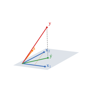
This is also why all the Z-scores of a group of highly correlated inputs can be small: any one of them can be removed (the others carry the information), but not all of them.
Result 3.9 (the QR decomposition and the least-squares fit) p. 55, (3.30)–(3.33); Exercise 3.4
Step 2 of Algorithm 3.1 is the matrix factorisation
\[ \bX=\bZ\mathbf{\Gamma}, \tag{3.30} \]with \(\bZ=(\bz_0,\dots,\bz_p)\) and \(\mathbf{\Gamma}\) unit upper triangular (entries \(\hat\gamma_{kj}\)). With \(\bD=\diag(\|\bz_j\|)\),
\[ \bX=\bZ\bD^{-1}\bD\mathbf{\Gamma}=\bQ\bR, \tag{3.31} \]\(\bQ^\T\bQ=\bI\), \(\bR\) upper triangular, and
\[ \hb=\bR^{-1}\bQ^\T\by, \tag{3.32} \] \[ \hat\by=\bQ\bQ^\T\by. \tag{3.33} \]One pass of Gram–Schmidt thus gives every coefficient: compute \(\bQ^\T\by\) and solve the triangular system \(\bR\hb=\bQ^\T\by\) by back-substitution.
Proof
(3.30) is the rearranged step 2, \(\bx_j=\bz_j+\sum_{k\lt j}\hat\gamma_{kj}\bz_k\), written column by column. Inserting \(\bD^{-1}\bD=\bI\) gives \(\bQ=\bZ\bD^{-1}\), whose columns are the orthonormal \(\bz_j/\|\bz_j\|\), and \(\bR=\bD\mathbf{\Gamma}\), upper triangular with positive diagonal. Then \(\bX^\T\bX=\bR^\T\bQ^\T\bQ\bR=\bR^\T\bR\) and \(\bX^\T\by=\bR^\T\bQ^\T\by\); the normal equations become \(\bR^\T\bR\hb=\bR^\T\bQ^\T\by\), and \(\bR^\T\) is invertible, so \(\bR\hb=\bQ^\T\by\): (3.32). Then \(\hat\by=\bQ\bR\hb=\bQ\bQ^\T\by\): (3.33). Back-substitution solves \(\bR\hb=\bQ^\T\by\) from the last coefficient upwards: \(\hat\beta_p=(\bQ^\T\by)_p/R_{pp}\), which is (3.28), then \(\hat\beta_j=\big((\bQ^\T\by)_j-\sum_{k>j}R_{jk}\hat\beta_k\big)/R_{jj}\). ∎
See also (companion course): conditioning and why one avoids forming \(\bX^\T\bX\); Section 3.9 below.
3.2.4 Multiple Outputs
p. 56 With \(K\) outputs, a linear model for each,
\[ Y_k=\beta_{0k}+\sum_{j=1}^pX_j\beta_{jk}+\varepsilon_k \tag{3.34} \] \[ =f_k(X)+\varepsilon_k, \tag{3.35} \]in matrix form \(\bY=\bX\bB+\mathbf{E}\), with \(\bY\) of size \(N\times K\) and \(\bB\) of size \((p+1)\times K\):
\[ \bY=\bX\bB+\mathbf{E}. \tag{3.36} \]The sum of the \(K\) residual sums of squares,
\[ \RSS(\bB)=\sum_{k=1}^K\sum_{i=1}^N\big(y_{ik}-f_k(x_i)\big)^2 \tag{3.37} \] \[ =\tr\big[(\bY-\bX\bB)^\T(\bY-\bX\bB)\big], \tag{3.38} \]is minimised column by column, giving
\[ \hat\bB=(\bX^\T\bX)^{-1}\bX^\T\bY. \tag{3.39} \]If the errors of one case are correlated, \(\Cov(\varepsilon)=\mathbf{\Sigma}\), the Gaussian likelihood suggests the weighted criterion
\[ \RSS(\bB;\mathbf{\Sigma})=\sum_{i=1}^N\big(y_i-f(x_i)\big)^\T\mathbf{\Sigma}^{-1}\big(y_i-f(x_i)\big). \tag{3.40} \]Result 3.10 (multiple outputs decouple; Exercise 3.11) p. 56
For any positive definite \(\mathbf{\Sigma}\) the minimiser of (3.40) is (3.39). If the covariance \(\mathbf{\Sigma}_i\) varies with the case, it is not in general.
Proof
(3.40) equals \(\tr\big[(\bY-\bX\bB)\mathbf{\Sigma}^{-1}(\bY-\bX\bB)^\T\big]\). Its gradient in \(\bB\) is \(-2\bX^\T(\bY-\bX\bB)\mathbf{\Sigma}^{-1}\); setting it to zero and multiplying on the right by \(\mathbf{\Sigma}\) gives \(\bX^\T(\bY-\bX\bB)=\mathbf{0}\), the \(K\) separate normal equations, whose solution is (3.39). Convexity (the Hessian is \(2\mathbf{\Sigma}^{-1}\otimes\bX^\T\bX\succ0\)) makes it the minimiser. With case-dependent \(\mathbf{\Sigma}_i\) the stationarity condition is \(\sum_ix_i(y_i-\bB^\T x_i)^\T\mathbf{\Sigma}_i^{-1}=\mathbf{0}\), which cannot be multiplied through by a single matrix; the solution mixes the columns (a numerical example in the code changes \(\hat\bB\) visibly). The companion courses prove the same: Result 4.8. ∎
3.3 Subset Selection
p. 57 Least squares is often unsatisfactory for two reasons: prediction accuracy (low bias but high variance, which shrinking or deleting coefficients can reduce) and interpretation (a small subset with the strongest effects is easier to understand). Subset selection keeps some inputs, fits them by least squares, and drops the rest.
3.3.1 Best-Subset Selection
pp. 57–58 For each size \(k\in\{0,1,\dots,p\}\), best-subset regression finds the subset of \(k\) inputs with the smallest RSS. The leaps-and-bounds algorithm (Furnival and Wilson, 1974) avoids most of the \(2^p\) fits by bounding: adding variables never increases the RSS, so a large subset whose RSS is already worse than the best \(k\)-subset found rules out all of its \(k\)-subsets. This makes \(p\) up to 30 or 40 feasible (the code uses it, through R's leaps, for the 31 inputs of Figure 3.6, and checks it against the exhaustive search on the prostate data).
The best RSS is non-increasing in \(k\): the best \(k\)-subset plus any other input is a \((k+1)\)-subset with no larger RSS, because the larger column space contains the smaller (Result 3.2). So the training RSS cannot choose \(k\); that needs an estimate of prediction error (cross-validation, AIC; Chapter 7).
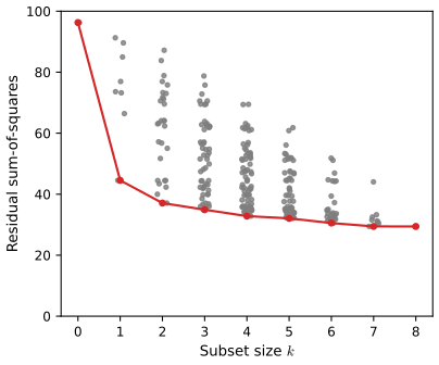
3.3.2 Forward- and Backward-Stepwise Selection
pp. 58–60 Forward stepwise starts from the intercept and repeatedly adds the input that most reduces the RSS; it is greedy and gives a nested sequence, but it is cheap (it works even when \(p\gg N\)) and, being a more constrained search, has lower variance than best subset. Backward stepwise starts from the full model (so needs \(N>p\)) and repeatedly drops the input whose removal increases the RSS least. Both rely on two updating formulas.
Result 3.11 (fast forward step; Exercise 3.9) p. 58
Let the current model have columns \(\bX_1\) with thin QR factor \(\bQ\) (orthonormal basis of \(\col(\bX_1)\)) and residual \(\br=\by-\bQ\bQ^\T\by\). For a candidate column \(\bx_j\), put \(\bz_j=\bx_j-\bQ\bQ^\T\bx_j\). Adding \(\bx_j\) reduces the RSS by exactly
\[ \Delta_j=\frac{\langle\br,\bz_j\rangle^2}{\|\bz_j\|^2}=\|\br\|^2\,\Corr^2(\br,\bz_j)\ \text{(for centred vectors)}, \]so the best candidate maximises \(|\langle\br,\bz_j\rangle|/\|\bz_j\|\); the QR factor is then updated by one Gram–Schmidt step, \(\bQ\leftarrow(\bQ,\bz_j/\|\bz_j\|)\), at cost \(O(Nq)\) per candidate instead of a new fit.
Proof
\(\col(\bX_1,\bx_j)=\col(\bQ,\bz_j)\) and \(\bz_j\perp\col(\bQ)\), so the new projection is \(\bQ\bQ^\T+\bz_j\bz_j^\T/\|\bz_j\|^2\) and the new residual is \(\br-\bz_j\langle\bz_j,\by\rangle/\|\bz_j\|^2\). Since \(\bz_j\perp\bQ\), \(\langle\bz_j,\by\rangle=\langle\bz_j,\br\rangle\). The removed part is orthogonal to the new residual, so by Pythagoras the RSS falls by \(\langle\br,\bz_j\rangle^2/\|\bz_j\|^2\). (Confirmed numerically against refitting.) ∎
Result 3.12 (backward step drops the smallest |Z|; Exercise 3.10) p. 59
Dropping \(\bx_j\) from the full fit increases the RSS by \(\hat\beta_j^2/v_j=z_j^2\hat\sigma^2\). Hence the variable whose removal hurts least is the one with the smallest \(|z_j|\), and it can be read off Table 3.2 without refitting.
Proof
This is the identity \(\RSS_0-\RSS_1=\hat\beta_j^2/v_j\) proved in Filling the gap 3.2(c), with \(\hat\sigma^2\) the same for every \(j\). ∎
On the prostate data best-subset, forward and backward selection give exactly the same sequence of models (confirmed by the code). Hybrid procedures (R's step) consider adds and drops at each step and score them by AIC; procedures based on F-tests ignore the multiple testing, and the standard errors printed for a model chosen by a search are not valid because they ignore the search (the bootstrap of Section 8.2 can help). Groups of dummy variables should enter and leave together.
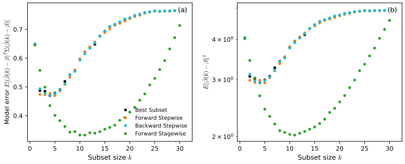
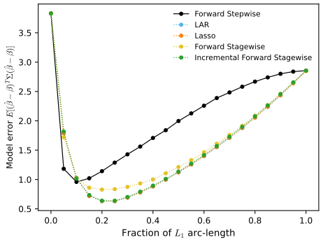
Note on Figure 3.6: what the vertical axis can be
The book labels the axis \(\E\|\hat\bb(k)-\bb\|^2\) and its curves end at about 0.66 for the full model. That cannot be the squared coefficient error under the stated design: for least squares on all 31 inputs, \[ \E\|\hat\bb-\bb\|^2=\sigma^2\,\E\tr(\bX^\T\bX)^{-1}=\sigma^2\tr(\mathbf{\Sigma}^{-1})/(N-p-1)=6.25\times200.04/268=4.67 \] (our simulation: 4.92, panel (b)). The model error at the full model is \(\sigma^2p/(N-p-1)=0.72\) (simulation: 0.77, panel (a)), the right order of magnitude, so the book most likely plotted a prediction-type error. Even then the shapes differ: under the stated design both quantities rise again for large \(k\) (variance grows with every useless input), whereas the book's curves stay flat from \(k\approx15\) to 31, and forward stagewise does better, not worse, than the subset methods at intermediate sizes because its coefficients are shrunk. What does reproduce is the book's main point: best subset, forward and backward stepwise perform almost identically.
3.3.3 Forward-Stagewise Regression
p. 60 Forward-stagewise regression (FS) is even more constrained. With centred inputs and the intercept \(\bar y\), it starts from all coefficients zero; at each step it finds the input most correlated with the current residual, computes the simple regression coefficient of the residual on that input, and adds it to that input's coefficient; nothing else is adjusted. It stops when no input is correlated with the residual, which for \(N>p\) is the least-squares fit (a stationary point has \(\bX^\T\br=\mathbf{0}\), the normal equations). It can take many more than \(p\) steps (over a thousand in Figure 3.6), which is exactly why it is a slow, heavily regularised fitting procedure, and it reappears as the linear version of boosting (Section 3.8.1, Chapter 10).
3.3.4 Prostate Cancer Data Example (Continued)
pp. 61–63 Table 3.3 compares the methods, each with its complexity chosen by tenfold cross-validation on the 67 training cases and the one-standard-error rule: take the least complex model whose CV error is within one standard error of the minimum (the standard error is the standard deviation of the ten fold errors over \(\sqrt{10}\); Section 7.10). The test set is used only to judge the chosen models.
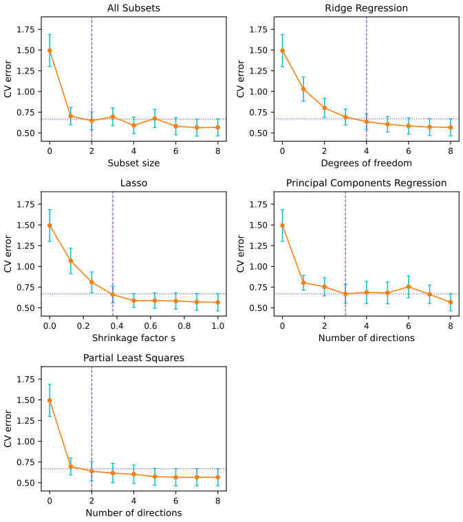
Table 3.3. Coefficients and test error at the book's chosen complexities p. 63
| Term | LS | Best subset | Ridge | Lasso | PCR | PLS |
|---|---|---|---|---|---|---|
| Intercept | 2.465 | 2.477 | 2.464 | 2.469 | 2.497 | 2.467 |
| lcavol | 0.680 | 0.740 | 0.421 | 0.533 | 0.551 | 0.419 |
| lweight | 0.263 | 0.316 | 0.239 | 0.176 | 0.289 | 0.345 |
| age | −0.141 | −0.048 | −0.155 | −0.026 | ||
| lbph | 0.210 | 0.162 | 0.214 | 0.220 | ||
| svi | 0.305 | 0.227 | 0.074 | 0.315 | 0.243 | |
| lcp | −0.288 | 0.000 | −0.062 | 0.078 | ||
| gleason | −0.021 | 0.041 | 0.228 | 0.011 | ||
| pgg45 | 0.267 | 0.132 | −0.048 | 0.084 | ||
| Test error | 0.521 | 0.492 | 0.490 | 0.490 | 0.449 | 0.527 |
| Std error | 0.179 | 0.143 | 0.162 | 0.169 | 0.106 | 0.150 |
Fitted at the book's choices: best subset {lcavol, lweight}, ridge df = 5 (\(\lambda=24.00\)), lasso \(s=0.36\), PCR with 7 and PLS with 2 directions. The LS and best-subset columns equal the book's to every printed digit; ridge and PLS agree to 0.002 and PCR to 0.012 in the coefficients. Three differences are explained in the notes on the book: the book's ridge and PLS intercepts (2.452) and hence their test errors, and its lasso column. Reproduces Hastie, Tibshirani and Friedman (2009), Table 3.3.
Best subset picks {lcavol, lweight}; PCR gives the lowest test error, but all the test errors are within about one standard error of each other (the test set has only 30 cases).
3.4 Shrinkage Methods
p. 61 Subset selection is a discrete process (an input is in or out), so a small change in the data can change the model, which gives high variance. Shrinkage methods are continuous and vary less.
3.4.1 Ridge Regression
pp. 61–68 Ridge regression penalises the size of the coefficients:
\[ \hb^{\rm ridge}=\argmin_{\bb}\Big\{\sum_{i=1}^N\Big(y_i-\beta_0-\sum_{j=1}^px_{ij}\beta_j\Big)^2+\lambda\sum_{j=1}^p\beta_j^2\Big\}, \tag{3.41} \]or equivalently, as a constrained problem,
\[ \hb^{\rm ridge}=\argmin_{\bb}\sum_{i=1}^N\Big(y_i-\beta_0-\sum_{j=1}^px_{ij}\beta_j\Big)^2\ \ \text{subject to}\ \sum_{j=1}^p\beta_j^2\le t. \tag{3.42} \]The penalty tames the wildly large, mutually cancelling coefficients of correlated inputs. It is not equivariant under rescaling of the inputs, so they are standardised first, and the intercept is not penalised (penalising it would make the fit depend on the origin of \(Y\)). After centring (Exercise 3.5, Result 3.13(a)), \(\hat\beta_0=\bar y\) and the rest solve a ridge problem without intercept; from now on \(\bX\) is the \(N\times p\) matrix of centred inputs and \(\by\) is centred:
\[ \RSS(\lambda)=(\by-\bX\bb)^\T(\by-\bX\bb)+\lambda\bb^\T\bb, \tag{3.43} \] \[ \hb^{\rm ridge}=(\bX^\T\bX+\lambda\bI)^{-1}\bX^\T\by. \tag{3.44} \]Adding \(\lambda>0\) to the diagonal makes the system nonsingular even when \(\bX^\T\bX\) is not, which was the original motivation (Hoerl and Kennard, 1970). With orthonormal inputs, \(\hb^{\rm ridge}=\hb/(1+\lambda)\).
The SVD of the centred input matrix,
\[ \bX=\bU\bD\bV^\T, \tag{3.45} \]has \(\bU\) (\(N\times p\)) and \(\bV\) (\(p\times p\)) with orthonormal columns and \(\bD=\diag(d_1\ge\dots\ge d_p\ge0)\). It gives
\[ \bX\hb^{\rm ls}=\bX(\bX^\T\bX)^{-1}\bX^\T\by=\bU\bU^\T\by, \tag{3.46} \] \[ \bX\hb^{\rm ridge}=\bX(\bX^\T\bX+\lambda\bI)^{-1}\bX^\T\by=\bU\bD(\bD^2+\lambda\bI)^{-1}\bD\bU^\T\by=\sum_{j=1}^p\bu_j\frac{d_j^2}{d_j^2+\lambda}\bu_j^\T\by, \tag{3.47} \] \[ \bX^\T\bX=\bV\bD^2\bV^\T, \tag{3.48} \] \[ \Var(\bz_1)=\Var(\bX\bv_1)=\frac{d_1^2}{N}, \tag{3.49} \] \[ \df(\lambda)=\tr\big[\bX(\bX^\T\bX+\lambda\bI)^{-1}\bX^\T\big]=\tr(\bH_\lambda)=\sum_{j=1}^p\frac{d_j^2}{d_j^2+\lambda}. \tag{3.50} \]Result 3.13 (ridge regression: intercept, SVD form, principal components, degrees of freedom) pp. 63–68; Exercises 3.5, 3.12
(a) The solution of (3.41) has \(\hat\beta_0=\bar y-\sum_j\bar x_j\hat\beta_j\), and \((\hat\beta_1,\dots,\hat\beta_p)\) is (3.44) computed from the centred inputs; equivalently (3.85) with \(\beta^c_0=\bar y\). (b) (3.46)–(3.47) hold: ridge computes the coordinates \(\bu_j^\T\by\) of \(\by\) in the basis \(\bU\) and shrinks them by \(d_j^2/(d_j^2+\lambda)\le1\), most for small \(d_j\). (c) \(\bv_j\) are the principal component directions: \(\bz_j=\bX\bv_j=d_j\bu_j\) has sample variance \(d_j^2/N\), the largest possible among unit directions orthogonal to \(\bv_1,\dots,\bv_{j-1}\). (d) \(\df(\lambda)\) in (3.50) decreases strictly from \(\rank\bX\) at \(\lambda=0\) to 0 as \(\lambda\to\infty\). (e) Ridge is least squares on the data augmented with the \(p\) rows \(\sqrt\lambda\bI\) and \(p\) zero responses.
Filling the gap 3.6: the ridge identities "after some simplification" pp. 64–68
Derivation
(a) Centring. Write \(\beta_0+\sum_jx_{ij}\beta_j=\beta_0^c+\sum_j(x_{ij}-\bar x_j)\beta_j\) with \(\beta^c_0=\beta_0+\sum_j\bar x_j\beta_j\): a one-to-one reparametrisation that leaves the slopes and the penalty unchanged. In the new parameters the derivative in \(\beta^c_0\) is \[ -2\sum_i\big(y_i-\beta^c_0-\sum_j(x_{ij}-\bar x_j)\beta_j\big)=-2N(\bar y-\beta^c_0) \] since the centred inputs sum to zero; so \(\hat\beta^c_0=\bar y\) whatever the slopes, and the slopes minimise the ridge criterion with centred inputs and response \(y_i-\bar y\), which is (3.43) with solution (3.44) (the Hessian \(2(\bX^\T\bX+\lambda\bI)\) is positive definite). Undoing the reparametrisation gives \(\hat\beta_0\). The lasso argument is identical with \(|\beta_j|\) in place of \(\beta_j^2\).
(b) SVD form. With \(\bX=\bU\bD\bV^\T\), \(\bX^\T\bX=\bV\bD^2\bV^\T\) (this is (3.48)) and, \(\bV\) being square orthogonal, \(\bX^\T\bX+\lambda\bI=\bV(\bD^2+\lambda\bI)\bV^\T\), whose inverse is \(\bV(\bD^2+\lambda\bI)^{-1}\bV^\T\). Hence \[ \bX(\bX^\T\bX+\lambda\bI)^{-1}\bX^\T=\bU\bD\bV^\T\bV(\bD^2+\lambda\bI)^{-1}\bV^\T\bV\bD\bU^\T=\bU\bD(\bD^2+\lambda\bI)^{-1}\bD\bU^\T \], a sum of rank-one terms \(\frac{d_j^2}{d_j^2+\lambda}\bu_j\bu_j^\T\): (3.47). At \(\lambda=0\) (full rank) the factors are 1: (3.46). The coefficients are \(\hb^{\rm ridge}=\sum_j\bv_j\frac{d_j}{d_j^2+\lambda}\bu_j^\T\by\).
(c) Principal components. For a unit vector \(\ba\), the sample variance of the centred \(\bX\ba\) is \[ \|\bX\ba\|^2/N=\ba^\T\bV\bD^2\bV^\T\ba/N=\sum_jd_j^2c_j^2/N \] with \(\mathbf{c}=\bV^\T\ba\), \(\|\mathbf{c}\|=1\). This is at most \(d_1^2/N\), attained at \(\mathbf{c}=e_1\), i.e. \(\ba=\bv_1\): (3.49), and \(\bX\bv_1=\bU\bD\bV^\T\bv_1=d_1\bu_1\). Requiring \(\ba\perp\bv_1,\dots,\bv_{j-1}\) forces \(c_1=\dots=c_{j-1}=0\) and the maximum becomes \(d_j^2/N\). Small \(d_j\) are directions in which the inputs barely vary, where the slope of the fitted plane is poorly determined; ridge shrinks those coordinates most (Figure 3.9).
(d) Degrees of freedom. \[ \tr(\bH_\lambda)=\tr\big(\bD(\bD^2+\lambda\bI)^{-1}\bD\bU^\T\bU\big)=\sum_jd_j^2/(d_j^2+\lambda) \], using \(\bU^\T\bU=\bI\). Each term with \(d_j>0\) has derivative \(-d_j^2/(d_j^2+\lambda)^2\lt 0\), equals 1 at \(\lambda=0\) and tends to 0; terms with \(d_j=0\) vanish. (The covariance definition (3.60) gives the same number: Result 3.20.)
(e) Augmented data. With \(\tilde\bX=\binom{\bX}{\sqrt\lambda\bI}\), \(\tilde\by=\binom{\by}{\mathbf{0}}\): \(\tilde\bX^\T\tilde\bX=\bX^\T\bX+\lambda\bI\) and \(\tilde\bX^\T\tilde\by=\bX^\T\by\), so ordinary least squares on the augmented data is (3.44). The artificial cases "pull" each coefficient towards 0. ∎
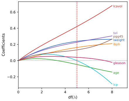
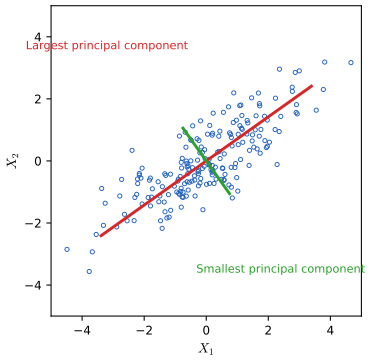
The implicit assumption is that the response varies most along the high-variance directions of the inputs; it is often reasonable (inputs are chosen because they relate to the response) but need not hold.
See also (companion courses): ridge through the SVD; weight decay and the effective number of parameters; the effective number of parameters \(\gamma\), which is \(\df(\lambda)\) with the Bayesian choice of \(\lambda\).
Result 3.14 (penalised and constrained forms are equivalent) p. 63, (3.41)–(3.42), and p. 68, (3.51)–(3.52)
Let \(J(\bb)\) be \(\|\bb\|^2\) or \(\|\bb\|_1\). For every \(\lambda\ge0\), a minimiser of \(\RSS(\bb)+\lambda J(\bb)\) solves the constrained problem with \(t=J(\hb_\lambda)\). Conversely, for every \(t\) with \(0\lt t\lt J(\hb^{\rm ls})\) (minimum-\(J\) least-squares solution) there is a \(\lambda>0\) such that the constrained solutions are penalised solutions. For ridge with \(\bX\) of full rank the correspondence \(\lambda\leftrightarrow t\) is one-to-one and decreasing.
Proof
(\(\Rightarrow\)) If \(\hb_\lambda\) minimises \(\RSS+\lambda J\) and \(J(\bb)\le t=J(\hb_\lambda)\), then \[ \RSS(\bb)\ge\RSS(\hb_\lambda)+\lambda(J(\hb_\lambda)-J(\bb))\ge\RSS(\hb_\lambda) \]. (\(\Leftarrow\)) The constrained problem is convex, and \(\bb=\mathbf{0}\) is strictly feasible when \(t>0\) (Slater's condition), so strong duality holds and a Lagrange multiplier \(\lambda\ge0\) exists with the constrained solution minimising \(\RSS+\lambda(J-t)\); if \(t\lt J(\hb^{\rm ls})\) the constraint is active and \(\lambda>0\). For ridge with full rank, \(\|\hb_\lambda\|^2=\sum_jd_j^2(\bu_j^\T\by)^2/(d_j^2+\lambda)^2\) is strictly decreasing in \(\lambda\) (unless \(\bX^\T\by=\mathbf{0}\)), so \(t(\lambda)\) is a bijection from \((0,\infty)\) onto \((0,\|\hb^{\rm ls}\|^2)\). Full details, with the geometry: Foundations of Deep Learning, Result 9.6; Bayesian and Probabilistic ML, Result 3.6. ∎
Result 3.15 (ridge as a posterior mean and mode; Exercises 3.6–3.7) p. 64
If \(y_i\sim\N(\beta_0+x_i^\T\bb,\sigma^2)\) independently and \(\beta_j\sim\N(0,\tau^2)\) independently, with \(\sigma^2,\tau^2\) known (and a flat prior on \(\beta_0\)), then minus twice \(\sigma^2\) times the log-posterior of \(\bb\) is, up to a constant, the bracket in (3.41) with \(\lambda=\sigma^2/\tau^2\). The posterior is Gaussian, so its mode and mean coincide and equal \(\hb^{\rm ridge}\).
Proof
The log-likelihood is \(-\frac{1}{2\sigma^2}\sum_i(y_i-\beta_0-x_i^\T\bb)^2+\)const and the log-prior \(-\frac{1}{2\tau^2}\sum_j\beta_j^2+\)const. Their sum times \(-2\sigma^2\) is \(\sum_i(y_i-\beta_0-x_i^\T\bb)^2+\frac{\sigma^2}{\tau^2}\sum_j\beta_j^2\)+const. As a function of \((\beta_0,\bb)\) the log-posterior is a concave quadratic, so the posterior is Gaussian; for a Gaussian the mean is the mode, which minimises the expression above: ridge with \(\lambda=\sigma^2/\tau^2\). Explicitly (centred data) the posterior is \[ \N\big((\bX^\T\bX+\lambda\bI)^{-1}\bX^\T\by,\ \sigma^2(\bX^\T\bX+\lambda\bI)^{-1}\big) \], by completing the square. The companion course derives the same posterior in Bishop's notation: Result 3.11. ∎
3.4.2 The Lasso
pp. 68–69 The lasso (Tibshirani, 1996; "basis pursuit" in signal processing, Chen et al., 1998) replaces the \(L_2\) penalty by the \(L_1\) penalty:
\[ \hb^{\rm lasso}=\argmin_{\bb}\sum_{i=1}^N\Big(y_i-\beta_0-\sum_{j=1}^px_{ij}\beta_j\Big)^2\ \ \text{subject to}\ \sum_{j=1}^p|\beta_j|\le t, \tag{3.51} \] \[ \hb^{\rm lasso}=\argmin_{\bb}\Big\{\frac12\sum_{i=1}^N\Big(y_i-\beta_0-\sum_{j=1}^px_{ij}\beta_j\Big)^2+\lambda\sum_{j=1}^p|\beta_j|\Big\}. \tag{3.52} \]As for ridge, \(\hat\beta_0=\bar y\) after centring. The solution is nonlinear in \(\by\) and has no closed form; it is a quadratic programme, but its whole path can be computed by least angle regression (Section 3.4.4). If \(t\ge t_0=\sum_j|\hat\beta^{\rm ls}_j|\) the lasso is least squares; smaller \(t\) sets some coefficients exactly to zero, a continuous form of subset selection.
Result 3.16 (optimality conditions of the lasso) pp. 68, 76–77, (3.58)–(3.59); Exercise 3.27
For centred data and \(\lambda>0\), \(\hb\) minimises \(R(\bb)=\frac12\|\by-\bX\bb\|^2+\lambda\|\bb\|_1\) if and only if, with \(\br=\by-\bX\hb\),
\[ \bx_j^\T\br=\lambda\,\sign(\hat\beta_j)\ \text{ if }\hat\beta_j\ne0,\qquad |\bx_j^\T\br|\le\lambda\ \text{ if }\hat\beta_j=0. \]Moreover: a minimiser exists; all minimisers have the same fitted vector \(\bX\hb\) and the same \(L_1\) norm; \(\hb=\mathbf{0}\) iff \(\lambda\ge\lambda_{\max}=\max_j|\bx_j^\T\by|\); the minimiser is unique when the columns of \(\bX\) are in general position (in particular with probability one for continuous inputs).
Filling the gap 3.7: subgradients and the lasso's optimality conditions pp. 76–77
Derivation
Convex optimality. \(R\) is convex; \(\hb\) minimises it iff \(\mathbf{0}\in\partial R(\hb)\), the subdifferential. The quadratic part is differentiable with gradient \(-\bX^\T\br\). The subdifferential of \(|\beta|\) is \(\{\sign\beta\}\) for \(\beta\ne0\) and \([-1,1]\) at 0 (the slopes of all lines through the origin lying below \(|\cdot|\)). As \(\|\bb\|_1\) is a separable sum, \[ \partial R(\hb)=\{-\bX^\T\br+\lambda\bs:\ s_j=\sign\hat\beta_j\text{ if }\hat\beta_j\ne0,\ s_j\in[-1,1]\text{ otherwise}\} \]. Zero belongs to it exactly under the stated conditions. (Elementary check without subgradients: for \(\hat\beta_j=0\), the one-sided derivatives of \(R\) along \(\pm e_j\) are \(\mp\bx_j^\T\br+\lambda\), both \(\ge0\) iff \(|\bx_j^\T\br|\le\lambda\).)
The KKT form of Exercise 3.27. Writing \(\beta_j=\beta_j^+-\beta_j^-\) with \(\beta_j^\pm\ge0\) turns (3.52) into a smooth problem with non-negativity constraints, and the KKT conditions with multipliers \(\lambda_j^\pm\ge0\) are exactly the conditions above; see the solution of Exercise 3.27.
Existence. \(R\) is continuous and \(R(\bb)\ge\lambda\|\bb\|_1\to\infty\) as \(\|\bb\|\to\infty\) (coercive), so a minimiser exists.
Uniqueness of the fit. If \(\hb,\tilde\bb\) are both minimisers with \(\bX\hb\ne\bX\tilde\bb\), the midpoint has strictly smaller quadratic part (\(\|\cdot\|^2\) is strictly convex) and no larger penalty, a contradiction. So the fit, hence \(\br\) and \(R\), are common to all minimisers, and then \(\lambda\|\bb\|_1=R-\frac12\|\br\|^2\) is common too.
\(\lambda_{\max}\). \(\hb=\mathbf{0}\) gives \(\br=\by\), and the conditions reduce to \(|\bx_j^\T\by|\le\lambda\) for all \(j\).
Uniqueness of \(\hb\). Let \(E=\{j:|\bx_j^\T\br|=\lambda\}\) (common to all solutions, since \(\br\) is). Every solution vanishes off \(E\) and satisfies \(\bX_E\bb_E=\bX\hb\). If the columns \(\bX_E\) are linearly independent, \(\bb_E\) is determined. General position (no \(k+1\) of the signed columns \(\pm\bx_j\) lie in a \((k-1)\)-dimensional affine subspace) guarantees this (Tibshirani, 2013). ∎
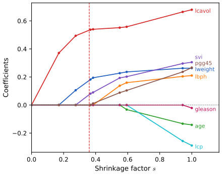
3.4.3 Discussion: Subset Selection, Ridge Regression and the Lasso
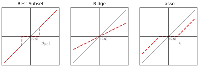
pp. 69–73 With orthonormal inputs the three methods have explicit solutions (Table 3.4): best subset of size \(M\) keeps the \(M\) largest coefficients (hard thresholding), ridge scales them proportionally, and the lasso translates each towards zero by \(\lambda\), truncating at zero (soft thresholding, used for wavelets in Section 5.9).
Table 3.4. Estimators of \(\beta_j\) when \(\bX\) has orthonormal columns p. 71
| Estimator | Formula |
|---|---|
| Best subset (size \(M\)) | \(\hat\beta_j\cdot I\big(|\hat\beta_j|\ge|\hat\beta_{(M)}|\big)\) |
| Ridge | \(\hat\beta_j/(1+\lambda)\) |
| Lasso | \(\sign(\hat\beta_j)(|\hat\beta_j|-\lambda)_+\) |
Result 3.17 (the entries of Table 3.4; Exercise 3.16) p. 71
If \(\bX^\T\bX=\bI\) and \(\hat\beta_j=\bx_j^\T\by\), then best subset of size \(M\), ridge (3.41) and the lasso (3.52) are given by Table 3.4.
Proof
For any \(\bb\), \[ \|\by-\bX\bb\|^2=\|\by-\bX\hb\|^2+\|\bX(\hb-\bb)\|^2=\RSS_{\rm ls}+\sum_j(\hat\beta_j-\beta_j)^2 \] (Pythagoras and \(\bX^\T\bX=\bI\)). So every criterion separates into one-dimensional problems. Subset: keeping set \(S\) with least-squares values gives \(\RSS_{\rm ls}+\sum_{j\notin S}\hat\beta_j^2\), minimised over \(|S|=M\) by keeping the \(M\) largest \(|\hat\beta_j|\). Ridge: \((\hat\beta_j-\beta)^2+\lambda\beta^2\) has derivative \(-2(\hat\beta_j-\beta)+2\lambda\beta=0\) at \(\beta=\hat\beta_j/(1+\lambda)\). Lasso: \(\frac12(\hat\beta_j-\beta)^2+\lambda|\beta|\); for \(\beta>0\) the derivative vanishes at \(\beta=\hat\beta_j-\lambda\), admissible iff \(\hat\beta_j>\lambda\); for \(\beta\lt 0\), at \(\hat\beta_j+\lambda\lt 0\); otherwise the subgradient condition \(|\hat\beta_j|\le\lambda\) makes 0 optimal. Together: \(\sign(\hat\beta_j)(|\hat\beta_j|-\lambda)_+\). (With the book's (3.52) the threshold is \(\lambda\); without the factor \(\frac12\) it would be \(\lambda/2\).) ∎
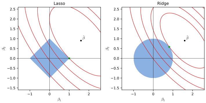
See also (companion courses): why the lasso gives exact zeros and \(q>1\) never does; the lasso picture; the L1 versus L2 demo (simulated data, any \(q\)).
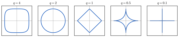
More generally, consider the \(L_q\) criterion
\[ \tilde\bb=\argmin_{\bb}\Big\{\sum_{i=1}^N\Big(y_i-\beta_0-\sum_{j=1}^px_{ij}\beta_j\Big)^2+\lambda\sum_{j=1}^p|\beta_j|^q\Big\}, \tag{3.53} \]for \(q\ge0\): \(q=0\) counts nonzero coefficients (subset selection), \(q=1\) is the lasso, \(q=2\) ridge. Viewing \(|\beta_j|^q\) as a log-prior, (3.53) is a posterior mode; for \(q=1\) the prior is the Laplace (double-exponential) density \(\frac{1}{2\tau}e^{-|\beta|/\tau}\). The lasso is the smallest \(q\) with a convex constraint region.
Filling the gap 3.8: the Bayesian reading of (3.53), and posterior mode versus mean p. 72
Derivation
With Gaussian errors of variance \(\sigma^2\) and independent priors \(p(\beta_j)\propto e^{-|\beta_j|^q/\kappa}\), minus \(2\sigma^2\) times the log-posterior is \(\RSS(\bb)+\frac{2\sigma^2}{\kappa}\sum_j|\beta_j|^q\)+const, so the mode solves (3.53) with \(\lambda=2\sigma^2/\kappa\). For \(q=1\) and the Laplace prior \(\frac{1}{2\tau}e^{-|\beta|/\tau}\) (\(\kappa=\tau\)) this gives \(\lambda=2\sigma^2/\tau\) for (3.53), or \(\lambda=\sigma^2/\tau\) for the halved criterion (3.52). The book's "\(\tau=1/\lambda\)" is the special case \(\sigma^2=\frac12\) of (3.53) (or \(\sigma^2=1\) of (3.52)): the scale of the noise matters.
Mode is not mean. For ridge the posterior is Gaussian, so mode = mean (Result 3.15). For the Laplace prior, take one orthonormal input: the posterior of \(\beta\) is proportional to \(\exp\{-(\beta-\hat\beta)^2/(2\sigma^2)-|\beta|/\tau\}\), a density with no atom at 0, so its mean is never exactly 0 (it is a smooth, strictly increasing function of \(\hat\beta\)), while its mode is the soft-thresholded value, exactly 0 for \(|\hat\beta|\le\sigma^2/\tau\). The lasso's exact zeros are a property of the mode only. ∎
See also (companion course): other priors; the lasso as a MAP estimate.
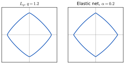
p. 73 Values \(q\in(1,2)\) compromise between lasso and ridge, but for \(q>1\) the penalty \(|\beta|^q\) is differentiable at 0, so it never sets coefficients exactly to zero (the one-dimensional optimality condition \(\beta-\hat\beta+\frac{\lambda q}{2}|\beta|^{q-1}\sign\beta=0\) has \(\beta=0\) as a solution only if \(\hat\beta=0\)). Zou and Hastie (2005) proposed instead the elastic net penalty
\[ \lambda\sum_{j=1}^p\big(\alpha\beta_j^2+(1-\alpha)|\beta_j|\big), \tag{3.54} \]which selects like the lasso (its \(L_1\) part has a corner at 0) and shrinks correlated inputs together like ridge (its \(L_2\) part is strictly convex: two identical inputs get identical coefficients, see Exercises 3.28–3.29). Exercise 3.30 turns it into a lasso on augmented data.
3.4.4 Least Angle Regression
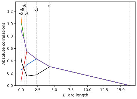
pp. 73–79 Least angle regression (LAR; Efron et al., 2004) is a "democratic" forward stepwise method: rather than fitting an entering variable completely, it moves its coefficient only until another variable is equally correlated with the residual, and then moves them together.
Algorithm 3.2 (least angle regression) p. 74
- Standardise the predictors to mean zero and unit norm. Start with \(\br=\by-\bar y\bone\) and \(\beta_1=\dots=\beta_p=0\).
- Find the predictor \(\bx_j\) most correlated with \(\br\).
- Move \(\beta_j\) from 0 towards its least-squares coefficient \(\langle\bx_j,\br\rangle\) until some other \(\bx_k\) has as much correlation with the current residual as \(\bx_j\).
- Move \(\beta_j\) and \(\beta_k\) in the direction of their joint least-squares coefficient of the current residual on \((\bx_j,\bx_k)\), until some other \(\bx_l\) has as much correlation with the current residual.
- Continue until all \(p\) predictors have entered. After \(\min(N-1,p)\) steps, this is the full least-squares solution.
If \(\mathcal{A}_k\) is the active set at the start of step \(k\), \(\bb_{\mathcal{A}_k}\) its coefficients and \(\br_k=\by-\bX_{\mathcal{A}_k}\bb_{\mathcal{A}_k}\), the direction of step \(k\) is
\[ \bd_k=(\bX_{\mathcal{A}_k}^\T\bX_{\mathcal{A}_k})^{-1}\bX_{\mathcal{A}_k}^\T\br_k, \tag{3.55} \]and the coefficients move as \(\bb_{\mathcal{A}_k}(\alpha)=\bb_{\mathcal{A}_k}+\alpha\bd_k\), the fit as \(\hat{\mathbf{f}}_k(\alpha)=\hat{\mathbf{f}}_k+\alpha\bu_k\) with \(\bu_k=\bX_{\mathcal{A}_k}\bd_k\).
Result 3.18 (what a LAR step does; Exercises 3.23–3.25) pp. 74–76
Let the active inputs be tied at the start of step \(k\): \(\bx_j^\T\br_k=C s_j\) for \(j\in\mathcal{A}\), with \(C=\max_\ell|\bx_\ell^\T\br_k|\) and signs \(s_j\). Then along \(\alpha\in[0,1]\):
(a) \(\bx_j^\T(\br_k-\alpha\bu_k)=(1-\alpha)Cs_j\) for every \(j\in\mathcal{A}\): the active correlations stay tied and decrease linearly to 0 at \(\alpha=1\), the least-squares fit on \(\mathcal{A}\).
(b) \(\bu_k\) makes equal angles with all active (unit-norm) inputs: \(\bx_j^\T\bu_k/\|\bu_k\|=C/\|\bu_k\|\) up to sign.
(c) With \(a_\ell=\bx_\ell^\T\bu_k\), an inactive \(\bx_\ell\) (current inner product \(c_\ell\)) catches up at
\[ \alpha_\ell=\min{}^+\Big\{\frac{C-c_\ell}{C-a_\ell},\ \frac{C+c_\ell}{C+a_\ell}\Big\}, \]the smallest positive of the two; the step ends at \(\alpha^\star=\min_\ell\alpha_\ell\) (or \(\alpha=1\) if no inactive input remains), and the minimising \(\ell\) enters.
Filling the gap 3.9: the LAR direction keeps correlations tied, makes equal angles, and the step length is explicit pp. 74–75
Derivation
(a) Since \(\bX_\mathcal{A}^\T\br_k=C\bs_\mathcal{A}\), (3.55) gives \(\bd_k=C(\bX_\mathcal{A}^\T\bX_\mathcal{A})^{-1}\bs_\mathcal{A}\) and \(\bX_\mathcal{A}^\T\bu_k=\bX_\mathcal{A}^\T\bX_\mathcal{A}\bd_k=C\bs_\mathcal{A}\). So \(\bX_\mathcal{A}^\T(\br_k-\alpha\bu_k)=(1-\alpha)C\bs_\mathcal{A}\). At \(\alpha=1\) the residual is orthogonal to \(\col(\bX_\mathcal{A})\), so \(\bb_\mathcal{A}+\bd_k\) is the least-squares fit of \(\by\) on \(\bX_\mathcal{A}\).
(b) With unit-norm inputs, \[ \cos\angle(\bx_j,\bu_k)=\bx_j^\T\bu_k/\|\bu_k\|=Cs_j/\|\bu_k\| \]: the same absolute value for every active \(j\). Among directions in \(\col(\bX_\mathcal{A})\) with this equiangular property, \(\bu_k\) is the only one (up to scale) because \(\bX_\mathcal{A}^\T\bu=c\,\bs_\mathcal{A}\) determines \(\bu\in\col(\bX_\mathcal{A})\) uniquely when \(\bX_\mathcal{A}\) has full rank.
(c) An inactive inner product evolves as \(c_\ell-\alpha a_\ell\), the active ones in absolute value as \((1-\alpha)C\). They meet when \(c_\ell-\alpha a_\ell=\pm(1-\alpha)C\), i.e. \(\alpha=(C-c_\ell)/(C-a_\ell)\) (sign \(+\)) or \(\alpha=(C+c_\ell)/(C+a_\ell)\) (sign \(-\)). Only positive solutions in \((0,1]\) count; the first input to meet enters. Because \(|c_\ell|\lt C\) at \(\alpha=0\) and the active curve is the upper envelope until a meeting, no inactive input exceeds the active ones in between. This is how the code (and the demonstration) computes every step exactly, in the notation \(\gamma=\alpha C\).
Exercise 3.23's formula. When every input starts with the same \(|\langle\bx_j,\by\rangle|/N=\lambda\) (standardised, mean zero, variance one), moving the fit a fraction \(\alpha\) of the way to least squares leaves \(|\langle\bx_j,\by-\bu(\alpha)\rangle|/N=(1-\alpha)\lambda\), and dividing by the residual's standard deviation \(\sqrt{(1-\alpha)^2+\alpha(2-\alpha)\RSS/N}\) gives the correlation \(\lambda(\alpha)\) stated there (the residual's squared norm is \(\|\by-\hat\by\|^2+(1-\alpha)^2\|\hat\by\|^2\) and \(\|\hat\by\|^2=N-\RSS\)); confirmed numerically. ∎
Algorithm 3.2a (least angle regression: lasso modification) p. 76
- 4a. If a nonzero coefficient hits zero, drop its variable from the active set and recompute the current joint least-squares direction.
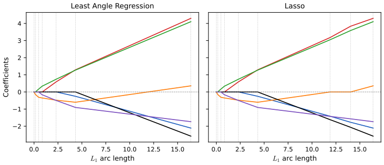
pp. 76–77 Why are the two paths so close? With standardised inputs, write the LAR tie as
\[ \bx_j^\T(\by-\bX\bb)=\gamma\cdot s_j,\quad\forall j\in\mathcal{A}, \tag{3.56} \]with \(|\bx_k^\T(\by-\bX\bb)|\le\gamma\) for \(k\notin\mathcal{A}\), and the lasso criterion in vector form,
\[ R(\bb)=\tfrac12\|\by-\bX\bb\|_2^2+\lambda\|\bb\|_1, \tag{3.57} \] \[ \bx_j^\T(\by-\bX\bb)=\lambda\cdot\sign(\beta_j),\quad\forall j\in\mathcal{B}, \tag{3.58} \] \[ |\bx_k^\T(\by-\bX\bb)|\le\lambda,\quad\forall k\notin\mathcal{B}. \tag{3.59} \](3.58)–(3.59) are Result 3.16 with \(\mathcal{B}\) the set of nonzero coefficients. They agree with (3.56) exactly when every active coefficient has the sign of its correlation.
Result 3.19 (LAR with modification 3.2a computes the lasso path) pp. 76–77; Exercise 3.27(c)
Assume each step has a unique event (one variable enters or leaves). Then Algorithm 3.2 with 3.2a produces a continuous, piecewise-linear path \(\bb(\gamma)\), \(\gamma\) decreasing from \(\lambda_{\max}\) to 0, and \(\bb(\gamma)\) is the lasso solution (3.52) at \(\lambda=\gamma\). Between consecutive knots the lasso path is linear in \(\lambda\):
\[ \hb(\lambda)=\hb(\lambda_0)-(\lambda-\lambda_0)\boldsymbol{\gamma}_0. \tag{3.90} \]If no coefficient ever reaches zero, the LAR and lasso paths coincide (as for the prostate data).
Filling the gap 3.10: why the modified LAR path satisfies the lasso conditions at every \(\lambda\) p. 77, "a heuristic argument"
Proof
We show by induction over the steps that at every point of the path, with \(\lambda\) the common value \(\gamma\) of the active \(|\bx_j^\T\br|\): (i) \(\bx_j^\T\br=\lambda s_j\) for \(j\) in the active set \(\mathcal{A}\), (ii) \(|\bx_k^\T\br|\le\lambda\) off \(\mathcal{A}\), (iii) \(\beta_j=0\) off \(\mathcal{A}\), and (iv) \(\sign\beta_j=s_j\) whenever \(\beta_j\ne0\). By Result 3.16, (i)–(iv) are exactly the lasso conditions at \(\lambda\).
Start. \(\bb=\mathbf{0}\), \(\lambda=\lambda_{\max}\), \(\mathcal{A}=\{\arg\max|\bx_j^\T\by|\}\): (i)–(iv) hold.
Within a step. By Result 3.18(a) the active inner products remain \(\lambda s_j\) as \(\lambda\) falls linearly; (ii) holds until an inactive input ties (the step is stopped there); (iii) holds as only active coefficients move. For (iv): each active coefficient moves linearly; a coefficient that has the sign \(s_j\) can lose it only by passing through zero, and the modification stops the step at that moment. A newly entered coefficient starts at zero and moves in direction \(\delta_j\); it must move with sign \(s_j\). Indeed, at the entry knot both "add \(j\)" and "keep \(j\) out" are candidate continuations; the KKT conditions (i)–(ii) just after the knot hold for the continuation in which the new coefficient has sign \(s_j\) (Efron et al., 2004, Lemma 5 show that, with one event at a time, the LAR direction of the enlarged set has \(\sign\delta_j=s_j\) for the entering variable; the same argument with roles reversed shows that a dropped variable's inner product then decreases strictly below \(\lambda\), so it stays out until it ties again).
At a drop. If \(\beta_j\) reaches 0, setting \(j\) inactive keeps (iii), and (ii) holds for \(j\) since \(|\bx_j^\T\br|=\lambda\) there; the new direction is recomputed on \(\mathcal{A}\setminus\{j\}\).
Linearity (3.90). On an interval with fixed active set \(\mathcal{A}\) and signs \(\bs\), (i) reads \(\bX_\mathcal{A}^\T(\by-\bX_\mathcal{A}\bb_\mathcal{A})=\lambda\bs\), so \(\bb_\mathcal{A}(\lambda)=(\bX_\mathcal{A}^\T\bX_\mathcal{A})^{-1}(\bX_\mathcal{A}^\T\by-\lambda\bs)\): affine in \(\lambda\), with \(\boldsymbol{\gamma}_0=(\bX_\mathcal{A}^\T\bX_\mathcal{A})^{-1}\bs\) (zero off \(\mathcal{A}\)). Since the lasso solution is unique (general position), the path is the lasso path. The code confirms this to \(10^{-9}\) against coordinate descent and scikit-learn at fixed \(\lambda\), and the knots against scikit-learn's lars_path, on three data sets including one with a drop. ∎
Degrees-of-freedom formula for LAR and lasso
pp. 77–79 For an adaptively fitted model, the number of parameters understates the complexity used (a best subset of size \(k\) has "used" more than \(k\)). The general definition is
\[ \df(\hat\by)=\frac{1}{\sigma^2}\sum_{i=1}^N\Cov(\hat y_i,y_i). \tag{3.60} \]Result 3.20 (degrees of freedom of linear fits, ridge and the lasso) pp. 77–79
Assume \(\by\sim\N(\boldsymbol{\mu},\sigma^2\bI)\). (a) For a linear fit \(\hat\by=\bS\by\) with \(\bS\) fixed, \(\df=\tr\bS\); least squares on \(k\) prespecified inputs has \(\df=k\) and ridge has \(\df=\tr\bS_\lambda\), (3.50). (b) (Stein) If \(\hat\by=g(\by)\) is almost differentiable with integrable partial derivatives, \(\df=\E\sum_i\partial\hat y_i/\partial y_i\). (c) For the lasso at fixed \(\lambda\), \(\df=\E|\mathcal{B}|\), the expected number of nonzero coefficients (Zou, Hastie and Tibshirani, 2007), so \(|\mathcal{B}|\) is an unbiased estimate.
Filling the gap 3.11: computing (3.60) p. 78, "it is easy to show", "something magical happens"
Derivation
(a) \[ \Cov(\hat y_i,y_i)=\Cov\big(\sum_kS_{ik}y_k,y_i\big)=S_{ii}\sigma^2 \] since the \(y\)'s are independent; summing gives \(\sigma^2\tr\bS\). For least squares \(\bS=\bH\), of trace \(k\) (Result 3.2).
(b) Stein's lemma. For \(Z\sim\N(\mu,\sigma^2)\) and absolutely continuous \(h\) with \(\E|h'(Z)|\lt \infty\), integration by parts against the density \(\phi\) (whose derivative is \(-\frac{z-\mu}{\sigma^2}\phi\)) gives \(\E[(Z-\mu)h(Z)]=\sigma^2\E h'(Z)\). Apply it to \(y_i\), conditionally on the other coordinates (independent of \(y_i\)): \[ \Cov(\hat y_i,y_i)=\E[(y_i-\mu_i)g_i(\by)]=\sigma^2\E\,\partial g_i/\partial y_i \].
(c) The lasso. Fix \(\lambda\). The fit \(\by\mapsto\bX\hb(\by)\) is continuous and piecewise linear in \(\by\) (it is the projection of \(\by\) onto a convex polytope translated, the dual of the lasso), hence Lipschitz and almost differentiable. Off a null set of \(\by\) the active set \(\mathcal{B}\) and signs \(\bs\) are locally constant, and by (3.58) \(\hb_\mathcal{B}=(\bX_\mathcal{B}^\T\bX_\mathcal{B})^{-1}(\bX_\mathcal{B}^\T\by-\lambda\bs)\), so locally \(\hat\by=\bH_\mathcal{B}\by-\)const with \(\bH_\mathcal{B}\) the projection on \(\col(\bX_\mathcal{B})\). Its divergence is \(\tr\bH_\mathcal{B}=|\mathcal{B}|\), and (b) gives \(\df=\E|\mathcal{B}|\). The null set where the active set changes does not matter because the fit is continuous there (this is the delicate part of Zou et al.'s proof).
Confirmed numerically on the prostate design (4000 simulated responses): the covariance definition gives 3.69 for the lasso at a fixed \(\lambda\) against \(\E|\mathcal{B}|=3.65\), and 6.31 for ridge against \(\tr\bS_\lambda=6.26\).
LAR after \(k\) steps. The book states that the degrees of freedom are then exactly \(k\). Efron et al. (2004) prove \(\df\approx k\) and exactness under a "positive cone" condition on \(\bX\) (which holds e.g. for orthogonal inputs); it is not exact in general. Our simulation on the prostate design gives 1.03, 1.99, 2.96 for \(k=1,2,3\): very close to \(k\). For best subset there is no such formula, and simulation shows \(\df>k\). ∎
For the lasso path (more than \(p\) steps when variables drop), \(\df\) is approximately the number of active predictors anywhere on the path, and works best at the last model with \(k\) predictors (Zou et al., 2007). In the shrinkage-paths demonstration the readout reports this number.
3.5 Methods Using Derived Input Directions
p. 79 When there are many correlated inputs, one can regress on a small number \(M\) of linear combinations \(Z_m\) of them. The methods differ in how the combinations are built.
3.5.1 Principal Components Regression
pp. 79–80 PCR uses the principal components \(\bz_m=\bX\bv_m\) of Section 3.4.1 (inputs standardised, as the components depend on scale). They are orthogonal, so the regression is a sum of univariate regressions:
\[ \hat\by^{\rm pcr}_{(M)}=\bar y\bone+\sum_{m=1}^M\hat\theta_m\bz_m,\qquad \hat\theta_m=\frac{\langle\bz_m,\by\rangle}{\langle\bz_m,\bz_m\rangle}, \tag{3.61} \] \[ \hb^{\rm pcr}(M)=\sum_{m=1}^M\hat\theta_m\bv_m. \tag{3.62} \]Result 3.21 (PCR in coefficient form; Exercise 3.13) p. 79
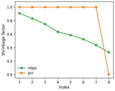
(3.62) holds, \(\hat\theta_m=\bu_m^\T\by/d_m\), and \(\hb^{\rm pcr}(p)=\hb^{\rm ls}\) when \(\bX\) has full rank. In the principal-component coordinates, PCR applies the factor 1 to components \(1,\dots,M\) and 0 to the rest, while ridge applies \(d_j^2/(d_j^2+\lambda)\) to all.
Proof
\(\bz_m=\bX\bv_m=d_m\bu_m\), so \(\langle\bz_m,\bz_m\rangle=d_m^2\) and \(\hat\theta_m=\bu_m^\T\by/d_m\). Then \(\sum_m\hat\theta_m\bz_m=\bX\sum_m\hat\theta_m\bv_m\): the coefficient vector is (3.62). With \(M=p\), \[ \sum_{m}\bv_m\bu_m^\T\by/d_m=\bV\bD^{-1}\bU^\T\by=(\bX^\T\bX)^{-1}\bX^\T\by \] (full rank, \(\bV\) square). In the basis \(\bv_j\), \(\bv_j^\T\hb^{\rm ls}=\bu_j^\T\by/d_j\), and \(\bv_j^\T\hb^{\rm pcr}\) equals this for \(j\le M\) and 0 otherwise; for ridge \(\bv_j^\T\hb^{\rm ridge}=\frac{d_j}{d_j^2+\lambda}\bu_j^\T\by\), the factor \(d_j^2/(d_j^2+\lambda)\) times the least-squares value. ∎
3.5.2 Partial Least Squares
pp. 80–82 PLS also builds directions, but uses \(\by\) to do it: the first direction weights each standardised input by its inner product with \(\by\).
Algorithm 3.3 (partial least squares) p. 81
- Standardise each \(\bx_j\) to mean 0 and variance 1. Set \(\hat\by^{(0)}=\bar y\bone\) and \(\bx_j^{(0)}=\bx_j\).
- For \(m=1,2,\dots,p\):
- \(\bz_m=\sum_{j=1}^p\hat\varphi_{mj}\bx_j^{(m-1)}\), where \(\hat\varphi_{mj}=\langle\bx_j^{(m-1)},\by\rangle\);
- \(\hat\theta_m=\langle\bz_m,\by\rangle/\langle\bz_m,\bz_m\rangle\);
- \(\hat\by^{(m)}=\hat\by^{(m-1)}+\hat\theta_m\bz_m\);
- orthogonalise each input with respect to \(\bz_m\): \[ \bx_j^{(m)}=\bx_j^{(m-1)}-\big[\langle\bz_m,\bx_j^{(m-1)}\rangle/\langle\bz_m,\bz_m\rangle\big]\bz_m \].
- Output the fitted vectors \(\{\hat\by^{(m)}\}_1^p\); they are linear in the \(\bx_j\), \(\hat\by^{(m)}=\bX\hb^{\rm pls}(m)\), and the coefficients are recovered from the sequence of transformations: if \(\bX^{(m-1)}=\bX\mathbf{T}_{m-1}\), then \(\bz_m=\bX(\mathbf{T}_{m-1}\hat{\boldsymbol\varphi}_m)\) (this is how the code and the demonstration do it; they agree with scikit-learn's PLS to \(10^{-9}\)).
PLS seeks directions of high variance and high correlation with the response. The \(m\)th principal component direction solves
\[ \max_{\ba}\Var(\bX\ba)\quad\text{subject to }\|\ba\|=1,\ \ba^\T\bS\bv_\ell=0,\ \ell=1,\dots,m-1, \tag{3.63} \](\(\bS\) the sample covariance of the inputs; the side conditions make \(\bz_m\) uncorrelated with the earlier components), and the \(m\)th PLS direction solves
\[ \max_{\ba}\Corr^2(\by,\bX\ba)\Var(\bX\ba)\quad\text{subject to }\|\ba\|=1,\ \ba^\T\bS\hat{\boldsymbol\varphi}_\ell=0,\ \ell=1,\dots,m-1. \tag{3.64} \]Result 3.22 (properties of PLS; Exercises 3.14, 3.15) pp. 81–82
(a) The \(\bz_m\) are mutually orthogonal, so \(\hat\by^{(m)}\) is the projection of \(\by\) onto \(\mathrm{span}(\bz_1,\dots,\bz_m)\), and \(\hat\by^{(p)}\) is the least-squares fit when \(\bX\) has full rank. (b) The first PLS direction \(\hat{\boldsymbol\varphi}_1=\bX^\T\by\) (normalised) solves (3.64) with \(m=1\); later ones solve it with the side conditions. (c) If the standardised inputs are orthogonal, PLS reaches least squares at \(m=1\) and \(\hat{\boldsymbol\varphi}_m=\mathbf{0}\) for \(m>1\).
Proof
(a) Step (d) makes every \(\bx_j^{(m)}\) orthogonal to \(\bz_m\), and inductively to \(\bz_1,\dots,\bz_m\) (removing a multiple of \(\bz_m\), itself orthogonal to the earlier \(\bz\)'s, preserves orthogonality to them). \(\bz_{m+1}\) is a combination of the \(\bx_j^{(m)}\), hence orthogonal to \(\bz_1,\dots,\bz_m\). Then (b)–(c) of step 2 add successive univariate regressions on orthogonal vectors (Result 3.7), which is the projection. The \(\bz\)'s lie in \(\col(\bX)\); if \(p\) of them are nonzero they span it, and the projection is least squares. (If some \(\hat{\boldsymbol\varphi}_m=\mathbf{0}\), then \(\by-\hat\by^{(m-1)}\perp\col(\bX)\) already, as shown in (c).)
(b) For centred \(\by\) and \(\bX\), \[ \Corr^2(\by,\bX\ba)\Var(\bX\ba)=\frac{(\by^\T\bX\ba)^2}{\|\by\|^2\|\bX\ba\|^2}\cdot\frac{\|\bX\ba\|^2}{N}=\frac{(\ba^\T\bX^\T\by)^2}{N\|\by\|^2} \]. Over unit \(\ba\), by Cauchy–Schwarz the maximum is at \(\ba\propto\bX^\T\by=\hat{\boldsymbol\varphi}_1\): the variance factors cancel and only the covariance with \(\by\) remains, so "high variance and high correlation" means "high covariance". For \(m>1\), \(\hat{\boldsymbol\varphi}_m\propto\bX^{(m-1)\T}\by\), the same Cauchy–Schwarz argument applied to the deflated inputs, whose span is orthogonal to the earlier \(\bz_\ell=\bX\boldsymbol\varphi_\ell\); this orthogonality is the condition \(\ba^\T\bS\hat{\boldsymbol\varphi}_\ell=0\) once the direction is expressed in terms of the original inputs (Stone and Brooks, 1990, Frank and Friedman, 1993).
(c) If \(\bX^\T\bX=c\bI\) then \(\bz_1=\bX\bX^\T\by\) and \(\hat\by^{(1)}=\bz_1\langle\bz_1,\by\rangle/\|\bz_1\|^2\) with \(\|\bz_1\|^2=c\|\bX^\T\by\|^2\) and \(\langle\bz_1,\by\rangle=\|\bX^\T\by\|^2\): \(\hat\by^{(1)}=\bX\bX^\T\by/c=\bH\by\), least squares. The residual is orthogonal to every \(\bx_j\), and \(\bx_j^{(1)}=\bx_j-\bz_1\langle\bz_1,\bx_j\rangle/\|\bz_1\|^2\) gives \[ \hat\varphi_{2j}=\langle\bx_j,\by\rangle-\langle\bz_1,\bx_j\rangle\langle\bz_1,\by\rangle/\|\bz_1\|^2=\langle\bx_j,\by-\hat\by^{(1)}\rangle=0 \]. ∎
Result 3.23 (PLS is conjugate gradients, with polynomial shrinkage factors; Exercise 3.18) pp. 82–83
Let \(\bG=\bX^\T\bX\) and \[ \mathcal{K}_m=\mathrm{span}\{\bX^\T\by,\bG\bX^\T\by,\dots,\bG^{m-1}\bX^\T\by\} \]. (a) \(\hb^{\rm pls}(m)\) minimises \(\|\by-\bX\bb\|^2\) over \(\bb\in\mathcal{K}_m\); it equals the \(m\)th iterate of the conjugate gradient method for \(\bG\bb=\bX^\T\by\) started at \(\mathbf{0}\). (b) In principal-component coordinates, \(\bv_j^\T\hb^{\rm pls}(m)=f_j\,\bv_j^\T\hb^{\rm ls}\) with
\[ f_j=1-\prod_{k=1}^m\Big(1-\frac{d_j^2}{\theta_k}\Big), \]where \(\theta_1,\dots,\theta_m\) are distinct and lie strictly between \(d_p^2\) and \(d_1^2\). Components with \(d_j^2\) below all \(\theta_k\) are shrunk (\(0\le f_j\lt 1\)), more so the smaller \(d_j\); but \(f_j>1\) whenever an odd number of \(\theta_k\) lie below \(d_j^2\) and the product is negative. This is the book's remark that PLS "can actually inflate some of the higher variance directions".
Filling the gap 3.12: PLS, Krylov subspaces and inflation pp. 82–83, "it can be shown"
Derivation
(a) Krylov. Let \(\bP_{m}\) project onto \(\mathrm{span}(\bz_1,\dots,\bz_{m})\). Step (d) gives \(\bX^{(m)}=(\bI-\bP_m)\bX\), so \[ \hat{\boldsymbol\varphi}_{m+1}=\bX^\T(\bI-\bP_m)\by=\bX^\T(\by-\hat\by^{(m)})=\bX^\T\by-\bG\hb^{\rm pls}(m) \]. By induction suppose \(\mathrm{span}(\bz_1..\bz_m)=\bX\mathcal{K}_m\) and \(\hb^{\rm pls}(m)\in\mathcal{K}_m\). Then \(\hat{\boldsymbol\varphi}_{m+1}\in\mathcal{K}_{m+1}\) and \(\bz_{m+1}=(\bI-\bP_m)\bX\hat{\boldsymbol\varphi}_{m+1}\in\bX\mathcal{K}_{m+1}\), so \(\mathrm{span}(\bz_1..\bz_{m+1})\subseteq\bX\mathcal{K}_{m+1}\), with equality by dimension when the \(\bz\)'s are nonzero. Hence \(\hat\by^{(m)}\) is the projection of \(\by\) onto \(\bX\mathcal{K}_m\), i.e. \(\hb^{\rm pls}(m)\) minimises \(\|\by-\bX\bb\|^2\) over \(\mathcal{K}_m\). Conjugate gradients on \(\bG\bb=\bX^\T\by\) from \(\mathbf{0}\) produces the minimiser of \[ (\bb-\hb^{\rm ls})^\T\bG(\bb-\hb^{\rm ls})=\|\bX\bb-\bX\hb^{\rm ls}\|^2 \] over the same \(\mathcal{K}_m\) (its defining property), and \[ \|\by-\bX\bb\|^2=\|\by-\bX\hb^{\rm ls}\|^2+\|\bX\bb-\bX\hb^{\rm ls}\|^2 \]: the same minimiser. (Confirmed numerically: the iterates agree to \(10^{-8}\) for \(m=1,\dots,8\).)
(b) The polynomial. Every \(\bb\in\mathcal{K}_m\) is \(\pi(\bG)\bX^\T\by\) for a polynomial \(\pi\) of degree \(\lt m\). With \(t_j=d_j^2\) and \(w_j=(\bu_j^\T\by)^2\): \(\bv_j^\T\bb=\pi(t_j)d_j\bu_j^\T\by=t_j\pi(t_j)\cdot\bv_j^\T\hb^{\rm ls}\), so \(f_j=t_j\pi(t_j)=1-q(t_j)\) with \(q(t)=1-t\pi(t)\), a polynomial of degree \(\le m\) with \(q(0)=1\). The residual is \[ \|\by-\bX\bb\|^2=\|\by-\bH\by\|^2+\sum_jw_jq(t_j)^2 \], so PLS chooses the \(q\) that minimises \(\sum_jw_jq(t_j)^2\) subject to \(q(0)=1\). Perturbing \(q\) by \(\varepsilon\,t\,r(t)\) (which keeps \(q(0)=1\)) for any \(r\) of degree \(\lt m\) gives the optimality condition \(\sum_jw_jt_jq(t_j)r(t_j)=0\): \(q\) is orthogonal to all polynomials of degree \(\lt m\) for the discrete measure with positive masses \(w_jt_j\) at the points \(t_j\).
The roots. Suppose \(q\) changed sign at only \(k\lt m\) points \(\theta_1,\dots,\theta_k\) of \((t_p,t_1)\). Take \(r(t)=\prod_{i\le k}(t-\theta_i)\), of degree \(k\lt m\): then \(q\,r\) has one sign at all the \(t_j\) and is not zero at all of them (\(q\ne0\) as \(q(0)=1\), and with at least \(m+1\) support points \(q\) cannot vanish on all), so \(\sum_jw_jt_jq(t_j)r(t_j)\ne0\), a contradiction. Hence \(q\) has \(m\) distinct sign changes in \((t_p,t_1)\), i.e. \(m\) distinct roots \(\theta_k\) there, and with \(q(0)=1\), \(q(t)=\prod_k(1-t/\theta_k)\). (The \(\theta_k\) are the Ritz values of the Lanczos method.)
Shrinking and inflating. For \(t\lt \min_k\theta_k\) every factor lies in \((0,1]\), so \(0\lt q\le1\) and \(0\le f\lt 1\), decreasing in \(t\) towards 0: low-variance components are shrunk. Beyond the smallest root \(q\) alternates in sign; where it is negative, \(f_j=1-q(t_j)>1\). On the prostate data with \(m=1\) the single root is the Rayleigh quotient \(\theta_1=\hat{\boldsymbol\varphi}_1^\T\bG\hat{\boldsymbol\varphi}_1/\|\hat{\boldsymbol\varphi}_1\|^2\), and \(f_1=1.074\); with \(m=2\), \(f_2=1.315\) (pcr-pls demonstration, preset 2). ∎
So PLS shrinks the low-variance directions like ridge and PCR, but can inflate others, which makes it a little less stable; Frank and Friedman (1993) found ridge generally preferable for prediction, with PCR and PLS only slightly behind. In the prostate example cross-validation chose \(M=2\) PLS directions (the last column of Table 3.3).
3.6 Discussion: A Comparison of the Selection and Shrinkage Methods
pp. 82–84 Two correlated inputs with correlation \(\rho\) and true coefficients \(\bb=(4,2)\) show how the methods move from 0 to the least-squares solution.
Result 3.24 (the paths of Figure 3.18 in closed form) p. 84
Take the population version \(\bX^\T\bX=\bG=\begin{pmatrix}1&\rho\\\rho&1\end{pmatrix}\), \(\bX^\T\by=\bG\bb=\bc\), so least squares is exactly \(\bb=(4,2)\), \(\bc=(4+2\rho,\,4\rho+2)\). Then: ridge is the curve \((\bG+\lambda\bI)^{-1}\bc\); best subset of size 1 is \((c_1,0)\) if \(|c_1|\ge|c_2|\); PCR with one component is \(\bv\bv^\T\bb\) with \(\bv=(1,\pm1)/\sqrt2\) the leading eigenvector (sign of \(\rho\)); PLS with one direction is \(\theta\bc\), \(\theta=\|\bc\|^2/\bc^\T\bG\bc\); the lasso moves along the \(\beta_1\) axis to \((2,0)\) (for \(\rho=\pm0.5\)) and then straight to \((4,2)\). For \(\rho=0.5\): best subset \((5,0)\), PCR \((3,3)\), PLS \((3.361,2.689)\). For \(\rho=-0.5\): best subset \((3,0)\), PCR \((1,-1)\), PLS \((3,0)\).
Proof
Ridge is (3.44). Best subset of size one keeps the input with the larger \(|c_j|\) (largest RSS reduction \(c_j^2/G_{jj}\), Result 3.11 from the empty model) with coefficient \(c_j\). PCR: \(\bG\) has eigenvalues \(1\pm\rho\) with eigenvectors \((1,\pm1)/\sqrt2\); one component gives \(\bv(\bv^\T\bc)/(1+|\rho|)=\bv\bv^\T\bb\). For \(\rho=0.5\), \(\bv\bv^\T(4,2)=(3,3)\); for \(\rho=-0.5\), \(\bv=(1,-1)/\sqrt2\) and \((1,-1)\). PLS: \(\hat{\boldsymbol\varphi}_1=\bc\) and \(\hat\theta_1\) is the least-squares coefficient on \(\bz=\bX\bc\), \(\bc^\T\bc/\bc^\T\bG\bc\): for \(\rho=0.5\), \(\bc=(5,4)\), \(\theta=41/61\), giving \((3.361,2.689)\); for \(\rho=-0.5\), \(\bc=(3,0)\), \(\theta=1\), giving \((3,0)\). Lasso: by Result 3.19, \(\beta_1=c_1-\lambda\) while \(|c_2-\rho\beta_1|\lt \lambda\); for \(\rho=0.5\), \(c_2-\rho(5-\lambda)=1.5+0.5\lambda=\lambda\) at \(\lambda=3\), \(\beta_1=2\); for \(\rho=-0.5\), \(|0+0.5(3-\lambda)|=\lambda\) at \(\lambda=1\), \(\beta_1=2\). After that both coordinates move linearly to \((4,2)\). PLS and PCR with two directions are least squares. ∎
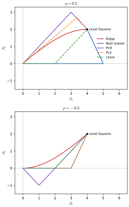
In summary, PLS, PCR and ridge behave similarly; ridge may be preferred because it shrinks smoothly rather than in discrete steps. The lasso falls between ridge and best subset and has some properties of each.
3.7 Multiple Outcome Shrinkage and Selection
pp. 84–86 The separate least-squares fits of Section 3.2.4 can be shrunk one output at a time (with \(K\) penalties) or with a common penalty. Correlated responses suggest pooling: if
\[ Y_k=f(X)+\varepsilon_k \tag{3.65} \] \[ Y_\ell=f(X)+\varepsilon_\ell, \tag{3.66} \]the observations on \(Y_k\) and \(Y_\ell\) should be pooled to estimate the common \(f\). Canonical correlation analysis finds uncorrelated combinations \(\bX\bv_m\) of the inputs and \(\bY\bu_m\) of the (centred) responses that successively maximise
\[ \Corr^2(\bY\bu_m,\bX\bv_m), \tag{3.67} \]for at most \(M=\min(K,p)\) pairs. Reduced-rank regression (Izenman, 1975; van der Merwe and Zidek, 1980) solves
\[ \hat\bB^{\rm rr}(m)=\argmin_{\rank(\bB)=m}\sum_{i=1}^N(y_i-\bB^\T x_i)^\T\mathbf{\Sigma}^{-1}(y_i-\bB^\T x_i). \tag{3.68} \]With \(\mathbf{\Sigma}\) estimated by \(\bY^\T\bY/N\),
\[ \hat\bB^{\rm rr}(m)=\hat\bB\bU_m\bU_m^-, \tag{3.69} \] \[ \hat\bB^{\rm rr}(m)=(\bX^\T\bX)^{-1}\bX^\T(\bY\bU_m)\bU_m^-, \tag{3.70} \] \[ \hat\bY^{\rm rr}(m)=\bX(\bX^\T\bX)^{-1}\bX^\T\bY\bU_m\bU_m^-=\bH\bY\bP_m, \tag{3.71} \]where \(\bU_m\) holds the first \(m\) left canonical vectors and \(\bU_m^-\) is a generalised inverse; \(\bP_m\) is the rank-\(m\) CCA response projection. Reduced-rank regression regresses on the pooled responses \(\bY\bU_m\) and maps back.
Result 3.25 (CCA and reduced-rank regression; Exercises 3.20–3.22) pp. 85–86, (3.86)–(3.87)
(a) With \(\bY^\T\bY\), \(\bX^\T\bX\) invertible, the leading canonical pair solves \(\max\bu^\T(\bY^\T\bX)\bv\) subject to \(\bu^\T\bY^\T\bY\bu=1\), \(\bv^\T\bX^\T\bX\bv=1\), and is \(\bu_1=(\bY^\T\bY)^{-1/2}\bu_1^*\), \(\bv_1=(\bX^\T\bX)^{-1/2}\bv_1^*\), with \(\bu_1^*,\bv_1^*\) the leading singular vectors of \[ (\bY^\T\bY)^{-1/2}\bY^\T\bX(\bX^\T\bX)^{-1/2}=\bU^*\bD^*\bV^{*\T} \]; the later pairs are the later singular vectors. (b) The solution of (3.68) with \(\mathbf{\Sigma}=\bY^\T\bY/N\) is (3.69) with \(\bU_m=\mathbf{\Sigma}^{-1/2}\bU^*_m\) and \(\bU_m^-=\bU_m^{*\T}\mathbf{\Sigma}^{1/2}\). (c) The same \(\hat\bB^{\rm rr}(m)\) results if \(\mathbf{\Sigma}\) is the residual covariance \((\bY-\bX\hat\bB)^\T(\bY-\bX\hat\bB)/(N-pK)\).
Filling the gap 3.13: reduced rank regression is a truncated SVD after whitening p. 85, "one can show"
Derivation
(a) Substitute \(\bu=(\bY^\T\bY)^{-1/2}\ba\), \(\bv=(\bX^\T\bX)^{-1/2}\mathbf{b}\): the constraints become \(\|\ba\|=\|\mathbf{b}\|=1\) and the objective \(\ba^\T\mathbf{K}\mathbf{b}\) with \(\mathbf{K}=(\bY^\T\bY)^{-1/2}\bY^\T\bX(\bX^\T\bX)^{-1/2}\). Its maximum over unit vectors is the largest singular value, at the leading singular pair (variational characterisation of the SVD). The correlation of \(\bY\bu\) and \(\bX\bv\) is exactly \(\bu^\T\bY^\T\bX\bv\) under the constraints, so this maximises (3.67). The \(m\)th pair maximises the same form subject to orthogonality to the previous \(\ba,\mathbf{b}\), i.e. to uncorrelatedness of the variates, and is the \(m\)th singular pair.
(b) Let \(\mathbf{W}=\mathbf{\Sigma}^{-1/2}\) and \(\bY^*=\bY\mathbf{W}\), \(\bB^*=\bB\mathbf{W}\) (same rank). The criterion is \[ \|\bY^*-\bX\bB^*\|_F^2=\|\bY^*-\bH\bY^*\|_F^2+\|\bH\bY^*-\bX\bB^*\|_F^2 \] (Pythagoras: \(\bX\bB^*\in\col(\bX)\)). The second term is minimised over rank \(m\) by the truncated SVD of \(\bH\bY^*\) (Eckart–Young), \(\bH\bY^*\mathbf{Q}_m\mathbf{Q}_m^\T\) with \(\mathbf{Q}_m\) its top \(m\) right singular vectors, which is attainable as \(\bX\hat\bB\mathbf{W}\mathbf{Q}_m\mathbf{Q}_m^\T\). So \(\hat\bB^{\rm rr}=\hat\bB\mathbf{W}\mathbf{Q}_m\mathbf{Q}_m^\T\mathbf{W}^{-1}\). The right singular vectors of \(\bH\bY^*\) are eigenvectors of \[ \mathbf{W}\bY^\T\bH\bY\mathbf{W}=\mathbf{W}\bY^\T\bX(\bX^\T\bX)^{-1}\bX^\T\bY\mathbf{W} \]. With \(\mathbf{W}=\sqrt N(\bY^\T\bY)^{-1/2}\) this is \(N\mathbf{K}\mathbf{K}^\T\), whose eigenvectors are the left singular vectors \(\bU^*\) of \(\mathbf{K}\). Hence \(\mathbf{Q}_m=\bU^*_m\) and \(\hat\bB^{\rm rr}=\hat\bB(\mathbf{\Sigma}^{-1/2}\bU^*_m)(\bU_m^{*\T}\mathbf{\Sigma}^{1/2})\), which is (b); \(\bU_m^-\bU_m=\bI_m\) shows it is a generalised inverse.
(c) With \(\mathbf{E}=\bY-\bH\bY\), \(\bY^\T\bY=\bY^\T\bH\bY+\mathbf{E}^\T\mathbf{E}\). The relevant eigenproblem with \(\mathbf{\Sigma}_E\propto\mathbf{E}^\T\mathbf{E}\) is \(\bY^\T\bH\bY\mathbf{a}=\mu\,\mathbf{E}^\T\mathbf{E}\mathbf{a}\) (generalised); with \(\mathbf{\Sigma}\propto\bY^\T\bY\) it is \(\bY^\T\bH\bY\mathbf{a}=\nu(\bY^\T\bH\bY+\mathbf{E}^\T\mathbf{E})\mathbf{a}\), i.e. the same \(\mathbf{a}\) with \(\mu=\nu/(1-\nu)\), a monotone map that preserves the order. The rank-\(m\) solution depends on \(\mathbf{\Sigma}\) only through the span of the leading generalised eigenvectors (and the scaling constant cancels in \(\bU_m\bU_m^-\)), so it is unchanged. Confirmed numerically for both choices against a direct minimisation. ∎
pp. 86–87 Breiman and Friedman (1997) shrink the canonical variates smoothly instead of truncating them ("curds and whey"):
\[ \hat\bB^{c+w}=\hat\bB\bU\mathbf{\Lambda}\bU^{-1}, \tag{3.72} \] \[ \lambda_m=\frac{c_m^2}{c_m^2+\frac pN(1-c_m^2)},\quad m=1,\dots,M, \tag{3.73} \] \[ \hat\bY^{c+w}=\bH\bY\bS^{c+w}, \tag{3.74} \]with \(c_m\) the canonical correlations and \(\bS^{c+w}=\bU\mathbf{\Lambda}\bU^{-1}\) the response shrinkage operator; the factors tend to 1 as \(p/N\to0\). Shrinking in both spaces gives
\[ \hat\bY^{\rm ridge,c+w}=\mathbf{A}_\lambda\bY\bS^{c+w}, \tag{3.75} \]with \(\mathbf{A}_\lambda=\bX(\bX^\T\bX+\lambda\bI)^{-1}\bX^\T\) the ridge operator.
3.8 More on the Lasso and Related Path Algorithms
p. 86 Since LAR, many path algorithms have been developed, and \(L_1\) regularisation has grown into a field of its own (compressed sensing; Donoho, 2006; Candès, 2006).
3.8.1 Incremental Forward Stagewise Regression
Algorithm 3.4 (incremental forward stagewise regression, FSε) p. 86
- Start with \(\br=\by\) and \(\beta_1=\dots=\beta_p=0\), predictors standardised to mean zero and unit norm.
- Find the predictor \(\bx_j\) most correlated with \(\br\).
- Update \(\beta_j\leftarrow\beta_j+\delta_j\), \(\delta_j=\epsilon\cdot\sign\langle\bx_j,\br\rangle\), with a small \(\epsilon>0\), and set \(\br\leftarrow\br-\delta_j\bx_j\).
- Repeat steps 2–3 many times, until the residuals are uncorrelated with all the predictors.
With \(\delta_j=\langle\bx_j,\br\rangle\) instead (a full step) this is the forward stagewise regression of Section 3.3.3. As \(\epsilon\to0\) the profiles converge to a limit, infinitesimal forward stagewise FS0, which the book calls "L2boost" after Bühlmann and Hothorn (2007); it is the linear version of boosting (Chapters 10 and 16).
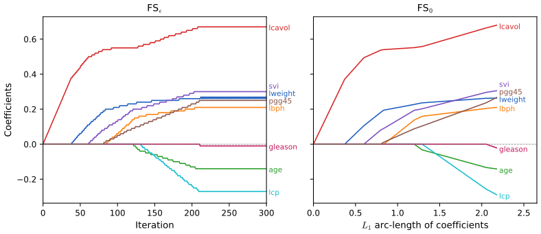
Algorithm 3.2b (least angle regression: FS0 modification) p. 88
- Find the new direction by solving the constrained least-squares problem \(\min_{\mathbf{b}}\|\br-\bX_\mathcal{A}\mathbf{b}\|_2^2\) subject to \(b_js_j\ge0\), \(j\in\mathcal{A}\), where \(s_j\) is the sign of \(\langle\bx_j,\br\rangle\).
Result 3.26 (what the FS0 direction does) p. 88
Let the solution \(\mathbf{b}\) of 3.2b have support \(\mathcal{M}\subseteq\mathcal{A}\) (the variables that move). Along \(\bu=\bX_\mathcal{A}\mathbf{b}\), the inner products of the moving variables stay tied and fall at the common rate, while those of the tied-but-not-moving variables fall at least as fast, so those variables leave the tie. Every coefficient moves in the direction of its current correlation, which is the defining property of FSε. Consequently, if the LAR profiles are monotone, LAR, lasso and FS0 coincide; if they are not monotone but never cross zero, LAR and lasso coincide.
Filling the gap 3.14: the non-negative least-squares direction p. 88, "one can show"
Derivation
Write \(\mathbf{b}=\bs\circ\mathbf{c}\) with \(\mathbf{c}\ge\mathbf{0}\) and \(\tilde\bX=\bX_\mathcal{A}\diag(\bs)\). The KKT conditions of \(\min_{\mathbf{c}\ge0}\|\br-\tilde\bX\mathbf{c}\|^2\) are \(\tilde\bx_j^\T(\br-\tilde\bX\mathbf{c})=0\) if \(c_j>0\) and \(\le0\) if \(c_j=0\). In terms of \(\bu=\tilde\bX\mathbf{c}\): \(s_j\bx_j^\T\bu=s_j\bx_j^\T\br=C\) for moving \(j\), and \(s_j\bx_j^\T\bu\ge C\) for non-moving tied \(j\). Along \(\br-\alpha\bu\), \(s_j\bx_j^\T(\br-\alpha\bu)=C(1-\alpha)\) for moving and \(\le C(1-\alpha)\) for non-moving variables: the latter drop below the maximum, as claimed, and the code removes them from the tied set (they may tie again later). Each moving coefficient changes by \(\alpha b_j\) with \(\sign b_j=s_j\), the sign of its correlation, exactly as each FSε step moves \(\beta_j\) by \(\epsilon\,\sign\langle\bx_j,\br\rangle\); in the limit, the tied variables share the increments in the proportions that keep them tied (Hastie et al., 2007). If the plain LAR direction already has \(\sign\delta_j=s_j\) for all active \(j\) (monotone profiles), it solves 3.2b, so FS0 = LAR; if moreover no coefficient reaches zero, the lasso equals both (Result 3.19).
Confirmed numerically. On the simulated data of Figure 3.15, FSε stays within 0.011 of the exact FS0 path for \(\epsilon=0.01\) and within 0.001 for \(\epsilon=0.001\) (error proportional to \(\epsilon\)), while it departs from the lasso path by 0.46: there FS0 differs from the lasso (x2 is frozen at \(-0.60\) for a stretch instead of being shrunk to zero and dropped). ∎
FS0 optimises progress in residual sum of squares per unit of \(L_1\) arc length (the lasso does so per unit increase of \(\|\bb\|_1\)), which discourages changes of direction: a monotone version of the lasso, with smoother profiles that may help when \(p\gg N\).
3.8.2 Piecewise-Linear Path Algorithms
p. 89 Consider
\[ \hb(\lambda)=\argmin_{\bb}\,[R(\bb)+\lambda J(\bb)], \tag{3.76} \] \[ R(\bb)=\sum_{i=1}^NL\Big(y_i,\beta_0+\sum_{j=1}^px_{ij}\beta_j\Big), \tag{3.77} \]with \(L\) and \(J\) convex. Rosset and Zhu (2007) show the path is piecewise linear if \(R\) is quadratic or piecewise quadratic and \(J\) is piecewise linear (squared or absolute loss, Huberised losses; \(L_1\) and \(L_\infty\) penalties; and, in the dual, the hinge loss of the support vector machine, Section 12.3.5).
Result 3.27 (why such paths are piecewise linear) p. 89
If on a region of \(\bb\)-space \(R(\bb)=\frac12\bb^\T\mathbf{A}\bb-\mathbf{g}^\T\bb\) with \(\mathbf{A}\succ0\) on the relevant coordinates, and \(J\) is linear on a cone (fixed signs, fixed active set), then while the solution stays in that piece, \(\hb(\lambda)=\mathbf{A}^{-1}(\mathbf{g}-\lambda\nabla J)\), linear in \(\lambda\); the path is a union of such segments, with knots where the piece changes.
Proof
On the piece, the optimality condition is \(\mathbf{A}\bb-\mathbf{g}+\lambda\mathbf{s}=\mathbf{0}\) with \(\mathbf{s}=\nabla J\) constant (restricted to the free coordinates, the others being fixed at the piece's boundary values, e.g. 0), whose solution is affine in \(\lambda\). The solution path is continuous in \(\lambda\) (strict convexity on the free coordinates), so consecutive segments join at knots. (3.90) is the lasso instance. ∎
3.8.3 The Dantzig Selector
pp. 89–90 Candès and Tao (2007) proposed
\[ \min_{\bb}\|\bb\|_1\ \text{ subject to }\ \|\bX^\T(\by-\bX\bb)\|_\infty\le s, \tag{3.78} \]equivalently
\[ \min_{\bb}\|\bX^\T(\by-\bX\bb)\|_\infty\ \text{ subject to }\ \|\bb\|_1\le t. \tag{3.79} \]Result 3.28 (the Dantzig selector is a linear programme) p. 89
With \(\bb=\bb^+-\bb^-\), \(\bb^\pm\ge\mathbf{0}\), \(\bG=\bX^\T\bX\), \(\bc=\bX^\T\by\), (3.78) is the LP: minimise \(\bone^\T(\bb^++\bb^-)\) subject to \(\bG(\bb^+-\bb^-)\le s\bone+\bc\) and \(-\bG(\bb^+-\bb^-)\le s\bone-\bc\). As \(s\to0\) the solution tends to the least-squares solution when \(N>p\) (full rank), and to the minimum-\(L_1\)-norm least-squares solution when \(p\ge N\).
Proof
\(\|\bc-\bG\bb\|_\infty\le s\) is the pair of linear inequalities stated; at an optimum \(\min(\beta_j^+,\beta_j^-)=0\) (otherwise subtract the minimum from both, keeping feasibility and lowering the objective), so the objective equals \(\|\bb\|_1\). At \(s=0\) the constraint is the normal equations \(\bG\bb=\bc\); with full column rank their only solution is \(\hb^{\rm ls}\), and when \(p\ge N\) the solutions form an affine set of least-squares solutions, of which the LP picks the one of minimum \(L_1\) norm. (The code's LP solution at \(s=10^{-9}\) equals least squares on the prostate data to \(10^{-6}\).) ∎
The lasso keeps the active inner products tied at the maximum and decreasing (Exercise 3.23), always larger than the inactive ones. The Dantzig selector minimises the maximum inner product instead; it can achieve a smaller maximum, but the variables tied at the maximum need not be the active ones, so it can include a variable less correlated with the residual than some excluded one (Efron et al., 2007), and its paths can be erratic. The same recovery properties hold for the lasso (Bickel et al., 2009).
3.8.4 The Grouped Lasso
pp. 90–91 When the predictors come in groups (dummies of one factor, genes of one pathway), the grouped lasso (Bakin, 1999; Lin and Zhang, 2006; Yuan and Lin, 2006) penalises the unsquared Euclidean norm of each group's coefficients:
\[ \min_{\bb\in\R^p}\Big(\Big\|\by-\beta_0\bone-\sum_{\ell=1}^L\bX_\ell\bb_\ell\Big\|_2^2+\lambda\sum_{\ell=1}^L\sqrt{p_\ell}\,\|\bb_\ell\|_2\Big). \tag{3.80} \]Result 3.29 (whole groups drop out) p. 90
\(\hb\) solves (3.80) (centred data) iff for every group, with \(\br_\ell=\by-\sum_{k\ne\ell}\bX_k\hb_k\): \(\hb_\ell=\mathbf{0}\) when \(\|\bX_\ell^\T\br_\ell\|_2\le\lambda\sqrt{p_\ell}/2\), and otherwise \(2\bX_\ell^\T(\br_\ell-\bX_\ell\hb_\ell)=\lambda\sqrt{p_\ell}\,\hb_\ell/\|\hb_\ell\|\). If \(\bX_\ell^\T\bX_\ell=\bI\), the block solution is the group soft-threshold \(\hb_\ell=\big(1-\frac{\lambda\sqrt{p_\ell}}{2\|\mathbf{s}_\ell\|}\big)_+\mathbf{s}_\ell\) with \(\mathbf{s}_\ell=\bX_\ell^\T\br_\ell\).
Proof
The subdifferential of \(\|\bb_\ell\|_2\) is \(\{\bb_\ell/\|\bb_\ell\|\}\) if \(\bb_\ell\ne\mathbf{0}\) and the unit ball otherwise (the norm is not differentiable only at 0, where every vector of norm \(\le1\) is a subgradient, by Cauchy–Schwarz). Setting \(\mathbf{0}\in\partial\) of (3.80) block by block gives the conditions. With orthonormal \(\bX_\ell\), the block problem is \(\|\mathbf{s}_\ell-\bb_\ell\|^2+\lambda\sqrt{p_\ell}\|\bb_\ell\|\)+const; the solution is parallel to \(\mathbf{s}_\ell\), and the one-dimensional problem in its length \(r\ge0\), \((\|\mathbf{s}_\ell\|-r)^2+\lambda\sqrt{p_\ell}r\), is minimised at \(r=(\|\mathbf{s}_\ell\|-\lambda\sqrt{p_\ell}/2)_+\). Because the norm is zero only when the whole block is zero, entire groups are set to zero; within a selected group, coefficients are generally all nonzero. (The code's block coordinate descent satisfies these conditions to \(10^{-8}\) and zeroes a whole group in its test case.) ∎
Generalisations use norms \(\|\boldsymbol\eta\|_\mathbf{K}=(\boldsymbol\eta^\T\mathbf{K}\boldsymbol\eta)^{1/2}\), overlapping groups (Zhao et al., 2009), and sparse additive models (Ravikumar et al., 2009).
3.8.5 Further Properties of the Lasso
pp. 91–92 Many authors study when the lasso recovers the correct model as \(N\) and \(p\) grow (Knight and Fu, 2000; Greenshtein and Ritov, 2004; Meinshausen and Bühlmann, 2006; Zhao and Yu, 2006; Wainwright, 2009; and others). A typical condition on the design is
\[ \|(\bX_\mathcal{S}^\T\bX_\mathcal{S})^{-1}\bX_\mathcal{S}^\T\bX_{\mathcal{S}^c}\|_\infty\le(1-\epsilon)\ \text{ for some }\epsilon\in(0,1], \tag{3.81} \]with \(\mathcal{S}\) the true support: the regression coefficients of the noise variables on the true ones are not too large (the "irrepresentable" condition). The matrix norm here is the maximum absolute column sum of \((\bX_\mathcal{S}^\T\bX_\mathcal{S})^{-1}\bX_\mathcal{S}^\T\bX_{\mathcal{S}^c}\), i.e. \(\max_{k\in\mathcal{S}^c}\|(\bX_\mathcal{S}^\T\bX_\mathcal{S})^{-1}\bX_\mathcal{S}^\T\bx_k\|_1\).
Filling the gap 3.15: why (3.81) is needed for the lasso to find the right variables p. 91
Derivation (noiseless case)
Let \(\by=\bX_\mathcal{S}\bb_\mathcal{S}\) exactly, with sign vector \(\bs=\sign\bb_\mathcal{S}\). Try a lasso solution supported on \(\mathcal{S}\) with signs \(\bs\): by (3.58), \(\hb_\mathcal{S}=\bb_\mathcal{S}-\lambda(\bX_\mathcal{S}^\T\bX_\mathcal{S})^{-1}\bs\), which has signs \(\bs\) for small \(\lambda\). The residual is \(\br=\lambda\bX_\mathcal{S}(\bX_\mathcal{S}^\T\bX_\mathcal{S})^{-1}\bs\), and (3.59) for \(k\notin\mathcal{S}\) requires \(|\bx_k^\T\br|=\lambda|\bx_k^\T\bX_\mathcal{S}(\bX_\mathcal{S}^\T\bX_\mathcal{S})^{-1}\bs|\le\lambda\). Since \(\|\bs\|_\infty=1\), this holds for every sign pattern iff \(\|(\bX_\mathcal{S}^\T\bX_\mathcal{S})^{-1}\bX_\mathcal{S}^\T\bx_k\|_1\le1\) for all \(k\): (3.81) with \(\epsilon=0\); the margin \(\epsilon>0\) absorbs noise. Conversely, if the inequality fails for the actual signs, no lasso solution with the right support and signs exists for any small \(\lambda\). ∎
Lasso shrinkage biases the nonzero estimates towards zero (they are not consistent in general). Remedies: refit least squares on the selected set; the relaxed lasso (Meinshausen, 2007), a second lasso on the selected variables with its own, typically smaller, penalty; or penalties that shrink large coefficients less, such as SCAD (Fan and Li, 2001),
\[ \frac{dJ_a(\beta,\lambda)}{d\beta}=\lambda\cdot\sign(\beta)\Big[I(|\beta|\le\lambda)+\frac{(a\lambda-|\beta|)_+}{(a-1)\lambda}I(|\beta|>\lambda)\Big], \tag{3.82} \]for some \(a\ge2\). Integrating from 0 gives \(J_a=\lambda|\beta|\) for \(|\beta|\le\lambda\), \(\frac{2a\lambda|\beta|-\beta^2-\lambda^2}{2(a-1)}\) for \(\lambda\lt |\beta|\le a\lambda\), and the constant \(\frac{(a+1)\lambda^2}{2}\) beyond: no shrinkage of large coefficients, at the price of non-convexity. The adaptive lasso (Zou, 2006) uses weights \(w_j=1/|\hat\beta_j|^\nu\) from least squares, approximating \(|\beta|^{1-\nu}\) while staying convex, and is consistent.
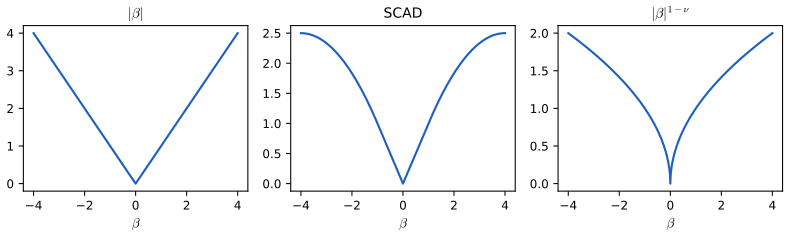
3.8.6 Pathwise Coordinate Optimization
pp. 92–93 An alternative to LARS is coordinate descent (Fu, 1998; Daubechies et al., 2004; Friedman et al., 2007; Wu and Lange, 2008): fix \(\lambda\) and minimise (3.52) over one coefficient at a time. With standardised predictors (unit norm), isolating \(\beta_j\),
\[ R(\tilde\bb(\lambda),\beta_j)=\frac12\sum_{i=1}^N\Big(y_i-\sum_{k\ne j}x_{ik}\tilde\beta_k(\lambda)-x_{ij}\beta_j\Big)^2+\lambda\sum_{k\ne j}|\tilde\beta_k(\lambda)|+\lambda|\beta_j|, \tag{3.83} \] \[ \tilde\beta_j(\lambda)\leftarrow S\Big(\sum_{i=1}^Nx_{ij}\big(y_i-\tilde y_i^{(j)}\big),\ \lambda\Big), \tag{3.84} \]with \(\tilde y_i^{(j)}=\sum_{k\ne j}x_{ik}\tilde\beta_k(\lambda)\) and \(S(t,\lambda)=\sign(t)(|t|-\lambda)_+\).
Result 3.30 (the coordinate update and its convergence) p. 93
(a) (3.84) is the exact minimiser of (3.83) in \(\beta_j\); for a column of squared norm \(n_j\ne1\) it is \(S(\bx_j^\T\br^{(j)},\lambda)/n_j\). (b) Cycling through the coordinates, every limit point of the iterates is a lasso solution, and the objective decreases monotonically to the minimum. (c) The pathwise strategy starts at \(\lambda_{\max}=\max_j|\bx_j^\T\by|\), where \(\hb=\mathbf{0}\), and warm-starts each smaller \(\lambda\) from the previous solution.
Proof
(a) As a function of \(\beta_j\), (3.83) is \(\frac{n_j}{2}\beta_j^2-\beta_j\bx_j^\T\br^{(j)}+\lambda|\beta_j|\)+const, with \(\br^{(j)}\) the partial residual: \(n_j/2\) times \(\big(\beta_j-\bx_j^\T\br^{(j)}/n_j\big)^2+\frac{2\lambda}{n_j}|\beta_j|\), whose minimiser is the soft-threshold of \(\bx_j^\T\br^{(j)}/n_j\) at \(\lambda/n_j\) (Result 3.17), i.e. \(S(\bx_j^\T\br^{(j)},\lambda)/n_j\). (b) Each update cannot increase \(R\), which is bounded below, so \(R\) converges. The smooth part is convex and the non-smooth part separable across coordinates; for such functions Tseng (2001) proves that every limit point of cyclic coordinate minimisation is a minimiser (the separability is essential: coordinatewise minimality then implies \(\mathbf{0}\in\partial R\), because \(\partial R\) is the product of the coordinate subdifferentials plus the gradient). The iterates are bounded since \(R\) is coercive, so limit points exist. (c) is the condition of Result 3.16. ∎
The speed comes from cheap updates (the inner product with the partial residual can be maintained as \(j\) varies) and from the fact that most updates leave \(\tilde\beta_j=0\). It gives solutions on a grid of \(\lambda\) rather than the exact path, and extends to the elastic net, the grouped lasso and any penalty that is a sum of functions of single coefficients (Friedman et al., 2010); the fused lasso (Section 18.4.2) needs modifications. The demonstrations and the code use LARS for paths and coordinate descent at fixed \(\lambda\), and they agree to \(10^{-9}\).
3.9 Computational Considerations
p. 93 Least squares is computed through the Cholesky decomposition of \(\bX^\T\bX\) (about \(p^3+Np^2/2\) operations) or the QR decomposition of \(\bX\) (about \(Np^2\)). Cholesky can be faster when \(N\gg p\), but QR is more stable (Lawson and Hanson, 1974): forming \(\bX^\T\bX\) squares the condition number, \(\kappa(\bX^\T\bX)=\kappa(\bX)^2\), so roughly twice as many digits are lost, whereas QR works with \(\bR\), which has the condition number of \(\bX\) itself (\(\bX^\T\bX=\bR^\T\bR\) and \(\bQ\) is an isometry). The lasso by LAR costs the same order as one least-squares fit with \(p\) predictors: each step updates a Cholesky or QR factor of the active Gram matrix by one row and column.
See also (companion courses): conditioning, the SVD and why a penalty helps; the SVD, the pseudo-inverse and numerical trouble.
Notes on the book
Points where the book's text or tables disagree with an exact computation, with the evidence. None changes the chapter's message.
1. Section 3.8.3: "if \(N<p\)" should read "if \(p<N\)" p. 89
The book says that for large \(t\) the lasso and the Dantzig selector "yield the least squares solution if \(N\lt p\). If \(p\ge N\), they both yield the least squares solution with minimum \(L_1\) norm". The two cases must be \(p\lt N\) (unique least-squares solution) and \(p\ge N\); as printed the first case contradicts the second. Result 3.28 proves the corrected statement, and the code confirms it on the prostate data (\(N=67>p=8\)).
2. Table 3.3: the ridge and PLS intercepts, and hence their test errors p. 63
The book prints the intercept 2.452 for ridge and PLS. That is the training mean of lpsa; it is the correct intercept only if the predictors are centred on the training set. They are not: with the standardisation that reproduces the LS column exactly (all 97 men), the intercept is \(\bar y-\bar{\bx}^\T\hb\), i.e. 2.464 for ridge and 2.467 for PLS. Evidence that the book used 2.452 with these coefficients: with intercept 2.452 our coefficients give test errors 0.492 (ridge) and 0.528 (PLS), exactly the book's entries; with the consistent intercepts they give 0.490 and 0.527.
3. Table 3.3: the lasso column is not on the lasso path of the standardisation used elsewhere p. 63
The book's lasso column has lbph = 0.002 and pgg45 empty. On the exact lasso path for the prostate data standardised as for the other columns, pgg45 enters before lbph (knots at \(s=0.367\) and 0.384; Figure 3.10), so no point of the path has lbph nonzero and pgg45 zero. With the predictors standardised on the training set instead, lbph does enter first (at \(s\approx0.375\), coefficients 0.562, 0.189, 0.002, 0.095 for lcavol, lweight, lbph, svi), so the book's lasso column was apparently computed with a different standardisation (and its lcavol 0.533 matches neither exactly). At \(s=0.36\) with the common standardisation we get 0.533, 0.176, 0.074 for lcavol, lweight, svi.
4. Figure 3.6 (and 3.16): the vertical axis
See the note under Figure 3.6: the plotted values cannot be \(\E\|\hat\bb(k)-\bb\|^2\) for the stated design (least squares alone gives 4.67, the plot about 0.66), and Figure 3.16's scale is likewise not reproducible from the stated setup.
5. Smaller points
- p. 51: the proof of the Gauss–Markov theorem "uses the triangle inequality"; it uses an orthogonal (Pythagorean) decomposition, Filling the gap 3.4.
- p. 72: the Laplace prior corresponding to the lasso has "\(\tau=1/\lambda\)"; this holds only for one value of the noise variance. In general \(\lambda=2\sigma^2/\tau\) for (3.53) (Filling the gap 3.8).
- p. 78: "after the \(k\)th step of the LAR procedure, the effective degrees of freedom of the fit vector is exactly \(k\)" is proved only under extra conditions on \(\bX\) (Efron et al., 2004); in general it is an approximation (our simulation: 1.03, 1.99, 2.96).
- Exercise 3.27(a) calls (3.89) "the Lagrange dual function"; (3.89) is the Lagrangian. The dual function is its infimum over the primal variables.
Exercises
All 30 exercises of Chapter 3 (pp. 94–99), restated in my own words, with complete solutions (hidden). Where an exercise needs computation, the method and the result of the Python code are given.
Exercise 3.1. Show that the F statistic (3.13) for dropping one coefficient equals the square of its Z-score (3.12).
Solution
Put the dropped input last and let \(\bz\) be it adjusted for all the others. Then \(\hat\beta_j=\langle\bz,\by\rangle/\|\bz\|^2\) and \(v_j=1/\|\bz\|^2\) (Result 3.8), and the big model's column space is the small one's plus the orthogonal direction \(\bz\), so \(\RSS_0-\RSS_1=\langle\bz,\by\rangle^2/\|\bz\|^2=\hat\beta_j^2/v_j\). With \(p_1-p_0=1\) the denominator of (3.13) is \(\hat\sigma^2\), so \(F=\hat\beta_j^2/(v_j\hat\sigma^2)=z_j^2\). Confirmed on the prostate data for all eight inputs (Filling the gap 3.2).
Exercise 3.2. For a cubic regression \(f(X)=\sum_{j=0}^3\beta_jX^j\), compare two 95% bands: (1) at each \(x_0\), the 95% interval for the linear function \(\ba^\T\bb\), \(\ba=(1,x_0,x_0^2,x_0^3)\); (2) the band generated by the confidence set (3.15). How do they differ, which is wider? Run a small simulation.
Solution
Both bands have the form \(\ba^\T\hb\pm c\,\hat\sigma\sqrt{\ba^\T(\bX^\T\bX)^{-1}\ba}\) (Filling the gap 3.3): \(c=z^{(0.975)}=1.96\) for (1) and \(c=\sqrt{{\chi^2_4}^{(0.95)}}=3.08\) for (2). So (2) is wider everywhere, by the factor 1.57. They answer different questions: (1) covers \(f(x_0)\) at any one \(x_0\) with probability about 95%; (2) covers the whole curve simultaneously with probability about 95%, since it is implied by the single event \(\bb\in C_\beta\).
Simulation (
band_simulation): \(N=40\) fixed inputs uniform on \((-1,1)\), \(f(x)=1+x-x^2+x^3\), \(\sigma=1\), 2000 replicates, a grid of 101 points. Average pointwise coverage: 0.938 for band (1) (slightly below 0.95 because the normal quantile is used with only 36 residual degrees of freedom; the \(t_{36}\) quantile would give about 0.95) and 0.995 for band (2). Simultaneous coverage of the whole curve: 0.701 for band (1), 0.966 for band (2). The pointwise band is the right tool for one \(x_0\); the wider band is needed for statements about the whole curve.Exercise 3.3. (a) Prove the Gauss–Markov theorem for \(\ba^\T\bb\). (b) Show that the covariance matrix of least squares is below (in the positive-semidefinite order) that of any other linear unbiased estimator of \(\bb\).
Solution
Both parts are proved in Filling the gap 3.4: unbiasedness means \(\bX^\T\bc=\ba\); writing \(\bc=\bc_0+\mathbf{d}\) with \(\bX^\T\mathbf{d}=\mathbf{0}\) gives \(\Var(\bc^\T\by)=\sigma^2(\|\bc_0\|^2+\|\mathbf{d}\|^2)\); for matrices, \(\Var(\tilde\bb)-\Var(\hb)=\sigma^2\mathbf{D}\mathbf{D}^\T\succeq0\). (Checked numerically with random unbiased alternatives.)
Exercise 3.4. Show how one pass of Gram–Schmidt (Algorithm 3.1) gives the whole least-squares coefficient vector, using the QR decomposition.
Solution
During the pass, store \(\hat\gamma_{kj}\), \(\|\bz_j\|\) and \(\hat\theta_j=\langle\bz_j,\by\rangle/\|\bz_j\|^2\). Since \(\bX=\bZ\mathbf{\Gamma}\) and \(\hat\by=\bZ\hat{\boldsymbol\theta}\), the coefficients solve \(\mathbf{\Gamma}\hb=\hat{\boldsymbol\theta}\), a unit upper-triangular system: \(\hat\beta_p=\hat\theta_p\), then \(\hat\beta_j=\hat\theta_j-\sum_{k>j}\hat\gamma_{jk}\hat\beta_k\) for \(j=p-1,\dots,0\). In QR terms, \(\bR\hb=\bQ^\T\by\) with \(\bR=\bD\mathbf{\Gamma}\) and \(\bQ^\T\by=\bD\hat{\boldsymbol\theta}\) (Result 3.9). The code's
gram_schmidtdoes exactly this and matches least squares to machine precision.Exercise 3.5. Show that ridge regression (3.41) is equivalent to
\[ \hb^c=\argmin_{\bb^c}\Big\{\sum_{i=1}^N\Big[y_i-\beta_0^c-\sum_{j=1}^p(x_{ij}-\bar x_j)\beta_j^c\Big]^2+\lambda\sum_{j=1}^p{\beta_j^c}^2\Big\}, \tag{3.85} \]give the correspondence between \(\bb^c\) and \(\bb\), characterise the solution, and show the same for the lasso.
Solution
\(\beta_j^c=\beta_j\) for \(j\ge1\) and \(\beta_0^c=\beta_0+\sum_j\bar x_j\beta_j\): a bijection under which the two criteria are identical, the penalty involving only the slopes. The solution has \(\hat\beta_0^c=\bar y\), slopes given by ridge (3.44) on the centred inputs and response, and \(\hat\beta_0=\bar y-\sum_j\bar x_j\hat\beta_j\). For the lasso replace \({\beta_j^c}^2\) by \(|\beta_j^c|\): the argument for \(\beta_0^c\) (its derivative is \(-2N(\bar y-\beta^c_0)\) whatever the slopes) is unchanged. Details: Filling the gap 3.6(a); checked numerically.
Exercise 3.6. With prior \(\bb\sim\N(\mathbf{0},\tau\bI)\) and \(\by\sim\N(\bX\bb,\sigma^2\bI)\), show the ridge estimate is the posterior mean and mode, and relate \(\lambda\) to \(\tau\) and \(\sigma^2\).
Solution
The log-posterior is \(-\frac{1}{2\sigma^2}\|\by-\bX\bb\|^2-\frac{1}{2\tau}\|\bb\|^2\)+const, a concave quadratic: completing the square, the posterior is \[ \N\big((\bX^\T\bX+\frac{\sigma^2}{\tau}\bI)^{-1}\bX^\T\by,\ \sigma^2(\bX^\T\bX+\frac{\sigma^2}{\tau}\bI)^{-1}\big) \]. Its mean and mode coincide and equal ridge with \(\lambda=\sigma^2/\tau\) (here \(\tau\) is a variance). See Result 3.15.
Exercise 3.7. With \(y_i\sim\N(\beta_0+x_i^\T\bb,\sigma^2)\) and independent \(\beta_j\sim\N(0,\tau^2)\), \(\sigma^2,\tau^2\) known, show that minus the log-posterior of \(\bb\) is proportional to \(\sum_i(y_i-\beta_0-\sum_jx_{ij}\beta_j)^2+\lambda\sum_j\beta_j^2\) with \(\lambda=\sigma^2/\tau^2\).
Solution
Up to additive constants, \[ -\log p(\bb\given\by)=\frac{1}{2\sigma^2}\sum_i(y_i-\beta_0-x_i^\T\bb)^2+\frac{1}{2\tau^2}\sum_j\beta_j^2=\frac{1}{2\sigma^2}\big[\sum_i(\cdot)^2+\frac{\sigma^2}{\tau^2}\sum_j\beta_j^2\big] \]. (With \(\beta_0\) given a flat prior; "proportional" must be read as "equal up to a positive factor and an additive constant".)
Exercise 3.8. Let \(\bX=\bQ\bR\) be the QR decomposition of the uncentred \(N\times(p+1)\) matrix (first column ones) and \(\tilde\bX=\bU\bD\bV^\T\) the SVD of the centred \(N\times p\) matrix. Show that \(\bQ_2\) (\(\bQ\) without its first column) and \(\bU\) span the same subspace. When are they equal up to sign flips?
Solution
The first column of \(\bQ\) is \(\bone/\sqrt N\). Since \(\bR\) is upper triangular and invertible, \(\col(\bQ)=\col(\bX)=\mathrm{span}(\bone)\oplus\col(\tilde\bX)\), an orthogonal sum because the centred columns are orthogonal to \(\bone\). The columns of \(\bQ_2\) are orthogonal to \(\bone\) and lie in \(\col(\bX)\), so \[ \col(\bQ_2)=\col(\bX)\ominus\mathrm{span}(\bone)=\col(\tilde\bX)=\col(\bU) \] (full rank). Explicitly, Gram–Schmidt's second step removes the mean, so \(\bQ_2\) is the Gram–Schmidt basis of the centred columns in their given order. The two bases coincide up to signs iff the Gram–Schmidt vectors are singular vectors: iff the centred columns are mutually orthogonal (then \(\bq_{j}=\tilde\bx_j/\|\tilde\bx_j\|\), and these are the \(\bu_j\)) and are ordered by decreasing norm (to match the ordering \(d_1\ge d_2\ge\dots\)); with equal norms the SVD is not unique and any orthonormal basis of a tied block is admissible. Checked numerically: the two projections \(\bQ_2\bQ_2^\T\) and \(\bU\bU^\T\) coincide on the prostate data.
Exercise 3.9. Given the QR decomposition of the current \(N\times q\) design \(\bX_1\) and its residual \(\br\), describe an efficient way to find which of the \(p-q\) candidate columns in \(\bX_2\) reduces the RSS most.
Solution
For each candidate compute \(\bz_j=\bx_j-\bQ(\bQ^\T\bx_j)\) (cost \(O(Nq)\)) and the reduction \(\langle\br,\bz_j\rangle^2/\|\bz_j\|^2\); pick the largest, then append \(\bz_j/\|\bz_j\|\) to \(\bQ\) and update \(\br\leftarrow\br-\bq\langle\bq,\br\rangle\). Better still, keep all candidates orthogonalised against the current \(\bQ\) and update them by one projection per step, \(O(N(p-q))\) per step. Proof: Result 3.11. The code's
forward_stepwiseis this algorithm.Exercise 3.10. From the full fit with its standard errors and Z-scores, which variable, if dropped, increases the RSS least?
Solution
The one with the smallest \(|z_j|\): the increase is \(z_j^2\hat\sigma^2\) (Result 3.12). For the prostate data (Table 3.2) that is
gleason(\(z=-0.15\)), increase \(0.15^2\times0.507=0.011\), matching the RSS 29.43 of the best 7-variable model in Figure 3.5 against 29.43 for all eight.Exercise 3.11. Show that the solution of the multivariate problem (3.40) is (3.39). What if the covariance \(\mathbf{\Sigma}_i\) differs between observations?
Solution
See Result 3.10: the gradient \(-2\bX^\T(\bY-\bX\bB)\mathbf{\Sigma}^{-1}\) vanishes iff \(\bX^\T(\bY-\bX\bB)=\mathbf{0}\). With observation-specific \(\mathbf{\Sigma}_i\), the normal equations \(\sum_i x_ix_i^\T\bB\mathbf{\Sigma}_i^{-1}=\sum_ix_iy_i^\T\mathbf{\Sigma}_i^{-1}\) couple the columns of \(\bB\): in vectorised form \[ \big(\sum_i\mathbf{\Sigma}_i^{-1}\otimes x_ix_i^\T\big)\mathrm{vec}(\bB)=\sum_i\mathrm{vec}(x_iy_i^\T\mathbf{\Sigma}_i^{-1}) \], a generalised least-squares problem that must be solved jointly (it decouples only if all \(\mathbf{\Sigma}_i\) are proportional to one matrix).
Exercise 3.12. Show that ridge regression is least squares on the centred data augmented with \(p\) rows \(\sqrt\lambda\bI\) and \(p\) zero responses.
Solution
\(\tilde\bX^\T\tilde\bX=\bX^\T\bX+\lambda\bI\) and \(\tilde\bX^\T\tilde\by=\bX^\T\by\), so the normal equations of the augmented problem are (3.44): Filling the gap 3.6(e). Equivalently, the augmented RSS is \(\|\by-\bX\bb\|^2+\sum_j(0-\sqrt\lambda\beta_j)^2\), the ridge criterion. The \(p\) artificial cases, each saying "\(\beta_j\) is about zero", are an instance of the hints of Abu-Mostafa (1995).
Exercise 3.13. Derive (3.62) and show \(\hb^{\rm pcr}(p)=\hb^{\rm ls}\).
Solution
Result 3.21: \(\bz_m=\bX\bv_m\), so \(\sum_m\hat\theta_m\bz_m=\bX\sum_m\hat\theta_m\bv_m\); with \(M=p\), \(\sum_m\bv_m\bu_m^\T\by/d_m=\bV\bD^{-1}\bU^\T\by=\hb^{\rm ls}\). Checked numerically.
Exercise 3.14. Show that with orthogonal inputs PLS stops after \(m=1\): the later \(\hat\varphi_{mj}\) are zero.
Solution
Result 3.22(c): with \(\bX^\T\bX=c\bI\) (orthogonal, standardised), \(\hat\by^{(1)}\) is already the least-squares fit, so the residual is orthogonal to every input and \(\hat\varphi_{2j}=\langle\bx_j,\by-\hat\by^{(1)}\rangle=0\); then \(\bz_2=\mathbf{0}\) and nothing changes. (If the orthogonal inputs had unequal norms, PLS would need more steps: the first direction would weight them by \(\|\bx_j\|^2\) as well; standardisation matters.)
Exercise 3.15. Verify (3.64) and hence show that the PLS directions compromise between the ordinary regression coefficient and the principal component directions.
Solution
Result 3.22(b): the criterion equals \((\ba^\T\bX^\T\by)^2/(N\|\by\|^2)\), maximised over unit \(\ba\) at \(\ba\propto\bX^\T\by\) (checked numerically against 3000 random directions). Writing \(\bX^\T\by=\sum_jd_j(\bu_j^\T\by)\bv_j\) shows the compromise: the PLS direction weights the principal directions \(\bv_j\) by \(d_j\) (variance) times \(\bu_j^\T\by\) (correlation with \(\by\)); the principal component direction uses variance only (\(\bv_1\)), while the least-squares coefficient \(\sum_jd_j^{-1}(\bu_j^\T\by)\bv_j\) weights by correlation divided by \(d_j\). The variance factor \(\Var(\bX\ba)\) favours high-variance directions, the \(\Corr^2\) factor directions that track \(\by\).
Exercise 3.16. Derive the entries of Table 3.4.
Solution
Result 3.17: with orthonormal inputs the criteria separate into \((\hat\beta_j-\beta_j)^2\) plus the penalty, giving hard thresholding (best subset), \(\hat\beta_j/(1+\lambda)\) (ridge) and soft thresholding at \(\lambda\) (lasso, with the \(\frac12\) of (3.52)). Checked numerically on a random orthonormal design.
Exercise 3.17. Repeat the analysis of Table 3.3 on the spam data of Chapter 1.
Solution
Method (
spam_table). The 0/1 response (spam or not) is regressed on the 57 inputs, transformed by \(\log(x+0.1)\) (the word and character frequencies are very skewed) and standardised; the book's split gives 3065 training and 1536 test emails. Each complexity is chosen by tenfold CV with the one-SE rule. Best subset over \(2^{57}\) models is out of reach, so forward stepwise takes its place. We report the test mean squared error and the misclassification rate of the rule \(\hat y>0.5\).Method Chosen Nonzero Test MSE (SE) Misclassification Least squares 57 inputs 57 0.0727 (0.0032) 6.5% Forward stepwise 21 inputs 21 0.0748 (0.0032) 7.1% Ridge df = 36 57 0.0748 (0.0031) 7.1% Lasso \(s=0.70\) 32 0.0744 (0.0032) 7.0% PCR 39 directions 57 0.0750 (0.0033) 7.8% PLS 4 directions 57 0.0739 (0.0033) 6.6% Conclusions. With \(N=3065\) cases for 57 inputs there is little variance to remove, so shrinkage and selection do not beat least squares on test error (all within one standard error); their value here is parsimony: the lasso uses 32 inputs and forward stepwise 21 at essentially the same accuracy. A linear probability model is not the natural tool for a 0/1 response; logistic regression (Chapter 4) and the additive model (Chapter 9) reach lower error rates.
Exercise 3.18. Read about conjugate gradient algorithms and establish a connection with partial least squares.
Solution
Result 3.23 and Filling the gap 3.12: \(\hb^{\rm pls}(m)\) minimises the RSS over the Krylov subspace \(\mathcal{K}_m(\bX^\T\bX,\bX^\T\by)\), which is exactly the \(m\)th conjugate gradient iterate for \(\bX^\T\bX\bb=\bX^\T\by\) started at zero (Wold et al., 1984; Phatak and de Hoog, 2002). The code checks that the CG iterates equal the PLS coefficients for \(m=1,\dots,8\) on the prostate data. Consequences: PLS reaches least squares in at most as many steps as \(\bX^\T\bX\) has distinct eigenvalues, and its shrinkage factors are the residual polynomials of CG.
Exercise 3.19. Show that \(\|\hb^{\rm ridge}\|\) increases as \(\lambda\to0\). Does the same hold for the lasso and for PLS (with the step number as tuning parameter)?
Solution
Ridge. \(\|\hb_\lambda\|^2=\sum_j\frac{d_j^2(\bu_j^\T\by)^2}{(d_j^2+\lambda)^2}\), each term non-increasing in \(\lambda\), strictly decreasing if \(d_j\bu_j^\T\by\ne0\). So the norm increases as \(\lambda\downarrow0\).
Lasso. The \(L_1\) norm \(\|\hb_\lambda\|_1\) is non-increasing in \(\lambda\): for \(\lambda_1\lt \lambda_2\), optimality of each solution gives \(\RSS_1+\lambda_1\ell_1\le\RSS_2+\lambda_1\ell_2\) and \(\RSS_2+\lambda_2\ell_2\le\RSS_1+\lambda_2\ell_1\) (\(\ell=\|\cdot\|_1\)); adding, \((\lambda_2-\lambda_1)(\ell_2-\ell_1)\le0\). The Euclidean norm need not be monotone: in a simulated example with three correlated inputs the lasso path has the knots
\[ (0,0,0)\to(-5.28,0,0)\to(-4.74,-0.81,0)\to(-4.20,-1.67,0.42) \]with Euclidean norms 0, 5.28, 4.81, 4.53, decreasing as \(\lambda\to0\) after the first knot (the \(L_1\) norms are 0, 5.28, 5.55, 6.28).
PLS. Yes: \(\|\hb^{\rm pls}(m)\|\) is non-decreasing in \(m\) (de Jong, 1995). Since \(\hb^{\rm pls}(m)\) are CG iterates from 0, this is the classical fact that CG iterates increase in norm (Hestenes and Stiefel, 1952; Steihaug, 1983). On the prostate data the norms are confirmed to be non-decreasing. Note that this does not mean every principal-component coordinate grows: some are inflated beyond least squares and then come back (Result 3.23).
Exercise 3.20. Show that the leading canonical pair solves
\[ \max_{\substack{\bu^\T(\bY^\T\bY)\bu=1\\ \bv^\T(\bX^\T\bX)\bv=1}}\bu^\T(\bY^\T\bX)\bv, \tag{3.86} \]a generalised SVD problem, with solution \(\bu_1=(\bY^\T\bY)^{-1/2}\bu_1^*\), \(\bv_1=(\bX^\T\bX)^{-1/2}\bv_1^*\) from the leading singular vectors of
\[ (\bY^\T\bY)^{-1/2}(\bY^\T\bX)(\bX^\T\bX)^{-1/2}=\bU^*\bD^*\bV^{*\T}, \tag{3.87} \]and that the whole sequence \(\bu_m,\bv_m\), \(m=1,\dots,\min(K,p)\), comes from (3.87).
Solution
Filling the gap 3.13(a). The correlation of \(\bY\bu\) and \(\bX\bv\) is scale-free, so it can be maximised under the two normalisations, where it equals \(\bu^\T\bY^\T\bX\bv\); whitening turns (3.86) into the maximisation of \(\ba^\T\mathbf{K}\mathbf{b}\) over unit vectors, solved by the top singular pair. The \(m\)th canonical pair must be uncorrelated with the earlier ones, i.e. \(\ba\perp\ba_1..\ba_{m-1}\), \(\mathbf{b}\perp\mathbf{b}_1..\mathbf{b}_{m-1}\), which gives the \(m\)th singular pair; the canonical correlations are the singular values \(d^*_m\). Checked numerically.
Exercise 3.21. Show that reduced-rank regression (3.68) with \(\mathbf{\Sigma}=\bY^\T\bY/N\) has solution (3.69). (Hint: transform to \(\bY^*=\bY\mathbf{\Sigma}^{-1/2}\); show \(\bU_m=\mathbf{\Sigma}^{-1/2}\bU^*_m\) and \(\bU_m^-=\bU_m^{*\T}\mathbf{\Sigma}^{1/2}\).)
Solution
Filling the gap 3.13(b): after whitening the criterion is a Frobenius norm, which splits by Pythagoras into a constant and \(\|\bH\bY^*-\bX\bB^*\|_F^2\); Eckart–Young gives the rank-\(m\) truncation of \(\bH\bY^*\) on its top right singular vectors, which are \(\bU^*_m\). Mapping back gives \(\hat\bB\mathbf{\Sigma}^{-1/2}\bU^*_m\bU^{*\T}_m\mathbf{\Sigma}^{1/2}\). Checked numerically against a direct minimisation.
Exercise 3.22. Show that the solution of Exercise 3.21 is unchanged if \(\mathbf{\Sigma}\) is estimated by \((\bY-\bX\hat\bB)^\T(\bY-\bX\hat\bB)/(N-pK)\).
Solution
Filling the gap 3.13(c): with \(\mathbf{F}=\bY^\T\bH\bY\) and \(\mathbf{E}^\T\mathbf{E}=\bY^\T\bY-\mathbf{F}\), the generalised eigenproblems \(\mathbf{F}\ba=\nu\bY^\T\bY\ba\) and \(\mathbf{F}\ba=\mu\mathbf{E}^\T\mathbf{E}\ba\) have the same eigenvectors with \(\mu=\nu/(1-\nu)\) increasing in \(\nu\), so the same leading \(m\)-dimensional subspace and the same projection \(\bU_m\bU_m^-\) (the constant \(N-pK\) cancels). Checked numerically.
Exercise 3.23. All variables and the response have mean 0 and standard deviation 1, and every input has the same absolute correlation with the response, \(\frac1N|\langle\bx_j,\by\rangle|=\lambda\). Let \(\hb\) be the least-squares coefficient, \(\bu(\alpha)=\alpha\bX\hb\) for \(\alpha\in[0,1]\), and RSS the full least-squares residual sum of squares. (a) Show \(\frac1N|\langle\bx_j,\by-\bu(\alpha)\rangle|=(1-\alpha)\lambda\). (b) Show the correlations equal \(\lambda(\alpha)=\frac{(1-\alpha)}{\sqrt{(1-\alpha)^2+\frac{\alpha(2-\alpha)}{N}\RSS}}\lambda\), decreasing to 0. (c) Deduce that LAR keeps the correlations tied and decreasing.
Solution
(a) \(\bX^\T(\by-\bX\hb)=\mathbf{0}\), so \(\bx_j^\T\bu(\alpha)=\alpha\bx_j^\T\by\) and \(\bx_j^\T(\by-\bu(\alpha))=(1-\alpha)\bx_j^\T\by\).
(b) The residual \(\by-\bu=(\by-\hat\by)+(1-\alpha)\hat\by\) is an orthogonal sum, so \[ \|\by-\bu\|^2=\RSS+(1-\alpha)^2(N-\RSS) \], using \(\|\by\|^2=N\) and \(\|\hat\by\|^2=N-\RSS\). This equals \(N\big[(1-\alpha)^2+\frac{\alpha(2-\alpha)}{N}\RSS\big]\). The residual has mean zero, so its standard deviation is \(\sqrt{\|\by-\bu\|^2/N}\), and dividing (a) by it (the inputs have standard deviation 1) gives \(\lambda(\alpha)\). Its derivative in \(\alpha\) has the sign of \(-\RSS/N-(1-\alpha)\cdot0\le0\): writing \(g=(1-\alpha)^2\), \(\lambda(\alpha)/\lambda=\sqrt{g/(g+(1-g)\RSS/N)}\), increasing in \(g\), and \(g\) decreases from 1 to 0; so \(\lambda(\alpha)\) decreases from \(\lambda\) to 0.
(c) In a LAR step the active inputs are tied and the step moves the fit towards the least-squares fit on the active set, i.e. exactly \(\bu(\alpha)\) for the problem restricted to \(\bX_\mathcal{A}\) with response the current residual; (a)–(b) apply and the active correlations stay tied and decrease, as claimed around (3.55). The general (not equal-correlation) case is Result 3.18(a). Formula (b) is confirmed numerically.
Exercise 3.24. Show that the LAR direction makes an equal angle with each active predictor.
Solution
\(\bX_\mathcal{A}^\T\bu_k=C\bs_\mathcal{A}\), so with unit-norm inputs \(|\cos\angle(\bx_j,\bu_k)|=C/\|\bu_k\|\) for all \(j\in\mathcal{A}\): Result 3.18(b). The LARS demonstration prints these cosines at every step.
Exercise 3.25. At the start of step \(k\) of LAR, find the next variable to enter and the value of \(\alpha\) at which it enters.
Solution
With \(c_\ell=\bx_\ell^\T\br_k\), \(C=\max_j|c_j|\) and \(a_\ell=\bx_\ell^\T\bu_k\), the next variable is the inactive \(\ell\) minimising the smallest positive root of \(c_\ell-\alpha a_\ell=\pm(1-\alpha)C\), i.e. of \(\frac{C-c_\ell}{C-a_\ell}\) and \(\frac{C+c_\ell}{C+a_\ell}\); \(\alpha\) is that minimum (in the book's parametrisation of (3.55), where \(\alpha=1\) is the active least-squares fit). See Result 3.18(c) and Efron et al. (2004), Section 2.
Exercise 3.26. Forward stepwise enters the variable that most reduces the RSS; LAR the one most correlated with the residual. Show these can differ. (Hint: with \(\bx_{j\cdot\mathcal{A}}\) the \(j\)th variable adjusted for the current model, forward stepwise maximises \(|\Corr(\bx_{j\cdot\mathcal{A}},\br)|\).)
Solution
By Result 3.11 the RSS reduction is \(\langle\br,\bz_j\rangle^2/\|\bz_j\|^2=\|\br\|^2\Corr^2(\bz_j,\br)\) with \(\bz_j=\bx_{j\cdot\mathcal{A}}\), and \(\langle\br,\bz_j\rangle=\langle\br,\bx_j\rangle\) since \(\br\perp\col(\bX_\mathcal{A})\). So forward stepwise maximises \(|\langle\bx_j,\br\rangle|/\|\bz_j\|\), LAR maximises \(|\langle\bx_j,\br\rangle|\) (unit-norm inputs). They differ when an input with a slightly smaller inner product is much more correlated with the current model (short \(\bz_j\)), which divides its inner product by a small norm. Moreover LAR's residual is not the forward-stepwise residual after the first step. The code finds an explicit example (four random inputs, \(N=30\)) where both enter the same first variable but different second variables.
Exercise 3.27. For the lasso \(L(\bb)+\lambda\sum_j|\beta_j|\) with \(L(\bb)=\frac12\sum_i(y_i-\sum_jx_{ij}\beta_j)^2\):
\[ L(\bb)+\lambda\sum_j|\beta_j| \tag{3.88} \](a) with \(\beta_j=\beta_j^+-\beta_j^-\), \(\beta_j^\pm\ge0\), write the Lagrangian
\[ L(\bb)+\lambda\sum_j(\beta_j^++\beta_j^-)-\sum_j\lambda_j^+\beta_j^+-\sum_j\lambda_j^-\beta_j^- \tag{3.89} \]and the KKT conditions \(\nabla L(\bb)_j+\lambda-\lambda_j^+=0\), \(-\nabla L(\bb)_j+\lambda-\lambda_j^-=0\), \(\lambda_j^+\beta_j^+=0\), \(\lambda_j^-\beta_j^-=0\); (b) show \(|\nabla L(\bb)_j|\le\lambda\) and the three scenarios, so that an active \(\beta_j\) has \(\nabla L_j=-\lambda\sign\beta_j\), and relate \(\lambda\) to correlations; (c) show that with a fixed active set for \(\lambda_0\ge\lambda\ge\lambda_1\), \(\hb(\lambda)=\hb(\lambda_0)-(\lambda-\lambda_0)\boldsymbol\gamma_0\) (3.90).
Solution
(a) The split problem minimises the smooth convex \(L(\bb^+-\bb^-)+\lambda\bone^\T(\bb^++\bb^-)\) over \(\bb^\pm\ge\mathbf{0}\); (3.89) is its Lagrangian (not the dual function, which would be its infimum over \(\bb^\pm\)). Stationarity in \(\beta_j^+\) and \(\beta_j^-\) (\(\partial L/\partial\beta_j^\pm=\pm\nabla L_j\)) gives the first two equations, complementary slackness the last two, with \(\lambda_j^\pm\ge0\). The constraints are linear, so the KKT conditions are necessary and sufficient.
(b) From the first two, \(\lambda_j^+=\nabla L_j+\lambda\ge0\) and \(\lambda_j^-=\lambda-\nabla L_j\ge0\): \(|\nabla L_j|\le\lambda\). If \(\lambda=0\), \(\nabla L=\mathbf{0}\) (least squares). If \(\beta_j^+>0\) then \(\lambda_j^+=0\), so \(\nabla L_j=-\lambda\lt 0\), hence \(\lambda_j^-=2\lambda>0\) and \(\beta_j^-=0\). Symmetrically \(\beta_j^->0\) forces \(\nabla L_j=\lambda\), \(\beta_j^+=0\). So an active coefficient has \(\nabla L_j=-\lambda\sign\beta_j\). Since \(\nabla L_j=-\bx_j^\T\br\), this says \(\bx_j^\T\br=\lambda\sign\beta_j\): with standardised inputs, \(\lambda\) is \(N\) times the common absolute covariance, i.e. proportional to the common absolute correlation of the active inputs with the residual, and inactive inputs have smaller absolute correlation. This is (3.58)–(3.59).
(c) On the interval the active set \(\mathcal{A}\) and signs \(\bs\) are fixed, and \(\bX_\mathcal{A}^\T(\by-\bX_\mathcal{A}\bb_\mathcal{A})=\lambda\bs\) gives \(\hb_\mathcal{A}(\lambda)=(\bX_\mathcal{A}^\T\bX_\mathcal{A})^{-1}(\bX_\mathcal{A}^\T\by-\lambda\bs)\). Subtracting the same expression at \(\lambda_0\), \(\hb(\lambda)=\hb(\lambda_0)-(\lambda-\lambda_0)\boldsymbol\gamma_0\) with \(\boldsymbol\gamma_{0,\mathcal{A}}=(\bX_\mathcal{A}^\T\bX_\mathcal{A})^{-1}\bs\) and zeros elsewhere: the path is linear. Confirmed numerically at the midpoint between two knots.
Exercise 3.28. For a given \(t\) in (3.51), the lasso coefficient of \(X_j\) is \(a\). Add an exact copy \(X_j^*=X_j\). Describe the set of solutions for \(\hat\beta_j,\hat\beta_j^*\) with the same \(t\).
Solution
The fit depends only on \(\beta_j+\beta_j^*\), and \(|\beta_j|+|\beta_j^*|\ge|\beta_j+\beta_j^*|\), with equality iff the two have the same sign (or one is zero). Any solution of the augmented problem therefore has \(\beta_j+\beta_j^*\) equal to a solution of the original problem with the same budget (a split with opposite signs would waste budget that could reduce the RSS, unless the constraint is slack). So the solutions are \(\{(\hat\beta_j,\hat\beta_j^*):\hat\beta_j+\hat\beta_j^*=a,\ \hat\beta_j\hat\beta_j^*\ge0\}\), the segment from \((a,0)\) to \((0,a)\), with all other coefficients unchanged: the lasso does not determine how the weight is shared. Checked numerically (coordinate descent puts it all on one copy). By contrast ridge splits it equally (Exercise 3.29), and the elastic net too.
Exercise 3.29. Ridge with parameter \(\lambda\) on one variable \(X\) gives coefficient \(a\). Include an exact copy \(X^*=X\) and refit: show both coefficients are equal and find them. More generally, with \(m\) copies of a variable all coefficients are equal.
Solution
With one variable, \(a=\bx^\T\by/(\bx^\T\bx+\lambda)\). With \(m\) copies, the fit depends on \(S=\sum_k\beta_k\) only, and for fixed \(S\) the penalty \(\sum_k\beta_k^2\) is minimised uniquely (strict convexity) at \(\beta_k=S/m\). So the coefficients are equal, \(\beta\), and minimise \(\|\by-m\beta\bx\|^2+m\lambda\beta^2\): \(\beta=\bx^\T\by/(m\bx^\T\bx+\lambda)\). For \(m=2\), \(\beta=\bx^\T\by/(2\bx^\T\bx+\lambda)\); the total \(2\beta\) is slightly more than \(a\) (shrinkage is effectively halved). The same argument applies to copies of \(X_j\) inside a larger ridge regression: swapping two copies' coefficients leaves the criterion unchanged, and the unique minimiser must be symmetric. Checked for \(m=1,2,3,5\).
Exercise 3.30. Turn the elastic-net problem
\[ \min_{\bb}\|\by-\bX\bb\|^2+\lambda\big[\alpha\|\bb\|_2^2+(1-\alpha)\|\bb\|_1\big] \tag{3.91} \]into a lasso problem on augmented data.
Solution
Augment as in Exercise 3.12 with the ridge part: \(\tilde\bX=\binom{\bX}{\sqrt{\lambda\alpha}\bI_p}\), \(\tilde\by=\binom{\by}{\mathbf{0}}\). Then \(\|\tilde\by-\tilde\bX\bb\|^2=\|\by-\bX\bb\|^2+\lambda\alpha\|\bb\|^2\), so (3.91) is the lasso \(\|\tilde\by-\tilde\bX\bb\|^2+\lambda(1-\alpha)\|\bb\|_1\) (in the form (3.52) with the factor \(\frac12\): penalty \(\frac{\lambda(1-\alpha)}{2}\)). The augmented matrix has full column rank for \(\alpha>0\), so the solution is unique, even when \(p>N\) (Zou and Hastie, 2005). The code solves the augmented lasso and checks the elastic-net optimality conditions to \(10^{-7}\).
Demonstrations for this chapter
Each demonstration runs in the browser on the book's prostate data (or a fixed simulated data set exported by the Python code) and links back to these notes. The ▶ Demo boxes above open them already set to the case under discussion.
| Demonstration | What you can see | Sections and results |
|---|---|---|
| Ridge and lasso on the prostate data | Coefficient profiles against df(λ) or \(s\); ridge shrinkage factors on the principal components; the lasso's inner products against \(\lambda\); training and test error; coefficients against least squares. Presets: 1 ridge df 5; 2 lasso \(s=0.36\); 3 ridge df 2; 4 one active variable; 5 back to least squares. | 3.4.1, 3.4.2; Results 3.13, 3.16 |
| Least angle regression step by step | The absolute correlations and the coefficients against \(L_1\) arc length, knot by knot, for LAR, the lasso modification and FSε; the equal-angle cosines and step lengths. Presets: 1 first step; 2 LAR = lasso on the prostate data; 3 a coefficient crosses zero; 4 the drop; 5 FSε. | 3.4.4, 3.8.1; Results 3.18, 3.19, 3.26 |
| PCR, PLS and ridge | Shrinkage factors of the three methods on each principal component (PLS factors above 1 in gold); test error against complexity; the two-input paths of Figure 3.18 for any \(\rho\). Presets: 1 PCR \(M=7\); 2 PLS \(M=2\); 3 PLS \(M=3\); 4 \(\rho=0.5\); 5 \(\rho=-0.5\). | 3.5, 3.6; Results 3.21, 3.23, 3.24 |
Related demonstrations in the companion courses: L1 versus L2 regularisation (paths on simulated sparse data and the \(L_q\) geometry) and bias and variance. The Python code that produces every figure and table of this page is code/ch03_linear_regression.py (see the code index).
References
- Hastie, T., Tibshirani, R. and Friedman, J. (2009). The Elements of Statistical Learning: Data Mining, Inference, and Prediction, 2nd edition. Springer, New York. Chapter 3, pp. 43–99. hastie.su.domains/ElemStatLearn.
- Bickel, P. J., Ritov, Y. and Tsybakov, A. B. (2009). Simultaneous analysis of lasso and Dantzig selector. Annals of Statistics, 37(4), 1705–1732.
- Breiman, L. and Friedman, J. H. (1997). Predicting multivariate responses in multiple linear regression (with discussion). Journal of the Royal Statistical Society B, 59(1), 3–54.
- Bühlmann, P. and Hothorn, T. (2007). Boosting algorithms: regularization, prediction and model fitting. Statistical Science, 22(4), 477–505.
- Candès, E. and Tao, T. (2007). The Dantzig selector: statistical estimation when p is much larger than n. Annals of Statistics, 35(6), 2313–2351.
- de Jong, S. (1995). PLS shrinks. Journal of Chemometrics, 9(4), 323–326.
- Efron, B., Hastie, T., Johnstone, I. and Tibshirani, R. (2004). Least angle regression (with discussion). Annals of Statistics, 32(2), 407–499.
- Fan, J. and Li, R. (2001). Variable selection via nonconcave penalized likelihood and its oracle properties. Journal of the American Statistical Association, 96, 1348–1360.
- Frank, I. E. and Friedman, J. H. (1993). A statistical view of some chemometrics regression tools. Technometrics, 35(2), 109–135.
- Friedman, J., Hastie, T., Höfling, H. and Tibshirani, R. (2007). Pathwise coordinate optimization. Annals of Applied Statistics, 1(2), 302–332.
- Friedman, J., Hastie, T. and Tibshirani, R. (2010). Regularization paths for generalized linear models via coordinate descent. Journal of Statistical Software, 33(1), 1–22.
- Furnival, G. M. and Wilson, R. W. (1974). Regressions by leaps and bounds. Technometrics, 16(4), 499–511.
- Hastie, T., Taylor, J., Tibshirani, R. and Walther, G. (2007). Forward stagewise regression and the monotone lasso. Electronic Journal of Statistics, 1, 1–29.
- Hestenes, M. R. and Stiefel, E. (1952). Methods of conjugate gradients for solving linear systems. Journal of Research of the National Bureau of Standards, 49(6), 409–436.
- Hoerl, A. E. and Kennard, R. W. (1970). Ridge regression: biased estimation for nonorthogonal problems. Technometrics, 12(1), 55–67.
- Izenman, A. J. (1975). Reduced-rank regression for the multivariate linear model. Journal of Multivariate Analysis, 5(2), 248–264.
- Lawson, C. L. and Hanson, R. J. (1974). Solving Least Squares Problems. Prentice-Hall, Englewood Cliffs.
- Meinshausen, N. (2007). Relaxed lasso. Computational Statistics and Data Analysis, 52(1), 374–393.
- Phatak, A. and de Hoog, F. (2002). Exploiting the connection between PLS, Lanczos methods and conjugate gradients. Journal of Chemometrics, 16(7), 361–367.
- Rosset, S. and Zhu, J. (2007). Piecewise linear regularized solution paths. Annals of Statistics, 35(3), 1012–1030.
- Stamey, T., Kabalin, J., McNeal, J., Johnstone, I., Freiha, F., Redwine, E. and Yang, N. (1989). Prostate specific antigen in the diagnosis and treatment of adenocarcinoma of the prostate II: radical prostatectomy treated patients. Journal of Urology, 141(5), 1076–1083.
- Stone, M. and Brooks, R. J. (1990). Continuum regression: cross-validated sequentially constructed prediction embracing ordinary least squares, partial least squares and principal components regression. Journal of the Royal Statistical Society B, 52(2), 237–269.
- Tibshirani, R. (1996). Regression shrinkage and selection via the lasso. Journal of the Royal Statistical Society B, 58(1), 267–288.
- Tibshirani, R. J. (2013). The lasso problem and uniqueness. Electronic Journal of Statistics, 7, 1456–1490.
- Tseng, P. (2001). Convergence of a block coordinate descent method for nondifferentiable minimization. Journal of Optimization Theory and Applications, 109(3), 475–494.
- Yuan, M. and Lin, Y. (2006). Model selection and estimation in regression with grouped variables. Journal of the Royal Statistical Society B, 68(1), 49–67.
- Zou, H. (2006). The adaptive lasso and its oracle properties. Journal of the American Statistical Association, 101, 1418–1429.
- Zou, H. and Hastie, T. (2005). Regularization and variable selection via the elastic net. Journal of the Royal Statistical Society B, 67(2), 301–320.
- Zou, H., Hastie, T. and Tibshirani, R. (2007). On the "degrees of freedom" of the lasso. Annals of Statistics, 35(5), 2173–2192.
The numerical statements in the text (the tables, the sampling distributions, the Gauss–Markov inequality, the identities of the SVD, QR and Krylov forms, the lasso and LAR paths against independent implementations, the degrees-of-freedom formulas, and the exercise results) were confirmed numerically.