Neural Networks for Images
An image is a grid of numbers whose meaning does not change when an object moves a few pixels: a dense layer ignores that structure, a convolutional layer builds it in. A convolution applies the same small filter at every position, which cuts the number of weights by orders of magnitude and makes the layer commute with translations. This chapter takes the idea from the arithmetic of a single layer (padding, stride, dilation, channels, pooling) through normalisation layers, the classical architectures (LeNet, AlexNet, Inception, ResNet, DenseNet), other kinds of convolution (dilated, transposed, depthwise separable) and other vision tasks (tagging, detection, segmentation), to the last section of the chapter, where a trained classifier is run backwards to generate images (class-conditional synthesis with Gaussian and total-variation priors, activation maximisation, DeepDream and neural style transfer). The notes prove what the book leaves as "one can show", count parameters exactly, and check the formulas on small simulated problems and on digits.
Ch. 1 Introduction Ch. 2 Univariate probability Ch. 3 Multivariate probability Ch. 4 Statistics Ch. 5 Decision theory Ch. 6 Information theory Ch. 7 Linear algebra Ch. 8 Optimisation Ch. 9 Discriminant analysis Ch. 10 Logistic regression Ch. 11 Linear regression Ch. 12 GLMs Ch. 13 Networks for tabular data Ch. 14 Networks for images Ch. 15 Networks for sequences Ch. 16 Exemplar-based methods Ch. 17 Kernel methods Ch. 18 Trees and boosting Ch. 19 Fewer labels Ch. 20 Dimensionality reduction Ch. 21 Clustering Ch. 22 Recommender systems Ch. 23 Graph embeddings
How to read these notes
They follow the book. Sections carry the book's numbers (14.2.1.3, 14.4.2, ...) and equations the book numbers keep their numbers, e.g. \((14.8)\); equations without a number are steps the book skips. The book marks Sections 14.4, 14.5 and 14.6 as optional (stars); they are covered here, more briefly where the material is descriptive and in full where there is mathematics to fill in.
Filling the gaps. Wherever the book writes "one can show", leaves a step out, or quotes a result from the literature, an orange Filling the gap box gives the full argument. Proofs start hidden: open one with its bar, or use the buttons below.
Figures and demonstrations. Every computed figure is reproduced by the Python code. Figures 14.2, 14.4, 14.10, 14.13, 14.15, 14.18 to 14.22, 14.27a, 14.28 to 14.32, 14.39 and 14.40 are hand-drawn diagrams or photographs and are not reproduced; the layer sizes and parameter counts that the diagrams carry are computed instead. The book's networks (AlexNet, Inception, ImageNet classifiers) and photographs are not available offline, so the figures about images use the two photographs shipped with scikit-learn, MNIST digits, simulated images and a small CNN trained here; the captions say so. The ▶ Demo boxes open an interactive demonstration set to the case being discussed.
Main reference
K. P. Murphy, Probabilistic Machine Learning: An Introduction, MIT Press (2022), Chapter 14, pages 467–501 (book page: probml.github.io/pml-book/book1.html). Section, equation, figure and exercise numbers below refer to this book. The explanations, derivations, figures and code are my own.
Companion courses
Convolutional networks and their training are developed, in other notation, elsewhere on this site. Where a result is proved in full there, these notes give the statement and a short sketch and link to it.
- Foundations of Deep Learning (Bishop and Bishop): Chapter 10 on convolutional networks (10.2 convolutional filters, 10.3 visualizing trained CNNs, 10.4 object detection, 10.5 image segmentation, 10.6 style transfer), 7.4 normalization, 9.5 residual connections, Chapter 8 on backpropagation, 14.3.3 Langevin dynamics.
- Bayesian and Probabilistic Machine Learning (Bishop): 5.5.3 invariances, 5.5.6 convolutional networks, 5.3 error backpropagation.
- Introduction to Statistical Learning: 10.3 convolutional neural networks (convolution and pooling layers, architecture, data augmentation, pretrained classifiers).
- Elements of Statistical Learning: 11.5 some issues in training neural networks (starting values, overfitting, scaling of inputs).
What this chapter adds: the full set of index conventions for padding, stride and dilation, the matrix form of a convolution and the transposed layer as its adjoint, the backward pass and the scale invariance of batch normalisation, the normalisation layers as one family indexed by pooling sets, exact parameter counts of the classical networks, the residual-path expansion, the Gram-matrix identities of style transfer, and the Langevin view of image generation from a classifier.
The chapter at a glance
- 14.2.1 Cross-correlation versus convolution, the output size \(\lfloor(n+2p-r(k-1)-1)/s\rfloor+1\), the sparse weight-sharing matrix of a layer, and channels (gap 14.1 to gap 14.4).
- 14.2.2–14.2.3 Pooling and equivariance versus invariance, receptive fields (gap 14.5, gap 14.6).
- 14.2.4 Batch normalisation, its gradient and scale invariance, the fused layer, and layer, instance and group normalisation as index sets (gap 14.7, gap 14.8).
- 14.3 Exact parameter counts of LeNet5, AlexNet and ResNet-18, the Inception bottleneck, the \(2^L\)-path expansion of a residual network and DenseNet growth (gap 14.9, gap 14.10).
- 14.4 Dilated convolution as a zero-inserted filter, the transposed convolution as the adjoint \(\bm C^\T\), depthwise separable convolution (gap 14.11 to gap 14.13).
- 14.5 Multi-label likelihoods, IoU and anchors, U-Net size bookkeeping (gap 14.14 to gap 14.16).
- 14.6 The Langevin image update, its bias and the Metropolis correction, the total-variation prior, activation maximisation, the Gram matrix as a kernel mean embedding, conditional and adaptive instance normalisation (gap 14.17 to gap 14.21).
Notation. A single-channel image is \(\bm X\in\R^{H\times W}\); a batch of feature maps is \(\bm z\in\R^{N\times C\times H\times W}\) (examples, channels, rows, columns; the book writes the channel last, the notes follow the layout of the code). A convolution with kernel \(\bm W\) is written \(\bm W\xc\bm X\) and always means cross-correlation as in the book (14.4)–(14.5); \(k\) is the kernel size, \(p\) the padding, \(s\) the stride and \(r\) the dilation (rate). \(\vecop\) stacks a matrix row by row.
Prerequisites. Chapter 13 of the book (MLPs, backpropagation, ReLU), Chapter 7 (linear algebra, Kronecker products and the DFT of a circulant matrix are enough) and Section 4.6.8 (Metropolis-Hastings).
14.1 Introduction
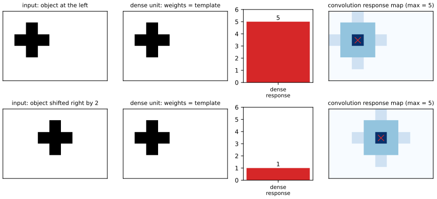
pp. 467–468 In Chapter 13 a hidden unit computes \(z_j=\varphi(\bm w_j^\T\bm x)\): it compares the input with a template \(\bm w_j\) and fires when they match. For an image \(\bm x\in\R^{W H C}\) this has three defects. (i) The weight matrix has a fixed shape, so a different size of image needs a different network. (ii) It is huge: a \(224\times224\) RGB image has \(150{,}528\) inputs, so one layer of 1000 hidden units has \(150{,}528{,}000\) weights, whereas 64 convolutional filters of size \(3\times3\times3\) have \(64\cdot27+64=1{,}792\) parameters. (iii) A template learned at one position is useless at another: the layer is not translation invariant, because the weights at different positions are unrelated (Figure 14.1). A convolutional neural network (CNN) replaces matrix multiplication by convolution with small filters, so the same template is compared with every patch (Figure 14.2, a photograph in the book).
14.2 Common layers
14.2.1 Convolutional layers
14.2.1.1 Convolution in 1d
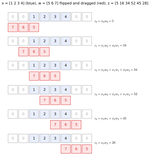
pp. 468–469 The convolution of two functions \(f,g:\R^D\to\R\) is \[ [f\circledast g](\bm z)=\int_{\R^D}f(\bm u)\,g(\bm z-\bm u)\,\d\bm u. \tag{14.1} \] For finite vectors, let \(\bm w\) hold the values \(f(-L),\dots,f(L)\) and \(\bm x\) the values \(g(-N),\dots,g(N)\); then \[ [\bm w\circledast\bm x](i)=w_{-L}x_{i+L}+\cdots+w_0x_i+\cdots+w_Lx_{i-L}, \tag{14.2} \] which is "flip \(\bm w\), drag it over \(\bm x\), multiply and add" (Figure 14.3). Without the flip one gets the cross-correlation \[ [\bm w\ast\bm x](i)=\sum_{u=-L}^{L}w_ux_{i+u},\qquad\text{or on the index set }\{0,\dots,L-1\}:\quad[\bm w\circledast\bm x](i)=\sum_{u=0}^{L-1}w_ux_{i+u}. \tag{14.3, 14.4} \] Deep-learning libraries, and this chapter, call the second operation "convolution". Since the filter is learned, the distinction is immaterial: a filter learned as a cross-correlation kernel is the flipped filter of the corresponding convolution.
Filling the gap 14.1: convolution and cross-correlation, the full output length, commutativity, and the polynomial picture pp. 468–469, (14.1)–(14.4)
Derivation
Discrete convolution. For finite sequences \(\bm x=(x_0,\dots,x_{m-1})\) and \(\bm w=(w_0,\dots,w_{l-1})\) extended by zero, define \(z_i=\sum_jw_jx_{i-j}\). The sum is non-zero only if \(0\le j\le l-1\) and \(0\le i-j\le m-1\), so \(z_i\ne0\) is possible only for \(0\le i\le m+l-2\): the full convolution has \(m+l-1\) entries, and the "valid" part (where the flipped filter lies inside the signal, \(l-1\le i\le m-1\)) has \(m-l+1\) entries. For Figure 14.3, \(m=4,l=3\): \(6\) full and \(2\) valid entries; e.g. \(z_2=x_2w_0+x_1w_1+x_0w_2=3\cdot5+2\cdot6+1\cdot7=34\).
Cross-correlation is convolution with the flipped filter. With \(\tilde w_j=w_{l-1-j}\), \((\bm w\ast\bm x)_i=\sum_{u=0}^{l-1}w_ux_{i+u}=\sum_{j}\tilde w_{j}x_{i+l-1-j}=(\tilde{\bm w}\circledast\bm x)_{i+l-1}\). So the two operations differ by a flip of the filter and a shift of the output index; if \(\bm w\) is symmetric (\(\tilde{\bm w}=\bm w\)) they coincide up to the shift, which is what the book says.
Commutativity. Substituting \(j'=i-j\), \(\sum_jw_jx_{i-j}=\sum_{j'}x_{j'}w_{i-j'}\): the full convolution is commutative, \(\bm w\circledast\bm x=\bm x\circledast\bm w\), and associative (the next paragraph). Cross-correlation is not commutative.
Polynomial picture. Attach to a sequence the polynomial \(P_{\bm x}(t)=\sum_ix_it^i\). Then \(P_{\bm w}(t)P_{\bm x}(t)=\sum_{j,i}w_jx_it^{i+j}=\sum_k\big(\sum_jw_jx_{k-j}\big)t^k=P_{\bm z}(t)\): the full convolution is polynomial multiplication, which makes commutativity and associativity obvious and gives the length \(m+l-1=\deg+1\). For Figure 14.3, \((1+2t+3t^2+4t^3)(5+6t+7t^2)=5+16t+34t^2+52t^3+45t^4+28t^5\) (confirmed numerically at random \(t\)). It also explains why stacking two convolutional layers with kernel size \(k\) gives an effective filter of size \(2k-1\) (before the nonlinearity): the polynomials multiply.
Continuous version. (14.1) is the same statement with sums replaced by integrals; \(\int f(\bm u)g(\bm z-\bm u)\d\bm u=\int g(\bm u)f(\bm z-\bm u)\d\bm u\) by the change of variable \(\bm u\to\bm z-\bm u\), and \(\widehat{f\circledast g}=\hat f\hat g\) for the Fourier transform (used for deconvolution in Section 14.4.2). \(\square\)
14.2.1.2 Convolution in 2d
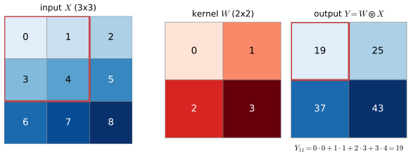
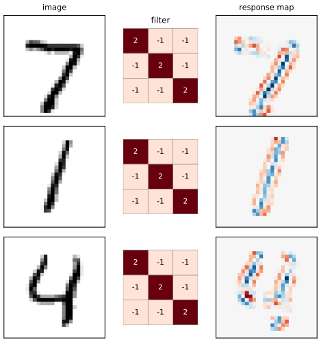
pp. 470–471 For an \(H\times W\) filter \(\bm W\), \[ [\bm W\circledast\bm X](i,j)=\sum_{u=0}^{H-1}\sum_{v=0}^{W-1}w_{u,v}\,x_{i+u,\,j+v}. \tag{14.5} \] For a \(3\times3\) input and a \(2\times2\) kernel \(\bm W=\begin{pmatrix}w_1&w_2\\w_3&w_4\end{pmatrix}\) the output is \(2\times2\) with entries \(w_1x_1+w_2x_2+w_3x_4+w_4x_5\), \(w_1x_2+w_2x_3+w_3x_5+w_4x_6\), \(w_1x_4+w_2x_5+w_3x_7+w_4x_8\), \(w_1x_5+w_2x_6+w_3x_8+w_4x_9\) (14.6, 14.7; Figure 14.5). The output at \((i,j)\) is large when the patch of \(\bm X\) at that position resembles \(\bm W\): template matching, so \(\bm Y=\bm W\circledast\bm X\) is a feature map (Figure 14.6: a diagonal-line template lights up on the diagonal strokes of a digit).
14.2.1.3 Convolution as matrix-vector multiplication
p. 471 Convolution is linear in \(\bm X\), so \(\vecop(\bm Y)=\bm C\,\vecop(\bm X)\) for a matrix \(\bm C\) built from the kernel; for (14.7) it is the \(4\times9\) matrix of (14.8)–(14.9) whose rows are shifted copies of \((w_1,w_2,0,w_3,w_4,0,0,0,0)\). A CNN layer is therefore an MLP layer whose weight matrix is sparse (a row has only \(k^2\) non-zeros) and tied (every row uses the same \(k^2\) numbers). This is the formal content of "translation invariance and far fewer parameters".
Filling the gap 14.2: the matrix of a convolution, parameter sharing, and translation equivariance p. 471, (14.8)–(14.9), p. 468
Derivation
The matrix. Number the input pixels row by row, \(\iota(a,b)=aW_{\rm in}+b\), and the outputs \(\omega(i,j)=iW_{\rm out}+j\). By (14.5) (with stride \(s\), padding \(p\), dilation \(r\), see Gap 14.3), \(y_{ij}=\sum_{u,v}w_{uv}\tilde x_{si+ru,\,sj+rv}\) where \(\tilde{\bm X}\) is \(\bm X\) padded with zeros. Hence
\[ C_{\omega(i,j),\,\iota(a,b)}=\sum_{u,v}w_{uv}\,\ind\{si+ru-p=a,\ sj+rv-p=b\}. \]
Each \((u,v)\) contributes to at most one column per row, so a row has at most \(k^2\) non-zeros; padding taps (\(a\) or \(b\) outside the image) are dropped, so border rows have fewer. The matrix is built in the code (conv_matrix); \(\bm C\,\vecop(\bm X)\) equals the direct computation for random sizes, strides, paddings and dilations. For the example of (14.8) (\(3\times3\), \(2\times2\), \(s=1\), \(p=0\)) rows 1 to 4 have their non-zero blocks at columns \((1,2,4,5)\), \((2,3,5,6)\), \((4,5,7,8)\), \((5,6,8,9)\).
Parameter counts. A dense layer between \(n_{\rm in}\) and \(n_{\rm out}\) units has \(n_{\rm in}n_{\rm out}\) weights; the convolution has \(k^2\) (per channel pair), whatever the image size: for a \(28\times28\) input and \(k=5\), \(p=2\) (so \(n_{\rm in}=n_{\rm out}=784\)) that is \(25\) against \(614{,}656\).
Translation equivariance. Let \(S_{\bm\tau}\) shift an image by \(\bm\tau\) with wrap-around (circular boundary), \((S_{\bm\tau}\bm X)_{ab}=x_{a-\tau_1,\,b-\tau_2}\), and let \(\bm Y=\bm W\circledast\bm X\) be the circular cross-correlation \(y_{ij}=\sum_{uv}w_{uv}x_{i+u,j+v}\). Then \[ (\bm W\circledast S_{\bm\tau}\bm X)_{ij}=\sum_{uv}w_{uv}x_{i+u-\tau_1,\,j+v-\tau_2}=y_{i-\tau_1,\,j-\tau_2}=(S_{\bm\tau}\bm Y)_{ij}, \] so \(\bm W\circledast S_{\bm\tau}=S_{\bm\tau}(\bm W\circledast\cdot)\): shifting the input shifts the feature map. This is equivariance (Section 14.2.2); it is exactly the statement that the matrix \(\bm C\) (here a doubly circulant matrix) commutes with the permutation matrices of the shifts. With zero padding the statement holds away from the border. The converse is also true: a linear map that commutes with all circular shifts is a circular convolution, because it is determined by the image of one basis vector \(\bm e_{0}\) and \(\bm e_{\bm\tau}=S_{\bm\tau}\bm e_0\).
Spectrum. A doubly circulant matrix is diagonalised by the 2-d discrete Fourier transform, so the singular values of the circular convolution layer are \(|\hat w(\bm\omega)|\), the magnitudes of the DFT of the zero-padded kernel; the layer is invertible iff \(\hat w\) has no zeros. This is why blurring (a kernel whose DFT is tiny at high frequencies) is hard to undo (Gap 14.12). \(\square\)
See also: Foundations of Deep Learning, 10.2.2 translation equivariance; Bayesian and Probabilistic ML, 5.5.6 convolutional networks; Introduction to Statistical Learning, 10.3.1 convolution layers.
14.2.1.4 Boundary conditions and padding
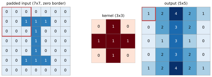
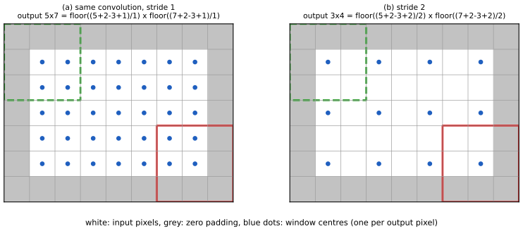
pp. 471–472 Convolving an \(f_h\times f_w\) filter with an \(x_h\times x_w\) image, using only positions where the filter lies inside the image ("valid" convolution), gives an output of size \((x_h-f_h+1)\times(x_w-f_w+1)\). To keep the size, pad the image with zeros (Figure 14.7); with \(p_h,p_w\) rows and columns of zeros on each side the output is \[ (x_h+2p_h-f_h+1)\times(x_w+2p_w-f_w+1), \tag{14.10} \] and with \(2p=f-1\) (odd \(f\)) the output has the size of the input ("same" convolution). For the \(5\times7\) input of Figure 14.8a with \(p=1\) and \(f=3\) the output is \((5+2-3+1)\times(7+2-3+1)=5\times7\) (14.11).
14.2.1.5 Strided convolution
p. 473 Neighbouring outputs of a convolution see overlapping inputs and are very similar. Evaluating the filter only at every \(s\)-th position (stride \(s\)) removes this redundancy and speeds up the computation. With padding \(p\) and stride \(s\) the output size is \[ \Big\lfloor\frac{x_h+2p_h-f_h+s_h}{s_h}\Big\rfloor\times\Big\lfloor\frac{x_w+2p_w-f_w+s_w}{s_w}\Big\rfloor. \tag{14.12} \] For Figure 14.8b (\(5\times7\), \(f=3\), \(p=1\), \(s=2\)): \(\lfloor(5+2-3+2)/2\rfloor\times\lfloor(7+2-3+2)/2\rfloor=3\times4\) (14.13).
Filling the gap 14.3: the output-size formulas (14.10)–(14.13), same convolution, and dilation pp. 471–473
Derivation
Counting windows. Take one dimension: input length \(n\), padded length \(n+2p\), filter taps at offsets \(0,r,2r,\dots,r(k-1)\) (\(r=1\) is an ordinary filter; \(r\) is the dilation of Section 14.4.1). The window of output \(i\) starts at padded position \(si\) and reads positions \(si,si+r,\dots,si+r(k-1)\). It fits iff \(si+r(k-1)\le n+2p-1\), i.e. \(i\le\frac{n+2p-1-r(k-1)}{s}\). The outputs are \(i=0,1,\dots,\lfloor\frac{n+2p-1-r(k-1)}{s}\rfloor\), so \[ n_{\rm out}=\Big\lfloor\frac{n+2p-r(k-1)-1}{s}\Big\rfloor+1. \] For \(r=1\), \(s=1\) this is \(n+2p-k+1\), which is (14.10). For \(r=1\) and general \(s\), \(\lfloor\frac{n+2p-k}{s}\rfloor+1=\lfloor\frac{n+2p-k+s}{s}\rfloor\), which is (14.12) (the identity \(\lfloor a/s\rfloor+1=\lfloor(a+s)/s\rfloor\) holds for every integer \(a\)). A direct enumeration over all \(n\in[5,19]\), \(k\le5\), \(p\le2\), \(s\le3\) confirms it.
Same convolution. \(n_{\rm out}=n\) for \(s=r=1\) iff \(2p=k-1\); this needs \(k\) odd. For even \(k\) one pads \(\lfloor(k-1)/2\rfloor\) on one side and \(\lceil(k-1)/2\rceil\) on the other (asymmetric padding), the reason odd filter sizes are standard. With stride \(s\) and total padding \(2p\) one gets \(\lceil n/s\rceil\) when \(2p\) is chosen as the smallest value with \(n_{\rm out}\ge\lceil n/s\rceil\).
Examples. (14.11): \((5+2-3+1,\,7+2-3+1)=(5,7)\). (14.13): rows \(\lfloor6/2\rfloor=3\), columns \(\lfloor8/2\rfloor=4\) (the book prints the column term as \(\lfloor4/1\rfloor\); the value 4 is right, but the numerator is \(7+2-3+2=8\) and the denominator 2, see the notes on the book).
A stack of layers. The size is computed layer by layer; for the LeNet5 of Figure 14.16a, input \(28\), \(5\times5\) conv with \(p=2\): \(28\); pool \(2\), stride 2: \(14\); \(5\times5\) conv, \(p=0\): \(10\); pool: \(5\); so the dense layer sees \(16\cdot5\cdot5=400\) inputs. \(\square\)
14.2.1.6 Multiple input and output channels
pp. 473–474 An image has \(C\) channels (RGB, hyperspectral bands). A kernel for it is a 3-d array \(\bm W\in\R^{H\times W\times C}\): convolve channel \(c\) with \(\bm W_{:,:,c}\) and sum over channels, adding a bias \(b\) and with stride \(s\), \[ z_{i,j}=b+\sum_{u=0}^{H-1}\sum_{v=0}^{W-1}\sum_{c=0}^{C-1}x_{si+u,\,sj+v,\,c}\,w_{u,v,c}. \tag{14.14} \] To detect \(D\) kinds of features the filter becomes a 4-d array \(\bm W_{:,:,c,d}\) and \[ z_{i,j,d}=b_d+\sum_{u=0}^{H-1}\sum_{v=0}^{W-1}\sum_{c=0}^{C-1}x_{si+u,\,sj+v,\,c}\,w_{u,v,c,d}. \tag{14.15} \] The vector \(z_{i,j,1:D}\) at one location is the hypercolumn (Figure 14.10, a diagram). A layer with \(C\) input and \(D\) output channels and \(k\times k\) filters has \(k^2CD+D\) parameters.

14.2.1.7 1 × 1 (pointwise) convolution
pp. 474–475 A \(1\times1\) convolution mixes channels at each location without looking at neighbours, \[ z_{i,j,d}=b_d+\sum_{c=0}^{C-1}x_{i,j,c}\,w_{0,0,c,d}, \tag{14.16} \] which changes the number of channels from \(C\) to \(D\) and is a one-layer MLP applied to every hypercolumn in parallel (Figure 14.11).

Filling the gap 14.4: multi-channel convolution as one matrix product, and 1 × 1 convolution pp. 473–475, (14.14)–(14.16)
Derivation
The im2col form. For one image, collect for every output position \((i,j)\) the patch \(\bm p_{ij}=(x_{si+u,sj+v,c})_{u,v,c}\in\R^{k^2C}\), and stack the filters as the rows of \(\bm W_{\rm mat}\in\R^{D\times k^2C}\) (row \(d\) is \(\bm W_{:,:,:,d}\) flattened in the same order). Then (14.15) says \(\bm z_{ij}=\bm W_{\rm mat}\bm p_{ij}+\bm b\): the whole layer is the single matrix product \[ \bm Z=\bm W_{\rm mat}\,\bm P+\bm b\bm 1^\T,\qquad\bm P=[\bm p_{ij}]\in\R^{k^2C\times H_{\rm out}W_{\rm out}}, \] which is how convolutions are computed on GPUs (a large GEMM). Counting: parameters \(k^2CD+D\); multiplications \(H_{\rm out}W_{\rm out}\cdot Dk^2C\). A batch of \(N\) images adds the factor \(N\). The matrix \(\bm C\) of Gap 14.2 for the multi-channel layer is the Kronecker-structured block matrix with blocks \(\bm C_{dc}\), the single-channel matrix for the kernel \(\bm W_{:,:,c,d}\).
1 × 1 convolution. For \(k=1\), \(s=1\), \(p=0\): \(\bm P\) is just the input reshaped to \(C\times HW\), and \(\bm Z=\bm W_{\rm mat}\bm P+\bm b\bm 1^\T\) with \(\bm W_{\rm mat}\in\R^{D\times C}\): a dense layer shared by all pixels. For Figure 14.11 numerically: \(\bm W_{\rm mat}=\begin{pmatrix}1&0&2\\0&1&-1\end{pmatrix}\) and the outputs equal \(\bm W_{\rm mat}\) times the column of channel values at every pixel (confirmed against a library convolution). It has \(CD+D\) parameters: reducing \(C=256\) channels to \(D=64\) costs \(16{,}448\) numbers and is the "bottleneck" of Inception and ResNet (Gap 14.9).
Layouts. The book stores a filter as \((H,W,C,D)\) and a batch as \((N,H,W,C)\) (NHWC, TensorFlow). PyTorch uses \((D,C,H,W)\) and \((N,C,H,W)\). The notes and the code use the second layout; the formulas above are layout-independent. \(\square\)
14.2.2 Pooling layers
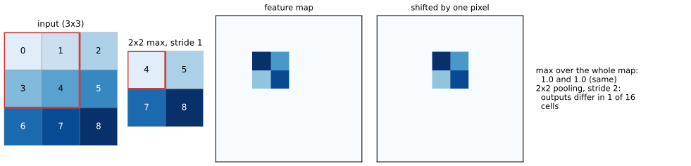
pp. 475–476 Convolution is equivariant to translations: it preserves where a feature is, up to the resolution. For classification we usually want invariance: whether a face is present, not where. Max pooling replaces each window by its maximum (Figure 14.12), average pooling by the mean; pooling is applied to each channel separately. Global average pooling averages a whole \(H\times W\times D\) map down to a \(D\)-vector, which can be fed to a dense layer and a softmax; because the vector has the same length for any image size, the classifier works on images of any size.
Filling the gap 14.5: equivariance, invariance and what pooling achieves; backpropagation through max pooling pp. 475–476
Derivation
Definitions. A map \(f\) is equivariant to a group of transformations \(\{T_g\}\) if \(f(T_g\bm x)=T'_gf(\bm x)\) for all \(g\) (for convolution \(T'_g=T_g\), the same shift, Gap 14.2), and invariant if \(f(T_g\bm x)=f(\bm x)\).
Global pooling is invariant to circular shifts. Let \(S_{\bm\tau}\) be a circular shift. Then \(\sum_{a,b}x_{a-\tau_1,b-\tau_2}=\sum_{a,b}x_{a,b}\) (a re-indexing of the same sum, valid because the shift is a bijection of the grid) and \(\max_{a,b}x_{a-\tau_1,b-\tau_2}=\max_{a,b}x_{a,b}\); so global average and global max pooling are invariant. Composing with an equivariant convolution gives an invariant feature \(g(\bm X)=\operatorname{pool}(\bm W\circledast\bm X)\), the reason a conv-pool network detects "a cross is somewhere in the image" (Figure 14.1). With zero padding and finite images the statement holds as long as the object does not leave the image.
Local pooling is only approximately invariant. For \(P\times P\) pooling with stride \(P\), shifting the input by a multiple of \(P\) shifts the output exactly (equivariance with stride \(P\)), but a shift by one pixel can change several outputs: in Figure 14.12 one of 16 changes. The invariance is therefore approximate and local, and grows with the depth of pooling layers (the receptive field of a unit increases, Gap 14.6).
Gradient of max pooling. \(y=\max_{k\in\text{window}}x_k\) is piecewise linear in \(\bm x\) with \(\partial y/\partial x_k=\ind\{k=\arg\max\}\) wherever the maximiser is unique (at ties \(y\) is not differentiable and one picks any maximiser; the set of ties has measure zero for continuous data). So backpropagation routes the incoming gradient to the arg-max pixel and sends zero to the others; for average pooling the gradient is spread equally, \(1/P^2\) per input. Both are implemented in the code and match automatic differentiation (cnn_backward). \(\square\)
14.2.3 Putting it all together
p. 476 A typical CNN alternates convolution (plus nonlinearity) and pooling, then flattens or globally pools and applies a linear classifier (Figure 14.13, a diagram). The pattern goes back to Fukushima's neocognitron (1975), is motivated by Hubel and Wiesel's simple and complex cells (1962), and was trained by backpropagation and SGD in LeCun's LeNet (1998). Stacking layers enlarges the region of the input that one unit depends on, its receptive field.
Filling the gap 14.6: receptive fields of stacked convolutions, and why three 3 × 3 layers beat one 7 × 7 p. 481 (AlexNet paragraph), pp. 486–487
Derivation
Receptive-field recursion. Layer \(l\) has kernel size \(k_l\), stride \(s_l\) and dilation \(r_l\) (\(r_l=1\) for ordinary filters). Let \(R_l\) be the width of the set of input pixels that one unit of layer \(l\) depends on, and \(J_l=\prod_{m\le l}s_m\) the "jump", the spacing in input pixels of adjacent units of layer \(l\) (\(R_0=J_0=1\)). Claim: \[ R_l=R_{l-1}+r_l(k_l-1)J_{l-1},\qquad J_l=J_{l-1}s_l. \] Proof. A unit of layer \(l\) reads \(k_l\) units of layer \(l-1\) at spacing \(r_l\); those span \(r_l(k_l-1)+1\) consecutive-with-gaps positions of layer \(l-1\). Adjacent units of layer \(l-1\) are \(J_{l-1}\) input pixels apart, so the leftmost and rightmost of the \(k_l\) units are \(r_l(k_l-1)J_{l-1}\) input pixels apart; adding the receptive field \(R_{l-1}\) of one unit of layer \(l-1\) (which extends over the same width at the ends, overlapping) gives \(R_l=R_{l-1}+r_l(k_l-1)J_{l-1}\). The recursion for \(J\) is the definition. \(\square\)
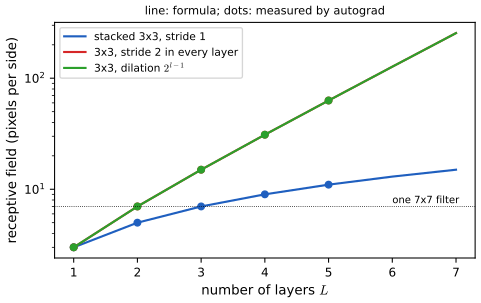
Consequences. (i) \(L\) layers with \(k=3\), \(s=1\), \(r=1\): \(R_L=1+2L\), so \(L=3\) gives 7, as the book says. (ii) The same with stride 2 in every layer: \(J_{l-1}=2^{l-1}\), \(R_L=1+2\sum_{l=1}^L2^{l-1}=2^{L+1}-1\): exponential. (iii) With dilations \(r_l=2^{l-1}\) and stride 1: \(R_L=1+2\sum_l2^{l-1}=2^{L+1}-1\) (Gap 14.11). The formulas agree with the support of the gradient of a unit with respect to the input, computed by automatic differentiation for several stacks (Figure 14.S3).
Parameters. With \(C\) channels in and out, three \(3\times3\) layers have \(3\cdot9C^2=27C^2\) weights and one \(7\times7\) layer has \(49C^2\); the stack has the same receptive field, 45% fewer weights, and two extra nonlinearities, so it can represent more functions, hence the preference in modern networks (the book's statement, Section 14.3.2). \(\square\)
14.2.4 Normalization layers
p. 476 Shallow CNNs train with plain conv-pool stacks; deeper ones suffer from vanishing or exploding gradients (Section 13.4.2). A common remedy is a layer that standardises the hidden activations to zero mean and unit variance, as one standardises the inputs (Section 10.2.8).
14.2.4.1 Batch normalization
pp. 477–478 Batch normalisation (Ioffe and Szegedy, 2015) replaces the activation vector \(\bm z_n\) of example \(n\) in a layer by \[ \tilde{\bm z}_n=\bm\gamma\odot\hat{\bm z}_n+\bm\beta,\qquad\hat{\bm z}_n=\frac{\bm z_n-\bm\mu_{\mathcal B}}{\sqrt{\bm\sigma^2_{\mathcal B}+\epsilon}}, \tag{14.17, 14.18} \] \[ \bm\mu_{\mathcal B}=\frac1{|\mathcal B|}\sum_{\bm z\in\mathcal B}\bm z,\qquad\bm\sigma^2_{\mathcal B}=\frac1{|\mathcal B|}\sum_{\bm z\in\mathcal B}(\bm z-\bm\mu_{\mathcal B})^2, \tag{14.19, 14.20} \] where \(\mathcal B\) is the minibatch containing \(n\), \(\bm\gamma,\bm\beta\) are learned and \(\epsilon>0\) is small. For a convolutional layer the average runs over the batch and over all spatial positions but not over channels (one \(\mu,\sigma\) per channel; footnote 3 of the book). The mean and variance of internal layers change as the parameters change, so they are recomputed on every minibatch. At test time, after training one freezes \(\bm\mu,\bm\sigma^2\) to their values on the training set (in practice an exponential moving average), so that a single example can be processed. A frozen batch-norm layer after a linear layer \(\bm X\bm W+\bm b\) can be merged into it ("fused batch norm"): \(\bm W'=\bm\gamma\odot\bm W/\bm\sigma\), \(\bm b'=\bm\gamma\odot(\bm b-\bm\mu)/\bm\sigma+\bm\beta\).
Filling the gap 14.7: the gradient of batch normalisation, scale invariance, the train/test mismatch and the fused layer pp. 477–478, (14.17)–(14.20)
Derivation
Backward pass. Fix one channel (scalar activations) and write \(m\) for the number of pooled values (\(m=NHW\) for a conv layer), \(\tilde\sigma=\sqrt{\sigma^2+\epsilon}\), \(\hat z_i=(z_i-\mu)/\tilde\sigma\). Then \(\partial\mu/\partial z_j=1/m\) and \(\partial\sigma^2/\partial z_j=2(z_j-\mu)/m\) (the terms from \(\partial\mu/\partial z_j\) vanish because \(\sum_i(z_i-\mu)=0\)), so \[ \frac{\partial\hat z_i}{\partial z_j}=\frac{1}{\tilde\sigma}\Big(\delta_{ij}-\frac1m\Big)-\frac{z_i-\mu}{2\tilde\sigma^3}\cdot\frac{2(z_j-\mu)}{m}=\frac1{\tilde\sigma}\Big(\delta_{ij}-\frac1m-\frac{\hat z_i\hat z_j}{m}\Big), \] using \(z_i-\mu=\tilde\sigma\hat z_i\) (so \((z_i-\mu)(z_j-\mu)/\tilde\sigma^2=\hat z_i\hat z_j\)). Let \(L\) depend on the outputs \(\tilde z_i=\gamma\hat z_i+\beta\) with upstream gradients \(g_i=\partial L/\partial\tilde z_i\) and put \(\hat g_i=\gamma g_i\). Then \[ \frac{\partial L}{\partial z_j}=\sum_i\hat g_i\frac{\partial\hat z_i}{\partial z_j}=\frac1{\tilde\sigma}\Big(\hat g_j-\overline{\hat g}-\hat z_j\,\overline{\hat g\hat z}\Big),\qquad\frac{\partial L}{\partial\gamma}=\sum_ig_i\hat z_i,\quad\frac{\partial L}{\partial\beta}=\sum_ig_i, \] with bars denoting averages over the \(m\) values. This agrees with automatic differentiation (checked on random tensors). Two consequences: the gradient with respect to the input sums to zero (\(\sum_j\partial L/\partial z_j=0\): adding a constant to all inputs of a channel changes nothing) and is orthogonal to \(\hat{\bm z}\) when \(\epsilon=0\) (\(\sum_j\hat z_j\partial L/\partial z_j=\tilde\sigma^{-1}\,m\,\overline{\hat g\hat z}\,(1-\overline{\hat z^2})=0\), because \(\overline{\hat z}=0\) and \(\overline{\hat z^2}=\sigma^2/\tilde\sigma^2=1\) when \(\epsilon=0\)): the layer removes the components of the gradient along the directions it normalises away.
Scale invariance. Let a unit be \(\bm w^\T\bm x\) followed by batch norm without \(\epsilon\). Then \(\operatorname{BN}(c\,\bm w^\T\bm x)=\operatorname{BN}(\bm w^\T\bm x)\) for every \(c>0\), because mean and standard deviation scale by \(c\). If the loss \(L(\bm w)\) depends on \(\bm w\) only through this unit, \(L(c\bm w)=L(\bm w)\); differentiating in \(c\) at \(c=1\) gives \(\bm w^\T\nabla L(\bm w)=0\), and differentiating \(L(c\bm w)=L(\bm w)\) in \(\bm w\) gives \(\nabla L(c\bm w)=\nabla L(\bm w)/c\). So (i) gradient steps are orthogonal to \(\bm w\), hence each step increases \(\|\bm w\|\): \(\|\bm w-\eta\nabla L\|^2=\|\bm w\|^2+\eta^2\|\nabla L\|^2\); (ii) the effective learning rate on the direction \(\bm w/\|\bm w\|\) is \(\eta/\|\bm w\|^2\). This is one reason for the reduced sensitivity to the learning rate that the book mentions, and why batch norm interacts with weight decay. (Confirmed numerically: \(\operatorname{BN}(3.7\,\bm W\bm x)=\operatorname{BN}(\bm W\bm x)\).)
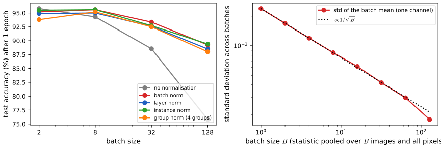
Train and test. In training mode \(\bm\mu_{\mathcal B},\bm\sigma^2_{\mathcal B}\) are random (depend on which examples are in the batch): for \(B\) independent examples with per-pixel variance \(v\) the batch mean has variance \(v/(B\cdot HW)\) if all \(BHW\) values were independent, and in general decreases with \(B\); in Figure 14.S2 the standard deviation of the batch mean of a first-layer channel falls close to \(B^{-1/2}\) (a factor 13.5 from \(B=1\) to 128, against 11.3), the difference coming from the correlation of neighbouring pixels and of images. This noise acts as a regulariser and is why small batches hurt: with \(B=1\) in training mode the layer becomes instance normalisation. At test time the frozen \(\bm\mu,\bm\sigma^2\) make the layer an affine map \(z\mapsto\gamma(z-\mu)/\tilde\sigma+\beta\), deterministic per example, which is the reason for the train/test difference of Section 14.2.4.1.
Fused batch norm. For \(\bm a=\bm W\bm x+\bm b\) (one row \(\bm w_j\) per output unit) the frozen layer gives \(\gamma_j(a_j-\mu_j)/\sigma_j+\beta_j=(\gamma_j/\sigma_j)\bm w_j^\T\bm x+\gamma_j(b_j-\mu_j)/\sigma_j+\beta_j\), i.e. \(\bm w_j'=(\gamma_j/\sigma_j)\bm w_j\) and \(b_j'=\gamma_j(b_j-\mu_j)/\sigma_j+\beta_j\), which are the book's \(\bm W'=\bm\gamma\odot\bm W/\bm\sigma\) and \(\bm b'\) (with \(\bm\sigma\) including \(\epsilon\) and the row convention). For a convolution the same holds per output channel because the layer is linear in the filter. \(\square\)
Not proved here. That batch norm "makes the optimisation landscape smoother" (Santurkar et al., 2018) and "is a form of approximate Bayesian inference" (Teye et al., 2018; Luo et al., 2019) are results of the cited papers; the notes use only the exact statements above.
See also: Foundations of Deep Learning, 7.4.2 batch normalization and 7.4.3 layer normalization.
14.2.4.2 Other kinds of normalization layer
pp. 478–479 Batch norm needs a decent batch. The remedy is to pool statistics over other axes. Index an activation by \(i=(i_N,i_H,i_W,i_C)\) and let \(S_i\) be the set over which to average: \[ \mu_i=\frac1{|S_i|}\sum_{k\in S_i}z_k,\qquad\sigma_i=\sqrt{\frac1{|S_i|}\sum_{k\in S_i}(z_k-\mu_i)^2+\epsilon},\qquad\tilde z_i=\gamma_c\frac{z_i-\mu_i}{\sigma_i}+\beta_c. \tag{14.21} \] Batch norm takes \(S_i\) = all positions (batch, height, width) with the same channel as \(i\); layer norm (Ba et al., 2016) all channels, heights and widths of the same example; instance norm (Ulyanov et al., 2016) the heights and widths of the same example and channel; group norm (Wu and He, 2018) the same example and a group of channels (Figure 14.14). Layer norm is group norm with one group, instance norm is group norm with \(C\) groups. Filter response normalisation (Singh and Krishnan, 2020) divides by the root mean square \(\nu^2=\frac1{HW}\sum z^2\) of each (example, channel) map without subtracting the mean, followed by a thresholded linear unit \(\max(x,\tau)\).

Filling the gap 14.8: the normalisation family as pooling sets, special cases, and filter response normalisation pp. 478–479, (14.21)
Derivation
Sizes of the sets. For a tensor with \(N\) examples, \(C\) channels and \(H\times W\) pixels: batch norm \(|S_i|=NHW\); layer norm \(|S_i|=CHW\); instance norm \(|S_i|=HW\); group norm with \(G\) groups \(|S_i|=(C/G)HW\) (\(G\) divides \(C\)). Group norm interpolates: \(G=1\) is layer norm, \(G=C\) is instance norm, by comparing the index sets. In Figure 14.14 (\(N=4,C=6\)) the sets have \(4,6,1,3\) blocks.
What each guarantees. By construction, over every pooling set \(S\) the normalised values \(\hat z_k=(z_k-\mu)/\sigma\) have mean exactly 0 and variance \(\sigma_0^2/(\sigma_0^2+\epsilon)\) (\(\sigma_0^2\) the biased sample variance), i.e. unit variance up to \(\epsilon\): \(\frac1{|S|}\sum(\hat z_k)^2=\sigma_0^2/(\sigma_0^2+\epsilon)\). Batch norm shares one \((\mu,\sigma)\) between all examples of the batch, so it preserves differences between examples (their relative offsets and gains) and couples them; layer, instance and group norm are computed per example, are independent of the batch size and behave identically in training and testing. Instance norm in addition removes each example's per-channel offset and gain; that is why it suits style-transfer networks (contrast and mean colour belong to the style, Section 14.6.5).
Why the choice matters. If channels have very different scales (channel means \(0,2,-1,4,\dots\) in the demonstration), layer norm uses one scale for all and lets the large channels dominate; batch and instance norm treat each channel separately. Statistics estimated from fewer values are noisier: the standard deviation of the mean of \(|S|\) approximately independent values scales like \(|S|^{-1/2}\), so instance norm (\(|S|=HW\)) is the noisiest per example and batch norm with a tiny batch inherits the same noise.
Filter response normalisation. For one (example, channel) map \(\bm z\in\R^{HW}\) put \(\nu^2=\frac1{HW}\sum z_k^2\) and \(\hat z_k=z_k/\sqrt{\nu^2+\epsilon}\). Then \(\frac1{HW}\sum\hat z_k^2=\nu^2/(\nu^2+\epsilon)\approx1\): unit mean square but, as there is no centring, any mean of the map survives (it is scaled by \(1/\nu\)) and activations can drift away from zero. The authors compensate with the threshold \(\tau\) in \(\max(x,\tau)\), a ReLU with a learned offset. It uses no batch statistics, so it works for \(B=1\).
Normalizer-free networks (Brock et al., 2021) drop normalisation and use adaptive gradient clipping (13.70) with a clipping strength set per layer from the ratio of gradient to weight norm; this is a method description in the book and nothing further is proved here. \(\square\)
14.2.4.3 Normalizer-free networks
p. 479 Brock et al. (2021) train deep residual networks without any normalisation layer: instability is controlled instead by adaptive gradient clipping, a variant of (13.70) whose clipping threshold adapts to the size of each weight matrix. The resulting models train faster and reach higher accuracy than comparable batch-norm networks, according to the paper (not reproduced here).
14.3 Common architectures for image classification
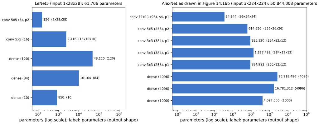
p. 479 Image classification estimates \(f:\R^{H\times W\times K}\to\{0,1\}^C\) (\(K\) input channels, \(C\) classes). This section reviews the networks that shaped the field. Figure 14.16 below gives, for LeNet5 and for AlexNet as the book draws it, the output shape and the number of parameters of every layer, computed with the formulas of the previous section; the diagrams of Figures 14.15, 14.19, 14.20, 14.21 and 14.22 carry the same information.
14.3.1 LeNet
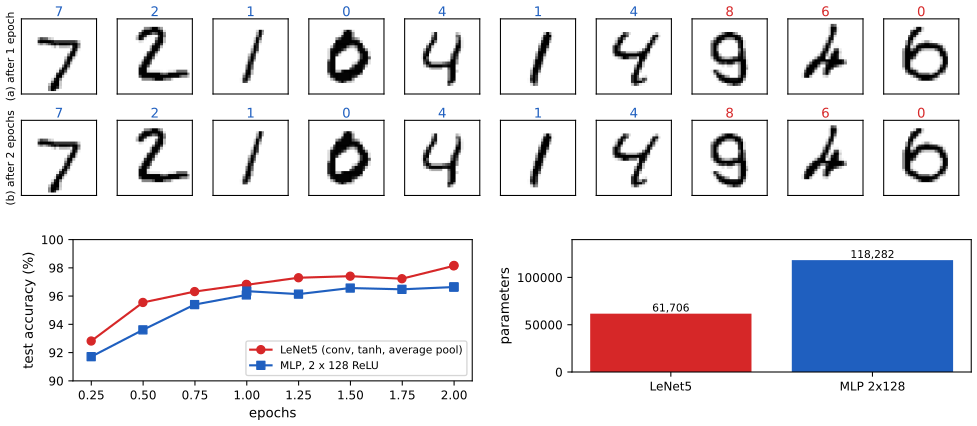
pp. 479–481 LeNet5 (LeCun et al., 1998) classifies \(28\times28\) digits: \(5\times5\) convolution with 6 channels and padding 2, \(2\times2\) average pooling, \(5\times5\) convolution with 16 channels, pooling, and dense layers of 120, 84 and 10 units (Figures 14.15 and 14.16a). The book reports a test accuracy of 98.8% after one epoch, against 95.9% for the MLP of Section 13.2.4.2, and Figure 14.17 shows predictions on cherry-picked digits including errors. LeNet was combined with a model like a conditional random field to read strings of digits and was deployed by the US postal service.
14.3.2 AlexNet
pp. 481–482 AlexNet (Krizhevsky et al., 2012) lowered the top-5 error on ImageNet from 26% to 15%. It resembles LeNet but is deeper (8 weight layers, 5 convolutional and 3 dense), uses ReLU instead of tanh, uses dropout instead of weight decay, and stacks several convolutional layers instead of alternating strictly with pooling. Stacked layers enlarge the receptive field while keeping fewer parameters than one large filter: three \(3\times3\) filters see \(7\times7\) pixels with \(27C^2\) instead of \(49C^2\) weights (Gap 14.6). It has about 60 million parameters, mostly in the dense layers, for 1.2 million training images (Gap 14.9).
14.3.3 GoogLeNet (Inception)
p. 482 GoogLeNet (Szegedy et al., 2015) is built from inception blocks with parallel branches of different filter sizes (\(1\times1\), \(3\times3\), \(5\times5\) and pooling) whose outputs are concatenated along the channel axis, so that the network learns which filter size to use at each level; \(1\times1\) convolutions first reduce the number of channels to cut the cost (Figures 14.18 and 14.19). The full model stacks nine inception blocks followed by global average pooling. The saving from the \(1\times1\) reduction is computed in Gap 14.9.
Filling the gap 14.9: exact parameter counts, the Inception bottleneck, and the down-sampling factor of ResNet-18 pp. 479–484, Figures 14.15–14.21
Derivation
LeNet5. A convolution with \(C\) input and \(D\) output channels and a \(k\times k\) filter has \(k^2CD+D\) parameters, a dense layer \(n_{\rm in}n_{\rm out}+n_{\rm out}\). Layers: conv \(1\to6\), \(5\times5\): \(150+6=156\); conv \(6\to16\), \(5\times5\): \(2400+16=2{,}416\); dense \(400\to120\): \(48{,}000+120=48{,}120\); dense \(120\to84\): \(10{,}164\); dense \(84\to10\): \(850\). Total \(61{,}706\) (confirmed by a library count). The shapes follow (14.10), (14.12): \(28\to28\) (\(p=2\)) \(\to14\) (pool) \(\to10\) \(\to5\), so the flattened size is \(16\cdot25=400\).
AlexNet (Figure 14.16b of the book). Input \(3\times224\times224\). conv \(11\times11\), 96, stride 4, padding 1: \(\lfloor(224+2-11+4)/4\rfloor=54\), parameters \(34{,}944\); max pool \(3\), stride 2: \(26\); conv \(5\times5\), 256, padding 2: \(614{,}656\) parameters, size 26; pool: 12; three \(3\times3\) convs with 384, 384, 256 channels: \(885{,}120+1{,}327{,}488+884{,}992\); pool: \(5\); flatten \(256\cdot25=6400\); dense \(6400\to4096\): \(26{,}218{,}496\); \(4096\to4096\): \(16{,}781{,}312\); \(4096\to1000\): \(4{,}097{,}000\). Total \(50{,}844{,}008\) (library count agrees), of which \(47{,}096{,}808\) (92.6%) are in the dense layers. For the original network, whose last pooling gives \(6\times6\times256=9216\) inputs, the three dense layers alone have \(9216\cdot4096+4096+16{,}781{,}312+4{,}097{,}000=58.6\) million and the convolutions add about 2 to 4 million (the original splits channels over two GPUs), which is the book's "60 million"; "mostly due to the three fully connected layers" holds in both versions.
Inception bottleneck (illustrative numbers). Take 192 input channels and a branch that must output 128 channels with a \(3\times3\) filter. Directly: \(9\cdot192\cdot128=221{,}184\) weights. With a \(1\times1\) reduction to 96 channels first: \(192\cdot96+9\cdot96\cdot128=18{,}432+110{,}592=129{,}024\) weights, 42% fewer, and the same factor in multiplications at fixed image size. The \(1\times1\) layer changes the number of channels without touching the spatial size (Gap 14.4); the price is one more nonlinearity and a rank constraint on the composed filter.
ResNet-18. A \(3\times3\) conv-BN with \(c_{\rm in},c_{\rm out}\) channels (no conv bias) has \(9c_{\rm in}c_{\rm out}+2c_{\rm out}\) parameters; a \(1\times1\) projection \(c_{\rm in}c_{\rm out}+2c_{\rm out}\). Stem: \(7\times7\), \(3\to64\): \(9{,}408+128\). Stages with \(64,128,256,512\) channels, two basic blocks each (two \(3\times3\) convs), the first block of stages 2 to 4 having stride 2 and a \(1\times1\) projection. Fully connected \(512\to1000\): \(513{,}000\). Total \(11{,}689{,}512\) (library count agrees). Weight layers: stem 1 + 8 blocks \(\times\) 2 + dense 1 = 18 (the \(1\times1\) projections are not counted in the name). Down-sampling: the stem convolution (stride 2), the max pool (stride 2), and three stride-2 stages: \(2^5=32\), so \(224\to112\to56\to28\to14\to7\), as the book says.
Why the dense layers dominate. A dense layer after a feature map of \(H'W'D\) numbers has \(H'W'D\cdot n_{\rm out}\) weights, while a convolution has \(k^2CD\), independent of the image size. This is the reason later architectures end with global average pooling (a \(D\)-vector) instead of flattening. \(\square\)
14.3.4 ResNet
pp. 483–484 The winner of ImageNet 2015 (He et al., 2016a) replaced \(\bm x_{l+1}=\mathcal F_l(\bm x_l)\) by the residual block \[ \bm x_{l+1}=\varphi\big(\bm x_l+\mathcal F_l(\bm x_l)\big), \tag{14.22} \] so that \(\mathcal F_l\) (conv-BN-ReLU-conv-BN) only learns the difference between input and output; a \(1\times1\) convolution on the skip path matches channel counts when they change (Figure 14.20). Gradients flow directly through the skip connections, which allows hundreds of layers (152 in the paper; the book's Figure 14.21 shows ResNet-18). He et al. (2016b) showed that the signal on the skip path is still attenuated by the nonlinearity after the addition and proposed the pre-activation block \[ \bm x_{l+1}=\bm x_l+\varphi\big(\mathcal F_l(\bm x_l)\big), \tag{14.23} \] in which the identity is exact (use \(\mathcal F_l=\bm 0\)); it trains networks with 1001 layers. A wide ResNet (Zagoruyko and Komodakis, 2016) uses many channels instead of great depth.
Filling the gap 14.10: gradient flow in a residual network (the \(2^L\) paths) and DenseNet growth pp. 483–485, (14.22)–(14.24); Section 13.4.4
Derivation
Pure identity skips. Let \(\bm x_{i+1}=\bm x_i+\mathcal F_i(\bm x_i)\) for \(i=l,\dots,L-1\) with Jacobians \(\bm J_i=\partial\mathcal F_i/\partial\bm x_i\). Unrolling, \(\bm x_L=\bm x_l+\sum_{i=l}^{L-1}\mathcal F_i(\bm x_i)\). By the chain rule \(\partial\bm x_L/\partial\bm x_l=(\bm I+\bm J_{L-1})\cdots(\bm I+\bm J_l)\). Expanding the product, \[ \prod_{i}(\bm I+\bm J_i)=\sum_{S\subseteq\{l,\dots,L-1\}}\ \prod_{i\in S}^{\rightarrow}\bm J_i, \] a sum over the \(2^{L-l}\) subsets of blocks that a signal may pass through (each block is either skipped, factor \(\bm I\), or entered, factor \(\bm J_i\)); I checked the identity numerically for \(L-l=4\) random matrices. The term \(S=\emptyset\) is \(\bm I\): the gradient of the loss at \(\bm x_L\) reaches \(\bm x_l\) unchanged, whatever the other blocks do, so \(\partial L/\partial\bm x_l=\partial L/\partial\bm x_L\,(\bm I+\text{terms})\) cannot vanish because the product of Jacobians does. In a plain network the only term is \(\prod\bm J_i\), a product of \(L-l\) matrices whose norm typically decays or explodes geometrically (Section 13.4.2). The expansion also shows the other side: if the \(\bm J_i\) have norms \(\ge\rho\), the gradient can grow like \((1+\rho)^{L-l}\), which is why residual networks are combined with normalisation and careful initialisation.
Post-activation block (14.22). With \(\bm x_{i+1}=\varphi(\bm x_i+\mathcal F_i(\bm x_i))\) the Jacobian is \(\bm D_i(\bm I+\bm J_i)\) with \(\bm D_i=\diag\varphi'\), which for ReLU is a 0/1 mask. The product \(\prod_i\bm D_i(\bm I+\bm J_i)\) contains the masks on the identity path too; every zeroed unit cuts the skip path, which is the attenuation observed by He et al. (2016b). In the pre-activation form (14.23) the identity path has no nonlinearity, \(\bm x_{l+1}=\bm x_l+\varphi(\mathcal F_l(\bm x_l))\), so the term \(S=\emptyset\) stays exactly \(\bm I\). Ease of learning the identity: with \(\mathcal F_l\) whose last layer has zero weights, \(\bm x_{l+1}=\bm x_l\) exactly in (14.23); in (14.22) it equals \(\varphi(\bm x_l)=\bm x_l\) only if \(\bm x_l\ge0\), which is the case when \(\bm x_l\) is itself the output of a ReLU.
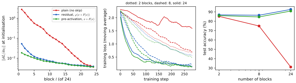
What the experiment shows. For networks of 2, 8 and 24 blocks (two convolutions and batch norm each, width 8) trained for 300 Adam steps on 4,000 downsampled digits (Figure 14.S1), the gradient norm at the first block at initialisation, relative to the last, is about 770 for the plain network (it explodes backwards: with batch norm the plain network is on the "exploding" side), 13 for the residual network (14.22) and 5 for the pre-activation network (14.23); after training the plain network gets worse with depth (test accuracy 85%, 75%, 31% for 2, 8, 24 blocks) while the residual and pre-activation networks improve (87%, 86%, 93% and 86%, 85%, 91%): the degradation of plain deep networks is an optimisation problem, not an overfitting problem (the training loss shows it).
DenseNet (14.24). A dense block computes \(\bm x\mapsto[\bm x,f_1(\bm x),f_2(\bm x,f_1(\bm x)),\dots]\): each layer sees the concatenation of all earlier outputs. If each layer adds \(g\) channels (the growth rate) and the block starts with \(c_0\), then after \(l\) layers there are \(c_0+lg\) channels, and a \(3\times3\) convolution at layer \(l\) has \(9(c_0+(l-1)g)\,g\) weights; over \(L\) layers \(9g\big(Lc_0+g\tfrac{L(L-1)}2\big)\), quadratic in \(L\) (for \(c_0=16,g=12,L=4\): 14,688, confirmed by a library count). Compare ResNet, where addition keeps the width constant. DenseNets therefore insert \(1\times1\) "transition" convolutions and stride-2 pooling to keep the channel count and resolution under control, as the book says. All earlier features are directly available to the output layer (and to the gradient), which can improve accuracy at higher memory cost. \(\square\)
See also: Foundations of Deep Learning, 9.5 residual connections; 10.2.8 example network architectures.
14.3.5 DenseNet
pp. 484–485 A residual network adds the output of a block to its input; a DenseNet (Huang et al., 2017a) concatenates them (Figure 14.22), so that every layer depends densely on all earlier ones and the model computes \(\bm x\mapsto[\bm x,f_1(\bm x),f_2(\bm x,f_1(\bm x)),\dots]\) (14.24). The number of parameters grows because channels are stacked; \(1\times1\) convolutions and stride-2 pooling between blocks compensate. DenseNets can beat ResNets because every earlier feature is directly accessible to the output layer, at a higher computational cost. The growth and parameter count are derived in Gap 14.10.
14.3.6 Neural architecture search
pp. 485–486 Most CNNs rearrange the same blocks (convolution, pooling, normalisation, skip connections) and tune stride, channels and learning rate; the ConvNeXt model (Liu et al., 2022), state of the art for CNNs at the time of the book, was obtained by combining many small improvements of a standard ResNet. This design can be automated by black-box (derivative-free) optimisation of the validation loss over architectures, called AutoML in general and neural architecture search (NAS) for networks (Elsken et al., 2019); objectives can be multiple (accuracy, size, latency, as in EfficientNetV2). The cost is that each evaluation trains a model, which is attacked by Bayesian optimisation, by differentiable relaxations of the architecture, or by predicting the quality of an architecture from the eigenvalues of its neural tangent kernel (Section 17.2.8) without training it. These are surveys of the literature; there is no result to prove here.
14.4 Other forms of convolution
p. 486 Segmentation and image generation need variants of the basic layer.
14.4.1 Dilated convolution
pp. 486–487 Stride and depth enlarge the receptive field slowly. Dilated (atrous, "with holes") convolution samples the input at every \(r\)-th position, \(r\) being the rate, so that, for example in 1-d with rate 2, filter \(\bm w\) acts like the zero-inserted filter \(\tilde{\bm w}=[w_1,0,w_2,0,w_3]\): a larger field of view with the same number of weights and the same computation (Figure 14.23). In 2-d, \[ z_{i,j,d}=b_d+\sum_{u=0}^{H-1}\sum_{v=0}^{W-1}\sum_{c=0}^{C-1}x_{i+ru,\,j+rv,\,c}\,w_{u,v,c,d}, \tag{14.25} \] to be compared with the strided version (14.15), in which the index is \(si+u\).
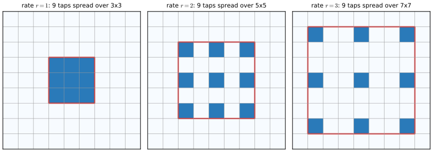
Filling the gap 14.11: dilated convolution is a convolution with a zero-inserted filter; receptive fields with dilations \(1,2,4,\dots\) pp. 486–487, (14.25)
Derivation
Equivalence. Define \(\tilde w_{u',v'}=w_{u,v}\) if \(u'=ru\) and \(v'=rv\), and \(0\) otherwise, for \(0\le u',v'\le r(k-1)\) (size \(r(k-1)+1\)). Then \(\sum_{u',v'}\tilde w_{u'v'}x_{i+u',j+v'}=\sum_{u,v}w_{uv}x_{i+ru,j+rv}\), which is (14.25) for one channel. The dilated layer has the \(k^2CD\) parameters of the small filter, but each unit sees \(r(k-1)+1\) pixels per side; with padding \(p=r(k-1)/2\) the output has the input's size. With the output-size formula of Gap 14.3, the output length is \(\lfloor(n+2p-r(k-1)-1)/s\rfloor+1\). Numerically, for \(r=1,2,3\) the dilated convolution equals the convolution with the zero-inserted filter to machine precision.
Receptive field of a stack. By the recursion of Gap 14.6 with stride 1: \(R_L=1+\sum_{l=1}^Lr_l(k-1)\). With \(k=3\) and rates \(r_l=2^{l-1}\): \(R_L=1+2(2^L-1)=2^{L+1}-1\), i.e. 3, 7, 15, 31, ... for \(L=1,2,3,4\), whereas \(L\) undilated \(3\times3\) layers give only \(2L+1\); so the field grows exponentially with depth while the number of parameters and the resolution stay fixed (Figure 14.S3). This is the reason it is used in segmentation encoders and in audio models. One caveat: with a constant rate \(r>1\) and stride 1, the taps of successive layers lie on the same sublattice, so some input pixels are never used ("gridding"); using rates that grow without a common factor (for example \(1,2,5\)) avoids this. \(\square\)
14.4.2 Transposed convolution
pp. 486–488 Convolution maps a large input to a smaller output. Transposed convolution goes the other way: every input pixel stamps a copy of the kernel, scaled by the pixel's value, onto a larger output and the copies are added (the book's trans_conv; for an \(h\times w\) kernel and an \(m\times n\) input the output is \((m+h-1)\times(n+w-1)\)). The name comes from the matrix form of Section 14.2.1.3: with \(\bm C\) the matrix derived from the kernel, the transposed convolution is \(\bm Y=\operatorname{reshape}(\bm C^\T\vecop(\bm X))\) (Figure 14.24). It is often called deconvolution, which is a misnomer: deconvolution undoes a known convolution, for example a blur, to recover the input (Figure 14.25).
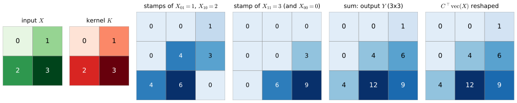
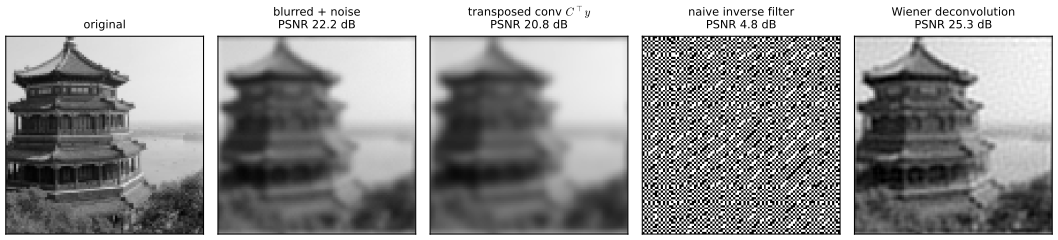
Filling the gap 14.12: the transposed convolution is the adjoint \(\bm C^\T\); output size; checkerboards; deconvolution is different pp. 486–488 ("one can show")
Derivation
Claim. Let \(\bm C\) be the matrix of the valid cross-correlation of an \(M\times N\) image with the kernel \(\bm K\) (\(h\times w\)), so \(\bm C\in\R^{(M-h+1)(N-w+1)\times MN}\). Then for an input \(\bm X\) of size \((M-h+1)\times(N-w+1)\), the book's trans_conv\((\bm X,\bm K)\) equals \(\operatorname{reshape}(\bm C^\T\vecop(\bm X))\), an \(M\times N\) array.
Proof. By Gap 14.2, \(C_{\omega(i,j),\iota(a,b)}=\sum_{u,v}K_{uv}\ind\{a=i+u,b=j+v\}\). Hence \((\bm C^\T\vecop\bm X)_{\iota(a,b)}=\sum_{i,j}C_{\omega(i,j),\iota(a,b)}X_{ij}=\sum_{i,j}\sum_{u,v}K_{uv}X_{ij}\ind\{a=i+u,b=j+v\}\), i.e. \(Y_{ab}=\sum_{i,j}X_{ij}K_{a-i,b-j}\) (with \(K\) zero outside its support). This is exactly what the book's loop computes: each \(X_{ij}\) adds \(X_{ij}K_{uv}\) at position \((i+u,j+v)\). It is also the full convolution of \(\bm X\) with \(\bm K\) (Gap 14.1) and its size is \((m+h-1)\times(n+w-1)\) for an \(m\times n\) input. (Confirmed numerically for random shapes, and against a library's transposed convolution.)
Why it is the natural "reverse" layer. (i) Adjoint: \(\langle\bm C\bm x,\bm y\rangle=\langle\bm x,\bm C^\T\bm y\rangle\) for all \(\bm x,\bm y\), so the transposed layer is the one that carries gradients backward through a convolution: if \(\bm y=\bm C\bm x\) and \(\bm g=\partial L/\partial\bm y\), then \(\partial L/\partial\bm x=\bm C^\T\bm g\). Backpropagation through a conv layer is therefore a transposed convolution. (ii) Shapes: it maps the output space of the convolution back to its input space, so up-sampling decoders use it to return to the input resolution.
Output size with stride and padding. A stride-\(s\), padding-\(p\) convolution on length \(n\) gives \(m=\lfloor(n+2p-k)/s\rfloor+1\) outputs (Gap 14.3). The transposed layer maps back from \(m\), producing \((m-1)s-2p+k\) outputs (the stride now spaces the stamps \(s\) pixels apart); this equals \(n\) when \(s\) divides \(n+2p-k\), and otherwise the original \(n\) is recovered only up to \(s-1\) pixels (libraries add an "output padding" argument to disambiguate). Checked against a library for several \((n,k,s,p)\).
Checkerboard artefacts. With stride \(s\) and kernel size \(k\), an output pixel receives contributions from \(\lceil k/s\rceil\) or \(\lfloor k/s\rfloor\) input pixels per dimension, depending on its position modulo \(s\); if \(s\nmid k\) the overlap is uneven, producing a periodic pattern with period \(s\) even for a constant kernel and input. The demonstration shows it for \(k=3\), \(s=2\).
Deconvolution is a different problem. For circular boundary conditions the convolution with kernel \(\bm K\) acts in Fourier space as multiplication by \(\hat K(\bm\omega)\) (Gap 14.2). The transposed convolution multiplies by \(\overline{\hat K(\bm\omega)}\) instead, so \(\bm C^\T\bm C\) has the transfer function \(|\hat K|^2\), a second blur, not the identity. An inverse filter divides by \(\hat K\): exact without noise, but with noise of variance \(\sigma^2\) the error at frequency \(\bm\omega\) has variance \(\sigma^2/|\hat K(\bm\omega)|^2\), enormous where \(|\hat K|\) is small (Gaussian blurs have \(|\hat K|\to0\) at high frequencies). The Wiener filter \(\overline{\hat K}/(|\hat K|^2+\lambda)\) is the Tikhonov-regularised solution of \(\min_{\bm x}\|\bm C\bm x-\bm y\|^2+\lambda\|\bm x\|^2\): at frequencies with \(|\hat K|^2\gg\lambda\) it inverts, at those with \(|\hat K|^2\ll\lambda\) it suppresses. In Figure 14.25 the three treatments differ by 20 dB. \(\square\)
14.4.3 Depthwise separable convolution
p. 488 A standard convolution with a filter of size \(H\times W\times C\times D\) is expensive. A depthwise separable convolution first convolves each input channel with its own 2-d filter, then maps the \(C\) channels to \(D\) by a \(1\times1\) convolution: \[ z_{i,j,d}=b_d+\sum_{c=0}^{C-1}w'_{c,d}\Big(\sum_{u=0}^{H-1}\sum_{v=0}^{W-1}x_{i+u,\,j+v,\,c}\,w_{u,v,c}\Big). \tag{14.26} \] In the book's example a \(12\times12\times3\) input and a \(5\times5\times3\times256\) filter give an \(8\times8\times256\) output with \(5\cdot5\cdot3\cdot256=19{,}200\) weights; the separable version (\(5\times5\) filter per channel, \(3\to256\) pointwise) gives the same output size with far fewer weights and multiplications. It is the basis of lightweight models such as MobileNet.
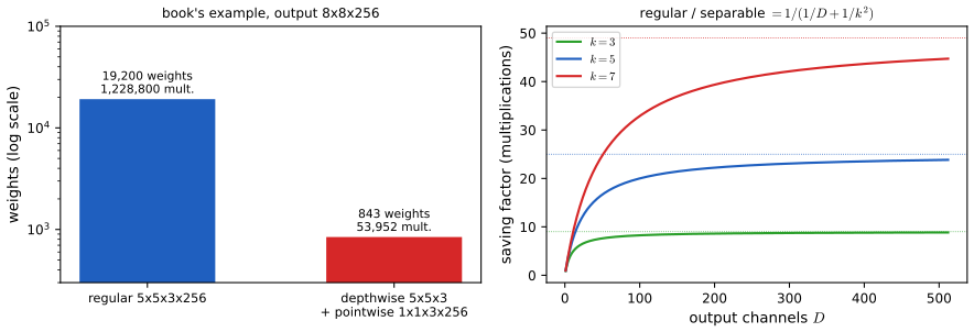
Filling the gap 14.13: parameter and multiplication counts of depthwise separable convolution, and what it assumes p. 488, (14.26)
Derivation
Counts. Regular: weights \(k^2CD\); output \(H_{\rm o}\times W_{\rm o}\times D\), each output a dot product of length \(k^2C\), so \(H_{\rm o}W_{\rm o}Dk^2C\) multiplications. Separable: depthwise stage \(k^2C\) weights and \(H_{\rm o}W_{\rm o}Ck^2\) multiplications (one \(k\times k\) dot product per channel and position); pointwise stage \(CD\) weights and \(H_{\rm o}W_{\rm o}CD\) multiplications; total \(k^2C+CD\) weights and \(H_{\rm o}W_{\rm o}C(k^2+D)\) multiplications. The ratio is \[ \frac{k^2CD}{k^2C+CD}=\frac{k^2D}{k^2+D}=\frac1{1/D+1/k^2}. \] Book example: \(k=5,C=3,D=256,H_{\rm o}=W_{\rm o}=8\) (valid: \(12-5+1\)): regular \(19{,}200\) weights and \(64\cdot19{,}200=1{,}228{,}800\) multiplications; separable \(75+768=843\) weights and \(64\cdot3\cdot(25+256)=53{,}952\) multiplications; ratios \(22.8\) in both (the multiplications ratio is \(25\cdot256/281=22.78\)). The saving tends to \(k^2\) as \(D\to\infty\).
What it assumes. Written as a 4-d filter \(w^{\rm sep}_{u,v,c,d}=w_{u,v,c}\,w'_{c,d}\): the separable layer is the subset of regular layers whose filter bank factorises over (space, channel) for each input channel, i.e. for each \(c\) the matrix \((w_{u,v,c,d})_{(uv),d}\) has rank 1. It is therefore a restriction, a low-rank structure, not an equivalent re-parametrisation; with the same \(C,D\) it cannot represent every regular convolution, but with a bit more width and the two nonlinearities (one after each stage in MobileNet) it works well in practice. The implementation with a "grouped convolution with \(C\) groups" followed by a \(1\times1\) convolution equals the formulas above (confirmed against a library). \(\square\)
14.5 Solving other discriminative vision tasks with CNNs
pp. 488–493 Each task below keeps the CNN body and changes the output layer or adds one architectural idea.
14.5.1 Image tagging
pp. 488–489 Classification assumes exactly one label per image. In image tagging (multi-label prediction) several tags may apply, so the output space is \(\mathcal Y=\{0,1\}^C\) and, since the bits are modelled as independent given the image, the final softmax is replaced by \(C\) logistic units. User-created hashtags give a cheap source of labels for pretraining (Mahajan et al., 2018) although they are noisy. The book notes that tagging is often a more sensible objective than classification because many images contain several objects: it quotes the author of the human-performance benchmark on ImageNet, who attributed about 16% of human errors to images with several classes where it is unclear which one is meant. The likelihood and why softmax cannot do this are in Gap 14.14.
Filling the gap 14.14: the multi-label likelihood and its gradient; softmax versus independent sigmoids p. 488
Derivation
Let the network output logits \(a_1,\dots,a_C\) and model \(p(\bm y\given\bm x)=\prod_{c=1}^C\operatorname{Ber}(y_c\given\sigma(a_c))\). The negative log-likelihood of one example is \[ \NLL=-\sum_{c=1}^C\big[y_c\log\sigma(a_c)+(1-y_c)\log(1-\sigma(a_c))\big]=\sum_{c=1}^C\big[\log(1+e^{a_c})-y_ca_c\big], \] because \(-\log\sigma(a)=\log(1+e^{-a})=\log(1+e^{a})-a\) and \(-\log(1-\sigma(a))=\log(1+e^{a})\) (\(\sigma(-a)=1-\sigma(a)\)). It is a sum of \(C\) binary cross entropies (checked numerically). Differentiating, \(\partial\NLL/\partial a_c=\sigma(a_c)-y_c\), the same "prediction minus target" as for logistic regression (Section 10.2.3); backpropagation continues as before.
Softmax cannot represent two labels. With a softmax the probabilities satisfy \(\sum_cp_c=1\), so two classes can both have probability near 1 only if the model were allowed to exceed 1. The best a softmax can do for an image whose true tags are "cat" and "dog" is \(p_{\rm cat}=p_{\rm dog}=\tfrac12\) (minimising \(-\tfrac12\log p_{\rm cat}-\tfrac12\log p_{\rm dog}\)), and the tags are mutually exclusive by construction. Independent sigmoids give each class its own probability in \([0,1]\); the price is the conditional-independence assumption: given \(\bm x\), knowing that "dog" is present does not change \(p(\text{leash}\given\bm x)\) beyond what \(\bm x\) says. If tag co-occurrence matters one can add structure (for example a conditional random field over tags). \(\square\)
14.5.2 Object detection
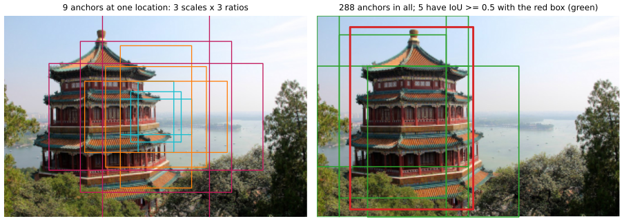
pp. 489–490 Object detection returns a variable number of bounding boxes with class labels (face detection is the one-class case; it differs from face recognition, which is classification of a detected face). It is an open-world problem, converted into a closed-world one with a finite set of anchor boxes at several locations, scales and aspect ratios (Figure 14.27b). The network learns \[ f_\theta:\R^{H\times W\times K}\to[0,1]^{A\times A}\times\{1,\dots,C\}^{A\times A}\times(\R^4)^{A\times A}, \tag{14.27} \] which for every anchor location \((i,j)\) gives an object probability \(p_{ij}\), a class \(y_{ij}\) and an offset \(\bm\delta_{ij}\in\R^4\) that is added to the anchor to obtain the corners of the predicted box (residual regression allows sub-grid localisation). Examples are the single-shot detector (Liu et al., 2016) and YOLO (Redmon et al., 2016).
Filling the gap 14.15: intersection over union, anchors, and why offsets are measured relative to the anchor pp. 489–490, (14.27)
Derivation
IoU. For two boxes \(A,B\subset\R^2\), \(\IoU(A,B)=|A\cap B|/|A\cup B|=|A\cap B|/(|A|+|B|-|A\cap B|)\). For axis-aligned boxes \((x_0,y_0,x_1,y_1)\), \(|A\cap B|=\max(0,\min(x_1,x_1')-\max(x_0,x_0'))\cdot\max(0,\min(y_1,y_1')-\max(y_0,y_0'))\). Properties: \(0\le\IoU\le1\); \(\IoU=1\) iff \(A=B\) (up to null sets); \(\IoU=0\) iff the interiors are disjoint. Example: two \(2\times2\) boxes overlapping in a \(1\times1\) square have \(\IoU=1/(4+4-1)=1/7\). \(d_J=1-\IoU\) is the Jaccard distance, a metric on measurable sets of finite measure (Marczewski and Steinhaus, 1958; the triangle inequality \(d_J(A,C)\le d_J(A,B)+d_J(B,C)\) is the non-trivial part and is quoted here). \(\IoU\) is invariant to translating and to scaling both boxes by the same factor: if \(A\mapsto\lambda A+\bm t\) and \(B\mapsto\lambda B+\bm t\) then all areas scale by \(\lambda^2\) and the ratio does not change. A loss on box coordinates (squared distance of corners) has no such invariance: the same relative error costs \(\lambda^2\) times more for a larger object.
Anchors and positives. A grid of \(A\times A\) locations with \(S\) scales and \(R\) ratios has \(A^2SR\) anchors (Figure 14.27b: \(4\cdot6\cdot4\cdot3=288\)); an anchor of scale \(s\) and ratio \(r=w/h\) has width \(s\sqrt r\,\ell\) and height \(s\ell/\sqrt r\) (\(\ell\) a reference length), hence area \(s^2\ell^2\) independent of \(r\). A ground-truth box is matched to the anchors with \(\IoU\ge\tau\) (0.5 is common), which are trained to predict it; the rest are trained as "background". Typical per-anchor loss: cross entropy for object presence and class plus a robust regression loss on the offsets of positive anchors only.
Relative offsets. If the anchor has centre \((x_a,y_a)\) and size \((w_a,h_a)\), parametrising the target by \(t_x=(x-x_a)/w_a\), \(t_y=(y-y_a)/h_a\), \(t_w=\log(w/w_a)\), \(t_h=\log(h/h_a)\) makes the targets dimensionless and approximately of the same size for all scales, and \(\IoU\) of the decoded box depends only on the \(\bm t\) (by the invariance above): the regression problem is the same at every scale, which is why it is learned with one set of shared weights (Ren et al., 2015, quoted; the argument here is only the scale invariance). The book's \(\bm\delta\) "added to the centroid to get the corners" is the same idea with a linear parametrisation. At test time many anchors fire on one object, which is cleaned by non-maximum suppression: keep the highest-scoring box and discard the boxes whose IoU with it exceeds a threshold, repeat. \(\square\)
See also: Foundations of Deep Learning, 10.4.2 intersection-over-union and 10.4.5 non-max suppression.
14.5.3 Instance segmentation
pp. 490–491 Instance segmentation predicts, for each object instance, its label and a pixel mask (Figure 14.28, a photograph of Mask R-CNN output). It can be done by running a semantic-segmentation network inside every detected box, deciding for each pixel whether it belongs to the object (foreground) or not.
14.5.4 Semantic segmentation
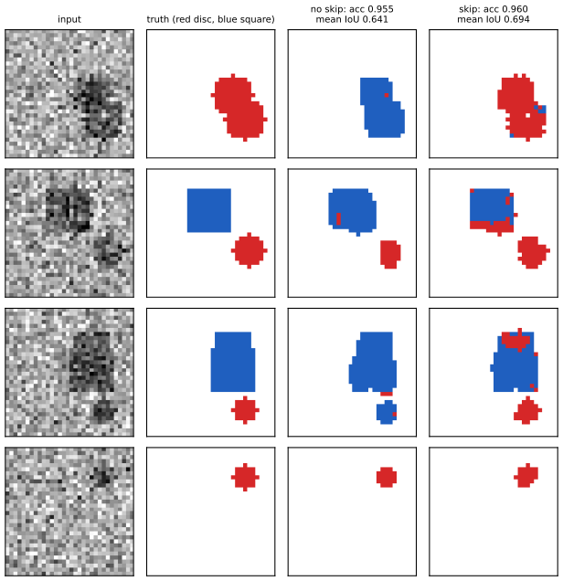
pp. 491–492 In semantic segmentation every pixel \(i\) gets a class \(y_i\in\{1,\dots,C\}\); all pixels of a class share the label whatever the instance. Combining semantic segmentation of "stuff" (sky, road) and instance segmentation of "things" (cars, people) gives panoptic segmentation. A common architecture is an encoder-decoder (Figure 14.29): the encoder uses convolution and down-sampling (often dilated convolution, Section 14.4.1, for context) to a small bottleneck, the decoder up-samples back with transposed convolution (Section 14.4.2); skip connections from encoder to decoder restore the detail lost in the bottleneck. Drawn out, the shape is a U, hence U-net (Ronneberger et al., 2015; Figure 14.30). The same architecture, with other output heads, gives depth, surface-normal and other dense predictions, trained jointly with multiple heads (Figure 14.31).
Filling the gap 14.16: the per-pixel loss, the size bookkeeping of the U-net of Figure 14.30, and what skip connections add pp. 491–492, Figures 14.29–14.30
Derivation
Loss. The network outputs \(C\) logits at each pixel \(i\in\Omega\), giving \(p_i(c\given\bm x)=\softmax(\bm a_i)_c\). If the pixels are modelled as conditionally independent given the image (the network, not the likelihood, carries the spatial correlation), the NLL is \(-\sum_{i\in\Omega}\log p_i(y_i\given\bm x)\): \(|\Omega|\) classification problems that share the network (with a \(1\times1\) convolution as the last layer, Gap 14.4); the gradient at the logits is \(\bm p_i-\bm e_{y_i}\) as in multinomial logistic regression (Section 10.3). Class imbalance (most pixels are background) is handled by class weights or an overlap-based loss.
Sizes in Figure 14.30. Each \(3\times3\) "valid" convolution removes 2 pixels per dimension (Gap 14.3); each level has two, so \(n\mapsto n-4\); \(2\times2\) max pooling halves (the size must be even); the \(2\times2\) up-convolution doubles. Starting from \(572\): encoder \(568\to284\) (pool) \(\to280\to140\to136\to68\to64\to32\to28\) at the bottleneck (\(1024\) channels in the figure); decoder \(2\cdot28=56\to52\), \(2\cdot52=104\to100\), \(2\cdot100=200\to196\), \(2\cdot196=392\to388\). The output is \(388\times388\), smaller than the \(572\times572\) input by 184 pixels: because the valid convolutions lose a border, the output segmentation only covers the central part of the input, and large images are processed in overlapping tiles ("overlap-tile strategy"). The encoder feature maps copied across are larger than the decoder maps at the same level (e.g. 64 against 56) and are centre-cropped before concatenation (the "copy and crop" arrows). With "same" padding all sizes stay powers of two multiples of the input and nothing is cropped.
What the skip connections add. A bottleneck of \(1/16\) of the resolution cannot encode the exact position of an edge, so the decoder's outputs are blurry at object boundaries; concatenating the high-resolution encoder features with the up-sampled ones lets the last layers refine boundaries. In the toy experiment of Figure 14.S4 (discs and squares in noise), the network with skip connections reaches a mean IoU of 0.69 against 0.64 without (pixel accuracy 96.0% against 95.5%; it also has more parameters, 56,723 against 45,203, because the decoder convolutions see the concatenated channels). Concatenation (as in DenseNet) rather than addition lets the decoder learn how to combine the two sources. \(\square\)
14.5.5 Human pose estimation
pp. 492–493 One can train a detector to find people and their masks, or to predict the positions of a fixed set of skeletal keypoints (head, hands, ...): human pose estimation (PersonLab, Papandreou et al., 2018; OpenPose, Cao et al., 2018; Figure 14.32). Three-dimensional properties of objects are also predicted, but labelled 3-d data are scarce because people cannot annotate in 3-d, so simulated images from graphics engines with exact ground truth are used.
14.6 Generating images by inverting CNNs
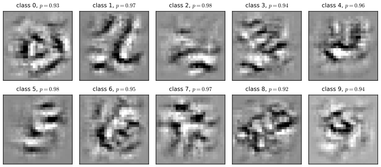
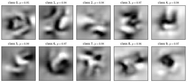
p. 493 A classifier is a discriminative model \(p(y\given\bm x)\). This section "inverts" it into a conditional generative model \(p(\bm x\given y)\) so that images of a given class can be generated, and then uses the same machinery for visualising the features a network has learned, DeepDream and style transfer. The book points to its sequel for principled generative models of images. To keep the images small and reproducible, all the computed figures in this section use a small CNN (two \(5\times5\) convolutions with 6 and 12 channels, ReLU, \(2\times2\) max pooling after each, one dense layer, 3,898 parameters) trained for three epochs on 20,000 MNIST digits, with 97.8% accuracy on the 10,000 test digits; the book's figures use ImageNet networks.
14.6.1 Converting a trained classifier into a generative model
pp. 493–494 A joint model is \(p(\bm x,y)=p(\bm x)p(y\given\bm x)\) with \(p(y\given\bm x)\) the CNN and \(p(\bm x)\) a prior over images. Clamping \(y=c\) gives \[ p(\bm x\given y=c)\propto p(\bm x)\,p(y=c\given\bm x). \] The classifier was trained to discard information, so it is not invertible and the prior \(p(\bm x)\) matters. One can sample by Metropolis-Hastings (Section 4.6.8.4) with the log of the unnormalised density as the "energy", and since gradients are available use the Langevin proposal \(q(\bm x'\given\bm x)=\N(\bm\mu(\bm x),\epsilon\bm I)\) with \(\bm\mu(\bm x)=\bm x+\frac\epsilon2\nabla\mathcal E_c(\bm x)\), \(\mathcal E_c(\bm x)=\log p(y=c\given\bm x)+\log p(\bm x)\): the Metropolis-adjusted Langevin algorithm (MALA). Ignoring the accept-reject step gives the unadjusted Langevin algorithm, used by Nguyen et al. (2017). Scaling the prior and likelihood terms separately gives the noisy gradient ascent on the pixels \[ \bm x_{t+1}=\bm x_t+\epsilon_1\frac{\partial\log p(\bm x_t)}{\partial\bm x_t}+\epsilon_2\frac{\partial\log p(y=c\given\bm x_t)}{\partial\bm x_t}+\mathcal N(\bm 0,\epsilon_3^2\bm I), \tag{14.28} \] where the derivatives with respect to the input pixels are computed by backpropagation (Equation 13.50): \(\epsilon_1\) keeps the image plausible under the prior, \(\epsilon_2\) makes it plausible under the classifier and \(\epsilon_3\) gives diversity. With \(\epsilon_3=0\) it is a deterministic search for the (approximately) most likely image of the class.
Filling the gap 14.17: why Langevin updates target \(p(\bm x\given y)\); the bias of the unadjusted algorithm; the Metropolis correction; what (14.28) really optimises pp. 493–494, (14.28)–(14.30)
Derivation
Langevin diffusion. Let \(\pi(\bm x)\propto e^{-U(\bm x)}\) be a smooth density (here \(\pi=p(\bm x\given y=c)\), \(U=-\log p(\bm x)-\log p(y=c\given\bm x)+\mathrm{const}\)). The diffusion \(\d\bm X_t=\tfrac12\nabla\log\pi(\bm X_t)\,\d t+\d\bm B_t\) has \(\pi\) as an invariant density: its Fokker-Planck equation is \(\partial_t\rho=-\nabla\cdot(\tfrac12\rho\nabla\log\pi)+\tfrac12\Delta\rho=\tfrac12\nabla\cdot\big(\nabla\rho-\rho\nabla\log\pi\big)\), and for \(\rho=\pi\) we have \(\nabla\pi=\pi\nabla\log\pi\), so the bracket vanishes and \(\partial_t\rho=0\). The Euler discretisation with step \(\epsilon\) is \[ \bm x_{t+1}=\bm x_t+\frac\epsilon2\nabla\log\pi(\bm x_t)+\sqrt\epsilon\,\bm\xi_t,\qquad\bm\xi_t\sim\N(\bm 0,\bm I), \] the proposal of MALA with mean \(\bm\mu(\bm x)=\bm x+\frac\epsilon2\nabla\log\pi(\bm x)\) and covariance \(\epsilon\bm I\). Since \(\nabla\log\pi=\nabla\log p(\bm x)+\nabla\log p(y=c\given\bm x)\), the update is (14.28) with \(\epsilon_1=\epsilon_2=\epsilon/2\) and \(\epsilon_3=\sqrt\epsilon\). If one uses \(\epsilon_1=\frac\epsilon2a\) and \(\epsilon_2=\frac\epsilon2b\) the same algebra targets \(\pi_{a,b}\propto p(\bm x)^a\,p(y=c\given\bm x)^b\): a re-weighted (tempered) posterior, which is what the "scale the gradients independently" remark of the book does; with \(\epsilon_3=0\) it is gradient ascent on \(a\log p(\bm x)+b\log p(y=c\given\bm x)\), a MAP image.
The unadjusted algorithm is biased. For \(\pi=\N(0,1)\), \(\nabla\log\pi(x)=-x\) and the update is the AR(1) recursion \(x'=(1-\epsilon/2)x+\sqrt\epsilon\xi\). Its stationary variance \(v\) solves \(v=(1-\epsilon/2)^2v+\epsilon\), so \(v=\epsilon/(\epsilon-\epsilon^2/4)=1/(1-\epsilon/4)>1\): the chain samples \(\N(0,1/(1-\epsilon/4))\), not \(\pi\); the bias vanishes only as \(\epsilon\to0\) (for \(\epsilon=0.2\), \(v=1.0526\); a simulation with \(4\times10^5\) independent chains gives 1.049). Dropping the accept-reject step therefore changes the target slightly, which does not matter for generating images.
Metropolis adjustment. Accept the proposal \(\bm x'\) with probability \(\alpha=\min\!\big(1,\frac{\pi(\bm x')q(\bm x\given\bm x')}{\pi(\bm x)q(\bm x'\given\bm x)}\big)\). Because \(q\) is Gaussian, \(\log\frac{q(\bm x\given\bm x')}{q(\bm x'\given\bm x)}=-\frac1{2\epsilon}\big(\|\bm x-\bm\mu(\bm x')\|^2-\|\bm x'-\bm\mu(\bm x)\|^2\big)\) is cheap given the gradients at \(\bm x\) and \(\bm x'\). By detailed balance (Section 4.6.8.4) \(\pi\) is then exactly invariant; for the same Gaussian target and \(\epsilon=0.5\), \(4\times10^5\) chains give variance 0.999 (simulation).
Priors in the update. For the prior \(p(\bm x)=\N(\bm 0,\bm I)\), \(\nabla_{\bm x}\log p=-\bm x\) (14.29), so with \(\epsilon_2=1\), \(\epsilon_3=0\) the update is \(\bm x_{t+1}=(1-\epsilon_1)\bm x_t+\partial\log p(y=c\given\bm x_t)/\partial\bm x_t\) (14.30). For a fixed point \(\bm x^\star\) we need \(\epsilon_1\bm x^\star=\epsilon_2\nabla\log p(y=c\given\bm x^\star)\): the pull of the prior balances the push of the classifier. This is "weight decay on the pixels"; Exercise 14.6 solves it for a logistic classifier. Without a prior (\(\epsilon_1=0\)) nothing bounds the pixels: along the ascent direction the classifier's logit margin grows without limit (the "adversarial" or "fooling image" regime of Figures 14.33 and the demonstration, preset 3).
All gradients with respect to the pixels in the code are computed by hand-written backpropagation through convolution, ReLU and max pooling and match automatic differentiation. \(\square\)
See also: Foundations of Deep Learning, 14.3.3 Langevin dynamics; Bayesian and Probabilistic ML, 11.2.2 the Metropolis-Hastings algorithm; adversarial examples (FGSM) demo.
14.6.2 Image priors
pp. 494–495 The class label alone does not specify the kind of image wanted; the prior \(p(\bm x)\) regularises this ill-posed problem, and together with the starting image it determines the output.
14.6.2.1 Gaussian prior
The simplest prior is \(p(\bm x)=\N(\bm x\given\bm 0,\bm I)\) (for centred pixels; Simonyan et al., 2014), which prevents extreme pixel values: \(\nabla_{\bm x}\log p(\bm x)=-\bm x\) (14.29), and with \(\epsilon_2=1\), \(\epsilon_3=0\) the update is \(\bm x_{t+1}=(1-\epsilon_1)\bm x_t+\partial\log p(y=c\given\bm x_t)/\partial\bm x_t\) (14.30). Figure 14.33 shows images generated this way.
14.6.2.2 Total variation (TV) prior
pp. 494–495 Slightly more realistic images result from penalising high-frequency content with the total variation (Mahendran and Vedaldi, 2015, 2016), \[ \TV(\bm x)=\sum_{i,j,k}\big[(x_{ijk}-x_{i+1,j,k})^2+(x_{ijk}-x_{i,j+1,k})^2\big]=\sum_k\|\bm H(\bm x_{:,:,k})\|_F^2+\|\bm V(\bm x_{:,:,k})\|_F^2, \tag{14.31, 14.32} \] where \(\bm H\) and \(\bm V\) apply the horizontal and vertical difference filters (the book says Sobel filters; see the notes on the book) to channel \(k\), and with \(p(\bm x)\propto e^{-\TV(\bm x)}\) (Figure 14.34). Yosinski et al. (2015) use a Gaussian blur instead, with a similar effect. Figure 14.35 shows class-conditional images from a TV prior and the CNN likelihood.

Filling the gap 14.18: what the TV penalty (14.31) is, its gradient and why it smooths pp. 494–495, (14.29), (14.31)–(14.32)
Derivation
The quantity. The sum of squared neighbouring differences over the \(H\times W\) grid is the quadratic form \(\bm x^\T\bm L\bm x\) with \(\bm L\) the graph Laplacian of the grid (\(\bm L=\bm D-\bm A\)): \(\sum_{(i,j)\sim(i',j')}(x_{ij}-x_{i'j'})^2=\bm x^\T\bm L\bm x\), the standard identity for a sum over edges. It is the discrete Dirichlet energy \(\int\|\nabla x\|^2\), not the total variation \(\int\|\nabla x\|\) (without the square), which is the \(\ell_1\)-type penalty that preserves edges in the Rudin-Osher-Fatemi denoising model. The squared version is what the book writes in (14.31), and (14.32) restates it with the difference filters \(\bm H=(1,-1)\) and \(\bm V=(1,-1)^\T\): \(\sum\|\bm H\bm X\|_F^2+\|\bm V\bm X\|_F^2\) (confirmed numerically); these are finite differences, not the Sobel filters (which also smooth in the perpendicular direction). The name "total variation" is kept for continuity with the literature.
Gradient. \(\nabla_{\bm x}(\bm x^\T\bm L\bm x)=2\bm L\bm x\), where \((\bm L\bm x)_{ij}=\sum_{\text{neighbours}}(x_{ij}-x_{i'j'})\): twice minus the discrete Laplacian. The gradient formula agrees with finite differences. The prior gradient is \(\nabla\log p(\bm x)=-2\lambda\bm L\bm x\) and the prior part of the update is \(\bm x\leftarrow\bm x-2\epsilon_1\lambda\bm L\bm x\), an explicit step of the heat equation \(\partial_t\bm x=-\bm L\bm x\), which is a low-pass filter: in the Fourier basis of the grid, \(\bm L\) has eigenvalues \(\mu_{\bm\omega}=4-2\cos\omega_1-2\cos\omega_2\in[0,8]\) (for a periodic grid), and every step multiplies the component at frequency \(\bm\omega\) by \(1-2\epsilon_1\lambda\mu_{\bm\omega}\): the constant mode (\(\mu=0\)) is untouched and high frequencies are damped by up to \(1-16\epsilon_1\lambda\) per step. The classifier's gradient keeps adding the detail that raises \(p(y=c\given\bm x)\), and the prior removes what is oscillatory: the equilibrium is a smooth image. This explains the blobby look of Figure 14.35 compared with Figure 14.33.
Stability of the update. The explicit step is stable only if \(|1-2\epsilon_1\lambda\mu|\le1\) for \(\mu\le8\), i.e. \(\epsilon_1\lambda\le1/8\); with \(\epsilon_1=0.05\), \(\lambda=0.5\) the factor at the highest frequency is \(1-16\cdot0.025=0.6\), so the prior step is stable (the likelihood step is added to it).
Gaussian prior. By (14.29) the Gaussian prior multiplies every pixel by \(1-\epsilon_1\) per step: a ridge penalty on the pixel values; it shrinks the norm, not the roughness, which is why Figure 14.33 stays speckled. \(\square\)
14.6.3 Visualizing the features learned by a CNN
p. 495 To ask what a hidden unit has learned, start from a random image and optimise the pixels so as to maximise the mean activation of that unit: activation maximisation, the method of 14.6.1 with an internal node fixed instead of the class label. Figure 14.36 in the book (AlexNet, TV prior; Mahendran and Vedaldi, 2016) shows that units in deeper layers respond to edges and blobs, then textures, then object parts, then whole objects, roughly like the hierarchy of the visual cortex. An alternative is to search the training set for images that activate the unit most (the "data driven" column for Conv5; Olah et al., 2017, review feature visualisation).
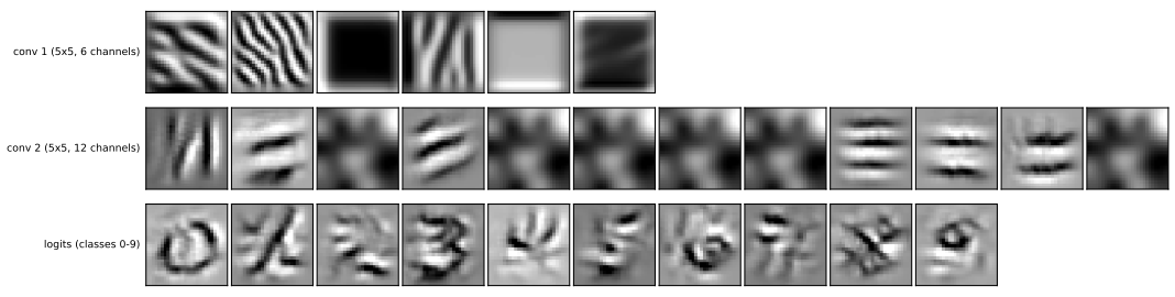
14.6.4 Deep Dream
pp. 496–497 Instead of maximising one unit or a class, treat a trained classifier as a feature extractor and amplify whatever the features of some layers \(\mathcal L\) already see in a given image. With \(\phi_l(\bm x)\) the average of layer \(l\)'s feature map, the energy is \(\mathcal L(\bm x)=\sum_{l\in\mathcal L}\phi_l(\bm x)\), optimised by gradient ascent: DeepDream (Mordvintsev et al., 2015; originally "Inceptionism"). Starting from a photograph (Figure 14.37) the result is a hybrid with the dog-like hallucinations of an ImageNet Inception network.
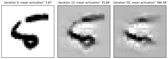
Filling the gap 14.19: why activation maximisation needs a prior or a constraint, the first-layer answer, and gradient ascent on the dream objective pp. 495–497
Derivation
Unbounded without a constraint. A ReLU network without biases is positively homogeneous of degree 1: \(\bm a(t\bm x)=t\,\bm a(\bm x)\) for \(t>0\), because \(\relu(tz)=t\relu(z)\) and linear maps commute with scalars (max pooling too). So for any unit with \(a_j(\bm x)>0\), \(a_j(t\bm x)\to\infty\) as \(t\to\infty\): the supremum of the activation over images is \(+\infty\) and "the image that maximises the unit" does not exist. (With biases the statement is asymptotic.) Any finite answer comes from the prior, a bound on the pixels, or early stopping, and different priors give different pictures; this is the reason the book needs a prior in Section 14.6.2 for the feature visualisations.
First layer. For a unit of the first convolution at one position, \(a=\bm w^\T\bm p+b\) with \(\bm p\) the \(5\times5\) patch. Under \(\|\bm p\|\le\rho\) the maximum is attained at \(\bm p=\rho\bm w/\|\bm w\|\) by Cauchy-Schwarz, i.e. the optimal stimulus is the filter, scaled. When one maximises the mean over all positions of a channel the patches overlap and the optimum is a pattern in which every patch resembles the filter, which gives the tiled stripes of Figure 14.36; so the first-layer pictures simply display the learned filters, as the hierarchy of the book's Figure 14.36 does.
Normalised gradient ascent. With a loss \(\mathcal L\) that has an \(L\)-Lipschitz gradient, a step \(\bm x\leftarrow\bm x+\eta\bm g\), \(\bm g=\nabla\mathcal L(\bm x)\), satisfies \(\mathcal L(\bm x+\eta\bm g)\ge\mathcal L(\bm x)+\eta\|\bm g\|^2-\tfrac L2\eta^2\|\bm g\|^2\) (the descent lemma applied to \(-\mathcal L\)), so \(\mathcal L\) increases for \(\eta<2/L\). DeepDream implementations divide the gradient by its mean absolute value, which makes the step size in pixel units independent of the layer's scale; the objective then increases for a small enough step (in the experiment from 3.9 to 36 in 10 steps and to 597 in 50), and the growth shows the instability described above: nothing bounds the energy, so one stops after a fixed number of iterations (and the images grow garish). The book defines the energy through averages of feature maps; the experiment uses the mean of the squared second-layer activations, a common choice that is positive and amplifies strong responses. \(\square\)
14.6.5 Neural style transfer
pp. 497–501 Given a content image \(\bm x_c\) and a style image \(\bm x_s\), neural style transfer (Gatys et al., 2016) generates \(\bm x\) that re-renders the content in the style (Figures 14.38, 14.39 and 14.40).
14.6.5.1 How it works
The pixels are found by minimising \[ \mathcal L(\bm x\given\bm x_s,\bm x_c)=\lambda_{\rm TV}\mathcal L_{\rm TV}(\bm x)+\lambda_c\mathcal L_{\rm content}(\bm x,\bm x_c)+\lambda_s\mathcal L_{\rm style}(\bm x,\bm x_s). \tag{14.33} \] The first term is the total-variation prior of Section 14.6.2.2. The content term compares feature maps \(\phi_\ell\) of a pre-trained CNN at a chosen layer \(\ell\), \[ \mathcal L_{\rm content}(\bm x,\bm x_c)=\frac1{C_\ell H_\ell W_\ell}\|\phi_\ell(\bm x)-\phi_\ell(\bm x_c)\|^2. \tag{14.34} \] Style is the statistical distribution of certain features; where they occur does not matter but their co-occurrence does (Figure 14.41: images 1 and 2 are similar in style because both have spiky green patches). To capture co-occurrence use the Gram matrix of the feature maps of layer \(\ell\), \[ G_\ell(\bm x)_{c,d}=\frac1{H_\ell W_\ell}\sum_{h=1}^{H_\ell}\sum_{w=1}^{W_\ell}\phi_\ell(\bm x)_{h,w,c}\,\phi_\ell(\bm x)_{h,w,d}, \tag{14.35} \] a \(C_\ell\times C_\ell\) matrix proportional to the uncentred covariance of the \(C_\ell\)-dimensional feature vectors over the \(H_\ell W_\ell\) positions, with the layer style loss and the total \[ \mathcal L^\ell_{\rm style}(\bm x,\bm x_s)=\|\bm G_\ell(\bm x)-\bm G_\ell(\bm x_s)\|_F^2,\qquad\mathcal L_{\rm style}(\bm x,\bm x_s)=\sum_{\ell\in\mathcal S}\mathcal L^\ell_{\rm style}(\bm x,\bm x_s). \tag{14.36, 14.37} \] Lower layers capture texture, higher layers object layout.
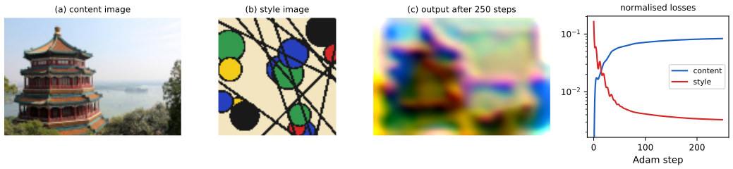
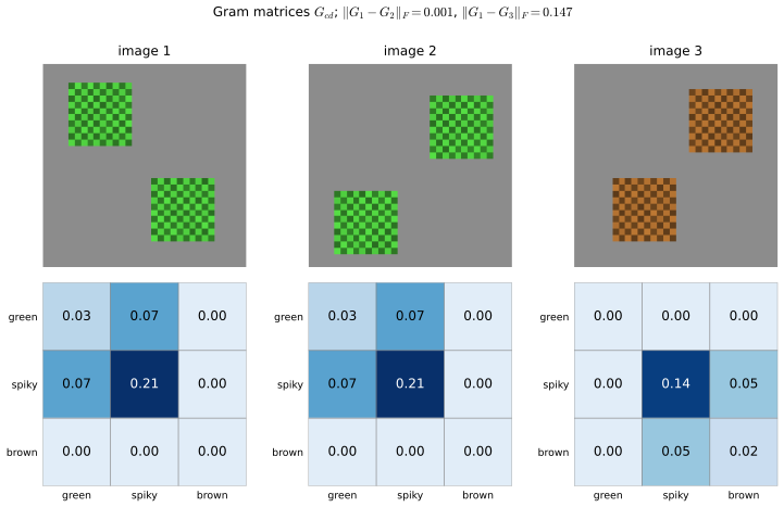
Filling the gap 14.20: the Gram matrix discards layout; the style loss is a kernel two-sample distance; its gradient pp. 497–500, (14.33)–(14.37)
Derivation
Write the feature map of a layer as a matrix \(\bm F\in\R^{C\times n}\) with \(n=HW\) (column \(\bm f_t\) the feature vector at position \(t\)); then \(\bm G=\frac1n\bm F\bm F^\T=\frac1n\sum_t\bm f_t\bm f_t^\T\) (14.35).
(i) \(\bm G\) is a positive semi-definite uncentred covariance. \(\bm v^\T\bm G\bm v=\frac1n\sum_t(\bm v^\T\bm f_t)^2\ge0\). The covariance would subtract the mean feature vector; \(\bm G=\operatorname{cov}+\bar{\bm f}\bar{\bm f}^\T\), so \(\bm G\) also carries first-order information.
(ii) Layout invariance. For any permutation matrix \(\bm\Pi\) of the \(n\) positions, \(\bm F\bm\Pi\) has Gram matrix \(\frac1n\bm F\bm\Pi\bm\Pi^\T\bm F^\T=\bm G\): shuffling the positions of the feature vectors, however drastically, leaves \(\bm G\) unchanged. This is the formal content of "the location of features may not matter, but their co-occurrence does" (verified for a random permutation, and visible in Figure 14.41). Because the convolutional features are local, the layer's receptive field still captures local structure, so local textures survive but global layout does not; deeper layers have larger receptive fields, which is why the style loss is summed over layers in (14.37).
(iii) The style loss is an MMD. Regard \(\{\bm f_t\}\) and \(\{\bm g_t\}\) (from the style image) as empirical distributions of feature vectors and use the polynomial kernel \(k(\bm a,\bm b)=(\bm a^\T\bm b)^2=\langle\bm a\bm a^\T,\bm b\bm b^\T\rangle_F\) with feature map \(\bm a\mapsto\bm a\bm a^\T\). The squared maximum mean discrepancy is \[ \mathrm{MMD}^2=\frac1{n^2}\sum_{s,t}k(\bm f_s,\bm f_t)-\frac2{nm}\sum_{s,t}k(\bm f_s,\bm g_t)+\frac1{m^2}\sum_{s,t}k(\bm g_s,\bm g_t)=\|\bm G_x\|_F^2-2\langle\bm G_x,\bm G_s\rangle+\|\bm G_s\|_F^2=\|\bm G_x-\bm G_s\|_F^2, \] because \(\frac1{n^2}\sum_{s,t}\langle\bm f_s\bm f_s^\T,\bm f_t\bm f_t^\T\rangle_F=\|\frac1n\sum_s\bm f_s\bm f_s^\T\|_F^2\) (Li et al., 2017). So (14.36) is exactly the squared MMD between the feature distributions of the output and the style image for a degree-2 polynomial kernel: style transfer matches the second moments of the feature distributions (verified numerically).
(iv) Gradient. With \(\bm G=\frac1n\bm F\bm F^\T\) and \(\mathcal L=\|\bm G-\bm G_s\|_F^2\): \(\d\mathcal L=2\langle\bm G-\bm G_s,\d\bm G\rangle\), \(\d\bm G=\frac1n(\d\bm F\,\bm F^\T+\bm F\,\d\bm F^\T)\), and since \(\bm G-\bm G_s\) is symmetric \(\d\mathcal L=\frac4n\langle(\bm G-\bm G_s)\bm F,\d\bm F\rangle\), i.e. \[ \frac{\partial\mathcal L^\ell_{\rm style}}{\partial\bm F}=\frac4{n}\,(\bm G-\bm G_s)\bm F, \] which is then backpropagated through the CNN to the pixels (the cost of one forward and one backward pass per step; confirmed against finite differences). The content loss (14.34) has gradient \(\frac2{CHW}(\phi_\ell(\bm x)-\phi_\ell(\bm x_c))\). The whole objective (14.33) is non-convex in \(\bm x\); Gatys et al. used L-BFGS from white noise, and initialising from the content image with Adam is faster (Section 14.6.5.2). \(\square\)
14.6.5.2 Speeding up the method
pp. 500–501 Running an optimiser per image pair is slow. A network \(f_s\) can be trained for each style so that \(f_s(\bm x_c)=\arg\min_{\bm x}\mathcal L(\bm x\given\bm x_s,\bm x_c)\): the optimisation is amortised (Johnson et al., 2016; Ulyanov et al., 2016; Li and Wand, 2016), and one forward pass replaces hundreds of gradient steps. Dumoulin et al. (2016) use a single network that also takes a discrete style \(s\) as input, with the conditional instance normalisation \[ \mathrm{CIN}(\phi(\bm x_c),s)=\gamma_s\,\frac{\phi(\bm x_c)-\mu(\phi(\bm x_c))}{\sigma(\phi(\bm x_c))}+\beta_s, \tag{14.38} \] where \(\mu,\sigma\) are the mean and standard deviation of the features of a layer (per channel, Section 14.2.4.2) and \(\gamma_s,\beta_s\) are parameters of style \(s\). Huang and Belongie (2017) allow an arbitrary style image by making the scale and shift outputs of another CNN of the style features, \(\beta_s=f_\beta(\phi(\bm x_s))\), \(\gamma_s=f_\gamma(\phi(\bm x_s))\), the adaptive instance normalisation \[ \mathrm{AIN}(\phi(\bm x_c),\phi(\bm x_s))=f_\gamma(\phi(\bm x_s))\,\frac{\phi(\bm x_c)-\mu(\phi(\bm x_c))}{\sigma(\phi(\bm x_c))}+f_\beta(\phi(\bm x_s)). \tag{14.39} \]
Filling the gap 14.21: what conditional and adaptive instance normalisation do to the statistics pp. 500–501, (14.38)–(14.39)
Derivation
Conditional instance normalisation. Fix an example and a channel and let \(\bm u=\phi(\bm x_c)_{:,:,c}\in\R^{HW}\). Instance normalisation (Section 14.2.4.2, \(S_i\) = the \(HW\) positions of this map) gives \(\hat{\bm u}=(\bm u-\mu)/\sigma\) with mean exactly \(0\) and, for \(\epsilon=0\), variance \(1\). Then (14.38) gives \(\tilde{\bm u}=\gamma_{s,c}\hat{\bm u}+\beta_{s,c}\) with mean \(\beta_{s,c}\) and standard deviation \(\gamma_{s,c}\) (for \(\gamma_{s,c}>0\)). Thus, in every layer, style \(s\) is encoded as a choice of the per-channel mean and standard deviation of the feature maps (a \(2C\)-dimensional vector per layer and style), and the image's own per-channel offsets and scales are erased, whatever the content image. That the network outputs a good stylised image from these few numbers shows that, in this family, a large part of what is called style is carried by first and second moments of the channels; it is a coarser statistic than the Gram matrix, which also holds the cross-channel products.
Adaptive instance normalisation. Choose \(f_\gamma(\phi(\bm x_s))=\sigma(\phi(\bm x_s))\) and \(f_\beta(\phi(\bm x_s))=\mu(\phi(\bm x_s))\), the per-channel standard deviation and mean of the style features. Then (14.39) is \(\sigma_s\frac{\bm u-\mu_c}{\sigma_c}+\mu_s\): a map with the style's mean \(\mu_s\) and standard deviation \(\sigma_s\) in every channel and the content map's shape otherwise (checked numerically). The book's version learns \(f_\gamma,f_\beta\), which can do this and more. The result does not depend on which style image was used beyond the \(2C\) numbers, so any style image can be used without retraining.
Amortisation. Training a feed-forward network \(f\) with the loss (14.33) on many content images (style fixed) solves the family of problems \(\arg\min_{\bm x}\mathcal L(\bm x\given\bm x_s,\bm x_c)\) simultaneously by minimising \(\E_{\bm x_c}[\mathcal L(f(\bm x_c)\given\bm x_s,\bm x_c)]\) over the weights of \(f\); at test time one forward pass replaces the optimisation. The learned \(f\) is only an approximation to the argmin for each \(\bm x_c\) and is trained on the training distribution of content images. \(\square\)
See also: Foundations of Deep Learning, 10.6 style transfer; 10.3.5 synthetic images.
14.7 Exercises
The book has no end-of-chapter exercises for Chapter 14 (the chapter ends with Section 14.6.5.2). To give the chapter the same practice material as the others, here are six exercises of my own, numbered 14.1 to 14.6 and not taken from the book, each with a complete worked solution (hidden); the computational ones were solved with the course code and the numbers checked.
Exercise 14.1 (shapes and parameters). A network takes a \(32\times32\times3\) image and applies: a \(5\times5\) convolution with 16 channels and padding 2, \(2\times2\) max pooling with stride 2, a \(3\times3\) convolution with 32 channels and padding 1, \(2\times2\) max pooling, global average pooling, and a dense layer with 10 outputs. Give the shape after each layer and the number of parameters. How many parameters would the dense layer need if one flattened the last feature map instead of pooling it globally?
Solution
Shapes (Gap 14.3): conv \(5\times5\), \(p=2\): \(32+4-5+1=32\), so \(32\times32\times16\); pool: \(16\times16\times16\); conv \(3\times3\), \(p=1\): \(16\times16\times32\); pool: \(8\times8\times32\); global average pool: \(32\); dense: \(10\). Parameters (\(k^2CD+D\)): \(25\cdot3\cdot16+16=1216\); \(9\cdot16\cdot32+32=4640\); pooling none; dense \(32\cdot10+10=330\); total \(6186\) (confirmed by a library count). With flattening the dense layer sees \(8\cdot8\cdot32=2048\) inputs: \(2048\cdot10+10=20{,}490\) parameters, more than three times the whole rest of the network, and the network would work for one image size only. \(\square\)
Exercise 14.2 (receptive field). A stack consists of a \(3\times3\) convolution (stride 1), a \(2\times2\) max pool with stride 2, then two \(3\times3\) convolutions with dilation 2 and 4 (stride 1). What is the receptive field of one unit of the last layer, per side?
Solution
Use \(R_l=R_{l-1}+r_l(k_l-1)J_{l-1}\), \(J_l=J_{l-1}s_l\) (Gap 14.6), \(R_0=J_0=1\). Layer 1: \(R=1+1\cdot2\cdot1=3\), \(J=1\). Pool: \(R=3+1\cdot1\cdot1=4\), \(J=2\). Conv, \(r=2\): \(R=4+2\cdot2\cdot2=12\), \(J=2\). Conv, \(r=4\): \(R=12+4\cdot2\cdot2=28\). The receptive field is \(28\times28\); the support of the gradient of the output with respect to the input, computed by automatic differentiation, is also 28. \(\square\)
Exercise 14.3 (spectrum of a circular convolution). Let \(\bm C\) be the \(n\times n\) matrix of the circular cross-correlation with the kernel \((a,b,a)\) (centred, i.e. \(y_i=ax_{i-1}+bx_i+ax_{i+1}\) with indices mod \(n\)). Show that the eigenvectors are the Fourier modes and find the eigenvalues. For which \(a,b\) is \(\bm C\) invertible when \(n=8\)? Why does a blur kernel make deconvolution ill-conditioned?
Solution
Let \(\bm v_k\) have entries \(e^{2\pi\mathrm i jk/n}\). Then \((\bm C\bm v_k)_i=ae^{2\pi\mathrm i(i-1)k/n}+be^{2\pi\mathrm iik/n}+ae^{2\pi\mathrm i(i+1)k/n}=(b+2a\cos(2\pi k/n))\,(\bm v_k)_i\). So \(\bm C\bm v_k=\lambda_k\bm v_k\) with \(\lambda_k=b+2a\cos(2\pi k/n)\), \(k=0,\dots,n-1\) (more generally the eigenvalues of a circulant matrix are the DFT of its first row, Gap 14.2). \(\bm C\) is invertible iff no \(\lambda_k\) vanishes: for \(n=8\) the cosines take the values \(\pm1,\pm\frac{\sqrt2}2,0\), so it is singular iff \(b\in\{\mp2a,\mp\sqrt2a,0\}\) with the matching sign, e.g. the box blur \(a=b=1/3\) has \(\lambda_4=1/3-2/3=-1/3\ne0\) (invertible), but \(a=1,b=-2\) (a second-difference filter) is singular. (A numerical eigenvalue computation agrees.) A blur has \(\lambda_k\) small at high frequencies (for the Gaussian \(\lambda_k\approx e^{-2\pi^2\sigma^2k^2/n^2}\) for small \(k/n\)), so the inverse has gain \(1/\lambda_k\) there, which multiplies noise by orders of magnitude (Figure 14.25). \(\square\)
Exercise 14.4 (transposed convolution sizes). A convolution with kernel 3, stride 2 and padding 1 maps length 7 to what length? What length does the transposed convolution with the same parameters give from that length? Repeat for length 8 and explain the difference.
Solution
Convolution: \(\lfloor(7+2-3)/2\rfloor+1=4\) and \(\lfloor(8+2-3)/2\rfloor+1=4\). Transposed: \((m-1)s-2p+k=(4-1)\cdot2-2+3=7\). So length 7 is recovered but length 8 is mapped to 4 and back to 7: the floor in (14.12) loses information about \(n\bmod s\) (here \(n+2p-k=7\) is odd, not divisible by \(s=2\)). Libraries add an "output padding" of 1 on one side to produce 8. (Checked against a library for the transposed convolution.) \(\square\)
Exercise 14.5 (batch norm and the weight scale). Let \(\bm z=\bm X\bm w\) for a data matrix \(\bm X\in\R^{N\times d}\) and weights \(\bm w\), and let the loss be \(L=\frac12\|\operatorname{BN}(\bm z)-\bm t\|^2\) with \(\operatorname{BN}\) as in (14.18) with \(\epsilon=0\) (no \(\gamma,\beta\)). (a) Show \(\bm w^\T\nabla_{\bm w}L=0\). (b) Show \(\nabla L(c\bm w)=\nabla L(\bm w)/c\). (c) What happens to \(\|\bm w\|\) under gradient descent?
Solution
(a) For \(c>0\), \(\bm z(c\bm w)=c\bm z(\bm w)\), so the mean and standard deviation scale by \(c\) and \(\operatorname{BN}(c\bm z)=\operatorname{BN}(\bm z)\), hence \(L(c\bm w)=L(\bm w)\). Differentiating with respect to \(c\) at \(c=1\): \(\bm w^\T\nabla L(\bm w)=0\). (b) Differentiating \(L(c\bm w)=L(\bm w)\) with respect to \(\bm w\): \(c\nabla L(c\bm w)=\nabla L(\bm w)\). (c) \(\|\bm w-\eta\nabla L\|^2=\|\bm w\|^2-2\eta\bm w^\T\nabla L+\eta^2\|\nabla L\|^2=\|\bm w\|^2+\eta^2\|\nabla L\|^2\): the norm never decreases, and by (b) the gradient shrinks like \(1/\|\bm w\|\), so the effective step on the direction of \(\bm w\) decays like \(\eta/\|\bm w\|^2\), an automatic learning-rate decay (weight decay counteracts it). Numerically with \(N=64,d=5\): \(|\bm w^\T\nabla L|<10^{-12}\), and \(\|\nabla L(3\bm w)\|=\|\nabla L(\bm w)\|/3\). \(\square\)
Exercise 14.6 (the Gaussian prior bounds the image). Take a binary logistic classifier \(p(y=1\given\bm x)=\sigma(\bm w^\T\bm x)\) with \(\bm w=(1,2)^\T\), the Gaussian prior \(\N(\bm 0,\bm I)\), and the update (14.28) with \(\epsilon_3=0\), \(\epsilon_1=0.05\), \(\epsilon_2=0.5\). Find the fixed point of the update, and say what happens with \(\epsilon_1=0\).
Solution
The gradient of \(\log p(y=1\given\bm x)=\log\sigma(\bm w^\T\bm x)\) is \((1-\sigma(\bm w^\T\bm x))\bm w\) (Section 10.2.3). A fixed point satisfies \(-\epsilon_1\bm x+\epsilon_2(1-\sigma(\bm w^\T\bm x))\bm w=\bm 0\), so \(\bm x^\star=\alpha\bm w\) with \(\alpha=(\epsilon_2/\epsilon_1)(1-\sigma(\alpha\|\bm w\|^2))=10\,(1-\sigma(5\alpha))\). The right side decreases and the left increases in \(\alpha\), so there is one root; Brent's method gives \(\alpha\approx0.5636\), \(\bm x^\star\approx(0.564,1.127)\), logit \(5\alpha=2.82\) and \(p(y=1\given\bm x^\star)=0.944\): the classifier is confident but not certain, because the prior pulls back. For \(\epsilon_1=0\) the update is pure gradient ascent \(\bm x\leftarrow\bm x+\epsilon_2(1-\sigma(a))\bm w\): \(\bm x\) moves along \(\bm w\) with step \(\epsilon_2(1-\sigma(a))\), which decays like \(e^{-a}\) but never stops: \(a\to\infty\) like \(\log t\) (no fixed point, \(p\to1\)). This is the logistic analogue of the unbounded activation in Gap 14.19. \(\square\)
Demonstrations
| Page | What it shows | In the notes |
|---|---|---|
| Convolution as a matrix | A 5×7 pattern or an MNIST digit, an edge, blur or diagonal kernel, and sliders for the kernel size, padding, stride and dilation: the zero-padded input with the kernel taps of a selected output pixel, the output feature map, the transposed convolution \(\bm C^\T\bm y\) and the matrix \(\bm C\) with the selected row marked; the output size formula. Presets: 1 valid; 2 same; 3 stride 2; 4 dilation 2; 5 transposed convolution. | 14.2.1.3, 14.2.1.5, 14.4.1, 14.4.2, gap 14.2, gap 14.3, gap 14.12 |
| Batch, layer, instance and group normalisation | A 32×6×4×4 tensor with channel-dependent means and scales and per-example offsets and gains: choose the layer, the batch size, raw or normalised view, batch or frozen statistics; click a block to see its pooling set, mean and variance; the noise of the batch mean against the batch size. Presets: 1 batch norm; 2 layer norm; 3 instance norm; 4 group norm; 5 batch of one. | 14.2.4.1, 14.2.4.2, gap 14.7, gap 14.8 |
| Inverting a CNN | The digit CNN (weights in the page): the update (14.28) with no, Gaussian or total-variation prior, optional Langevin noise and start from a blank image, noise or another digit; the image, the class probability against the step and a strip of snapshots. Presets: 1 Gaussian prior; 2 TV prior; 3 no prior; 4 Langevin noise; 5 turn one digit into another. | 14.6.1, 14.6.2, gap 14.17, gap 14.18 |
The Python code that produces every figure of this page is code/ch14_neural_networks_images.py (see the code index). Companion demos: convolution arithmetic, inside a small convolutional network, adversarial examples.
Notes on the book
Points where the book is imprecise or wrong
- (14.13), the column term. The book evaluates \(\lfloor(5+2-3+2)/2\rfloor\times\lfloor(7+2-3+2)/2\rfloor\) as \(\lfloor6/2\rfloor\times\lfloor4/1\rfloor\). The second factor is \(\lfloor8/2\rfloor=4\); the printed \(\lfloor4/1\rfloor\) happens to give the same value but is not the formula (gap 14.3).
- Same convolution, \(2p=f-1\). This needs \(f\) odd for \(p\) to be an integer; even filters need asymmetric padding (gap 14.3).
- Section 14.6.1, the Langevin mean. The book writes \(\bm\mu(\bm x)=\bm x+\frac\epsilon2\nabla\log E_c(\bm x)\) with \(E_c(\bm x)=\log p(y=c\given\bm x)+\log p(\bm x)\). With \(E_c\) already a log density the mean is \(\bm x+\frac\epsilon2\nabla E_c(\bm x)\); the extra logarithm is wrong, and \(E_c\) is the negative of an energy (the log of the unnormalised density), so "energy" has the opposite sign of the usual convention (gap 14.17).
- (14.31)–(14.32), "total variation" and "Sobel". The penalty is a sum of squared neighbouring differences, the discrete Dirichlet energy \(\bm x^\T\bm L\bm x\), not the total variation (which has no square and preserves edges); and the horizontal and vertical operators are finite differences, not Sobel filters (gap 14.18).
- Section 14.3.2, "60M free parameters". The AlexNet drawn in Figure 14.16b (the one the text describes) has 50.8 million parameters; about 60 million is the count of the original network, whose first dense layer has 9216 rather than 6400 inputs (gap 14.9).
- Section 14.4.2, "one can show". The equivalence of the stamping code with \(\bm C^\T\) holds when \(\bm C\) is the matrix of the valid convolution on the larger (output-sized) image; it is stated without proof and is proved in gap 14.12. Also, "deconvolution" is a different operation (Fourier-domain inverse), the book is right to say so, and the transposed convolution does not invert the convolution (
C^T Cis a second blur).
References
- Murphy, K. P. (2022). Probabilistic Machine Learning: An Introduction. MIT Press, Cambridge, MA. Chapter 14, pp. 467–501. probml.github.io/pml-book/book1.html.
- Ba, J. L., Kiros, J. R. and Hinton, G. E. (2016). Layer normalization. arXiv:1607.06450.
- Brock, A., De, S., Smith, S. L. and Simonyan, K. (2021). High-performance large-scale image recognition without normalization. International Conference on Machine Learning.
- Dumoulin, V., Shlens, J. and Kudlur, M. (2016). A learned representation for artistic style. arXiv:1610.07629.
- Fukushima, K. (1980). Neocognitron: a self-organizing neural network model for a mechanism of pattern recognition unaffected by shift in position. Biological Cybernetics, 36(4), 193–202.
- Gatys, L. A., Ecker, A. S. and Bethge, M. (2016). Image style transfer using convolutional neural networks. IEEE Conference on Computer Vision and Pattern Recognition.
- He, K., Zhang, X., Ren, S. and Sun, J. (2016a). Deep residual learning for image recognition. IEEE Conference on Computer Vision and Pattern Recognition.
- He, K., Zhang, X., Ren, S. and Sun, J. (2016b). Identity mappings in deep residual networks. European Conference on Computer Vision.
- Howard, A. G. et al. (2017). MobileNets: efficient convolutional neural networks for mobile vision applications. arXiv:1704.04861.
- Huang, G., Liu, Z., van der Maaten, L. and Weinberger, K. Q. (2017). Densely connected convolutional networks. IEEE Conference on Computer Vision and Pattern Recognition.
- Huang, X. and Belongie, S. (2017). Arbitrary style transfer in real-time with adaptive instance normalization. IEEE International Conference on Computer Vision.
- Hubel, D. H. and Wiesel, T. N. (1962). Receptive fields, binocular interaction and functional architecture in the cat's visual cortex. Journal of Physiology, 160(1), 106–154.
- Ioffe, S. and Szegedy, C. (2015). Batch normalization: accelerating deep network training by reducing internal covariate shift. International Conference on Machine Learning.
- Krizhevsky, A., Sutskever, I. and Hinton, G. E. (2012). ImageNet classification with deep convolutional neural networks. Advances in Neural Information Processing Systems, 25.
- LeCun, Y., Bottou, L., Bengio, Y. and Haffner, P. (1998). Gradient-based learning applied to document recognition. Proceedings of the IEEE, 86(11), 2278–2324.
- Li, Y., Wang, N., Liu, J. and Hou, X. (2017). Demystifying neural style transfer. International Joint Conference on Artificial Intelligence.
- Mahendran, A. and Vedaldi, A. (2015). Understanding deep image representations by inverting them. IEEE Conference on Computer Vision and Pattern Recognition.
- Marczewski, E. and Steinhaus, H. (1958). On a certain distance of sets and the corresponding distance of functions. Colloquium Mathematicum, 6, 319–327.
- Mordvintsev, A., Olah, C. and Tyka, M. (2015). Inceptionism: going deeper into neural networks. Google Research blog.
- Roberts, G. O. and Tweedie, R. L. (1996). Exponential convergence of Langevin distributions and their discrete approximations. Bernoulli, 2(4), 341–363.
- Ronneberger, O., Fischer, P. and Brox, T. (2015). U-Net: convolutional networks for biomedical image segmentation. Medical Image Computing and Computer-Assisted Intervention.
- Santurkar, S., Tsipras, D., Ilyas, A. and Madry, A. (2018). How does batch normalization help optimization? Advances in Neural Information Processing Systems, 31.
- Simonyan, K., Vedaldi, A. and Zisserman, A. (2014). Deep inside convolutional networks: visualising image classification models and saliency maps. ICLR Workshop.
- Szegedy, C. et al. (2015). Going deeper with convolutions. IEEE Conference on Computer Vision and Pattern Recognition.
- Ulyanov, D., Vedaldi, A. and Lempitsky, V. (2016). Instance normalization: the missing ingredient for fast stylization. arXiv:1607.08022.
- Wu, Y. and He, K. (2018). Group normalization. European Conference on Computer Vision.
- Yu, F. and Koltun, V. (2016). Multi-scale context aggregation by dilated convolutions. International Conference on Learning Representations.
The numerical statements in the text (the output-size formulas, the matrix form and the adjoint identity of convolution, the equality of the transposed convolution with the transposed matrix and with a library layer, the parameter counts of LeNet5, AlexNet, ResNet-18, the Inception bottleneck and DenseNet, the receptive-field recursion against automatic differentiation, batch-norm forward and backward formulas against a library, the scale invariance, the index sets of the normalisation layers, the \(2^L\)-path expansion, the separable-convolution counts, the Langevin bias and the Metropolis correction, the gradients of the CNN with respect to its pixels, the total-variation gradient, the Gram-matrix identities and the numerical answers to the exercises) were confirmed numerically.