Regularization
A network large enough to represent the process that generated the data is usually large enough to fit the noise in a finite training set too. Regularization is everything we do to steer such a model towards solutions that generalise: preferences built in before seeing data (inductive bias, symmetries, Section 9.1), penalties on the weights (weight decay and its relatives, 9.2), the training process itself (early stopping, and the surprising double descent of very large models, 9.3), constraints that tie weights together (9.4), architectural choices that make deep networks trainable (residual connections, 9.5), and averaging over many models, explicitly or implicitly through dropout (9.6).
Ch. 1 Deep learning revolution Ch. 2 Probabilities Ch. 3 Standard distributions Ch. 4 Regression Ch. 5 Classification Ch. 6 Deep neural networks Ch. 7 Gradient descent Ch. 8 Backpropagation Ch. 9 Regularization Ch. 10 Convolutional networks Ch. 11 Structured distributions Ch. 12 Transformers Ch. 13 Graph neural networks Ch. 14 Sampling Ch. 15 Discrete latent variables Ch. 16 Continuous latent variables Ch. 17 GANs Ch. 18 Normalizing flows Ch. 19 Autoencoders Ch. 20 Diffusion models Appendices A to C
How to read these notes
They follow the book. Sections carry the book's numbers (9.1, 9.3.2, ...) and every displayed equation that appears in the book carries the book's own equation number, e.g. (9.25), so the notes can be read next to the book. Equations without a number are steps that the book skips.
Filling the gaps. Wherever the book states a result without proof, says it "can be shown", or leaves it to an exercise, an orange Filling the gap box or a proof gives the full argument. Proofs and derivations start hidden: open one with its bar, or use the button below.
Figures and demonstrations. Thirteen of the chapter's seventeen figures are recomputed by the Python code; the four that are drawings of network diagrams (9.13, 9.15, 9.16, 9.17) are described in words. Figures 9.9 to 9.12 and 9.14 are reprinted in the book from other papers (large ResNets and transformers); here the same phenomena are reproduced at small scale, as each caption explains. Four supplementary figures (9.S1 to 9.S4, our own) illustrate the gaps that are filled. The ▶ Demo boxes open an interactive demonstration already set to the case being discussed.
Main reference
C. M. Bishop and H. Bishop, Deep Learning: Foundations and Concepts, Springer (2024), Chapter 9, pages 253–285. Section, equation, figure and exercise numbers below refer to this book. Further reading is listed in the references; the book's website is www.bishopbook.com.
The explanations, derivations, figures and code are my own; equations are cited by their numbers in the book.
Companion course: Bayesian and Probabilistic Machine Learning
Much of this chapter overlaps the companion course Bayesian and Probabilistic Machine Learning (Bishop 2006), mainly its Section 5.5. Where the full proof is already there, these notes give the statement and a short argument and link it; results that are new in this book (no free lunch, equivariance, double descent, residual connections, dropout) get the full treatment here.
- Regularised least squares, the lasso and its geometry, penalised versus constrained problems: Section 3.1.4, Result 3.6, Filling the gap 3.3 (here 9.2.2).
- Bias and variance: Section 3.2; the effective number of parameters: Section 3.5.3 (here 9.2).
- Consistent Gaussian priors: Section 5.5.1, Result 5.12 (here 9.2.1).
- Early stopping as weight decay: Section 5.5.2, Result 5.13 (here 9.3.1).
- Invariances, tangent propagation and training with transformed data: Sections 5.5.3–5.5.5, Results 5.14 and 5.15 (here 9.1.3).
- Convolutional networks and weight sharing: Section 5.5.6, Result 5.16; soft weight sharing: Section 5.5.7, Result 5.17 (here 9.1.4, 9.4).
- Committees, bagging and boosting: Section 14.2, Result 14.2, Filling the gap 14.3, Section 14.3 (here 9.6).
- Demonstrations: the backpropagation demo (early stopping and weight decay presets), the bias–variance demo, the trees and committees demo and the AdaBoost demo.
The chapter at a glance
- 9.1 Learning from finite data is ill posed without inductive bias (Filling the gap 9.1); averaged over all problems every learner is equally good (Result 9.1, no free lunch). Symmetries form groups; averaging over a group makes any function invariant, and with a convex loss data augmentation prefers invariant solutions (Result 9.2). Augmenting with small transformations or noise is, to second order, a penalty on the derivative of the output along the transformation (tangent propagation; Tikhonov for noise; Filling the gap 9.2). Convolutions and pointwise maps are translation equivariant, and pooling turns equivariance into invariance (Result 9.3).
- 9.2 Weight decay shrinks each eigen-direction of the Hessian by \(\eta_j/(\eta_j+\lambda)\), so poorly determined directions are suppressed (Result 9.4). A regulariser consistent with linear rescalings of inputs and outputs treats layers separately and excludes biases, with coefficients rescaled as \(a^2\lambda_1\) and \(c^{-2}\lambda_2\) (Result 9.5, correcting the book's exponents). Penalised and constrained problems are equivalent, with a monotone link between \(\lambda\) and \(\eta\) (Result 9.6); the lasso gives exact zeros because its penalty has a corner at 0 (Filling the gap 9.5).
- 9.3 On a quadratic error, \(\tau\) steps of gradient descent from the origin and weight decay with \(\lambda=1/(\rho\tau)\) keep the same fraction of every eigen-direction to within a factor of 2 (Result 9.7). Gradient descent from zero converges to the minimum-norm interpolant (Filling the gap 9.7), whose risk with a Gaussian design is known exactly and blows up at the interpolation threshold \(p=N\) before descending again (Result 9.8, double descent).
- 9.4 Shared weights get the sum of their connections' gradients (Filling the gap 9.9); soft weight sharing is a learned mixture-of-Gaussians prior, with all derivatives in closed form (Result 9.9).
- 9.5 A residual network is a sum over \(2^L\) paths of different depths, its Jacobian always contains the identity, and with small residual branches its singular values stay bounded away from 0 and \(\infty\) at any depth (Result 9.10).
- 9.6 A committee's error is \(\Eav(\bar c+(1-\bar c)/M)\) for average error correlation \(\bar c\); it never exceeds the members' average error, by exactly the members' disagreement (Result 9.11). Dropout on a linear model is a data-dependent ridge penalty (Result 9.12); weight scaling is exact for a linear output layer and, as a normalised geometric mean, for a softmax layer (Result 9.13).
Notation. \(\bw\in\R^W\) collects the weights (and biases); \(E(\bw)\) is the training error and \(\wE(\bw)\) a regularised error; \(\lambda\) is a regularisation coefficient. For a quadratic error, \(\bH\) is the Hessian with eigenpairs \((\eta_j,\bu_j)\) (the book's notation in Exercise 9.6), \(\rho\) is the learning rate and \(\tau\) the step count; \(\eta\) without a subscript is the constraint level in (9.20). \(N\) is the number of training points, \(p\) a number of features or parameters, and \(M\) the number of models in a committee.
Printings. The first printing has a few slips in this chapter (the rescaling exponents for the consistent regulariser, the meaning of the labels of Figure 9.4, a sign in Exercise 9.3, a target in (9.72)), and the solutions manual has wrong final answers for Exercises 9.2 and 9.18. Each is flagged with an Erratum note where it occurs, and the list with the evidence is in the errata summary.
pp. 253–254 Regularization first appeared in the curve-fitting example of Section 1.2.5, as a penalty on large weights:
\[ \wE(\bw)=E(\bw)+\frac\lambda2\bw^\T\bw . \tag{9.1} \]Its benefit can be read through the bias–variance trade-off (Section 4.3): the penalty lowers the variance of the fitted function at the price of some bias (for ridge regression this is computed exactly in Result 4.13). In deep learning the best results usually come from a large network combined with one or more forms of regularization, and several forms (for example (9.1) and dropout) are often used together.
9.1 Inductive Bias
See also the companion course, Section 3.2 (the bias–variance decomposition) and Section 1.1 (polynomial curve fitting).
p. 254 In the sinusoidal example of Chapter 1 the best generalisation came from a model of intermediate complexity, or from an intermediate value of \(\lambda\). Some bias is needed to generalise from finite data: rigid models cannot follow the data-generating process, flexible ones follow the noise, and the right balance shifts towards more flexible models as the data set grows.
9.1.1 Inverse problems
pp. 254–255 Sampling targets from a known \(p(t\given\bx)\) is easy; learning is the inverse problem of inferring the whole distribution from finitely many samples. It is ill posed: many distributions are consistent with the data, and the preference for one of them is the inductive bias (prior knowledge). Smoothness, translation invariance and the relatedness of tasks in transfer and multi-task learning (Section 6.3.4) are examples; a bias that contradicts the data-generating process (say, linearity when it is strongly nonlinear) hurts.
Filling the gap 9.1: why the inverse problem is ill posed without a bias p. 254
"Any distribution with non-zero density at the observed targets is a candidate" can be sharpened: without restrictions, maximum likelihood has no solution at all.
Derivation
Let the inputs \(\bx_1,\dots,\bx_N\) be distinct with targets \(t_1,\dots,t_N\), and consider all conditional densities \(p(t\given\bx)\). For \(s>0\) choose \(p_s(t\given\bx_n)=\N(t\given t_n,s^2)\) at the training inputs and anything at all elsewhere. Then \[ \sum_{n=1}^N\ln p_s(t_n\given\bx_n)=-\frac N2\ln(2\pi s^2)\;\longrightarrow\;\infty\qquad(s\to0). \] So the log likelihood is unbounded above, no maximiser exists, and every sequence of near-maximisers collapses onto the training targets while saying nothing about \(p(t\given\bx)\) at any new input. Two kinds of extra assumption repair this: restricting the family (for example \(t=y(\bx,\bw)+\epsilon\) with a smooth \(y\) and a common noise variance, which ties the inputs together), or adding a penalty or prior that prefers some members of the family. Both are inductive biases. ∎
9.1.2 No free lunch theorem
pp. 255–256 Even very flexible networks carry biases (convolutional networks, for instance, build in translation equivariance). The no free lunch theorem (Wolpert, 1996) says that, averaged over all possible problems, every learning algorithm performs equally well, so an algorithm that is better than average on some problems is worse on others. "All possible problems" includes wildly unstructured ones; real problems are mostly smooth, which is why methods with a smoothness bias work broadly. A finite version is short enough to prove completely.
Result 9.1 (no free lunch, finite version) p. 255
Let \(\mathcal X\) be a finite input set, \(\mathcal Y\) a label set with \(K\) elements, and \(\mathcal X_D\subset\mathcal X\) the inputs of the training set, which is \(D=\{(\bx,f(\bx)):\bx\in\mathcal X_D\}\) for an unknown target function \(f:\mathcal X\to\mathcal Y\). A learner maps \(D\) (and possibly its own random numbers) to a predictor \(h_D\). Its off-training-set error is the fraction of points \(\bx\notin\mathcal X_D\) with \(h_D(\bx)\ne f(\bx)\). Averaged uniformly over all \(K^{|\mathcal X|}\) target functions, the expected off-training-set error of every learner equals \(1-1/K\).
Proof
Write \(f=(f_D,f_{\rm out})\), its values on \(\mathcal X_D\) and on the rest. Under the uniform distribution over functions, \(f_D\) and \(f_{\rm out}\) are independent and \(f_{\rm out}(\bx)\) is uniform on \(\mathcal Y\) for each \(\bx\notin\mathcal X_D\). The training set, and hence \(h_D\), depends only on \(f_D\) and the learner's own randomness, both independent of \(f_{\rm out}\). So for each \(\bx\notin\mathcal X_D\), \(P(h_D(\bx)\ne f(\bx))=1-1/K\) whatever \(h_D(\bx)\) is. Averaging over the off-training points gives \(1-1/K\). ∎
Checked by enumeration (six points, three of them for training, all 64 binary functions): "always 0", "majority vote", "anti-majority" and "copy the first label" all have average error exactly 0.5. The theorem does not say learning is hopeless: it says that the good performance of any method on real data is a statement about the structure of real problems, i.e. about matching biases.
Bias may be implicit (a finite number of parameters, the training procedure; Chapter 7) or explicit (a regulariser, an architecture). Deep networks generalise even with more parameters than data points when training is set up well, a theme taken up in Section 9.3.2.
9.1.3 Symmetry and invariance
See also the companion course, Section 5.5.3 (invariances), Section 5.5.4 (tangent propagation) and Section 5.5.5 (training with transformed data).
pp. 256–257 Often the prediction should not change when the input is transformed: a cat is a cat wherever it sits in the image (translation invariance) and whatever its size (scale invariance). Transformations that leave a property unchanged are symmetries, and the symmetries of a problem form a group.
Definition 9.1 (group, action, invariance) pp. 256–257
A group is a set \(G\) with an operation \(\circ\) such that (1) \(A\circ B\in G\) for all \(A,B\in G\) (closure); (2) \((A\circ B)\circ C=A\circ(B\circ C)\) (associativity); (3) there is an identity \(I\) with \(A\circ I=I\circ A=A\); (4) every \(A\) has an inverse \(A^{-1}\) with \(A\circ A^{-1}=A^{-1}\circ A=I\). A group acts on inputs if each \(g\in G\) maps \(\bx\mapsto g\bx\), with \(I\bx=\bx\) and \((g\circ h)\bx=g(h\bx)\). A function \(f\) is invariant if \(f(g\bx)=f(\bx)\) for all \(g\) and \(\bx\). Examples: the four rotations of a square by multiples of \(90^\circ\); all translations of the plane (Exercise 9.1).
Invariance could in principle be learned from data, but small translations change raw pixel values a lot, and combinations of many invariances need prohibitively many examples. The book lists four strategies: (1) pre-processing into invariant features; (2) a regularised error that penalises changes of the output under the transformations (tangent propagation; Simard et al., 1992); (3) data augmentation, adding transformed copies of the training points with the same targets (Figure 9.1); (4) an architecture with the invariance built in (Chapter 10). With stochastic gradient descent, augmentation is done on the fly: each time a point is used, a freshly transformed copy is presented.
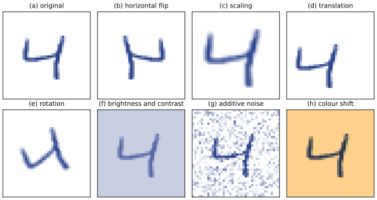
Why does augmentation help, and when does it produce invariant predictions? For a finite group there is a clean answer.
Result 9.2 (invariance by averaging; augmentation prefers invariant solutions) pp. 257–258
Let a finite group \(G\) act on the inputs, and for any function \(f\) define the group average \(\bar f(\bx)=\frac1{|G|}\sum_{g\in G}f(g\bx)\).
- \(\bar f\) is invariant, and \(\bar f=f\) whenever \(f\) is invariant.
- Let the augmented error be \(\wE(f)=\sum_n\frac1{|G|}\sum_{g}\ell(f(g\bx_n),t_n)\), every transformed copy keeping the target \(t_n\), with a loss \(\ell(y,t)\) convex in \(y\) (squared error, cross-entropy as a function of the logits, ...). Then \(\wE(\bar f)\le\wE(f)\).
So whenever the model class contains \(\bar f\) together with \(f\), the augmented problem has an invariant minimiser.
Proof
(1) For \(h\in G\), \[\bar f(h\bx)=\frac1{|G|}\sum_gf(g(h\bx))=\frac1{|G|}\sum_gf((g\circ h)\bx).\] The map \(g\mapsto g\circ h\) is a bijection of \(G\) (its inverse is \(g'\mapsto g'\circ h^{-1}\)), so the sum runs over all of \(G\) once and equals \(\sum_{g'}f(g'\bx)\): \(\bar f(h\bx)=\bar f(\bx)\). If \(f\) is invariant every term equals \(f(\bx)\).
(2) By (1), \(\bar f(g\bx_n)=\bar f(\bx_n)\) for all \(g\), so \[\wE(\bar f)=\sum_n\ell\Big(\frac1{|G|}\sum_gf(g\bx_n),t_n\Big)\le\sum_n\frac1{|G|}\sum_g\ell(f(g\bx_n),t_n)=\wE(f),\] by Jensen's inequality for the convex function \(\ell(\cdot,t_n)\) and the uniform weights \(1/|G|\) (Filling the gap 2.16). ∎
Remarks. For a continuous group (translations, rotations) the sums become averages over the group's invariant (Haar) measure and the same argument applies. A network class is generally not closed under group averaging, which is why augmentation only encourages, and an invariant architecture guarantees, invariance. Checked numerically for the four rotations of an image.
pp. 258–259 For transformations that change the input only a little, the effect of augmentation can be computed by a Taylor expansion (Bishop, 1995; Leen, 1995): it adds a penalty on the derivative of the output along the direction of the transformation, which is the tangent propagation regulariser; for additive noise the penalty is on all input derivatives (Exercise 9.2).
Filling the gap 9.2: augmentation with small transformations is tangent propagation; noise is Tikhonov regularisation pp. 258–259; Exercise 9.2
Let \(\bs(\bx,\xi)\) be a one-parameter transformation with \(\bs(\bx,0)=\bx\), tangent \(\btau=\partial\bs/\partial\xi\) and second derivative \(\bkappa=\partial^2\bs/\partial\xi^2\) at \(\xi=0\), and let \(\xi\) be random with \(\E[\xi]=0\), \(\E[\xi^2]=\sigma^2\), \(\E[\xi^3]=0\) and \(\E[\xi^4]=O(\sigma^4)\). For a scalar output \(y\) with gradient \(\nabla y\) and Hessian \(\nabla\nabla y\) with respect to the input, the expected squared error at one point is
\[ \E_\xi\big[(y(\bs(\bx,\xi))-t)^2\big]=(y-t)^2+\sigma^2\Big[(\btau^\T\nabla y)^2+(y-t)\big(\btau^\T\nabla\nabla y\,\btau+\nabla y^\T\bkappa\big)\Big]+O(\sigma^4). \]Derivation, the regularisers, and Exercise 9.2
Expansion. Put \(\phi(\xi)=y(\bs(\bx,\xi))\). By the chain rule \(\phi'(0)=\nabla y^\T\btau\) and \(\phi''(0)=\btau^\T\nabla\nabla y\,\btau+\nabla y^\T\bkappa\). For \(g(\xi)=(\phi(\xi)-t)^2\), \(g'=2(\phi-t)\phi'\) and \(g''=2\phi'^2+2(\phi-t)\phi''\). Taylor's theorem to fourth order, \[g(\xi)=g(0)+g'(0)\xi+\tfrac12g''(0)\xi^2+\tfrac16g'''(0)\xi^3+O(\xi^4),\] and the moment assumptions give \(\E g=g(0)+\tfrac12g''(0)\sigma^2+O(\sigma^4)\), which is the display. A numerical experiment rotates the input of a small tanh network by \(\xi\sim\N(0,\sigma^2)\) (so \(\btau=\bJ\bx\) with \(\bJ\) the \(90^\circ\) rotation and \(\bkappa=-\bx\)), computes the expectation by Gauss–Hermite quadrature, and finds that halving \(\sigma\) divides the error of the formula by 15.0, as an \(O(\sigma^4)\) remainder should.
Tangent propagation. Summing over the training set, \(\E[\wE]=E+\sigma^2\Omega+O(\sigma^4)\) with \(\Omega\) half the sum of the bracket. For a large data set, replace sums by integrals against \(p(\bx)p(t\given\bx)\). The term multiplying \((y-t)\) then integrates to \(\int(y(\bx)-\E[t\given\bx])(\cdots)p(\bx)\,\d\bx\). The minimiser of the regularised error is \(y=\E[t\given\bx]+O(\sigma^2)\) (the minimiser of the sum of squares is the conditional mean, Result 4.9), so this term contributes only \(O(\sigma^4)\) and, to leading order, \[ \Omega=\frac12\int(\btau^\T\nabla y)^2\,p(\bx)\,\d\bx, \] the tangent propagation regulariser of Simard et al. (1992): it penalises the rate of change of the output along the transformation. Several transformations, or a vector \(\bxi\) of uncorrelated parameters, add their terms.
Additive noise. For \(\bs(\bx,\bxi)=\bx+\bxi\) with \(\E[\bxi\bxi^\T]=\sigma^2\bI\), the same expansion in each coordinate gives \(\btau_i=\mathbf e_i\) and \(\bkappa=\bzero\), so the leading regulariser is \(\Omega=\frac12\int\|\nabla_{\bx}y\|^2p(\bx)\,\d\bx\): a Tikhonov penalty on the input gradient (checked numerically, same \(\sigma^4\) scaling).
Exercise 9.2 (linear model, exact). For \(y=w_0+\sum_iw_ix_i\) with independent noise \(\epsilon_{ni}\), \(\E[\epsilon_{ni}]=0\), \(\E[\epsilon_{ni}\epsilon_{nj}]=\delta_{ij}\sigma^2\), the noisy output is \(y_n+\sum_iw_i\epsilon_{ni}\), so \[ \E\Big[\tfrac12\sum_n\big(y_n+\textstyle\sum_iw_i\epsilon_{ni}-t_n\big)^2\Big]=E_D+\sum_n(y_n-t_n)\sum_iw_i\E[\epsilon_{ni}]+\tfrac12\sum_n\sum_{i,j}w_iw_j\E[\epsilon_{ni}\epsilon_{nj}]=E_D+\frac{N\sigma^2}2\sum_{i=1}^Dw_i^2 . \] This is weight decay with \(\lambda=N\sigma^2\) and the bias \(w_0\) excluded, exactly, with no Taylor remainder. Erratum (solutions manual). The manual's final line has \(\tfrac12\sigma^2\sum_iw_i^2\), dropping the factor \(N\) from the sum over data points; a Monte Carlo check (20 000 noise draws, \(N=25\)) gives an added term of 4.31 against \(N\sigma^2\|\bw\|^2/2=4.34\) and the manual's 0.17. ∎
9.1.4 Equivariance
pp. 259–260 Sometimes the output should not stay fixed but move with the input. For an image \(I\), a segmentation network \(S\) and a translation \(T\),
\[ S(T(I))=T(S(I)), \tag{9.2} \]more generally \(S(T(I))=\widetilde T(S(I))\) with a matching transformation \(\widetilde T\) of the output space (9.3) (a shift on a coarser grid, or a change of an angle when \(S\) measures orientation). Invariance is the special case where the output transformation is the identity:
\[ C(T(I))=C(I). \tag{9.4} \]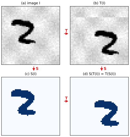
Result 9.3 (which maps are translation equivariant) pp. 259–260, (9.2)–(9.4)
Let images live on a cyclic grid of pixels \(\bm p\), and let \((T_{\bm a}I)[\bm p]=I[\bm p-\bm a]\). Then: (1) every pointwise map \(I\mapsto\varphi\circ I\) is equivariant; (2) every convolution \((K*I)[\bm p]=\sum_{\bm q}K[\bm q]\,I[\bm p-\bm q]\) is equivariant; (3) compositions of equivariant maps are equivariant; (4) the sum (or mean, or maximum) over all pixels is invariant. Hence a stack of convolutions and pointwise nonlinearities followed by global pooling is translation invariant, and without the pooling it is equivariant.
Proof
(1) \[(\varphi\circ T_{\bm a}I)[\bm p]=\varphi(I[\bm p-\bm a])=(T_{\bm a}(\varphi\circ I))[\bm p].\] (2) \[(K*T_{\bm a}I)[\bm p]=\sum_{\bm q}K[\bm q]I[\bm p-\bm q-\bm a]=(K*I)[\bm p-\bm a]=(T_{\bm a}(K*I))[\bm p].\] (3) If \(S_1T=TS_1\) and \(S_2T=TS_2\), then \(S_2S_1T=S_2TS_1=TS_2S_1\). (4) \(\sum_{\bm p}I[\bm p-\bm a]=\sum_{\bm p}I[\bm p]\) because \(\bm p\mapsto\bm p-\bm a\) is a bijection of the cyclic grid; the same holds for the maximum. The segmentation of Figure 9.2 is a box convolution followed by a pointwise threshold, so (1)–(3) give (9.2). On a finite non-cyclic grid the statements hold away from the borders. A subsampling layer that keeps every second pixel turns a shift by an even \(\bm a\) into a shift by \(\bm a/2\): an example of (9.3) with \(\widetilde T\neq T\). ∎
9.2 Weight Decay
See also the companion course, Section 3.1.4 (regularised least squares) and Section 3.5.3 (effective number of parameters); in this course, Result 4.7 (ridge regression) and Section 2.6.2 (the penalty as a Gaussian prior).
pp. 260–262 The penalty in (9.1) is the negative log of a zero-mean Gaussian prior on the weights (Section 2.6.2). It is a crude way to encode prior knowledge, which is usually about the function, not the weights. Its gradient is trivial to compute,
\[ \nabla\wE(\bw)=\nabla E(\bw)+\lambda\bw , \tag{9.5} \]and in a gradient step it shrinks every weight by a constant factor, hence the name weight decay.
Filling the gap 9.3: why "decay", in discrete and continuous time p. 260; Exercise 9.3
One gradient step on (9.1) with learning rate \(\rho\) is \(\bw\leftarrow(1-\rho\lambda)\bw-\rho\nabla E(\bw)\).
Derivation
Insert (9.5) into \(\bw^{(\tau+1)}=\bw^{(\tau)}-\rho\nabla\wE\). Where the data do not pull on a weight (\(\partial E/\partial w_i=0\)), it is multiplied by \(1-\rho\lambda\) at every step, so \(w_i^{(\tau)}=(1-\rho\lambda)^\tau w_i^{(0)}\to0\) geometrically when \(0<\rho\lambda<2\). In the limit of small steps, \(\bw(t)\) with \(t=\rho\tau\) obeys \(\d\bw/\d t=-\nabla E-\lambda\bw\); with \(E\) absent (Exercise 9.3, regulariser \(\Omega=\frac12\bw^\T\bw\), \(\lambda=1\)) this is \(\d\bw/\d t=-\bw\), solved by \(\bw(t)=e^{-t}\bw(0)\) (differentiate to verify; uniqueness from the linear ODE theory). Every component decays exponentially at the same rate (checked by an Euler integration). Erratum. Exercise 9.3 prints \(\Omega(\bw)=-\frac12\bw^\T\bw\), which would give \(\d\bw/\d t=+\bw\) and exponential growth, and writes \(\bw^{(\tau+1)}\) on both sides of (9.55); the manual silently uses \(+\frac12\bw^\T\bw\). ∎
Figure 9.3 shows the effect of the penalty on a quadratic error with axes along the Hessian's eigenvectors: the minimum moves towards the origin, much more along the direction in which the error is flat.
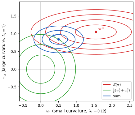
Result 9.4 (weight decay on a quadratic error; effective number of parameters) pp. 261–262, Figure 9.3
Let \(E(\bw)=E_0+\frac12(\bw-\bws)^\T\bH(\bw-\bws)\) with \(\bH=\sum_j\eta_j\bu_j\bu_j^\T\) positive semi-definite. The minimiser \(\widehat\bw\) of \(E+\frac\lambda2\bw^\T\bw\), \(\lambda>0\), has eigen-coordinates \[ \bu_j^\T\widehat\bw=\frac{\eta_j}{\eta_j+\lambda}\,\bu_j^\T\bws . \] Directions with \(\eta_j\gg\lambda\) are kept, those with \(\eta_j\ll\lambda\) are suppressed. The effective number of parameters \(\gamma(\lambda)=\sum_j\eta_j/(\eta_j+\lambda)\) decreases from the number of non-zero eigenvalues (at \(\lambda=0\)) to 0 (as \(\lambda\to\infty\)).
Proof
The regularised error is a quadratic with Hessian \(\bH+\lambda\bI\), positive definite, so its unique minimiser solves \((\bH+\lambda\bI)\widehat\bw=\bH\bws\). Multiplying by \(\bu_j^\T\) and using \(\bu_j^\T\bH=\eta_j\bu_j^\T\) gives \((\eta_j+\lambda)\bu_j^\T\widehat\bw=\eta_j\bu_j^\T\bws\). Each term of \(\gamma\) is decreasing in \(\lambda\), equal to 1 at \(\lambda=0\) when \(\eta_j>0\) and tending to 0. The quantity \(\gamma\) is the trace of \((\bH+\lambda\bI)^{-1}\bH\), the matrix that maps \(\bws\) to \(\widehat\bw\); for linear regression it is the degrees of freedom of the fit, and from the Bayesian side it is the \(\gamma\) of the evidence framework (companion Section 3.5.3). ∎
9.2.1 Consistent regularizers
See also the companion course, Section 5.5.1 and Result 5.12, which prove the same transformation rules for Bishop (2006).
pp. 262–264 Take a two-layer network with linear outputs,
\[ z_j=h\Big(\sum_iw_{ji}x_i+w_{j0}\Big), \tag{9.6} \] \[ y_k=\sum_jw_{kj}z_j+w_{k0}. \tag{9.7} \]If the inputs are linearly transformed, \(x_i\to\widetilde x_i=ax_i+b\) (9.8), the same mapping is obtained with \(\widetilde w_{ji}=w_{ji}/a\) (9.9) and \(\widetilde w_{j0}=w_{j0}-\frac ba\sum_iw_{ji}\) (9.10); if the outputs are transformed, \(y_k\to cy_k+d\) (9.11), it is enough to use \(\widetilde w_{kj}=cw_{kj}\) (9.12) and \(\widetilde w_{k0}=cw_{k0}+d\) (9.13). A regulariser should not prefer one of two equivalent networks over the other. Plain weight decay fails this test; a version that treats the layers separately and leaves out the biases passes it:
\[ \frac{\lambda_1}2\sum_{w\in\mathcal W_1}w^2+\frac{\lambda_2}2\sum_{w\in\mathcal W_2}w^2 . \tag{9.14} \]Result 9.5 (consistent regulariser, with the correct rescaling) pp. 262–263, (9.6)–(9.14); Exercise 9.4
- The transformations (9.9)–(9.10) leave the network function unchanged under (9.8), and (9.12)–(9.13) turn it into \(cy_k+d\).
- The value of (9.14) is unchanged if the coefficients are rescaled as \(\lambda_1\to a^2\lambda_1\) and \(\lambda_2\to c^{-2}\lambda_2\). Erratum: the book (like Bishop, 2006) prints \(a^{1/2}\) and \(c^{-1/2}\); with those exponents the value changes (checked: 13.66 becomes 2.75 for a random network with \(a=2.5\), \(c=0.3\)).
- If the data term is \(\frac\beta2\sum_n\|\by_n-\bt_n\|^2\) and the noise precision is rescaled with the targets, \(\beta\to\beta/c^2\), then the whole regularised objective is unchanged, so minimisers on the original and on the transformed data correspond exactly. With \(\beta\) held fixed the objective is multiplied by \(c^2\) in its data term only, and the rescaling that preserves minimisers is \(\lambda_1\to a^2c^2\lambda_1\), \(\lambda_2\to\lambda_2\).
Proof
(1) With (9.8)–(9.10), \[\sum_i\widetilde w_{ji}\widetilde x_i+\widetilde w_{j0}=\sum_i\frac{w_{ji}}a(ax_i+b)+w_{j0}-\frac ba\sum_iw_{ji}=\sum_iw_{ji}x_i+w_{j0},\] so every \(z_j\) is unchanged; with (9.12)–(9.13), \(\sum_jcw_{kj}z_j+cw_{k0}+d=cy_k+d\) (Exercise 9.4).
(2) Biases do not appear in (9.14), so the shifts in (9.10) and (9.13) do not matter. Under (9.9), \(\sum_{\mathcal W_1}\widetilde w^2=a^{-2}\sum_{\mathcal W_1}w^2\); under (9.12), \(\sum_{\mathcal W_2}\widetilde w^2=c^2\sum_{\mathcal W_2}w^2\). The value is unchanged iff \(\widetilde\lambda_1a^{-2}=\lambda_1\) and \(\widetilde\lambda_2c^2=\lambda_2\).
(3) The residuals transform as \(\widetilde y-\widetilde t=c(y-t)\), so the data term becomes \(\frac{\widetilde\beta}2c^2\sum\|\by-\bt\|^2\), equal to the original if \(\widetilde\beta=\beta/c^2\); with (2) the full objective is then the same function of the original weights, and the transformation of the weights is a bijection, so minimisers map to minimisers. If \(\beta\) is fixed, the objective becomes \(c^2\times\)(data term) \(+\) regulariser, which is \(c^2\) times the original objective iff each regulariser coefficient carries an extra \(c^2\). ∎
The regulariser (9.14) is the negative log of the prior
\[ p(\bw\given\alpha_1,\alpha_2)\propto\exp\Big(-\frac{\alpha_1}2\sum_{w\in\mathcal W_1}w^2-\frac{\alpha_2}2\sum_{w\in\mathcal W_2}w^2\Big), \tag{9.15} \]which is improper (it cannot be normalised, because the biases are unconstrained). In practice the biases get their own Gaussian priors, giving four hyperparameters \(\alpha_1^w,\alpha_1^b,\alpha_2^w,\alpha_2^b\), whose effect is shown in Figure 9.4. More generally the weights can be split into any groups \(\mathcal W_k\),
\[ \Omega(\bw)=\frac12\sum_k\alpha_k\|\bw\|_k^2, \tag{9.16} \] \[ \|\bw\|_k^2=\sum_{j\in\mathcal W_k}w_j^2 , \tag{9.17} \]for example one group per layer (or, with one group per input and \(\alpha_k\) learned, automatic relevance determination).
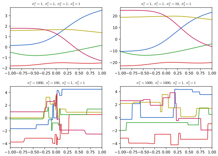
Filling the gap 9.4: what the four hyperparameters do p. 263, Figure 9.4
The book describes the effects qualitatively. Write \(\sigma\) for prior standard deviations and \(f(x)=\sum_{j=1}^Mv_j\tanh(w_jx+b_j)+c\).
Derivation
Vertical scale. Given the first layer, \(\var[f(x)]=\sigma_{2w}^2\sum_j\tanh^2(w_jx+b_j)+\sigma_{2b}^2\), so the size of the variations is proportional to \(\sigma_{2w}\) (at most \(\sqrt M\sigma_{2w}\)) and \(\sigma_{2b}\) sets the range of vertical offsets. Multiplying \(\sigma_{2w}\) by 10 multiplies every sampled function's variation by exactly 10 for the same random numbers (checked).
Horizontal scale. Unit \(j\) changes from \(-1\) to \(+1\) around \(x_j=-b_j/w_j\), over a width of order \(1/|w_j|\sim1/\sigma_{1w}\): large first-layer weights make step-like units.
Horizontal range. \(x_j=-b_j/w_j\) is a ratio of independent zero-mean Gaussians. Writing \(b_j=\sigma_{1b}u\), \(w_j=\sigma_{1w}v\) with \(u,v\) standard normal, \(x_j=-(\sigma_{1b}/\sigma_{1w})(u/v)\). The point \((v,u)\) has a rotation-invariant density, so its angle \(\theta\) is uniform and \(u/v=\tan\theta\) has the standard Cauchy density \(1/(\pi(1+s^2))\). Hence the switch points are Cauchy with scale \(\sigma_{1b}/\sigma_{1w}\): 0.1 in the bottom-left panel (steps near the origin) and 1 in the bottom-right one (steps across \([-1,1]\)), as plotted.
Labels. With precisions, \(\sigma=\alpha^{-1/2}\): \(\alpha_1^w=1000\) would mean \(\sigma_{1w}\approx0.03\) and almost linear functions, not steps, and \(\alpha_2^w=10\) would shrink the top-right panel. Both contradict the plots, so the numbers in the panel titles are standard deviations; as precisions they would read \(1,10^{-2},10^{-6},10^{-4}\). The companion course flags the same erratum in Bishop (2006), Figure 5.11. ∎
9.2.2 Generalized weight decay
See also the companion course, Result 3.6 (penalised and constrained least squares are equivalent) and Filling the gap 3.3 (why the lasso gives sparse solutions).
pp. 264–266 A family of penalties generalises (9.1):
\[ \Omega(\bw)=\frac\lambda2\sum_{j=1}^M|w_j|^q , \tag{9.18} \]with \(q=2\) the quadratic regulariser and \(q=1\) the lasso (Tibshirani, 1996), which for large enough \(\lambda\) sets some weights exactly to zero: a sparse model. Minimising
\[ E(\bw)+\frac\lambda2\sum_{j=1}^M|w_j|^q \tag{9.19} \]is equivalent to minimising \(E(\bw)\) subject to
\[ \sum_{j=1}^M|w_j|^q\le\eta \tag{9.20} \]for a suitable \(\eta\) (Exercise 9.5), and the shape of the constraint region explains the sparsity (Figures 9.5, 9.6).
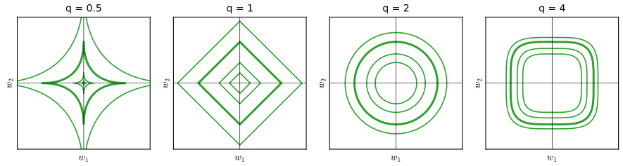
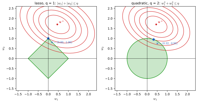
lq_constrained_2d). Reproduces Bishop and Bishop (2024), Figure 9.6. Download: PDF · SVGResult 9.6 (penalised and constrained problems) p. 265; Exercise 9.5
- For any \(E\) and any \(q>0\): if \(\widehat\bw\) minimises (9.19), then it minimises \(E\) subject to (9.20) with \(\eta=\sum_j|\widehat w_j|^q\).
- If \(E\) is convex, \(q\ge1\) and \(\eta>0\), every minimiser of the constrained problem minimises (9.19) for some \(\lambda\ge0\) (half the Lagrange multiplier of the constraint, as in Appendix C of the book).
- Along the solution path, \(\eta(\lambda)=\sum_j|\widehat w_j(\lambda)|^q\) is non-increasing and \(E(\widehat\bw(\lambda))\) non-decreasing in \(\lambda\).
Proof
Write \(P(\bw)=\sum_j|w_j|^q\). (1) If \(P(\bw)\le\eta=P(\widehat\bw)\), optimality of \(\widehat\bw\) for (9.19) gives \(E(\bw)+\frac\lambda2P(\bw)\ge E(\widehat\bw)+\frac\lambda2\eta\), hence \(E(\bw)\ge E(\widehat\bw)+\frac\lambda2(\eta-P(\bw))\ge E(\widehat\bw)\). No convexity is needed.
(2) With \(E\) and \(P\) convex and \(P(\bzero)=0<\eta\) (Slater's condition), convex duality guarantees a multiplier \(\mu\ge0\) such that a constrained minimiser \(\bw^\circ\) minimises the Lagrangian \(E(\bw)+\mu(P(\bw)-\eta)\) and \(\mu(P(\bw^\circ)-\eta)=0\) (complementary slackness). Dropping the constant \(-\mu\eta\), \(\bw^\circ\) minimises (9.19) with \(\lambda=2\mu\). If the constraint is inactive, \(\mu=0\) and \(\bw^\circ\) is an unconstrained minimiser. For \(q<1\) or non-convex \(E\), part (2) can fail: some constrained solutions are reached by no \(\lambda\).
(3) Let \(\lambda_1<\lambda_2\) with minimisers \(\bw_1,\bw_2\) and \(P_i=P(\bw_i)\), \(E_i=E(\bw_i)\). Optimality of each for its own \(\lambda\): \(E_1+\frac{\lambda_1}2P_1\le E_2+\frac{\lambda_1}2P_2\) and \(E_2+\frac{\lambda_2}2P_2\le E_1+\frac{\lambda_2}2P_1\). Adding, \(\frac{\lambda_2-\lambda_1}2(P_2-P_1)\le0\), so \(P_2\le P_1\); then the first inequality gives \(E_1\le E_2+\frac{\lambda_1}2(P_2-P_1)\le E_2\). The precise map \(\lambda\mapsto\eta\) depends on \(E\) (checked on the demo's data: \(\eta\) falls from 6.87 to 0.02 as \(\lambda\) goes from 5 to 290). ∎
Filling the gap 9.5: why the lasso gives exact zeros and \(q>1\) never does pp. 264–266
The figure argument (the error contours touch the diamond at a corner) can be turned into conditions that hold for an open set of problems.
Derivation
Optimality for \(q=1\). For convex differentiable \(E\), \(\widehat\bw\) minimises \(E+\frac\lambda2\sum_j|w_j|\) iff \(\bzero\) lies in the subdifferential, i.e. for each \(j\): \[ \frac{\partial E}{\partial w_j}+\frac\lambda2\sign(\widehat w_j)=0\ \ (\widehat w_j\ne0),\qquad\Big|\frac{\partial E}{\partial w_j}\Big|\le\frac\lambda2\ \ (\widehat w_j=0). \] The second condition is an inequality: it keeps holding when the data are perturbed a little, so exact zeros are stable. For least squares, \(E=\frac12\|\bt-\bX\bw\|^2\), the condition reads \(|\mathbf x_j^\T\mathbf r|\le\lambda/2\) with residual \(\mathbf r=\bt-\bX\widehat\bw\) (checked on the demo's solution), and \(\widehat\bw=\bzero\) iff \(\lambda\ge\lambda_{\max}=2\max_j|\mathbf x_j^\T\bt|\).
\(q>1\). The penalty is differentiable with derivative \(\frac{\lambda q}2|w|^{q-1}\sign(w)\), which vanishes at 0. So \(\widehat w_j=0\) requires \(\partial E/\partial w_j=0\) exactly at \(\widehat\bw\): an equation, not an inequality, satisfied only for exceptional data. The quadratic penalty shrinks but does not select.
Orthonormal inputs. If \(\bX^\T\bX=\bI\), then \(E=\frac12\|\bw-\bw_{\rm LS}\|^2+\const\) with \(\bw_{\rm LS}=\bX^\T\bt\), and the problem separates. Ridge gives \(\widehat w_j=w_{{\rm LS},j}/(1+\lambda)\); the lasso gives the soft threshold \(\widehat w_j=\sign(w_{{\rm LS},j})\max(|w_{{\rm LS},j}|-\lambda/2,0)\) (minimise \(\frac12(w-c)^2+\frac\lambda2|w|\) separately for \(w>0\), \(w<0\) and compare with \(w=0\)). For general \(\bX\) each coordinate subproblem has this form, which is the cyclic coordinate descent used by the demo: \(w_j\leftarrow\mathrm{soft}(\mathbf x_j^\T\mathbf r+\|\mathbf x_j\|^2w_j,\lambda/2)/\|\mathbf x_j\|^2\).
Convexity. For \(q\ge1\), \(|w|^q\) is convex, so the sum and its sublevel sets are convex. For \(q<1\) the midpoint of \((1,0)\) and \((0,1)\) has \(2\cdot2^{-q}=2^{1-q}>1\), so the region is not convex: \(q<1\) still selects variables (the corners are even sharper) but the optimisation may have local minima. ∎
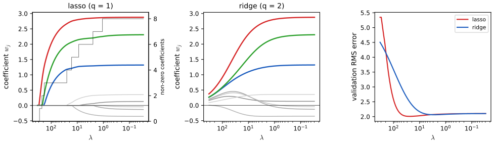
Regularisation moves the problem of choosing the model size into choosing \(\lambda\), which is the subject of the next section.
9.3 Learning Curves
p. 266 Model size, data-set size and \(\lambda\) all trade bias against variance; so does the training process. Learning curves plot the training and validation error against the iteration number during training.
9.3.1 Early stopping
See also the companion course, Section 5.5.2 and Result 5.13 (the same eigen-analysis), and its early-stopping demo; in this course, gradient descent on a quadratic: Result 7.6.
pp. 266–267 The training error usually falls steadily, while the error on held-out (validation) data falls and then rises as the network starts to over-fit. Stopping at the minimum of the validation error is early stopping (Figure 9.7). Informally the effective number of parameters starts small and grows during training.
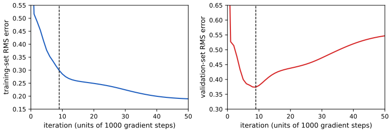
pp. 267–268 For a quadratic error the link with weight decay can be made precise (Bishop, 1995a). With axes along the Hessian's eigenvectors, gradient descent from the origin first moves along the steep direction and only later along the flat one (Figure 9.8), so stopping early leaves the flat directions suppressed, as weight decay does (compare Figure 9.3). Quantitatively, \(\rho\tau\) (learning rate times number of steps) plays the role of \(1/\lambda\) (Exercise 9.6). (The book's text writes \(\tau\eta\) with \(\eta\) the learning rate, while Exercise 9.6 calls the learning rate \(\rho\) and the eigenvalues \(\eta_j\); these notes follow the exercise.)
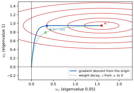
Result 9.7 (early stopping is weight decay, up to a factor of 2) pp. 267–268; Exercise 9.6, (9.56)–(9.61)
Let \(E=E_0+\frac12(\bw-\bws)^\T\bH(\bw-\bws)\) (9.56) with \(\bH\) constant and positive definite, \(\bH\bu_j=\eta_j\bu_j\) (9.59), and run gradient descent \(\bw^{(\tau)}=\bw^{(\tau-1)}-\rho\nabla E\) (9.57) from \(\bw^{(0)}=\bzero\).
- The components \(w_j=\bw^\T\bu_j\) satisfy \[ w_j^{(\tau)}=\{1-(1-\rho\eta_j)^\tau\}\,w_j^\star , \tag{9.58} \] and \(\bw^{(\tau)}\to\bws\) iff \(|1-\rho\eta_j|<1\) for all \(j\).
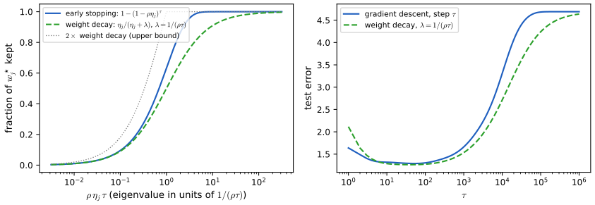
- (Sandwich.) If \(0<\rho\eta_j\le1\) for all \(j\) and \(\lambda=1/(\rho\tau)\), then for every \(j\) and every \(\tau\ge1\) \[ \frac{\eta_j}{\eta_j+\lambda}\ \le\ 1-(1-\rho\eta_j)^\tau\ \le\ \frac{2\eta_j}{\eta_j+\lambda}. \] So early stopping after \(\tau\) steps and weight decay with \(\lambda=1/(\rho\tau)\) keep the same fraction of every eigen-direction up to a factor of 2.
- In particular \(w_j^{(\tau)}\simeq w_j^\star\) when \(\eta_j\gg(\rho\tau)^{-1}\) (9.60) and \(|w_j^{(\tau)}|\simeq\rho\tau\eta_j|w_j^\star|\ll|w_j^\star|\) when \(\eta_j\ll(\rho\tau)^{-1}\) (9.61).
- The effective number of parameters of early stopping, \(\gamma(\tau)=\sum_j\{1-(1-\rho\eta_j)^\tau\}\), increases with \(\tau\) and lies between \(\gamma_{\rm WD}(1/\rho\tau)\) and \(2\gamma_{\rm WD}(1/\rho\tau)\), with \(\gamma_{\rm WD}\) the weight-decay count of Result 9.4.
Proof
(1) \(\nabla E=\bH(\bw-\bws)\), so \[w_j^{(\tau)}-w_j^\star=\bu_j^\T(\bw^{(\tau-1)}-\bws)-\rho\bu_j^\T\bH(\bw^{(\tau-1)}-\bws)=(1-\rho\eta_j)(w_j^{(\tau-1)}-w_j^\star).\] Iterating from \(w_j^{(0)}-w_j^\star=-w_j^\star\) gives \(w_j^{(\tau)}-w_j^\star=-(1-\rho\eta_j)^\tau w_j^\star\), which is (9.58). The factor tends to 0 iff \(|1-\rho\eta_j|<1\).
(2) Put \(a=\rho\eta_j\in(0,1]\) and \(x=a\tau=\eta_j/\lambda\), so the weight-decay fraction is \(r=x/(1+x)\) and the early-stopping fraction is \(g=1-(1-a)^\tau\). Lower bound: \(0\le1-a\le e^{-a}\), so \((1-a)^\tau\le e^{-x}\) and \(g\ge1-e^{-x}\); since \(e^x\ge1+x\), \(e^{-x}\le1/(1+x)\) and \(1-e^{-x}\ge x/(1+x)=r\). Upper bound: Bernoulli's inequality \((1-a)^\tau\ge1-\tau a\) (for \(a\le1\) and integer \(\tau\ge1\), by induction: \((1-a)^{\tau+1}\ge(1-\tau a)(1-a)\ge1-(\tau+1)a\)) gives \(g\le x\); also \(g\le1\). If \(x\le1\), \(x\le2x/(1+x)\) because \(1+x\le2\); if \(x\ge1\), \(1\le2x/(1+x)\) because \(1+x\le2x\). So \(g\le\min(1,x)\le2r\).
(3) If \(x\gg1\), \(g\ge x/(1+x)\approx1\). If \(x\ll1\), \(r\le g\le x\) with \(r=x/(1+x)\approx x\), so \(g\approx x=\rho\tau\eta_j\).
(4) Each term of \(\gamma(\tau)\) increases with \(\tau\) because \(0\le1-\rho\eta_j<1\); summing (2) over \(j\) gives the bounds. ∎
The same holds in continuous time (gradient flow \(\d\bw/\d t=-\nabla E\)), where \(g=1-e^{-\eta_jt}\) and \[x/(1+x)\le1-e^{-x}\le\min(1,x)\le2x/(1+x).\] Both bounds are checked on a grid of \(\rho\eta_j\) and \(\tau\); Figure 9.S2 (left) shows the two filters. If \(1<\rho\eta_j<2\), descent still converges but the steep directions overshoot and oscillate, and the lower bound can fail at odd \(\tau\).
Filling the gap 9.6: why the validation curve is U-shaped (linear regression, exactly) pp. 266–267
For a linear model the bias and variance along the gradient-descent path can be written down.
Derivation
Let \(\bt=\bX\bth+\bep\) with fixed \(\bX\) (full column rank), \(\E\bep=\bzero\), \(\cov\bep=\sigma^2\bI\), and \(E=\frac12\|\bt-\bX\bw\|^2\), so \(\bH=\bX^\T\bX=\sum_j\eta_j\bu_j\bu_j^\T\) and \(\bws=\bw_{\rm LS}=\bH^{-1}\bX^\T\bt=\bth+\bH^{-1}\bX^\T\bep\). By (9.58), \(\bu_j^\T\bw^{(\tau)}=g_j\bu_j^\T\bw_{\rm LS}\) with \(g_j=1-(1-\rho\eta_j)^\tau\). The coordinate \(\bu_j^\T\bH^{-1}\bX^\T\bep=\eta_j^{-1}\bu_j^\T\bX^\T\bep\) has mean 0 and variance \(\eta_j^{-2}\sigma^2\bu_j^\T\bX^\T\bX\bu_j=\sigma^2/\eta_j\), so \[ \E\,\|\bw^{(\tau)}-\bth\|^2=\sum_j\Big[(1-g_j)^2(\bu_j^\T\bth)^2+g_j^2\frac{\sigma^2}{\eta_j}\Big]. \] As \(\tau\) grows, every \(g_j\) increases from 0 to 1: the bias terms fall and the variance terms rise, the variance most in the directions with small \(\eta_j\), which are learned last. The sum is therefore typically U-shaped in \(\tau\), and the same expression with \(g_j=\eta_j/(\eta_j+\lambda)\) gives the U-shape in \(1/\lambda\). Figure 9.S2 (right) computes both for a linear model with 20 inputs whose scales range over two orders of magnitude: the two test-error curves nearly coincide when plotted against \(\tau\) and \(1/(\rho\tau)\). ∎
9.3.2 Double descent
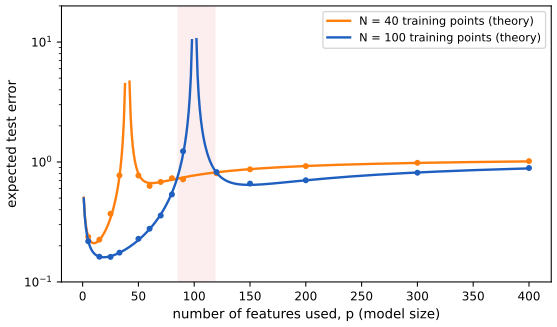
pp. 268–270 Classical bias–variance reasoning says the number of parameters must be limited to the size of the data set. Yet modern networks generalise well with far more parameters than needed to fit the training data exactly (Zhang et al., 2016), sometimes trained to zero training error. The two views are reconciled by double descent (Belkin et al., 2019): as model complexity grows, the test error first follows the classical U-shape, peaks near the interpolation threshold (the smallest model that can fit the training data exactly), and then decreases again (Figure 9.9). Nakkiran et al. (2019) define the effective model complexity as the largest training set a model can fit to zero error; the peak occurs when it equals the actual number of training points. The same phenomenon appears against the number of epochs (Figure 9.10) and against \(1/\lambda\) (Yilmaz and Heckel, 2022), and it implies that more data can hurt (Figure 9.11).
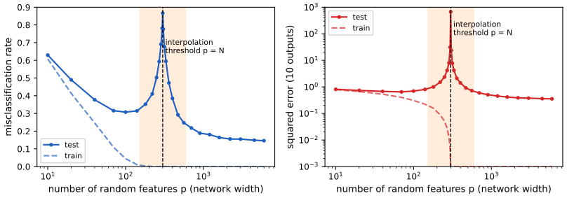
Two facts explain this figure. First, which interpolant is found: when \(p>N\), infinitely many weight vectors fit the data, and gradient descent from zero picks a particular one.
Filling the gap 9.7: the implicit bias of gradient descent: the minimum-norm interpolant pp. 268–269
"It seems to be a property of stochastic gradient descent that the implicit biases it introduces lead to good generalization." For least squares the implicit bias is exact.
Derivation
Let \(\bX\in\R^{N\times p}\) have rank \(N<p\) and \(E=\frac12\|\bX\bw-\bt\|^2\). Every gradient \(\bX^\T(\bX\bw-\bt)\) lies in the row space \(\mathcal R\) of \(\bX\), so gradient descent from \(\bw^{(0)}=\bzero\) stays in \(\mathcal R\). With \(0<\rho<2/\sigma_{\max}^2(\bX)\) the residual contracts in every direction of \(\mathcal R\) (the eigenvalue argument of Result 9.7 applied to \(\bX\bX^\T\), all of whose eigenvalues are positive), so the iterates converge to an interpolant in \(\mathcal R\). Any interpolant is \(\bw=\bX^+\bt+\mathbf n\) with \(\mathbf n\) in the null space of \(\bX\), which is orthogonal to \(\mathcal R\); hence \(\|\bw\|^2=\|\bX^+\bt\|^2+\|\mathbf n\|^2\), and the only interpolant in \(\mathcal R\) is the minimum-norm one \(\bX^+\bt=\bX^\T(\bX\bX^\T)^{-1}\bt\). Ridge regression gives the same limit: \[(\bX^\T\bX+\lambda\bI)^{-1}\bX^\T\bt=\bX^\T(\bX\bX^\T+\lambda\bI)^{-1}\bt\to\bX^+\bt\] as \(\lambda\to0\) (the push-through identity \[(\bX^\T\bX+\lambda\bI)\bX^\T=\bX^\T(\bX\bX^\T+\lambda\bI)\]). Both limits are checked numerically. So "train to zero error from a small initialisation" means "choose the smallest weights that fit". ∎
Second, how good that interpolant is. For a Gaussian design the test error of least squares and of minimum-norm interpolation is known exactly, and it shows the whole double-descent curve.
Result 9.8 (exact double descent for least squares with Gaussian inputs) pp. 268–270
Let \(\bx\sim\N(\bzero,\bI_D)\), \(t=\bx^\T\bbeta+\epsilon\) with \(\epsilon\sim\N(0,\sigma^2)\), and fit the first \(p\) coordinates by \(\widehat\bw=\bX_p^+\bt\) on \(N\) training points (least squares if \(p<N\), minimum-norm interpolation if \(p>N\)). Let \(\bbeta_p\) be the first \(p\) coefficients, \(\bbeta_{\bar p}\) the rest, and \(s^2=\sigma^2+\|\bbeta_{\bar p}\|^2\). The expected test error \(\mathcal E=\E[(t-\bx_p^\T\widehat\bw)^2]\) is (Belkin, Hsu and Xu, 2020) \[ \mathcal E=\begin{cases} s^2\Big(1+\dfrac p{N-p-1}\Big), & p\le N-2,\\[2mm] \|\bbeta_p\|^2\Big(1-\dfrac Np\Big)+s^2\Big(1+\dfrac N{p-N-1}\Big), & p\ge N+2, \end{cases} \] and it is infinite for \(N-1\le p\le N+1\).
Proof
Omitted features are noise. \(t=\bx_p^\T\bbeta_p+\nu\) with \(\nu=\bx_{\bar p}^\T\bbeta_{\bar p}+\epsilon\). Since the coordinates of \(\bx\) are independent, \(\nu\) is independent of \(\bx_p\), Gaussian with mean 0 and variance \(s^2\).
Test error. For a new pair, \(t-\bx_p^\T\widehat\bw=\nu+\bx_p^\T(\bbeta_p-\widehat\bw)\) with \((\bx_p,\nu)\) independent of the training set and \(\E[\bx_p\bx_p^\T]=\bI\), so \(\mathcal E=s^2+\E\|\widehat\bw-\bbeta_p\|^2\).
\(p\le N-2\). \(\bX_p\) has full column rank with probability 1 and \(\widehat\bw-\bbeta_p=(\bX_p^\T\bX_p)^{-1}\bX_p^\T\boldsymbol\nu\). Conditioning on \(\bX_p\), \(\E\|\cdot\|^2=s^2\Tr(\bX_p^\T\bX_p)^{-1}\). The matrix \(\bX_p^\T\bX_p\) is Wishart with \(N\) degrees of freedom and identity scale, whose inverse has mean \(\bI/(N-p-1)\) (a standard fact, e.g. Mardia, Kent and Bibby, 1979; checked by Monte Carlo), so \(\E\|\widehat\bw-\bbeta_p\|^2=s^2p/(N-p-1)\).
\(p\ge N+2\). Now \(\bX_p\) has full row rank and \[\widehat\bw=\bX_p^+(\bX_p\bbeta_p+\boldsymbol\nu)=\bP\bbeta_p+\bX_p^+\boldsymbol\nu,\] with \(\bP=\bX_p^+\bX_p\) the orthogonal projection onto the row space. So \(\widehat\bw-\bbeta_p=-(\bI-\bP)\bbeta_p+\bX_p^+\boldsymbol\nu\), and the cross term has mean zero. The rows of \(\bX_p\) are rotation invariant in distribution, so the row space is a uniformly random \(N\)-dimensional subspace and \(\E\bP=(N/p)\bI\) (its trace is \(N\) and it commutes with every rotation); hence \[\E\|(\bI-\bP)\bbeta_p\|^2=\bbeta_p^\T(\bI-\E\bP)\bbeta_p=\|\bbeta_p\|^2(1-N/p).\] Also \[\E\|\bX_p^+\boldsymbol\nu\|^2=s^2\E\Tr(\bX_p\bX_p^\T)^{-1}=s^2N/(p-N-1),\] now with the \(N\times N\) Wishart matrix \(\bX_p\bX_p^\T\) of \(p\) degrees of freedom.
Near \(p=N\). The smallest singular value of a nearly square Gaussian matrix is close to 0 with appreciable probability, and the inverse-Wishart mean is infinite when \(|N-p|\le1\). ∎
Reading the formula. Below the threshold the fit is unbiased in the included coordinates and the variance factor \(p/(N-p-1)\) explodes as \(p\to N\). Above it, the bias term \(\|\bbeta_p\|^2(1-N/p)\) is the part of the signal outside the row space, and the variance factor \(N/(p-N-1)\) decreases as \(p\) grows: more features spread the noise over more directions and the minimum-norm solution damps it. If the signal is spread over many features (as in Figure 9.11, \(\beta_j\propto1/j\)), the second descent can go below the first. The formula agrees with Monte Carlo below and above the threshold (checked to 3%).
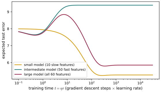
Filling the gap 9.8: why double descent appears in training time pp. 269–270
The book reports epoch-wise double descent without a mechanism. In a linear model it follows from the filters of Result 9.7.
Derivation (in the large-sample approximation)
By Filling the gap 9.6, in the eigenbasis of the input covariance the error along gradient flow is a sum over directions of a bias term \((1-g_j(t))^2(\cdots)\) and a variance term \(g_j(t)^2(\cdots)\), with \(g_j(t)=1-e^{-\eta_jt}\). When \(N\) is large the sample eigenvalues are close to the population ones, and each direction's contribution is a function of \(\eta_jt\) only: it changes around the time \(t\approx1/\eta_j\). A group of directions with similar eigenvalues therefore contributes a curve with a single transition time: a decrease if it carries more signal than noise, a U-shape or an increase if it carries mostly noise. With two well-separated groups (eigenvalues 1 and 0.01 in Figure 9.10), the total error is the sum of two such curves, shifted by a factor of 100 in time. If the fast group's variance outweighs its signal, the sum falls (fast signal learned), rises (fast group fits the noise), then falls again (slow signal learned): two descents. Without separated time scales, as for the small model, there is a single transition. Large networks contain features learned at very different speeds (different layers, different scales of the weights), which makes the same superposition plausible there (Heckel and Yilmaz, 2021). ∎
9.4 Parameter Sharing
See also the companion course, Section 5.5.6 (convolutional networks) and Result 5.16.
pp. 270–271 A hard alternative to penalties is to force groups of weights to be equal, learning one value per group (weight sharing, parameter tying). It reduces the degrees of freedom below the number of connections and usually encodes a known invariance; convolutional networks (Chapter 10) are the main example. It applies only when the constraints can be specified in advance.
Filling the gap 9.9: gradients for shared weights p. 271; Exercise 9.7
The gradient with respect to a shared parameter is the sum of the gradients of all the connections that use it.
Derivation
Let the connection weights be \(w_i=v_{k(i)}\), where \(k(i)\) is the group of connection \(i\) and \(v_k\) the free parameters, and let \(E(\bw)\) be the error as a function of all connection weights. By the chain rule, with \(\partial w_i/\partial v_k=1\) if \(k(i)=k\) and 0 otherwise, \[ \frac{\partial E}{\partial v_k}=\sum_i\frac{\partial E}{\partial w_i}\frac{\partial w_i}{\partial v_k}=\sum_{i:\,k(i)=k}\frac{\partial E}{\partial w_i}. \] So backpropagation is run unchanged, as if every connection had its own weight, and the derivatives of each group are added. Updating \(v_k\) (equivalently, giving every member of the group the same summed update) keeps the members equal if they start equal. The cost is that of ordinary backpropagation plus one addition per connection; automatic differentiation does this automatically when the same tensor is used in several places (checked with autograd for a layer whose \(2\times4\) weight matrix has three free parameters). ∎
9.4.1 Soft weight sharing
See also the companion course, Section 5.5.7 and Result 5.17; mixtures of Gaussians in this course: Section 3.2.9.
pp. 271–273 Nowlan and Hinton (1992) replace equality constraints by a penalty that encourages groups of similar weights, with the groups, their centres and spreads learned. Weight decay is a single zero-mean Gaussian prior; soft weight sharing uses a mixture of Gaussians (Section 3.2.9):
\[ p(\bw)=\prod_i\Big\{\sum_{j=1}^K\pi_j\N(w_i\given\mu_j,\sigma_j^2)\Big\}, \tag{9.21} \] \[ \Omega(\bw)=-\sum_i\ln\Big(\sum_{j=1}^K\pi_j\N(w_i\given\mu_j,\sigma_j^2)\Big), \tag{9.22} \] \[ \wE(\bw)=E(\bw)+\lambda\Omega(\bw), \tag{9.23} \]minimised jointly over the weights and the mixture parameters. With the responsibilities
\[ \gamma_j(w_i)=\frac{\pi_j\N(w_i\given\mu_j,\sigma_j^2)}{\sum_k\pi_k\N(w_i\given\mu_k,\sigma_k^2)}, \tag{9.24} \]and the unconstrained parametrisations \(\sigma_j^2=\exp(\xi_j)\) (9.27) and \(\pi_j=\exp(\eta_j)/\sum_{k=1}^K\exp(\eta_k)\) (9.30) (which enforce \(\sum_j\pi_j=1\), \(0\le\pi_j\le1\) (9.29)), the derivatives are as follows.
Result 9.9 (derivatives of the soft weight-sharing error) pp. 272–273, (9.24)–(9.31); Exercises 9.8–9.12
\[ \frac{\partial\wE}{\partial w_i}=\frac{\partial E}{\partial w_i}+\lambda\sum_j\gamma_j(w_i)\frac{w_i-\mu_j}{\sigma_j^2}, \tag{9.25} \] \[ \frac{\partial\wE}{\partial\mu_j}=\lambda\sum_i\gamma_j(w_i)\frac{\mu_j-w_i}{\sigma_j^2}, \tag{9.26} \] \[ \frac{\partial\wE}{\partial\xi_j}=\frac\lambda2\sum_i\gamma_j(w_i)\Big(1-\frac{(w_i-\mu_j)^2}{\sigma_j^2}\Big), \tag{9.28} \] \[ \frac{\partial\wE}{\partial\eta_j}=\lambda\sum_i\{\pi_j-\gamma_j(w_i)\}. \tag{9.31} \](The book's (9.28) omits the subscript \(j\) on \(\xi\).) Each derivative vanishes, with the responsibilities held fixed, when \(\mu_j\) is the responsibility-weighted mean of the weights, \(\sigma_j^2\) their responsibility-weighted variance about \(\mu_j\), and \(\pi_j\) the average responsibility: the M-step of the EM algorithm for a mixture of Gaussians fitted to the weights.
Proof
Write \(\N_{ij}=\N(w_i\given\mu_j,\sigma_j^2)\) and \(Z_i=\sum_k\pi_k\N_{ik}\), so \(\Omega=-\sum_i\ln Z_i\) and \(\gamma_j(w_i)=\pi_j\N_{ij}/Z_i\) (Bayes' theorem with prior \(p(j)=\pi_j\) and likelihood \(p(w\given j)=\N_{ij}\): Exercise 9.8). Differentiating \(\ln\N=-\frac12\ln(2\pi\sigma^2)-(w-\mu)^2/(2\sigma^2)\): \[ \frac{\partial\N}{\partial w}=-\N\frac{w-\mu}{\sigma^2},\qquad\frac{\partial\N}{\partial\mu}=\N\frac{w-\mu}{\sigma^2},\qquad\frac{\partial\N}{\partial\sigma^2}=\N\Big(-\frac1{2\sigma^2}+\frac{(w-\mu)^2}{2\sigma^4}\Big). \] (9.25). \[\partial\Omega/\partial w_i=-\frac1{Z_i}\sum_j\pi_j\partial\N_{ij}/\partial w_i=\sum_j\gamma_j(w_i)(w_i-\mu_j)/\sigma_j^2\] (Exercise 9.9). (9.26). \(\mu_j\) appears in every \(Z_i\): \[\partial\Omega/\partial\mu_j=-\sum_i\frac{\pi_j}{Z_i}\N_{ij}\frac{w_i-\mu_j}{\sigma_j^2}=\sum_i\gamma_j(w_i)\frac{\mu_j-w_i}{\sigma_j^2}\] (Exercise 9.10). (9.28). \(\partial\sigma_j^2/\partial\xi_j=\sigma_j^2\), so \[\partial\N_{ij}/\partial\xi_j=\N_{ij}\big(-\frac12+\frac{(w_i-\mu_j)^2}{2\sigma_j^2}\big)\] and \[\partial\Omega/\partial\xi_j=\frac12\sum_i\gamma_j(w_i)\big(1-(w_i-\mu_j)^2/\sigma_j^2\big)\] (Exercise 9.11; the manual differentiates with respect to \(\sigma_j\) and leaves out the chain-rule factor \(\partial\sigma_j/\partial\xi_j=\sigma_j/2\) that turns its result into (9.28)). (9.31). For the softmax, \(\partial\pi_k/\partial\eta_j=\delta_{jk}\pi_j-\pi_j\pi_k\) (9.63) (differentiate \(e^{\eta_k}/\sum_le^{\eta_l}\) by the quotient rule). Then \[\partial\Omega/\partial\eta_j=-\sum_i\frac1{Z_i}\sum_k\N_{ik}\pi_k(\delta_{jk}-\pi_j)=-\sum_i\big(\gamma_j(w_i)-\pi_j\sum_k\gamma_k(w_i)\big)=\sum_i(\pi_j-\gamma_j(w_i)),\] using \(\sum_k\gamma_k(w_i)=1\) (Exercise 9.12). Multiplying by \(\lambda\) and adding \(\partial E/\partial w_i\) in (9.25) gives the four results.
Stationarity. Setting (9.26) to zero gives \(\mu_j=\sum_i\gamma_j(w_i)w_i/\sum_i\gamma_j(w_i)\); (9.28) gives \(\sigma_j^2=\sum_i\gamma_j(w_i)(w_i-\mu_j)^2/\sum_i\gamma_j(w_i)\); (9.31) gives \(\pi_j=\frac1W\sum_i\gamma_j(w_i)\) for \(W\) weights. All four derivatives are checked against finite differences, and at a fixed point of these updates the gradients (9.26), (9.28), (9.31) vanish to \(10^{-8}\). ∎
Read (9.25) as a force: the regulariser pulls each weight towards the centres of the components, each with strength proportional to its responsibility for that weight and inversely proportional to its variance. The book also mentions soft tying of the parameters of a generative and a discriminative model (Lasserre, Bishop and Minka, 2006), which lets unlabelled data inform the discriminative model.
9.5 Residual Connections
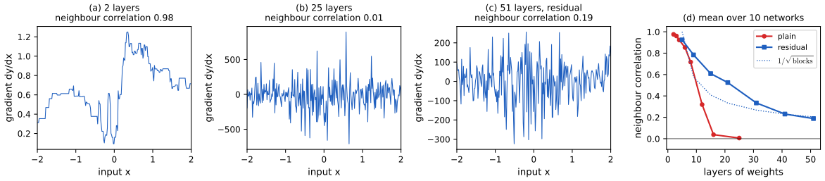
pp. 274–277 Depth gives networks much of their power, and careful initialisation (Section 7.2.5) and batch normalisation (Section 7.4.2) control vanishing and exploding gradients, yet very deep plain networks remain hard to train. One explanation is shattered gradients (Balduzzi et al., 2017): the number of linear regions of a ReLU network grows exponentially with depth (Result 6.5, Result 6.6), and with it the number of discontinuities of the gradient. For one input and one output, the derivative \(\d y/\d x\) of a deep network looks like noise (Figure 9.12), so tiny changes of the early weights change the gradient a lot, and gradient methods, which assume a gradient that varies smoothly, struggle.
A residual connection (He et al., 2015a) adds the input of a block to its output. A network of three layers
\[ \bz_1=F_1(\bx),\qquad\bz_2=F_2(\bz_1),\qquad\by=F_3(\bz_2) \tag{9.32–9.34} \]becomes a residual network (ResNet) of three residual blocks (Figure 9.13, a diagram of the chain \(\bx\to F_1\to+\to F_2\to+\to F_3\to+\to\by\) with the skip paths):
\[ \bz_1=F_1(\bx)+\bx, \tag{9.35} \] \[ \bz_2=F_2(\bz_1)+\bz_1, \tag{9.36} \] \[ \by=F_3(\bz_2)+\bz_2 . \tag{9.37} \]A block can represent the identity by making \(F_l\) small, and \(F_l\) learns the residual
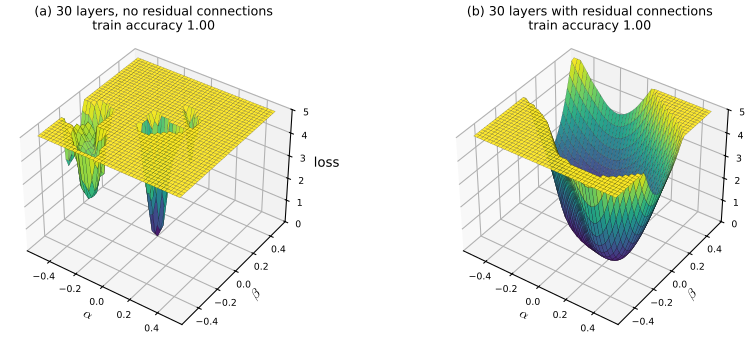
\[ F_l(\bz_{l-1})=\bz_l-\bz_{l-1}. \tag{9.38} \]Residual networks have much smoother error surfaces (Li et al., 2017; Figure 9.14) and, with batch normalisation, can be trained with hundreds of layers (He et al., 2015a). Substituting the blocks into each other gives
\[ \by=F_3(F_2(F_1(\bx)+\bx)+\bz_1)+\bz_2 \tag{9.39} \] \[ \by=F_3\big(F_2(F_1(\bx)+\bx)+F_1(\bx)+\bx\big)+F_2(F_1(\bx)+\bx)+F_1(\bx)+\bx \tag{9.40} \](Exercise 9.13). Figure 9.15 of the book draws (9.40) as a set of sub-networks in parallel, from the direct path \(\bx\) to the full depth-3 chain: the network can represent a deep function, but its error surface is moderated by the shallow paths. Changing the dimension between blocks needs a learned matrix on the skip path,
\[ \bz_l=F_l(\bz_{l-1})+\bW\bz_{l-1}. \tag{9.41} \]With \(F_l\) made of linear layers and ReLUs there are two places to put the addition (Figure 9.16, a diagram): after a ReLU (version (a), so only non-negative values are added) or after a linear layer, with the ReLU at the start of the branch (version (b), "pre-activation", which can add values of both signs and is more common).
Result 9.10 (the unrolled residual network and its Jacobian) pp. 275–277, (9.35)–(9.40); Exercise 9.13
For \(L\) blocks \(\bz_l=F_l(\bz_{l-1})+\bz_{l-1}\), \(\bz_0=\bx\), with Jacobians \(\bJ_l=\partial F_l/\partial\bz\) evaluated at \(\bz_{l-1}\):
- \(\bz_L=\bx+\sum_{l=1}^LF_l(\bz_{l-1})\); for \(L=3\), substituting gives (9.40).
- \[\dfrac{\partial\bz_L}{\partial\bx}=(\bI+\bJ_L)\cdots(\bI+\bJ_1)=\sum_{S\subseteq\{1,\dots,L\}}\ \prod_{l\in S}^{\leftarrow}\bJ_l,\] a sum over all \(2^L\) paths through the network, \(\binom Lk\) of them of depth \(k\), including the identity path \(S=\varnothing\). The error gradient reaching block \(l\) is \[\frac{\partial E}{\partial\bz_l}=\frac{\partial E}{\partial\bz_L}\prod_{k>l}(\bI+\bJ_k),\] which also contains the direct term \(\partial E/\partial\bz_L\).
- If \(\|\bJ_l\|\le\varepsilon\) for all \(l\) (spectral norm), every singular value of \(\partial\bz_L/\partial\bx\) lies in \([\,2-(1+\varepsilon)^L,\,(1+\varepsilon)^L\,]\). With \(\varepsilon\le c/L\) the bounds are \(2-e^c\) and \(e^c\), independent of depth.
Proof
(1) Sum (9.38) over \(l\): the right side telescopes to \(\bz_L-\bz_0\). For \(L=3\), substitute (9.35) into (9.36) and the result into (9.37): \(\bz_2=F_2(F_1(\bx)+\bx)+F_1(\bx)+\bx\), and \(\by=F_3(\bz_2)+\bz_2\) with this \(\bz_2\) is (9.40) (checked numerically for random blocks).
(2) By the chain rule, \(\partial\bz_l/\partial\bz_{l-1}=\bJ_l+\bI\), and the Jacobian of the composition is the product. Expanding a product of \(L\) binomials \((\bI+\bJ_l)\) (keeping the order, since the matrices do not commute) gives one term for each choice, in every factor, of \(\bI\) or \(\bJ_l\): the term is the ordered product of the chosen \(\bJ\)s (checked for \(L=4\): the 16 terms add up to the product). The backward statement is the transpose of the same product.
(3) The terms with \(|S|=k\ge1\) have norm at most \(\varepsilon^k\) (submultiplicativity), so \[\|\prod(\bI+\bJ_l)-\bI\|\le\sum_{k\ge1}\binom Lk\varepsilon^k=(1+\varepsilon)^L-1.\] For any matrix \(\bm A\), the singular values of \(\bI+\bm A\) lie in \([1-\|\bm A\|,1+\|\bm A\|]\) (Weyl's inequality). With \(\varepsilon\le c/L\), \((1+c/L)^L\le e^c\). ∎
Contrast a plain network: its Jacobian is \(\bJ_L\cdots\bJ_1\), a single path of full depth, whose norm can be as small as the product of the smallest singular values; with \(\|\bJ_l\|\le\varepsilon<1\) it is at most \(\varepsilon^L\), which vanishes exponentially. In a residual network the short paths keep the gradient informative even when the long ones are small or erratic, and if the residual branches start small the network starts close to the identity, which is easy to optimise (checked: bounds hold for random blocks with \(L=3,8,20\)).
Filling the gap 9.10: shattering, and why residual networks shatter slowly (a heuristic) pp. 274–275, Figure 9.12
The book shows the effect; here is a measurable version and the reason behind the residual curve in Figure 9.12(d).
Argument
Measure. Let \(g(x)=\d y/\d x\) on a fine grid. Its neighbour correlation \(\sum_k\tilde g_k\tilde g_{k+1}/\sum_k\tilde g_k^2\) (with \(\tilde g=g-\bar g\)) is close to 1 for a smooth gradient and close to 0 for white noise. In a ReLU network, \(g(x)\) is the product of the layers' weight matrices restricted to the units active at \(x\). Each layer with normalised pre-activations switches about half its units on and off across the inputs, so between two neighbouring inputs each layer changes some of its activity pattern; the products along two nearby inputs share fewer and fewer factors as depth grows, and their correlation decays roughly geometrically (measured: 0.98 at 2 layers, 0.32 at 12, 0.04 at 16, 0.01 at 25).
Residual networks. With normalisation inside each branch, each block adds to the stream a contribution of roughly fixed size, so after \(l\) blocks the stream is a sum of \(l\) comparable terms and its squared size grows linearly in \(l\). The gradient of the output is a sum over paths (Result 9.10); the paths through few blocks are smooth in \(x\), those through many are shattered, and their relative weights make the correlation decay like a power of the depth rather than exponentially. Balduzzi et al. (2017) derive the rate \(1/\sqrt L\) for this architecture; the measured curve of Figure 9.12(d) follows it closely (0.19 at 24 blocks against \(1/\sqrt{24}=0.20\)). This is a heuristic, not a proof: the exact rate depends on the initialisation and the normalisation. ∎
9.6 Model Averaging
See also the companion course, Section 14.2 (committees; Result 14.2, Filling the gap 14.3 on why bagged errors are correlated, Algorithm 14.1 bagging) and Section 14.3 (boosting), with the trees and committees demo.
pp. 277–279 Averaging the predictions of several trained models (a committee or ensemble) usually beats choosing the best one. For probabilistic outputs,
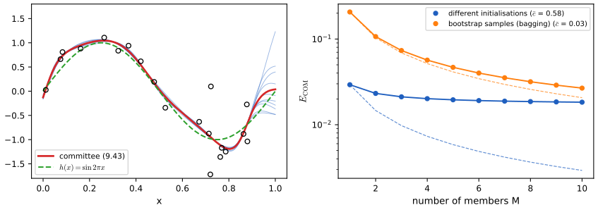
\[ p(y\given\bx)=\frac1L\sum_{l=1}^Lp_l(y\given\bx). \tag{9.42} \]The motivation is the variance term of the bias–variance decomposition, which averaging cancels (Figure 4.7). With one data set, variety between the models has to be created: by training on bootstrap data sets of \(N\) points drawn with replacement (bagging, Breiman, 1996), by different architectures, or (as in deep learning) by different random initialisations. For a regression output, write the committee prediction and the errors of its members as
\[ y_{\rm COM}(\bx)=\frac1M\sum_{m=1}^My_m(\bx), \tag{9.43} \] \[ y_m(\bx)=h(\bx)+\epsilon_m(\bx), \tag{9.44} \]with \(h\) the true function, so that
\[ \E_{\bx}\big[\{y_m(\bx)-h(\bx)\}^2\big]=\E_{\bx}\big[\epsilon_m(\bx)^2\big], \tag{9.45} \] \[ \Eav=\frac1M\sum_{m=1}^M\E_{\bx}\big[\epsilon_m(\bx)^2\big], \tag{9.46} \] \[ \Ecom=\E_{\bx}\Big[\Big\{\frac1M\sum_{m=1}^My_m(\bx)-h(\bx)\Big\}^2\Big]=\E_{\bx}\Big[\Big\{\frac1M\sum_{m=1}^M\epsilon_m(\bx)\Big\}^2\Big]. \tag{9.47} \]If the errors have zero mean and are uncorrelated,
\[ \E_{\bx}[\epsilon_m(\bx)]=0, \tag{9.48} \] \[ \E_{\bx}[\epsilon_m(\bx)\epsilon_l(\bx)]=0,\quad m\ne l, \tag{9.49} \]then
\[ \Ecom=\frac1M\Eav . \tag{9.50} \]In practice the errors are highly correlated and the gain is much smaller, but the committee is never worse than its average member (Exercise 9.15). The next result makes both statements exact.
Result 9.11 (committee error: correlations, Jensen and the ambiguity decomposition) pp. 278–279, (9.43)–(9.50); Exercises 9.14–9.16
Let \(C_{ml}=\E_{\bx}[\epsilon_m\epsilon_l]\), so \(\Eav=\frac1M\sum_mC_{mm}\), and define the average error correlation \(\bar c\) by \(\bar c\,\Eav=\frac1{M(M-1)}\sum_{m\ne l}C_{ml}\).
- \[\Ecom=\frac1{M^2}\sum_{m,l}C_{ml}=\Eav\big(\bar c+\frac{1-\bar c}M\big).\] With (9.48)–(9.49), \(\bar c=0\) and this is (9.50) (Exercise 9.14).
- From a pool of \(M\) trained models, the committee of \(m\) members chosen at random has expected error exactly \(\Eav(\bar c+(1-\bar c)/m)\), with \(\Eav,\bar c\) computed on the pool.
- (Ambiguity decomposition; Krogh and Vedelsby, 1995.) \[\Ecom=\Eav-\E_{\bx}\big[\frac1M\sum_m(y_m-y_{\rm COM})^2\big].\] In particular \(\Ecom\le\Eav\) (9.64), with equality iff all members agree almost everywhere (Exercise 9.15).
- For any error \(\mathcal E(y)\) convex in the prediction, \(\mathcal E(y_{\rm COM})\le\frac1M\sum_m\mathcal E(y_m)\) pointwise and hence in expectation (Exercise 9.16).
Proof
(1) Expand the square in (9.47): \(\big(\frac1M\sum_m\epsilon_m\big)^2=\frac1{M^2}\sum_{m,l}\epsilon_m\epsilon_l\), and take \(\E_{\bx}\). Split into the \(M\) diagonal terms, summing to \(M\Eav\), and the \(M(M-1)\) off-diagonal ones, summing to \(M(M-1)\bar c\Eav\); divide by \(M^2\). (The zero-mean assumption (9.48) is not needed for (9.50): uncorrelated in the sense \(\E[\epsilon_m\epsilon_l]=0\) suffices.)
(2) Choose a subset \(S\) of size \(m\) uniformly. Each index is in \(S\) with probability \(m/M\), each ordered pair of distinct indices with probability \(m(m-1)/(M(M-1))\). So \(\E_S\sum_{i,j\in S}C_{ij}=m\Eav+m(m-1)\bar c\Eav\), and dividing by \(m^2\) gives the formula (checked exactly over all 1023 subsets of 10 trained networks).
(3) For numbers \(a_1,\dots,a_M\) with mean \(\bar a\), \(\frac1M\sum_ma_m^2=\bar a^2+\frac1M\sum_m(a_m-\bar a)^2\). With \(a_m=\epsilon_m(\bx)\), \(\bar a=y_{\rm COM}-h\) and \(a_m-\bar a=y_m-y_{\rm COM}\); take \(\E_{\bx}\). The last term is non-negative, which gives (9.64); this is also Jensen's inequality for \(f(x)=x^2\) with weights \(1/M\), the manual's route.
(4) Jensen's inequality \(\mathcal E\big(\frac1M\sum_my_m\big)\le\frac1M\sum_m\mathcal E(y_m)\) at each \(\bx\) (and each target), then take expectations (checked for the absolute, logistic and quartic errors). ∎
What averaging cannot remove: if \(\epsilon_m=b+\delta_m\) with a common bias \(b(\bx)\) and uncorrelated zero-mean \(\delta_m\), then \(\Ecom=\E[b^2]+\frac1M\E[\overline{\delta^2}]\): only the variance part is divided by \(M\). The ambiguity term shows the trade-off in ensemble design: members should be individually good and disagree.
Filling the gap 9.11: what a bootstrap sample contains p. 278
A bootstrap sample of size \(N\) contains on average a fraction \(1-(1-1/N)^N\) of the distinct original points, which decreases to \(1-1/e\approx0.632\).
Derivation
A given point is missed by one draw with probability \(1-1/N\) and by all \(N\) independent draws with probability \((1-1/N)^N\); by linearity of expectation the expected fraction of points present is \(1-(1-1/N)^N\) (0.636 for \(N=50\), checked by simulation). Since \[\ln(1-1/N)^N=N\ln(1-1/N)=-1-\frac1{2N}-\frac1{3N^2}-\cdots\] increases to \(-1\), \((1-1/N)^N\) increases to \(e^{-1}\). Each bagged model therefore never sees about a third of the data, which both decorrelates the members (Result 9.11) and gives a free validation set for each member (out-of-bag error). ∎
p. 279 Boosting (Freund and Schapire, 1996) is different: base classifiers are trained in sequence, each on a data set reweighted to emphasise the points its predecessors got wrong, and combined by weighted majority vote; it works even with base classifiers only slightly better than chance (companion Section 14.3). All model combination multiplies the cost of training and prediction.
9.6.1 Dropout
pp. 279–281 Dropout (Srivastava et al., 2014) is a cheap, implicit average over exponentially many networks. Each time a data point is presented, every non-output unit (hidden and input) is deleted with its connections at random: its output is multiplied by a mask \(R_i\in\{0,1\}\) equal to 1 with probability \(\rho\) (about 0.5 for hidden units, 0.8 for inputs), drawn afresh for each point. Forward and backward propagation run on the thinned network, and the gradients are averaged over the mini-batch. With \(M\) non-output units there are \(2^M\) thinned networks; unlike an ordinary ensemble they share their weights and are never trained individually to convergence. Training is noisier and slower, and the noisy error is harder to monitor. At test time the ideal prediction is the ensemble average
\[ p(y\given\bx)=\sum_{\bR}p(\bR)\,p(y\given\bx,\bR), \tag{9.51} \]approximated by sampling 10 to 20 masks (Monte Carlo dropout) or, more simply, by using the full network with each unit's outgoing weights multiplied by \(\rho\) (weight scaling), so that each unit receives at test time the input it received on average in training. The Bayesian reading: (9.51) gives every sub-network equal weight, a crude stand-in for weighting by posterior probability. Dropout also prevents co-adaptation: a unit cannot rely on particular other units being present. For linear regression it is a modified quadratic regulariser (Exercise 9.18).
Result 9.12 (dropout on a linear model is a data-dependent ridge penalty) p. 281; Exercise 9.18, (9.68)–(9.73)
For \(y_k=\sum_{i=1}^Dw_{ki}x_i\) (9.68) with input dropout, \[ E(\bW)=\sum_{n=1}^N\sum_{k=1}^K\Big\{t_{nk}-\sum_{i=1}^Dw_{ki}R_{ni}x_{ni}\Big\}^2 , \tag{9.69} \] and independent \(R_{ni}\sim\mathrm{Bern}(\rho)\), we have \(\E[R_{ni}]=\rho\) (9.70), \(\E[R_{ni}R_{nj}]=\delta_{ij}\rho+(1-\delta_{ij})\rho^2\) (9.71), and \[ \E[E(\bW)]=\sum_{n=1}^N\sum_{k=1}^K\Big\{t_{nk}-\rho\sum_{i=1}^Dw_{ki}x_{ni}\Big\}^2+\rho(1-\rho)\sum_{n=1}^N\sum_{k=1}^K\sum_{i=1}^Dw_{ki}^2x_{ni}^2 . \tag{9.72–9.73} \]
Erratum: the book's (9.72) has \(y_{nk}\) where the target \(t_{nk}\) is meant. With \(\bD=\diag(\bX^\T\bX)\), the minimiser is \[ \bW^\star=\bT^\T\bX\big(\rho\,\bX^\T\bX+(1-\rho)\bD\big)^{-1}, \] and the test-time (weight-scaled) weights \(\rho\bW^\star=\bT^\T\bX\big(\bX^\T\bX+\frac{1-\rho}\rho\bD\big)^{-1}\) are ridge regression with a separate coefficient \(\frac{1-\rho}\rho\sum_nx_{ni}^2\) for each input. For standardised inputs (\(\bD=N\bI\)) it is ordinary ridge with \(\lambda=N(1-\rho)/\rho\).
Proof
Moments. \(\E[R]=0\cdot(1-\rho)+1\cdot\rho=\rho\). For \(i\ne j\), independence gives \(\E[R_iR_j]=\rho^2\); for \(i=j\), \(R_i^2=R_i\) so \(\E[R_i^2]=\rho\). Together this is (9.71).
Expected error. Fix \(n,k\) and let \(A=\sum_iw_{ki}R_{ni}x_{ni}\). Then \(\E[A]=\rho\sum_iw_{ki}x_{ni}\) and, the \(R_{ni}\) being independent, \[\var[A]=\sum_iw_{ki}^2x_{ni}^2\var[R_{ni}]=\rho(1-\rho)\sum_iw_{ki}^2x_{ni}^2.\] Since \(\E[(t-A)^2]=(t-\E A)^2+\var A\), summing over \(n,k\) gives (9.72)–(9.73) (checked against the exact average over all 16 masks of a 4-input model).
Minimiser. In matrix form the expected error is \(\|\bT-\rho\bX\bW^\T\|^2+\rho(1-\rho)\Tr(\bW\bD\bW^\T)\), whose gradient with respect to \(\bW\) is \(-2\rho(\bT-\rho\bX\bW^\T)^\T\bX+2\rho(1-\rho)\bW\bD\). Setting it to zero: \(\bT^\T\bX=\bW(\rho\bX^\T\bX+(1-\rho)\bD)\). The matrix in brackets is positive definite when \(\rho<1\) and no input is identically zero, so the solution is unique and the objective strictly convex. Multiplying by \(\rho\) and dividing inside the inverse by \(\rho\) gives the ridge form. ∎
Erratum (solutions manual). The manual's final answer \(\bW^\star=\bm B\bm M^{-1}\) uses a diagonal \(\bm B\) with \(B_{ii}=-2\rho\sum_nx_{ni}\): the targets \(t_{nk}\) have disappeared from the derivative and the sign is reversed, so for \(K\ne D\) the matrix \(\bm B\) does not even have the shape \(K\times D\) of \(\bW\). The correct first factor is \(\bm B=2\rho\,\bT^\T\bX\), which gives the formula above (whose gradient is zero to \(10^{-15}\); stochastic training with fresh masks converges to it, Figure 9.S4).
Result 9.13 (when weight scaling is exact) pp. 280–281, (9.51)
- If the output is linear in the masked units (dropout on the inputs of a linear layer, or on the last hidden layer before linear outputs), the average over all masks of the output equals the output of the network with the outgoing weights of the masked units multiplied by \(\rho\). So weight scaling computes the mean of the ensemble (9.51) exactly.
- For a softmax output layer \(p(y=k\given\bx,\bR)=\mathrm{softmax}_k(\bW(\bR\odot\bz))\) with dropout on its inputs \(\bz\), the normalised geometric mean of the \(2^M\) sub-network predictions, \(\exp\{\E_{\bR}\ln p(k\given\bx,\bR)\}\) renormalised over \(k\), equals \(\mathrm{softmax}_k(\rho\bW\bz)\) exactly.
- With nonlinear layers between the masks and the output, neither holds exactly: weight scaling is an approximation and Monte Carlo dropout with \(K\) masks is an unbiased estimate of (9.51) whose variance falls like \(1/K\).
Proof
(1) \[\E_{\bR}\big[\sum_jv_jR_jz_j\big]=\sum_jv_j\E[R_j]z_j=\sum_j(\rho v_j)z_j,\] by linearity of expectation (checked by enumerating all \(2^6\) masks).
(2) Let \(a_k(\bR)=\sum_jW_{kj}R_jz_j\). Then \(\ln p(k\given\bR)=a_k(\bR)-\ln\sum_le^{a_l(\bR)}\). Averaging over masks, \[\E_{\bR}\ln p(k\given\bR)=\rho\sum_jW_{kj}z_j-\E_{\bR}\ln\sum_le^{a_l(\bR)}.\] The second term does not depend on \(k\), so it cancels when the geometric mean is renormalised over \(k\), leaving \(e^{\rho(\bW\bz)_k}/\sum_le^{\rho(\bW\bz)_l}\) (Baldi and Sadowski, 2013; checked by enumerating all \(2^8\) masks, while the arithmetic mean (9.51) differs from it by up to 0.05 in probability).
(3) The average of \(K\) independent draws of \(p(y\given\bx,\bR)\) has mean (9.51) and variance \(\var_{\bR}[p(y\given\bx,\bR)]/K\). ∎
Training conventions differ: many libraries use inverted dropout, multiplying the kept units by \(1/\rho\) during training so that no scaling is needed at test time; the two are equivalent reparametrisations.
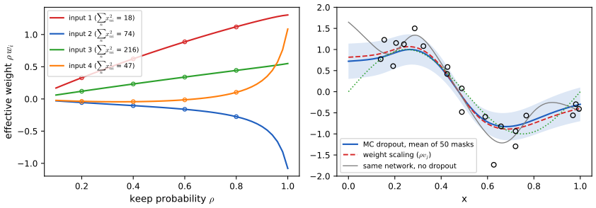
Figure 9.17 of the book (a network and two of its thinned versions, a drawing) is not reproduced.
Summary: errors found in the chapter (first printing) and in the solutions manual
- p. 263, after (9.14): the coefficients must be rescaled as \(\lambda_1\to a^2\lambda_1\), \(\lambda_2\to c^{-2}\lambda_2\), not \(a^{1/2}\lambda_1\), \(c^{-1/2}\lambda_2\) (Result 9.5; checked numerically).
- Figure 9.4: the panel labels behave as prior standard deviations, not precisions (Filling the gap 9.4).
- (9.28): \(\partial\wE/\partial\xi\) should be \(\partial\wE/\partial\xi_j\).
- p. 267: the text calls the learning rate \(\eta\), Exercise 9.6 calls it \(\rho\) and uses \(\eta_j\) for the eigenvalues; not wrong, but confusing.
- Exercise 9.3: \(\Omega(\bw)=-\frac12\bw^\T\bw\) should be \(+\frac12\bw^\T\bw\) (otherwise the weights grow), and (9.55) should read \(\bw^{(\tau+1)}=\bw^{(\tau)}-\eta\nabla\Omega\).
- (9.72): \(y_{nk}\) should be \(t_{nk}\) (Result 9.12).
- Solutions manual, 9.2: the added term is \(\frac{N\sigma^2}2\sum_iw_i^2\), not \(\frac{\sigma^2}2\sum_iw_i^2\) (Filling the gap 9.2; Monte Carlo: 4.31 against 4.34 and 0.17).
- Solutions manual, 9.3: starts from the printed \(\Omega=-\frac12\bw^\T\bw\) and obtains \(\d\bw/\d t=-\widetilde\eta\bw\), which is the result for \(+\frac12\bw^\T\bw\).
- Solutions manual, 9.11: computes \(\partial\Omega/\partial\sigma_j\) and states that this gives (9.28), which is a derivative with respect to \(\xi_j\); the missing factor \(\partial\sigma_j/\partial\xi_j=\sigma_j/2\) does give (9.28).
- Solutions manual, 9.12: a broken cross-reference "(??)".
- Solutions manual, 9.17: claims \(y_{\min}<y_{\rm COM}<y_{\max}\) strictly for all other weights, false when members agree; the necessity argument is fine.
- Solutions manual, 9.18: the final closed form \(\bm B\bm M^{-1}\) with diagonal \(\bm B\) loses the targets and the sign; the correct solution is \[\bT^\T\bX(\rho\bX^\T\bX+(1-\rho)\diag(\bX^\T\bX))^{-1}\] (Result 9.12; gradient checked).
Exercises
All 18 exercises of Chapter 9 (Bishop and Bishop, 2024, pp. 281–285), restated in my own words, with complete solutions (hidden). Stars give the book's difficulty. Each was solved independently and then compared with the official solutions manual; where they differ, the solution says so and why.
Exercise 9.1 (★). Check the four group axioms for (a) the rotations of a square by multiples of \(90^\circ\) under composition, and (b) the continuous translations of the plane.
Solution
(a) Represent a rotation by its angle \(k\cdot90^\circ\), \(k\in\{0,1,2,3\}\) taken modulo 4. Composition adds angles: \(k_1+k_2\bmod4\) is again in the set (closure); addition modulo 4 is associative; \(k=0\) is the identity; the inverse of \(k\) is \(4-k\bmod4\) (a rotation by \(-90^\circ\) is one by \(270^\circ\)). (b) A translation is a vector \(\bm a\in\R^2\) acting by \(\bx\mapsto\bx+\bm a\); composition adds vectors, which is closed and associative, with identity \(\bzero\) and inverse \(-\bm a\). Both groups are commutative. (Checked with \(2\times2\) rotation matrices and cyclic shifts. Same as the manual.)
Exercise 9.2 (★★). For the linear model \(y=w_0+\sum_iw_ix_i\) (9.52) and \(E_D=\frac12\sum_n\{y(\bx_n,\bw)-t_n\}^2\) (9.53), add independent zero-mean noise of variance \(\sigma^2\) to every input and show that the expected error is \(E_D\) plus a weight-decay term that does not involve \(w_0\).
Solution
See the last paragraph of Filling the gap 9.2: \(\E[\widetilde E_D]=E_D+\frac{N\sigma^2}2\sum_{i=1}^Dw_i^2\). The cross term vanishes because \(\E[\epsilon_{ni}]=0\), the quadratic term gives \(\sum_iw_i^2\sigma^2\) per data point, and \(w_0\) multiplies no noise. The manual drops the factor \(N\) in its last line.
Exercise 9.3 (★★). Gradient descent on the regulariser alone, \(\Omega=\frac12\bw^\T\bw\) (the book prints a minus sign, an erratum): pass to the limit of infinitesimal steps, solve the differential equation from \(\bw_0\) and show that the weights decay exponentially.
Solution
Write the step as \(\bw(t+\delta)=\bw(t)-\delta\,\widetilde\eta\nabla\Omega\), with \(\widetilde\eta=\eta/\delta\) the learning rate per unit time. Taylor expanding the left side, \(\bw(t)+\delta\,\d\bw/\d t+O(\delta^2)\), and letting \(\delta\to0\): \(\d\bw/\d t=-\widetilde\eta\nabla\Omega=-\widetilde\eta\bw\). Each component satisfies \(\dot w_i=-\widetilde\eta w_i\), whose unique solution is \(w_i(t)=w_{0i}e^{-\widetilde\eta t}\): exponential decay to 0 at rate \(\widetilde\eta\). With the printed \(-\frac12\bw^\T\bw\), \(\nabla\Omega=-\bw\) and the solution would be \(\bw_0e^{+\widetilde\eta t}\). See Filling the gap 9.3.
Exercise 9.4 (★). Verify that (9.9)–(9.10) keep the network (9.6)–(9.7) unchanged under the input transformation (9.8), and that (9.12)–(9.13) produce the output transformation (9.11).
Solution
Part (1) of the proof of Result 9.5: the hidden pre-activations are unchanged term by term, \(\frac{w_{ji}}a(ax_i+b)\) contributing \(w_{ji}x_i+\frac baw_{ji}\), whose second part is cancelled by the bias shift; and \(\sum_jcw_{kj}z_j+cw_{k0}+d=cy_k+d\). (Checked numerically. The manual has the same argument, with some summation indices misprinted.)
Exercise 9.5 (★★). Using Lagrange multipliers, show that minimising (9.19) is equivalent to minimising \(E\) under the constraint (9.20), and discuss how \(\eta\) and \(\lambda\) are related.
Solution
Result 9.6. The Lagrangian of the constrained problem is \(E(\bw)+\frac\lambda2\big(\sum_j|w_j|^q-\eta\big)\) with multiplier \(\frac\lambda2\ge0\); the constant \(-\frac\lambda2\eta\) does not affect the minimiser, which is that of (9.19). When the constraint is active (\(\lambda>0\)) the solution lies on the boundary, \(\sum_j|\widehat w_j|^q=\eta\), which fixes \(\eta\) as a function of \(\lambda\). This map is non-increasing (proved in the result by an exchange argument): a larger penalty means a smaller region. Its exact form depends on \(E\). The direction "penalised \(\Rightarrow\) constrained" needs no assumptions; the converse needs convexity (\(q\ge1\), convex \(E\)). The manual gives the Lagrangian step and the qualitative relation.
Exercise 9.6 (★★★). For the quadratic (9.56) and gradient descent (9.57) from the origin, show (9.58) for the components along the eigenvectors (9.59), that \(\bw^{(\tau)}\to\bws\) when \(|1-\rho\eta_j|<1\), and the approximations (9.60)–(9.61) after finitely many steps, so that \((\rho\tau)^{-1}\) acts like \(\lambda\).
Solution
Result 9.7, parts (1) and (3), with the sharper two-sided bound (2): for \(0<\rho\eta_j\le1\), \(\frac{\eta_j}{\eta_j+\lambda}\le1-(1-\rho\eta_j)^\tau\le\frac{2\eta_j}{\eta_j+\lambda}\) with \(\lambda=1/(\rho\tau)\). The manual proves (9.58) by induction and argues (9.61) with \((1-\rho\eta_j)^\tau=1-\tau\rho\eta_j+O(\rho\eta_j^2)\); the remainder should be \(O(\tau^2\rho^2\eta_j^2)\), which is small precisely when \(\rho\eta_j\tau\ll1\). Our bounds avoid the approximation.
Exercise 9.7 (★★). How must backpropagation be modified when several weights are constrained to be equal?
Solution
Filling the gap 9.9: compute \(\partial E/\partial w_i\) for every connection as if all were free, then add them within each group to get the derivative with respect to the shared parameter; update the shared parameter (all members) with that sum. Members initialised equal stay equal. (Same as the manual.)
Exercise 9.8 (★). Treating \(\pi_j\) as prior probabilities in the mixture \(p(w)=\sum_j\pi_j\N(w\given\mu_j,\sigma_j^2)\) (9.62), show by Bayes' theorem that the posterior probabilities are (9.24).
Solution
With \(p(j)=\pi_j\) and \(p(w\given j)=\N(w\given\mu_j,\sigma_j^2)\), the sum rule gives \(p(w)=\sum_kp(k)p(w\given k)\), which is (9.62), and Bayes' theorem gives \(p(j\given w)=p(j)p(w\given j)/p(w)\), which is (9.24). The posteriors sum to 1 over \(j\). (Same as the manual; checked numerically.)
Exercise 9.9 (★★). Derive (9.25) from (9.21)–(9.24).
Solution
Proof of Result 9.9, paragraph (9.25). (Same as the manual, which has \(\sigma^2\) for \(\sigma_j^2\) in one place.)
Exercise 9.10 (★★). Derive (9.26).
Solution
Proof of Result 9.9, paragraph (9.26): \(\mu_j\) appears in every \(Z_i\), and \(\partial\N_{ij}/\partial\mu_j=\N_{ij}(w_i-\mu_j)/\sigma_j^2\). (Same as the manual.)
Exercise 9.11 (★★). Derive (9.28).
Solution
Proof of Result 9.9, paragraph (9.28), differentiating with respect to \(\sigma_j^2\) and using \(\partial\sigma_j^2/\partial\xi_j=\sigma_j^2\). The manual differentiates with respect to \(\sigma_j\), obtaining \(\sum_i\gamma_j(w_i)\{1/\sigma_j-(w_i-\mu_j)^2/\sigma_j^3\}\), and then asserts (9.28) without the chain-rule factor \(\partial\sigma_j/\partial\xi_j=\sigma_j/2\), which is what converts one into the other.
Exercise 9.12 (★★). Show (9.63) for the softmax (9.30), and use \(\sum_k\gamma_k(w_i)=1\) to derive (9.31).
Solution
Proof of Result 9.9, paragraph (9.31). By the quotient rule, \(\partial\pi_k/\partial\eta_j=\frac{\delta_{jk}e^{\eta_k}}{\sum_le^{\eta_l}}-\frac{e^{\eta_k}e^{\eta_j}}{(\sum_le^{\eta_l})^2}=\delta_{jk}\pi_j-\pi_j\pi_k\) (checked by finite differences). (Same as the manual, which writes \(\delta_{jk}\pi_k\), equal because of the delta, and has a broken reference.)
Exercise 9.13 (★). Combine (9.35)–(9.37) into the single expression (9.40).
Solution
Proof of Result 9.10, part (1): substitute \(\bz_1\) into \(\bz_2\) and \(\bz_2\) into \(\by\). (Same as the manual; checked numerically with random blocks.)
Exercise 9.14 (★★). From (9.46)–(9.49), derive \(\Ecom=\Eav/M\) (9.50).
Solution
Part (1) of Result 9.11 with \(\bar c=0\): expanding the square, the cross terms vanish by (9.49) and the \(M\) diagonal terms give \(M\Eav/M^2\). (Same as the manual; checked by Monte Carlo, ratio 0.998.)
Exercise 9.15 (★★). Using Jensen's inequality for \(f(x)=x^2\), show \(\Ecom\le\Eav\) (9.64).
Solution
Part (3) of Result 9.11: pointwise \(\big(\frac1M\sum_m\epsilon_m\big)^2\le\frac1M\sum_m\epsilon_m^2\), with the exact gap \(\frac1M\sum_m(y_m-y_{\rm COM})^2\); take \(\E_{\bx}\). (Same route as the manual, plus the identity for the gap.)
Exercise 9.16 (★★). Show that (9.64) holds for any error \(E(y)\) that is convex in \(y\).
Solution
Part (4) of Result 9.11: Jensen's inequality \[E\big(\frac1M\sum_my_m(\bx)\big)\le\frac1M\sum_mE(y_m(\bx))\] at every \(\bx\) (and target), then take expectations. Examples: absolute error, cross-entropy as a function of the logit. (Same as the manual.)
Exercise 9.17 (★★). For a weighted committee \(y_{\rm COM}=\sum_m\alpha_my_m\) (9.65), show that requiring \(y_{\min}(\bx)\le y_{\rm COM}(\bx)\le y_{\max}(\bx)\) (9.66) for all possible member predictions is equivalent to \(\alpha_m\ge0\) and \(\sum_m\alpha_m=1\) (9.67).
Solution
Sufficiency. If (9.67) holds, \(y_{\rm COM}\) is a convex combination: \(y_{\rm COM}=\sum_m\alpha_my_m\le\sum_m\alpha_my_{\max}=y_{\max}\), and likewise \(\ge y_{\min}\).
Necessity. Suppose (9.66) holds whatever the members predict. Take all \(y_m=1\): then \(y_{\min}=y_{\max}=1\) forces \(\sum_m\alpha_m=1\). Take \(y_k=1\) and \(y_m=0\) for \(m\ne k\): then \(y_{\min}=0\le y_{\rm COM}=\alpha_k\). So every \(\alpha_k\ge0\).
The quantifier matters: for one fixed set of member predictions, other weights may also satisfy (9.66). The manual's necessity argument is the same; its sufficiency paragraph claims strict inequalities for all other settings of \(\alpha\), which fails when members agree (checked: a weight vector \((1.3,-0.3,0,\dots)\) violates (9.66) for some predictions).
Exercise 9.18 (★★★). For the linear model (9.68) with input dropout and error (9.69), show (9.70)–(9.71), derive the expected error (9.72)–(9.73), interpret it, and find the minimising weights in closed form.
Solution
Result 9.12: the expected error is the sum of squares of the model with weights scaled by \(\rho\) plus \(\rho(1-\rho)\sum_{n,k,i}w_{ki}^2x_{ni}^2\), a quadratic regulariser with one coefficient per input proportional to that input's sum of squares; the minimiser is \[\bW^\star=\bT^\T\bX(\rho\bX^\T\bX+(1-\rho)\diag(\bX^\T\bX))^{-1}.\] The book's (9.72) should have \(t_{nk}\) in place of \(y_{nk}\); the manual's expected error (its (381)) is right, but its final closed form \(\bm B\bm M^{-1}\) drops the targets from \(\bm B\) (see the erratum in the result's proof).
Demonstrations
Three interactive pages, each linked above where its topic arises. They run in the browser and reproduce the Python code. Lasso and ridge coefficients agree to \(1.3\times10^{-15}\), the learning curves of the early-stopping demo to \(2\times10^{-15}\) (relative), and the dropout run to \(5\times10^{-12}\). The ensemble presets train each member for 2000 steps of Adam with a constant step; near an interpolating fit Adam amplifies rounding differences between JavaScript and numpy (the two agree to \(10^{-14}\) after 500 steps), so after 2000 steps the reported errors agree to 1%.
- L1 versus L2 regularisation: paths and sparsity: lasso and ridge paths for eight inputs, the validation error, and the constrained minimum inside \(\sum|w_j|^q\le\eta\) for any \(q\). Presets: 1 ridge, 2 lasso, exact zeros, 3 correlated inputs, 4 few data, 5 \(q=0.5\).
- Early stopping versus weight decay: learning curves of a tanh network trained live, the network at any step, training with weight decay instead, and the quadratic case with both filters. Presets: 1 learning curves (Fig 9.7), 2 over-fitting, 3 weight decay, 4 the clock is \(\rho\tau\), 5 quadratic (Fig 9.8).
- Dropout and ensembles: committees of networks from different starts or bootstrap samples, with the correlation formula, and dropout with weight scaling and Monte Carlo averaging. Presets: 1 different starts, 2 bagging, 3 dropout \(\rho=0.8\), 4 strong dropout, 5 number of masks.
References
- Bishop, C. M. and Bishop, H. (2024). Deep Learning: Foundations and Concepts. Springer, Cham. Chapter 9, pp. 253–285. doi:10.1007/978-3-031-45468-4. Book website: www.bishopbook.com.
- Bishop, C. M. and Bishop, H. (2024). Deep Learning: Foundations and Concepts, Solutions to Exercises, version 1.0 (Chapters 2–10).
- Baldi, P. and Sadowski, P. (2013). Understanding dropout. In Advances in Neural Information Processing Systems 26.
- Balduzzi, D., Frean, M., Leary, L., Lewis, J. P., Ma, K. W.-D. and McWilliams, B. (2017). The shattered gradients problem: if resnets are the answer, then what is the question? In Proceedings of the 34th International Conference on Machine Learning, 342–350.
- Belkin, M., Hsu, D., Ma, S. and Mandal, S. (2019). Reconciling modern machine-learning practice and the classical bias–variance trade-off. Proceedings of the National Academy of Sciences, 116(32), 15849–15854. doi:10.1073/pnas.1903070116.
- Belkin, M., Hsu, D. and Xu, J. (2020). Two models of double descent for weak features. SIAM Journal on Mathematics of Data Science, 2(4), 1167–1180.
- Bishop, C. M. (1995). Training with noise is equivalent to Tikhonov regularization. Neural Computation, 7(1), 108–116. doi:10.1162/neco.1995.7.1.108.
- Breiman, L. (1996). Bagging predictors. Machine Learning, 24, 123–140.
- Freund, Y. and Schapire, R. E. (1996). Experiments with a new boosting algorithm. In Proceedings of the 13th International Conference on Machine Learning, 148–156.
- He, K., Zhang, X., Ren, S. and Sun, J. (2015a). Deep residual learning for image recognition. arXiv:1512.03385 (CVPR 2016).
- Heckel, R. and Yilmaz, F. F. (2021). Early stopping in deep networks: double descent and how to eliminate it. In International Conference on Learning Representations.
- Krogh, A. and Vedelsby, J. (1995). Neural network ensembles, cross validation, and active learning. In Advances in Neural Information Processing Systems 7, 231–238.
- Lasserre, J. A., Bishop, C. M. and Minka, T. P. (2006). Principled hybrids of generative and discriminative models. In Proceedings of the IEEE Conference on Computer Vision and Pattern Recognition.
- Leen, T. K. (1995). From data distributions to regularization in invariant learning. Neural Computation, 7(5), 974–981.
- Li, H., Xu, Z., Taylor, G., Studer, C. and Goldstein, T. (2017). Visualizing the loss landscape of neural nets. arXiv:1712.09913 (NeurIPS 2018).
- Mardia, K. V., Kent, J. T. and Bibby, J. M. (1979). Multivariate Analysis. Academic Press, London.
- Nakkiran, P., Kaplun, G., Bansal, Y., Yang, T., Barak, B. and Sutskever, I. (2019). Deep double descent: where bigger models and more data hurt. arXiv:1912.02292.
- Nowlan, S. J. and Hinton, G. E. (1992). Simplifying neural networks by soft weight-sharing. Neural Computation, 4(4), 473–493.
- Simard, P., Victorri, B., LeCun, Y. and Denker, J. (1992). Tangent prop: a formalism for specifying selected invariances in an adaptive network. In Advances in Neural Information Processing Systems 4, 895–903.
- Srivastava, N., Hinton, G., Krizhevsky, A., Sutskever, I. and Salakhutdinov, R. (2014). Dropout: a simple way to prevent neural networks from overfitting. Journal of Machine Learning Research, 15, 1929–1958.
- Tibshirani, R. (1996). Regression shrinkage and selection via the lasso. Journal of the Royal Statistical Society, Series B, 58(1), 267–288.
- Wolpert, D. H. (1996). The lack of a priori distinctions between learning algorithms. Neural Computation, 8(7), 1341–1390. doi:10.1162/neco.1996.8.7.1341.
- Yilmaz, F. F. and Heckel, R. (2022). Regularization-wise double descent: why it occurs and how to eliminate it. In IEEE International Symposium on Information Theory.
- Zhang, C., Bengio, S., Hardt, M., Recht, B. and Vinyals, O. (2016). Understanding deep learning requires rethinking generalization. arXiv:1611.03530.
Every numerical statement in these notes comes from ch09_regularization.py.