Neural Networks for Tabular Data
A multilayer perceptron composes affine maps with a nonlinearity, \(\bm z_l=\varphi(\bm W_l\bm z_{l-1}+\bm b_l)\), and ends in a linear layer whose output parametrises a likelihood: a Bernoulli or categorical distribution for classification, a Gaussian whose mean and variance are both outputs for regression, a mixture for one-to-many problems. Because every piece is differentiable, the gradient of the negative log-likelihood with respect to all parameters is obtained by one backward sweep, the vector-Jacobian products of reverse-mode automatic differentiation, at about twice the cost of the forward pass. The chapter then deals with what goes wrong in practice (gradients that vanish or explode with depth, saturating or dying units, bad initialisation) and the cures (non-saturating activations, residual connections, variance-preserving initialisation), with regularisation (early stopping, weight decay, sparsity, dropout, the implicit bias of stochastic gradient descent, over-parameterisation and double descent), and with two classical relatives of the MLP, radial basis function networks and mixtures of experts. The notes prove every statement the book leaves as "one can show" or as an exercise, correct a few slips in the book, and test the claims on small simulated problems and on MNIST.
Ch. 1 Introduction Ch. 2 Univariate probability Ch. 3 Multivariate probability Ch. 4 Statistics Ch. 5 Decision theory Ch. 6 Information theory Ch. 7 Linear algebra Ch. 8 Optimisation Ch. 9 Discriminant analysis Ch. 10 Logistic regression Ch. 11 Linear regression Ch. 12 GLMs Ch. 13 Networks for tabular data Ch. 14 Networks for images Ch. 15 Networks for sequences Ch. 16 Exemplar-based methods Ch. 17 Kernel methods Ch. 18 Trees and boosting Ch. 19 Fewer labels Ch. 20 Dimensionality reduction Ch. 21 Clustering Ch. 22 Recommender systems Ch. 23 Graph embeddings
How to read these notes
They follow the book. Sections carry the book's numbers (13.3.1, 13.4.5, ...) and equations the book numbers keep their numbers, e.g. \((13.69)\); equations without a number are steps the book skips. The book marks Sections 13.5.6 and 13.6 as optional (stars); they are covered in full here.
Filling the gaps. Wherever the book writes "one can show", leaves a step to an exercise, or quotes a result from the literature, an orange Filling the gap box gives the full argument. Proofs start hidden: open one with its bar, or use the buttons below.
Figures and demonstrations. Every computed figure is reproduced by the Python code. Figures 13.1b, 13.5, 13.8 to 13.13, 13.15, 13.16, 13.18, 13.19, 13.24 and 13.25 are drawings or photographs and Figure 13.9 is a table of historical network sizes: none is reproduced. Data: Figure 13.4 uses MNIST; all other data sets are simulated because the book's point sets are not available offline, and the captions say so. The ▶ Demo boxes open an interactive demonstration set to the case being discussed.
Main reference
K. P. Murphy, Probabilistic Machine Learning: An Introduction, MIT Press (2022), Chapter 13, pages 425–465 (book page: probml.github.io/pml-book/book1.html). Section, equation, figure and exercise numbers below refer to this book. The explanations, derivations, figures and code are my own.
Companion courses
Neural networks are developed, in other notation, elsewhere on this site. Where a result is proved in full there, these notes give the statement and a short sketch and link to it.
- Bayesian and Probabilistic Machine Learning (Bishop): 5.1 feed-forward network functions, 5.2 network training, 5.3 error backpropagation, 5.5 regularization in neural networks, 5.6 mixture density networks, 5.7 Bayesian neural networks; 6.3 radial basis function networks; 14.5 conditional mixture models.
- Foundations of Deep Learning (Bishop and Bishop): 6.2.2 universal approximation, 7.2.5 parameter initialization, 8.1 evaluation of gradients, 8.2 automatic differentiation, 9.2 weight decay, 9.3 learning curves, 9.5 residual connections, 9.6.1 dropout.
- Elements of Statistical Learning: 11.4 fitting neural networks, 11.5 some issues in training. Introduction to Statistical Learning: 10.7 fitting a neural network, 10.8 interpolation and double descent.
What this chapter adds: Murphy's vector-Jacobian-product account of reverse mode on general computation graphs, the heteroskedastic two-head regression network, the catalogue of non-saturating activations (ELU, SELU, swish, GELU), the variance-preserving initialisations, the modified-loss view of gradient descent, and the two classical relatives (RBF networks and mixtures of experts). The notes add: a full proof of universal approximation and of the depth separation by the sawtooth, the correct cost of forward-mode differentiation, a rigorous account of vanishing gradients and of residual connections, the derivation of the SELU constants, the exact regulariser induced by dropout, the proof of the modified loss for gradient descent and for shuffled SGD, and a closed-form double-descent curve.
The chapter at a glance
- 13.2.1–13.2.3 XOR by hand, every Boolean function by one hidden layer, and the collapse of linear networks (gap 13.1).
- 13.2.4 Example models; the heteroskedastic NLL (gap 13.2).
- 13.2.5 Universal approximation with a rate (gap 13.3); depth against width by the sawtooth and the count of linear regions (gap 13.4).
- 13.3 Reverse against forward mode, with the corrected cost (gap 13.5); backpropagation through an MLP and the VJPs of common layers (gap 13.6); adjoints on a DAG (gap 13.7).
- 13.4 Vanishing and exploding gradients (gap 13.8); the activation functions, dead ReLUs and the SELU constants (gap 13.9); residual connections (gap 13.10); Glorot, He and orthogonal initialisation (gap 13.11); data parallelism (gap 13.12).
- 13.5 Weight decay and early stopping as shrinkage filters (gap 13.13); l1 and proximal steps (gap 13.14); dropout as an adaptive penalty (gap 13.15); the modified loss of gradient descent and of SGD (gap 13.16); double descent in closed form (gap 13.17).
- 13.6 RBF networks, bandwidth and the XOR separation (gap 13.18); mixtures of experts, regression to the mean and EM (gap 13.19).
Notation. Inputs \(\bm x\in\R^D\); layer \(l\) has \(K_l\) units, weights \(\bm W_l\in\R^{K_l\times K_{l-1}}\), biases \(\bm b_l\), pre-activations \(\bm a_l=\bm b_l+\bm W_l\bm z_{l-1}\) and activations \(\bm z_l=\varphi_l(\bm a_l)\) with \(\bm z_0=\bm x\); \(\sigma\) is the sigmoid, \(\Heav\) the Heaviside step, \(\ReLU(a)=\max(a,0)\). The gradient \(\nabla_{\bm v}L\) has the shape of \(\bm v\) and is a column vector; the Jacobian of \(\bm f:\R^n\to\R^m\) is the \(m\times n\) matrix \(\bm J_f\). \(\NLL\) is the negative log-likelihood. Data matrices have one example per row in the code and one per column in formulas about single examples; the text says which.
Prerequisites. Chapters 7 and 8 of the book (matrix calculus, the chain rule, gradient descent, Adam), Chapters 10 and 11 (logistic and ridge regression), and the Gaussian and Bernoulli distributions of Chapters 2 and 3.
13.1 Introduction
pp. 425–426 Logistic regression, linear regression and the generalised linear models of Chapters 10 to 12 all assume that the input-output map is linear (in the logit, the mean, or the natural parameter). A first remedy is a fixed feature map \(\bm\phi\), giving \(f(\bm x;\bm\theta)=\bm W\bm\phi(\bm x)+\bm b\) (13.1): still linear in the parameters, so the NLL is still convex, but the features must be chosen by hand. The next step gives the feature extractor its own parameters, \(f(\bm x;\bm\theta)=\bm W\bm\phi(\bm x;\bm\theta_2)+\bm b\) (13.2), and repeats the idea recursively. Composing \(L\) functions, \[ f(\bm x;\bm\theta)=f_L(f_{L-1}(\cdots f_1(\bm x)\cdots)),\qquad f_\ell(\bm x)=f(\bm x;\bm\theta_\ell), \tag{13.3} \] gives a deep neural network; when the composition graph is a chain the model is a feedforward network or multilayer perceptron (MLP). An MLP takes a fixed-length vector as input, which is why it is the natural model for tabular data (an \(N\times D\) design matrix whose columns have a meaning); images, sequences and graphs get the specialised networks of Chapters 14, 15 and 23.
See also: Bayesian and Probabilistic ML, Section 5.1 (feed-forward network functions); Foundations of Deep Learning, Section 6.2 (multilayer networks).
13.2 Multilayer perceptrons (MLPs)
p. 426 A perceptron is the deterministic version of logistic regression (Section 10.2.5), \[ f(\bm x;\bm\theta)=\ind(\bm w^\T\bm x+b\ge0)=\Heav(\bm w^\T\bm x+b), \tag{13.4} \] with decision boundary a hyperplane. Minsky and Papert (1969) showed that this is very limiting; the standard example is XOR.
13.2.1 The XOR problem
pp. 427–428 The exclusive-or of two bits is \(y=x_1\oplus x_2\) (Table 13.1: it is 1 exactly when the bits differ). The four points are not linearly separable, but a network with one hidden layer of two perceptrons and one output perceptron computes it. With \(h_1=\Heav(x_1+x_2-1.5)\) (the AND), \(h_2=\Heav(x_1+x_2-0.5)\) (the OR) and \(y=\Heav(-h_1+h_2-0.5)\), i.e. \(y=\bar h_1\wedge h_2\), we get \(y=\overline{(x_1\wedge x_2)}\wedge(x_1\vee x_2)\) (13.6), which is XOR.
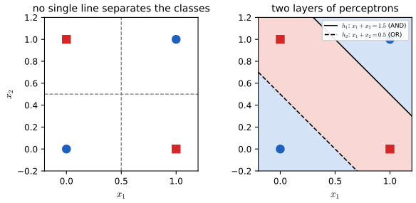
Filling the gap 13.1: XOR by hand, any Boolean function, and the collapse of linear networks pp. 427–428, (13.5), (13.10)
Derivation
The weights work. At \((0,0)\): \(h_1=\Heav(-1.5)=0\), \(h_2=\Heav(-0.5)=0\), \(y=\Heav(-0.5)=0\). At \((0,1)\) and \((1,0)\): \(h_1=0\), \(h_2=\Heav(0.5)=1\), \(y=\Heav(0.5)=1\). At \((1,1)\): \(h_1=\Heav(0.5)=1\), \(h_2=1\), \(y=\Heav(-0.5)=0\). (The book writes the step as \(\ind(a\ge0)\) in (13.4) and \(\ind(a>0)\) in Section 13.2.7; here no pre-activation is ever exactly 0, so the choice is immaterial.)
No perceptron computes XOR. Suppose \(\Heav(w_1x_1+w_2x_2+b)\) did. Then \(b<0\) (point \((0,0)\)), \(w_1+b\ge0\) and \(w_2+b\ge0\) (points \((1,0),(0,1)\)), and \(w_1+w_2+b<0\) (point \((1,1)\)). Adding the two middle inequalities gives \(w_1+w_2+2b\ge0\), hence \(w_1+w_2+b\ge-b>0\), contradicting the last one.
Any Boolean function of \(d\) bits is a one-hidden-layer perceptron network. For a pattern \(\bm p\in\{0,1\}^d\) let \(|\bm p|=\sum_ip_i\) and \(h_{\bm p}(\bm x)=\Heav\big(\sum_i(2p_i-1)x_i-|\bm p|+\tfrac12\big)\). For \(\bm x\in\{0,1\}^d\) the sum \(\sum_i(2p_i-1)x_i=\sum_{i:p_i=1}x_i-\sum_{i:p_i=0}x_i\) is an integer at most \(|\bm p|\), with equality exactly when \(\bm x=\bm p\). Hence \(h_{\bm p}(\bm x)=1\iff\bm x=\bm p\). For a Boolean function \(f\) take one hidden unit for each \(\bm p\) with \(f(\bm p)=1\) and the output \(\Heav(\sum_{\bm p}h_{\bm p}-\tfrac12)\), an OR. At most \(2^d\) hidden units are needed. (A confirmation for all 256 functions of three bits is in the code.)
Linear activations collapse (13.10). If \(\varphi_l(\bm a)=c_l\bm a\) for all \(l\) then \(\bm z_l=c_l(\bm W_l\bm z_{l-1}+\bm b_l)\) is an affine function of \(\bm z_{l-1}\), and a composition of affine maps is affine: by induction \(\bm z_L=\bm W'\bm x+\bm b'\) with \(\bm W'=\prod_lc_l\,\bm W_L\cdots\bm W_1\). With biases the collapsed model is affine rather than linear; without them it is exactly the \(\propto\) of (13.10). So a deep network with linear activations has the capacity of a single layer, and this is why a nonlinearity is essential. \(\square\)
13.2.2 Differentiable MLPs
p. 428 The Heaviside function has zero derivative almost everywhere, so a stack of perceptrons cannot be trained by gradients. Replace it by a differentiable activation \(\varphi:\R\to\R\) applied elementwise: \[ \bm z_l=f_l(\bm z_{l-1})=\varphi_l(\bm b_l+\bm W_l\bm z_{l-1}),\quad\text{in scalar form}\quad z_{kl}=\varphi_l\Big(b_{kl}+\sum_{j=1}^{K_{l-1}}w_{lkj}z_{jl-1}\Big), \tag{13.7, 13.8} \] and call \(\bm a_l=\bm b_l+\bm W_l\bm z_{l-1}\) the pre-activations (13.9), so \(\bm z_l=\varphi_l(\bm a_l)\). Composing \(L\) such layers as in (13.3) gives a function whose gradient with respect to every parameter is obtained by the chain rule, called backpropagation (Section 13.3). "MLP" nowadays always means this differentiable version.
13.2.3 Activation functions
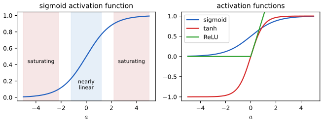
pp. 428–429 A nonlinear \(\varphi\) is essential (gap 13.1, last paragraph). The classical choices are the sigmoid \(\sigma(a)=1/(1+e^{-a})\) (13.11), a smooth approximation of the Heaviside step, and \(\tanh(a)=2\sigma(2a)-1\). Both saturate: for large \(|a|\) the output is nearly constant and the derivative nearly 0, so gradient signals cannot pass (the vanishing-gradient problem, Section 13.4.2). The most common choice today is the rectified linear unit \(\ReLU(a)=\max(a,0)=a\,\ind(a>0)\) (13.12), which zeroes negative inputs and passes positive ones unchanged. When a network represents a function on a continuous domain (a signal in time or space, a "neural implicit representation") ReLU networks are biased towards low frequencies; replacing ReLU by \(\sin\) helps (Sitzmann et al., 2020).
13.2.4 Example models
pp. 429–434 MLPs give classifiers and regressors for many kinds of data.
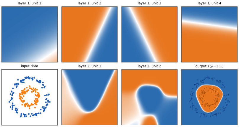
13.2.4.1 Two-dimensional data, two classes. The model of (13.13)–(13.16) is \(p(y\given\bm x;\bm\theta)=\operatorname{Ber}(y\given\sigma(a_3))\) with \(a_3=\bm w_3^\T\bm z_2+b_3\), \(\bm z_2=\varphi(\bm W_2\bm z_1+\bm b_2)\), \(\bm z_1=\varphi(\bm W_1\bm x+\bm b_1)\); the book's Figure 13.3 is a screenshot of an interactive tool. Figure 13.3 below is my own version: a \(2\)-\(4\)-\(2\)-\(1\) tanh network trained by Adam on 240 points drawn from two concentric circles (simulated; the book's points are not available). Each first-layer unit is a soft half-plane, the second layer combines them into a curved region, and the output is a closed boundary around the inner circle: precisely the carving-up described in Section 13.2.5.
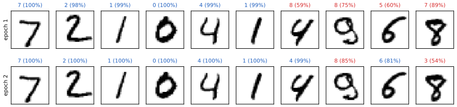
13.2.4.2 Image classification. To use an MLP on images, flatten each \(28\times28\) image to a vector in \(\R^{784}\). With two hidden layers of 128 units and a 10-way softmax output, the parameter count is \((784+1)\cdot128=100\,480\) for the first layer, \((128+1)\cdot128=16\,512\) for the second and \((128+1)\cdot10=1\,290\) for the third, in total \(118\,282\) (Table 13.2). Because the first layer treats pixels as unrelated inputs, permuting the pixels (the same permutation for every image) changes nothing about the model's capacity or training: an MLP has no knowledge of image structure, which is what convolutional networks (Chapter 14) exploit.
13.2.4.3 Text classification. Variable-length text is made fixed-length by a bag of words: an embedding matrix \(\bm W_1\in\R^{E\times V}\) maps each one-hot word \(\bm v_t\) to \(\bm e_t=\bm W_1\bm v_t\), the embeddings are averaged, \(\bm e=\frac1T\sum_t\bm e_t\) (global average pooling), and the average goes to an MLP: \(p(y\given\bm x;\bm\theta)=\operatorname{Ber}(y\given\sigma(\bm w_3^\T\bm h+b_3))\), \(\bm h=\varphi(\bm W_2\bm e+\bm b_2)\) (13.17)–(13.20). For \(V=10\,000\), \(E=16\) and a hidden layer of 16 units the parameters are \(160\,000\) (embedding) \(+\,16\cdot16+16=272\) \(+\,17\), in total \(160\,289\) (Table 13.3); most of them sit in the embedding matrix, which can instead be pre-trained without labels (Section 20.5), leaving only the last two layers to fit on the small labelled set.
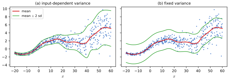
13.2.4.4 Heteroskedastic regression. Regression with an input-dependent noise level uses a shared backbone and two heads, one for the mean and one for the standard deviation (Figure 13.5, a drawing). The mean head is linear and the standard-deviation head goes through the softplus \(\sigma_+(a)=\log(1+e^a)\) so that it is positive: \[ p(y\given\bm x,\bm\theta)=\N\big(y\given\bm w_{\mu}^\T f(\bm x;\bm w_{\rm shared}),\ \sigma_+(\bm w_\sigma^\T f(\bm x;\bm w_{\rm shared}))\big). \tag{13.21} \] The second argument is the standard deviation (the book's notation is loose about whether it is a variance).
Filling the gap 13.2: the NLL of the two-head network and why a fixed variance is under-confident pp. 433–434, (13.21)
Derivation
Write the outputs of the network at \(\bm x_n\) as \(\mu_n\) and \(s_n\), \(\sigma_n=\sigma_+(s_n)\), \(r_n=y_n-\mu_n\). The mean NLL is \(\ell=\frac1N\sum_n\big[\tfrac12\log(2\pi\sigma_n^2)+\frac{r_n^2}{2\sigma_n^2}\big]\). Per example, \[ \frac{\partial\ell_n}{\partial\mu_n}=-\frac{r_n}{\sigma_n^2},\qquad \frac{\partial\ell_n}{\partial\sigma_n}=\frac1{\sigma_n}-\frac{r_n^2}{\sigma_n^3},\qquad \frac{\partial\ell_n}{\partial s_n}=\Big(\frac1{\sigma_n}-\frac{r_n^2}{\sigma_n^3}\Big)\sigma(s_n), \] using \(\sigma_+'(s)=\sigma(s)\). These are the quantities handed to backpropagation (Algorithm 13.3) at the output layer, and they agree with finite differences. Note that the mean is pulled with weight \(1/\sigma_n^2\): points in noisy regions have less influence, which is the maximum-likelihood form of weighted least squares.
Fixed variance. With a constant \(\sigma^2\) the NLL is \(\frac1N\sum_n r_n^2/(2\sigma^2)+\frac12\log(2\pi\sigma^2)\): the mean solves ordinary least squares whatever \(\sigma\) is, and \(\partial/\partial\sigma^2=\frac{1}{2\sigma^2}-\frac{\overline{r^2}}{2\sigma^4}=0\) gives the maximum-likelihood value \(\hat\sigma^2=\frac1N\sum_nr_n^2\), the average squared residual over the whole input range. Its fitted NLL is \(\tfrac12\log(2\pi\hat\sigma^2)+\tfrac12\). Since the constant-variance model is a special case of the two-head model (set the head weights to 0 and its bias to \(\sigma_+^{-1}(\hat\sigma)\)), the optimal two-head NLL is never larger; when the noise level really varies with \(x\) it is much smaller. On my simulated data (500 points on \([-20,60]\), mean with a linear trend and a sine, standard deviation growing quadratically from 0.12 to 2.7) the two-head network reaches a mean NLL of 0.94 and the constant-variance model with the same mean 1.59 (\(\hat\sigma=1.19\)); see Figure 13.6. A fixed \(\hat\sigma\) is too large where the data are quiet (the band is too wide there: under-confident) and too small where they are noisy (over-confident).
A caveat. The two-head NLL is unbounded below: setting \(\mu_n=y_n\) at one data point and \(\sigma_n\to0\) there gives \(\ell_n\to-\infty\). Training therefore needs weight decay, early stopping or a floor on \(\sigma\) (the code adds \(10^{-6}\)) to avoid degenerate fits. \(\square\)
13.2.5 The importance of depth
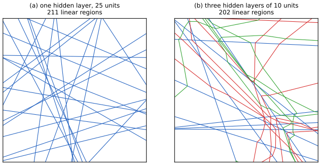
pp. 434–435 An MLP with one hidden layer is a universal approximator: it can approximate any continuous function on a compact set to any accuracy, given enough hidden units (Hornik et al., 1989; Cybenko, 1989; Hornik, 1991). Intuitively each hidden unit specifies a half-plane and enough of them carve up space finely enough to assign any response; Figure 13.7 shows the pieces for ReLU units. Yet deep networks work better than shallow ones in practice and in theory (Montufar et al., 2014; Telgarsky, 2016): later layers reuse the features of earlier ones, so a compositional function (the book's example is the DNA pattern *AA??CGCG??AA*, found by first detecting the motifs AA and CG) is cheaper to represent in depth. Both statements are made precise below.
Filling the gap 13.3: universal approximation, with a rate in one dimension p. 434, [HSW89; Cyb89; Hor91]
Derivation
Statement. Let \(K\subset\R^d\) be compact and \(\varphi:\R\to\R\) continuous with \(\varphi(t)\to0\) as \(t\to-\infty\) and \(\varphi(t)\to1\) as \(t\to+\infty\) (a sigmoidal function: the logistic function and \(\frac12(1+\tanh)\) qualify). Then the set \(S\) of finite sums \(g(\bm x)=\sum_{j=1}^Mc_j\,\varphi(\bm w_j^\T\bm x+b_j)\) is dense in \(C(K)\) for the sup norm. (Leshno et al. (1993) show that continuity and non-polynomiality of \(\varphi\) already suffice; the argument below is Cybenko's.)
Proof. Suppose \(\overline S\ne C(K)\). By the Hahn–Banach theorem there is a nonzero bounded linear functional on \(C(K)\) vanishing on \(\overline S\), and by the Riesz representation theorem it is \(f\mapsto\int f\,\d\mu\) for a nonzero finite signed Borel measure \(\mu\) on \(K\). So \[ \int_K\varphi(\bm w^\T\bm x+b)\,\d\mu(\bm x)=0\qquad\text{for all }\bm w\in\R^d,\ b\in\R. \tag{*} \] Step 1: half-spaces. Fix \(\bm w,b,\theta\) and apply (*) to \((\lambda\bm w,\lambda b+\theta)\): \(\varphi(\lambda(\bm w^\T\bm x+b)+\theta)\) tends, as \(\lambda\to\infty\), to 1 on the open half-space \(\{\bm w^\T\bm x+b>0\}\), to 0 on \(\{\bm w^\T\bm x+b<0\}\) and equals \(\varphi(\theta)\) on the hyperplane \(\{\bm w^\T\bm x+b=0\}\). The functions are bounded (by \(\sup|\varphi|\)), so dominated convergence gives \(\mu(\text{open half-space})+\varphi(\theta)\mu(\text{hyperplane})=0\) for every \(\theta\). Let \(\theta\to-\infty\): \(\mu(\text{open half-space})=0\); then \(\varphi(\theta)\mu(\text{hyperplane})=0\) for all \(\theta\) gives \(\mu(\text{hyperplane})=0\) (take \(\theta\) with \(\varphi(\theta)\ne0\)). Hence \(\mu\) vanishes on every closed half-space too.
Step 2: one-dimensional marginals. Fix \(\bm w\) and let \(\nu\) be the image of \(\mu\) under \(\bm x\mapsto\bm w^\T\bm x\), a finite signed measure on \(\R\) supported in a bounded interval. By Step 1 \(\nu((t,\infty))=0\) and \(\nu(\{t\})=0\) for every \(t\), so \(\nu\) vanishes on all intervals \((s,t]\), a \(\pi\)-system generating the Borel sets, and \(\nu(\R)=0\); hence \(\nu=0\) (a finite signed measure is determined by its values on such a \(\pi\)-system).
Step 3: Fourier transform. Then \(\int e^{i\bm w^\T\bm x}\,\d\mu(\bm x)=\int e^{it}\,\d\nu(t)=0\) for all \(\bm w\): the Fourier transform of the finite measure \(\mu\) vanishes identically, so \(\mu=0\) by uniqueness of the Fourier transform of finite measures. This contradicts \(\mu\ne0\). \(\square\)
ReLU. \(\ReLU(a)-\ReLU(a-1)\) equals 0 for \(a\le0\), \(a\) on \([0,1]\) and 1 for \(a\ge1\): it is continuous and sigmoidal, so linear combinations of ReLU units contain every sigmoidal unit above and the span is dense as well.
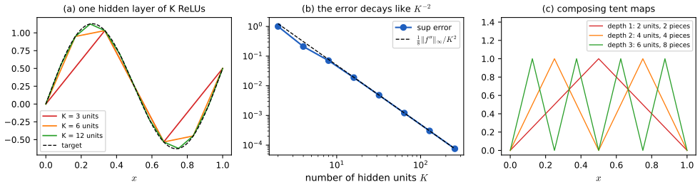
A rate in one dimension. For \(f\in C^2[0,1]\) let \(p_K\) be the piecewise-linear interpolant of \(f\) at the \(K+1\) equally spaced knots \(t_k=k/K\). It is a one-hidden-layer ReLU network with \(K\) units: \(p_K(x)=f(0)+\sum_{k=0}^{K-1}c_k\ReLU(x-t_k)\), where \(c_0\) is the first slope and \(c_k\) the change of slope at \(t_k\). On a cell \([a,b]\) of length \(h=1/K\) let \(e=f-p_K\), which vanishes at \(a\) and \(b\). For \(x\in(a,b)\) put \(g(t)=e(t)-e(x)\frac{(t-a)(t-b)}{(x-a)(x-b)}\); \(g\) has the three zeros \(a,x,b\), so \(g''\) has a zero \(\xi\in(a,b)\) (Rolle twice), i.e. \(e''(\xi)=f''(\xi)=2e(x)/((x-a)(x-b))\). Therefore \[ |f(x)-p_K(x)|=\tfrac12|f''(\xi)|\,(x-a)(b-x)\le\frac{\|f''\|_\infty}{8K^2}. \] So \(K\) units give error \(O(K^{-2})\) for a smooth target (Figure 13.S2a, b: the target \(\sin2\pi x+x/2\) with \(\|f''\|_\infty=4\pi^2\) stays below the bound for \(K\) from 2 to 256). In \(d\) dimensions the analogous bounds degrade like \(K^{-2/d}\) unless the target has special structure: the curse of dimensionality that depth and weight sharing are meant to defeat. \(\square\)
Filling the gap 13.4: depth against width, and the number of linear regions p. 434–435, Figure 13.7
Derivation
Shallow networks in one dimension. A one-hidden-layer ReLU network \(x\mapsto c_0+\sum_{k=1}^mc_k\ReLU(w_kx+b_k)\) is piecewise linear and each unit contributes at most one breakpoint (where \(w_kx+b_k=0\)). So it has at most \(m+1\) linear pieces.
Deep networks reach \(2^L\) pieces with \(2L\) units. On \([0,1]\) the tent map \(T(x)=2\ReLU(x)-4\ReLU(x-\tfrac12)\) equals \(2x\) on \([0,\tfrac12]\) and \(2-2x\) on \([\tfrac12,1]\) and maps \([0,1]\) onto itself. Claim: \(T^{\circ L}\) has \(2^L\) linear pieces, each mapped linearly onto \([0,1]\) (slope \(\pm2^L\)). For \(L=1\) this is the definition. If it holds for \(L-1\), then on each piece \(I\) of \(T^{\circ(L-1)}\) the map sends \(I\) bijectively and linearly onto \([0,1]\), and \(T\) then folds \([0,1]\) once, so \(T^{\circ L}\) restricted to \(I\) has two linear pieces, each mapping onto \([0,1]\). This gives \(2\cdot2^{L-1}\) pieces. As a network, \(T^{\circ L}\) is \(L\) hidden layers of two units, \(2L\) units in all, but a one-hidden-layer network with \(m\) units has at most \(m+1\) pieces, so it needs \(m\ge2^L-1\) units for the same function: exponentially many. (The sawtooth of \(2^L\) teeth in Figure 13.S2c is also what a function that oscillates fast would look like: such targets are cheap in depth and expensive in width.) The same fold-and-compose idea underlies Telgarsky (2016) and Montufar et al. (2014).
Counting regions in the plane. A one-hidden-layer ReLU network on \(\R^2\) is linear on each cell of the arrangement of the \(m\) lines \(\{\bm w_k^\T\bm x+b_k=0\}\), since inside a cell the on/off pattern of every unit is constant. Suppose the lines are in general position (no two parallel, no three through a point). Adding line number \(k\) to an arrangement of \(k-1\) lines: the new line is cut by the old ones at \(k-1\) distinct points into \(k\) pieces, and each piece splits one existing region into two, so \(k\) new regions appear. Hence the number of regions is \(1+\sum_{k=1}^mk=1+m+\binom m2\). For \(m=25\) this is 326. (In \(\R^d\) the same argument gives the recurrence \(R(m,d)=R(m-1,d)+R(m-1,d-1)\) and so \(R(m,d)=\sum_{j=0}^d\binom mj\).) A linear-programming count in the code confirms 37 regions for 8 random lines.
The window of Figure 13.7(a) (25 random lines through a square) meets 211 of the 326 regions; the deeper net of Figure 13.7(b), with only 30 units in three layers, meets 202, and its boundaries bend because the second-layer units are piecewise-linear functions of the first. With depth the number of regions can grow exponentially with the number of layers for suitable weights (Montufar et al., 2014), but for random weights the count is far below the maximum, as here. \(\square\)
13.2.6 The "deep learning revolution"
pp. 435–436 The ideas behind DNNs are decades old; they became widely used in the 2010s, first in speech recognition (Dahl et al., 2011; Hinton et al., 2012) and then, decisively, in image classification, when Krizhevsky, Sutskever and Hinton (2012) cut the ImageNet error from 26 to 16 percent in a year, against a previous rate of about two points per year. Contributing factors: cheap GPUs, large labelled data sets (ImageNet has 1.3 million images), and open-source libraries with automatic differentiation (TensorFlow, PyTorch, MXNet), Section 13.3.
13.2.7 Connections with biology
pp. 436–438 The McCulloch–Pitts neuron (1943), \(h_k(\bm x)=\Heav(\bm w_k^\T\bm x-b_k)\), is the ancestor of the artificial neuron. Artificial networks differ from brains in several ways: backpropagation sends information backwards along an axon, which real neurons cannot do (they use local update rules); brains have many feedback connections (which may implement a prior combined with bottom-up likelihoods); real neurons have complex dendritic trees; artificial networks are (still) smaller; and brains consist of specialised interacting modules rather than one function. Whether such low-level detail matters for intelligence is open; the book's working assumption is that any intelligent agent should follow the principles of information processing and Bayesian decision theory (Section 5.1), with computational shortcuts where the exact answer is intractable.
13.3 Backpropagation
pp. 438–446 (This section of the book is coauthored with Mathieu Blondel.) Backpropagation computes the gradient of a scalar loss, applied to the output of a network, with respect to the parameters of every layer, which a gradient-based optimiser (Section 13.4, Chapter 8) then uses. It was found by Bryson and Ho (1969) and Werbos (1974) and brought to the mainstream by Rumelhart, Hinton and Williams (1986). For a chain of layers it is a repeated application of the chain rule; for an arbitrary directed acyclic graph it is called automatic differentiation (autodiff).
See also: Bayesian and Probabilistic ML, Section 5.3 (error backpropagation) and its backpropagation demo; Foundations of Deep Learning, Section 8.2 (automatic differentiation) and its forward and reverse mode demo; Elements of Statistical Learning, Section 11.4.
13.3.1 Forward vs reverse mode differentiation
pp. 438–440 Let \(\bm o=f(\bm x)\), \(\bm x\in\R^n\), \(\bm o\in\R^m\), with \(f=f_K\circ\cdots\circ f_1\) a chain (13.22), intermediate values \(\bm x_{k+1}=f_k(\bm x_k)\), \(\bm x_1=\bm x\), and layer Jacobians \(\bm J_{f_k}(\bm x_k)\in\R^{m_k\times m_{k-1}}\) (\(m_0=n\), \(m_K=m\)). The chain rule gives (13.23)–(13.24) \[ \bm J_f(\bm x)=\bm J_{f_K}(\bm x_K)\cdots\bm J_{f_2}(\bm x_2)\bm J_{f_1}(\bm x_1). \] The \(j\)-th column of \(\bm J_f\) is a Jacobian-vector product (JVP) \(\bm J_f\bm e_j\); the \(i\)-th row is a vector-Jacobian product (VJP) \(\bm e_i^\T\bm J_f\) (13.25). Forward mode (Algorithm 13.1) evaluates the JVPs by multiplying the product from the right, \(\bm J_{f_K}(\cdots(\bm J_{f_1}\bm v))\), carrying a tangent \(\bm v\) alongside the values, one pass per input direction: \(n\) passes for the full Jacobian. Reverse mode (Algorithm 13.2) first computes and stores all \(\bm x_k\) in a forward pass and then multiplies from the left, \(((\bm u^\T\bm J_{f_K})\bm J_{f_{K-1}})\cdots\), one backward pass per output: \(m\) passes. So forward mode is cheaper when \(n<m\) and reverse mode when \(n>m\); for a loss function (\(m=1\)) and millions of parameters reverse mode is the only choice.
Algorithm 13.1 (forward-mode differentiation) p. 440
- \(\bm x_1:=\bm x\); \(\bm v_j:=\bm e_j\in\R^n\) for \(j=1:n\).
- For \(k=1:K\): \(\bm x_{k+1}=f_k(\bm x_k)\); \(\bm v_j:=\bm J_{f_k}(\bm x_k)\bm v_j\) for \(j=1:n\).
- Return \(\bm o=\bm x_{K+1}\) and the columns \([\bm J_f(\bm x)]_{:,j}=\bm v_j\).
Algorithm 13.2 (reverse-mode differentiation) p. 440
- \(\bm x_1:=\bm x\); for \(k=1:K\): \(\bm x_{k+1}=f_k(\bm x_k)\) (forward pass, storing every \(\bm x_k\)).
- \(\bm u_i:=\bm e_i\in\R^m\) for \(i=1:m\).
- For \(k=K:1\): \(\bm u_i^\T:=\bm u_i^\T\bm J_{f_k}(\bm x_k)\) for \(i=1:m\).
- Return \(\bm o=\bm x_{K+1}\) and the rows \([\bm J_f(\bm x)]_{i,:}=\bm u_i^\T\).
Filling the gap 13.5: what forward and reverse mode cost p. 439–440, below (13.26) and (13.27)
Derivation
Count. Multiplying a dense \(a\times b\) matrix by a vector costs \(ab\) multiply-adds. Let \(S=\sum_{k=1}^Km_km_{k-1}\), the cost of pushing one vector through all the layer Jacobians (the layer Jacobians themselves are taken as given, as in the book). One JVP is a right-to-left sweep and costs \(S\); one VJP is a left-to-right sweep and costs \(S\). Hence the full Jacobian costs \(nS\) by forward mode and \(mS\) by reverse mode (reverse mode also needs the forward pass, a further cost of the same order as \(S\), plus the memory for the stored \(\bm x_k\); forward mode needs no storage). The cheaper mode is the one with the smaller of \(n\) and \(m\).
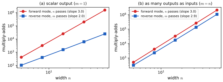
The book's operation count is off by a factor \(n\) for forward mode. The book takes \(m=1\) and \(n=m_1=m_2=m_3\) and states that the cost is \(O(n^2)\) for both modes. With \(m_k=n\) for \(k<K\) and \(m=1\), \(S=(K-1)n^2+n=\Theta(n^2)\), so one pass costs \(\Theta(n^2)\), and forward mode needs \(n\) passes: \(nS=\Theta(n^3)\), whereas reverse mode needs one: \(S=\Theta(n^2)\). (\(O(n^2)\) is the cost of one forward-mode pass, not of the whole Jacobian.) I confirmed this by counting multiply-adds in code for a four-layer tanh chain, with an \(n\times n\) first three layers and a \(1\times n\) last one, \(n=8,16,32,64\): the counts are exactly \(2nS\) (a tangent and a value update per layer) for forward mode and \((1+m)S\) for reverse mode, and the log-log slopes are 2.98 and 1.98. Figure 13.S7a shows this, and 13.S7b the case \(m=n\), where both modes cost \(\Theta(n^3)\).
Which order is best? Multiplying the Jacobians in an arbitrary order is the matrix-chain problem, and forward and reverse mode are its two extreme orders (all products with the vector at the right, or at the left). Choosing the optimal bracketing for a general computation graph is NP-hard (Naumann, 2008), but for \(m=1\) or \(n=1\) the extreme order is optimal, which is why the two modes are all one needs in machine learning. \(\square\)
13.3.2 Reverse mode differentiation for multilayer perceptrons
pp. 440–441 In an MLP each layer \(f_k(\bm x_k,\bm\theta_k)\) also has parameters, and the last layer is a scalar loss \(L\), e.g. for \(\ell_2\) loss with one hidden layer \(L=\tfrac12\|\bm y-\bm W_2\varphi(\bm W_1\bm x)\|^2\) (13.28)–(13.33). Reverse mode starts from the easy gradient \(\partial L/\partial\bm x_4\) and, by the chain rule, obtains (13.34)–(13.36) \[ \frac{\partial L}{\partial\bm\theta_3}=\frac{\partial L}{\partial\bm x_4}\frac{\partial\bm x_4}{\partial\bm\theta_3},\quad \frac{\partial L}{\partial\bm\theta_2}=\frac{\partial L}{\partial\bm x_4}\frac{\partial\bm x_4}{\partial\bm x_3}\frac{\partial\bm x_3}{\partial\bm\theta_2},\ \dots \] recursively: the gradient row vector at layer \(k\) is the one at layer \(k+1\) multiplied by the Jacobian \(\partial\bm x_{k+1}/\partial\bm x_k\) (Algorithm 13.3). The output also includes \(\nabla_{\bm x}L\), not needed for learning but useful for generating inputs (Section 14.6).
Algorithm 13.3 (backpropagation for an MLP with \(K\) layers) p. 442
- Forward pass. \(\bm x_1:=\bm x\); for \(k=1:K\): \(\bm x_{k+1}=f_k(\bm x_k,\bm\theta_k)\).
- Backward pass. \(\bm u_{K+1}:=1\); for \(k=K:1\): \(\bm g_k:=\bm u_{k+1}^\T\,\partial f_k(\bm x_k,\bm\theta_k)/\partial\bm\theta_k\); \(\bm u_k^\T:=\bm u_{k+1}^\T\,\partial f_k(\bm x_k,\bm\theta_k)/\partial\bm x_k\).
- Return \(L=\bm x_{K+1}\), \(\nabla_{\bm x}L=\bm u_1\) and \(\{\nabla_{\bm\theta_k}L=\bm g_k\}\).
13.3.3 Vector-Jacobian product for common layers
pp. 441–444 It remains to say how to compute \(\bm u^\T\bm J_f\) for each layer type; Algorithm 13.3 only ever needs these products, never a full Jacobian.
13.3.3.1 Cross entropy layer. For logits \(\bm x\) and a label distribution \(\bm y\) (often one-hot), \(z=-\sum_cy_c\log\softmax(\bm x)_c=\log\sum_je^{x_j}-\sum_cy_cx_c\) (for \(\sum_cy_c=1\)) has Jacobian \[ \frac{\partial z}{\partial\bm x}=(\bm p-\bm y)^\T,\qquad\bm p=\softmax(\bm x). \tag{13.39} \] 13.3.3.2 Elementwise nonlinearity. For \(z_i=\varphi(x_i)\), \(\bm J=\diag(\varphi'(\bm x))\) (13.42)–(13.43), so \(\bm u^\T\bm J=(\bm u\odot\varphi'(\bm x))^\T\): an elementwise product. For ReLU, \(\varphi'(a)=\Heav(a)\) away from 0 and any value in \([0,1]\) is a subgradient at 0 (usually 0 is used).
13.3.3.3 Linear layer. For \(\bm z=\bm W\bm x\) with \(\bm W\in\R^{m\times n}\): \(\partial\bm z/\partial\bm x=\bm W\) (13.49), so \(\bm u^\T\bm J=\bm u^\T\bm W\) (13.50), and the gradient with respect to the weights is the outer product \(\bm u\bm x^\T\in\R^{m\times n}\) (13.55).
13.3.3.4 Putting it together is Exercise 13.1 (solved below).
Filling the gap 13.6: the backpropagation recursion and the three layer VJPs pp. 441–444, (13.39)–(13.55), (13.73)–(13.78)
Derivation
The recursion. Consider an MLP with \(\bm z_0=\bm x\), \(\bm a_l=\bm W_l\bm z_{l-1}+\bm b_l\), \(\bm z_l=\varphi(\bm a_l)\) for \(l<L\), logits \(\bm a_L\) and loss \(L=\mathrm{CE}(\bm y,\softmax(\bm a_L))\). Define the error signals (column vectors) \(\bm\delta_l=\nabla_{\bm a_l}L\). Then \[ \bm\delta_L=\bm p-\bm y,\qquad\bm\delta_l=(\bm W_{l+1}^\T\bm\delta_{l+1})\odot\varphi'(\bm a_l),\qquad\nabla_{\bm W_l}L=\bm\delta_l\bm z_{l-1}^\T,\quad\nabla_{\bm b_l}L=\bm\delta_l,\quad\nabla_{\bm x}L=\bm W_1^\T\bm\delta_1. \] Proof. \(L\) depends on \(\bm a_l\) only through \(\bm a_{l+1}=\bm W_{l+1}\varphi(\bm a_l)+\bm b_{l+1}\), whose Jacobian with respect to \(\bm a_l\) is \(\bm W_{l+1}\diag(\varphi'(\bm a_l))\). By the chain rule \(\nabla_{\bm a_l}L=\diag(\varphi'(\bm a_l))\bm W_{l+1}^\T\bm\delta_{l+1}\), the stated recursion. The weight and bias gradients follow from \(a_{l,k}=\sum_jW_{l,kj}z_{l-1,j}+b_{l,k}\): \(\partial L/\partial W_{l,kj}=\delta_{l,k}z_{l-1,j}\) and \(\partial L/\partial b_{l,k}=\delta_{l,k}\); the input gradient uses \(\partial a_{1,k}/\partial x_j=W_{1,kj}\). Each layer costs two matrix-vector products (\(\bm W^\T\bm\delta\) and \(\bm\delta\bm z^\T\)) against one for the forward pass, so the backward pass costs about twice the forward pass, and the whole gradient about three times the forward cost.
Cross entropy (13.39)–(13.41). With \(\sum_cy_c=1\), \(z=\log\sum_je^{x_j}-\sum_cy_cx_c\), so \(\partial z/\partial x_i=e^{x_i}/\sum_je^{x_j}-y_i=p_i-y_i\). For label distributions that do not sum to one (e.g. weighted soft labels) the gradient is \((\sum_cy_c)\bm p-\bm y\); the book's (13.38) implicitly assumes \(\sum_cy_c=1\).
Linear layer (13.47)–(13.55). \(z_k=\sum_lW_{kl}x_l\) gives \(\partial z_k/\partial x_j=W_{kj}\) and \(\partial z_k/\partial W_{ij}=\delta_{ki}x_j\) (nonzero only for \(k=i\)). For a given \(\bm u\), \(\sum_ku_k\,\partial z_k/\partial W_{ij}=u_ix_j\), the \((i,j)\) entry of \(\bm u\bm x^\T\).
Shapes in (13.73)–(13.78). For \(\bm z=\sigma(\bm W\bm x)\) the Jacobian is \(\partial\bm z/\partial\bm x=\diag(\bm z\odot(1-\bm z))\bm W\in\R^{m\times n}\) (the book writes \(\diag(\bm z(1-\bm z)^\T)\bm W\), which should be read as \(\diag(\bm z\odot(1-\bm z))\bm W\)). For \(\bm z=\ReLU(\bm W\bm x)\) it is \(\partial\bm z/\partial\bm x=\diag(\ind(\bm z>0))\bm W\), an \(m\times n\) matrix; the printed \(\bm W^\T\ind(\bm z>0)\) in (13.77) has the shape \(n\times m\) and is the transpose that appears when the VJP is written as a gradient: \(\nabla_{\bm x}(\bm u^\T\bm z)=\bm W^\T(\bm u\odot\ind(\bm z>0))\). Likewise the expressions in (13.74) and (13.78), \(\bm z(1-\bm z)\bm x^\T\) and \(\ind(\bm z>0)\bm x^\T\), are the weight gradients for the upstream vector \(\bm u=\bm 1\); in general they are \((\bm u\odot\bm z\odot(1-\bm z))\bm x^\T\) and \((\bm u\odot\ind(\bm z>0))\bm x^\T\). A finite-difference check of all of these, and of the whole recursion against PyTorch's autograd for five activation functions, passes to \(10^{-10}\). \(\square\)
13.3.4 Computation graphs
pp. 444–446 Modern networks combine differentiable components into a directed acyclic graph (DAG): each node is a differentiable function of its parents, with nodes numbered in topological order (parents before children). The book's example is \(f(x_1,x_2)=x_2e^{x_1}\sqrt{x_1+x_2e^{x_1}}\) (13.56), evaluated by \[ x_3=e^{x_1},\quad x_4=x_2x_3,\quad x_5=x_1+x_4,\quad x_6=\sqrt{x_5},\quad x_7=x_4x_6, \tag{13.57–13.61} \] (Figure 13.11, a drawing). Because the graph is not a chain, a node can influence the output along several paths, e.g. \(x_4\) feeds \(x_5\) and \(x_7\), so the backward pass sums over the children (13.62): \[ \frac{\partial o}{\partial x_j}=\sum_{k\in\mathrm{Ch}(j)}\frac{\partial o}{\partial x_k}\frac{\partial x_k}{\partial x_j}, \tag{13.67} \] where \(\partial o/\partial x_k\) (the adjoint of \(k\)) has already been computed, because we work in reverse topological order. The graph can be defined ahead of time (a static graph, TensorFlow 1) or traced while the function runs (JAX, PyTorch, TensorFlow eager), which allows dynamic graphs whose shape depends on the data. Figure 13.13 is the graph of an MLP with weight decay: \(\bm z=\bm W^{(1)}\bm x\), \(\bm h=\varphi(\bm z)\), \(\bm o=\bm W^{(2)}\bm h\), \(L=\ell(\bm o,y)\), \(s=\frac\lambda2(\|\bm W^{(1)}\|_F^2+\|\bm W^{(2)}\|_F^2)\), \(J=L+s\).
At \((x_1,x_2)=(0.7,1.3)\) the forward and backward passes give the following numbers.
| node | \(x_1\) | \(x_2\) | \(x_3\) | \(x_4\) | \(x_5\) | \(x_6\) | \(x_7=f\) |
|---|---|---|---|---|---|---|---|
| value | 0.7000 | 1.3000 | 2.0138 | 2.6179 | 3.3179 | 1.8215 | 4.7685 |
| adjoint \(\partial f/\partial x_j\) | 7.3683 | 5.1151 | 3.3021 | 2.5401 | 0.7186 | 2.6179 | 1 |
The two partial derivatives of \(f\) are the adjoints of the two inputs, obtained in one backward sweep; forward mode needs two sweeps (seed \(x_1\), then \(x_2\)).
Filling the gap 13.7: adjoints on a DAG and the cost of reverse mode pp. 444–446, (13.62)–(13.67)
Derivation
Setup. Nodes \(x_1,\dots,x_N\) are numbered topologically, \(x_k=f_k(x_{\mathrm{Pa}(k)})\) for \(k>n\) (with \(x_1,\dots,x_n\) the inputs) and the output is \(o=x_N\). For each \(j\) define \(\Phi_j(x_1,\dots,x_j)\) as the output obtained by running the nodes \(j+1,\dots,N\) from the first \(j\) values treated as free variables. Then \(\Phi_N=x_N\) and \(\Phi_j(x_1,\dots,x_j)=\Phi_{j+1}(x_1,\dots,x_j,f_{j+1}(x_{\mathrm{Pa}(j+1)}))\). The adjoint is \(\bar x_j:=\partial\Phi_j/\partial x_j\), the partial derivative of the output with respect to the value of node \(j\), holding \(x_1,\dots,x_{j-1}\) fixed and re-running its descendants. (This is the precise meaning of \(\partial o/\partial x_j\) in (13.67): the descendants of \(x_j\) are recomputed, its non-descendants are held fixed.)
Claim. \(\bar x_j=\sum_{k\in\mathrm{Ch}(j)}\bar x_k\,\partial f_k/\partial x_j\). Proof by differentiating the identity above with respect to \(x_i\), \(i\le j\), using the chain rule: for \(i\notin\mathrm{Pa}(j+1)\), \(\partial\Phi_j/\partial x_i=\partial\Phi_{j+1}/\partial x_i\); for \(i\in\mathrm{Pa}(j+1)\), \(\partial\Phi_j/\partial x_i=\partial\Phi_{j+1}/\partial x_i+\bar x_{j+1}\,\partial f_{j+1}/\partial x_i\). Starting from \(\bar x_N=1\) and descending \(k=N,N-1,\dots\), each node \(k\) therefore adds the contribution \(\bar x_k\,\partial f_k/\partial x_i\) to the running adjoint of each of its parents \(i\), and after all \(k>j\) have been processed the running adjoint of \(j\) is \(\sum_{k\in\mathrm{Ch}(j)}\bar x_k\,\partial f_k/\partial x_j=\partial\Phi_j/\partial x_j=\bar x_j\), by induction on \(j\) downwards. The sum over children is precisely what makes the multi-path case correct. At the inputs, \(\bar x_i=\partial f/\partial x_i\).
Cost. The backward update of node \(k\) multiplies its adjoint by the local partials \(\partial f_k/\partial x_i\), a quantity of the same kind as the forward evaluation of \(f_k\): for \(+\) the cost is a copy, for \(\times\) two multiplications against one, for a matrix product two matrix products against one, for \(\exp\) and \(\sqrt{\ }\) a multiplication that reuses the stored forward value. So for the elementary operations of a network the reverse sweep costs at most a small constant times the forward sweep, independent of the number \(n\) of inputs: the gradient of a scalar function costs \(O(1)\) function evaluations. (This is the "cheap gradient principle" of Baur and Strassen (1983); see Griewank and Walther (2008).) The price is memory: all values needed by the local partials (here \(x_3,x_4,x_6\)) must be stored, or recomputed.
Worked example. At \((0.7,1.3)\) the backward sweep gives \(\bar x_7=1\); \(\bar x_6=\bar x_7x_4=2.6179\); \(\bar x_5=\bar x_6\cdot\frac1{2x_6}=0.7186\); \(\bar x_4=\bar x_5\cdot1+\bar x_7x_6=0.7186+1.8215=2.5401\) (two paths); \(\bar x_3=\bar x_4x_2=3.3021\); \(\bar x_2=\bar x_4x_3=5.1151\); \(\bar x_1=\bar x_5\cdot1+\bar x_3x_3=0.7186+6.6497=7.3683\) (two paths). These agree with the closed forms \(\partial f/\partial x_1=x_2e^{x_1}\sqrt{s}+x_2e^{x_1}(1+x_2e^{x_1})/(2\sqrt s)\) and \(\partial f/\partial x_2=e^{x_1}\sqrt s+x_2e^{2x_1}/(2\sqrt s)\), \(s=x_1+x_2e^{x_1}\), with finite differences, and with forward mode with each of the two seeds. \(\square\)
13.4 Training neural networks
pp. 446–454 The standard approach is maximum likelihood: minimise \(L(\bm\theta)=-\log p(\mathcal D\given\bm\theta)=-\sum_{n=1}^N\log p(\bm y_n\given\bm x_n;\bm\theta)\) (13.68), usually with a regulariser (Section 13.5), by passing the gradient from backpropagation to an optimiser of Chapter 8 (Adam, Section 8.4.6.3, is a popular choice: it scales to large data through minibatches and converges fairly fast through momentum and diagonal preconditioning). In practice several things can go wrong. The loss is not convex, so we cannot expect the global optimum, although SGD often finds surprisingly good solutions (Section 13.5.6).
See also: Foundations of Deep Learning, Section 7.2 (gradient descent optimization) and 7.3.3 (RMSProp and Adam); Elements of Statistical Learning, Section 11.5 (some issues in training).
13.4.1 Tuning the learning rate
p. 447 The step size must be tuned to converge to a good solution; see Section 8.4.3 of the book and the step-size experiments of the logistic regression optimiser demo (Chapter 10), where a step above \(2/\lambda_{\max}\) of the Hessian makes gradient descent bounce.
13.4.2 Vanishing and exploding gradients
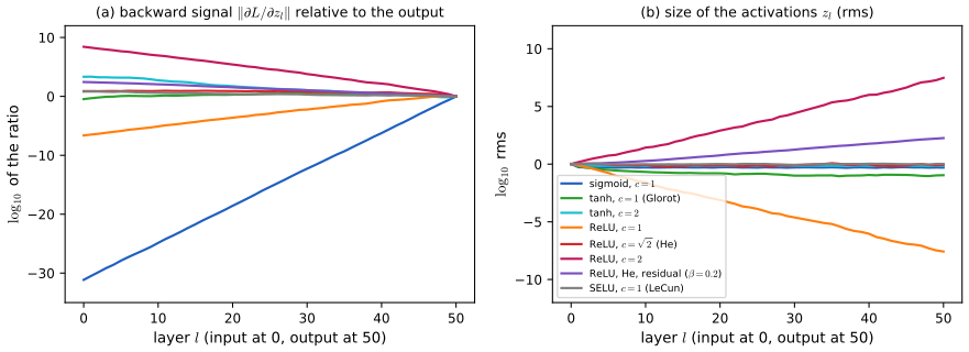
p. 447–448 In a very deep network the gradient tends to become tiny (vanishing) or huge (exploding), because the error signal passes through many layers. For the gradient with respect to the activations of layer \(l\), \[ \frac{\partial L}{\partial\bm z_l}=\bm J_l\bm g_{l+1},\qquad\bm J_l=\frac{\partial\bm z_{l+1}}{\partial\bm z_l},\quad\bm g_{l+1}=\frac{\partial L}{\partial\bm z_{l+1}}, \tag{13.69} \] (as a column vector this is \(\bm J_l^\T\bm g_{l+1}\); see the notes on the book) and if \(\bm J_l=\bm J\) is the same for all layers the gradient arriving from the top is \(\bm J^{L-l}\bm g_L\) in the book's notation. Its behaviour is governed by the spectral radius \(\lambda\) of \(\bm J\): above 1 the gradient can explode, below 1 it can vanish. Gradient clipping cures explosion by capping the norm, \(\bm g'=\min(1,c/\|\bm g\|)\,\bm g\) (13.70). Vanishing is harder; the solutions listed in the book are: change the activation function (13.4.3), add additive skip paths (13.4.4), standardise activations (batch normalisation, Section 14.2.4.1) and initialise carefully (13.4.5).
Filling the gap 13.8: why gradients vanish or explode, bounds, and gradient clipping pp. 447–448, (13.69), (13.70)
Derivation
The product of Jacobians. With \(\bm z_{l+1}=f_l(\bm z_l)\), the chain rule for the gradient with respect to \(\bm z_l\) is \(\bm g_l=\bm J_l^\T\bm g_{l+1}\), so \(\bm g_l=\bm J_l^\T\bm J_{l+1}^\T\cdots\bm J_{L-1}^\T\bm g_L\). (The book's (13.69) writes \(\bm J_l\bm g_{l+1}\), which is the row-vector convention \(\bm g_l^\T=\bm g_{l+1}^\T\bm J_l\); the conclusions are unaffected because \(\bm J\) and \(\bm J^\T\) have the same eigenvalues and singular values.)
Bound. By submultiplicativity of the spectral norm, \(\|\bm g_l\|\le\prod_{j=l}^{L-1}\|\bm J_j\|_2\,\|\bm g_L\|\). For a sigmoid layer \(\bm z_{j+1}=\sigma(\bm W_{j+1}\bm z_j)\) the Jacobian is \(\diag(\bm z_{j+1}\odot(1-\bm z_{j+1}))\bm W_{j+1}\) and every diagonal entry is at most \(\frac14\) (gap 13.9), so \(\|\bm J_j\|_2\le\frac14\|\bm W_{j+1}\|_2\). Hence \[ \|\bm g_l\|\le\prod_{j}\frac{\|\bm W_{j+1}\|_2}{4}\ \|\bm g_L\|, \] which decays geometrically with depth whenever \(\|\bm W_j\|_2<4\). For a \(64\times64\) matrix with independent \(\N(0,c^2/64)\) entries the largest singular value is close to \(2c\) (the edge of the quarter-circle law), so for \(c=1\) the bound gives a factor of at most 0.5 per layer. Measured in the demonstration, a 50-layer sigmoid network has \(\|\bm g_0\|/\|\bm g_{50}\|=7\times10^{-32}\): a factor \(0.24\) per layer, within the bound.
Constant Jacobian: spectral radius. If \(\bm J\) is the same for all layers, \(\bm g_l=(\bm J^\T)^{L-l}\bm g_L\). By Gelfand's formula \(\|\bm A^k\|^{1/k}\to\rho(\bm A)\) for any matrix \(\bm A\) and any norm, with \(\rho\) the spectral radius, and \(\rho(\bm J^\T)=\rho(\bm J)\). If \(\rho<1\), then for every \(\epsilon>0\) with \(\rho+\epsilon<1\) there is \(C\) with \(\|(\bm J^\T)^k\|\le C(\rho+\epsilon)^k\to0\): the gradient vanishes geometrically for every starting vector. If \(\rho>1\), then \(\|(\bm J^\T)^k\|\ge\rho^k\) (since \(\rho(\bm A)^k=\rho(\bm A^k)\le\|\bm A^k\|\)), and for a starting vector with a nonzero component along the dominant eigenvector (almost every vector) the norm of \((\bm J^\T)^k\bm g\) grows like \(\rho^k\): the gradient explodes. Complex eigenvalues add rotation but not growth. The case \(\rho=1\) is marginal. For nonconstant Jacobians the same picture holds with the geometric mean of the Jacobian norms in place of \(\rho\).
Clipping. Let \(\bm g'=\min(1,c/\|\bm g\|)\bm g\). If \(\|\bm g\|\le c\) then \(\bm g'=\bm g\); otherwise \(\bm g'=(c/\|\bm g\|)\bm g\) has norm exactly \(c\). So \(\|\bm g'\|\le c\) always, and since the factor is a positive scalar, \(\bm g'\) points in the same direction as \(\bm g\) and is still a descent direction. \(\square\)
13.4.3 Non-saturating activation functions
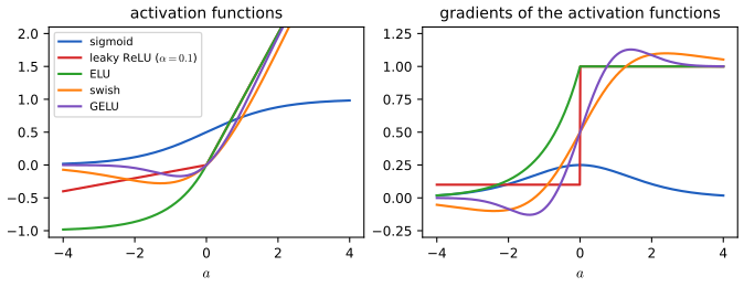
pp. 448–451 For \(\bm z=\sigma(\bm W\bm x)\) the derivative \(\varphi'(a)=\sigma(a)(1-\sigma(a))\) (13.72) is close to 0 when \(\bm z\) is near 0 or 1; the Jacobians with respect to inputs and weights are \(\diag(\bm z\odot(1-\bm z))\bm W\) and (for upstream \(\bm u\)) \((\bm u\odot\bm z\odot(1-\bm z))\bm x^\T\) (13.73, 13.74), so a saturated unit passes no gradient. Large initial weights make saturation likely. Table 13.4 lists the alternatives:
| name | definition | range |
|---|---|---|
| sigmoid | \(\sigma(a)=1/(1+e^{-a})\) | \([0,1]\) |
| tanh | \(2\sigma(2a)-1\) | \([-1,1]\) |
| softplus | \(\log(1+e^a)\) | \([0,\infty)\) |
| ReLU | \(\max(a,0)\) | \([0,\infty)\) |
| leaky ReLU | \(\max(a,0)+\alpha\min(a,0)\) | \(\R\) |
| ELU | \(\max(a,0)+\min(\alpha(e^a-1),0)\) | \([-\alpha,\infty)\) |
| swish | \(a\,\sigma(a)\) | \([-0.28,\infty)\) |
| GELU | \(a\,\Phi(a)\) | \([-0.17,\infty)\) |
13.4.3.1 ReLU. \(\ReLU'(a)=\ind(a>0)\) (13.76); for \(\bm z=\ReLU(\bm W\bm x)\) the gradients are \(\bm W^\T(\bm u\odot\ind(\bm z>0))\) and \((\bm u\odot\ind(\bm z>0))\bm x^\T\) (13.77, 13.78 in corrected form), nonzero as long as the unit is active. A unit that is negative on all the data gets zero gradient forever: a dead ReLU (Lu et al., 2019).
13.4.3.2 Non-saturating ReLUs. The leaky ReLU \(\max(\alpha a,a)\), \(0<\alpha<1\) (13.79), keeps a slope \(\alpha\) on negative inputs (the parametric ReLU learns \(\alpha\)). The ELU (13.80) is smooth: \(\alpha(e^a-1)\) for \(a\le0\), \(a\) otherwise; its first derivative is continuous only if \(\alpha=1\) (footnote 6). The SELU \(\lambda\,\mathrm{ELU}(a;\alpha)\) (13.81) with specific \(\alpha\approx1.6733\) and \(\lambda\approx1.0507\) keeps standardised inputs standardised (Klambauer et al., 2017).
13.4.3.3 Other choices. Swish \(a\,\sigma(\beta a)\) (13.82), found by black-box search (Ramachandran et al., 2017) and also called SiLU, and the GELU \(a\Phi(a)\) (13.83)–(13.84), a "soft ReLU" that replaces the step \(\ind(a>0)\) by the Gaussian cdf. It is the expectation of a stochastic gate: with \(m\sim\mathrm{Ber}(\Phi(a))\), \(\E[am]=a\Phi(a)\) (13.85), an adaptive version of dropout. It is not convex or monotone, and \(\mathrm{GELU}(a)\approx a\sigma(1.702a)\) (13.86).
Filling the gap 13.9: facts about the activation functions, dead ReLUs and the SELU constants pp. 448–451, (13.72)–(13.86)
Derivation
Sigmoid and tanh. \(\sigma'=\sigma(1-\sigma)\) (13.72): differentiate \(\sigma=(1+e^{-a})^{-1}\) to get \(e^{-a}/(1+e^{-a})^2=\sigma\cdot(1-\sigma)\). With \(t=\sigma(a)\in(0,1)\), \(t(1-t)\le\frac14\) (AM–GM), with equality at \(a=0\). From \(\tanh a=2\sigma(2a)-1\): \(\tanh'(a)=4\sigma'(2a)=1-\tanh^2a\le1\), equal to 1 only at 0, and the derivative decays like \(4e^{-2|a|}\).
Dead ReLU. Let unit \(k\) of a first hidden layer have \(a_{kn}=\bm w_k^\T\bm x_n+b_k<0\) for every training input \(\bm x_n\). Then \(\ReLU'(a_{kn})=0\) for all \(n\), so by the recursion of gap 13.6 its error signal \(\delta_{kn}=0\) and \(\nabla_{\bm w_k}L=\sum_n\delta_{kn}\bm x_n=\bm 0\), \(\partial L/\partial b_k=0\) for any loss. A gradient step leaves \((\bm w_k,b_k)\) unchanged, so the unit stays dead forever (with weight decay its parameters shrink towards 0 but it stays off). In deeper layers the unit can be revived indirectly, because earlier layers still move and change its input. The leaky ReLU, whose derivative is \(\alpha>0\) on the negative side, avoids this. The code verifies that an artificially killed unit has exactly zero gradient.
ELU. For \(\alpha(e^a-1)\) (\(a\le0\)) the derivative at \(0^-\) is \(\alpha e^0=\alpha\); for \(a>0\) it is 1. The two agree iff \(\alpha=1\); the function itself is continuous for every \(\alpha\) since \(\alpha(e^0-1)=0\).
GELU, swish. \(\E[a\,m]=a\Pr(m=1)=a\Phi(a)\) for \(m\sim\mathrm{Ber}(\Phi(a))\) (13.85). The logistic cdf \(\sigma(1.702a)\) is within 0.0095 of \(\Phi(a)\) for all \(a\) (numerically: maximum difference 0.00949), so \(\mathrm{GELU}(a)=a\Phi(a)\) differs from \(a\sigma(1.702a)\) by at most \(0.0203\) over \([-8,8]\) (13.86). As \(\beta\to\infty\), \(a\sigma(\beta a)\to a\ind(a>0)=\ReLU(a)\), so swish interpolates between \(a/2\) (\(\beta=0\)) and ReLU. The minimum value of swish with \(\beta=1\) is \(-0.278\) at \(a\approx-1.28\), of GELU \(-0.170\) at \(a\approx-0.75\), hence the ranges in Table 13.4.
The SELU constants. Let \(z\sim\N(0,1)\) and \(\mathrm{SELU}(z)=\lambda z\) for \(z>0\), \(\lambda\alpha(e^z-1)\) for \(z\le0\). Use \(\E[z\ind(z>0)]=1/\sqrt{2\pi}\), \(\E[z^2\ind(z>0)]=\frac12\) and \(\E[e^{kz}\ind(z\le0)]=e^{k^2/2}\Phi(-k)\). Then \[ \E[\mathrm{SELU}(z)]=\lambda\Big[\tfrac1{\sqrt{2\pi}}+\alpha\big(\sqrt e\,\Phi(-1)-\tfrac12\big)\Big],\quad \E[\mathrm{SELU}(z)^2]=\lambda^2\Big[\tfrac12+\alpha^2\big(e^2\Phi(-2)-2\sqrt e\,\Phi(-1)+\tfrac12\big)\Big]. \] Setting the first to 0 gives \(\alpha=\dfrac{1/\sqrt{2\pi}}{\frac12-\sqrt e\,\Phi(-1)}=1.6733\ldots\) and then the second to 1 gives \(\lambda=1.0507\ldots\): these are the book's constants (numerically, with these values the mean is \(10^{-16}\) and the second moment \(1.000000\)). So \(\N(0,1)\) is a fixed point of the map "pass a Gaussian through SELU, then recompute mean and variance". The stronger claim of Klambauer et al. (2017), that the fixed point is attracting for layers whose weights have \(\sum_jw_{ij}=0\) and \(\sum_jw_{ij}^2=1\), needs their theorem; I confirm it numerically: starting the variance at 0.1, 0.5, 3 and 8, iterating the one-layer variance map for 150 layers converges to \(1\pm10^{-4}\). (Convergence is slow, tens of layers.) \(\square\)
13.4.4 Residual connections
pp. 451–452 A residual network (He et al., 2016) uses blocks \(F_l'(\bm x)=F_l(\bm x)+\bm x\) (13.87), where \(F_l\) is a shallow nonlinear map (linear-activation-linear). The block computes the "delta" to add to the input. The parameter count is unchanged, but training is easier because the gradient flows directly from the output to earlier layers (Figure 13.15, a drawing). Telescoping gives the activations at the output in terms of any earlier layer \(l\): \[ \bm z_L=\bm z_l+\sum_{i=l}^{L-1}F_i(\bm z_i;\bm\theta_i), \tag{13.88} \] and hence, for the gradient with respect to the parameters of layer \(l\) (13.89)–(13.92), \[ \frac{\partial L}{\partial\bm\theta_l}=\frac{\partial\bm z_l}{\partial\bm\theta_l}\frac{\partial L}{\partial\bm z_L}\Big(\bm I+\sum_{i=l}^{L-1}\frac{\partial F_i(\bm z_i;\bm\theta_i)}{\partial\bm z_l}\Big)=\frac{\partial\bm z_l}{\partial\bm z_l}\frac{\partial L}{\partial\bm z_L}+\text{other terms}: \] the gradient at layer \(l\) contains \(\partial L/\partial\bm z_L\) directly, independently of depth.
Filling the gap 13.10: residual connections and the identity path pp. 451–452, (13.87)–(13.92)
Derivation
Telescoping (13.88). \(\bm z_{i+1}=\bm z_i+F_i(\bm z_i)\) for each \(i\); summing from \(i=l\) to \(L-1\) cancels the intermediate terms.
The Jacobian is a product of \((\bm I+\bm J_i)\). Let \(\bm J_i=\partial F_i(\bm z_i)/\partial\bm z_i\) be the local Jacobian. Then \(\partial\bm z_{i+1}/\partial\bm z_i=\bm I+\bm J_i\), so \[ \frac{\partial\bm z_L}{\partial\bm z_l}=(\bm I+\bm J_{L-1})\cdots(\bm I+\bm J_l)=\bm I+\sum_i\bm J_i+\sum_{i>j}\bm J_i\bm J_j+\cdots. \] Differentiating (13.88) directly gives \(\partial\bm z_L/\partial\bm z_l=\bm I+\sum_{i}\mathrm{d}F_i(\bm z_i)/\mathrm{d}\bm z_l\) with total derivatives, since \(\bm z_i\) itself depends on \(\bm z_l\); the book's (13.91) is correct only with this reading (\(\partial F_i/\partial\bm z_l\) meaning the total derivative through all intermediate layers). Both expansions are the same matrix; the code checks this numerically on a 6-block residual chain.
Depth-independent gradient. The gradient of the loss with respect to \(\bm z_l\) is \(\bm g_l=\big(\prod_i(\bm I+\bm J_i)\big)^\T\bm g_L\), which contains \(\bm g_L\) itself (the "\(\bm I\)" term). Quantitatively, if \(\sum_{i=l}^{L-1}\|\bm J_i\|_2\le s\), then \(\|\prod_i(\bm I+\bm J_i)-\bm I\|_2\le\prod_i(1+\|\bm J_i\|_2)-1\le e^s-1\) (expand the product and use \(1+t\le e^t\)), hence \[ \|\bm g_l-\bm g_L\|\le(e^s-1)\|\bm g_L\|. \] For \(s\) small the gradient at layer \(l\) equals the gradient at the output up to a small relative error, however many layers lie in between: the contrast with the plain network, where \(\bm g_l=\bm J_l^\T\cdots\bm J_{L-1}^\T\bm g_L\) is a product of factors that can all be smaller than 1. The gradient of the weights follows by multiplying with \(\partial\bm z_l/\partial\bm\theta_l\).
Caveat. The forward signal can grow. With \(\bm z_{l+1}=\bm z_l+\beta\varphi(\bm W\bm z_l)\) the second moment of \(\bm z_{l+1}\) is that of \(\bm z_l\) plus \(\beta^2\) times that of the branch plus a cross term \(2\beta\E[\bm z_l^\T\varphi(\bm W\bm z_l)]\) (which vanishes for the first block, where \(\bm z_l\) is symmetric, but is positive afterwards because the ReLU branch output is positively correlated with its input), so it grows geometrically, faster the larger \(\beta\) is. In the demonstration with \(\beta=0.2\) over 50 layers the backward signal at layer 0 is 274 times the output gradient (against \(10^{-31}\) for the sigmoid network) and the activations grow to rms 181, about 1.23 per layer in the second moment. Practical residual networks therefore scale the branch down or normalise it (Section 14.2.4.1). \(\square\)
13.4.5 Parameter initialization
pp. 452–453 The loss is not convex, so the initial weights influence which solution is found and how well information flows forwards and backwards.
13.4.5.1 Heuristic schemes. Glorot and Bengio (2010) observed that weights drawn from \(\N(0,\sigma^2)\) with fixed \(\sigma\) can make activations or gradients blow up. For a linear unit \(o_i=\sum_{j=1}^{n_{\rm in}}w_{ij}x_j\) with independent \(w_{ij}\sim\N(0,\sigma^2)\), \(\E[x_j]=0\), \(\V[x_j]=\gamma^2\), the mean and variance of the output are \(0\) and \(n_{\rm in}\sigma^2\gamma^2\) (13.93)–(13.94). Keeping the variance constant needs \(n_{\rm in}\sigma^2=1\); by the same reasoning for the backward pass, \(n_{\rm out}\sigma^2=1\). The compromise \[ \sigma^2=\frac2{n_{\rm in}+n_{\rm out}} \tag{13.95} \] is Xavier or Glorot initialisation; \(\sigma^2=1/n_{\rm in}\) is LeCun's and \(\sigma^2=2/n_{\rm in}\) is He's (He et al., 2015). Only the first two moments were used, so a uniform distribution works equally well, \(w_{ij}\sim\mathrm{Unif}(-a,a)\) with \(a=\sqrt{6/(n_{\rm in}+n_{\rm out})}\) since the variance is \(a^2/3\). Recommendations: Glorot for linear, tanh, logistic and softmax units; He for ReLU and variants; LeCun for SELU.
13.4.5.2 Data-driven schemes. Layer-sequential unit-variance (LSUV) initialisation (Mishkin and Matas, 2016) starts from orthonormal matrices (Saxe et al., 2014; a Gaussian matrix followed by a QR or SVD) and rescales each layer, \(\bm W_l\leftarrow\bm W_l/\sqrt{v_l}\), where \(v_l\) is the variance of the layer's activations on one minibatch; it is orthogonal initialisation plus batch normalisation applied once.
See also: Foundations of Deep Learning, Section 7.2.5 (parameter initialization) and its initialization and depth demo; Elements of Statistical Learning, Section 11.5.1 (starting values).
Filling the gap 13.11: variance-preserving initialisation pp. 452–453, (13.93)–(13.95)
Derivation
Forward variance (13.93)–(13.94). Let \(o_i=\sum_jw_{ij}x_j\) with \(w_{ij}\) independent of the \(x_j\) and of each other, \(\E w_{ij}=0\), \(\V w_{ij}=\sigma^2\), \(\E x_j=0\), \(\V x_j=\gamma^2\). Then \(\E o_i=\sum_j\E w_{ij}\E x_j=0\) and \(\E o_i^2=\sum_{j,k}\E[w_{ij}w_{ik}]\E[x_jx_k]=\sum_j\sigma^2\E x_j^2=n_{\rm in}\sigma^2\gamma^2\) (the cross terms \(j\ne k\) vanish because \(\E[w_{ij}w_{ik}]=0\)); this uses only the first two moments, not Gaussianity. I confirmed the ratio 1.006 against \(n_{\rm in}\sigma^2\gamma^2\) with \(n_{\rm in}=200\) and \(4\cdot10^5\) samples.
Backward variance. For a linear layer \(\bm o=\bm W\bm x\) the gradient with respect to the input is \(\bm W^\T\bm\delta\), whose \(j\)-th entry is \(\sum_iw_{ij}\delta_i\) with \(n_{\rm out}\) terms: variance \(n_{\rm out}\sigma^2\V\delta\). Hence the condition \(n_{\rm out}\sigma^2=1\). The two conditions \(\sigma^2=1/n_{\rm in}\) and \(\sigma^2=1/n_{\rm out}\) agree if \(n_{\rm in}=n_{\rm out}\); otherwise \(\sigma^2=2/(n_{\rm in}+n_{\rm out})\) is the harmonic mean of the two, (13.95). A uniform law on \((-a,a)\) has variance \(a^2/3\), so \(a=\sqrt{3\sigma^2}=\sqrt{6/(n_{\rm in}+n_{\rm out})}\).
Why ReLU needs the factor 2. If a pre-activation \(a\) is symmetric about 0 then \(\E[\ReLU(a)^2]=\E[a^2\ind(a>0)]=\frac12\E a^2\). Writing \(m_l=\E z_{l}^2\) for the second moment of an activation, a ReLU layer with weight variance \(\sigma^2\) gives \(m_l=\tfrac12n_{\rm in}\sigma^2m_{l-1}\), so \(m_L=(n_{\rm in}\sigma^2/2)^Lm_0\). Constancy needs \(\sigma^2=2/n_{\rm in}\) (He). With \(\sigma^2=1/n_{\rm in}\) the second moment halves per layer, the rms shrinks by \(2^{-L/2}\): for \(L=50\) a factor \(2^{-25}\); doubling the scale to \(c=2\) (variance \(4/n\)) inflates it by \(2^{L/2}\). Measured in the demonstration (width 64): \(\log_2\) of the output rms is \(-25.2\) for \(c=1\) and \(+24.8\) for \(c=2\), while He gives rms 0.89 after 50 layers.
Orthogonal and LSUV initialisation. If \(\bm W\) is a square orthogonal matrix then \(\|\bm W\bm x\|=\|\bm x\|\) exactly and the singular values are all 1, so a linear stack neither shrinks nor inflates signals. For a Gaussian matrix \(\bm G=\bm Q\bm R\), the matrix \(\bm Q\diag(\sign R_{ii})\) is uniformly (Haar) distributed on the orthogonal group (Mezzadri, 2007): the sign correction is needed because the QR factorisation is unique only up to signs. LSUV then divides by the empirical standard deviation of the activations to enforce unit variance on a minibatch. Both properties are confirmed in the code.
A word of caution on the sigmoid. The argument applies to the linear regime. For the logistic function the activations are not centred (they lie in \((0,1)\)) and the slope at the origin is \(\frac14\), so Glorot's \(c=1\) does not keep the backward signal constant (Figure 13.S1: \(10^{-31}\) after 50 layers); the recommendation for "logistic" units is a rule of thumb, not a consequence of (13.95). \(\square\)
13.4.6 Parallel training
p. 454 Specialised hardware (GPUs, TPUs) speeds up matrix products; with several devices one can partition the model (model parallelism, complicated) or the data (data parallelism). In synchronous data parallelism, at each step the minibatch is split into \(K\) parts \(\mathcal D_t^k\), device \(k\) computes \(\bm g_t^k=\nabla_{\bm\theta}L(\bm\theta;\mathcal D_t^k)\), the gradients are summed by an all-reduce, \(\bm g_t=\sum_k\bm g_t^k\), and every copy updates \(\bm\theta^k_t:=\bm\theta^k_t-\eta_t\bm g_t\). Asynchronous ("hogwild") training lets each device update with its own local gradient without waiting; it is not guaranteed to work, but for sparse updates, where devices touch different coordinates, it behaves like synchronous SGD (Niu et al., 2011).
Filling the gap 13.12: synchronous data parallelism equals large-batch SGD p. 454
Derivation
If the loss on a batch is the sum of per-example losses, \(L(\bm\theta;\mathcal B)=\sum_{n\in\mathcal B}\ell_n(\bm\theta)\), and the batch is partitioned into \(\mathcal B=\bigsqcup_k\mathcal B_k\), then \(\nabla L(\bm\theta;\mathcal B)=\sum_k\nabla L(\bm\theta;\mathcal B_k)\) by linearity of the gradient. Hence the all-reduced step \(\bm\theta-\eta\sum_k\bm g^k\) is exactly the step of a single machine with batch \(\mathcal B\), only computed in parallel (a numerical experiment with four shards and 60 examples agrees to machine precision). For a mean loss, divide the sum by \(|\mathcal B|\). The equivalence fails for layers whose output depends on the whole batch, such as batch normalisation, where each device normalises with its own statistics unless they too are all-reduced. \(\square\)
13.5 Regularization
pp. 455–459 Section 13.4 was about optimisation; this section is about generalisation. Networks with millions of parameters can fit anything, so avoiding overfitting is crucial.
See also: Bayesian and Probabilistic ML, Section 5.5 (regularization in neural networks); Foundations of Deep Learning, Chapter 9 (regularization); Elements of Statistical Learning, Section 11.5.2 (overfitting).
13.5.1 Early stopping
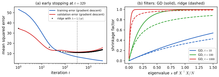
p. 455 The simplest remedy is to stop training when the validation error starts to increase (Figure 4.8 of the book). The heuristic works because it restricts how much information the optimiser can transfer from the training examples to the parameters (Achille and Soatto, 2019). In the quadratic case this has an exact meaning, derived in gap 13.13: gradient descent stopped at time \(t\) is a ridge-like shrinkage.
13.5.2 Weight decay
p. 455 A Gaussian prior \(\N(\bm w\given\bm 0,\alpha^2\bm I)\) on the weights and \(\N(\bm b\given\bm 0,\beta^2\bm I)\) on the biases, followed by MAP estimation, is \(\ell_2\) regularisation of the objective; in the neural-network literature it is called weight decay because it encourages small weights (and so simpler functions), as in ridge regression (Section 11.3).
Filling the gap 13.13: weight decay is MAP, and early stopping is a shrinkage filter close to ridge p. 455
Derivation
Weight decay = MAP. With prior \(\N(\bm w\given\bm0,\lambda^{-1}\bm I)\) the negative log posterior is \(\NLL(\bm w)+\frac\lambda2\|\bm w\|^2+\mathrm{const}\), so \(\lambda=1/\alpha^2\) when \(\NLL\) is the total (summed) negative log-likelihood. Its gradient step is \(\bm w\leftarrow\bm w-\eta(\nabla\NLL+\lambda\bm w)=(1-\eta\lambda)\bm w-\eta\nabla\NLL\): in each step the weights are first multiplied by \(1-\eta\lambda\) (they "decay") and then moved by the data gradient. Biases are usually left out of the penalty.
Early stopping in the quadratic case. Let \(L(\bm w)=\frac12(\bm w-\bm w^\ast)^\T\bm H(\bm w-\bm w^\ast)\) with \(\bm H=\bm U\diag(h_i)\bm U^\T\succeq0\); this is exactly the training loss of linear regression, \(\bm H=\bm X^\T\bm X/N\), \(\bm w^\ast\) the least-squares solution (and a local model of any smooth loss). Gradient descent from \(\bm w_0=\bm 0\) with step \(\eta\) satisfies \(\bm w_{t}-\bm w^\ast=(\bm I-\eta\bm H)^t(\bm w_0-\bm w^\ast)\), so in the eigenbasis the \(i\)-th coordinate of \(\bm w_t\) is the corresponding coordinate of \(\bm w^\ast\) multiplied by \[ g_t(h_i)=1-(1-\eta h_i)^t. \] Ridge regression with penalty \(\lambda\) (\(\bm w_\lambda=(\bm H+\lambda\bm I)^{-1}\bm H\bm w^\ast\)) multiplies it by \(r_\lambda(h)=h/(h+\lambda)\). Compare them at \(\lambda=1/(\eta t)\), writing \(x=\eta th\ge0\): \(r=x/(1+x)\), and for \(\eta h\le1\) (needed for stability) \(g_t(h)=1-(1-\eta h)^t\). Since \(1-u\le e^{-u}\), \((1-\eta h)^t\le e^{-x}\), so \(g_t\ge1-e^{-x}\ge x/(1+x)=r\) (because \(e^{-x}\le1/(1+x)\)). By Bernoulli's inequality \((1-\eta h)^t\ge1-x\), so \(g_t\le\min(1,x)\le2x/(1+x)=2r\). Hence \[ r_{1/(\eta t)}(h)\le g_t(h)\le2\,r_{1/(\eta t)}(h)\qquad\text{for all }h\in[0,1/\eta]. \] Both are soft projections that keep directions of large curvature (well determined by the data) and shrink directions of small curvature (determined mostly by noise); stopping later means a smaller effective penalty \(\lambda=1/(\eta t)\). The two filters are plotted in Figure 13.S5b. This is a statement about the quadratic model; for a deep network no such equivalence is exact, and the book's information-theoretic explanation (Achille and Soatto, 2019) is of a different kind. \(\square\)
13.5.3 Sparse DNNs
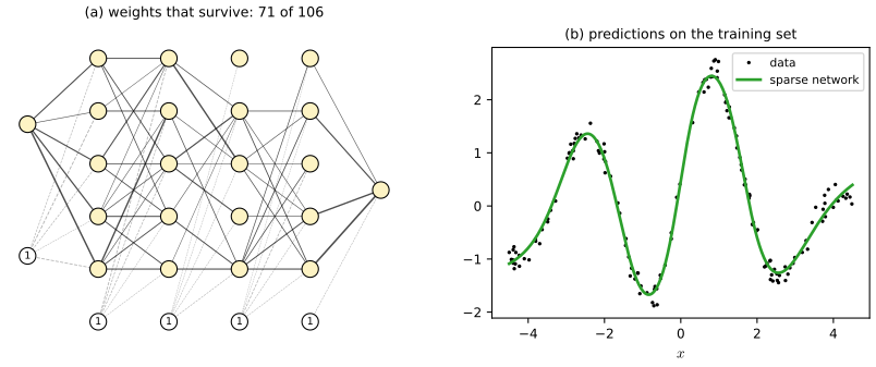
p. 455 Because networks have many weights, encouraging sparsity saves memory and time (model compression). One can use \(\ell_1\) regularisation (Section 11.4), automatic relevance determination (Section 11.7.7) or other methods. Figure 13.17 shows a 5-layer MLP fitted to 1-d regression data with an \(\ell_1\) penalty on the weights: the surviving graph is sparse. Unstructured sparsity is rarely used in practice because GPUs are optimised for dense products; group-sparsity penalties, which remove whole units or layers, give block-sparse matrices and real speedups.
Filling the gap 13.14: l1 regularisation, the proximal step and exact zeros p. 455, Figure 13.17
Derivation
Proximal operator of the \(\ell_1\) norm. For \(t>0\), \(\prox_{t|\cdot|}(z)=\argmin_x\{\tfrac12(x-z)^2+t|x|\}\). The objective is strictly convex, so the minimiser is characterised by \(0\in x-z+t\,\partial|x|\). If \(x>0\): \(x=z-t\) (requires \(z>t\)); if \(x<0\): \(x=z+t\) (requires \(z<-t\)); if \(x=0\): \(z\in[-t,t]\). So \(\prox(z)=\sign(z)\max(|z|-t,0)=:S_t(z)\), the soft threshold, applied elementwise for the full \(\ell_1\) norm.
Proximal gradient step. To minimise \(\ell(\bm w)+\lambda\|\bm w\|_1\) with \(\ell\) smooth, replace \(\ell\) by its quadratic model at \(\bm w_t\), \(\ell(\bm w_t)+\nabla\ell^\T(\bm w-\bm w_t)+\frac1{2\eta}\|\bm w-\bm w_t\|^2\); minimising model plus penalty separates over coordinates and gives \(\bm w_{t+1}=S_{\eta\lambda}(\bm w_t-\eta\nabla\ell(\bm w_t))\). Plain subgradient steps oscillate around 0 and never give exact zeros; the proximal step sets a coordinate exactly to 0 whenever \(|w_i-\eta\partial_i\ell|\le\eta\lambda\). For convex \(\ell\) with \(L\)-Lipschitz gradient and \(\eta\le1/L\) the objective converges at rate \(O(1/t)\) (Beck and Teboulle, 2009); for a neural network (non-convex) only stationarity is guaranteed. Figure 13.17 was fitted by 3000 Adam steps without penalty and then 20 000 proximal steps with \(\lambda=3\times10^{-3}\), \(\eta=0.02\).
Group sparsity. For a group \(g\) (for example all weights entering one unit) the penalty \(t\|\bm w_g\|_2\) has the proximal map \(\bm w_g\mapsto(1-t/\|\bm w_g\|)_+\bm w_g\): the whole group is set to 0 once its norm is below \(t\), which removes a unit and gives block-sparse weight matrices. \(\square\)
13.5.4 Dropout
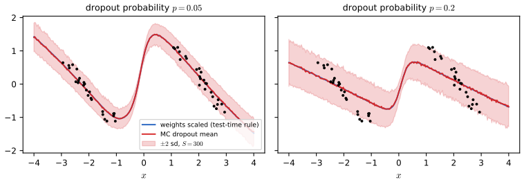
pp. 455–457 Dropout (Srivastava et al., 2014) turns off, per example, all outgoing connections of each unit with probability \(p\) (Figure 13.18, a drawing). It dramatically reduces overfitting and is widely used. The intuition is that it prevents complex co-adaptation: each unit must work even if others are missing at random. One can view it as using a noisy copy of the weights, \(\theta_{lji}=w_{lji}\epsilon_{li}\) with \(\epsilon_{li}\sim\mathrm{Ber}(1-p)\). At test time the noise is turned off and, so that the activations have the same expectation as in training, the weights are multiplied by the keep probability \(1-p\) (the "weight scaling rule"). Alternatively, keeping the noise on and averaging over \(S\) random masks gives Monte Carlo dropout, \[ p(\bm y\given\bm x,\mathcal D)\approx\frac1S\sum_{s=1}^Sp(\bm y\given\bm x,\hat{\bm W}\bm\epsilon^s+\hat{\bm b}), \tag{13.96} \] an ensemble of thinned networks that can approximate the Bayesian posterior predictive, especially if the rate is tuned (Gal and Ghahramani, 2016; Kendall and Gal, 2017).
Filling the gap 13.15: dropout as an adaptive penalty, and the weight scaling rule pp. 456–457, (13.96)
Derivation
Take one linear unit \(\hat y=\sum_iw_i\epsilon_ix_i\) with independent masks \(\epsilon_i\sim\mathrm{Ber}(q)\), \(q=1-p\).
Weight scaling. \(\E\hat y=q\sum_iw_ix_i\), so using the weights \(q\bm w\) at test time reproduces the mean output exactly (for a linear unit); the variance is \(\V\hat y=q(1-q)\sum_iw_i^2x_i^2\). Inverted dropout divides the mask by \(q\) during training, \(\hat y=\sum_iw_i\frac{\epsilon_i}{q}x_i\), so that the mean is \(\bm w^\T\bm x\) and no rescaling is needed at test time.
The induced regulariser. For inverted dropout and squared error, \[ \E\Big[\big(y-\textstyle\sum_iw_i\tfrac{\epsilon_i}q x_i\big)^2\Big]=(y-\bm w^\T\bm x)^2+\V\hat y=(y-\bm w^\T\bm x)^2+\frac{1-q}{q}\sum_iw_i^2x_i^2=(y-\bm w^\T\bm x)^2+\frac p{1-p}\sum_iw_i^2x_i^2, \] by the bias–variance split of the mean squared error (\(\E(y-\hat y)^2=(y-\E\hat y)^2+\V\hat y\)). Summed over a data set, the penalty is \(\frac p{1-p}\sum_iw_i^2\|\bm X_{:,i}\|^2\): a ridge penalty whose coefficient on weight \(i\) is proportional to the squared size of feature \(i\), i.e. an adaptive \(\ell_2\) penalty (Wager et al., 2013). With standardised features it is ordinary ridge regression with \(\lambda=Np/(1-p)\). I verified the formula by enumerating all \(2^6\) masks for a random example (both sides 0.242536).
Nonlinear networks. For a nonlinear network the weight-scaling rule is only an approximation to the average prediction over masks, not an identity (for softmax output units it is the normalised geometric mean of the ensemble; Srivastava et al., 2014); Monte Carlo dropout estimates the arithmetic average directly. For a network with identity activations the two coincide: the average of 20 000 random-mask predictions of a linear network agrees with the weight-scaled prediction to 0.03. \(\square\)
13.5.5 Bayesian neural networks
p. 457 With more parameters than data, many parameter settings fit the training set equally well and generalise differently. A Bayesian neural network (BNN) keeps the induced uncertainty by marginalising the parameters, \(p(\bm y\given\bm x,\mathcal D)=\int p(\bm y\given\bm x,\bm\theta)p(\bm\theta\given\mathcal D)\,\d\bm\theta\) (13.97): an infinite ensemble of differently weighted networks, which avoids overfitting (MacKay, 1995) and can improve accuracy (Wilson and Izmailov, 2020), but is hard to do exactly for large networks. See the sequel to the book (Murphy, 2023) and, in this site, Bishop's Section 5.7 with its Bayesian neural network demo.
13.5.6 Regularization effects of (stochastic) gradient descent *
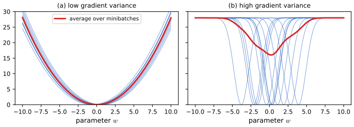
pp. 457–459 Some optimisers (second-order batch methods) find "needles in haystacks", narrow deep holes of the loss landscape (sharp minima, Figure 13.19, a sketch), which fit the training data well but tend to overfit; flat minima are more robust and generalise better, since in a flat region there is much posterior uncertainty and samples there cannot memorise irrelevant details (Achille and Soatto, 2017). SGD tends to find flat minima thanks to its noise: implicit regularisation. It can also be encouraged explicitly (entropy SGD, sharpness-aware minimisation, stochastic weight averaging). Since the loss depends on the data, we get one loss curve per minibatch (Figure 13.20): if every curve is a wide basin we are at a stable point, but if the wide overall basin is the average of many narrow ones, generalisation is likely worse.
The book quotes the analysis of Barrett and Dherin (2021) and Smith et al. (2021): gradient descent with step \(\epsilon\) follows, to second order, the gradient flow \(\dot{\bm w}=-\nabla\tilde L_{\rm GD}(\bm w)\) of the modified loss \[ \tilde L_{\rm GD}(\bm w)=L(\bm w)+\frac\epsilon4\|\nabla L(\bm w)\|^2, \tag{13.98} \] which penalises large gradients (high curvature), and for SGD with \(m\) minibatches \[ \tilde L_{\rm SGD}(\bm w)=L(\bm w)+\frac\epsilon{4m}\sum_{k=1}^m\|\nabla L_k(\bm w)\|^2=\tilde L_{\rm GD}(\bm w)+\frac\epsilon{4m}\sum_{k=1}^m\|\nabla L_k(\bm w)-\nabla L(\bm w)\|^2, \tag{13.99, 13.100} \] where the last term is the variance of the minibatch gradients, a measure of stability. So SGD has statistical as well as computational advantages over full-batch gradient descent.
Filling the gap 13.16: the modified loss of gradient descent and of shuffled SGD pp. 458–459, (13.98)–(13.100)
Derivation
Gradient descent (13.98). The GD step is \(\bm w_{t+1}=\bm w_t+\epsilon\bm f_0(\bm w_t)\) with \(\bm f_0=-\nabla L\). Look for a vector field \(\tilde{\bm f}=\bm f_0+\epsilon\bm f_1\) whose flow for time \(\epsilon\) agrees with the step up to \(O(\epsilon^3)\). Taylor expansion of the flow \(\dot{\bm w}=\tilde{\bm f}(\bm w)\) over time \(\epsilon\): \[ \bm w(\epsilon)=\bm w+\epsilon\tilde{\bm f}+\frac{\epsilon^2}2D\tilde{\bm f}\,\tilde{\bm f}+O(\epsilon^3)=\bm w+\epsilon\bm f_0+\epsilon^2\big(\bm f_1+\tfrac12D\bm f_0\,\bm f_0\big)+O(\epsilon^3). \] Matching \(\bm w+\epsilon\bm f_0\) requires \(\bm f_1=-\frac12D\bm f_0\,\bm f_0\). Here \(D\bm f_0=-\bm H\) (the Hessian of \(L\)), so \(\bm f_1=-\frac12\bm H\nabla L=-\frac14\nabla\|\nabla L\|^2\), because \(\nabla\|\nabla L\|^2=2\bm H\nabla L\). Therefore \(\tilde{\bm f}=-\nabla\big(L+\frac\epsilon4\|\nabla L\|^2\big)\), which is (13.98). The local error per step is \(O(\epsilon^3)\), so after a time \(T=\epsilon t\) the flow of \(\tilde L\) is within \(O(\epsilon^2)\) of the GD iterates, while the flow of \(L\) alone is within \(O(\epsilon)\) only. Figure 13.S3a confirms the two rates on logistic regression for the iris data: the log-log slopes of the distance at time \(T=2\) are 1.02 (flow of \(L\)) and 2.01 (flow of \(\tilde L\)).
Shuffled SGD (13.99). Let \(L=\frac1m\sum_kL_k\), \(\bm g_k=\nabla L_k\), \(\bm H_k=\nabla^2L_k\). One epoch visits the \(m\) minibatches in a random order \(\pi\): \(\bm w^{(k)}=\bm w^{(k-1)}-\epsilon\bm g_{\pi(k)}(\bm w^{(k-1)})\). Expanding \[ \bm g_{\pi(k)}(\bm w^{(k-1)})=\bm g_{\pi(k)}(\bm w)-\epsilon\bm H_{\pi(k)}\sum_{j<k}\bm g_{\pi(j)}+O(\epsilon^2) \] (all at the starting point \(\bm w\)) gives \[ \bm w^{(m)}-\bm w=-\epsilon\sum_k\bm g_k+\epsilon^2\sum_{k}\sum_{j<k}\bm H_{\pi(k)}\bm g_{\pi(j)}+O(\epsilon^3). \] Average over a uniformly random permutation: every ordered pair of distinct batches \((a,b)\) has \(a\) after \(b\) with probability \(\frac12\), so \[ \E_\pi\sum_k\sum_{j<k}\bm H_{\pi(k)}\bm g_{\pi(j)}=\frac12\sum_{a\ne b}\bm H_a\bm g_b=\frac12\big(m^2\bm H\nabla L-\sum_a\bm H_a\bm g_a\big) \] with \(\bm H=\frac1m\sum\bm H_a\). Thus \[ \E_\pi[\bm w^{(m)}-\bm w]=-\epsilon m\nabla L+\frac{\epsilon^2m^2}2\bm H\nabla L-\frac{\epsilon^2}2\sum_a\bm H_a\bm g_a+O(\epsilon^3). \] Now compare with the flow of \(\tilde L_{\rm SGD}\) over time \(T=m\epsilon\). Its field is \(-\nabla L-\frac\epsilon{2m}\sum_a\bm H_a\bm g_a\) (since \(\nabla\|\bm g_a\|^2=2\bm H_a\bm g_a\)), and the flow's second-order expansion gives \(-m\epsilon\nabla L-\frac{\epsilon^2}2\sum_a\bm H_a\bm g_a+\frac{m^2\epsilon^2}2\bm H\nabla L+O(\epsilon^3)\): the same. So, on average over shuffles, one epoch of SGD matches the flow of (13.99) for time \(m\epsilon\) to \(O(\epsilon^3)\), whereas matching the flow of \(L\) is only \(O(\epsilon^2)\). The numerical experiment averages all \(5!=120\) shuffles of five minibatches for logistic regression: the errors scale with \(\epsilon\) like \(\epsilon^{2.8}\) (modified loss) against \(\epsilon^{1.8}\) (plain flow). (The exponents are slightly below 3 and 2 because the expansion has \(O(\epsilon^4)\) terms of non-negligible size at the step sizes used.)
The variance identity (13.100). Since \(\frac1m\sum_k\bm g_k=\nabla L\), \(\frac1m\sum_k\|\bm g_k\|^2=\|\nabla L\|^2+\frac1m\sum_k\|\bm g_k-\nabla L\|^2\) (the usual \(\E\|X\|^2=\|\E X\|^2+\mathrm{tr}\,\mathrm{cov}\,X\)), which gives (13.100) at once. The regulariser is smaller for larger batches (less variance), so small batches regularise more. \(\square\)
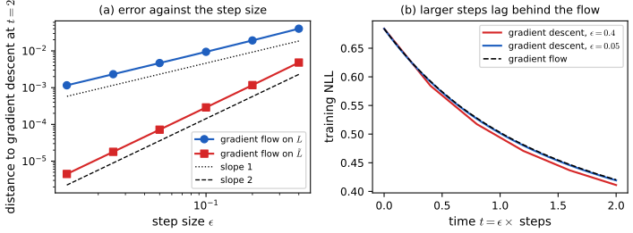
13.5.7 Over-parameterized models
p. 459 Modern networks have far more parameters \(P\) than training examples \(N\) and typically reach zero training loss. Yet they often generalise better than models with \(P\ll N\). For \(P<N\) the usual U-shaped test-error curve appears, with the bias-variance trade-off of Section 4.7.6.3; for \(P>N\) the test error falls again: double descent (Belkin et al., 2019; Nakkiran et al., 2019). Intuitively, at \(P=N\) the model needs a very non-smooth function to interpolate, while for \(P\gg N\) it can interpolate with a smooth one (Bubeck and Sellke, 2021).
Filling the gap 13.17: double descent for minimum-norm interpolation, in closed form p. 459
Derivation
Setting. Data \(y=\bm X\bm\theta^\ast+\bm\varepsilon\) with \(\bm X\in\R^{N\times P}\) having iid \(\N(0,1)\) entries and \(\bm\varepsilon\sim\N(\bm0,\sigma^2\bm I)\), test inputs from the same law. The estimator is the least-norm least-squares solution \(\hat{\bm\theta}=\bm X^+\bm y\) (the pseudo-inverse): ordinary least squares for \(P\le N\), and for \(P\ge N\) the interpolator \(\bm X^\T(\bm X\bm X^\T)^{-1}\bm y\). For \(P>N\) it is the minimum-norm interpolator: any interpolant is \(\hat{\bm\theta}+\bm v\) with \(\bm X\bm v=\bm0\), and \(\bm v\) is orthogonal to the row space that contains \(\hat{\bm\theta}\), so \(\|\hat{\bm\theta}+\bm v\|^2=\|\hat{\bm\theta}\|^2+\|\bm v\|^2\).
Risk for \(P\ge N+2\). Let \(\bm\Pi=\bm X^+\bm X\) be the orthogonal projection onto the row space (rank \(N\)). Then \(\hat{\bm\theta}-\bm\theta^\ast=-(\bm I-\bm\Pi)\bm\theta^\ast+\bm X^+\bm\varepsilon\), and the excess test risk (isotropic features) is \(\|\hat{\bm\theta}-\bm\theta^\ast\|^2\). The two terms are uncorrelated (\(\bm\varepsilon\) is independent of \(\bm X\) and mean zero). Bias: the row space of a Gaussian matrix is a uniformly random \(N\)-dimensional subspace, so \(\E\bm\Pi=\frac NP\bm I\) by rotation invariance (trace \(N\)), giving \(\E\|(\bm I-\bm\Pi)\bm\theta^\ast\|^2=(1-\frac NP)\|\bm\theta^\ast\|^2\). Variance: \(\|\bm X^+\bm\varepsilon\|^2=\bm\varepsilon^\T(\bm X\bm X^\T)^{-1}\bm\varepsilon\), with expectation \(\sigma^2\,\E\,\mathrm{tr}(\bm X\bm X^\T)^{-1}\). By symmetry the \(N\) diagonal entries of \((\bm X\bm X^\T)^{-1}\) have the same mean, and by the Schur complement formula \([(\bm X\bm X^\T)^{-1}]_{11}=1/(\bm x_1^\T(\bm I-\bm\Pi_{-1})\bm x_1)\), where \(\bm x_1\) is the first row of \(\bm X\) and \(\bm\Pi_{-1}\) the projection onto the span of the other \(N-1\) rows (rank \(N-1\)). Given them, \(\bm x_1^\T(\bm I-\bm\Pi_{-1})\bm x_1\sim\chi^2_{P-N+1}\), and \(\E[1/\chi^2_k]=1/(k-2)\) for \(k>2\). Hence \(\E\,\mathrm{tr}(\bm X\bm X^\T)^{-1}=\frac N{P-N-1}\) (the mean of an inverse Wishart matrix), and \[ \text{excess risk}=\Big(1-\frac NP\Big)\|\bm\theta^\ast\|^2+\sigma^2\frac N{P-N-1}\qquad(P\ge N+2). \]
Risk for \(P\le N-2\). Ordinary least squares is unbiased; the same argument with \((\bm X^\T\bm X)^{-1}\sim\) inverse Wishart gives variance \(\sigma^2\frac P{N-P-1}\).
Reading the formulas. Both variance terms blow up as \(P\to N\) from either side (there \(\bm X\) has a tiny singular value and the solution must stretch enormously to fit the noise): the peak of double descent. For \(P\to\infty\) the variance term decays like \(\sigma^2N/P\) and the bias tends to \(\|\bm\theta^\ast\|^2\): the interpolant spreads its fit over so many directions that each one carries little noise, but if the signal itself lives in a fixed number of features the extra dimensions are noise-like directions that absorb the label noise harmlessly. To make both sides comparable in Figure 13.S4, the true model has \(D=400\) features with equally sized coefficients, \(\|\bm\theta^\ast\|^2=1\), and the fit uses only the first \(P\); the omitted features act as extra noise of variance \((1-P/D)\|\bm\theta^\ast\|^2\) (independent of the fitted columns for Gaussian features), so replace \(\sigma^2\) by \(\sigma^2+(1-P/D)\) and \(\|\bm\theta^\ast\|^2\) by \(P/D\) in the formulas. The simulation (300 data sets per point, \(N=40\), \(\sigma^2=0.05\)) agrees with the closed form within 6 percent at \(P=10,30,70,150,400\), and the inverse-Wishart mean was confirmed separately. At exactly \(P=N\) the expectation is infinite. \(\square\)
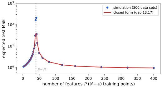
See also: Foundations of Deep Learning, Section 9.3.2 (double descent); Introduction to Statistical Learning, Section 10.8 (interpolation and double descent).
13.6 Other kinds of feedforward networks *
13.6.1 Radial basis function networks
pp. 459–461 A one-layer network whose hidden layer is the feature vector \[ \bm\phi(\bm x)=[K(\bm x,\bm\mu_1),\dots,K(\bm x,\bm\mu_K)], \tag{13.101} \] with centroids (exemplars) \(\bm\mu_k\in\mathcal X\) and a kernel \(K(\bm x,\bm\mu)\ge0\), is an RBF network (Broomhead and Lowe, 1988). The usual choice is the Gaussian kernel \[ K_{\rm gauss}(\bm x,\bm c)=\exp\Big(-\frac1{2\sigma^2}\|\bm c-\bm x\|_2^2\Big), \tag{13.102, 13.103} \] with bandwidth \(\sigma\), shift invariant (a function of \(r=\|\bm x-\bm c\|\) only). The model is \(p(\bm y\given\bm x;\bm\theta)=p(\bm y\given\bm w^\T\bm\phi(\bm x))\) (13.104) with \(\bm\theta=(\bm\mu,\bm w)\). With fixed centroids the weights solve a (regularised) least-squares or logistic problem (Chapter 11); unknown centroids can be estimated by clustering (K-means, Section 21.3); or one centroid per data point, \(\bm\mu_n=\bm x_n\), gives a non-parametric model (\(K=N\)) that can interpolate and may overfit, remedied by sparse weights (a sparse kernel machine, Sections 17.3, 17.4.1) or by integrating out \(\bm w\) (a Gaussian process, Section 17.2).
See also: Bayesian and Probabilistic ML, Section 6.3 (radial basis function networks), its kernel functions demo and Gaussian process regression demo; Elements of Statistical Learning, Chapter 6.
13.6.1.1 RBF network for regression
p. 460 Define \(p(y\given\bm x,\bm\theta)=\N(\bm w^\T\bm\phi(\bm x),\sigma^2)\). With \(K=10\) equally spaced prototypes the bandwidth controls the fit (Figure 13.22): small \(\sigma\) makes each bump local, so the fit is spiky between prototypes, and the design matrix is nearly diagonal; a large \(\sigma\) makes the features overlap, and for \(\sigma\to\infty\) the columns of the design matrix become the constant 1, collapsing the model towards a low-order polynomial (see gap 13.18 for what exactly happens).
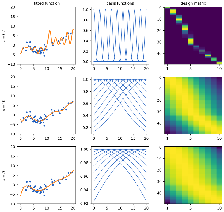
numpy.linalg.lstsq, which drops singular values below \(10^{-14}\) of the largest, so the \(\sigma=50\) fit is a smooth low-order curve and not a straight line (gap 13.18). Simulated data. Reproduces Murphy (2022), Figure 13.22. PDF · SVG13.6.1.2 RBF network for classification
pp. 460–461 For binary classification use \(p(y\given\bm x;\bm\theta)=\operatorname{Ber}(\sigma(\bm w^\T\bm\phi(\bm x)))\). For the XOR function (Figure 13.21a), the book states that a degree-10 polynomial logistic regression cannot separate the (jittered) data, but an RBF network with the four prototypes (the four corners, crosses in (c)) solves it. The second half is right; the first is not, see the gap box.
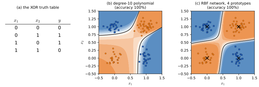
Filling the gap 13.18: RBF networks, the flat limit and XOR pp. 459–461, (13.101)–(13.104)
Derivation
Fitting. With centroids fixed, \(\bm\Phi\in\R^{N\times(K+1)}\) (a column of ones for the intercept and \(\phi_k(\bm x_n)=K(\bm x_n,\bm\mu_k)\)), the model is linear in \(\bm w\): regression gives the ridge normal equations \((\bm\Phi^\T\bm\Phi+\lambda\bm I')\bm w=\bm\Phi^\T\bm y\) (Chapter 11), classification a convex logistic problem solved by Newton's method (Chapter 10). With one centroid at each training point (\(K=N\)) and distinct points, the Gaussian kernel matrix \(\bm\Phi_{nk}=e^{-\|\bm x_n-\bm x_k\|^2/2\sigma^2}\) is symmetric positive definite (Gaussian kernels are positive definite for distinct points), so \(\lambda\to0\) gives exact interpolation of any targets; hence the overfitting the book warns about.
The flat limit \(\sigma\to\infty\). The book says that for a huge bandwidth the design matrix is a constant matrix of ones "hence the corresponding function is just a straight line". The features do become nearly constant (the third column of Figure 13.22 shows entries between 0.92 and 1), but what unpenalised least squares does depends on how the nearly dependent columns are treated. Expand \(\phi_k(x)=1-\frac{(x-\mu_k)^2}{2\sigma^2}+\frac{(x-\mu_k)^4}{8\sigma^4}-\cdots\): the differences between features carry polynomials of increasing degree, at increasing orders of \(\sigma^{-2}\), and in exact arithmetic the least-squares fit can use them, with large weights of opposite signs. It is known that as \(\sigma\to\infty\) Gaussian RBF interpolants and least-squares fits converge to polynomial ones (Driscoll and Fornberg, 2002; Schaback, 2005). I confirmed it in 300-digit arithmetic for \(K=10\) centres plus the intercept (11 parameters): the exact least-squares RBF fit at \(\sigma=50\) is within 0.004 (maximum over the 50 data points) of the degree-10 polynomial least-squares fit, at \(\sigma=2000\) within \(2.5\times10^{-6}\), whereas it is 2.7 away from the straight-line fit. So the flat limit of an unpenalised fit is a polynomial of degree \(K\) and not a line. A straight line appears when the weights are penalised heavily (ridge with a penalty large compared with the tiny singular values) or when a numerical routine discards the small singular values so that only the constant and the leading variation survive; the book's third row is of that kind. In Figure 13.22 the double-precision lstsq keeps the seven largest of the eleven singular values (those above \(1.1\times10^{-14}\) of the largest), which is why my \(\sigma=50\) fit is a smooth low-order curve (the demonstration, which uses ridge \(\lambda=10^{-4}\), has about 3.0 effective parameters at \(\sigma=50\)).
XOR with four prototypes: an explicit separator. Let \(\bm c_{ab}=(a,b)\) be the corners and \(\phi_{ab}(\bm x)=e^{-\|\bm x-\bm c_{ab}\|^2/2\sigma^2}\). At a corner \(\bm c_{ab}\) the four features are \(1\), \(e^{-1/2\sigma^2}\) (twice, the neighbours at distance 1) and \(e^{-1/\sigma^2}\) (the opposite corner, distance \(\sqrt2\)). Take \(\bm w=(-a_0,+a_0,+a_0,-a_0)\) on \((\phi_{00},\phi_{01},\phi_{10},\phi_{11})\) and bias 0 with \(a_0>0\). At \(\bm c_{01}\): \(\bm w^\T\bm\phi=a_0(1+e^{-1/\sigma^2})-2a_0e^{-1/2\sigma^2}=a_0(1-e^{-1/2\sigma^2})^2>0\); at \(\bm c_{00}\): \(-a_0(1-e^{-1/2\sigma^2})^2<0\); the other two are symmetric. So the labels of the four corners are separated with margin \(a_0(1-e^{-1/2\sigma^2})^2\), and by continuity the jittered points near the corners are too, which is what Figure 13.21c shows. Two prototypes nearly suffice: with the centres \((0,0)\) and \((1,1)\) (the class-0 corners) the feature sum \(\phi_{00}+\phi_{11}\) is large exactly on the class-0 corners (98 percent training accuracy on the jittered points).
The book's claim about polynomials is incorrect. XOR on \(\{0,1\}^2\) is \(y=\ind\big((x_1-\tfrac12)(x_2-\tfrac12)<0\big)\), and \((x_1-\frac12)(x_2-\frac12)\) is a polynomial of degree 2. A logistic regression on the monomials up to degree 2 with logit \(-k(x_1-\frac12)(x_2-\frac12)\) therefore separates the four corners (and the jittered clouds as long as the jitter is below \(\frac12\)). A degree-10 expansion contains all of these monomials. In the code, Newton's method on \((1,x_1,x_2,x_1x_2)\) gives 0 training errors on the 100 jittered points, and so does scikit-learn's default penalised fit on the degree-10 expansion (Figure 13.21b). The failure shown in the book must come from the optimiser, the scaling of the monomials or the penalty, not from the model class. \(\square\)
13.6.2 Mixtures of experts
pp. 461–463 A unimodal output distribution (Gaussian or Student) whose mean and variance depend on \(\bm x\), \(p(\bm y\given\bm x)=\N(\bm y\given f_\mu(\bm x),\diag(\sigma_+(f_\sigma(\bm x))))\) (13.105), fails on one-to-many functions, where an input has several equally likely outputs: 3-d pose from a single image, colourisation of a grey-scale image, prediction of video frames. A model trained by maximum likelihood with a unimodal density produces a blurry average. The fix is a conditional mixture model, \[ p(\bm y\given\bm x)=\sum_{k=1}^Kp(\bm y\given\bm x,z=k)\,p(z=k\given\bm x), \tag{13.106} \] \[ p(\bm y\given\bm x,z=k)=\N(\bm y\given f_{\mu,k}(\bm x),\diag(f_{\sigma,k}(\bm x))),\qquad p(z=k\given\bm x)=\mathrm{Cat}(z\given\softmax(f_z(\bm x))), \tag{13.107, 13.108} \] a mixture of experts (MoE; Jacobs et al., 1991; Jordan and Jacobs, 1994). The \(k\)-th submodel is an "expert" in a region of input space; \(p(z=k\given\bm x)\) is the gating function, which decides which expert to use, and picking the most likely expert activates only a subset of the model (conditional computation; Shazeer et al., 2017). It is trained by SGD or by EM (Section 8.7.3).
See also: Bayesian and Probabilistic ML, Section 14.5 (conditional mixture models), its mixture of experts demo and mixture density demo; Foundations of Deep Learning, Section 6.5 (mixture density networks).
13.6.2.1 Mixture of linear experts
p. 463 With linear experts and a linear gate, \(p(y\given\bm x,z=k,\bm\theta)=\N(y\given\bm w_k^\T\bm x,\sigma_k^2)\) and \(p(z=k\given\bm x,\bm\theta)=\mathrm{Cat}(z\given\softmax_k(\bm V\bm x))\) (13.109, 13.110); the gating value is the responsibility of expert \(k\) for input \(\bm x\). Figure 13.23 fits three linear experts to a one-to-many data set: the gate softly partitions the input, each expert is a line, the weighted mean of the experts (red) is a poor prediction in the ambiguous region, while the prediction of the single most responsible expert (black) is far better.
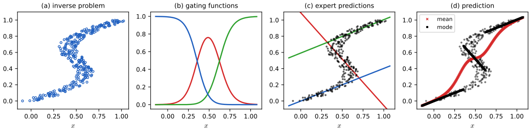
13.6.2.2 Mixture density networks
p. 463 If the gating function and the experts are DNNs the model is a mixture density network (MDN; Bishop, 1994) or deep mixture of experts (Eigen et al., 2013; Figure 13.24, a drawing).
13.6.2.3 Hierarchical MoEs
p. 463 If each expert is itself an MoE the model is a hierarchical mixture of experts (Jordan and Jacobs, 1994; Figure 13.25, a drawing): with \(L\) levels it is a "soft" decision tree of depth \(L\) in which each example goes through every branch and the prediction is a weighted average (decision trees: Section 18.1).
Filling the gap 13.19: regression to the mean, the moments of a mixture, and EM for mixtures of experts pp. 461–463, (13.105)–(13.110)
Derivation
Why a unimodal model regresses to the mean. For a Gaussian with fixed variance the population NLL is \(\E\big[\frac{(y-f(\bm x))^2}{2\sigma^2}\big]+\mathrm{const}\), minimised over functions \(f\) by \(f(\bm x)=\E[y\given\bm x]\): for each \(\bm x\), \(\E[(y-f)^2\given\bm x]=\V[y\given\bm x]+(\E[y\given\bm x]-f)^2\). If the conditional law is bimodal, say \(\frac12\N(-2,0.1^2)+\frac12\N(2,0.1^2)\), the optimal mean is 0, where the density is essentially zero, and the optimal variance is \(\approx4\): the model predicts a value that never occurs. Letting the variance depend on \(\bm x\) does not help: it only widens the band around the same mean.
Mean and variance of a mixture. With gate probabilities \(\pi_k(\bm x)\), expert means \(\mu_k(\bm x)\) and variances \(\sigma_k^2(\bm x)\): \(\E[y\given\bm x]=\sum_k\pi_k\mu_k\) and, by the law of total variance, \(\V[y\given\bm x]=\sum_k\pi_k\sigma_k^2+\sum_k\pi_k\mu_k^2-(\sum_k\pi_k\mu_k)^2\) (within-expert plus between-expert variance). The "mean" curve of Figure 13.23d is the first of these; it can lie where the density is zero. The "mode" curve selects \(k^\ast(\bm x)=\argmax_k\pi_k(\bm x)\) and predicts \(\mu_{k^\ast}(\bm x)\), a good approximation to a mode of the mixture when the experts are well separated. (The exact mode of a Gaussian mixture is not available in closed form.)
EM for the mixture of linear experts. The complete-data log-likelihood with latent \(z_n\) is \(\sum_n\sum_k\ind(z_n=k)[\log\pi_k(\bm x_n)+\log\N(y_n\given\bm w_k^\T\bm x_n,\sigma_k^2)]\). E-step: replace the indicator by the responsibility \(r_{nk}=\pi_k(\bm x_n)\N(y_n\given\bm w_k^\T\bm x_n,\sigma_k^2)\big/\sum_j\pi_j(\bm x_n)\N(y_n\given\bm w_j^\T\bm x_n,\sigma_j^2)\). M-step: the objective separates into (i) for each expert a weighted least-squares problem, \(\bm w_k=(\bm X^\T\bm R_k\bm X)^{-1}\bm X^\T\bm R_k\bm y\) with \(\bm R_k=\diag(r_{nk})\) and \(\sigma_k^2=\sum_nr_{nk}(y_n-\bm w_k^\T\bm x_n)^2/\sum_nr_{nk}\) (the weighted Gaussian MLE); and (ii) for the gate a softmax regression with the soft labels \(r_{nk}\), \(\max_{\bm V}\sum_n\sum_kr_{nk}\log\softmax_k(\bm V\bm x_n)\), a concave problem with gradient \(\sum_n(\bm r_n-\bm\pi_n)\bm x_n^\T\), solved by a few Newton or Bohning-bound steps (Section 10.3.4). EM never decreases the log-likelihood (Section 8.7.3): in the run of Figure 13.23 it rises from 46.7 (after 5 iterations) through 304.9 (60) to 318.3 (200). Because the experts are exchangeable, the solution is only defined up to a relabelling of components, and different initialisations reach different local maxima, so the code keeps the best of eight restarts.
Hierarchies. For a two-level model \(p(y\given\bm x)=\sum_k\pi_k(\bm x)\sum_j\pi_{j\mid k}(\bm x)\N(y\given\mu_{kj}(\bm x),\sigma_{kj}^2)\): a flat mixture whose weights are products of gates along a path of a soft tree. \(\square\)
13.7 Exercises
The one exercise of Chapter 13 (Murphy, 2022, pp. 463–465), restated in my own words, with a complete solution (hidden). The book names the second weight matrix both \(\bm U\) and \(\bm V\); here it is \(\bm U\) throughout.
Exercise 13.1 (backpropagation for an MLP). Consider a classification MLP with one hidden layer, input \(\bm x\in\R^D\), \(\bm z=\bm W\bm x+\bm b_1\in\R^K\), \(\bm h=\ReLU(\bm z)\in\R^K\), \(\bm a=\bm U\bm h+\bm b_2\in\R^C\) and loss \(L=\mathrm{CE}(\bm y,\softmax(\bm a))\in\R\) for a one-hot \(\bm y\), where \(\bm W\in\R^{K\times D}\), \(\bm U\in\R^{C\times K}\). Show that \[ \nabla_{\bm U}L=\bm\delta_1\bm h^\T,\quad\nabla_{\bm b_2}L=\bm\delta_1,\quad\nabla_{\bm W}L=\bm\delta_2\bm x^\T,\quad\nabla_{\bm b_1}L=\bm\delta_2,\quad\nabla_{\bm x}L=\bm W^\T\bm\delta_2, \tag{13.116–13.120} \] with the error signals \(\bm\delta_1=\nabla_{\bm a}L=\bm p-\bm y\) and \(\bm\delta_2=\nabla_{\bm z}L=(\bm U^\T\bm\delta_1)\odot\Heav(\bm z)\), \(\Heav\) the Heaviside function (13.121, 13.122); here the gradient has the shape of the variable it is taken with respect to.
Solution
Output layer. By (13.39) (derived in gap 13.6), \(\bm\delta_1=\nabla_{\bm a}L=\bm p-\bm y\), because \(L=\log\sum_je^{a_j}-\bm y^\T\bm a\) for \(\sum_cy_c=1\).
Second linear layer. \(a_c=\sum_kU_{ck}h_k+b_{2,c}\). Then \(\partial L/\partial U_{ck}=\delta_{1,c}h_k\) and \(\partial L/\partial b_{2,c}=\delta_{1,c}\), i.e. \(\nabla_{\bm U}L=\bm\delta_1\bm h^\T\in\R^{C\times K}\) and \(\nabla_{\bm b_2}L=\bm\delta_1\in\R^C\). Also \(\partial L/\partial h_k=\sum_c\delta_{1,c}U_{ck}\), i.e. \(\nabla_{\bm h}L=\bm U^\T\bm\delta_1\in\R^K\).
ReLU. \(h_k=\ReLU(z_k)\) depends on \(z_k\) only, with derivative \(\ind(z_k>0)=\Heav(z_k)\) (any value in \([0,1]\) at \(z_k=0\); take 0). So \(\delta_{2,k}=\partial L/\partial z_k=(\partial L/\partial h_k)\Heav(z_k)\), i.e. \(\bm\delta_2=(\bm U^\T\bm\delta_1)\odot\Heav(\bm z)\in\R^K\).
First linear layer. \(z_k=\sum_jW_{kj}x_j+b_{1,k}\) gives \(\partial L/\partial W_{kj}=\delta_{2,k}x_j\), \(\partial L/\partial b_{1,k}=\delta_{2,k}\) and \(\partial L/\partial x_j=\sum_k\delta_{2,k}W_{kj}\): \(\nabla_{\bm W}L=\bm\delta_2\bm x^\T\in\R^{K\times D}\), \(\nabla_{\bm b_1}L=\bm\delta_2\), \(\nabla_{\bm x}L=\bm W^\T\bm\delta_2\in\R^D\). \(\square\)
Numerical confirmation. For \(D=5\), \(K=4\), \(C=3\), random parameters and a random input, the five gradients computed by these formulas agree with central finite differences (step \(10^{-6}\)) to within \(2\times10^{-10}\) in the largest entry (
exercise_13_1in the code), and the general recursion agrees with PyTorch autograd.
Demonstrations
| Page | What it shows | In the notes |
|---|---|---|
| An MLP on two-dimensional data | Train a small MLP by full-batch Adam or gradient descent on circles, XOR, moons or spirals: decision map, loss curve, and a map of every hidden unit; choose depth, width, activation, weight decay and random start. Presets: 1 circles with two hidden layers; 2 linear activations collapse; 3 XOR with two units, a plateau; 4 two spirals, three hidden layers; 5 weight decay on the moons. | 13.2.1, 13.2.4, 13.5.2, gap 13.1 |
| Vanishing and exploding gradients | The size of the activations, of the backpropagated gradient and of the weight gradients across up to 60 layers, for sigmoid, tanh, ReLU and SELU, any weight scale, with or without residual blocks. Presets: 1 sigmoid vanishes; 2 ReLU with c = 1; 3 He initialisation; 4 ReLU with c = 2 explodes; 5 residual blocks; 6 SELU. | 13.4.2, 13.4.4, 13.4.5, gap 13.8, gap 13.10, gap 13.11 |
| Forward and reverse mode on a computation graph | The graph of (13.56) with values, adjoints (reverse mode) and tangents (forward mode) at chosen \((x_1,x_2)\), and the multiply-add count of a whole Jacobian for a chain with \(n\) inputs and \(m\) outputs. Presets: 1 reverse mode; 2 forward, seed \(x_1\); 3 forward, seed \(x_2\); 4 64 inputs, scalar output; 5 2 inputs, 64 outputs. | 13.3.1, 13.3.4, gap 13.5, gap 13.7 |
| Radial basis function networks | RBF regression with a chosen bandwidth, number of centres and ridge penalty, showing the fit, the basis functions and the design matrix; XOR classification with four, two or no prototypes. Presets: 1 sigma = 0.5; 2 sigma = 10; 3 sigma = 50; 4 XOR with four prototypes; 5 XOR without prototypes. | 13.6.1, gap 13.18 |
The Python code that produces every figure of this page is code/ch13_neural_networks_tabular.py (see the code index). Companion demos: backpropagation, forward and reverse mode, initialization and depth, early stopping, dropout, mixture of experts.
Notes on the book
Points where the book is imprecise or wrong
- Section 13.3.1, the cost of forward mode. The book states that for \(m=1\) and \(n=m_1=m_2=m_3\) the cost of computing \(\bm J_f(\bm x)\) is \(O(n^2)\) for both forward and reverse mode. One forward-mode pass costs \(O(n^2)\), but \(n\) passes are needed, so forward mode costs \(O(n^3)\); only reverse mode costs \(O(n^2)\) (gap 13.5, Figure 13.S7).
- (13.73), (13.74), (13.77), (13.78): Jacobians against vector-Jacobian products. \(\partial\bm z/\partial\bm x\) for a ReLU layer is \(\diag(\ind(\bm z>0))\bm W\) (an \(m\times n\) matrix); the printed \(\bm W^\T\ind(\bm z>0)\) has the wrong shape and is the VJP form \(\bm W^\T(\bm u\odot\ind(\bm z>0))\) with \(\bm u=\bm 1\). Similarly \(\diag(\bm z(1-\bm z)^\T)\bm W\) in (13.73) should read \(\diag(\bm z\odot(1-\bm z))\bm W\), and the weight "Jacobians" (13.74), (13.78) are VJPs for the upstream vector \(\bm u=\bm 1\) (gap 13.6).
- Exercise 13.1. The model is written with the second weight matrix \(\bm U\), but (13.116) and (13.122) use \(\bm V\); \(\nabla_{\bm V}L\) should be \(\nabla_{\bm U}L\) and \(\bm V^\T\) in \(\bm\delta_2\) should be \(\bm U^\T\).
- (13.39), the cross-entropy gradient. The gradient is \(\bm p-\bm y\) only when the entries of \(\bm y\) sum to 1; for unnormalised label weights it is \((\sum_cy_c)\bm p-\bm y\) (gap 13.6).
- (13.69) and the sentence after it. \(\partial L/\partial\bm z_l=\bm J_l\bm g_{l+1}\) uses the row-vector convention for the gradient while the book's gradients are column vectors; as columns it is \(\bm J_l^\T\bm g_{l+1}\), and the contribution of the top layer is \((\bm J^\T)^{L-l}\bm g_L\) rather than \(\bm J^{L-l}\bm g_L\). The spectral radius is the same, so the conclusion is unaffected (gap 13.8).
- (13.91), the residual-network gradient. It is correct only if \(\partial F_i(\bm z_i)/\partial\bm z_l\) is read as the total derivative through all intermediate layers; in terms of local Jacobians the matrix is \(\prod_i(\bm I+\bm J_i)=\bm I+\sum_i\bm J_i+\sum_{i>j}\bm J_i\bm J_j+\cdots\) (gap 13.10).
- Section 13.6.1.2 and Figure 13.21b. A degree-10 (indeed degree-2) polynomial feature expansion does separate the XOR data, since \(y=\ind((x_1-\frac12)(x_2-\frac12)<0)\) is a quadratic; in my runs a standard penalised logistic regression on the degree-10 expansion has 100 percent training accuracy. The statement that it cannot is wrong, whatever produced the book's picture (gap 13.18).
- Section 13.6.1.1, bandwidth 50. For \(\sigma\to\infty\) the features become nearly constant, but unpenalised least squares in exact arithmetic then tends to a polynomial of degree \(K\), not to a straight line; a line needs a strong penalty or truncation of small singular values (gap 13.18).
- (13.98)–(13.99), the modified loss of SGD. The result of Smith et al. (2021) describes the expected path over random shuffles of an epoch, as a flow for time \(m\epsilon\); the book presents it as a flow with a single learning rate \(\epsilon\) per step without saying that it is an average over orderings (gap 13.16).
- Step function at 0. (13.4) defines \(\Heav(a)=\ind(a\ge0)\) and Sections 13.2.7 and 13.3.3.2 use \(\ind(a>0)\); the two differ only at \(a=0\) and the XOR network never evaluates there (gap 13.1).
References
- Murphy, K. P. (2022). Probabilistic Machine Learning: An Introduction. MIT Press, Cambridge, MA. Chapter 13, pp. 425–465. probml.github.io/pml-book/book1.html.
- Achille, A. and Soatto, S. (2019). Where is the information in a deep neural network? arXiv:1905.12213.
- Barrett, D. G. T. and Dherin, B. (2021). Implicit gradient regularization. International Conference on Learning Representations.
- Baur, W. and Strassen, V. (1983). The complexity of partial derivatives. Theoretical Computer Science, 22(3), 317–330.
- Beck, A. and Teboulle, M. (2009). A fast iterative shrinkage-thresholding algorithm for linear inverse problems. SIAM Journal on Imaging Sciences, 2(1), 183–202.
- Belkin, M., Hsu, D., Ma, S. and Mandal, S. (2019). Reconciling modern machine-learning practice and the classical bias-variance trade-off. Proceedings of the National Academy of Sciences, 116(32), 15849–15854.
- Bishop, C. M. (1994). Mixture density networks. Technical report NCRG/94/004, Aston University.
- Bishop, C. M. (2006). Pattern Recognition and Machine Learning. Springer, New York.
- Broomhead, D. S. and Lowe, D. (1988). Multivariable functional interpolation and adaptive networks. Complex Systems, 2, 321–355.
- Bubeck, S. and Sellke, M. (2021). A universal law of robustness via isoperimetry. Advances in Neural Information Processing Systems, 34.
- Cybenko, G. (1989). Approximation by superpositions of a sigmoidal function. Mathematics of Control, Signals and Systems, 2(4), 303–314.
- Driscoll, T. A. and Fornberg, B. (2002). Interpolation in the limit of increasingly flat radial basis functions. Computers and Mathematics with Applications, 43, 413–422.
- Gal, Y. and Ghahramani, Z. (2016). Dropout as a Bayesian approximation: representing model uncertainty in deep learning. International Conference on Machine Learning.
- Glorot, X. and Bengio, Y. (2010). Understanding the difficulty of training deep feedforward neural networks. International Conference on Artificial Intelligence and Statistics.
- Griewank, A. and Walther, A. (2008). Evaluating Derivatives: Principles and Techniques of Algorithmic Differentiation, 2nd edition. SIAM, Philadelphia.
- He, K., Zhang, X., Ren, S. and Sun, J. (2015). Delving deep into rectifiers: surpassing human-level performance on ImageNet classification. International Conference on Computer Vision.
- He, K., Zhang, X., Ren, S. and Sun, J. (2016). Deep residual learning for image recognition. Conference on Computer Vision and Pattern Recognition.
- Hendrycks, D. and Gimpel, K. (2016). Gaussian error linear units (GELUs). arXiv:1606.08415.
- Hornik, K., Stinchcombe, M. and White, H. (1989). Multilayer feedforward networks are universal approximators. Neural Networks, 2(5), 359–366.
- Jacobs, R. A., Jordan, M. I., Nowlan, S. J. and Hinton, G. E. (1991). Adaptive mixtures of local experts. Neural Computation, 3(1), 79–87.
- Jordan, M. I. and Jacobs, R. A. (1994). Hierarchical mixtures of experts and the EM algorithm. Neural Computation, 6(2), 181–214.
- Klambauer, G., Unterthiner, T., Mayr, A. and Hochreiter, S. (2017). Self-normalizing neural networks. Advances in Neural Information Processing Systems, 30.
- Krizhevsky, A., Sutskever, I. and Hinton, G. E. (2012). ImageNet classification with deep convolutional neural networks. Advances in Neural Information Processing Systems, 25.
- Leshno, M., Lin, V. Y., Pinkus, A. and Schocken, S. (1993). Multilayer feedforward networks with a nonpolynomial activation function can approximate any function. Neural Networks, 6(6), 861–867.
- Mezzadri, F. (2007). How to generate random matrices from the classical compact groups. Notices of the American Mathematical Society, 54(5), 592–604.
- Minsky, M. and Papert, S. (1969). Perceptrons. MIT Press, Cambridge, MA.
- Mishkin, D. and Matas, J. (2016). All you need is a good init. International Conference on Learning Representations.
- Montufar, G., Pascanu, R., Cho, K. and Bengio, Y. (2014). On the number of linear regions of deep neural networks. Advances in Neural Information Processing Systems, 27.
- Naumann, U. (2008). Optimal Jacobian accumulation is NP-complete. Mathematical Programming, 112(2), 427–441.
- Niu, F., Recht, B., Re, C. and Wright, S. J. (2011). Hogwild: a lock-free approach to parallelizing stochastic gradient descent. Advances in Neural Information Processing Systems, 24.
- Rumelhart, D. E., Hinton, G. E. and Williams, R. J. (1986). Learning representations by back-propagating errors. Nature, 323, 533–536.
- Schaback, R. (2005). Multivariate interpolation by polynomials and radial basis functions. Constructive Approximation, 21, 293–317.
- Smith, S. L., Dherin, B., Barrett, D. G. T. and De, S. (2021). On the origin of implicit regularization in stochastic gradient descent. International Conference on Learning Representations.
- Srivastava, N., Hinton, G., Krizhevsky, A., Sutskever, I. and Salakhutdinov, R. (2014). Dropout: a simple way to prevent neural networks from overfitting. Journal of Machine Learning Research, 15, 1929–1958.
- Telgarsky, M. (2016). Benefits of depth in neural networks. Conference on Learning Theory.
- Wager, S., Wang, S. and Liang, P. (2013). Dropout training as adaptive regularization. Advances in Neural Information Processing Systems, 26.
The numerical statements in the text (the XOR network and the Boolean construction, the parameter counts, the derivatives of the activation functions, the GELU approximation and the SELU constants, the backpropagation recursion against autograd and finite differences, the gradients of Exercise 13.1, the adjoints of the graph of (13.56), the operation counts of forward and reverse mode, the decay of signals with depth for several activations and initialisations, the residual-network Jacobian, the spectral-filter form of early stopping, the exact dropout regulariser, the modified-loss rates of gradient descent and shuffled SGD, the double-descent formulas, the flat limit of RBF regression, the XOR separators and the EM monotonicity for the mixture of experts) were confirmed numerically.