Neural Networks for Sequences
A sequence model must produce a probability distribution over a variable-length, discrete or continuous object, while sharing parameters across positions. Four ideas do the work in this chapter. A recurrent network keeps a state that summarises the past, which turns the chain rule of probability into a trainable model but makes gradients multiply along the sequence, so they vanish or explode unless the update is made additive (the GRU and the LSTM). A causal convolution replaces the state by a fixed, dilated window. Attention replaces both by a data-dependent weighted average of everything that came before, with kernel regression as its non-parametric ancestor. The transformer stacks attention with positional encodings, and its quadratic cost is what random-feature and sparse variants attack. The notes prove every statement the book leaves open (the likelihood and its perplexity, backpropagation through time, the gradient norm bounds, the gate Jacobians, the greedy and beam-search guarantees and the Gumbel trick, receptive fields, the variance of dot-product scores, the rotation property of the positional code, the cost table, the random-feature estimators) and test them on small networks trained on a public-domain text and on simulated tasks.
Ch. 1 Introduction Ch. 2 Univariate probability Ch. 3 Multivariate probability Ch. 4 Statistics Ch. 5 Decision theory Ch. 6 Information theory Ch. 7 Linear algebra Ch. 8 Optimisation Ch. 9 Discriminant analysis Ch. 10 Logistic regression Ch. 11 Linear regression Ch. 12 GLMs Ch. 13 Networks for tabular data Ch. 14 Networks for images Ch. 15 Networks for sequences Ch. 16 Exemplar-based methods Ch. 17 Kernel methods Ch. 18 Trees and boosting Ch. 19 Fewer labels Ch. 20 Dimensionality reduction Ch. 21 Clustering Ch. 22 Recommender systems Ch. 23 Graph embeddings
How to read these notes
They follow the book. Sections carry the book's numbers (15.2.5, 15.4.2, ...) and equations the book numbers keep their numbers, e.g. \((15.22)\); equations without a number are steps the book skips. Sections 15.5.6, 15.5.7 and 15.6 are starred (optional) in the book; they are covered here more briefly where they are descriptive, and in full where there is mathematics to fill in.
Filling the gaps. Wherever the book writes "it can be shown", leaves a step out, or quotes a result from the literature, an orange Filling the gap box gives the full argument. Proofs start hidden: open one with its bar, or use the buttons below.
Figures and demonstrations. Figures 15.2, 15.12, 15.13, 15.15, 15.17, 15.19 and 15.25 are reproduced by the Python code, together with ten supplementary figures (15.S1 to 15.S10) for the gaps. The other numbered figures of the chapter are architecture diagrams, photographs or screenshots taken from other papers, or models far beyond CPU scale, and are not reproduced. Everything is scaled down to a CPU: the text corpus is Carroll's Alice's Adventures in Wonderland (public domain) instead of the book's The Time Machine, the networks have 32 to 96 hidden units and are trained for a few thousand steps, and the vision transformer is trained on 8×8 digits. The captions say so. The ▶ Demo boxes open an interactive demonstration set to the case being discussed.
No exercises in the book. This chapter of the book has no end-of-chapter exercises; the section "Exercises" below contains eight exercises of my own, with worked solutions.
Main reference
K. P. Murphy, Probabilistic Machine Learning: An Introduction, MIT Press (2022), Chapter 15, pages 503–544 (book page: probml.github.io/pml-book/book1.html). Section, equation, figure and table numbers below refer to this book. The explanations, derivations, figures and code are my own.
Companion courses
Recurrent networks, attention and transformers are also developed, in other notation, elsewhere on this site. Where a result is proved in full there, these notes give the statement and a short sketch and link to it.
- Foundations of Deep Learning (Bishop and Bishop): 12.1.3 self-attention, 12.1.5 scaled self-attention, 12.1.6 multi-head attention, 12.1.8 computational complexity, 12.1.9 positional encoding, 12.2.5 recurrent networks, 12.2.6 backpropagation through time, 12.3.2 sampling strategies, 12.3.5 large language models, 12.4.1 vision transformers; Chapter 10 on convolutional filters (padding, strides, equivariance); Chapter 8 on backpropagation.
- Bayesian and Probabilistic Machine Learning (Bishop): 5.3 error backpropagation, the feed-forward network function of 5.1.
- Elements of Statistical Learning: 6.1 one-dimensional kernel smoothers (Nadaraya–Watson); Chapter 11 on neural networks.
- Nonparametric Statistical Inference (Wasserman): Definition 5.39, the Nadaraya–Watson estimator and 5.3 choosing the smoothing parameter (the leave-one-out score used in Figure 15.17).
What this chapter adds: the language-modelling view (the chain rule, perplexity, teacher forcing and exposure bias), the gate-by-gate analysis of GRU and LSTM Jacobians, decoding (greedy, temperature, beam, Gumbel-top-k), causal and dilated convolutions, the reading of attention as kernel regression, the cost table of Section 15.5.5, and the random-feature algebra behind efficient transformers.
The chapter at a glance
- 15.2.1–15.2.3 An RNN defines \(p(y_{1:T}\given\bm x)=\prod_tp(y_t\given\bm h_t)\) with a deterministic state (gap 15.1); temperature and perplexity (gap 15.2); the aligned model has conditionally independent outputs (gap 15.3).
- 15.2.4–15.2.5 Teacher forcing is exact maximum likelihood but trains on the wrong input distribution (gap 15.4); backpropagation through time as a backward recursion (gap 15.5).
- 15.2.6–15.2.7 Norm bounds for products of Jacobians, clipping, echo state networks (gap 15.6, gap 15.7); GRU and LSTM Jacobians, memory time constants and the forget-gate bias (gap 15.8, gap 15.9).
- 15.2.8 Greedy decoding is not the MAP sequence, beam search is not monotone in its width, the Gumbel trick (gap 15.10, gap 15.11).
- 15.3 Receptive field of dilated causal convolutions (gap 15.12).
- 15.4 Properties of soft attention (gap 15.13); Nadaraya–Watson as attention (gap 15.14); the variance of dot-product scores (gap 15.15).
- 15.5 Multi-head attention (gap 15.16); the positional code (gap 15.17); causal masking and the cost table (gap 15.18); patch embedding (gap 15.19).
- 15.6 Block-local attention, linear attention and the random features of the Performer (gap 15.20, gap 15.21).
- 15.7 Pseudo-likelihood against the chain rule (gap 15.22).
Notation. Tokens are \(y_t\in\{1,\dots,V\}\) (vocabulary size \(V\)) or vectors; \(\bm h_t\in\R^H\) is the hidden state; \(\bm x_t\) the input at time \(t\). The book writes states and inputs as row vectors in the gate equations (15.23)–(15.32) (\(\bm X_t\bm W\)) and as columns elsewhere. In the Jacobian calculations I use column vectors, so that \(\partial\bm h_t/\partial\bm h_{t-1}\) is \(H\times H\) with rows indexed by the new state; the code uses the book's row convention. \(\odot\) is the elementwise product, \(\sigma\) the sigmoid, \(\diag(\cdot)\) is a diagonal matrix.
Prerequisites. Chapters 3 and 6 (conditional distributions, entropy and KL divergence), 8 (gradients and clipping), and 13 and 14 of the book (feed-forward and convolutional networks, backpropagation, residual connections and layer normalisation).
15.1 Introduction
p. 503 The chapter treats three kinds of mapping: a fixed-size input to a sequence (vec2seq, for example generating a caption or text), a sequence to a fixed-size output (seq2vec, classification), and a sequence to a sequence (seq2seq, for example translation or tagging). Applications include machine translation, speech recognition, text classification and image captioning. All architectures below are, in probabilistic terms, parametrised families of conditional distributions that factorise by the chain rule \[ p(y_1,\dots,y_T\given\bm x)=\prod_{t=1}^Tp(y_t\given y_{1:t-1},\bm x), \] and differ in how the history \(y_{1:t-1}\) (and the input) is compressed into the parameters of the \(t\)-th factor: by a recurrent state (Section 15.2), by a fixed window (15.3), or by attention over the entire history (15.4 and 15.5).
See also: Foundations of Deep Learning, Section 12.2 (natural language: autoregressive models, RNNs).
15.2 Recurrent neural networks (RNNs)
p. 503 A recurrent neural network maps a sequence to a sequence statefully: the output at time \(t\) depends on the input at time \(t\) and on a hidden state \(\bm h_t\) that is updated as the sequence is read. The three uses below differ only in what is fed in and what is read out (Figures 15.1, 15.4, 15.5, 15.7 are diagrams of exactly these connection patterns).
15.2.1 Vec2Seq (sequence generation)
pp. 503–505 The model is \(f_\theta:\R^D\to\R^{N_\infty C}\): from one input vector \(\bm x\) it generates an output sequence of arbitrary length, one token at a time: sample \(\tilde y_t\) from the state \(\bm h_t\), feed it back to obtain \(\bm h_{t+1}\) (Figure 15.1).
15.2.1.1 Models
pp. 504–505 Treating the hidden states as latent variables, \[ p(y_{1:T}\given\bm x)=\sum_{\bm h_{1:T}}p(y_{1:T},\bm h_{1:T}\given\bm x)=\sum_{\bm h_{1:T}}\prod_{t=1}^Tp(y_t\given\bm h_t)\,p(\bm h_t\given\bm h_{t-1},y_{t-1},\bm x), \tag{15.1} \] with \(p(\bm h_1\given\bm h_0,y_0,\bm x)=p(\bm h_1\given\bm x)\). The output distribution is categorical, \(p(y_t\given\bm h_t)=\Cat(y_t\given\softmax(\bm W_{hy}\bm h_t+\bm b_y))\) (15.2), or Gaussian, \(\N(y_t\given\bm W_{hy}\bm h_t+\bm b_y,\sigma^2\bm I)\) (15.3), and the state transition is deterministic, \(p(\bm h_t\given\bm h_{t-1},y_{t-1},\bm x)=\ind(\bm h_t=f(\bm h_{t-1},y_{t-1},\bm x))\) (15.4), with \[ \bm h_t=\varphi\big(\bm W_{xh}[\bm x;y_{t-1}]+\bm W_{hh}\bm h_{t-1}+\bm b_h\big). \tag{15.5} \] Because \(\bm h_t\) depends on \(y_{t-1}\), which depends on \(\bm h_{t-1}\) and so on, \(y_t\) depends on the whole past: the RNN is not a Markov model of any finite order, which is what the book means by "unbounded memory". In practice the memory length is limited by the size of the state and by how gradients flow (Sections 15.2.6 and 15.2.7).
Filling the gap 15.1: the sum in (15.1) collapses, the likelihood is a product, and it is normalised pp. 504–505, (15.1)–(15.5)
Derivation
Statement. For the deterministic recursion (15.4), (15.1) equals \(p(y_{1:T}\given\bm x)=\prod_{t=1}^Tp(y_t\given\bm h_t(y_{1:t-1},\bm x))\), where \(\bm h_t(y_{1:t-1},\bm x)\) is obtained by iterating \(f\). Moreover \(\sum_{y_{1:T}}p(y_{1:T}\given\bm x)=1\), so the model is a proper distribution over length-\(T\) sequences.
Proof. Fix \(y_{1:T}\) and \(\bm x\). The indicator factors in (15.1) force \(\bm h_1=f_0(\bm x)\), \(\bm h_2=f(\bm h_1,y_1,\bm x)\), and so on: exactly one sequence \(\bm h_{1:T}^\star(y_{1:T-1},\bm x)\) has nonzero weight (note that \(\bm h_t\) uses \(y_{t-1}\) and earlier only, never \(y_t\)). The sum over \(\bm h_{1:T}\) therefore has one nonzero term and gives the stated product. Normalisation by induction from the end: \(\bm h_T\) is a function of \(y_{1:T-1}\) alone, so \(\sum_{y_T}p(y_T\given\bm h_T)=1\) because \(p(\cdot\given\bm h_T)\) is a softmax (or a density integrating to one), and \[ \sum_{y_{1:T}}\prod_{t\le T}p(y_t\given\bm h_t)=\sum_{y_{1:T-1}}\prod_{t\le T-1}p(y_t\given\bm h_t)\underbrace{\sum_{y_T}p(y_T\given\bm h_T)}_{=1}, \] and repeating the argument for \(T-1,T-2,\dots,1\) gives 1. Sampling is ancestral: draw \(\tilde y_1\sim p(\cdot\given\bm h_1)\), compute \(\bm h_2\), draw \(\tilde y_2\), and so on; the only randomness is in the draws of the outputs, as the book notes. (A variational RNN adds noise to the transition and then the sum in (15.1) does not collapse; it must be approximated.)
Numerical confirmation. For a small RNN with 3 symbols and \(T=4\) the 81 sequence probabilities sum to 1 to 15 digits. \(\square\)
15.2.1.2 Applications
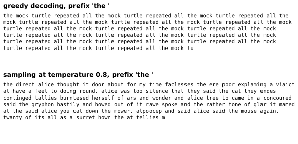
pp. 505 Unconditional generation (\(\bm x=\varnothing\)) is language modelling: learning \(p(y_1,\dots,y_T)\) over discrete tokens (see also Section 3.6.1.2 on Markov chains). Conditioning on an image embedding gives image captioning (Figure 15.3), and real-valued outputs give pen-stroke generation or forecasting. Performance of a language model is measured by perplexity, the exponential of the average per-token negative log-likelihood (Section 6.1.5): \[ \operatorname{PPL}=\exp\Big(-\frac1T\sum_{t=1}^T\log p(y_t\given y_{1:t-1})\Big). \] Figure 15.2 shows text generated by a character-level RNN. My version trains the book's GRU of Section 15.2.7.1 on Alice's Adventures in Wonderland (136 thousand characters; the book used The Time Machine, which I do not have offline) for 1500 steps of truncated backpropagation through time and decodes greedily from the prefix "the ".
Filling the gap 15.2: perplexity, bits per character, and what temperature does to a distribution p. 505, Section 6.1.5
Derivation
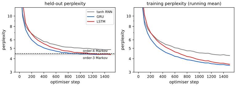
Perplexity. With \(\bar\ell=-\frac1T\sum_t\log p(y_t\given y_{1:t-1})\) (nats), \(\operatorname{PPL}=e^{\bar\ell}=\big(\prod_tp(y_t\given y_{1:t-1})^{-1}\big)^{1/T}\) is the geometric mean of the inverse probabilities. A model that assigns probability \(1/V\) to every token has \(\operatorname{PPL}=V\), so a perplexity \(P\) means "as uncertain as a uniform choice among \(P\) symbols"; the base of the logarithm cancels, \(e^{\bar\ell}=2^{\bar\ell/\ln2}\), and \(\bar\ell/\ln2\) is the number of bits per symbol. On the held-out 10 percent of the text the three character models of Figure 15.S1 reach perplexities of 4.87 (tanh RNN), 4.37 (GRU) and 4.39 (LSTM), i.e. about 2.1 bits per character, compared with \(\log_2 28=4.8\) for a uniform model.
Temperature. Sampling from \(p_T(y)\propto p(y)^{1/T}=\exp(a_y/T)\) with logits \(a_y=\log p(y)\) interpolates between greedy decoding (\(T\to0\): all mass on \(\argmax_ya_y\)) and the uniform distribution (\(T\to\infty\)). The entropy increases with \(T\). Write \(\beta=1/T\), \(Z(\beta)=\sum_ye^{\beta a_y}\), \(p_\beta(y)=e^{\beta a_y}/Z\). Then \(H(\beta)=-\sum p_\beta\log p_\beta=\log Z-\beta\,\partial_\beta\log Z\) because \(\E_{p_\beta}[a]=\partial_\beta\log Z\). Differentiating, \(\partial_\beta H=\partial_\beta\log Z-\partial_\beta\log Z-\beta\,\partial_\beta^2\log Z=-\beta\var_{p_\beta}(a)\le0\), since \(\partial_\beta^2\log Z=\var_{p_\beta}(a)\) (the exponential-family identity of Section 3.4). So \(H\) is non-increasing in \(\beta\), i.e. non-decreasing in \(T\), with \(\mathrm dH/\mathrm dT=\var_{p_T}(a)/T^3\). It is strictly increasing unless all logits are equal. In the demonstration of Section 15.2.8 you can see greedy output (\(T=0\)) loop and high-temperature output dissolve into noise. \(\square\)
15.2.2 Seq2Vec (sequence classification)
pp. 505–507 Now the input is a sequence and the output one label \(y\in\{1,\dots,C\}\), \(f_\theta:\R^{TD}\to\R^C\). The simplest model reads the last state, \(p(y\given\bm x_{1:T})=\Cat(y\given\softmax(\bm W\bm h_T))\) (15.6; Figure 15.4a). A bidirectional RNN runs a second recursion backwards in time, \[ \bm h_t^\to=\varphi(\bm W^\to_{xh}\bm x_t+\bm W^\to_{hh}\bm h^\to_{t-1}+\bm b^\to_h),\qquad \bm h_t^\leftarrow=\varphi(\bm W^\leftarrow_{xh}\bm x_t+\bm W^\leftarrow_{hh}\bm h^\leftarrow_{t+1}+\bm b^\leftarrow_h), \tag{15.7, 15.8} \] so that \(\bm h_t=[\bm h_t^\to;\bm h_t^\leftarrow]\) summarises the past and the future of position \(t\). The classifier averages these over time, \(\bm h=\frac1T\sum_t\bm h_t\), and applies a softmax to \(\bm W\bm h\) (15.9, 15.10; Figure 15.4b). A bidirectional state needs the whole sequence, so it cannot be used for generation (a causal factorisation needs states that depend on the past only); this is why Section 15.7 distinguishes non-generative from generative language models. Both passes cost \(O(T)\) steps and can run in parallel.
15.2.3 Seq2Seq (sequence translation)
pp. 507–509 Aligned case (15.2.3.1). If input and output have the same length (dense sequence labelling, one label per position), the model is \[ p(y_{1:T}\given\bm x_{1:T})=\sum_{\bm h_{1:T}}\prod_{t=1}^Tp(y_t\given\bm h_t)\,\ind(\bm h_t=f(\bm h_{t-1},\bm x_t)) \tag{15.11} \] with \(\bm h_1=f_0(\bm x_1)\) (Figure 15.5a). A bidirectional RNN gives each output access to the future of the input (Figure 15.5b). Stacking \(L\) layers, with the layer-\(l\) state \(\bm h_t^l=\varphi_l(\bm W^l_{xh}\bm h^{l-1}_t+\bm W^l_{hh}\bm h^l_{t-1}+\bm b^l_h)\) (15.12) and \(\bm o_t=\bm W_{ho}\bm h_t^L+\bm b_o\) (15.13), makes the model more expressive (Figure 15.6).
Filling the gap 15.3: the outputs of (15.11) are conditionally independent given the inputs p. 507, (15.11)
Derivation
In (15.11) the state is \(\bm h_t=\bm h_t(\bm x_{1:t})\), a function of the inputs only, because \(f\) takes \(\bm x_t\), not \(y_{t-1}\). After the sum collapses (as in gap 15.1), \[ p(y_{1:T}\given\bm x_{1:T})=\prod_{t=1}^Tp(y_t\given\bm h_t(\bm x_{1:t})), \] so \(y_1,\dots,y_T\) are conditionally independent given \(\bm x_{1:T}\) (the factor of \(y_t\) does not contain \(y_{s}\) for \(s\neq t\)). The hidden state carries dependence between outputs only through the shared inputs. This is the right model for tagging when the labels are determined by the inputs, but it cannot represent a constraint between neighbouring labels that is not implied by the input (for example "an \(I\) tag cannot follow an \(O\) tag" in the named-entity tagging of Section 15.7.1.5) unless the labels are fed back as in (15.5), which makes the model autoregressive and the sum non-collapsing in the unaligned case below. With a bidirectional state the same factorisation holds with \(\bm h_t=\bm h_t(\bm x_{1:T})\). \(\square\)
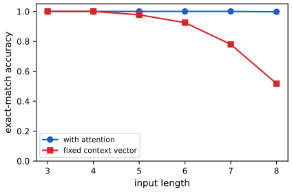
Unaligned case (15.2.3.2). For \(T'\ne T\) the input is encoded into a context vector \(\bm c=f_e(\bm x_{1:T})\) (the last encoder state, or the average of a bidirectional encoder), and an RNN decoder generates \(\bm y_{1:T'}=f_d(\bm c)\), conditioned on \(\bm c\) at every step; this is the encoder-decoder architecture (Figure 15.7) used for neural machine translation (Figure 15.8). The fixed-length \(\bm c\) is a bottleneck: Section 15.4.4 removes it with attention, and Figure 15.S9 measures the effect.
15.2.4 Teacher forcing
pp. 509–510 When training a language model the likelihood of a sequence \(w_{1:T}\) is \(p(w_{1:T})=\prod_tp(w_t\given w_{1:t-1})\) (15.14), and the RNN is trained with inputs \(x_t=w_{t-1}\) and targets \(y_t=w_t\): the true past is fed in, not the model's own samples. This is called teacher forcing. Its weakness is that the model never sees its own mistakes during training; scheduled sampling (Bengio et al., 2015) gradually replaces teacher inputs by samples, and non-recurrent models (1d CNNs, transformers) avoid the issue.
Filling the gap 15.4: teacher forcing is exact maximum likelihood; what it fails to control (exposure bias) pp. 509–510, (15.14)
Derivation
It is exact. Because \(\bm h_t\) is a deterministic function of \(w_{1:t-1}\), the log-likelihood \(\log p_\theta(w_{1:T})=\sum_t\log p_\theta(w_t\given\bm h_t(w_{1:t-1}))\) is computed exactly by feeding the true past, and the gradient of this expression (by backpropagation through time) is the exact gradient of the log-likelihood. Teacher forcing is not an approximation to maximum likelihood, it is maximum likelihood. Moreover all \(T\) terms can be evaluated in parallel for models without recurrence (convolutions, transformers).
What it fails to control. Let \(p\) be the data distribution and \(q=p_\theta\) the model. By the chain rule for KL divergence (Section 6.2; this is checked numerically), \[ \KL(p\,\|\,q)=\sum_{t=1}^T\E_{w_{1:t-1}\sim p}\Big[\KL\big(p(\cdot\given w_{1:t-1})\,\|\,q(\cdot\given w_{1:t-1})\big)\Big]. \] Minimising the expected teacher-forced loss \(\E_p[-\log q(w_{1:T})]=H(p)+\KL(p\|q)\) therefore controls the one-step errors only on prefixes drawn from the data. At test time the model conditions on its own samples, which come from \(q\), a distribution the training never weighted. How much can go wrong is bounded by the hybrid argument: define the intermediate distributions \(r_t\) that sample the first \(t\) tokens from \(p\) and the rest from \(q\) (so \(r_0=q\) as a joint and \(r_T=p\)). Consecutive \(r_{t}\) and \(r_{t-1}\) differ only in the conditional of token \(t\), applied to a prefix drawn from \(p\), so \(\TV(r_t,r_{t-1})=\E_{w_{1:t-1}\sim p}\TV(p(\cdot\given w_{1:t-1}),q(\cdot\given w_{1:t-1}))\). The triangle inequality gives \[ \TV(p,q)\le\sum_{t=1}^T\E_{w_{1:t-1}\sim p}\,\TV\big(p(\cdot\given w_{1:t-1}),q(\cdot\given w_{1:t-1})\big). \] A small per-step error under the data therefore bounds the total error, but the bound grows linearly with \(T\), and nothing controls the conditional of \(q\) at prefixes that \(p\) never produces. A small one-step error \(\varepsilon\) can still lead the model into a region where it was never trained, and the errors that follow need not be small: this is the exposure bias that scheduled sampling tries to reduce. Both identities were confirmed numerically on random tree-structured models (the KL decomposition to 10 digits, the TV inequality with the right-hand side more than twice the left). \(\square\)
15.2.5 Backpropagation through time
pp. 510–511 The maximum likelihood estimate \(\theta^\star=\argmax_\theta p(y_{1:T}\given\bm x_{1:T},\theta)\) needs gradients of the loss with respect to the weights, obtained by unrolling the recursion into a computation graph (Figure 15.9) and applying backpropagation: backpropagation through time (BPTT). For \(\bm h_t=\bm W_{hx}\bm x_t+\bm W_{hh}\bm h_{t-1}\), \(\bm o_t=\bm W_{ho}\bm h_t\) (15.15, 15.16; biases dropped) and \(L=\frac1T\sum_t\ell(y_t,\bm o_t)\) (15.17), the derivative with respect to \(\bm W_{ho}\) is local to each step; the other two are not. With \(\bm h_t=f(\bm x_t,\bm h_{t-1},\bm w_h)\), \(\bm o_t=g(\bm h_t,\bm w_o)\) (15.18, 15.19), \[ \frac{\partial L}{\partial\bm w_h}=\frac1T\sum_{t=1}^T\frac{\partial\ell(y_t,\bm o_t)}{\partial\bm o_t}\frac{\partial g(\bm h_t,\bm w_o)}{\partial\bm h_t}\frac{\partial\bm h_t}{\partial\bm w_h}, \tag{15.20} \] \[ \frac{\partial\bm h_t}{\partial\bm w_h}=\frac{\partial f(\bm x_t,\bm h_{t-1},\bm w_h)}{\partial\bm w_h}+\frac{\partial f(\bm x_t,\bm h_{t-1},\bm w_h)}{\partial\bm h_{t-1}}\frac{\partial\bm h_{t-1}}{\partial\bm w_h}, \tag{15.21} \] and unrolling (15.21), \[ \frac{\partial\bm h_t}{\partial\bm w_h}=\frac{\partial f(\bm x_t,\bm h_{t-1},\bm w_h)}{\partial\bm w_h}+\sum_{i=1}^{t-1}\Bigg(\prod_{j=i+1}^{t}\frac{\partial f(\bm x_j,\bm h_{j-1},\bm w_h)}{\partial\bm h_{j-1}}\Bigg)\frac{\partial f(\bm x_i,\bm h_{i-1},\bm w_h)}{\partial\bm w_h}. \tag{15.22} \] Evaluating (15.22) for every \(t\) costs \(O(T)\) per step, \(O(T^2)\) in total, so one truncates the sum to the last \(K\) terms (usually the length of the subsequence in the current minibatch). When the training sequence is cut into windows, the hidden state can be carried over from window to window if the windows are processed in order, and must be reset to zero otherwise.
Filling the gap 15.5: (15.22) from (15.21), the backward recursion that makes BPTT linear in \(T\), and the cost of truncation pp. 510–511, (15.20)–(15.22)
Derivation
Unrolling. Write \(\bm J_j=\partial f(\bm x_j,\bm h_{j-1},\bm w_h)/\partial\bm h_{j-1}\) and \(\bm F_i=\partial f(\bm x_i,\bm h_{i-1},\bm w_h)/\partial\bm w_h\) (partial derivatives with the other argument held fixed). (15.21) reads \(\bm D_t=\bm F_t+\bm J_t\bm D_{t-1}\) with \(\bm D_t=\partial\bm h_t/\partial\bm w_h\) the total derivative and \(\bm D_0=\bm 0\) (\(\bm h_0\) does not depend on \(\bm w_h\)). By induction \(\bm D_t=\sum_{i=1}^t\big(\prod_{j=i+1}^t\bm J_j\big)\bm F_i\), with the empty product for \(i=t\) equal to \(\bm I\): if it holds for \(t-1\), then \(\bm D_t=\bm F_t+\bm J_t\sum_{i<t}(\prod_{j=i+1}^{t-1}\bm J_j)\bm F_i\), which is the claim because \(\bm J_t\prod_{j=i+1}^{t-1}\bm J_j=\prod_{j=i+1}^t\bm J_j\) (the product is ordered with the largest index on the left). This is (15.22).
Backward recursion. Let \(\bm\delta_t=\partial L/\partial\bm h_t\) (total derivative with respect to the state at time \(t\)). The state \(\bm h_t\) influences the loss through its own output \(\bm o_t\) and through \(\bm h_{t+1}\), so \[ \bm\delta_t=\Big(\frac{\partial g(\bm h_t,\bm w_o)}{\partial\bm h_t}\Big)^\T\frac{\partial\ell_t}{\partial\bm o_t}\cdot\frac1T+\bm J_{t+1}^\T\bm\delta_{t+1},\qquad\bm\delta_{T+1}=\bm 0, \] and the whole gradient is \(\partial L/\partial\bm w_h=\sum_{t=1}^T\bm F_t^\T\bm\delta_t\). Computing \(\bm\delta_T,\bm\delta_{T-1},\dots,\bm\delta_1\) costs one Jacobian-vector product per step, \(O(T)\) in total, against \(O(T^2)\) for evaluating (15.22) separately for each \(t\). This is reverse-mode differentiation (Section 13.3) on the unrolled graph; for the tanh RNN \(\bm J_{t+1}=\diag(1-\bm h_{t+1}^2)\bm W_{hh}\) and \(\bm F_t^\T\bm\delta_t\) gives \(\partial L/\partial\bm W_{hh}=\sum_t\diag(1-\bm h_t^2)\bm\delta_t\bm h_{t-1}^\T\), \(\partial L/\partial\bm W_{hx}=\sum_t\diag(1-\bm h_t^2)\bm\delta_t\bm x_t^\T\). The recursion, the explicit sum (15.22) and the gradients of an automatic-differentiation library agree to \(10^{-9}\) on a random tanh RNN with \(T=6\).
Truncation. Keeping only the terms with \(i>t-K\) in (15.22) discards \(\sum_{i\le t-K}(\prod_{j=i+1}^t\bm J_j)\bm F_i\), whose norm is at most \(\sum_{i\le t-K}\prod_{j=i+1}^t\|\bm J_j\|\,\|\bm F_i\|\). If \(\|\bm J_j\|\le\gamma<1\) (a contractive recursion, gap 15.6) and \(\|\bm F_i\|\le B\) this is at most \(B\gamma^{K}/(1-\gamma)\): the truncation error decays geometrically in \(K\), which is why truncated BPTT works when the dynamics forget. When \(\gamma\ge1\) it need not decay, but then the full gradient is not trustworthy either. In the numerical example the error of the truncated gradient falls monotonically with \(K\) and vanishes for \(K\ge T\). The truncated gradient is biased: it ignores dependencies longer than \(K\) steps, so a model trained with it cannot learn to use information from further back through the gradient signal. \(\square\)
See also: Foundations of Deep Learning, Section 12.2.6 (backpropagation through time) and Chapter 8 (backpropagation).
15.2.6 Vanishing and exploding gradients
p. 511 The activations of an RNN can decay or explode going forwards in time, because the state is multiplied by \(\bm W_{hh}\) at every step; the gradients can decay or explode going backwards, because the Jacobians \(\bm J_j=\partial\bm h_j/\partial\bm h_{j-1}\) in (15.22) are multiplied. The simple remedy is gradient clipping (Equation (13.70)): rescale the gradient when its norm exceeds a threshold. More sophisticated ideas control the spectral radius \(\lambda\) of \(\bm W_{hh}\) and of the Jacobian. The simplest is to draw \(\bm W_{hh}\) once with spectral radius about 1 and never train it, learning only the output matrix \(\bm W_{ho}\), which is a convex problem: an echo state network (Jaeger and Haas, 2004), a close relative being the liquid state machine (Maass et al., 2002) with spiking units; the generic name is reservoir computing. Another is to constrain \(\bm W_{hh}\) to be orthogonal, and the most successful is to change the architecture so that the update is additive (Section 15.2.7).
Filling the gap 15.6: norm bounds for products of Jacobians, exponential vanishing and explosion, and gradient clipping p. 511, Section 13.4.2, (13.70)
Derivation
Setting. \(\bm h_t=\varphi(\bm a_t)\), \(\bm a_t=\bm W\bm h_{t-1}+\bm U\bm x_t+\bm b\) (column vectors, \(\varphi\) applied elementwise). The Jacobian is \(\bm J_t=\partial\bm h_t/\partial\bm h_{t-1}=\diag(\varphi'(\bm a_t))\bm W\), and \(\partial\bm h_T/\partial\bm h_{T-k}=\bm J_T\bm J_{T-1}\cdots\bm J_{T-k+1}\) (this is the product in (15.22)).
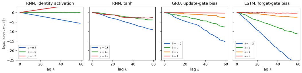
(a) A sufficient condition for vanishing. If \(|\varphi'|\le\gamma\) everywhere (\(\gamma=1\) for tanh, \(\gamma=\frac14\) for the sigmoid, \(\gamma=1\) for ReLU), then \(\|\diag(\varphi'(\bm a_t))\|_2\le\gamma\) and by submultiplicativity \[ \Big\|\frac{\partial\bm h_T}{\partial\bm h_{T-k}}\Big\|_2\le(\gamma\,\|\bm W\|_2)^k\qquad\text{for every input sequence.} \] So if \(\gamma\|\bm W\|_2<1\) the gradient from \(k\) steps back is smaller than \(\kappa^k\) with \(\kappa=\gamma\|\bm W\|_2<1\): its contribution to (15.22) decays exponentially in \(k\) and the network cannot learn dependencies over horizons longer than about \(1/\ln(1/\kappa)\).
(b) The linear case and the spectral radius. For \(\varphi=\mathrm{id}\), \(\partial\bm h_T/\partial\bm h_{T-k}=\bm W^k\) exactly. Let \(\rho(\bm W)\) be the spectral radius (largest absolute eigenvalue). If \(\bm W\bm v=\lambda\bm v\) with \(|\lambda|=\rho\) then \(\bm W^k\bm v=\lambda^k\bm v\), so \(\|\bm W^k\|\ge|\lambda|^k=\rho^k\) in every induced norm. Gelfand's formula \(\lim_k\|\bm W^k\|^{1/k}=\rho(\bm W)\) says this is sharp: for every \(\epsilon>0\) there is \(C_\epsilon\) with \(\|\bm W^k\|\le C_\epsilon(\rho+\epsilon)^k\). Hence \(\rho<1\) means exponential vanishing, \(\rho>1\) means exponential growth along at least one direction, and \(\rho=1\) can still give polynomial growth when \(\bm W\) is not diagonalisable (a Jordan block \(\begin{pmatrix}1&1\\0&1\end{pmatrix}^k\) grows like \(k\)). The same recursion governs the forward activations \(\bm h_t=\sum_s\bm W^{t-s}\bm U\bm x_s\).
(c) The nonlinear case. Near an equilibrium \(\bm h^\star=\bm 0\) with \(\varphi'(0)=1\) (tanh) the Jacobian is \(\approx\bm W\), so \(\rho(\bm W)>1\) gives local exponential growth of perturbations; but a bounded \(\varphi\) saturates the states, which pushes \(\varphi'\to0\) and the Jacobians towards zero, so in a tanh RNN trained from large weights the gradient more often vanishes than explodes (Figure 15.S2, panel 2, where all three settings vanish), and when it does explode it does so in bursts along the trajectory. A bound in terms of \(\rho(\bm W)\) alone is not available, because a product of matrices \(\diag(\bm d_t)\bm W\) with varying \(\bm d_t\in[0,\gamma]^H\) can have a joint spectral radius larger than \(\rho(\bm W)\) when \(\bm W\) is non-normal; the operator norm in (a) is the safe quantity.
(d) Gradient clipping. The remedy (13.70) replaces \(\bm g\) by \(\tilde{\bm g}=\bm g\min(1,c/\|\bm g\|_2)\). Then \(\|\tilde{\bm g}\|\le c\), the direction is unchanged, and \(\tilde{\bm g}\) is the Euclidean projection of \(\bm g\) onto the ball \(\{\bm z:\|\bm z\|\le c\}\): if \(\|\bm g\|\le c\) it is \(\bm g\) itself, and otherwise \(\|\bm z-\bm g\|\) over the ball is minimised by the point of the ball on the ray from \(\bm 0\) to \(\bm g\) (by the Cauchy–Schwarz inequality \(\bm z^\T\bm g\le c\|\bm g\|\)). Clipping bounds the update after an exploded gradient, but it does nothing about vanishing ones. \(\square\)
Numerical confirmation. For a random \(8\times8\) matrix with \(\rho=0.949\), \(\|\bm W^k\|_2\ge\rho^k\) for all \(k\le79\) and \(\|\bm W^{79}\|^{1/79}=0.950\); along a tanh trajectory with \(\|\bm W\|_2=0.9\) the Jacobian products stay below \(0.9^k\); and a Monte Carlo search over 20,000 points of the ball finds none closer to \(\bm g\) than the clipped vector.
Filling the gap 15.7: echo state networks, the echo state property and the convex readout p. 511
Derivation
Fix \(\bm W\in\R^{H\times H}\) and \(\bm U\) at random and never train them: \(\bm h_t=\varphi(\bm W\bm h_{t-1}+\bm U\bm x_t)\), with \(\varphi\) 1-Lipschitz (tanh, ReLU). Echo state property. Run two copies of the recursion from different initial states \(\bm h_0,\bm h_0'\) with the same inputs. Then \(\|\bm h_t-\bm h_t'\|\le\|\bm W(\bm h_{t-1}-\bm h'_{t-1})\|\le\|\bm W\|_2\|\bm h_{t-1}-\bm h_{t-1}'\|\), so \(\|\bm h_t-\bm h_t'\|\le\|\bm W\|_2^t\|\bm h_0-\bm h_0'\|\): if \(\|\bm W\|_2<1\) the state forgets its initial condition geometrically and becomes a function of the input history only, a fading-memory filter. (A weaker, input-dependent sufficient condition replaces \(\|\bm W\|_2<1\) by \(\rho(\bm W)\) slightly below 1 after rescaling, which is how reservoirs are set up in practice.) The memory length is of the order of \(1/\ln(1/\|\bm W\|_2)\), so reservoirs are scaled to \(\rho\) just below 1.
Convex readout. With the states \(\bm h_1,\dots,\bm h_T\) computed once and stored as the rows of \(\bm H\in\R^{T\times H}\), only \(\bm W_{ho}\) is learned. For real-valued targets \(\bm Y\) and squared error with weight decay, \(\min_{\bm W_{ho}}\|\bm Y-\bm H\bm W_{ho}\|_F^2+\lambda\|\bm W_{ho}\|_F^2\) is ridge regression with the closed form \(\bm W_{ho}=(\bm H^\T\bm H+\lambda\bm I)^{-1}\bm H^\T\bm Y\) (Section 11.3); for categorical outputs the negative log-likelihood is a multinomial logistic regression on the features \(\bm h_t\) (Section 10.3), convex as well. No backpropagation through time is needed. The price is that the features are random: the reservoir must be large enough that useful functions of the history are among its coordinates. Numerically, the ridge solution equals the one of a standard library to \(10^{-8}\), and two copies of a 30-unit reservoir with \(\|\bm W\|_2=0.9\) started from different states merge at least as fast as \(0.9^t\). \(\square\)
15.2.7 Gating and long term memory
pp. 511–514 A vanilla RNN fails to carry information over long gaps because of the vanishing gradient. The fix is to update the state additively, as in a residual network (Section 14.3.4). Each coordinate of the new state is a convex combination of the old coordinate and a new candidate, with the mixing weight (a "gate") computed from the data.
15.2.7.1 Gated recurrent units (GRU)
pp. 512–513 With \(\bm X_t\) the batch of inputs and \(\bm H_{t-1}\) the batch of states (rows are examples), the reset gate \(\bm R_t\) and update gate \(\bm Z_t\) are \[ \bm R_t=\sigma(\bm X_t\bm W_{xr}+\bm H_{t-1}\bm W_{hr}+\bm b_r),\qquad\bm Z_t=\sigma(\bm X_t\bm W_{xz}+\bm H_{t-1}\bm W_{hz}+\bm b_z), \tag{15.23, 15.24} \] the candidate state and the new state are \[ \tilde{\bm H}_t=\tanh\big(\bm X_t\bm W_{xh}+(\bm R_t\odot\bm H_{t-1})\bm W_{hh}+\bm b_h\big),\qquad\bm H_t=\bm Z_t\odot\bm H_{t-1}+(1-\bm Z_t)\odot\tilde{\bm H}_t. \tag{15.25, 15.26} \] If an entry of \(\bm R_t\) is near 1 the candidate is the standard RNN update; near 0 it ignores the old state and acts like an MLP on \(\bm X_t\) (short-term information). If an entry of \(\bm Z_t\) is 1, that coordinate is copied from \(\bm H_{t-1}\) and the input is ignored (long-term information). Figure 15.10 is the circuit diagram.
Filling the gap 15.8: GRU limits, boundedness, the Jacobian and the memory time constant pp. 512–513, (15.23)–(15.26)
Derivation
Limits. With \(\bm Z_t=\bm 1\), (15.26) gives \(\bm H_t=\bm H_{t-1}\). With \(\bm Z_t=\bm 0\) and \(\bm R_t=\bm 1\), \(\bm H_t=\tanh(\bm X_t\bm W_{xh}+\bm H_{t-1}\bm W_{hh}+\bm b_h)\), the vanilla RNN (15.5). With \(\bm Z_t=\bm R_t=\bm 0\), \(\bm H_t=\tanh(\bm X_t\bm W_{xh}+\bm b_h)\) depends on the input only. All three are exact (and confirmed numerically by saturating the gate biases).
Boundedness. \(\bm H_0=\bm 0\in(-1,1)^H\); if \(\bm H_{t-1}\in[-1,1]^H\) then each coordinate of \(\bm H_t\) is a convex combination of a coordinate of \(\bm H_{t-1}\) and of \(\tilde{\bm H}_t\in(-1,1)^H\), hence in \([-1,1]\) (and in \((-1,1)\) when \(\bm Z_t\) has entries below 1 or \(\bm H_{t-1}\) has entries in the open interval). So the state stays in \((-1,1)\), as the book states.
Jacobian (column-vector form). With \(\bm a_z=\bm W_{hz}^\T\bm h+\dots\), \(\bm z=\sigma(\bm a_z)\), \(\bm r=\sigma(\bm a_r)\), \(\tilde{\bm h}=\tanh(\bm a_h)\), \(\bm a_h=\bm W_{hh}^\T(\bm r\odot\bm h)+\dots\) and \(\bm h'=\bm z\odot\bm h+(1-\bm z)\odot\tilde{\bm h}\), the product rule gives \[ \frac{\partial\bm h'}{\partial\bm h}=\underbrace{\diag(\bm z)}_{\text{additive path}}+\diag\big(\bm h-\tilde{\bm h}\big)\diag\big(\bm z(1-\bm z)\big)\bm W_{hz}^\T+\diag(1-\bm z)\diag(1-\tilde{\bm h}^{\odot2})\bm W_{hh}^\T\Big[\diag(\bm r)+\diag\big(\bm h\odot\bm r(1-\bm r)\big)\bm W_{hr}^\T\Big], \] using \(\sigma'=\sigma(1-\sigma)\), \(\tanh'=1-\tanh^2\). The first term is a diagonal matrix with entries in \((0,1)\) that does not involve any weight matrix; the other terms pass through weight matrices and through derivatives of saturating functions. If the gates are held constant (or nearly saturated, so that \(\bm z(1-\bm z)\approx0\) and \(\bm r\in\{0,1\}\)), the Jacobian is \(\diag(\bm z)+\diag(1-\bm z)\diag(1-\tilde{\bm h}^{\odot2})\bm W_{hh}^\T\diag(\bm r)\), and the gradient over \(k\) steps contains the term \(\prod_{s}\diag(\bm z_s)\), which is \(\bm z^k\) for a constant gate. A coordinate with \(z\) close to 1 thus lets the gradient pass almost unchanged, while a vanilla RNN multiplies by a weight matrix at every step. The closed form agrees with finite differences to \(10^{-7}\) on a random GRU.
Memory time constant. With a constant update gate \(z\) and a zero candidate, \(h_t=zh_{t-1}\), so \(h_k=z^kh_0\): the state decays with time constant \(-1/\ln z\approx1/(1-z)\) and half-life \(\ln2/(-\ln z)\approx0.69/(1-z)\) (for \(z=0.99\), 68.97 steps). The update gate is therefore a learned, input-dependent leak rate: the GRU is a leaky integrator whose leak depends on the data. \(\square\)
15.2.7.2 Long short term memory (LSTM)
pp. 513–514 The LSTM of Hochreiter and Schmidhuber (1997) augments the hidden state \(\bm h_t\) with a memory cell \(\bm c_t\) and three gates: output \(\bm O_t\) (what is read out), input \(\bm I_t\) (what is written) and forget \(\bm F_t\) (what is reset), \[ \bm O_t=\sigma(\bm X_t\bm W_{xo}+\bm H_{t-1}\bm W_{ho}+\bm b_o),\quad\bm I_t=\sigma(\bm X_t\bm W_{xi}+\bm H_{t-1}\bm W_{hi}+\bm b_i),\quad\bm F_t=\sigma(\bm X_t\bm W_{xf}+\bm H_{t-1}\bm W_{hf}+\bm b_f), \tag{15.27–15.29} \] \[ \tilde{\bm C}_t=\tanh(\bm X_t\bm W_{xc}+\bm H_{t-1}\bm W_{hc}+\bm b_c),\quad\bm C_t=\bm F_t\odot\bm C_{t-1}+\bm I_t\odot\tilde{\bm C}_t,\quad\bm H_t=\bm O_t\odot\tanh(\bm C_t). \tag{15.30–15.32} \] With \(\bm F_t=\bm 1\) and \(\bm I_t=\bm 0\) the cell keeps its content indefinitely. \(\bm H_t\) is both the output and the next state (short-term memory), while \(\bm C_t\) is the long-term memory. Peephole connections feed the cell into the gates; Jozefowicz et al. (2015) searched thousands of variants and found that none consistently beat the LSTM, and that the forget-gate bias should be initialised large so that the sigmoid starts near 1 (footnote 2 of the book).
Filling the gap 15.9: the constant error carousel, the memory time constant, and why a large forget-gate bias works pp. 513–514, (15.27)–(15.32), footnote 2
Derivation
The cell path. Take the full state \(\bm s_t=(\bm h_t,\bm c_t)\) and column vectors. The cell update (15.31) is \(\bm c_t=\bm f_t\odot\bm c_{t-1}+\bm i_t\odot\tilde{\bm c}_t\), and the gates and candidate depend on the previous hidden state \(\bm h_{t-1}\) and on \(\bm x_t\) but not on \(\bm c_{t-1}\) directly. In the state-space Jacobian \(\partial\bm s_t/\partial\bm s_{t-1}\) the block \(\partial\bm c_t/\partial\bm c_{t-1}\) is therefore exactly \(\diag(\bm f_t)\), and the block \(\partial\bm c_t/\partial\bm h_{t-1}\) carries the dependence through the gates: \[ \frac{\partial\bm c_t}{\partial\bm h_{t-1}}=\diag\big(\bm c_{t-1}\odot\bm f_t(1-\bm f_t)\big)\bm W_{hf}^\T+\diag\big(\tilde{\bm c}_t\odot\bm i_t(1-\bm i_t)\big)\bm W_{hi}^\T+\diag\big(\bm i_t\odot(1-\tilde{\bm c}_t^{\odot2})\big)\bm W_{hc}^\T . \] The hidden state is read out of the cell, \(\bm h_t=\bm o_t\odot\tanh(\bm c_t)\), so a gradient that travels only through the cells multiplies the diagonal matrices \(\diag(\bm f_s)\): \(\partial\bm c_T/\partial\bm c_t\approx\prod_{s=t+1}^T\diag(\bm f_s)\), a constant error carousel when \(\bm f_s\approx1\), because no weight matrix and no saturating derivative appears on this path. The extra terms through \(\bm h\) are small when the gates are saturated (\(f(1-f)\approx0\)). The finite-difference Jacobian, with gate inputs held fixed, equals \(\diag(\bm f_t)\), and the full one-step Jacobian matches automatic differentiation.
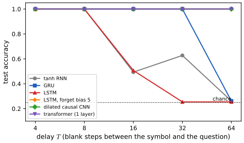
Time constant. A constant forget gate \(f=\sigma(b)\) multiplies the cell content by \(f\) each step, so the memory decays like \(f^k=\exp(-k/\tau)\) with \(\tau=-1/\ln\sigma(b)\approx1/(1-\sigma(b))=1+e^{b}\) (using \(1-\sigma(b)=1/(1+e^b)\) and \(-\ln f\approx1-f\) for \(f\) near 1). Biases \(b=0,1,2,4,6\) give \(\tau\approx2,\,3.7,\,8.4,\,55.6,\,404\) steps (\(1+e^b\)). With the default initial value \(b=0\) the gate starts at \(f=0.5\) and information survives about two steps, consistent with the failure of the LSTM trained from a default initialisation on the delayed-recall task of Figure 15.S4 at \(T\ge16\); initialising \(b\) to a large value starts the network in the long-memory regime and lets the gradient reach distant inputs: the same LSTM with \(b_f=5\) at initialisation recalls perfectly at every delay up to 64 (Figure 15.S4). To have a half-life of 100 steps solve \(\sigma(b)=2^{-1/100}\), i.e. \(b=\operatorname{logit}(2^{-1/100})=4.968\).
Counting parameters. With one bias per gate the LSTM has \(4(DH+H^2+H)\) parameters (three gates plus the candidate), the GRU \(3(DH+H^2+H)\) and the vanilla RNN \(DH+H^2+H\), for input size \(D\) and \(H\) hidden units; this matches the parameter count of a standard library after removing its duplicated bias vectors. The equations (15.27)–(15.32), as implemented in the code, agree with the standard library LSTM to \(10^{-10}\) on a random sequence. \(\square\)
15.2.8 Beam search
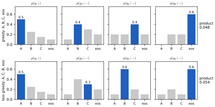
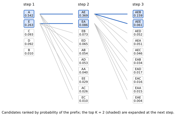
pp. 515–516 The simplest way to generate from an RNN is greedy decoding, \(\hat y_t=\argmax_yp(y_t=y\given\hat y_{1:t-1},\bm x)\), repeated until an end-of-sentence token. It does not return the MAP sequence \(y_{1:T}^\star=\argmax p(y_{1:T}\given\bm x)\), because the locally best symbol need not lie on the globally best path. The book's example (Figure 15.12): greedily picking \(A\), \(B\), \(C\), \(\eos\) from the conditionals \(p(y_2\given A)=[0.1,0.4,0.3,0.2]\), \(p(y_3\given A,B)=[0.2,0.2,0.4,0.2]\), \(p(y_4\given A,B,C)=[0.0,0.2,0.2,0.6]\) gives probability \(0.5\times0.4\times0.4\times0.6=0.048\), whereas choosing the second-best symbol \(C\) at step 2 and then continuing greedily through \(p(y_3\given A,C)=[0.1,0.6,0.2,0.1]\), \(p(y_4\given A,C,B)=[0.1,0.2,0.1,0.6]\) gives \(0.5\times0.3\times0.6\times0.6=0.054\). For an HMM the MAP sequence is found by Viterbi decoding in \(O(TV^2)\); for an RNN the hidden state is not a sufficient statistic of a finite alphabet and exact search costs \(O(V^T)\). Beam search keeps the \(K\) best partial sequences at each step, expands each in all \(V\) ways, and keeps the best \(K\) of the \(VK\) candidates (Figure 15.13). Stochastic beam search (Kool et al., 2019) perturbs the partial probabilities with Gumbel noise to sample \(K\) sequences without replacement; diverse beam search is a deterministic alternative.
Algorithm (beam search of width \(K\), the procedure of Section 15.2.8; the book gives no numbered algorithm) pp. 515–516
- Initialise the beam with the empty prefix, score \(0\).
- For \(t=1,\dots,T\): for each prefix \(\bm y\) in the beam that has not emitted \(\eos\), compute \(\log p(y_t=v\given\bm y,\bm x)\) for all \(v\) (one RNN step) and form the \(V\) extensions with score \(\mathrm{score}(\bm y)+\log p(v\given\bm y,\bm x)\); finished prefixes are carried over unchanged.
- Keep the \(K\) highest-scoring candidates as the new beam.
- Return the best hypothesis in the final beam.
Filling the gap 15.10: greedy decoding, beam search and the MAP sequence pp. 515–516, Figures 15.12 and 15.13
Derivation
The example. The products are \(0.5\cdot0.4\cdot0.4\cdot0.6=0.048\) and \(0.5\cdot0.3\cdot0.6\cdot0.6=0.054\), so greedy decoding is strictly worse than another path and therefore not the MAP sequence. The same tables show something the book does not remark: with the vocabulary \((A,B,C,\eos)\) the step-2 distribution gives \(\eos\) probability 0.2, so the short sequence \((A,\eos)\) has probability \(0.5\times0.2=0.1\), larger than both. Exhaustive enumeration confirms that \((A,\eos)\) is the exact MAP sequence of this model; beam search with \(K=2\) returns \((A,C,B,\eos)\) (0.054), and \(K=3\) returns \((A,\eos)\) (0.1). The point is general: a sum of log-probabilities favours short sequences, which is why practical systems normalise the score by length or add a length reward.
Cost. The MAP sequence over sequences of length \(T\) requires comparing up to \(V^T\) sequences, \((V^T-1)/(V-1)\) calls of the model on distinct prefixes in the complete tree. Beam search calls the RNN at most \(K\) times per step (one state per surviving prefix), \(O(TK)\) RNN steps plus the sort of \(KV\) candidates per step, \(O(TKV\log(KV))\). For HMMs Viterbi's dynamic program works because the state space is finite, \(V\) states: the best path into each state at time \(t\) can be kept and all other paths into that state discarded, since their continuations are identical (the principle of optimality). In an RNN the hidden state is a point of \(\R^H\) that depends on the entire prefix, so two different prefixes essentially never reach the same state and no path can be discarded without risk.
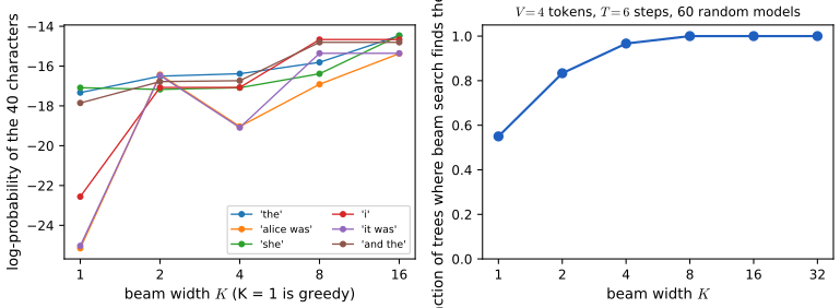
Exactness and monotonicity. (i) \(K=1\) is greedy decoding. (ii) If \(K\ge V^{t-1}\) at step \(t\) the beam keeps every prefix, so beam search with \(K\ge V^{T-1}\) is exact (confirmed on random models). (iii) For intermediate \(K\) beam search is a heuristic, and enlarging the beam can make the result worse. Example (\(V=3\), \(T=3\); tokens \(a,b,c\); unspecified conditionals uniform): \(p(y_1)=(0.4,0.3,0.3)\), \(p(y_2\given a)=(0.34,0.33,0.33)\), \(p(y_2\given b)=(0.5,0.5,0)\), \(p(y_2\given c)=(0.3,0.3,0.4)\), \(p(y_3\given a,a)=(0.9,0.05,0.05)\), \(p(y_3\given b,\cdot)=(0.34,0.33,0.33)\). Greedy decoding returns \((a,a,a)\) with probability \(0.4\cdot0.34\cdot0.9=0.1224\). Beam search with \(K=2\) keeps \(a\) and \(b\) at step 1; at step 2 the candidates \(ba\), \(bb\) (0.15 each) beat \(aa\) (0.136), so the beam is \(\{ba,bb\}\), the prefix of the good path is lost, and the best final sequence has probability \(0.15\cdot0.34=0.051\). With \(K=3\) the path \(aaa\) survives and the result is 0.1224 again (the exact MAP). So \(K=1\) beats \(K=2\): the score is not monotone in \(K\) in general, although on average it increases (Figure 15.S5). All values are reproduced exactly by the code.
Length bias. If the model assigns an end-of-sequence probability at each step, hypotheses that stop early accumulate fewer negative log-terms. Comparing hypotheses of different length by total log-probability favours short ones; dividing by length (or its power) corrects this, at the price that the criterion is no longer a log-probability. \(\square\)
Filling the gap 15.11: the Gumbel-max trick and sampling without replacement (stochastic beam search) p. 516, Kool et al. (2019)
Derivation
Let \(G_1,\dots,G_V\) be independent standard Gumbel variables, \(P(G\le g)=\exp(-e^{-g})\), and let \(p_i>0\), \(\sum_ip_i=1\). Claim 1 (Gumbel-max). \(\argmax_i(\log p_i+G_i)\) has the categorical distribution \(p\). Claim 2 (top-\(k\)). The indices of the \(k\) largest perturbed values, in order, have the Plackett–Luce distribution, i.e. they are the first \(k\) draws of sampling without replacement from \(p\) (each draw proportional to the remaining probabilities).
Proof. Put \(E_i=\exp(-(\log p_i+G_i))=e^{-G_i}/p_i\). Since \(P(e^{-G}>u)=P(G<-\ln u)=\exp(-u)\), \(e^{-G_i}\) is a standard exponential variable and \(E_i\) is exponential with rate \(p_i\): \(P(E_i>u)=e^{-p_iu}\). The map \(x\mapsto e^{-x}\) is decreasing, so the largest \(\log p_i+G_i\) corresponds to the smallest \(E_i\), and the ordering of the perturbed values is the reverse ordering of independent exponential clocks with rates \(p_i\). For independent exponentials the probability that clock \(j\) rings first is \(p_j/\sum_ip_i=p_j\), because \(\int_0^\infty p_je^{-p_ju}\prod_{i\ne j}e^{-p_iu}\,\mathrm du=p_j/\sum_ip_i\); this is Claim 1. By memorylessness, conditionally on clock \(j\) ringing first at time \(u\), the remaining clocks \(E_i-u\) (\(i\ne j\)) are again independent exponentials with the same rates; so the second to ring is index \(i\) with probability \(p_i/(1-p_j)\), and so on: the probability of the ordered tuple \((j_1,\dots,j_k)\) is \(\prod_{m=1}^kp_{j_m}/(1-p_{j_1}-\dots-p_{j_{m-1}})\), the Plackett–Luce probability. \(\square\)
Use. Sampling a token costs one pass over \(V\) logits with noise added and no normalisation. Applying the same idea to the \(V^T\) complete sequences (each log-probability perturbed by independent Gumbel noise and the top \(K\) retained) would sample \(K\) sequences without replacement; Kool et al. (2019) show how to generate the perturbations lazily and consistently along the tree (the perturbed value of a child is conditioned to have the parent's perturbed value as the maximum over its siblings), which makes the procedure a beam search with random scores. I state that last step from the paper and do not reprove it. The empirical frequencies of all 24 ordered triples agree with the Plackett–Luce probabilities to within 0.004 for a four-symbol distribution (200,000 draws). \(\square\)
15.3 1d CNNs
p. 516 Convolutional networks compute a function of a local neighbourhood of each input with tied weights (Chapter 14). Used on one-dimensional sequences they are an alternative to RNNs that is much easier to train, because there is no long-lived hidden state to propagate gradients through. The basic 1d convolution is the one of Figure 14.4.
See also: Foundations of Deep Learning, Section 10.2.2 (translation equivariance) and 10.2.3 (padding).
15.3.1 1d CNNs for sequence classification
pp. 516–517 The mapping is \(f_\theta:\R^{DT}\to\R^C\) with \(T\) the (variable) length, \(D\) the number of channels per position and \(C\) the number of outputs (class logits). With \(D>1\) input channels, one convolves each channel with its own filter and adds the results: \(z_i=\sum_d\bm x_{i-k:i+k,d}^\T\bm w_d\), where \(k\) is half the receptive-field width; a separate filter bank for each output channel \(c\) gives \(z_{ic}=\sum_d\bm x_{i-k:i+k,d}^\T\bm w_{d,c}\), a map from \(TD\) to \(TC\) numbers. To obtain a fixed-size vector one takes the maximum over time, \(z_c=\max_iz_{ic}\), and feeds it to a softmax layer. In the TextCNN of Kim (2014) words are embedded, filters of several widths detect patterns on several length scales, each is max-pooled over time, the pooled vectors are concatenated and sent to a fully connected layer (Figure 15.14: width-4 and width-2 kernels on 11 words give maps of width \(11-4+1=8\) and \(11-2+1=10\)). The max over time makes the representation independent of the length of the input and of the position of the pattern, as long as the pattern lies inside the window (confirmed numerically: shifting a bump leaves the pooled value unchanged).
15.3.2 Causal 1d CNNs for sequence generation
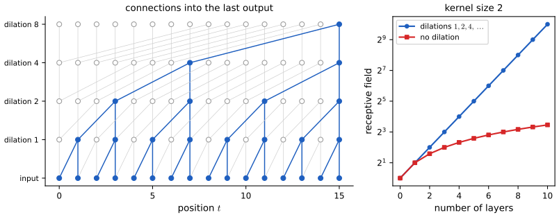
pp. 517–518 To generate, each output must depend only on previous outputs: a causal (or masked) convolution, giving a "convolutional Markov model" \[ p(\bm y)=\prod_{t=1}^Tp(y_t\given y_{1:t-1})=\prod_{t=1}^T\Cat\Big(y_t\,\Big|\,\softmax\Big(\varphi\Big(\sum_{\tau=1}^{t-k}\bm w^\T\bm y_{\tau:\tau+k}\Big)\Big)\Big), \tag{15.33} \] where \(\bm w\) is a filter of size \(k\) and one nonlinearity \(\varphi\) is assumed for notational simplicity. Dilated convolutions (Section 14.4.1) skip inputs to reach farther back at the same cost (Figure 15.15). WaveNet (van den Oord et al., 2016) stacks ten causal convolutional layers with dilations \(1,2,4,\dots,512\) into a block with receptive field 1024, left-padding every layer with zeros equal to its dilation so that all layers have the same length, and repeats this block three times; the conditioning \(\bm x\) is a set of linguistic features, and the output is raw audio. It sounds very natural but is slow to sample from; it can be distilled into a parallel model (van den Oord et al., 2018).
Filling the gap 15.12: the receptive field of a dilated causal stack, causality, and the factorisation (15.33) pp. 517–518, Figure 15.15
Derivation
Causal convolution. A layer with kernel size \(k\) and dilation \(d\) computes \(y_t=\sum_{j=0}^{k-1}\bm w_j\bm x_{t-jd}\) with \(\bm x_s=\bm 0\) for \(s\le0\), i.e. the input is padded on the left by \((k-1)d\) zeros (and not on the right). The output \(y_t\) then depends on \(x_s\) only for \(s\le t\), so the Jacobian \(\partial\bm y/\partial\bm x\) is lower triangular, and a stack of such layers is again lower triangular. A model whose \(t\)-th output is a function of \(y_{1:t-1}\) (shifted by one) defines the conditional \(p(y_t\given y_{1:t-1})\), and the product (15.33) is then a valid factorisation of a joint distribution by the chain rule, trained exactly by teacher forcing with all \(T\) conditionals computed in parallel. The numerical experiment verifies that changing the inputs after time 20 leaves all outputs before time 20 unchanged and that the construction equals a standard library convolution with left padding.
Receptive field. The receptive field of an output is the set of input positions that can affect it. Claim: for a stack of causal convolutions with kernel size \(k\) and dilations \(d_1,\dots,d_L\) it has size \[ R=1+(k-1)\sum_{l=1}^Ld_l . \] Proof. By induction on the number of layers. With one layer, \(y_t\) depends on \(x_t,x_{t-d_1},\dots,x_{t-(k-1)d_1}\), i.e. on a window of size \(1+(k-1)d_1\). Suppose the first \(l-1\) layers have receptive field a window \([t-(R_{l-1}-1),t]\) at the output position \(t\). Layer \(l\) reads outputs of layer \(l-1\) at \(t,t-d_l,\dots,t-(k-1)d_l\); the union of their windows is \([t-(k-1)d_l-(R_{l-1}-1),t]\) provided consecutive windows overlap or touch, i.e. \(d_l\le R_{l-1}\) (otherwise there are gaps, and the field is not contiguous). The size is \(R_{l-1}+(k-1)d_l\). \(\square\)
For WaveNet, \(k=2\) and \(d_l=2^{l-1}\), \(l=1,\dots,10\): \(R=1+\sum_{l=0}^92^l=1+1023=1024\), as the book states; three such blocks give \(R=1+3\cdot1023=3070\). With doubling dilations \(d_l=2^{l-1}\) one has \(d_l\le R_{l-1}=2^{l-1}\) with equality, so the field is a contiguous window (Figure 15.15, left: the last output depends on all 16 inputs with four layers). The number of layers needed to cover a window of \(n\) inputs is \(\lceil\log_kn\rceil\) with dilations \(k^{l-1}\) (receptive field \(k^L\), which is the \(\log_kn\) path length of Table 15.1), against \(\lceil(n-1)/(k-1)\rceil\) for undilated convolutions (Figure 15.15, right). The formula was confirmed by perturbing each input of random tanh networks and counting the inputs that move the last output: 64 for six layers of kernel 2 with dilations \(1,2,\dots,32\), and 81 for kernel 3 with dilations \(1,3,9,27\). \(\square\)
15.4 Attention
pp. 518–519 So far every hidden activation was a linear function of the inputs followed by a nonlinearity, \(\bm Z=\varphi(\bm X\bm W)\) with a fixed matrix \(\bm W\) learned on the training set. Attention makes the weights depend on the input, \(\bm Z=\varphi(\bm X\bm W(\bm X))\), through a multiplicative interaction: more generally \(\bm Z=\varphi(\bm V\bm W(\bm Q,\bm K))\) where the queries \(\bm Q\) say what each position is looking for, the keys \(\bm K\) say what each position contains, and the values \(\bm V\) say what it transmits; they are usually linear projections \(\bm Q=\bm W_q\bm X\), \(\bm K=\bm W_k\bm X\), \(\bm V=\bm W_v\bm X\) of the input. The output for query \(\bm q_j\) is \(\bm z_j=\sum_i\alpha_{ij}\bm v_i\) with weights \(0\le\alpha_{ij}\le1\), \(\sum_i\alpha_{ij}=1\) (Figure 15.16): the output is a data-dependent average of the inputs, and what is learned is the three projection matrices.
See also: Foundations of Deep Learning, Section 12.1 (attention); the attention explorer demonstration.
15.4.1 Attention as soft dictionary lookup
pp. 519–520 Fix one query \(\bm q\). A dictionary lookup compares \(\bm q\) to every key \(\bm k_i\) and returns the matching value; to make it differentiable one returns a convex combination, \[ \Attn\big(\bm q,(\bm k_1,\bm v_1),\dots,(\bm k_m,\bm v_m)\big)=\sum_{i=1}^m\alpha_i(\bm q,\bm k_{1:m})\bm v_i\in\R^v, \tag{15.34} \] \[ \alpha_i(\bm q,\bm k_{1:m})=\softmax_i\big([a(\bm q,\bm k_1),\dots,a(\bm q,\bm k_m)]\big)=\frac{\exp(a(\bm q,\bm k_i))}{\sum_{j=1}^m\exp(a(\bm q,\bm k_j))}, \tag{15.35} \] where \(a(\bm q,\bm k_i)\in\R\) is an attention score (a similarity). To restrict attention to valid entries (for example to ignore padding, or future positions as in causal convolution) one masks: the score of a forbidden entry is set to a large negative number such as \(-10^6\) so that its softmax weight is zero.
Filling the gap 15.13: properties of soft attention (convex combination, masking, permutation behaviour, the Jacobian) and soft versus hard attention pp. 519–520, 525–526, (15.34), (15.35)
Derivation
(a) Convex combination. The weights \(\alpha_i>0\) sum to one, so \(\bm z=\sum_i\alpha_i\bm v_i\) lies in the convex hull of the values; in particular \(\|\bm z\|\le\max_i\|\bm v_i\|\) (triangle inequality). If all keys are equal, all scores are equal and \(\bm z\) is the mean of the values.
(b) Masking. Softmax is invariant to adding a constant to all scores. Adding \(-10^6\) to the score of a masked entry multiplies its unnormalised weight by \(e^{-10^6}\), which is exactly 0 in double precision (the underflow threshold is \(e^{-745}\)) whenever the other scores are within a few hundred of each other; so the weights equal those obtained with a \(-\infty\) mask, as the numerical experiment confirms bit for bit. The constant \(-10^6\) has the advantage over \(-\infty\) that a query with all entries masked yields uniform weights instead of the undefined \(0/0\).
(c) Permutations. Permuting the (key, value) pairs jointly permutes the terms of the sum and the entries of the softmax, so (15.34) is invariant to the order of the pairs. Permuting the queries permutes the outputs: \(\Attn(\bm Q\bm\Pi,\cdot)=\bm\Pi\,\Attn(\bm Q,\cdot)\). So self-attention without positional information (Section 15.5.1) is permutation equivariant: \(\operatorname{SA}(\bm\Pi\bm X)=\bm\Pi\operatorname{SA}(\bm X)\), not invariant as the book says in Section 15.5.3 (the output is permuted, not unchanged; invariance follows only after an order-insensitive pooling). Adding a positional code breaks the symmetry, as intended.
(d) The Jacobian of the weights. With \(\bm s\) the vector of scores, \(\partial\bm\alpha/\partial\bm s=\diag(\bm\alpha)-\bm\alpha\bm\alpha^\T\), a positive semi-definite matrix (it is the covariance matrix of the one-hot vector drawn with probabilities \(\bm\alpha\)) with eigenvalues in \([0,\frac12]\). When \(\bm\alpha\) is close to a vertex of the simplex every entry \(\alpha_i(\delta_{ij}-\alpha_j)\) is small, so the Jacobian vanishes: a saturated softmax passes no gradient to the scores. This is why the scale of the scores matters (gap 15.15).
(e) Soft against hard attention (Section 15.4.7). Hard attention samples one index \(I\sim\alpha\) and uses \(\bm v_I\); soft attention uses the mean \(\E_{I\sim\alpha}[\bm v_I]=\sum_i\alpha_i\bm v_i\). The soft output is a differentiable function of the scores, so ordinary backpropagation applies. The hard objective \(\E_{I\sim\alpha_\theta}[L(\bm v_I)]=\sum_i\alpha_{\theta,i}L(\bm v_i)\) is differentiable in \(\theta\) only through the probabilities, and its gradient, \(\sum_i L(\bm v_i)\nabla_\theta\alpha_{\theta,i}=\E_{I}[L(\bm v_I)\nabla_\theta\log\alpha_{\theta,I}]\) (the log-derivative identity \(\nabla\alpha=\alpha\nabla\log\alpha\)), has to be estimated by sampling (REINFORCE), with high variance and the need for a baseline; this is why the book says hard attention requires reinforcement learning. For a convex loss, Jensen's inequality gives \(L(\E[\bm v_I])\le\E[L(\bm v_I)]\): the soft model's loss is a lower bound of the hard model's expected loss. \(\square\)
15.4.2 Kernel regression as non-parametric attention
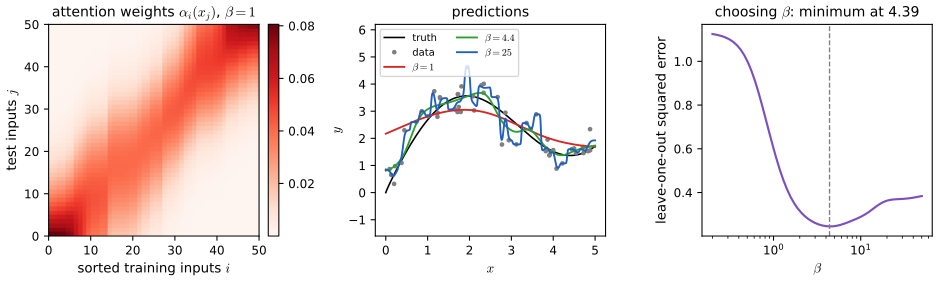
pp. 520–521 Kernel regression (Section 16.3.5) predicts at a query point \(x\) a weighted combination of all training labels, \(f(x)=\sum_{i=1}^n\alpha_i(x,x_{1:n})y_i\) (15.36), with weights proportional to a similarity: with the Gaussian density kernel \(K_\sigma(u)=(2\pi\sigma^2)^{-1/2}e^{-u^2/(2\sigma^2)}\) (15.37) one sets \(a(x,x_i)=K_\sigma(x-x_i)\); the constant cancels on normalisation, and writing \(\beta^2=1/\sigma^2\) (so \(K(u;\beta)=\exp(-\beta^2u^2/2)\), 15.38), \[ f(x)=\sum_{i=1}^n\frac{\exp[-\frac12((x-x_i)\beta)^2]}{\sum_{j=1}^n\exp[-\frac12((x-x_j)\beta)^2]}\,y_i=\sum_{i=1}^n\softmax_i\big(-\tfrac12\beta^2(x-x_1)^2,\dots,-\tfrac12\beta^2(x-x_n)^2\big)y_i . \tag{15.39–15.41} \] This is attention with the test points as queries, the training inputs as keys and the training labels as values (Figure 15.17). Increasing \(\beta\) (shrinking the bandwidth) narrows the diagonal band of the attention matrix and eventually overfits. My version of Figure 15.17 uses \(n=50\) sorted inputs on \([0,5]\) from \(y=2\sin x+x^{0.8}+\varepsilon\), \(\varepsilon\sim\N(0,0.5^2)\), a stand-in for the book's data.
Filling the gap 15.14: the Nadaraya–Watson estimator derived three ways, and the limits \(\beta\to0\) and \(\beta\to\infty\) pp. 520–521, (15.36)–(15.41)
Derivation
Let \(K\ge0\) be a symmetric kernel and \(w_i(x)=K(x-x_i)\). (i) Locally constant least squares. Choose the constant \(m\) that best fits the labels near \(x\): minimise \(\sum_iw_i(x)(y_i-m)^2\). Setting the derivative to zero, \(-2\sum_iw_i(y_i-m)=0\), gives \(m=\sum_iw_iy_i/\sum_iw_i\), (15.36) with \(\alpha_i=w_i/\sum_jw_j\); the objective is a convex quadratic, so this is the unique minimiser. (ii) Conditional mean of a kernel density. Estimate the joint density by \(\hat f(x,y)=\frac1n\sum_iK_h(x-x_i)K_{h'}(y-y_i)\) with a symmetric \(K_{h'}\) of mean zero. Then \(\int y\,\hat f(x,y)\,\mathrm dy=\frac1n\sum_iK_h(x-x_i)\,y_i\) (because \(\int yK_{h'}(y-y_i)\,\mathrm dy=y_i\)) and \(\hat f(x)=\int\hat f(x,y)\,\mathrm dy=\frac1n\sum_iK_h(x-x_i)\), so \(\E[y\given x]=\hat f(x)^{-1}\int y\hat f(x,y)\,\mathrm dy\) is again the weighted average. (iii) Attention form. With \(K(u)=\exp(-\beta^2u^2/2)\), \(\alpha_i=\exp(s_i)/\sum_j\exp(s_j)\) with \(s_i=-\frac12\beta^2(x-x_i)^2\), i.e. (15.41): the normalising constant \(1/\sqrt{2\pi\sigma^2}\) of the Gaussian cancels, as the book says. The numerical experiment confirms that (15.41), the explicit ratio and the minimiser of the weighted least-squares problem (found by a one-dimensional optimiser) coincide to \(10^{-10}\).
Limits. As \(\beta\to0\), \(s_i\to0\) for every \(i\) and \(\alpha_i\to1/n\): \(f(x)\to\bar y\), the global mean (maximal smoothing, high bias). As \(\beta\to\infty\), \(s_i-s_{i^\star}=-\frac12\beta^2[(x-x_i)^2-(x-x_{i^\star})^2]\to-\infty\) for the nearest training input \(i^\star\) (assumed unique), so \(\alpha_{i^\star}\to1\) and \(f(x)\to y_{i^\star}\): nearest-neighbour regression, which interpolates the training data (zero training error at distinct inputs) and has high variance. Between the two, the bandwidth \(1/\beta\) trades bias against variance, and the leave-one-out score \(\frac1n\sum_i(y_i-\hat f_{-i}(x_i))^2\), with \(\hat f_{-i}\) computed by deleting the diagonal weight (the softmax over the other \(n-1\) points), selects it (Figure 15.17, right; agrees with brute-force deletion to \(10^{-12}\)). Computing the prediction at one query costs \(O(n)\) and all test points \(O(mn)\): the model keeps the whole training set, which is why the book turns to parametric attention next. \(\square\)
See also: Nonparametric Statistical Inference, Definition 5.39 (Nadaraya–Watson), Section 5.3 (choosing the smoothing parameter); Elements of Statistical Learning, Section 6.1.
15.4.3 Parametric attention
p. 521 Non-parametric methods scale badly in the number of training points and the dimension, so one fixes the keys and values and compares queries and keys in a learned embedding space. If \(\bm q\in\R^q\) and \(\bm k\in\R^k\) have different sizes, map both to \(\R^h\) and use an MLP: the additive attention score \[ a(\bm q,\bm k)=\bm w_v^\T\tanh(\bm W_q\bm q+\bm W_k\bm k)\in\R. \tag{15.42} \] More efficient is to give queries and keys the same length \(d\) and use \(\bm q^\T\bm k\); if the entries are independent with mean 0 and variance 1 then \(\E[\bm q^\T\bm k]=0\) and \(\var[\bm q^\T\bm k]=d\), so one divides by \(\sqrt d\) to keep the variance at 1 for any \(d\): scaled dot-product attention \[ a(\bm q,\bm k)=\bm q^\T\bm k/\sqrt d\in\R, \tag{15.43} \] and for minibatches of queries \(\bm Q\in\R^{n\times d}\), keys \(\bm K\in\R^{m\times d}\) and values \(\bm V\in\R^{m\times v}\), \[ \Attn(\bm Q,\bm K,\bm V)=\softmax\Big(\frac{\bm Q\bm K^\T}{\sqrt d}\Big)\bm V\in\R^{n\times v}, \tag{15.44} \] with the softmax taken row-wise.
Filling the gap 15.15: why \(\sqrt d\): the variance of \(\bm q^\T\bm k\), and what happens to the softmax without the scaling p. 521, (15.43), (15.44)
Derivation
Variance. Let \(q_1,\dots,q_d,k_1,\dots,k_d\) be independent with \(\E q_i=\E k_i=0\) and \(\var q_i=\var k_i=1\). Then \(\E[q_ik_i]=\E q_i\E k_i=0\), and since the products \(q_ik_i\) are independent over \(i\) (they involve disjoint coordinates), \(\E[\bm q^\T\bm k]=0\) and \[ \var[\bm q^\T\bm k]=\sum_{i=1}^d\var[q_ik_i]=\sum_{i=1}^d\E[q_i^2]\E[k_i^2]=d \] (\(\var[q_ik_i]=\E[q_i^2k_i^2]-(\E[q_ik_i])^2=\E[q_i^2]\E[k_i^2]\) by independence). This is the book's pair of results (2.34) and (2.39), and it needs only independence, mean zero and unit variance, not Gaussianity (verified for Gaussian and for uniform entries, \(d=64\), within 2 percent). Dividing by \(\sqrt d\) divides the variance by \(d\) and gives 1.
Why it matters. The scores that enter the softmax have standard deviation \(\sqrt d\) when unscaled. For \(m\) keys the largest of \(m\) independent \(\N(0,d)\) scores exceeds the typical one by about \(\sqrt{2d\ln m}\), so when \(d\) is large one score dominates and the weights \(\alpha\) are almost one-hot: the entropy of the attention drops towards 0, the output is a single value, and by gap 15.13(d) the Jacobian \(\diag(\bm\alpha)-\bm\alpha\bm\alpha^\T\) is close to zero, so the gradient with respect to the scores, and hence to \(\bm W_q,\bm W_k\), vanishes. With the scaling the scores are \(O(1)\) whatever \(d\) is, so initial attention is diffuse and trainable. (The demonstration Positional encoding and attention scores simulates this: for \(d=256\) and 10 keys the unscaled attention puts almost all its mass on one key, the scaled one does not.) The additive score (15.42) is bounded by \(\|\bm w_v\|_1\) and needs no such correction. \(\square\)
15.4.4 Seq2Seq with attention
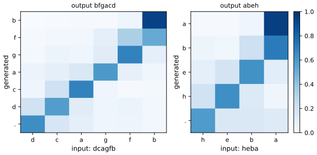
pp. 522–523 In the encoder-decoder of Section 15.2.3.2 the decoder state is \(\bm h^d_t=f_d(\bm h^d_{t-1},y_{t-1},\bm c)\) with a fixed-length context \(\bm c=\bm h^e_T\): the output cannot look at the input words themselves, and word order differs between languages, so the alignment between source and target must be inferred. The remedy (Bahdanau et al., 2015; Luong et al., 2015) replaces \(\bm c\) by a dynamic context computed by attention, \[ \bm c_t=\sum_{i=1}^T\alpha_i(\bm h^d_{t-1},\bm h^e_{1:T})\,\bm h^e_i, \tag{15.45} \] with the previous decoder state as the query and the encoder states as keys and values; \(\bm c_t\) is concatenated with \(y_{t-1}\) and fed with \(\bm h^d_{t-1}\) to produce \(\bm h^d_t\) (Figure 15.18). The attention weights, plotted as a heat map, show which input the model used for each output (Figure 15.19).
My version trains the encoder-decoder on a task with a known alignment: reversing a string of 3 to 8 letters (GRU encoder and decoder, 64 units, scaled dot-product attention, teacher forcing, 1200 steps). It stands in for the book's Spanish-to-English translation, which needs data and compute outside the scope of a CPU. The heat map is the anti-diagonal one expects.
15.4.5 Seq2vec with attention
p. 523 Attention also helps classifiers. Rajkomar et al. (2018) apply an RNN to electronic health records (structured data and clinical notes) to predict whether a patient will die; attention picks out the relevant parts of the input (Figure 15.20, an example from the paper that is not reproduced). In seq2vec form, the classifier reads \(\bm z=\sum_i\alpha_i\bm h_i\) with a learned query vector instead of the last state or a plain average.
15.4.6 Seq+Seq2Vec with attention
pp. 523–525 In textual entailment (natural language inference) a premise \(A=(\bm a_1,\dots,\bm a_m)\) and a hypothesis \(B=(\bm b_1,\dots,\bm b_n)\), with word embeddings \(\bm a_i,\bm b_j\in\R^E\), are classified into entailment, contradiction or neutral (a standard benchmark is the SNLI corpus of 550,000 labelled pairs). The decomposable attention model of Parikh et al. (2016) has three steps. First, each \(\bm a_i\) attends to the words of \(B\): \(e_{ij}=f(\bm a_i)^\T f(\bm b_j)\) with an MLP \(f:\R^E\to\R^D\) (15.46), and \(\bm\beta_i=\sum_{j=1}^n\frac{\exp(e_{ij})}{\sum_{k=1}^n\exp(e_{ik})}\bm b_j\) (15.47) is the part of the hypothesis that aligns with \(\bm a_i\). Second, compare: \(\bm v_{A,i}=g([\bm a_i,\bm\beta_i])\) with an MLP \(g:\R^{2E}\to\R^H\) (15.48). Third, aggregate: \(\bm v_A=\sum_{i=1}^m\bm v_{A,i}\) (15.49), and symmetrically \(\bm\alpha_j=\sum_{i=1}^m\frac{\exp(e_{ij})}{\sum_{k=1}^m\exp(e_{kj})}\bm a_i\) (15.50), \(\bm v_{B,j}=g([\bm b_j,\bm\alpha_j])\) (15.51), \(\bm v_B=\sum_{j=1}^n\bm v_{B,j}\) (15.52). A final MLP \(h:\R^{2H}\to\R^3\) gives \(\hat y=h([\bm v_A,\bm v_B])\) (15.53). The pairwise scores \(e_{ij}\) cost \(O(mn)\), and because the aggregation is a sum, the prediction does not depend on the order of the words within a sentence, except through the embeddings. Changing the output layer gives other pair tasks, for instance semantic textual similarity (scores from 0 to 5 on the STS benchmark).
15.4.7 Soft vs hard attention
pp. 525–526 If the heat map is forced to be sparse, so that each output attends to a single input, the method is hard attention; the training objective is then not differentiable and one uses reinforcement-learning estimators (Xu et al., 2015; the captioning example of Figure 15.22 is a figure from that paper and is not reproduced). The relation between the two and the reason hard attention needs a score-function estimator are derived in gap 15.13(e). Attention heat maps look like explanations of the model's output, but their interpretability is controversial (Jain and Wallace, 2019; Wiegreffe and Pinter, 2019; Serrano and Smith, 2019; Brunner et al., 2019): the weights describe where the information was read from in one layer, not which inputs caused the output.
15.5 Transformers
p. 526 The transformer (Vaswani et al., 2017) is a seq2seq model that uses attention in the encoder as well as in the decoder, so that no recurrence is needed. It has been used for machine translation, parsing, music, protein sequences, summarisation and, treating an image as a raster-scanned sequence, image generation. It is assembled from several new blocks, introduced below.
See also: Foundations of Deep Learning, Section 12.1.7 (transformer layers), 12.3.1 (decoder transformers) and the character-level transformer demonstration.
15.5.1 Self-attention
pp. 526–527 In Section 15.4.4 the decoder attended to the encoder. If instead a sequence attends to itself one gets self-attention: for inputs \(\bm x_1,\dots,\bm x_n\in\R^d\) the outputs of the same size are \[ \bm y_i=\Attn\big(\bm x_i,(\bm x_1,\bm x_1),\dots,(\bm x_n,\bm x_n)\big), \tag{15.54} \] with query \(\bm x_i\) and keys and values all the (valid) inputs (in practice after the projections \(\bm W_q,\bm W_k,\bm W_v\)). In a decoder one sets \(\bm x_i=\bm y_{i-1}\) and restricts the keys to \(\bm x_{1:i}\) (all previously generated outputs); at training time all outputs are known, so the \(n\) outputs can be computed in parallel, which removes the sequential bottleneck of an RNN. Self-attention also gives contextual representations: in "the animal didn't cross the street because it was too tired" the representation of "it" attends to "animal", and to "street" when the sentence ends "too wide" (Figure 15.23, a visualisation from the Google AI blog that is not reproduced), which is the coreference resolution needed to choose the gender of a French pronoun.
15.5.2 Multi-headed attention
pp. 527–528 An attention matrix behaves like a kernel matrix (Section 15.4.2), and one may want several, capturing different notions of similarity. Given \(\bm q\in\R^{d_q}\), \(\bm k_j\in\R^{d_k}\), \(\bm v_j\in\R^{d_v}\), head \(i\) is \[ \bm h_i=\Attn\big(\bm W_i^{(q)}\bm q,\{\bm W^{(k)}_i\bm k_j,\bm W_i^{(v)}\bm v_j\}\big)\in\R^{p_v}, \tag{15.55} \] with \(\bm W_i^{(q)}\in\R^{p_q\times d_q}\), \(\bm W_i^{(k)}\in\R^{p_k\times d_k}\), \(\bm W_i^{(v)}\in\R^{p_v\times d_v}\), and the \(h\) heads are stacked and projected: \[ \bm h=\MHA(\bm q,\{\bm k_j,\bm v_j\})=\bm W_o\begin{pmatrix}\bm h_1\\\vdots\\\bm h_h\end{pmatrix}\in\R^{p_o},\qquad\bm W_o\in\R^{p_o\times hp_v}. \tag{15.56} \] If \(p_qh=p_kh=p_vh=p_o\) all heads can be computed in parallel (Figure 15.24).
Filling the gap 15.16: multi-head attention as a sum of rank-limited heads, and its cost pp. 527–528, (15.55), (15.56)
Derivation
Concatenate-then-project equals sum-of-projections. Split \(\bm W_o=[\bm W_o^{(1)}\ \cdots\ \bm W_o^{(h)}]\) into blocks of \(p_v\) columns. Then \(\bm W_o[\bm h_1;\dots;\bm h_h]=\sum_{i=1}^h\bm W_o^{(i)}\bm h_i\). For a sequence of queries stacked in the rows of \(\bm X\) (self-attention, row-vector convention), \(\bm h_i=\bm A^{(i)}\bm X\bm W_v^{(i)}\) with \(\bm A^{(i)}=\softmax(\bm X\bm W_q^{(i)}\bm W_k^{(i)\T}\bm X^\T/\sqrt{p})\), so the whole layer is \[ \MHA(\bm X)=\sum_{i=1}^h\bm A^{(i)}\,\bm X\,\bm B^{(i)},\qquad\bm B^{(i)}=\bm W_v^{(i)}\bm W_o^{(i)\T}, \] a sum of \(h\) terms, each mixing positions with its own attention matrix \(\bm A^{(i)}\) and transforming features with a matrix \(\bm B^{(i)}\) of rank at most \(p_v\). The score matrix of head \(i\), \(\bm W_q^{(i)}\bm W_k^{(i)\T}\), also has rank at most \(p\); one head with full width \(d\) could express any bilinear score, but only one attention pattern.
Cost. With \(d_q=d_k=d_v=p_o=d\) and \(p_q=p_k=p_v=d/h\), the projections of all heads together have \(3d^2\) weights, \(\bm W_o\) has \(d^2\), so the layer has \(4d^2\) parameters, the same as a single head of width \(d\); computing the scores of all heads costs \(h\cdot n^2\cdot(d/h)=n^2d\) multiply-adds, again the same. Multi-head attention does not add parameters or asymptotic cost, it spends the same budget on \(h\) different, lower-rank attention patterns. The code's implementation agrees with a standard library layer (outputs and per-head weights) to \(10^{-10}\) when the weights are copied across. \(\square\)
15.5.3 Positional encoding
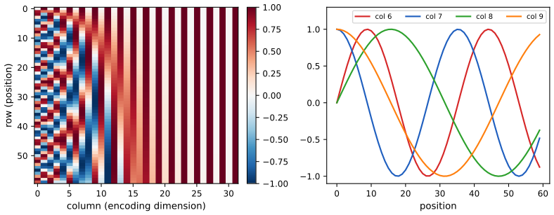
pp. 528–529 Self-attention ignores the order of the inputs (gap 15.13(c)), so a positional encoding is added to the word embeddings. A first idea is to write the integer position in binary, one bit per dimension; for \(n=8\) the 3-bit codes are \(000,001,\dots,111\), the right-most bit toggles fastest and the left-most slowest. This is a set of basis functions (powers of 2) with 0/1 coefficients. A more compact, real-valued code uses sinusoids (Vaswani et al., 2017), \[ p_{i,2j}=\sin\Big(\frac{i}{C^{2j/d}}\Big),\qquad p_{i,2j+1}=\cos\Big(\frac{i}{C^{2j/d}}\Big),\qquad C=10{,}000, \tag{15.57} \] so for \(d=4\), \(\bm p_i=[\sin(i/C^{0}),\cos(i/C^0),\sin(i/C^{1/2}),\cos(i/C^{1/2})]\) (15.58). Figure 15.25a shows the matrix \(\bm P\in\R^{n\times d}\) for \(n=60\), \(d=32\): each row is a real-valued fingerprint of its position and the left-most columns oscillate fastest; panel (b) shows columns 6 to 9. Two advantages: it can be computed for any length up to about \(C\), unlike a learned map from integers; and the code of one position is a linear function of the code of another at a known offset \(\phi\), \(\bm p_{t+\phi}=f(\bm p_t)\), because \[ \begin{pmatrix}\sin(\omega_k(t+\phi))\\\cos(\omega_k(t+\phi))\end{pmatrix}=\begin{pmatrix}\cos(\omega_k\phi)&\sin(\omega_k\phi)\\-\sin(\omega_k\phi)&\cos(\omega_k\phi)\end{pmatrix}\begin{pmatrix}\sin(\omega_kt)\\\cos(\omega_kt)\end{pmatrix},\qquad\omega_k=C^{-2k/d}, \tag{15.59, 15.60} \] and the code is combined with the embeddings \(\bm X\) by addition, \(\operatorname{POS}(\operatorname{Embed}(\bm X))=\bm X+\bm P\) (15.61). The book adds that "if \(\phi\) is small then \(\bm p_{t+\phi}\approx\bm p_t\)", a useful inductive bias.
Filling the gap 15.17: the rotation property, a similarity that depends only on the offset, and when \(\bm p_{t+\phi}\approx\bm p_t\) is true pp. 528–529, (15.57)–(15.61)
Derivation
Write \(\omega_k=C^{-2k/d}\), \(k=0,\dots,d/2-1\), and \(\bm p_t=(\sin\omega_0t,\cos\omega_0t,\dots,\sin\omega_{d/2-1}t,\cos\omega_{d/2-1}t)\).
Rotation (15.59), (15.60). The addition formulas \(\sin(a+b)=\sin a\cos b+\cos a\sin b\) and \(\cos(a+b)=\cos a\cos b-\sin a\sin b\) with \(a=\omega_kt\), \(b=\omega_k\phi\) give the matrix identity displayed above. The matrix \(\bm R_k(\phi)\) is a rotation by angle \(-\omega_k\phi\) (determinant 1, orthogonal) that depends on the offset \(\phi\) but not on \(t\); the book's second row has typos (it omits the index \(k\) in one \(\omega\)). Stacking the \(d/2\) blocks, \(\bm p_{t+\phi}=\bm R(\phi)\bm p_t\) with \(\bm R(\phi)=\operatorname{blockdiag}(\bm R_0(\phi),\dots,\bm R_{d/2-1}(\phi))\) orthogonal. So a position shift is the same linear map wherever you are in the sequence, which is what lets attention learn "look \(\phi\) steps back" with a fixed bilinear form.
Similarity and norm. Each block has \(\sin^2+\cos^2=1\), so \(\|\bm p_t\|^2=d/2\) for every \(t\). The inner product of two codes is \[ \bm p_t^\T\bm p_{t+\phi}=\sum_{k}\big[\sin\omega_kt\sin\omega_k(t+\phi)+\cos\omega_kt\cos\omega_k(t+\phi)\big]=\sum_k\cos(\omega_k\phi), \] independent of \(t\) (Figure 15.S6, left and middle): the position-position part of an attention score depends on the relative offset only, decays as \(\phi\) grows and has the shape of a sum of cosines with geometrically spaced frequencies.
When is \(\bm p_{t+\phi}\approx\bm p_t\)? Using \(\|\bm R_k(\phi)\bm u-\bm u\|=2|\sin(\omega_k\phi/2)|\,\|\bm u\|\) for the unit vector \(\bm u\) of block \(k\), \[ \|\bm p_{t+\phi}-\bm p_t\|^2=4\sum_{k=0}^{d/2-1}\sin^2\Big(\frac{\omega_k\phi}{2}\Big)\le\phi^2\sum_k\omega_k^2 . \] For the first block \(\omega_0=1\), so already a shift of one position changes it by \(2\sin(\tfrac12)=0.96\): the claim holds only for the slow dimensions. For \(d=32\) the full vector changes by 1.17 per step (against a norm of 4, about 29 percent), almost all of it in the fastest few pairs, while the 16 slowest coordinates change by 0.012 (Figure 15.S6, right). So position codes of nearby positions are similar, but not close in norm.
Adding versus concatenating. (15.61) uses \(\bm x_i+\bm p_i\). In a first-layer score the cross terms appear: \((\bm x_i+\bm p_i)^\T\bm W_q^\T\bm W_k(\bm x_j+\bm p_j)\) expands into content–content, content–position, position–content and position–position terms. This is also what a concatenation \([\bm x;\bm p]\) with a block weight matrix would give, so adding loses nothing as long as the embedding can be learned to avoid the coordinates used by \(\bm p\) (the book's footnote 5), and it saves the extra dimensions. The wavelengths \(2\pi C^{2k/d}\) form a geometric progression from \(2\pi\) to about \(2\pi C\), the continuous analogue of the binary code in which bit \(j\) toggles every \(2^j\) positions. \(\square\)
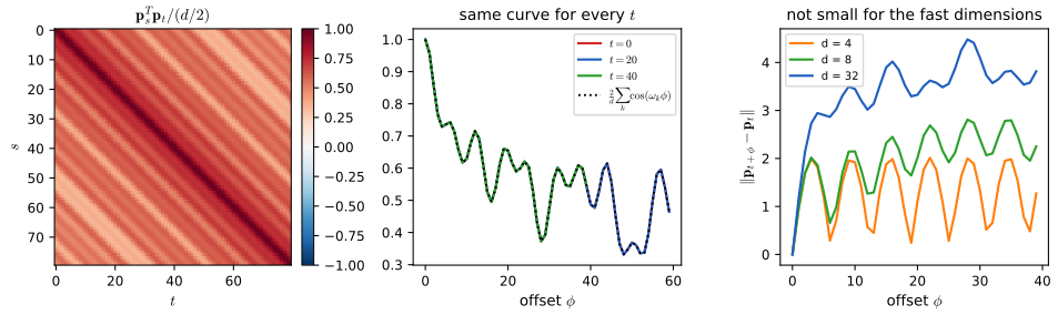
15.5.4 Putting it all together
pp. 529–531 The transformer is a seq2seq model whose encoder and decoder are stacks of blocks built from multi-head attention (15.5.2), residual connections (Section 13.4.4), feed-forward layers (13.2) and layer normalisation (14.2.4.2). The encoder block is
Z = LayerNorm(MultiHeadAttn(Q=X, K=X, V=X) + X),
E = LayerNorm(FeedForward(Z) + Z), and the encoder is
E = POS(Embed(X)) followed by \(N\) repetitions of the block (left of Figure 15.26). The decoder block additionally attends to the encoder output \(\bm E\) with a second multi-head block (keys and values \(\bm E\)), after a first masked (causal) self-attention over the previously generated outputs (shifted right and given positional codes):
Z = LayerNorm(MultiHeadAttn(Q=Y, K=Y, V=Y) + Y), Z' = LayerNorm(MultiHeadAttn(Q=Z, K=E, V=E) + Z), D = LayerNorm(FeedForward(Z') + Z'); the distribution over tokens at every position is computed in parallel (right of Figure 15.26). At training time all decoder inputs \(\bm Y\) are known (lagged targets); at test time decoding is sequential and the generated output is appended to the keys and values that can be attended to, starting from a start-of-sequence token.
Filling the gap 15.18: causal masking gives parallel training and incremental decoding the same function; the cost table and the path lengths pp. 529–531, Table 15.1
Derivation
Masking and parallel decoding. Let \(\bm M\) be the lower-triangular mask (\(M_{ts}=1\) iff \(s\le t\)) and let the decoder use masked attention \(\softmax(\bm Q\bm K^\T/\sqrt d+\log\bm M)\bm V\). Row \(t\) of the weights vanishes for \(s>t\) (gap 15.13(b)), so the output at position \(t\) is a function of the inputs at positions \(\le t\) only. Every other operation of a block (residual connection, layer normalisation, feed-forward layer) is applied to each position separately, so by induction over the layers the representation at position \(t\) after any number of blocks depends only on the inputs \(\bm y_{1:t}\) and equals what the same network computes when it is run on the prefix \(\bm y_{1:t}\) alone, with \(t\) as the last position. Running the network once on the whole sequence therefore gives the \(n\) next-token predictions that \(n\) separate incremental runs (with a cache of the keys and values of all earlier positions at every layer) would give. The numerical experiment on a two-layer decoder confirms equality to \(10^{-12}\). So training with teacher forcing is a single parallel pass that is mathematically identical to sequential decoding, which is the benefit stated at the start of the section; inference is still sequential because the inputs at position \(t+1\) are the samples drawn at \(t\), but the cache avoids recomputing the earlier positions.
Cost per layer (Table 15.1). Take \(n\) positions and \(d\) features. Self-attention: the score matrix \(\bm Q\bm K^\T\) costs \(n^2d\) multiply-adds and the weighted sum \(\bm A\bm V\) another \(n^2d\), i.e. \(O(n^2d)\) (the four projections add \(4nd^2\), which is lower order when \(n>d\)); all positions are computed in parallel, so there are \(O(1)\) sequential operations, and every output depends directly on every input: maximum path length \(O(1)\). Recurrent: each step multiplies the \(d\times d\) matrices \(\bm W_{hh},\bm W_{xh}\) by a vector, \(O(d^2)\), for \(n\) steps: \(O(nd^2)\), with \(n\) sequential operations, and the path from \(x_1\) to \(h_n\) has \(n\) steps. Convolutional (kernel \(k\), \(d\) channels in and out): \(kd^2\) per position, \(O(knd^2)\) in parallel; to connect two positions \(n\) apart one needs a receptive field \(n\), \(\lceil(n-1)/(k-1)\rceil\) undilated layers or \(\lceil\log_kn\rceil\) layers with dilations \(k^{l}\) (gap 15.12). The attention layer is cheaper than the recurrent one iff \(2n^2d<2nd^2\), i.e. \(n<d\), the condition the book states loosely as \(n\ll d\). The counts of my implementation (2 per attention head \(\times n^2d\)) equal the formula, and the path lengths measured on the dependency graph of the recurrent network and from the formulas agree (Figure 15.S3).
Parameters of one block. Multi-head attention \(4d^2\) (+ biases), a feed-forward layer of width \(d_{\rm ff}\) with \(2dd_{\rm ff}\) (+ biases), and layer normalisation \(2d\) per norm. For the usual \(d_{\rm ff}=4d\) this is about \(12d^2\), two thirds of it in the feed-forward layers. \(\square\)
15.5.5 Comparing transformers, CNNs and RNNs
pp. 531–532 Figure 15.27 compares a 1d CNN, an RNN and an attention model mapping \(\bm x_{1:n}\) to \(\bm y_{1:n}\); the trade-offs are summarised by the maximum path length between any two inputs (how many steps a signal or a gradient needs to travel) and the cost of one layer.
| Layer type | Complexity per layer | Sequential operations | Maximum path length |
|---|---|---|---|
| Self-attention | \(O(n^2d)\) | \(O(1)\) | \(O(1)\) |
| Recurrent | \(O(nd^2)\) | \(O(n)\) | \(O(n)\) |
| Convolutional | \(O(knd^2)\) | \(O(1)\) | \(O(\log_kn)\) (dilated) |
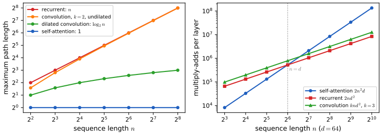
15.5.6 Transformers for images *
pp. 532–533 CNNs have useful inductive biases for images: locality (small kernels), equivariance (weight tying) and invariance (pooling). It is nevertheless possible to classify images with a transformer, provided there is enough data to make up for the missing bias (Raghu et al., 2021). The vision transformer (ViT; Dosovitskiy et al., 2021) cuts the image into \(16\times16\) patches, projects each patch to an embedding, prepends a learnable [CLASS] embedding \(\bm x_0\), adds positional embeddings and sends the sequence \(\bm x_{0:T}\) to a transformer encoder; the output \(\bm e_0\) at position 0 is mapped to the class label (Figure 15.28). After pretraining and fine-tuning (transfer learning, Section 19.2) ViT is better than the ResNet BiT on large pretraining sets (ImageNet-21k, JFT-300M) but not on ImageNet alone, and it is cheaper to train than a ResNet at that scale, although the large model still takes 30 days on 8 TPU cores. (Later work showed that a modernised CNN, ConvNeXt, can match ViT.)
Filling the gap 15.19: patch embedding is a strided convolution, and what the patch size does to the sequence length pp. 532–533, Figure 15.28
Derivation
Let an image have \(C\) channels and size \(H\times W\), cut into non-overlapping \(p\times p\) patches. Flatten patch \((a,b)\) into a vector \(\bm u_{ab}\in\R^{p^2C}\) and project, \(\bm x_{ab}=\bm W_p^\T\bm u_{ab}\) with \(\bm W_p\in\R^{p^2C\times d}\). Entry \(c\) of the result is \(\sum_{i,j,\ell}W_p[(i,j,\ell),c]\,\text{image}[ap+i,\,bp+j,\,\ell]\): the correlation of the image with the \(c\)-th \(p\times p\times C\) filter evaluated at positions that are multiples of \(p\). That is exactly a convolutional layer with \(d\) output channels, kernel size \(p\) and stride \(p\) (no padding): patch embedding is a convolution, with weight tensor the reshaped \(\bm W_p\) (verified numerically against a library convolution). The sequence has \((H/p)(W/p)\) patch tokens plus the class token: \(14\cdot14+1=197\) for a \(224\times224\) image and \(p=16\). Attention over pixels as tokens would need \(224^2=50{,}176\) tokens and \(50{,}176^2\approx2.5\times10^9\) attention weights per head; patches reduce this by a factor \(p^4=65{,}536\), at the price of treating each patch as a single token. The class-token design makes the image-level prediction a function of one position that has attended to all others. Because the embedding has stride \(p\), the network is equivariant to translations that are multiples of \(p\) only; it is not translation equivariant at pixel level, one reason it needs more data than a CNN. \(\square\)
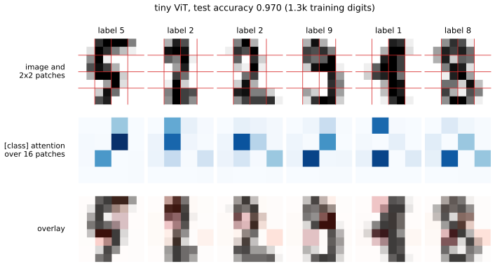
15.5.7 Other transformer variants *
p. 533 GShard (Lepikhin et al., 2021) scales transformers to many more parameters by replacing some feed-forward layers by a mixture of experts (Section 13.6.2): a gating network selects a few experts per token, giving sparse conditional computation, in which only part of the capacity is used for any input. The conformer (Gulati et al., 2020) inserts convolutional layers into the transformer block, which helps speech recognition.
15.6 Efficient transformers *
pp. 533–537 (This section of the book was written by Krzysztof Choromanski.) A regular transformer needs \(O(N^2)\) time and memory for a sequence of length \(N\), which is impractical for long sequences, and many variants reduce this (Figure 15.29 is a taxonomy diagram from Tay et al., 2020, not reproduced). The mathematics worth filling in is in Section 15.6.4; the first three families are summarised.
15.6.1 Fixed non-learnable localized attention patterns
p. 534 Restrict each token to attend to a preselected set of others. Chunking the sequence into \(K\) blocks of length \(N/K\) and attending only inside a block reduces the cost from \(O(N^2)\) to \(O(N^2/K)\) (Qiu et al., 2019; Parmar et al., 2018); strided or dilated windows and hybrids of several fixed patterns are also used (Child et al., 2019; Beltagy et al., 2020).
15.6.2 Learnable sparse attention patterns
p. 535 The partition into blocks can be learned: the attention is still restricted to the tokens within one part of a partition, but the partition is trained. With hashing (the Reformer, Kitaev et al., 2020) the parts are locality-sensitive-hashing buckets, requiring queries and keys to coincide, with time \(O(NM^2\log M)\) for embedding dimension \(M\); with clustering (Roy et al., 2020) tokens are clustered by \(K\)-means (Section 21.3), and with \(K=\Theta(\sqrt N)\) equal-size clusters the cost is \(O(N^{3/2})\), although equal sizes are hard to enforce.
15.6.3 Memory and recurrence methods
p. 535 A side memory module can read several tokens at once (global memory, as in Set Transformer and BigBird), or local blocks can be connected by recurrence (Transformer-XL, Dai et al., 2019).
15.6.4 Low-rank and kernel methods
pp. 535–537 Approximate the attention matrix by a low-rank factorisation, \[ A_{ij}=\bm\phi(\bm q_i)^\T\bm\phi(\bm k_j),\qquad\bm\phi(\bm x)\in\R^M, \tag{15.62} \] (Shen et al., 2018; Katharopoulos et al., 2020), after which \(\bm A\bm V\) can be computed in \(O(N)\) time by associativity. For softmax attention \(\bm A\) is not low rank, so one approximates it: Linformer (Wang et al., 2020) projects keys and values with random Gaussian matrices and uses the Johnson–Lindenstrauss transform; the Performer (Choromanski et al., 2020a,b) writes \(A_{ij}=\exp(\bm q_i^\T\bm k_j/\sqrt D)\) with the Gaussian kernel \(K_{\rm gauss}(\bm q,\bm k)=\exp(-\frac1{2\sigma^2}\|\bm q-\bm k\|^2)\) (15.63) as \[ A_{ij}=\exp\Big(-\frac{\|\bm q_i-\bm k_j\|^2}{2\sqrt D}\Big)\exp\Big(\frac{\|\bm q_i\|^2}{2\sqrt D}\Big)\exp\Big(\frac{\|\bm k_j\|^2}{2\sqrt D}\Big), \tag{15.64} \] where the first factor is \(K_{\rm gauss}(\bm q_iD^{-1/4},\bm k_jD^{-1/4})\) with \(\sigma=1\) and the others are scalings. The Gaussian kernel is an expectation of a product of random features, \(K_{\rm gauss}(\bm x,\bm y)=\E[\bm\eta(\bm x)^\T\bm\eta(\bm y)]\) (15.65) (Section 17.2.9.3), hence \[ A_{ij}=\E\big[\bm\phi(\bm q_i)^\T\bm\phi(\bm k_j)\big],\qquad\bm\phi(\bm x)\triangleq\exp\Big(\frac{\|\bm x\|^2}{2\sqrt D}\Big)\bm\eta\big(\bm x/D^{1/4}\big), \tag{15.66, 15.67} \] \[ \bm A=\E[\bm Q'(\bm K')^\T],\qquad\widehat{\operatorname{attention}}(\bm Q,\bm K,\bm V)=\diag^{-1}\big(\bm Q'((\bm K')^\T\bm 1_N)\big)\big(\bm Q'((\bm K')^\T\bm V)\big), \tag{15.68, 15.69} \] where \(\bm Q',\bm K'\in\R^{N\times M}\) have rows \(\bm\phi(\bm q_i)\), \(\bm\phi(\bm k_j)\). With a single sample of the random features and \(M=O(D\log D)\) the whole operator costs \(O(N)\) (Figures 15.30 and 15.31 are sketches of this factorisation, not reproduced). Orthogonal random features lower the variance, and a causal version is described in Choromanski et al. (2020a).
Filling the gap 15.20: block-local attention, linear attention by associativity (and as an RNN), and why softmax attention is not low rank pp. 534–536, (15.62)
Derivation
Block-local attention. With \(K\) blocks of \(N/K\) tokens attending only within their block, the mask is block diagonal and each block has \((N/K)^2\) score entries: \(K(N/K)^2=N^2/K\) in total, and the result equals dense attention with a block mask (checked). Choosing \(K=\sqrt N\) gives \(N^{3/2}\). The price is that tokens in different blocks cannot exchange information in one layer: the receptive field grows only through stacking or through the global, strided or clustered patterns of Sections 15.6.2 and 15.6.3.
Associativity. If \(A_{ij}=\bm\phi(\bm q_i)^\T\bm\phi(\bm k_j)\) with \(\bm\phi(\bm k_j)\in\R^M\), then with \(\bm Q',\bm K'\) the \(N\times M\) feature matrices, \((\bm Q'\bm K'^\T)\bm V=\bm Q'(\bm K'^\T\bm V)\) by associativity of the matrix product. The left side forms the \(N\times N\) matrix (cost \(O(N^2M+N^2d)\), memory \(O(N^2)\)); the right side forms \(\bm K'^\T\bm V\in\R^{M\times d}\) first (\(O(NMd)\)) and then multiplies by \(\bm Q'\) (\(O(NMd)\)), memory \(O(NM+Md)\). The row normalisation of attention is the same trick applied to \(\bm 1_N\): the row sums of \(\bm Q'\bm K'^\T\) are \(\bm Q'(\bm K'^\T\bm 1_N)\), which gives (15.69) exactly (up to floating point, confirmed on random positive features). Since softmax attention needs \(\bm A>0\), the features must produce nonnegative inner products (positive features, gap 15.21), otherwise a row sum can vanish or change sign.
Causal version and the link to RNNs. For causal attention, output \(t\) uses keys \(s\le t\) only: \(\bm y_t=\bm\phi(\bm q_t)^\T\bm S_t/\bm\phi(\bm q_t)^\T\bm z_t\) with \(\bm S_t=\sum_{s\le t}\bm\phi(\bm k_s)\bm v_s^\T\in\R^{M\times d}\) and \(\bm z_t=\sum_{s\le t}\bm\phi(\bm k_s)\). These obey the recursions \(\bm S_t=\bm S_{t-1}+\bm\phi(\bm k_t)\bm v_t^\T\), \(\bm z_t=\bm z_{t-1}+\bm\phi(\bm k_t)\): a recurrent network with a matrix-valued state of constant size \(M(d+1)\) and \(O(Md)\) work per token, so a causal linear transformer can be trained in parallel like a transformer and decoded like an RNN with memory that does not grow with the context (confirmed to equal the masked quadratic computation).
Softmax attention is not low rank. \(\bm A=\diag^{-1}(\exp(\bm S)\bm 1)\exp(\bm S)\) with \(\bm S=\bm Q\bm K^\T/\sqrt D\) has entries that are exponentials of a matrix of rank \(\le D\); the elementwise exponential does not preserve low rank. Example: take \(\bm q_i=\bm k_i=s\bm e_i\) (orthogonal rows of norm \(s\), \(N=D\)); then \(\bm S=c\bm I\) with \(c=s^2/\sqrt D\), the row sums of \(\exp(\bm S)\) are all \(e^c+N-1\), and \(\bm A=\frac{1}{e^c+N-1}\big[(e^c-1)\bm I+\bm 1\bm 1^\T\big]\), whose eigenvalues are \(1\) (once) and \(\frac{e^c-1}{e^c+N-1}\) (\(N-1\) times): it has rank \(N\) for every \(c\ne0\) and tends to the identity as \(c\to\infty\). Low rank appears only when the scores are small (flat attention: \(\bm A\approx\frac1N\bm1\bm1^\T\)). Random queries and keys give full-rank matrices at all scales, with the energy concentrated in a few singular values only for small scores (Figure 15.S10). This is why the Performer approximates \(\bm A\) in expectation rather than by a truncated factorisation; as for the Linformer, a Gaussian random projection \(\bm G\in\R^{k\times N}\) with entries \(\N(0,1/k)\) satisfies \(\|\bm G\bm u\|^2=\|\bm u\|^2\chi^2_k/k\), so \(\E\|\bm G\bm u\|^2=\|\bm u\|^2\) and \(\var\|\bm G\bm u\|^2=2\|\bm u\|^4/k\): relative fluctuations are \(\sqrt{2/k}\), and a union bound over the \(O(N^2)\) pairs of rows gives the Johnson–Lindenstrauss dimension \(k=O(\varepsilon^{-2}\log N)\) (I state the tail bound from the literature without proof; the variance statement is confirmed numerically). \(\square\)
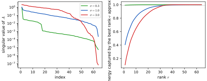
Filling the gap 15.21: random features for softmax attention: unbiasedness, variance, positive features, and the bias of the normalised estimator pp. 535–537, (15.63)–(15.69)
Derivation
(15.64). Put \(\bm q'=\bm q/D^{1/4}\), \(\bm k'=\bm k/D^{1/4}\), so \(\bm q^\T\bm k/\sqrt D=\bm q'^\T\bm k'\). Expanding the square, \(-\frac12\|\bm q'-\bm k'\|^2=\bm q'^\T\bm k'-\frac12\|\bm q'\|^2-\frac12\|\bm k'\|^2\), hence \(\exp(\bm q'^\T\bm k')=e^{\|\bm q'\|^2/2}e^{\|\bm k'\|^2/2}\exp(-\frac12\|\bm q'-\bm k'\|^2)\). With \(\|\bm q'\|^2=\|\bm q\|^2/\sqrt D\) this is (15.64), the last factor being \(K_{\rm gauss}(\bm q',\bm k')\) with \(\sigma=1\).
Trigonometric features (15.65). For \(\bm\omega\sim\N(\bm 0,\bm I_D)\) the characteristic function is \(\E[e^{i\bm\omega^\T\bm u}]=e^{-\|\bm u\|^2/2}\); taking real parts, \(\E[\cos(\bm\omega^\T(\bm x-\bm y))]=e^{-\|\bm x-\bm y\|^2/2}\). Since \(\cos(a-b)=\cos a\cos b+\sin a\sin b\), the feature vector \(\bm\eta(\bm x)=M^{-1/2}[\sin(\bm W\bm x),\cos(\bm W\bm x)]\) built from \(M\) independent rows \(\bm\omega_m\) of \(\bm W\) satisfies \(\E[\bm\eta(\bm x)^\T\bm\eta(\bm y)]=K_{\rm gauss}(\bm x,\bm y)\). Multiplying by \(e^{\|\bm x\|^2/2}\) and \(e^{\|\bm y\|^2/2}\) gives unbiased features for \(\exp(\bm x^\T\bm y)\), and with \(\bm x=\bm q'\), \(\bm y=\bm k'\) this is (15.66), (15.67).
Positive features. Let \(\bm\eta_+(\bm x)=M^{-1/2}\exp(\bm W\bm x-\|\bm x\|^2)\) (elementwise exponential, one entry per row of \(\bm W\)). From the moment generating function of a Gaussian, \(\E[\exp(\bm\omega^\T\bm s)]=\exp(\|\bm s\|^2/2)\), one finds \(\E[\eta_{+,m}(\bm x)\eta_{+,m}(\bm y)]/M^{-1}=e^{-\|\bm x\|^2-\|\bm y\|^2}e^{\|\bm x+\bm y\|^2/2}=e^{-\|\bm x-\bm y\|^2/2}\), again the Gaussian kernel, but now every feature and every estimate \(\bm\phi(\bm q)^\T\bm\phi(\bm k)\) is strictly positive. (The book's (15.67) with \(\bm\eta\) the exponential features of (17.61) is this construction.)
Variance (one feature, \(M=1\)). For the positive estimator \(Z=\exp(\bm\omega^\T\bm s-\frac12(\|\bm x\|^2+\|\bm y\|^2))\), \(\bm s=\bm x+\bm y\): \(\E Z=e^{\bm x^\T\bm y}\) and \(\E Z^2=e^{-\|\bm x\|^2-\|\bm y\|^2}e^{2\|\bm s\|^2}=e^{2\bm x^\T\bm y}e^{\|\bm s\|^2}\), so \[ \var Z=\mathrm{SM}^2\big(e^{\|\bm x+\bm y\|^2}-1\big),\qquad\mathrm{SM}=e^{\bm x^\T\bm y} . \] For the trigonometric estimator \(Z'=e^{(\|\bm x\|^2+\|\bm y\|^2)/2}\cos(\bm\omega^\T(\bm x-\bm y))\), using \(\E\cos^2=\frac12(1+e^{-2\|\bm u\|^2})\) with \(\bm u=\bm x-\bm y\), \[ \var Z'=\mathrm{SM}^2\cdot2\sinh^2\big(\tfrac12\|\bm x-\bm y\|^2\big). \] Both relative variances are divided by \(M\) for \(M\) independent features. The trigonometric one is small when \(\bm x\approx\bm y\) (large attention weight) and grows like \(e^{\|\bm x-\bm y\|^2}\) when the query and key are far apart; the positive one is small when \(\|\bm x+\bm y\|\) is small, which includes the case of strongly opposed query and key, a tiny attention weight. For independent Gaussian queries and keys the two relative variances are of the same order, and in my experiment the trigonometric features were in fact somewhat more accurate for \(M\ge64\) (Figure 15.S7). The decisive difference is the sign: a trigonometric estimate of an attention weight can be negative, so a row sum of \(\bm Q'\bm K'^\T\) can be close to zero or negative and the normalisation in (15.69) then blows up; for queries and keys with standard deviation 0.8 and \(M=16\), 4.9 percent of the rows had a non-positive denominator and the median relative error of the output was 18, against 1.35 for the positive features, whose denominators are always positive. This is the reason for the positive features of Choromanski et al. (2020b). The trigonometric and positive variance formulas were confirmed by simulation (the positive one with \(2\times10^6\) draws, to 5 percent). Orthogonalising the rows of \(\bm W\) within blocks of \(D\) (with chi-distributed norms) keeps each row marginally Gaussian but makes the rows negatively dependent, which lowers the variance further; this is the "orthogonal random features" of the book's parenthesis.
The estimator (15.69) is consistent but not exactly unbiased. The numerator \(\bm Q'(\bm K'^\T\bm V)\) and the denominator \(\bm Q'(\bm K'^\T\bm 1_N)\) are each unbiased for the unnormalised attention \(\bm A\bm V\) and the row sums \(\bm A\bm 1_N\), because \(\E[\bm Q'\bm K'^\T]=\bm A\) and the expression is linear in \(\bm Q'\bm K'^\T\). Their ratio is a nonlinear function: \(\E[X/Y]\ne\E[X]/\E[Y]\) in general, and the bias of a ratio of averages of \(M\) independent copies is \(O(1/M)\) (delta method), so the estimate of softmax attention is consistent as \(M\to\infty\) but not unbiased for finite \(M\). The book's remark that (15.69) "can be shown to be an unbiased approximation" holds for the unnormalised operator. In a small experiment (\(N=6\), \(D=4\)) the relative bias of the normalised output is 0.50 at \(M=2\) and 0.028 at \(M=64\) (averages of \(4\times10^4\) and \(5\times10^3\) draws; standard errors 0.007 and 0.005), and the typical relative error of a single draw falls like \(M^{-1/2}\) (Figure 15.S7). The cost is \(O(NMd)\): for \(N=8192\), \(d=16\), \(M=256\) about \(4NMd=1.3\times10^8\) multiply-adds, against \(2N^2d=2.1\times10^9\) for exact attention. \(\square\)
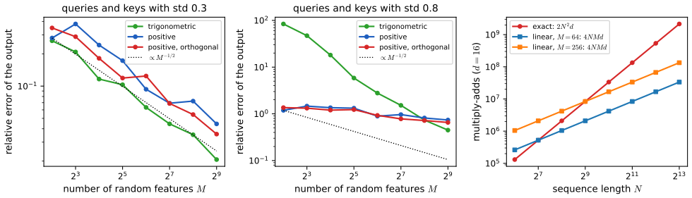
15.7 Language models and unsupervised representation learning
p. 537 RNNs and decoder-only transformers are language models: generative sequence models \(p(x_1,\dots,x_T)=\prod_tp(x_t\given x_{1:t-1})\) over discrete tokens (words or wordpieces; Section 1.5.4 on text preprocessing). Their hidden state \(\bm h_t\), which depends on all earlier tokens, can serve as a contextual embedding of token \(t\) in place of a one-hot vector or a fixed word embedding (Section 20.5), for text classification or seq2seq tasks. The advantage is that the model can be pretrained without labels on a large corpus and then fine-tuned on a small labelled data set (transfer learning, Section 19.2). If one only needs representations, the generative model can be replaced by a non-causal one whose state \(\bm h_t\) depends on the past, the present and the future; this often gives better representations but cannot generate text.
15.7.1 Non-generative language models
pp. 538–542 ELMo (15.7.1.1). Peters et al. (2018) fit two LSTM language models, left-to-right and right-to-left, with shared embedding (\(\theta_e\)) and softmax (\(\theta_s\)) layers (Figure 15.32), by minimising \[ L(\theta)=-\sum_{t=1}^T\Big[\log p(x_t\given x_{1:t-1};\theta_e,\theta_\to,\theta_s)+\log p(x_t\given x_{t+1:T};\theta_e,\theta_\leftarrow,\theta_s)\Big]. \tag{15.70} \] After training, the contextual representation of token \(t\) is \(\bm r_t=[\bm e_t,\bm h^\to_{t,1:L},\bm h^\leftarrow_{t,1:L}]\) (\(L\) the number of LSTM layers), and a task-specific vector \(\bm w^j\) gives \(r_t^j=\bm r_t^\T\bm w^j\): for syntax (part-of-speech tagging) the task puts weight on lower layers, for semantics (word-sense disambiguation) on higher ones, and only the small vector \(\bm w^j\) needs labels.
BERT (15.7.1.2, 15.7.1.3). BERT (Devlin et al., 2019) is a non-causal transformer encoder trained on a modified input to recover the unmodified one: a random set \(m\) of positions is hidden and the task is to predict the missing words from the rest (the cloze or masked language model task). It minimises the negative log pseudo-likelihood
\[ L=\E_{\bm x\sim\mathcal D}\,\E_{m}\sum_{i\in m}-\log p(x_i\given\bm x_{-m}), \tag{15.71} \]
with \(m\) a random binary mask; for instance "Let's make [MASK] chicken! [SEP] It [MASK] great with orange sauce." with targets "some" and "tastes" ([SEP] separates two sentences). With \(\hat{\bm x}=\bm x_{-m}\) the masked input, \(\bm h(\hat{\bm x})_i\) the last-layer vector at position \(i\) and \(\bm e(x)\) the embedding of token \(x\),
\[ p(x_i\given\hat{\bm x})=\frac{\exp(\bm h(\hat{\bm x})_i^\T\bm e(x_i))}{\sum_{x'}\exp(\bm h(\hat{\bm x})_i^\T\bm e(x'))}, \tag{15.72} \]
which resembles a denoising autoencoder (Section 20.3.2). Next sentence prediction (15.7.1.4). BERT was also trained to classify whether sentence \(B\) follows \(A\) in the text (label 1) or is a random sentence (label 0), with input CLS A1 A2 ... Am; SEP B1 B2 ... Bn SEP (15.73). The input is the sum of three embeddings (token, segment A or B, learned position, Figure 15.34); the labels are generated automatically, so the pretraining is self-supervised. Fine-tuning (15.7.1.5). Adding output heads to the final hidden layer solves many tasks (Figure 15.35): sentence classification and sentence-pair classification feed the CLS vector to an MLP; tagging classifies every position (part-of-speech tagging, noun phrase chunking in the BIO notation where B marks the beginning of an entity, I the inside and O the outside, as in "British Airways rose after announcing its withdrawal from the UAI deal": B I O O O B I O B I I; named-entity recognition, with types such as person, location, organisation: "Mrs Green spoke today in New York." has entities "Mrs Green" (person) and "New York" (location)); and question answering applies two MLPs to the encodings of the background text to obtain softmaxes over start and end positions \(s_i\) and \(e_j\), the answer being the span \((i,j)\), \(i\le j\), maximising \(s_i+e_j\). Tenney et al. (2019) found that BERT rediscovers the classical NLP pipeline layer by layer (tagging, parsing, entity recognition, semantic roles, coreference).
Filling the gap 15.22: the masked-language-model objective is a pseudo-likelihood, not the chain rule; why ELMo and BERT avoid leaking the target pp. 538–539, (15.70), (15.71)
Derivation
Chain rule (causal models). For any ordering, \(\log p(\bm x)=\sum_t\log p(x_t\given x_{1:t-1})\), so a causal language model fitted by teacher forcing maximises the exact log-likelihood of a proper joint distribution, and its expected loss is \(H(p^\star)+\KL(p^\star\|p_\theta)\ge H(p^\star)\) (gap 15.4); one can sample from it by ancestral sampling.
Pseudo-likelihood (masked models). The conditionals \(p(x_i\given\bm x_{-m})\) of (15.71) are not the factors of one joint; Besag's (1975) pseudo-log-likelihood \(\sum_i\log p(x_i\given\bm x_{-i})\) is the classical analogue (masking one position at a time). Maximising it is consistent under regularity conditions when the model class contains the truth (Besag, 1975), but nothing forces the learned conditionals to be mutually compatible with one joint distribution, so the model does not define \(p(\bm x)\), cannot be sampled by ancestral sampling, and its loss is not a log-likelihood.
The two losses are not comparable. Let \(\bm x=(x_1,\dots,x_T)\) have a joint distribution \(p\). Since conditioning reduces entropy (Section 6.2, and \(\bm x_{1:t-1}\) is a sub-vector of \(\bm x_{-t}\)), \(H(x_t\given\bm x_{-t})\le H(x_t\given\bm x_{1:t-1})\), so \[ \sum_{t=1}^TH(x_t\given\bm x_{-t})\le\sum_{t=1}^TH(x_t\given\bm x_{1:t-1})=H(\bm x), \] with equality iff \(x_t\) is conditionally independent of the future given the past for every \(t\). The loss of an ideal masked model (the entropy of each token given all others) is therefore lower than that of an ideal causal model: the "pseudo-perplexity" of BERT cannot be compared with the perplexity of GPT. A random joint distribution of three binary variables shows the gap: \(H(\bm x)=1.774\) nats against \(\sum_tH(x_t\given\bm x_{-t})=1.518\) nats. Low pseudo-perplexity does not imply that the model is a good generator.
Leakage. A bidirectional RNN's state at \(t\) contains \(x_t\) itself (it reads \(x_t\) in both directions), so predicting \(x_t\) from it is trivial and teaches nothing. ELMo avoids this by training the two directions as separate language models that share only embedding and softmax parameters, so that each term of (15.70) conditions on one side only: \(L(\theta)=-\log p_\to(\bm x)-\log p_\leftarrow(\bm x)\) is the sum of the exact log-likelihoods of two autoregressive models of the same sequence, one for each order of the chain rule (an exact model would give the same value twice, so the sum is twice the average). BERT instead hides the target (the mask) and lets a bidirectional encoder see everything else; (15.72) is a softmax over the vocabulary with the embedding table as output layer, so its normaliser is a sum over \(|\mathcal V|\) terms and the probabilities sum to one. \(\square\)
15.7.2 Generative (causal) large language models (LLMs)
pp. 542–544 GPT (15.7.2.1). GPT (Radford et al., 2018) is a masked-transformer decoder. In the original paper it was trained on a large unlabelled corpus \(\mathcal D_U\) and a small labelled one \(\mathcal D_L\) jointly, with loss \(L=L_{\rm cls}+\lambda L_{\rm LM}\), \(L_{\rm cls}=-\sum_{(\bm x,y)\in\mathcal D_L}\log p(y\given\bm x)\), \(L_{\rm LM}=-\sum_{\bm x\in\mathcal D_U}\sum_t\log p(x_t\given x_{1:t-1})\). GPT-2 (Radford et al., 2019) is larger, trained on a web corpus (WebText) as a pure language model with no task-specific training; GPT-3 (Brown et al., 2020) and GPT-4 follow the same principles at larger scale; ChatGPT adds reinforcement learning from human feedback (RLHF; Ouyang et al., 2022), in which a ranking model trained on human preferences defines the reward used to fine-tune the model towards responses aligned with human intent. Larger models trained on more data do better at next-word prediction and downstream tasks (the scaling hypothesis, Kaplan et al., 2020). Applications (15.7.2.2). An LLM generates text from a prompt; if the answer fulfils the task without any training on it, one has zero-shot transfer (Section 19.6). For example, abstractive summarisation samples \(p(x_{T+1:T+100}\given[x_{1:T};\text{TL;DR}])\), where the token "TL;DR" frequently precedes a human summary in web text (an example of prompt engineering); training on input-output pairs is arguably a better way to specify the task. LLMs also serve as chatbots and code generators. T5 (15.7.2.3). A single seq2seq transformer can be trained on many tasks by writing the task into the input (Raffel et al., 2020): "translate English to German: That is good." gives "Das ist gut." (Figure 15.36). T5 is pretrained with a BERT-like denoising objective on the colossal clean crawled corpus C4 (750 GB): "Thank you for inviting me to your party last week" becomes the input "Thank you <X> me to your party <Y> week" and the target "<X> for inviting <Y> last <EOS>", with sentinel tokens unique to the example; it is then fine-tuned on supervised pairs, and FLAN-T5 (Chung et al., 2022) uses instruction fine-tuning on over 1800 tasks. Discussion (15.7.2.4). It is debated whether such systems understand language and reasoning or merely exploit superficial patterns in their massive training sets (Dziri et al., 2024; Narayanan and Kapoor, 2024).
Exercises
This chapter of the book has no end-of-chapter exercises (checked in the April 2025 draft). The eight exercises below are my own, in the spirit of the notes; each has a complete worked solution (hidden), computational ones solved with the code of this chapter.
Exercise 15.1 (perplexity). (a) A language model assigns the conditional probabilities \(0.5,0.25,0.125,0.125\) to the four tokens of a sequence. Compute its perplexity and the number of bits per token. (b) The character GRU of Figure 15.2 has held-out perplexity 4.37 on a 28-symbol alphabet. What is its bits-per-character, and how many bits does a uniform model need?
Solution
(a) \(\operatorname{PPL}=(0.5\cdot0.25\cdot0.125\cdot0.125)^{-1/4}=(2^{-9})^{-1/4}=2^{9/4}=4.757\); the log-loss is \(9/4=2.25\) bits per token. (b) \(\log_24.37=2.13\) bits per character; a uniform model needs \(\log_228=4.81\) bits (perplexity 28). The GRU removes 2.7 of the 4.8 bits.
Exercise 15.2 (BPTT on a scalar RNN). Let \(h_t=wh_{t-1}+x_t\), \(h_0=0\), \(T=3\) and \(L=\frac12(h_3-y)^2\). (a) Evaluate \(\partial h_3/\partial w\) with (15.22). (b) For \(w=0.5\), \(\bm x=(1,2,-1)\), \(y=0\), find \(\partial L/\partial w\) and check it by the backward recursion of gap 15.5.
Solution
(a) Here \(f(x_t,h_{t-1},w)=wh_{t-1}+x_t\), so \(\bm J_j=w\) and \(\bm F_i=h_{i-1}\): \(\bm F_1=0\), \(\bm F_2=h_1=x_1\), \(\bm F_3=h_2=wx_1+x_2\). Then (15.22) gives \(\partial h_3/\partial w=F_3+J_3F_2+J_3J_2F_1=(wx_1+x_2)+wx_1+0=2wx_1+x_2\), in agreement with differentiating \(h_3=w^2x_1+wx_2+x_3\). (b) \(h_3=0.25+1-1=0.25\), \(\partial h_3/\partial w=1+2=3\), so \(\partial L/\partial w=(h_3-y)\cdot3=0.75\). Backward: \(\delta_3=h_3-y=0.25\), \(\delta_2=w\delta_3=0.125\), \(\delta_1=w\delta_2=0.0625\); \(\partial L/\partial w=\sum_tF_t\delta_t=0\cdot0.0625+x_1\cdot0.125+(wx_1+x_2)\cdot0.25=0.125+0.625=0.75\). Both agree with a finite-difference derivative.
Exercise 15.3 (forget-gate bias). An LSTM cell with constant forget gate \(f=\sigma(b)\) and no input keeps a fraction \(f^k\) of its memory after \(k\) steps. (a) What bias gives a half-life of 100 steps? (b) What half-life does \(b=2\) give? (c) What does the default \(b=0\) give?
Solution
(a) \(f^{100}=\frac12\Rightarrow f=2^{-1/100}=0.99309\Rightarrow b=\operatorname{logit}f=\ln\frac{f}{1-f}=4.968\). (b) \(\sigma(2)=0.8808\), half-life \(=\ln2/(-\ln0.8808)=5.46\) steps. (c) \(\sigma(0)=0.5\): half-life 1 step. That is why the delayed-recall experiment fails for LSTMs trained from a default initialisation.
Exercise 15.4 (designing a receptive field). A causal convolutional model must see the last 1000 samples. How many layers are needed with (a) kernel size 2 and dilations \(1,2,4,\dots\); (b) kernel size 3 and dilations \(1,3,9,\dots\)? Compare the parameters for \(C=64\) channels in and out (ignoring biases).
Solution
By gap 15.12, \(R=1+(k-1)\sum d_l\). (a) \(R=1+\sum_{l=0}^{L-1}2^l=2^L\ge1000\Rightarrow L=10\) (\(R=1024\)); parameters \(10\cdot2\cdot64^2=81{,}920\). (b) \(R=1+2\sum_{l=0}^{L-1}3^l=3^L\ge1000\Rightarrow L=7\) (\(R=2187\)); parameters \(7\cdot3\cdot64^2=86{,}016\). The wider kernel needs three fewer layers (less depth, less sequential latency) for about 5 percent more parameters.
Exercise 15.5 (scaling the scores). Draw \(\bm q\) and ten keys with independent \(\N(0,1)\) entries in \(\R^d\), and compute softmax attention weights from \(\bm q^\T\bm k_j\) and from \(\bm q^\T\bm k_j/\sqrt d\). Report the mean largest weight and the mean entropy over 20,000 draws for \(d=4,16,64,256\), and explain.
Solution
Simulation (the maximum possible entropy is \(\ln10=2.303\)):
\(d\) largest weight, unscaled entropy, unscaled largest weight, scaled entropy, scaled 4 0.493 1.436 0.305 1.948 16 0.727 0.748 0.315 1.934 64 0.866 0.346 0.320 1.923 256 0.935 0.162 0.321 1.921 Unscaled scores have standard deviation \(\sqrt d\) (gap 15.15), so the weights collapse onto one key as \(d\) grows (entropy 0.16 at \(d=256\)); scaled scores have standard deviation 1 for all \(d\), and the distribution of the weights does not depend on \(d\) (largest weight about 0.32, entropy about 1.92).
Exercise 15.6 (a small positional code). Take \(d=4\) and \(C=100\). (a) Write \(\bm p_t\). (b) Show that \(\bm p_t^\T\bm p_{t+\phi}=\cos\phi+\cos(\phi/10)\), and evaluate it at \(\phi=0,1,\pi\). (c) Find \(\bm R(\phi)\) with \(\bm p_{t+\phi}=\bm R(\phi)\bm p_t\).
Solution
(a) \(\omega_0=C^0=1\), \(\omega_1=C^{-2/4}=0.1\): \(\bm p_t=(\sin t,\cos t,\sin(t/10),\cos(t/10))\). (b) By gap 15.17, \(\bm p_t^\T\bm p_{t+\phi}=\sum_k\cos(\omega_k\phi)=\cos\phi+\cos(\phi/10)\); the values are \(2\) (\(=d/2\)), \(0.5403+0.9950=1.5353\) and \(-1+0.9511=-0.0489\). (c) \(\bm R(\phi)=\operatorname{blockdiag}\big(\begin{pmatrix}\cos\phi&\sin\phi\\-\sin\phi&\cos\phi\end{pmatrix},\begin{pmatrix}\cos(\phi/10)&\sin(\phi/10)\\-\sin(\phi/10)&\cos(\phi/10)\end{pmatrix}\big)\), the same for all \(t\).
Exercise 15.7 (causal linear attention as an RNN). For feature maps \(\bm\phi\in\R^M\) and values in \(\R^d\), write the causal linear attention output as a recurrence with a matrix state. How many numbers does the state hold, and how does this compare with the key-value cache of softmax attention for \(N=4096\), \(M=64\), \(d=64\)?
Solution
As in gap 15.20: \(\bm S_t=\bm S_{t-1}+\bm\phi(\bm k_t)\bm v_t^\T\), \(\bm z_t=\bm z_{t-1}+\bm\phi(\bm k_t)\), \(\bm y_t=\bm\phi(\bm q_t)^\T\bm S_t/(\bm\phi(\bm q_t)^\T\bm z_t)\). The state \((\bm S_t,\bm z_t)\) has \(M(d+1)=64\cdot65=4160\) numbers, independent of \(t\); the update and the read-out each cost \(O(Md)\). A softmax key-value cache holds \(2Nd=2\cdot4096\cdot64=524{,}288\) numbers at the end of the sequence (and grows with \(t\)), 126 times more.
Exercise 15.8 (beam search). (a) Show that beam search with \(K\ge V\) is exact when \(T=2\). (b) In the example of gap 15.10 explain in one sentence why \(K=2\) loses the best path and \(K=3\) does not, and compute the three results.
Solution
(a) With \(K\ge V\) the beam after step 1 contains all \(V\) one-token prefixes, and step 2 expands all of them, so every sequence of length 2 is a candidate; the best one is returned. (b) With \(K=2\) two children of the second-best first token outrank every child of the best first token (\(0.15,0.15\) against \(0.136\)), so the prefix \(a\) is pruned at step 2; with \(K=3\) the third slot keeps \(aa\). The results are \(K=1\): \(0.1224\); \(K=2\): \(0.051\); \(K=3\): \(0.1224\) (the exact maximum, by enumeration).
Demonstrations
| Page | What it shows | In the notes |
|---|---|---|
| Gradient flow in recurrent cells | The norm \(\|\partial\bm s_T/\partial\bm s_{T-k}\|_2\) against the lag for a linear RNN, a tanh RNN, a GRU and an LSTM with adjustable spectral radius, weight scale and gate bias. Presets: 1 vanishing (\(\rho=0.8\)); 2 exploding (\(\rho=1.2\)); 3 tanh saturates; 4 all cells, gate bias 0; 5 gate bias 4. | 15.2.6, 15.2.7, gap 15.6, gap 15.8, gap 15.9 |
| Decoding a character model | The trained GRU of Figure 15.2 generating text by greedy decoding, temperature sampling and beam search, with the log-probability of the result; and the beam-search trees of Figures 15.12 and 15.13. Presets: 1 greedy; 2 temperature 0.8; 3 temperature 1.6; 4 beam width 4; 5 the book's toy tree. | 15.2.1, 15.2.8, gap 15.2, gap 15.10 |
| Kernel regression as attention | Nadaraya–Watson regression with a Gaussian kernel written as softmax attention: the attention matrix, the fit, the attention row of a probe point and the leave-one-out score against \(\beta\). Presets: 1 \(\beta=1\) (Figure 15.17); 2 oversmoothed; 3 overfit; 4 leave-one-out choice; 5 few noisy points. | 15.4.2, gap 15.14 |
| Positional encoding and attention scores | The sinusoidal code (heat map, similarity against the offset, the rotation property), the binary code, and the distribution of dot-product scores and attention weights with and without \(1/\sqrt d\). Presets: 1 Figure 15.25; 2 binary code; 3 rotation property; 4 small \(C\); 5 score scaling. | 15.4.3, 15.5.3, gap 15.15, gap 15.17 |
The Python code that produces every figure of this page is code/ch15_neural_networks_sequences.py (see the code index). Companion demos: attention explorer, character-level transformer, sampling strategies, permutation equivariance.
Notes on the book
Points where the book is imprecise or wrong
- Section 15.2.8, Figure 15.12. With the vocabulary \((A,B,C,\eos)\) and \(p(y_2\given A)=[0.1,0.4,0.3,0.2]\) the short sequence \((A,\eos)\) has probability \(0.5\times0.2=0.1\), larger than the two sequences compared (0.048 and 0.054). The example does show that greedy decoding is not the MAP sequence, but the MAP sequence of these tables is \((A,\eos)\) (gap 15.10).
- Section 15.2.8, beam search. Wider beams do not always help: the score of the returned sequence is not monotone in the beam width (explicit example in gap 15.10). Comparing hypotheses of different length by total log-probability favours short ones.
- Section 15.3.2, (15.33). As printed, \(\sum_{\tau=1}^{t-k}\bm w^\T\bm y_{\tau:\tau+k}\) adds the responses of all windows ending before \(t\), which is a global sum rather than a convolution of width \(k\); a causal convolution with a fixed receptive field uses the single window \(\bm y_{t-k:t-1}\) (gap 15.12).
- Section 15.5.3, "attention is permutation invariant". Self-attention is permutation equivariant: permuting the inputs permutes the outputs in the same way (gap 15.13(c)); the output is invariant only after an order-insensitive pooling.
- (15.59), (15.60). The second row of (15.59) writes \(\sin(\omega t)\sin(\omega_k\phi)\) with the index \(k\) missing in one frequency. Also, the sentence "if \(\phi\) is small then \(\bm p_{t+\phi}\approx\bm p_t\)" holds only for the slowly varying coordinates: for \(\omega_0=1\) a shift of one position already changes the first pair by 0.96, and for \(d=32\) neighbouring codes differ by 1.17 against a norm of 4 (gap 15.17).
- Section 15.5.5, "for short sequences \(n\ll d\)". Attention is cheaper than a recurrent layer iff \(2n^2d<2nd^2\), i.e. iff \(n<d\) (the projections add \(4nd^2\) to attention, which is lower order only for \(n>d\)) (gap 15.18).
- Section 15.6.4, "\(M<D\)" and \(M=O(D\log D)\). The text asks for a feature dimension \(M<D\) after (15.62) and later takes \(M=O(D\log D)\), which exceeds \(D\). What is needed for a saving is \(M\ll N\), the sequence length (the rank of \(\bm Q'\bm K'^\T\) is at most \(M\)); \(D\) is the dimension of the keys. (This is how I read the text; the surrounding discussion is about \(N\).)
- Section 15.6.4, (15.69), "unbiased". The numerator and denominator of (15.69) are unbiased estimates of the unnormalised attention and of its row sums; the normalised ratio is consistent but biased for finite \(M\) (relative bias about 0.5 at \(M=2\) and 0.03 at \(M=64\) in a small experiment, gap 15.21).
- Section 15.7.1.3, (15.71). The masked-language-model loss is a pseudo-likelihood, not a log-likelihood, and its values are lower than the causal language-modelling loss even for an ideal model (gap 15.22), so the two are not comparable.
References
- Murphy, K. P. (2022). Probabilistic Machine Learning: An Introduction. MIT Press, Cambridge, MA. Chapter 15, pp. 503–544. probml.github.io/pml-book/book1.html.
- Bahdanau, D., Cho, K. and Bengio, Y. (2015). Neural machine translation by jointly learning to align and translate. International Conference on Learning Representations.
- Bengio, S., Vinyals, O., Jaitly, N. and Shazeer, N. (2015). Scheduled sampling for sequence prediction with recurrent neural networks. Advances in Neural Information Processing Systems, 28.
- Besag, J. (1975). Statistical analysis of non-lattice data. The Statistician, 24(3), 179–195.
- Brown, T. B. et al. (2020). Language models are few-shot learners. Advances in Neural Information Processing Systems, 33.
- Carroll, L. (1865). Alice's Adventures in Wonderland (public domain text used for the character models).
- Choromanski, K. et al. (2021). Rethinking attention with Performers. International Conference on Learning Representations.
- Dai, Z. et al. (2019). Transformer-XL: attentive language models beyond a fixed-length context. Proceedings of the Association for Computational Linguistics.
- Devlin, J., Chang, M.-W., Lee, K. and Toutanova, K. (2019). BERT: pre-training of deep bidirectional transformers for language understanding. Proceedings of NAACL-HLT.
- Dosovitskiy, A. et al. (2021). An image is worth 16x16 words: transformers for image recognition at scale. International Conference on Learning Representations.
- Gumbel, E. J. (1954). Statistical Theory of Extreme Values and Some Practical Applications. National Bureau of Standards.
- Hochreiter, S. and Schmidhuber, J. (1997). Long short-term memory. Neural Computation, 9(8), 1735–1780.
- Jaeger, H. and Haas, H. (2004). Harnessing nonlinearity: predicting chaotic systems and saving energy in wireless communication. Science, 304(5667), 78–80.
- Jozefowicz, R., Zaremba, W. and Sutskever, I. (2015). An empirical exploration of recurrent network architectures. International Conference on Machine Learning.
- Katharopoulos, A., Vyas, A., Pappas, N. and Fleuret, F. (2020). Transformers are RNNs: fast autoregressive transformers with linear attention. International Conference on Machine Learning.
- Kim, Y. (2014). Convolutional neural networks for sentence classification. Proceedings of EMNLP.
- Kool, W., van Hoof, H. and Welling, M. (2019). Stochastic beams and where to find them: the Gumbel-top-k trick for sampling sequences without replacement. International Conference on Machine Learning.
- Luce, R. D. (1959). Individual Choice Behavior. Wiley, New York.
- Luong, M.-T., Pham, H. and Manning, C. D. (2015). Effective approaches to attention-based neural machine translation. Proceedings of EMNLP.
- Maass, W., Natschläger, T. and Markram, H. (2002). Real-time computing without stable states. Neural Computation, 14(11), 2531–2560.
- Parikh, A. P., Täckström, O., Das, D. and Uszkoreit, J. (2016). A decomposable attention model for natural language inference. Proceedings of EMNLP.
- Peters, M. E. et al. (2018). Deep contextualized word representations. Proceedings of NAACL-HLT.
- Plackett, R. L. (1975). The analysis of permutations. Applied Statistics, 24(2), 193–202.
- Radford, A. et al. (2018, 2019). Improving language understanding by generative pre-training; Language models are unsupervised multitask learners. OpenAI technical reports.
- Raffel, C. et al. (2020). Exploring the limits of transfer learning with a unified text-to-text transformer. Journal of Machine Learning Research, 21(140), 1–67.
- Rahimi, A. and Recht, B. (2007). Random features for large-scale kernel machines. Advances in Neural Information Processing Systems, 20.
- Schuster, M. and Paliwal, K. K. (1997). Bidirectional recurrent neural networks. IEEE Transactions on Signal Processing, 45(11), 2673–2681.
- Tenney, I., Das, D. and Pavlick, E. (2019). BERT rediscovers the classical NLP pipeline. Proceedings of the Association for Computational Linguistics.
- van den Oord, A. et al. (2016). WaveNet: a generative model for raw audio. arXiv:1609.03499.
- Vaswani, A. et al. (2017). Attention is all you need. Advances in Neural Information Processing Systems, 30.
- Wang, S., Li, B. Z., Khabsa, M., Fang, H. and Ma, H. (2020). Linformer: self-attention with linear complexity. arXiv:2006.04768.
- Xu, K. et al. (2015). Show, attend and tell: neural image caption generation with visual attention. International Conference on Machine Learning.
The numerical statements in the text (the normalisation of the RNN likelihood, the KL decomposition and the total-variation bound for teacher forcing, the backward recursion and the explicit sum for backpropagation through time, the norm bounds and the clipping projection, the echo state contraction, the GRU limits and Jacobian, the LSTM against a standard library and its cell-path derivative, the forget-gate time constants, the beam-search examples and the non-monotone case, the Gumbel and Plackett–Luce frequencies, the causal convolutions and receptive fields, the attention identities, the Nadaraya–Watson equivalences, the variance of dot-product scores, multi-head attention against a library, the positional-code identities, parallel against incremental decoding, the cost counts, the patch-embedding convolution, the block-local and linear attention identities, the random-feature means and variances, and the numerical answers to the exercises) were confirmed numerically.