Graph Neural Networks
Sequences and images are data on a line and on a grid. Many data sets live on a general graph instead: atoms joined by bonds, people joined by friendships, papers joined by citations. To store a graph we must number its nodes, and the numbering is arbitrary, so a network for graphs must give answers that do not depend on it: node-level outputs must be reordered along with the nodes (equivariance) and graph-level outputs must not change at all (invariance). This chapter builds such networks from one idea, neural message passing: every node repeatedly collects its neighbours' vectors with a symmetric function and updates its own vector with weights shared by all nodes (Section 13.2). Section 13.1 sets up graphs, adjacency matrices and permutation matrices; Section 13.3 adds attention, edge and graph embeddings, explains over-smoothing, and ends with networks that also respect rotations and translations of space.
Ch. 1 Deep learning revolution Ch. 2 Probabilities Ch. 3 Standard distributions Ch. 4 Regression Ch. 5 Classification Ch. 6 Deep neural networks Ch. 7 Gradient descent Ch. 8 Backpropagation Ch. 9 Regularization Ch. 10 Convolutional networks Ch. 11 Structured distributions Ch. 12 Transformers Ch. 13 Graph neural networks Ch. 14 Sampling Ch. 15 Discrete latent variables Ch. 16 Continuous latent variables Ch. 17 GANs Ch. 18 Normalizing flows Ch. 19 Autoencoders Ch. 20 Diffusion models Appendices A to C
How to read these notes
They follow the book. Sections carry the book's numbers (13.1, 13.2.3, ...) and every displayed equation that appears in the book carries the book's own equation number, e.g. (13.16), so the notes can be read next to the book. Equations without a number are steps that the book skips.
Filling the gaps. The chapter states many properties in words: that a layer "is clearly" equivariant, that the mean is "provably less powerful" than the sum, that (13.15) is a universal approximator, that residual connections help against over-smoothing. Each such statement gets an orange Filling the gap box or a result with a complete proof. Proofs and derivations start hidden: open one with its bar, or use the button below.
Figures and demonstrations. Of the chapter's five figures, three (13.2, 13.3, 13.4) are computed here by the Python code; Figure 13.1 (drawings of a molecule, a rail map and web pages) and Figure 13.5 (a schematic of which variables enter which update) have nothing to compute. Seven supplementary figures (13.S1 to 13.S7, our own) illustrate the gaps that are filled. The ▶ Demo boxes open an interactive demonstration already set to the case being discussed.
Main reference
C. M. Bishop and H. Bishop, Deep Learning: Foundations and Concepts, Springer (2024), Chapter 13, pages 407–427. Section, equation, figure and exercise numbers below refer to this book. Further reading is listed in the references; the book's website is www.bishopbook.com. The book has no official solutions for this chapter; the solutions to the exercises below are my own.
The explanations, derivations, figures and code are my own; equations are cited by their numbers in the book.
Companion course: Bayesian and Probabilistic Machine Learning
Graph neural networks are new relative to Bishop (2006), but several ingredients appear in the companion course Bayesian and Probabilistic Machine Learning, and these notes link them where they arise.
- Undirected graphs, neighbourhoods and cliques: Section 8.3 (Markov random fields), and an image as a grid graph of pixels in Section 8.3.3 (here 13.1.1 and 13.2.1).
- Message passing on a graph, with a synchronous "flooding" schedule on graphs with loops: the sum-product algorithm and loopy belief propagation (here 13.2.2). There the messages are fixed by probability theory; here they are learned.
- Invariance built into a model, weight sharing and convolutional networks: Section 5.5.3, Section 5.5.5 (augmentation) and Section 5.5.6 (here 13.1.2 and 13.2.1).
- The softmax output and cross-entropy of multiclass logistic regression, Section 4.3.4, and backpropagation, Section 5.3 (here 13.2.5).
- Demonstrations: the sum-product demo, the image de-noising demo (local updates on a pixel graph) and the backpropagation demo.
The chapter at a glance
- 13.1 A graph with \(N\) nodes is stored as node data \(\bX\) and an adjacency matrix \(\bA\). Reordering the nodes by a permutation matrix \(\bP\) gives \(\bP\bX\) and \(\bP\bA\bP^\T\) (Result 13.1). A graph has \(N!/|\mathrm{Aut}|\) different adjacency matrices, which is why a network on the flattened \(\bA\) is hopeless (Filling the gap 13.1).
- 13.2 Message passing with a symmetric aggregation and a shared update is equivariant, and a sum, mean or max readout is invariant (Result 13.2). Sum aggregation can count, mean and max cannot (Result 13.3); sums of learned features can represent every continuous function of a set (Filling the gap 13.5). The normalised matrices have spectra in \([0,2]\) and \((-1,1]\) (Result 13.4); \(L\) layers see exactly the \(L\)-hop neighbourhood (Result 13.5). The gradients of a GCN node classifier in matrix form, and why unlabelled nodes still learn (13.8, 13.9).
- 13.3 Attention gives data-dependent neighbour weights and, on a complete graph with self-loops, is a transformer (Result 13.7). Repeated normalised averaging converges to the leading eigenvector at rate \(\rho^k\), and ReLU layers shrink the Dirichlet energy by \(\rho^2\|\bW\|^2\) (over-smoothing, Results 13.9 and 13.10); what residual connections do (Result 13.11). The E(n)-equivariant layer (13.38)–(13.41) (Result 13.12).
Notation. \(\cG=(\cV,\cE)\) is a graph with nodes \(n=1,\dots,N\); \(\nb(n)\) the neighbours of \(n\); \(d_n=|\nb(n)|\) its degree and \(\bD=\diag(d_1,\dots,d_N)\). \(\bA\) is the adjacency matrix, \(\tA=\bA+\bI\), \(\tD=\bD+\bI\), and \(\Ah=\tD^{-1/2}\tA\tD^{-1/2}\) the GCN propagation matrix. Node vectors are columns \(\bx_n,\bh_n\in\R^D\); matrices \(\bX,\bH\) have them as rows. \(\bP\) is a permutation matrix and \(\pi\) its permutation. \(\one_N\) is the all-ones vector of length \(N\).
Printings. The first printing has a missing logarithm in the loss (13.21), a wrong dimension in Exercise 13.6, and a few statements that need a qualification (the description of \(\bP\), the deep-sets remark, the transformer equivalence). Each is flagged where it occurs, and the list with the evidence is in the summary before the exercises.
pp. 407–408 A graph is a set of objects (nodes) and a set of links between pairs of them (edges); both may carry data. In a molecule the nodes are atoms with a type and the edges are bonds with a type; in a rail network the edges may carry travel times; on the web the edges are hyperlinks, which have a direction. Other examples are protein interaction networks, electrical circuits, social networks and the knowledge graph of an organisation, with several kinds of nodes and edges. An image is a graph too: pixels joined to their neighbours. Convolutional networks (Chapter 10 of the book) exploit that particular graph, with translation equivariance built in; graph neural networks generalise the idea to any graph, and the symmetry to build in becomes the freedom to renumber the nodes.
13.1 Machine Learning on Graphs
p. 409 Prediction tasks on graphs come in three kinds. Node tasks predict a property of each node (the topic of a document from its citations). Edge tasks predict a property of a pair of nodes, most often whether an edge should exist (edge prediction or graph completion: unknown protein interactions); finding communities in a known graph also belongs here. Graph tasks predict a property of a whole graph (is a molecule soluble?), from a training set of graphs regarded as independent draws from a common distribution: graph regression or classification.
Graph-level tasks are inductive: the test graphs are new. Node tasks are often transductive: the whole graph is known, a few nodes are labelled, and the goal is to label the rest (separating real people from bots in a social network), a form of semi-supervised learning. Graph networks can also be trained to produce representations for later tasks, for instance a foundation model of molecules fine-tuned on a small labelled set (representation and transfer learning, Sections 6.3.3 and 6.3.4). In every case the network keeps an embedding vector per node, initialised with the node's data and refined layer by layer, much as a transformer refines token embeddings (Chapter 12 of the book); edges and the whole graph may carry embeddings too.
13.1.1 Graph properties
See also the companion course, Section 8.3, where undirected graphs describe conditional independences instead of computations.
p. 410 The chapter works with simple graphs: undirected edges, at most one edge between two nodes, and no self-edges.
Definition 13.1 (graph, neighbours, degree, walks, distance) p. 410
A graph \(\cG=(\cV,\cE)\) has nodes \(\cV=\{1,\dots,N\}\) and edges \(\cE\), each an unordered pair \(\{n,m\}\) with \(n\ne m\) (written \((n,m)\)). Linked nodes are neighbours; \(\nb(n)\) is the set of neighbours of \(n\) and \(d_n=|\nb(n)|\) its degree. Node \(n\) carries data \(\bx_n\in\R^D\), and \(\bX\in\R^{N\times D}\) has rows \(\bx_n^\T\). A walk of length \(k\) is a sequence of nodes \(n_0,\dots,n_k\) with consecutive nodes linked; the distance \(\dist(n,m)\) is the length of a shortest walk between them (\(\infty\) if there is none), and the diameter is the largest finite distance. A graph is connected if every distance is finite, and bipartite if its nodes split into two sets with every edge running between them (equivalently, it has no cycle of odd length).
13.1.2 Adjacency matrix
pp. 410–411 Number the nodes \(1,\dots,N\). The adjacency matrix \(\bA\in\{0,1\}^{N\times N}\) has \(A_{nm}=1\) if there is an edge from \(n\) to \(m\) and \(0\) otherwise; for undirected graphs it is symmetric, \(A_{nm}=A_{mn}\), and for simple graphs its diagonal is zero. Its row sums are the degrees, \(d_n=\sum_mA_{nm}\), and its powers count walks: \((\bA^k)_{nm}\) is the number of walks of length \(k\) from \(n\) to \(m\) (expand the matrix product: each term \(A_{nn_1}A_{n_1n_2}\cdots A_{n_{k-1}m}\) is 1 exactly for a walk). So \(\diag(\bA^2)\) gives the degrees (Exercise 13.2) and \(\Tr(\bA^3)/6\) the number of triangles (45 in the karate club used below; checked).
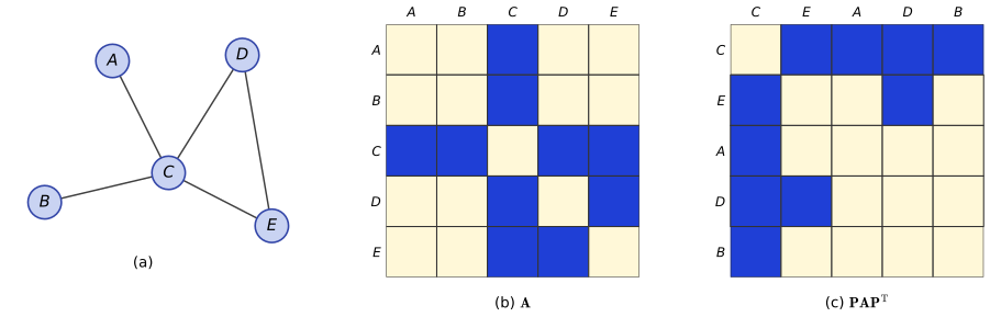
fig_13_2. Reproduces Bishop and Bishop (2024), Figure 13.2. Download: PDF · SVGp. 411 Why not feed \(\vec(\bA)\), the columns of \(\bA\) stacked into one vector, to an ordinary network? Because \(\bA\) depends on the numbering. A molecule's solubility does not, and the number of numberings grows factorially, so learning the invariance from data or from augmentation (randomly renumbered copies, see Section 5.5.5 of the companion course) is hopeless. The invariance must be built into the architecture as an inductive bias.
Filling the gap 13.1: how many adjacency matrices one graph has, and what a network on \(\vec(\bA)\) would have to learn p. 411
The book says the number of permutations "increases factorially". Here is the exact count of different-looking adjacency matrices, and the cost of making a generic network invariant.
Derivation
Counting. The \(N!\) permutation matrices act on adjacency matrices by \(\bA\mapsto\bP\bA\bP^\T\) (Result 13.1 below shows this is a group action: \(\bP_1(\bP_2\bA\bP_2^\T)\bP_1^\T=(\bP_1\bP_2)\bA(\bP_1\bP_2)^\T\)). The set of matrices reachable from \(\bA\) is its orbit; the permutations that fix \(\bA\), \(\bP\bA\bP^\T=\bA\), form its stabiliser, the automorphism group \(\mathrm{Aut}(\cG)\). Two permutations give the same matrix iff \(\bP_1\bA\bP_1^\T=\bP_2\bA\bP_2^\T\), i.e. iff \(\bP_2^\T\bP_1\in\mathrm{Aut}(\cG)\), i.e. iff they lie in the same left coset of \(\mathrm{Aut}(\cG)\). The cosets all have \(|\mathrm{Aut}(\cG)|\) elements, so \[ \#\{\bP\bA\bP^\T\}=\frac{N!}{|\mathrm{Aut}(\cG)|}. \] For the graph of Figure 13.2, swapping \(A\leftrightarrow B\) and/or \(D\leftrightarrow E\) fixes \(\bA\), so \(|\mathrm{Aut}|=4\) and there are \(120/4=30\) different matrices; for the graph of Exercise 13.3, \(|\mathrm{Aut}|=2\) and there are 60 (both counted by brute force). Most large graphs have no symmetry at all, and then all \(N!\) matrices differ: for the 34-member karate club, \(34!\approx3\times10^{38}\).
A network on \(\vec(\bA)\). An ordinary network \(f(\vec(\bA))\) is invariant only if it takes the same value on all \(N!/|\mathrm{Aut}|\) points of every orbit. A random network does not: on the graph of Figure 13.2 a small fully connected network gives 30 different outputs, one per orbit point (Figure 13.S1). One can force invariance by averaging over all orders, \(\bar f(\bA)=\frac1{N!}\sum_{\bP}f(\vec(\bP\bA\bP^\T))\), which is invariant because reordering \(\bA\) merely permutes the terms of the sum, but it costs \(N!\) evaluations. Message passing achieves invariance at a cost linear in the number of edges. ∎
13.1.3 Permutation equivariance
pp. 411–412 A renumbering is described by a permutation matrix \(\bP\): an \(N\times N\) matrix with a single 1 in each row and each column. With unit vectors \(\bu_n\) (1 in position \(n\), zeros elsewhere) the identity is
\[ \bI=\begin{pmatrix}\bu_1^\T\\ \bu_2^\T\\ \vdots\\ \bu_N^\T\end{pmatrix}, \tag{13.2} \]and for a permutation function \(\pi\) of \(\{1,\dots,N\}\)
\[ \bP=\begin{pmatrix}\bu_{\pi(1)}^\T\\ \bu_{\pi(2)}^\T\\ \vdots\\ \bu_{\pi(N)}^\T\end{pmatrix}. \tag{13.3} \]The reordering \((A,B,C,D,E)\to(C,E,A,D,B)\) of Figure 13.2 has \(\pi=(3,5,1,4,2)\) and
\[ \bP=\begin{pmatrix}0&0&1&0&0\\0&0&0&0&1\\1&0&0&0&0\\0&0&0&1&0\\0&1&0&0&0\end{pmatrix}. \tag{13.1} \]Reordering the nodes permutes the rows of the data matrix and both the rows and the columns of the adjacency matrix:
\[ \widetilde\bX=\bP\bX, \tag{13.4} \] \[ \widetilde\bA=\bP\bA\bP^\T. \tag{13.5} \]Result 13.1 (permutation matrices) pp. 411–412, (13.3)–(13.5); Exercises 13.1, 13.4, 13.5
Let \(\bP\) be given by (13.3), so \(P_{nm}=1\) iff \(m=\pi(n)\). Then
- \(\bP\bP^\T=\bP^\T\bP=\bI\): \(\bP\) is orthogonal and \(\bP^{-1}=\bP^\T\) (the matrix of \(\pi^{-1}\)); \(\det\bP=\pm1\).
- Row \(n\) of \(\bP\bX\) is row \(\pi(n)\) of \(\bX\): \((\bP\bX)_{nj}=X_{\pi(n)j}\). Row \(n\) of the reordered data holds the old node \(\pi(n)\).
- \((\bP\bA\bP^\T)_{nm}=A_{\pi(n)\pi(m)}\): new nodes \(n\) and \(m\) are linked iff old nodes \(\pi(n)\) and \(\pi(m)\) were.
- If \(\bP_\sigma,\bP_\pi\) are the matrices of \(\sigma,\pi\), then \(\bP_\sigma\bP_\pi=\bP_{\pi\circ\sigma}\): two reorderings in a row are one reordering.
Proof
(1) \((\bP\bP^\T)_{nm}=\bu_{\pi(n)}^\T\bu_{\pi(m)}=\delta_{\pi(n)\pi(m)}=\delta_{nm}\) because \(\pi\) is one-to-one; \(\bP^\T\bP=\sum_n\bu_{\pi(n)}\bu_{\pi(n)}^\T=\sum_k\bu_k\bu_k^\T=\bI\) because \(\pi\) is onto. Then \(\det(\bP)^2=\det(\bP\bP^\T)=1\).
(2) \((\bP\bX)_{nj}=\sum_mP_{nm}X_{mj}=X_{\pi(n)j}\), since only \(m=\pi(n)\) contributes.
(3) \[(\bP\bA\bP^\T)_{nm}=\sum_{k,l}P_{nk}A_{kl}P_{ml}=A_{\pi(n)\pi(m)},\] since only \(k=\pi(n)\), \(l=\pi(m)\) contribute. In words, \(\bP\bA\) permutes the rows and \(\bA\bP^\T=(\bP\bA^\T)^\T\) the columns.
(4) \((\bP_\sigma\bP_\pi\bX)_n=(\bP_\pi\bX)_{\sigma(n)}=\bx_{\pi(\sigma(n))}^\T\) for every \(\bX\), which is the action of \(\bP_{\pi\circ\sigma}\).
Exercise 13.1. With \(\pi=(3,5,1,4,2)\) the rows of (13.3) are \(\bu_3^\T,\bu_5^\T,\bu_1^\T,\bu_4^\T,\bu_2^\T\), which is (13.1); by (3) the new matrix has entries \(A_{\pi(n)\pi(m)}\), the adjacency matrix in the order \(C,E,A,D,B\), Figure 13.2(c). ∎
A remark on the book's wording. The book describes \(\bP\) by saying that "a 1 in position \(n,m\) indicates that node \(n\) will be relabelled as node \(m\)". Under that reading, old node \(n\) moves to position \(\pi(n)\), and the new data matrix is \(\bP^\T\bX\), not \(\bP\bX\). Equations (13.3)–(13.4) and Result 13.1 say the opposite: position \(n\) receives old node \(\pi(n)\). The two readings agree only when \(\pi=\pi^{-1}\), and the book's example \(\pi=(3,5,1,4,2)\) is exactly such an involution (it swaps \(A\leftrightarrow C\) and \(B\leftrightarrow E\)), so (13.1) is symmetric and the discrepancy is invisible there; a 3-cycle shows it (checked). Nothing downstream is affected, because \(\bP^\T\) is also a permutation matrix and every statement below holds for all of them; these notes use (13.3)–(13.4).
Definition 13.2 (invariance and equivariance) p. 412, (13.6)–(13.7)
A function \(y(\bX,\bA)\) of a graph is invariant if for every permutation matrix \(\bP\)
\[ y(\widetilde\bX,\widetilde\bA)=y(\bX,\bA), \tag{13.6} \]and a function \(\bY(\bX,\bA)\in\R^{N\times K}\) with one row per node is equivariant if
\[ \bY(\widetilde\bX,\widetilde\bA)=\bP\,\bY(\bX,\bA), \tag{13.7} \]where \(\widetilde\bX=\bP\bX\), \(\widetilde\bA=\bP\bA\bP^\T\). (The book writes (13.7) for one output per node; with \(K\) outputs per node the same \(\bP\) acts on the rows.) Graph-level predictions should be invariant; node-level predictions equivariant, so that each prediction stays attached to its node.
13.2 Neural Message-Passing
pp. 412–413 The design requirements: every layer equivariant (then the whole stack is, and a final invariant layer gives graph-level outputs), each layer a flexible nonlinear differentiable function trainable by gradient descent, inputs of any size (molecules have different numbers of atoms), and a cost that scales to graphs with millions of nodes. Sharing parameters across nodes serves the first and the last requirement at once.
13.2.1 Convolutional filters
See also the companion course, Section 5.5.6 (convolutional networks) and Section 8.3.3 (an image as a graph of pixels).
pp. 413–414 View an image as a graph whose nodes are pixels, each linked to its 8 horizontal, vertical and diagonal neighbours. A \(3\times3\) convolutional filter computes at pixel \(i\) of layer \(l+1\)
\[ z_i^{(l+1)}=f\Big(\sum_jw_jz_j^{(l)}+b\Big), \tag{13.8} \]with the sum over the 9 pixels of the patch and weights \(w_j\) shared across patches. Separating the centre pixel and giving all 8 neighbours one shared weight gives
\[ z_i^{(l+1)}=f\Big(w_{\rm neigh}\sum_{j\in\nb(i)}z_j^{(l)}+w_{\rm self}z_i^{(l)}+b\Big). \tag{13.9} \]Read (13.9) as message passing: each neighbour sends its value to \(i\), the messages are summed, combined with \(i\)'s own value, and passed through \(f\).
Filling the gap 13.2: why (13.8) is not equivariant, why (13.9) is, and what is given up p. 414
The book argues in words; here are the precise statements.
Derivation
(13.8) depends on the numbering. In (13.8) the weight \(w_j\) is attached to the position \(j\) of a pixel in the patch (top-left, top, ...). On a general graph a node's neighbours have no positions, only labels, and a rule "neighbour with label \(m\) gets weight \(w_m\)", \(z_n=\sum_mA_{nm}w_mx_m\), is not equivariant: after a reordering, node \(n\)'s neighbour \(\pi(m)\) is weighted by \(w_m\) instead of \(w_{\pi(m)}\). In matrix form the layer is \(\bA\diag(\bw)\bX\), and \(\bP\bA\bP^\T\diag(\bw)\bP\bX\ne\bP\bA\diag(\bw)\bX\) unless \(\bP^\T\diag(\bw)\bP=\diag(\bw)\), i.e. unless \(w\) is constant on the nodes that \(\pi\) moves. The demo's "position" layer does exactly this and fails (error 0.30 in the preset, up to 1.9 in other random cases).
(13.9) does not. In (13.9) the neighbours enter only through their sum, a symmetric function, and the same \(w_{\rm self},w_{\rm neigh},b\) are used at every node. The general proof is Result 13.2.
On the pixel grid (13.9) is a convolution. On the 8-neighbour grid, (13.9) is (13.8) with the kernel whose centre is \(w_{\rm self}\) and whose 8 other entries all equal \(w_{\rm neigh}\) (with zero padding at the border, where pixels have fewer neighbours). Figure 13.3 computes both on a test image: they agree to \(2\times10^{-16}\). The price of permutation equivariance is visible here: 9 free weights become 2, and the only filters left are isotropic ones, which cannot detect an edge of a given orientation. On a general graph nothing better is possible, because "up" and "left" do not exist; graphs with geometry can recover direction-dependence through edge features (Sections 13.3.2 and 13.3.6). ∎
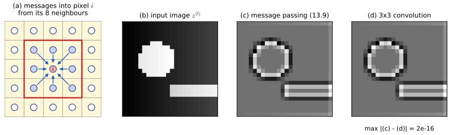
fig_13_3. Reproduces Bishop and Bishop (2024), Figure 13.3, which shows panel (a) as a schematic. Download: PDF · SVG13.2.2 Graph convolutional networks
See also the companion course, Section 8.4.4 (the sum-product algorithm) and Section 8.4.7 (loopy belief propagation): message passing with fixed, probabilistic messages.
pp. 414–415 Every node \(n\) carries a vector \(\bh_n^{(l)}\in\R^D\) in layer \(l\). One layer has two stages: aggregate the neighbours' vectors with a function that does not depend on their order,
\[ \bz_n^{(l)}=\Agg\big(\{\bh_m^{(l)}:m\in\nb(n)\}\big), \tag{13.10} \]then update the node from its own vector and the aggregate,
\[ \bh_n^{(l+1)}=\Upd\big(\bh_n^{(l)},\bz_n^{(l)}\big), \tag{13.11} \]both applied in parallel at every node with the same parameters. Usually \(\bh_n^{(0)}=\bx_n\); layers may have their own parameters or share them. This is the message-passing neural network of Gilmer et al. (2017):
Algorithm 13.1 (simple message-passing neural network) p. 415
- Input: an undirected graph \(\cG=(\cV,\cE)\), initial embeddings \(\bh_n^{(0)}=\bx_n\), functions \(\Agg\) and \(\Upd\).
- For \(l=0,\dots,L-1\): for every node \(n\), \(\bz_n^{(l)}\leftarrow\Agg(\{\bh_m^{(l)}:m\in\nb(n)\})\) and \(\bh_n^{(l+1)}\leftarrow\Upd(\bh_n^{(l)},\bz_n^{(l)})\).
- Return \(\{\bh_n^{(L)}\}\).
Result 13.2 (message passing is equivariant; readouts are invariant) pp. 414, 418–420, (13.19), (13.23); Exercise 13.7
Let \(\Agg\) be a function of a finite multiset (it sees the neighbours' vectors but not their labels) and \(\Upd\) any function, both the same at every node. Write one layer as \(\bH^{(l+1)}=F(\bH^{(l)},\bA)\). Then:
- Each layer is equivariant: \(F(\bP\bH,\bP\bA\bP^\T)=\bP F(\bH,\bA)\) for every permutation matrix \(\bP\).
- A stack of such layers (13.18) is equivariant (Exercise 13.7).
- A readout \(y=f\big(\sum_n\bh_n^{(L)}\big)\) (13.23), or with the mean or element-wise maximum over nodes, is invariant.
Proof
(1) Let \(\widetilde\bH=\bP\bH\), \(\widetilde\bA=\bP\bA\bP^\T\), so \(\tilde\bh_n=\bh_{\pi(n)}\) and \(\tilde A_{nm}=A_{\pi(n)\pi(m)}\) (Result 13.1). The neighbours of \(n\) in the new graph are \[\widetilde\nb(n)=\{m:A_{\pi(n)\pi(m)}=1\}=\pi^{-1}(\nb(\pi(n))).\] Their vectors form the multiset \[ \{\tilde\bh_m:m\in\widetilde\nb(n)\}=\{\bh_{\pi(m)}:\pi(m)\in\nb(\pi(n))\}=\{\bh_k:k\in\nb(\pi(n))\}, \] the same multiset as old node \(\pi(n)\) received. Because \(\Agg\) depends on the multiset only, \(\tilde\bz_n=\bz_{\pi(n)}\), and because \(\Upd\) is the same at every node, \[\tilde\bh_n^{\rm new}=\Upd(\tilde\bh_n,\tilde\bz_n)=\Upd(\bh_{\pi(n)},\bz_{\pi(n)})=\bh^{\rm new}_{\pi(n)},\] which is row \(n\) of \(\bP F(\bH,\bA)\). Both conditions are needed: a node-specific update, or an aggregation that sees labels (as in Filling the gap 13.2), breaks the argument.
(2) By induction on \(l\): \(\bH^{(0)}=\bX\) becomes \(\bP\bX\) by (13.4). If the reordered input to layer \(l\) is \(\bP\bH^{(l-1)}\), then by (1) its output is \(F(\bP\bH^{(l-1)},\bP\bA\bP^\T,\bW^{(l)})=\bP\bH^{(l)}\). Note that the same \(\bP\) acts on the adjacency matrix in every layer, which is (13.19).
(3) \(\sum_n\tilde\bh_n=\sum_n\bh_{\pi(n)}=\sum_k\bh_k\) since \(\pi\) is a bijection; the same reindexing works for the mean and the maximum. ∎
Numerically: over all 120 orders of the graph of Figure 13.2 the equivariance error of a layer is exactly 0 and the sum readout changes by at most \(4\times10^{-16}\) (rounding in a different summation order), Figure 13.S1; for sum, mean, Kipf, GCN, max and attention layers on random graphs the error is below \(3\times10^{-16}\).
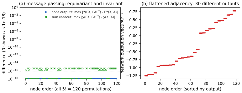
fig_13_s1. Download: PDF · SVG13.2.3 Aggregation operators
pp. 416–417 The aggregation must depend only on the set of incoming vectors, work for any number of them, and be differentiable in its parameters. The simplest choice, from (13.9), is the sum,
\[ \Agg\big(\{\bh_m^{(l)}:m\in\nb(n)\}\big)=\sum_{m\in\nb(n)}\bh_m^{(l)}, \tag{13.12} \]which has no parameters. Nodes with many neighbours then receive large inputs, a problem when degrees range over orders of magnitude (social networks), and the mean avoids it,
\[ \Agg\big(\{\bh_m^{(l)}:m\in\nb(n)\}\big)=\frac1{|\nb(n)|}\sum_{m\in\nb(n)}\bh_m^{(l)}, \tag{13.13} \]at the cost of discarding the degree. Kipf and Welling weight each neighbour by both degrees,
\[ \Agg\big(\{\bh_m^{(l)}:m\in\nb(n)\}\big)=\sum_{m\in\nb(n)}\frac{\bh_m^{(l)}}{\sqrt{|\nb(n)||\nb(m)|}}, \tag{13.14} \]and the element-wise maximum (or minimum) is another valid choice. In matrix form, with \(\bH\) the matrix of rows \(\bh_m^\T\), the first three are \(\bA\bH\), \(\bD^{-1}\bA\bH\) and \(\bD^{-1/2}\bA\bD^{-1/2}\bH\) (Exercise 13.6); the maximum is not linear.
Filling the gap 13.3: in what sense the mean is "provably less powerful" than the sum p. 416
The book cites Hamilton (2020) for this. The statement is about which multisets of neighbour vectors an aggregation can tell apart.
Derivation
See Result 13.3 below for the statements; here is the reasoning. An aggregation is a function of the multiset of neighbour vectors. If it maps two different multisets to the same value, then no update function, however flexible, can treat the two nodes differently. The mean of a multiset depends only on the proportions of its elements: \(\{a\}\), \(\{a,a\}\) and \(\{a,a,a\}\) all have mean \(a\); \(\{a,b\}\) and \(\{a,a,b,b\}\) both have mean \((a+b)/2\). The maximum depends only on the underlying set: \(\{a,b\}\) and \(\{a,a,b\}\) have the same maximum. The sum keeps the counts. With constant input features (no node data, say \(\bh_m^{(0)}=1\)) a mean aggregator therefore cannot even see the degree of a node, while the sum computes it in one layer. Which is preferable depends on the task: when the features matter more than the structure, the mean's insensitivity to degree is a useful normalisation; when counts matter (how many hydrogen atoms are bonded to this carbon?) it is a loss of information. Xu et al. (2019) made this precise by comparing aggregators with the Weisfeiler–Lehman test of Filling the gap 13.7. ∎
Result 13.3 (what sum, mean and max aggregation can distinguish) pp. 416–417
- Mean aggregation maps the multisets \(\{a\}\) and \(\{a,a\}\) (and \(\{a,b\}\), \(\{a,a,b,b\}\)) to the same value; max aggregation maps \(\{a\}\), \(\{a,a\}\) and \(\{a,b\},\{a,a,b\}\) to the same values. Sum aggregation separates all of these.
- (Sum with a feature map can be injective.) Let the node features take values in a finite set \(\{0,1,\dots,K-1\}\) and let multisets have fewer than \(B\) elements. With \(\phi(x)=B^{-x}\), the map \(S\mapsto\sum_{x\in S}\phi(x)\) is injective on such multisets.
Proof
(1) Direct computation (Figure 13.S6(d)).
(2) Let \(c_x\in\{0,\dots,B-1\}\) be the number of copies of \(x\) in \(S\). Then \(\sum_{x\in S}\phi(x)=\sum_{x=0}^{K-1}c_xB^{-x}\) is the number whose base-\(B\) digits are \(c_0.c_1c_2\ldots c_{K-1}\). Base-\(B\) expansions with finitely many digits, each in \(\{0,\dots,B-1\}\), are unique, so the counts, hence the multiset, can be read off the sum. (This is the construction of Xu et al. 2019 and Zaheer et al. 2017 for countable feature sets; a direct computation confirms it for all 34 multisets of at most 4 elements from \(\{0,1,2\}\) with \(B=5\).) ∎
Spectral motivation for (13.14). The book gives (13.14) without motivation. It comes from viewing the layer as a filter in the eigenbasis of a normalised Laplacian, and the same analysis explains the self-loops in the GCN of Kipf and Welling.
Result 13.4 (spectra of the normalised matrices) p. 416, (13.14)
Let \(\cG\) have no isolated nodes, and let \(\bL=\bI-\bD^{-1/2}\bA\bD^{-1/2}\) be its normalised Laplacian. Then
- \[\bx^\T\bL\bx=\sum_{(n,m)\in\cE}\big(x_n/\sqrt{d_n}-x_m/\sqrt{d_m}\big)^2,\] and the eigenvalues of \(\bL\) lie in \([0,2]\).
- The multiplicity of the eigenvalue 0 is the number of connected components; on each component the eigenvector is proportional to \(\sqrt{d_n}\).
- 2 is an eigenvalue if and only if some component is bipartite.
- With self-loops added, \(\Ah=\tD^{-1/2}\tA\tD^{-1/2}\) (\(\tA=\bA+\bI\), \(\tD=\bD+\bI\)) has all eigenvalues in \((-1,1]\); the eigenvalue 1 has eigenvector \(\sqrt{d_n+1}\) on each component. Thus the Kipf–Welling matrix \(\bD^{-1/2}\bA\bD^{-1/2}\) of (13.14) has spectrum in \([-1,1]\), with \(-1\) present exactly for bipartite graphs, while \(\Ah\) never has \(-1\).
Proof
(1) Put \(\by=\bD^{-1/2}\bx\). Then \(\bx^\T\bx=\sum_nd_ny_n^2\) and \[\bx^\T\bD^{-1/2}\bA\bD^{-1/2}\bx=\by^\T\bA\by=\sum_{n,m}A_{nm}y_ny_m.\] Since \(\sum_mA_{nm}=d_n\), \[ \bx^\T\bL\bx=\sum_nd_ny_n^2-\sum_{n,m}A_{nm}y_ny_m=\tfrac12\sum_{n,m}A_{nm}(y_n-y_m)^2=\sum_{(n,m)\in\cE}(y_n-y_m)^2\ge0, \] and in the same way \(\bx^\T(2\bI-\bL)\bx=\sum_{(n,m)\in\cE}(y_n+y_m)^2\ge0\). So \(0\le\bx^\T\bL\bx\le2\bx^\T\bx\), and since \(\bL\) is symmetric its eigenvalues (the values of the Rayleigh quotient at the eigenvectors) lie in \([0,2]\).
(2) \(\bL\bx=\bzero\) iff \(\bx^\T\bL\bx=0\) (for a positive semi-definite matrix, as in Filling the gap 7.2) iff \(y_n=y_m\) on every edge iff \(\by\) is constant on each component. The space of such \(\by\) has dimension equal to the number of components, and \(\bx=\bD^{1/2}\by\).
(3) \(\bL\bx=2\bx\) iff \(y_n=-y_m\) on every edge. On a component, fix \(y\) at one node; then \(y=\pm c\) alternates along every walk, which is consistent iff the component has no odd cycle, i.e. is bipartite, and then \(\by\ne\bzero\) exists.
(4) Apply the same computation to the graph with self-loops, \(\tA\), whose row sums are \(\tilde d_n=d_n+1\). With \(\by=\tD^{-1/2}\bx\), \[ \bx^\T(\bI-\Ah)\bx=\tfrac12\sum_{n,m}\tilde A_{nm}(y_n-y_m)^2\ge0,\qquad \bx^\T(\bI+\Ah)\bx=\tfrac12\sum_{n,m}\tilde A_{nm}(y_n+y_m)^2\ge\tfrac12\sum_n\tilde A_{nn}(2y_n)^2=2\sum_ny_n^2>0 \] for \(\bx\ne\bzero\): the diagonal (self-loop) terms make \(\bI+\Ah\) positive definite, so every eigenvalue of \(\Ah\) exceeds \(-1\). The first identity gives eigenvalues \(\le1\) with equality iff \(\by\) is constant on components, as in (2). ∎
An isolated node (degree 0) is a convention problem for \(\bD^{-1/2}\): with the usual choice \(0^{-1/2}:=0\) it contributes a zero row to \(\bD^{-1/2}\bA\bD^{-1/2}\) and the eigenvalue 1 to \(\bL\). A direct computation confirms (1)–(2) on 150 random graphs with this convention, (3) on a ring of 16 (largest eigenvalue 2) against the karate club (1.715), and (4): the ring's \(\Ah\) has smallest eigenvalue \(-1/3\).
Filling the gap 13.4: from spectral filters to the GCN layer, and why the self-loops p. 416, (13.14), (13.17)
Where does the normalisation \(1/\sqrt{d_nd_m}\) come from, and why do practical GCNs add self-loops?
Derivation
Graph Fourier transform. Write \(\bL=\bU\bm\Lambda\bU^\T\) with orthonormal eigenvectors. By Result 13.4(1), an eigenvector with small eigenvalue varies little across edges (after scaling by \(\sqrt{d_n}\)), one with eigenvalue near 2 flips sign across edges: the eigenvalues play the role of frequencies. A spectral filter multiplies each frequency component by a gain, \(g(\bL)\bx=\bU g(\bm\Lambda)\bU^\T\bx\). Two problems: the eigendecomposition costs \(O(N^3)\), and an arbitrary \(g\) mixes all nodes.
Polynomial filters are local. If \(g(\lambda)=\sum_{k=0}^K\theta_k\lambda^k\), then \(g(\bL)=\sum_k\theta_k\bL^k\) needs no eigenvectors, and \((\bL^k)_{nm}=0\) whenever \(\dist(n,m)>k\) (\(\bL\) has nonzeros only on edges and the diagonal, so this is the walk-counting argument of Section 13.1.2): a degree-\(K\) filter is a \(K\)-hop message-passing operation (Hammond et al. 2011; Defferrard et al. 2016).
First order. Take \(K=1\): \[g(\bL)\bx=\theta_0\bx+\theta_1(\bL-\bI)\bx=\theta_0\bx-\theta_1\bD^{-1/2}\bA\bD^{-1/2}\bx\] (the shift by \(\bI\) centres the spectrum \([0,2]\) at 0). Tying \(\theta=\theta_0=-\theta_1\) leaves one parameter per channel: \[ g(\bL)\bx=\theta\big(\bI+\bD^{-1/2}\bA\bD^{-1/2}\big)\bx, \] whose neighbour part is exactly the Kipf–Welling aggregation (13.14), plus the node itself. With \(D\) input and \(D'\) output channels, \(\theta\) becomes a \(D\times D'\) matrix and we get a layer \(f\big((\bI+\bD^{-1/2}\bA\bD^{-1/2})\bH\bW\big)\).
Why renormalise. \(\bI+\bD^{-1/2}\bA\bD^{-1/2}\) has eigenvalues in \([0,2]\). Stacking \(L\) layers multiplies by its \(L\)th power: components with eigenvalue near 2 are amplified by up to \(2^L\) and, on bipartite graphs, the component with eigenvalue 0 is wiped out. Kipf and Welling (2017) replace it by \(\Ah=\tD^{-1/2}(\bA+\bI)\tD^{-1/2}\), the same construction with the self-loop counted in the degrees. By Result 13.4(4) its spectrum is in \((-1,1]\): repeated application neither explodes nor flips sign forever. This is the matrix behind the GCN layer \(\bH\leftarrow f(\Ah\bH\bW)\) used in the demos, and it is (13.17) (\(\bW_{\rm self}=\bW_{\rm neigh}\), sum over \(\nb(n)\cup\{n\}\)) with symmetric degree weights. The price, analysed in Section 13.3.4, is that \(\Ah^k\) converges, which is over-smoothing. ∎
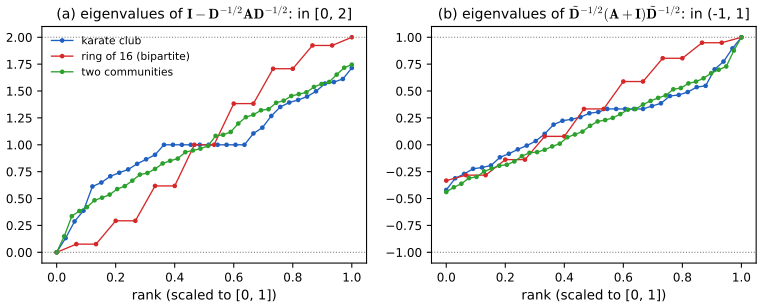
fig_13_s2. Download: PDF · SVGReceptive field. pp. 416–417 Each layer lets information travel one edge, so a node's output in layer \(L\) depends on a growing part of the graph, as the receptive field of a convolutional filter grows with depth (Figure 13.4). Large sparse graphs may need many layers before every output depends on every input; adding a super-node linked to all nodes shortcuts this.
Result 13.5 (the receptive field is the \(L\)-hop neighbourhood) pp. 416–417, Figure 13.4
- For any message-passing network (Algorithm 13.1), \(\bh_n^{(L)}\) is a function of \(\{\bx_m:\dist(n,m)\le L\}\) only.
- For a linear GCN stack \(\bH^{(L)}=\Ah^L\bX\bW\) (or with a strictly increasing activation), the dependence is genuine: \(\partial\bh_n^{(L)}/\partial\bx_m\ne\bzero\) for every \(m\) with \(\dist(n,m)\le L\), for generic weights.
- So every output depends on every input iff \(L\) is at least the diameter. A super-node joined to every node makes the diameter at most 2.
Proof
(1) Induction on \(L\). For \(L=0\), \(\bh_n^{(0)}=\bx_n\). If \(\bh_m^{(L-1)}\) depends only on the ball \(B_{L-1}(m)=\{k:\dist(m,k)\le L-1\}\), then \[\bh_n^{(L)}=\Upd(\bh_n^{(L-1)},\Agg\{\bh_m^{(L-1)}:m\in\nb(n)\})\] depends only on \(\bigcup_{m\in\nb(n)\cup\{n\}}B_{L-1}(m)=B_L(n)\), because a node is within \(L\) of \(n\) iff it is within \(L-1\) of \(n\) or of one of its neighbours.
(2) \((\Ah^L)_{nm}=\sum\Ah_{nk_1}\Ah_{k_1k_2}\cdots\Ah_{k_{L-1}m}\) over walks in the graph with self-loops; all terms are \(\ge0\), and there is a positive one iff some walk of length \(L\) (pauses allowed) joins \(n\) to \(m\), i.e. iff \(\dist(n,m)\le L\). So \(\partial\bh_n^{(L)}/\partial\bx_m=(\Ah^L)_{nm}\bW^\T\ne\bzero\) for \(\bW\ne\bzero\). With a nonlinearity whose derivative is positive (tanh), the chain rule gives a sum over the same walks of products of positive derivatives and weights, which vanishes only on a measure-zero set of weights.
(3) Immediate from (1)–(2); with a super-node \(s\), any two nodes are joined by the walk \(n,s,m\). ∎
A numerical experiment computes the autograd Jacobian of a 3-layer tanh GCN on the karate club: its nonzero pattern is exactly the \(L\)-hop ball for \(L=1,2,3\). The club's diameter is 5; with a super-node it is 2.
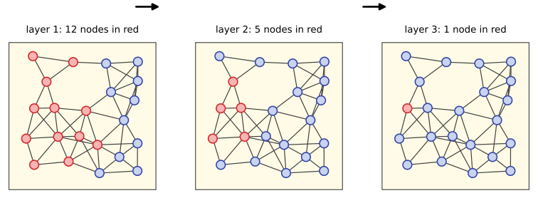
fig_13_4. Reproduces Bishop and Bishop (2024), Figure 13.4. Download: PDF · SVGLearnable aggregation and deep sets. p. 417 Parameters enter the aggregation if each neighbour's vector is first transformed by a shared network and the sum is transformed again:
\[ \Agg\big(\{\bh_m^{(l)}:m\in\nb(n)\}\big)=\MLP_{\bm\theta}\Big(\sum_{m\in\nb(n)}\MLP_{\bm\phi}(\bh_m^{(l)})\Big). \tag{13.15} \]The book states that (13.15) is a universal approximator of permutation-invariant functions of a set (Zaheer et al. 2017), and that the sum may be replaced by a mean, maximum or minimum. For a set without edges the same construction, summing over all other elements, is the deep sets architecture.
Filling the gap 13.5: why sums of learned features can represent every continuous function of a set p. 417, (13.15)
We prove the statement for multisets of \(M\) real numbers, which carries the idea; vector elements need a larger latent dimension (Zaheer et al. 2017; Wagstaff et al. 2019).
Derivation
Claim. Let \(f\) be a continuous, symmetric function of \((x_1,\dots,x_M)\in[a,b]^M\). Then \(f(x_1,\dots,x_M)=\rho\big(\sum_{m}\bm\phi(x_m)\big)\) with \(\bm\phi(x)=(x,x^2,\dots,x^M)\) and \(\rho\) continuous; replacing \(\rho\) and \(\bm\phi\) by networks gives uniform approximations of \(f\) of the form (13.15).
Step 1: the power sums determine the multiset. Let \(p_k=\sum_mx_m^k\), \(k=1,\dots,M\), and let \(e_k\) be the elementary symmetric polynomials (\(e_1=\sum x_m\), \(e_2=\sum_{m<m'}x_mx_{m'}\), ...). Newton's identities \(ke_k=\sum_{i=1}^k(-1)^{i-1}e_{k-i}p_i\) (\(e_0=1\)) compute \(e_1,\dots,e_M\) from \(p_1,\dots,p_M\). The \(e_k\) are, up to sign, the coefficients of \(\prod_m(t-x_m)=\sum_k(-1)^ke_kt^{M-k}\), and a monic polynomial determines its roots with multiplicity. So \(\Phi(x_1,\dots,x_M)=\sum_m\bm\phi(x_m)\) takes the same value on two inputs iff they are permutations of each other. (A numerical experiment recovers 4 random numbers from their 4 power sums this way, to \(10^{-15}\).)
Step 2: \(\rho\) is continuous. Since \(f\) is symmetric, \(\rho(\bm p):=f(\bx)\) for any \(\bx\) with \(\Phi(\bx)=\bm p\) is well defined on the image \(K=\Phi([a,b]^M)\), and \(f=\rho\circ\Phi\). Let \(\bm p_j\to\bm p\) in \(K\) with \(\bm p_j=\Phi(\bx_j)\); sorting each \(\bx_j\) we may take them in the compact set \([a,b]^M\). Any subsequence has a further subsequence \(\bx_j\to\bx^*\) with \(\Phi(\bx^*)=\bm p\) by continuity of \(\Phi\), so \(\rho(\bm p_j)=f(\bx_j)\to f(\bx^*)=\rho(\bm p)\). Every subsequence having a sub-subsequence converging to \(\rho(\bm p)\), the whole sequence does: \(\rho\) is continuous on the compact set \(K\), and by Tietze's theorem it extends to a continuous function on a box containing \(K\).
Step 3: networks. By universal approximation (Section 6.2.2) choose \(\MLP_{\bm\phi}\) within \(\delta/M\) of \(\bm\phi\) on \([a,b]\), so the sums are within \(\delta\) of \(\Phi\); \(\rho\) is uniformly continuous on the box, so for small \(\delta\) the error \(|\rho(\Phi)-\rho(\Phi+\bm\epsilon)|\) is below \(\varepsilon/2\); then choose \(\MLP_{\bm\theta}\) within \(\varepsilon/2\) of \(\rho\) on the box. The composition is within \(\varepsilon\) of \(f\) uniformly.
Remarks. The latent dimension \(M\) grows with the set size, and Wagstaff et al. (2019) show that for continuous \(\bm\phi\) this cannot be avoided in general. With a max instead of a sum the construction fails (Step 1 needs the counts). The book's sentence that deep sets arise from "a graph having no edges" when "the summation is taken over all other vectors" describes message passing on the complete graph: every element receives the aggregate of all others, so a set is a graph in which every pair is linked identically. ∎
13.2.4 Update operators
p. 418 By analogy with (13.9), a simple update is
\[ \Upd\big(\bh_n^{(l)},\bz_n^{(l)}\big)=f\big(\bW_{\rm self}\bh_n^{(l)}+\bW_{\rm neigh}\bz_n^{(l)}+\bb\big), \tag{13.16} \]with an element-wise activation \(f\) and learnable \(\bW_{\rm self},\bW_{\rm neigh},\bb\). With sum aggregation and \(\bW_{\rm self}=\bW_{\rm neigh}\) it becomes
\[ \bh_n^{(l+1)}=f\Big(\bW_{\rm neigh}\sum_{m\in\nb(n)\cup\{n\}}\bh_m^{(l)}+\bb\Big), \tag{13.17} \](the book writes the index set as "\(m\in\nb(n),n\)"). The embeddings may be initialised with \(\bx_n\), padded with zeros or mapped linearly to another dimension, or, without node data, with a one-hot code of the degree. Collecting the embeddings as rows of \(\bH^{(l)}\), a network is a sequence of layers
\[ \bH^{(1)}=F\big(\bX,\bA,\bW^{(1)}\big),\quad \bH^{(2)}=F\big(\bH^{(1)},\bA,\bW^{(2)}\big),\quad\dots,\quad \bH^{(L)}=F\big(\bH^{(L-1)},\bA,\bW^{(L)}\big), \tag{13.18} \]each of which is equivariant,
\[ \bP\bH^{(l)}=F\big(\bP\bH^{(l-1)},\bP\bA\bP^\T,\bW^{(l)}\big), \tag{13.19} \]so the whole network is (Result 13.2, Exercise 13.7).
Filling the gap 13.6: the layer in matrix form, and a dimension slip in Exercise 13.6 p. 426, (13.43)–(13.44)
Matrix form is how the layer is implemented, and the transposes matter.
Derivation
Row \(n\) of \(\bA\bH\) is \(\sum_mA_{nm}\bh_m^\T=\sum_{m\in\nb(n)}\bh_m^\T=\bz_n^\T\) for the sum (13.43), so \(\bZ=\bA\bH\). In (13.16) the vectors are columns and \(\bW_{\rm self}\in\R^{D'\times D}\) multiplies from the left; transposing, row \(n\) of the pre-activation is \(\bh_n^\T\bW_{\rm self}^\T+\bz_n^\T\bW_{\rm neigh}^\T+\bb^\T\). Stacking the rows, \[ \bA\bH\bW_{\rm neigh}^\T+\bH\bW_{\rm self}^\T+\one_N\bb^\T\in\R^{N\times D'}. \] The book's (13.44) reads \(\bA\bH\bW_{\rm neigh}+\bH\bW_{\rm self}+\one_D\bb^\T\). The transposes are a matter of convention (store the weights as \(D\times D'\) matrices acting on rows, as the code here does); but the ones vector must have \(N\) entries, one per node, since \(\one\bb^\T\) must have the shape \(N\times D'\) of the other two terms: \(\one_D\) is a slip for \(\one_N\). With mean or Kipf–Welling aggregation replace \(\bA\) by \(\bD^{-1}\bA\) or \(\bD^{-1/2}\bA\bD^{-1/2}\); (13.17) is \(f\big((\bA+\bI)\bH\bW^\T+\one_N\bb^\T\big)\). The cost of a layer is \(O(|\cE|D'+ND D')\) when \(\bA\) is stored as a sparse matrix (multiply by \(\bW\) first if \(D'<D\)). ∎
Filling the gap 13.7: initialisations that keep equivariance, and what message passing cannot see p. 418
The book lists ways to initialise \(\bh_n^{(0)}\). Which keep the symmetry, and how much can a message-passing network distinguish at all?
Derivation
Initialisations. Zero padding, a shared linear map \(\bh_n^{(0)}=\bW\bx_n\) and a one-hot code of the degree \(d_n\) are all of the form \(\bh_n^{(0)}=g(\bx_n,d_n)\) with the same \(g\) at every node; since reordering sends \((\bx_n,d_n)\) to \((\bx_{\pi(n)},d_{\pi(n)})\), the initial embeddings are equivariant and Result 13.2 applies. A one-hot code of the node's index (\(\bX=\bI\), used for the karate club in the demos and by Kipf and Welling) is different: after reordering the input is \(\bI\) again, not \(\bP\bI\), so the network learns a separate input vector for each labelled position. That is fine transductively (one fixed graph, one fixed numbering) but such a model cannot be applied to a new graph.
A limit: colour refinement. Give every node the same colour and repeat: a node's new colour is the pair (its colour, the multiset of its neighbours' colours), recoded as a new colour. This is the one-dimensional Weisfeiler–Lehman test. Claim: if all nodes start with the same embedding, then for any message-passing network \(\bh_n^{(l)}\) is a function of the colour of \(n\) after \(l\) rounds. Induction: if \(\bh_m^{(l-1)}=g_{l-1}(c_m^{(l-1)})\) for all \(m\), then \[\bh_n^{(l)}=\Upd(g_{l-1}(c_n^{(l-1)}),\Agg\{g_{l-1}(c_m^{(l-1)})\})\] is a function of the pair \((c_n^{(l-1)},\{c_m^{(l-1)}:m\in\nb(n)\})\), i.e. of \(c_n^{(l)}\). Hence if two graphs have the same multiset of colours in every round, every message-passing network with an invariant readout gives them the same output (Xu et al. 2019; Morris et al. 2019). Two triangles and one hexagon are both 2-regular: every node sees two neighbours of its own colour in every round, so no network of this chapter can tell them apart, although one graph is connected and the other is not (Figure 13.S6). Sum aggregation with injective updates attains this limit (Result 13.3(2)); mean and max fall short of it. ∎
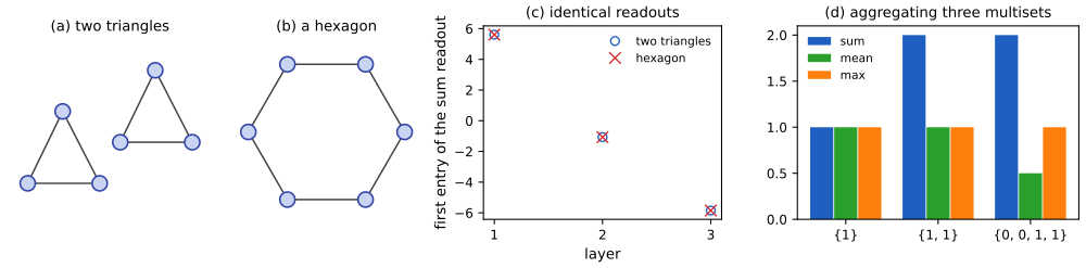
fig_13_s6. Download: PDF · SVG13.2.5 Node classification
See also the companion course, Section 4.3.4 (softmax and cross-entropy); in this course, Section 5.4.4 and Section 6.4.3.
pp. 419–420 After the last message-passing layer a readout layer turns each node's embedding into class probabilities with a softmax shared by all nodes,
\[ y_{ni}=\frac{\exp(\bw_i^\T\bh_n^{(L)})}{\sum_j\exp(\bw_j^\T\bh_n^{(L)})}, \tag{13.20} \]\(i=1,\dots,C\), and training minimises the cross-entropy over the labelled nodes \(\cV_{\rm train}\), with one-hot targets \(t_{ni}\),
\[ \cL=-\sum_{n\in\cV_{\rm train}}\sum_{i=1}^Ct_{ni}\ln y_{ni}. \tag{13.21} \]Erratum. The book prints (13.21) as \(-\sum_n\sum_iy_{ni}^{t_{ni}}\), without the logarithm. The cross-entropy is \(-\sum t_{ni}\ln y_{ni}=-\ln\prod_ny_{n,c(n)}\) (minus the log-likelihood of the labels, Section 6.4.3); the printed expression equals \(-\sum_n\big(y_{n,c(n)}+C-1\big)\), which rewards the sum of the true-class probabilities instead of their product and is not a log-likelihood (for true-class probabilities 0.9, 0.6, 0.3 and \(C=2\): 1.820 against \(-4.8\); checked).
Because the weights are shared the outputs are equivariant and the loss is invariant (reordering nodes, data and the set \(\cV_{\rm train}\) together leaves \(\cL\) unchanged; checked to \(10^{-12}\)). For a continuous target use a linear readout and a sum-of-squares error. The book distinguishes three kinds of nodes: training nodes \(\cV_{\rm train}\), labelled, in the loss and in message passing; transductive nodes \(\cV_{\rm trans}\), unlabelled, not in the loss but passing messages during training and inference, and labelled at the end; inductive nodes \(\cV_{\rm induct}\), which together with their edges take part only at inference. Without transductive nodes the setting is inductive (supervised) learning; with them it is transductive, a form of semi-supervised learning.
Filling the gap 13.8: the gradients of a GCN node classifier, in matrix form pp. 419–420, (13.20)–(13.21)
The book leaves gradients to automatic differentiation. Writing them out shows how a loss on a few labelled nodes reaches the parameters through the graph; they are the gradients that the live demo computes by hand.
Derivation
The network. For \(l=0,\dots,L-1\): \(\bS_l=\Ah\bH_l\), \(\bZ_l=\bS_l\bW_l+\one_N\bb_l^\T\), and \(\bH_{l+1}=\tanh(\bZ_l)\) for \(l<L-1\) (plus \(\bH_l\) with a residual connection), with \(\bH_0=\bX\). The last \(\bZ_{L-1}\) holds the logits; \(\bY=\softmax(\bZ_{L-1})\) row by row. The loss is the mean of (13.21) over the \(n_{\rm tr}=|\cV_{\rm train}|\) labelled nodes plus weight decay, \[\cL=-\frac1{n_{\rm tr}}\sum_{n\in\cV_{\rm train}}\sum_it_{ni}\ln y_{ni}+\frac\lambda2\sum_l\|\bW_l\|_F^2.\] Let \(\bM=\diag(m_n)\) with \(m_n=1\) on labelled nodes and 0 elsewhere.
Output layer. For one node, \(\partial(-\sum_it_i\ln y_i)/\partial z_j=y_j-t_j\) (the softmax–cross-entropy derivative, Section 5.4.4). So \(\bG_{L-1}:=\partial\cL/\partial\bZ_{L-1}=\bM(\bY-\bT)/n_{\rm tr}\): only labelled rows are nonzero.
One layer back. Use differentials: \(\d\cL=\Tr(\bG_l^\T\d\bZ_l)\) with \(\d\bZ_l=\d\bS_l\,\bW_l+\bS_l\,\d\bW_l+\one\,\d\bb_l^\T\) and \(\d\bS_l=\Ah\,\d\bH_l\). With \(\Tr(\bm A^\T\bm B\bm C)=\Tr((\bm B^\T\bm A)^\T\bm C)\), \[ \frac{\partial\cL}{\partial\bW_l}=\bS_l^\T\bG_l+\lambda\bW_l,\qquad \frac{\partial\cL}{\partial\bb_l}=\bG_l^\T\one_N,\qquad \frac{\partial\cL}{\partial\bH_l}=\Ah^\T\bG_l\bW_l^\T. \] Through \(\bH_l=\tanh(\bZ_{l-1})\) (element-wise, \(\tanh'=1-\tanh^2\)): \(\bG_{l-1}=\frac{\partial\cL}{\partial\bH_l}\odot(1-\bH_l^{\odot2})\). With a residual connection \(\bH_l=\tanh(\bZ_{l-1})+\bH_{l-1}\), the same \(\partial\cL/\partial\bH_l\) is also added to \(\partial\cL/\partial\bH_{l-1}\).
How the unlabelled nodes learn. \(\bG_{L-1}\) has nonzero rows only at labelled nodes, but each step back multiplies by \(\Ah^\T\), which spreads the rows one hop: \(\partial\cL/\partial\bH_l\) is nonzero on the \((L-1-l)\)-hop neighbourhood of the labelled nodes. Their representations, and the weights acting on them, are shaped by the labels. If the edges are removed (\(\Ah=\bI\)) and the features are one-hot (\(\bX=\bI\)), the gradient of the first-layer weight row of an unlabelled node \(m\) is \((\bS_0^\T\bG_0)_{m\cdot}=(\bG_0)_{m\cdot}=\bzero\) plus weight decay: that row only shrinks, and the node's prediction is driven by its random initial row, so the unlabelled nodes are at chance (16 of 32 in Figure 13.S4).
Check. These formulas agree with central differences (\(7\times10^{-11}\), with and without residual connections) and with PyTorch's autograd and cross_entropy (\(10^{-12}\)). ∎
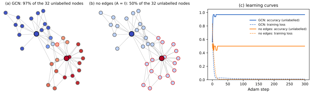
fig_13_s4. Download: PDF · SVGFilling the gap 13.9: transductive and inductive nodes in matrix terms pp. 419–420
The three kinds of nodes are defined in words. In matrices they differ in which rows enter the loss and which rows and columns enter \(\bA\).
Derivation
Order the nodes as training, transductive, inductive. During training, the network runs on the subgraph induced by \(\cV_{\rm train}\cup\cV_{\rm trans}\): its adjacency matrix is the top-left block \(\bA_{\rm tt}\) of \(\bA\), and the loss mask \(\bM\) selects the training rows. At inference the full \(\bA\) is used. Two consequences follow. First, transductive nodes influence the trained weights (through the \(\Ah^\T\) factors of Filling the gap 13.8) although they have no labels; inductive nodes do not. Second, any normalisation that depends on degrees changes between training and inference: a training node with an inductive neighbour has degree \(d_n\) in training and \(d_n+1\) later, so its row of \(\Ah\) changes even though nothing about the node did. Equivariance is unaffected (it holds for every graph), but this train/test mismatch is one reason why inductive methods often prefer mean aggregation, whose weights \(1/|\nb(n)|\) involve only the receiving node, and why the parameters must not depend on \(N\): a message-passing network's parameters do not, so it can be applied to the larger graph. ∎
13.2.6 Edge classification
p. 420 For edge completion, the probability that nodes \(n\) and \(m\) are linked can be modelled from their final embeddings by
\[ p(n,m)=\sigma\big(\bh_n^\T\bh_m\big). \tag{13.22} \]Filling the gap 13.10: the edge model is equivariant, and how it is trained p. 420, (13.22)
Derivation
Symmetry. The matrix of probabilities is \(\bm\Sigma=\sigma(\bH\bH^\T)\) (element-wise), symmetric as an undirected edge model should be. Under reordering \(\bH\to\bP\bH\) it becomes \(\sigma(\bP\bH\bH^\T\bP^\T)=\bP\bm\Sigma\bP^\T\): it transforms like an adjacency matrix, the natural equivariance for pair-level outputs (checked).
Training. With observed pairs \(a_{nm}\in\{0,1\}\) (known edges, and known or sampled non-edges, since there are \(O(N^2)\) non-edges and they are usually subsampled, "negative sampling"), the log-likelihood is a sum of logistic terms \(a\ln\sigma(s)+(1-a)\ln(1-\sigma(s))\) with \(s=\bh_n^\T\bh_m\), exactly logistic regression on the score \(s\) (Section 5.4.3). Its derivative is \((a-\sigma(s))\,\partial s/\partial\bh_n=(a-\sigma(s))\bh_m\): linked pairs pull their embeddings together, sampled non-links push them apart. Since \(s\) is unchanged by \(\bh\to\bm Q\bh\) for any orthogonal \(\bm Q\), the embeddings are identified only up to rotation, which is harmless for prediction. ∎
13.2.7 Graph classification
p. 420 To predict a property of a whole graph from a training set of labelled graphs \(\cG_1,\dots,\cG_N\), combine the final node embeddings in an order-independent way, for example
\[ \by=f\Big(\sum_{n\in\cV}\bh_n^{(L)}\Big), \tag{13.23} \]with \(f\) a learnable map; the mean, maximum or minimum also work. Cross-entropy is used for classification (toxic or safe), squared error for regression (solubility). Graph prediction is always inductive: training and test graphs are different.
Result 13.6 (pair-level and graph-level outputs) p. 420, (13.22)–(13.23)
- The matrix of edge probabilities \(\bm\Sigma=\sigma(\bH\bH^\T)\) of (13.22) is symmetric and reorders like an adjacency matrix: \(\bm\Sigma(\bP\bH)=\bP\bm\Sigma(\bH)\bP^\T\).
- Sum, mean and max readouts (13.23) of an equivariant network are invariant.
- The sum readout can see the size of a graph and the mean cannot: with constant node features \(\bh_n^{(0)}=1\) and one sum-aggregation layer \(h_n=d_n\), the sum readout is \(2|\cE|\), and a mean readout of \(h_n=1+d_n\) gives \(1+2|\cE|/N\), so a graph and two disjoint copies of it get the same mean readout but different sums.
Proof
(1) \(\sigma\) acts element-wise and \((\bP\bH)(\bP\bH)^\T=\bP\bH\bH^\T\bP^\T\); a permutation of rows and columns commutes with an element-wise function. (2) This is Result 13.2(3). (3) \(\sum_nd_n=2|\cE|\) (each edge is counted at both ends). Two disjoint copies double \(N\), \(|\cE|\) and every sum, while every mean is unchanged: in fact every node of the double graph has the same embedding as its counterpart in every layer (message passing is local), so a mean or max readout of any message-passing network cannot separate a graph from two copies of itself, and a sum readout separates them whenever the summed embedding is nonzero. ∎
13.3 General Graph Networks
p. 420 The rest of the chapter outlines extensions of message passing and some practical issues.
13.3.1 Graph attention networks
p. 421 Attention (Section 12.1 of the book) can serve as the aggregation: incoming messages are weighted by coefficients \(A_{nm}\),
\[ \bz_n^{(l)}=\Agg\big(\{\bh_m^{(l)}:m\in\nb(n)\}\big)=\sum_{m\in\nb(n)}A_{nm}\bh_m^{(l)}, \tag{13.24} \]with
\[ A_{nm}\ge0, \tag{13.25} \] \[ \sum_{m\in\nb(n)}A_{nm}=1. \tag{13.26} \]This is a graph attention network (Veličković et al. 2018): some neighbours can matter more than others, depending on the data. The coefficients come from a softmax, for instance of a bilinear score,
\[ A_{nm}=\frac{\exp\big(\bh_n^\T\bW\bh_m\big)}{\sum_{m'\in\nb(n)}\exp\big(\bh_n^\T\bW\bh_{m'}\big)}, \tag{13.27} \]with a learnable \(D\times D\) matrix \(\bW\), or of a network that scores the pair,
\[ A_{nm}=\frac{\exp\{\MLP(\bh_n,\bh_m)\}}{\sum_{m'\in\nb(n)}\exp\{\MLP(\bh_n,\bh_{m'})\}}, \tag{13.28} \]which the book asks to be unchanged when its two inputs are exchanged. With \(H\) heads, each with its own parameters, the head outputs are concatenated and projected linearly; on a fully connected graph, says the book, a multi-head graph attention network "becomes a standard transformer encoder".
Result 13.7 (graph attention is equivariant; on a complete graph with self-loops it is self-attention) p. 421, (13.24)–(13.28); Exercises 13.8, 13.9
- With (13.27), or (13.28) with any shared MLP, the attention matrix reorders as \(\bP\bm{\mathcal A}\bP^\T\) and the aggregation (13.24) is equivariant. The symmetry of the MLP is not needed for this.
- Let every node be linked to every node including itself, and let the messages be \(\bW_v^\T\bh_m\). With \(\bW=\bW_q\bW_k^\T/\sqrt{d_k}\), (13.24) with (13.27) is single-head self-attention \(\softmax(\bQ\bK^\T/\sqrt{d_k})\bm V\), \(\bQ=\bH\bW_q\), \(\bK=\bH\bW_k\), \(\bm V=\bH\bW_v\); \(H\) heads give multi-head attention.
Proof
(1) The score of a pair, \(s(\bh_n,\bh_m)\), depends on the two vectors only. After reordering, new nodes \(n,m\) carry \(\bh_{\pi(n)},\bh_{\pi(m)}\) and are linked iff \(\pi(n),\pi(m)\) were, so \(\tilde A_{nm}=A_{\pi(n)\pi(m)}\): numerator and the normalising sum over \(\widetilde\nb(n)=\pi^{-1}(\nb(\pi(n)))\) are the old ones. Then \(\tilde\bz_n=\sum_m\tilde A_{nm}\tilde\bh_m=\sum_kA_{\pi(n)k}\bh_k=\bz_{\pi(n)}\). Nowhere was \(s(\bh_n,\bh_m)=s(\bh_m,\bh_n)\) used: attention from \(n\) to \(m\) may differ from attention from \(m\) to \(n\) (the softmax normalises over different neighbourhoods anyway, so \(\bm{\mathcal A}\) is not symmetric even for a symmetric score). A direct computation confirms equivariance for a deliberately asymmetric MLP score. A symmetric score is a modelling choice, not a requirement.
(2) On the complete graph with self-loops \(\nb(n)=\{1,\dots,N\}\), so (13.27) is the softmax over all \(m\) of \(\bh_n^\T\bW_q\bW_k^\T\bh_m/\sqrt{d_k}=\bm q_n^\T\bm k_m/\sqrt{d_k}\), the attention weights of a transformer (Section 12.1 of the book), and \(\sum_mA_{nm}\bW_v^\T\bh_m\) is its output (checked to \(10^{-15}\)). The bilinear form with a full \(\bW\) is slightly more general (rank up to \(D\) instead of \(d_k\)). Several heads with concatenation and projection are multi-head attention. ∎
Qualification. The book's statement (and Exercise 13.9) needs three provisos. (i) Self-loops: the chapter's graphs are simple, so \(n\notin\nb(n)\), while a transformer token attends to itself; on a complete simple graph the two differ (checked). (ii) A transformer layer is more than the attention step: value and output projections, a residual connection, layer normalisation and a position-wise MLP; with message passing these are the update (13.16), so "a GAT layer with those components" is a transformer layer. (iii) A transformer adds positional encodings to the tokens; without them it is permutation equivariant like any graph network, and with them it is a graph network whose node features include the position. Conversely, a transformer is a graph network on the complete graph.
13.3.2 Edge embeddings
pp. 421–422 Edges can carry data (bond types) and, even without data, hidden embeddings \(\be_{nm}^{(l)}\) that the network updates:
\[ \be_{nm}^{(l+1)}=\Upd_{\rm edge}\big(\be_{nm}^{(l)},\bh_n^{(l)},\bh_m^{(l)}\big), \tag{13.29} \] \[ \bz_n^{(l+1)}=\Agg_{\rm node}\big(\{\be_{nm}^{(l+1)}:m\in\nb(n)\}\big), \tag{13.30} \] \[ \bh_n^{(l+1)}=\Upd_{\rm node}\big(\bh_n^{(l)},\bz_n^{(l+1)}\big). \tag{13.31} \]The final \(\be_{nm}^{(L)}\) can be used for edge predictions.
13.3.3 Graph embeddings
p. 422 A graph-level embedding \(\bg^{(l)}\) can be kept as well, giving the general message-passing equations of Battaglia et al. (2018):
\[ \be_{nm}^{(l+1)}=\Upd_{\rm edge}\big(\be_{nm}^{(l)},\bh_n^{(l)},\bh_m^{(l)},\bg^{(l)}\big), \tag{13.32} \] \[ \bz_n^{(l+1)}=\Agg_{\rm node}\big(\{\be_{nm}^{(l+1)}:m\in\nb(n)\}\big), \tag{13.33} \] \[ \bh_n^{(l+1)}=\Upd_{\rm node}\big(\bh_n^{(l)},\bz_n^{(l+1)},\bg^{(l)}\big), \tag{13.34} \] \[ \bg^{(l+1)}=\Upd_{\rm graph}\big(\bg^{(l)},\{\bh_n^{(l+1)}:n\in\cV\},\{\be_{nm}^{(l+1)}:(n,m)\in\cE\}\big). \tag{13.35} \]Edges are updated from their old state, their two end nodes and the graph; each node aggregates its edges and updates; the graph updates from all nodes and edges (Figure 13.5 of the book, a schematic not reproduced here, and Algorithm 13.2).
Algorithm 13.2 (graph network with node, edge and graph embeddings) p. 424
- Input: \(\cG=(\cV,\cE)\), initial \(\{\bh_n^{(0)}\}\), \(\{\be_{nm}^{(0)}\}\), \(\bg^{(0)}\).
- For \(l=0,\dots,L-1\): update every edge by (13.32); aggregate at every node by (13.33); update every node by (13.34); update the graph by (13.35).
- Return \(\{\bh_n^{(L)}\}\), \(\{\be_{nm}^{(L)}\}\), \(\bg^{(L)}\).
Result 13.8 (the general graph network is equivariant) p. 422, (13.29)–(13.35)
Store the edge embeddings in an array \(\bm{\mathcal E}\) with entries \(\be_{nm}\) (zero where there is no edge). If each update function is shared (the same for all edges, all nodes), \(\Agg_{\rm node}\) is a multiset function and \(\Upd_{\rm graph}\) depends on the multisets of node and edge embeddings only, then under a reordering \(\pi\): \(\tilde\be_{nm}^{(l)}=\be_{\pi(n)\pi(m)}^{(l)}\) (edges reorder like \(\bP\bA\bP^\T\)), \(\widetilde\bH^{(l)}=\bP\bH^{(l)}\), and \(\tilde\bg^{(l)}=\bg^{(l)}\), for every \(l\).
Proof
Induction on \(l\); at \(l=0\) it is the definition of reordering. Suppose it holds at \(l\). (13.32): \[\tilde\be_{nm}^{(l+1)}=\Upd_{\rm edge}(\be^{(l)}_{\pi(n)\pi(m)},\bh^{(l)}_{\pi(n)},\bh^{(l)}_{\pi(m)},\bg^{(l)})=\be^{(l+1)}_{\pi(n)\pi(m)},\] and the reordered graph has edge \((n,m)\) iff the old one has \((\pi(n),\pi(m))\). (13.33): the multiset \[\{\tilde\be_{nm}^{(l+1)}:m\in\widetilde\nb(n)\}=\{\be_{\pi(n)k}^{(l+1)}:k\in\nb(\pi(n))\},\] so \(\tilde\bz_n=\bz_{\pi(n)}\). (13.34): then \(\tilde\bh_n^{(l+1)}=\bh_{\pi(n)}^{(l+1)}\). (13.35): the multisets of all node and all edge embeddings are unchanged by relabelling, so \(\tilde\bg^{(l+1)}=\bg^{(l+1)}\). A numerical experiment runs one layer with random MLPs on a 6-node graph: all three statements hold to \(10^{-15}\). ∎
13.3.4 Over-smoothing
pp. 422–423 In many graph networks the node embeddings become more and more alike as layers are added, which limits the useful depth: over-smoothing. Two remedies are suggested. Residual connections (Section 9.5 of the book),
\[ \bh_n^{(l+1)}=\Upd_{\rm node}\big(\bh_n^{(l)},\bz_n^{(l+1)},\bg^{(l)}\big)+\bh_n^{(l)}, \tag{13.36} \]and an output layer that sees every layer, e.g. through concatenation (\(\oplus\)),
\[ \by_n=f\big(\bh_n^{(1)}\oplus\bh_n^{(2)}\oplus\dots\oplus\bh_n^{(L)}\big), \tag{13.37} \]or an element-wise max over the layers ("jumping knowledge", Xu et al. 2018). The book does not say why embeddings become alike. For GCN-type layers the reason is spectral, and it can be proved.
Result 13.9 (repeated normalised averaging converges to the leading eigenvector) p. 422, Section 13.3.4
Let \(\cG\) be connected, \(\Ah=\tD^{-1/2}(\bA+\bI)\tD^{-1/2}\) with eigenvalues \(1=\lambda_1>\lambda_2\ge\dots\ge\lambda_N>-1\), and \(\rho=\max(|\lambda_2|,|\lambda_N|)<1\). Let \(\bu\) be the unit vector with \(u_n\propto\sqrt{d_n+1}\). Then for every \(\bX\) and \(k\ge0\)
\[ \big\|\Ah^k\bX-\bu\bu^\T\bX\big\|_F\le\rho^k\big\|\bX-\bu\bu^\T\bX\big\|_F . \]So \(\Ah^k\bX\to\bu\bu^\T\bX\), whose row \(n\) is \(\sqrt{d_n+1}\) times one common vector: apart from its degree, a node's identity is lost. For the mean with self-loops, \((\tD^{-1}\tA)^k\bX\to\one_N\bm\pi^\T\bX\) with \(\pi_n\propto d_n+1\): every node ends at the same point.
Proof
By Result 13.4(4) the eigenvalues lie in \((-1,1]\), and 1 is simple with eigenvector \(\bu\) because the graph is connected (part 2 of that result for the graph with self-loops). So \(\rho<1\). Expand \(\Ah=\sum_i\lambda_i\bu_i\bu_i^\T\) with \(\bu_1=\bu\); then \(\Ah^k=\bu\bu^\T+\sum_{i\ge2}\lambda_i^k\bu_i\bu_i^\T\) and \(\Ah^k\bX-\bu\bu^\T\bX=\sum_{i\ge2}\lambda_i^k\bu_i(\bu_i^\T\bX)\). The rows \(\bu_i^\T\bX\) are the coordinates of the columns of \(\bX\) in the orthonormal basis, so by Pythagoras \[ \|\Ah^k\bX-\bu\bu^\T\bX\|_F^2=\sum_{i\ge2}\lambda_i^{2k}\|\bu_i^\T\bX\|^2\le\rho^{2k}\sum_{i\ge2}\|\bu_i^\T\bX\|^2=\rho^{2k}\|\bX-\bu\bu^\T\bX\|_F^2. \] For the mean, \(\tD^{-1}\tA=\tD^{-1/2}\Ah\tD^{1/2}\), so \[(\tD^{-1}\tA)^k=\tD^{-1/2}\Ah^k\tD^{1/2}\to\tD^{-1/2}\bu\bu^\T\tD^{1/2}.\] With \(u_n=\sqrt{\tilde d_n}/s\), \(s^2=\sum\tilde d_n\), the limit has entries \(\tilde d_m/s^2=\pi_m\) in every row. ∎
On the karate club \(\rho=0.896\) and after 64 propagations the distance to the limit is \(6.3\times10^{-4}\) of the initial one, below the bound \(\rho^{64}=9.0\times10^{-4}\) (Figure 13.S3; checked for every \(k\le64\)). Without self-loops the same argument applies to \(\bD^{-1/2}\bA\bD^{-1/2}\), except on bipartite graphs, where the eigenvalue \(-1\) makes \(\rho=1\): the iteration then oscillates forever (a ring of 16 nodes in the demo), another reason for the self-loops of Filling the gap 13.4.
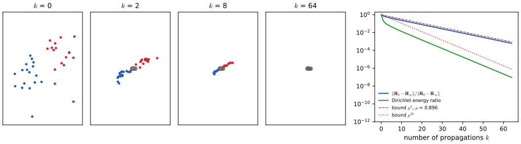
fig_13_s3. Download: PDF · SVGReal layers also multiply by weights and apply a nonlinearity. A convenient measure of how alike the embeddings are is the Dirichlet energy \[E(\bH)=\Tr\big(\bH^\T(\bI-\Ah)\bH\big)=\tfrac12\sum_{n,m}\tilde A_{nm}\big\|\bh_n/\sqrt{\tilde d_n}-\bh_m/\sqrt{\tilde d_m}\big\|^2,\] which is zero exactly on the limit subspace of Result 13.9.
Result 13.10 (GCN layers with ReLU shrink the Dirichlet energy) p. 422, Section 13.3.4
With \(\rho\) as in Result 13.9 and \(\|\bW\|_2\) the largest singular value of \(\bW\):
- \(E(\Ah\bH)\le\rho^2E(\bH)\);
- \(E(\bH\bW)\le\|\bW\|_2^2E(\bH)\);
- \(E(\ReLU(\bH))\le E(\bH)\);
- hence a layer without bias, \(\bH\leftarrow\ReLU(\Ah\bH\bW_l)\), satisfies \(E(\bH^{(l+1)})\le\rho^2\|\bW_l\|_2^2E(\bH^{(l)})\), and if \(\rho\|\bW_l\|_2\le s<1\) for every layer the energy decays at least like \(s^{2l}\).
Proof
(1) In the eigenbasis, \(E(\bH)=\sum_i(1-\lambda_i)\|\bu_i^\T\bH\|^2\) and \(E(\Ah\bH)=\sum_i(1-\lambda_i)\lambda_i^2\|\bu_i^\T\bH\|^2\). The \(i=1\) terms vanish (\(1-\lambda_1=0\)), every other weight \(1-\lambda_i\) is positive, and \(\lambda_i^2\le\rho^2\) for \(i\ge2\).
(2) Each term of the edge form is \[\|\bW^\T(\bh_n/\sqrt{\tilde d_n}-\bh_m/\sqrt{\tilde d_m})\|^2\le\|\bW\|_2^2\|\bh_n/\sqrt{\tilde d_n}-\bh_m/\sqrt{\tilde d_m}\|^2.\]
(3) For \(c>0\), \(\ReLU(a)/c=\ReLU(a/c)\) (positive homogeneity), and \(|\ReLU(a)-\ReLU(b)|\le|a-b|\). So component-wise \[|\ReLU(h_{nj})/\sqrt{\tilde d_n}-\ReLU(h_{mj})/\sqrt{\tilde d_m}|=|\ReLU(h_{nj}/\sqrt{\tilde d_n})-\ReLU(h_{mj}/\sqrt{\tilde d_m})|\le|h_{nj}/\sqrt{\tilde d_n}-h_{mj}/\sqrt{\tilde d_m}|,\] and summing the squares gives the claim.
(4) Combine (3), (2) and (1). ∎
This is the argument of Cai and Wang (2020) (see also Oono and Suzuki 2020). It explains over-smoothing when weights are small; trained weights can be large enough to counteract it, so it is a tendency, not a law. The proof uses positive homogeneity, so it does not cover tanh or biases as stated. All four inequalities hold in 50 random cases.
Result 13.11 (what residual connections do to linear propagation) p. 422, (13.36)–(13.37)
- The linear part of (13.36), \(\bH\leftarrow\bH+\Ah\bH\), rescaled by \(\tfrac12\), is propagation by \(\tfrac12(\bI+\Ah)\), with eigenvalues \(\tfrac12(1+\lambda_i)\in(0,1]\). It converges to the same limit \(\bu\bu^\T\bX\), at rate \(\tfrac12(1+\lambda_2)\ge\lambda_2\): slower when \(\rho=\lambda_2\), but it does not prevent the collapse.
- An initial residual, \(\bH\leftarrow(1-\alpha)\Ah\bH+\alpha\bX\) with \(0<\alpha\le1\), converges at rate \(1-\alpha\) to \[\bH^*=\alpha\big(\bI-(1-\alpha)\Ah\big)^{-1}\bX=\alpha\sum_{k\ge0}(1-\alpha)^k\Ah^k\bX,\] whose component along every eigenvector \(\bu_i\) is \(\alpha/(1-(1-\alpha)\lambda_i)\ne0\) times that of \(\bX\): nothing is lost.
- With concatenation (13.37) the output layer receives \(\bh_n^{(1)}\) unchanged, so whatever the deep layers do, the information of the shallow layers is available to it by construction.
Proof
(1) \(\tfrac12(\bI+\Ah)\) has the eigenvectors of \(\Ah\) and eigenvalues \(\tfrac12(1+\lambda_i)\), all positive since \(\lambda_i>-1\), the largest 1 (simple). Apply the proof of Result 13.9 with the second-largest modulus \(\tfrac12(1+\lambda_2)\). Since \(\lambda_2\le1\), \(\tfrac12(1+\lambda_2)\ge\lambda_2\). On the karate club the rate goes from 0.896 to 0.948 (checked).
(2) The error \(\bm\Delta_k=\bH_k-\bH^*\) obeys \(\bm\Delta_{k+1}=(1-\alpha)\Ah\bm\Delta_k\) because \(\bH^*=(1-\alpha)\Ah\bH^*+\alpha\bX\); since \(\|\Ah\|_2=1\), \(\|\bm\Delta_k\|_F\le(1-\alpha)^k\|\bm\Delta_0\|_F\). The series is the Neumann series of the inverse, which converges for the same reason, and in the eigenbasis the inverse multiplies component \(i\) by \(\alpha/(1-(1-\alpha)\lambda_i)\), positive. With \(\alpha=0.2\) on the karate club the limit keeps 11% of the initial Dirichlet energy (checked). This is the propagation of Gasteiger (Klicpera) et al. (2019).
(3) Immediate. ∎
So in the linear picture (13.36) only slows smoothing down; what makes deep residual networks trainable is that the identity path carries the representation and the gradient past the averaging, and the learned updates can then add what is needed. Figure 13.S5 shows the effect on a trained network.
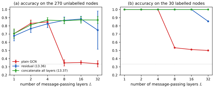
fig_13_s5 (results cached). Download: PDF · SVG13.3.5 Regularization
p. 423 The usual regularisers (penalties such as the sum of squared weights, Chapter 9 of the book) apply. Weights can also be shared across layers, so that (13.18) applies one layer repeatedly. Dropout for graphs omits random nodes in each forward pass, or random entries of the adjacency matrix (edges).
Filling the gap 13.11: dropping edges with rescaling keeps the sum aggregation unbiased p. 423
Derivation
Keep each edge independently with probability \(1-p\), mask \(\xi_{nm}\sim\mathrm{Bernoulli}(1-p)\), and aggregate \(\bz_n=\frac1{1-p}\sum_mA_{nm}\xi_{nm}\bh_m\). Then \[\E[\bz_n]=\frac1{1-p}\sum_mA_{nm}(1-p)\bh_m=\sum_mA_{nm}\bh_m:\] unbiased, as for ordinary dropout, with variance \(\frac{p}{1-p}\sum_mA_{nm}\|\bh_m\|^2\) per node that the network learns to tolerate (checked by Monte Carlo on the karate club). Dropping edges also reduces the effective connectivity in each pass, which slows over-smoothing during training (Rong et al. 2020). For normalised aggregations the rescaling is only approximately unbiased, because the degrees in the normaliser change with the mask. Sharing weights across layers turns the network into a recurrent update \(\bH\leftarrow F(\bH,\bA,\bW)\), the form of classical iterative schemes on graphs such as loopy belief propagation (companion course, Section 8.4.7). ∎
13.3.6 Geometric deep learning
pp. 424–425 Permutation symmetry is an inductive bias that reduces the data needed. Data in space (meshes, fluids, molecules) have more symmetry: a molecule's properties do not change if it is rotated, translated or reflected. Give atom \(n\) a coordinate embedding \(\br_n^{(l)}\in\R^3\), initialised with its position, and update (Satorras, Hoogeboom and Welling 2021)
\[ \be_{nm}^{(l+1)}=\Upd_{\rm edge}\big(\be_{nm}^{(l)},\bh_n^{(l)},\bh_m^{(l)},\|\br_n^{(l)}-\br_m^{(l)}\|^2\big), \tag{13.38} \] \[ \br_n^{(l+1)}=\br_n^{(l)}+C\sum_{(n,m)\in\cE}\big(\br_n^{(l)}-\br_m^{(l)}\big)\phi\big(\be_{nm}^{(l+1)}\big), \tag{13.39} \] \[ \bz_n^{(l+1)}=\Agg_{\rm node}\big(\{\be_{nm}^{(l+1)}:m\in\nb(n)\}\big), \tag{13.40} \] \[ \bh_n^{(l+1)}=\Upd_{\rm node}\big(\bh_n^{(l)},\bz_n^{(l+1)}\big), \tag{13.41} \]with \(\phi\) a scalar network and \(C\) usually one over the number of terms. Squared distances do not change under the transformations, and the coordinates move along relative positions.
Result 13.12 (the layer (13.38)–(13.41) is E(n)-equivariant) pp. 424–425; Exercise 13.10
Let \(\tilde\br_n=\bR\br_n+\bc\) for all \(n\), with \(\bR\) orthogonal (\(\bR\bR^\T=\bR^\T\bR=\bI\), (13.47): rotations and reflections) and \(\bc\) a translation, (13.45)–(13.46), and leave \(\bh_n\), \(\be_{nm}\) unchanged. Then after one layer \(\tilde\be_{nm}=\be_{nm}\), \(\tilde\bz_n=\bz_n\), \(\tilde\bh_n=\bh_n\) (invariant) and \(\tilde\br_n^{(l+1)}=\bR\br_n^{(l+1)}+\bc\) (equivariant); by induction the same holds after any number of layers. The layer is also permutation equivariant.
Proof
Distances. \(\tilde\br_n-\tilde\br_m=\bR(\br_n-\br_m)\) (the translation cancels), and \(\|\bR\bv\|^2=\bv^\T\bR^\T\bR\bv=\|\bv\|^2\). So the inputs of (13.38) are unchanged and \(\tilde\be_{nm}^{(l+1)}=\be_{nm}^{(l+1)}\); then (13.40) and (13.41) see unchanged inputs: \(\tilde\bz_n=\bz_n\), \(\tilde\bh_n=\bh_n\).
Coordinates. \[\tilde\br_n^{(l+1)}=\bR\br_n+\bc+C\sum\bR(\br_n-\br_m)\phi(\be_{nm})=\bR\big(\br_n+C\sum(\br_n-\br_m)\phi(\be_{nm})\big)+\bc=\bR\br_n^{(l+1)}+\bc.\] Two features of (13.39) are essential: the update uses differences \(\br_n-\br_m\) (a term proportional to \(\br_n\) itself would pick up \(\bc\) in the wrong way), and it multiplies them by invariant scalars (a learned matrix acting on \(\br_n-\br_m\) would not commute with \(\bR\)).
Induction and permutations. The output of one layer is again of the form "invariant \(\bh,\be\); equivariant \(\br\)", so the argument repeats. Permutation equivariance follows as in Result 13.8, since every function is shared and the sums are over neighbourhoods. ∎
A numerical experiment applies three layers with random MLPs to a 9-atom point set before and after a reflection, rotation and translation: \(\br\) moves with the transformation to \(7\times10^{-16}\) and \(\bh\) is unchanged to \(2\times10^{-16}\) (Figure 13.S7).
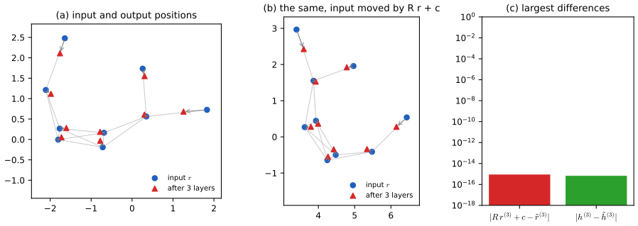
fig_13_s7. Download: PDF · SVGBuilding symmetries into architectures, translations for images, permutations for graphs, rotations and translations for molecules, is the subject of geometric deep learning (Bronstein et al. 2017, 2021).
Summary: errors and imprecisions found in the chapter (first printing)
- (13.21): the logarithm is missing; the loss is \(-\sum_n\sum_it_{ni}\ln y_{ni}\), not \(-\sum_n\sum_iy_{ni}^{t_{ni}}\) (Section 13.2.5; confirmed on a numerical example).
- (13.44), Exercise 13.6: the bias term is \(\one_N\bb^\T\) with \(\one_N\) of length \(N\) (one row per node), not \(\one_D\); with the column convention of (13.16) the weight matrices also appear transposed (Filling the gap 13.6).
- p. 411: "a 1 in position \(n,m\) indicates that node \(n\) will be relabelled as node \(m\)" is the inverse of what (13.3)–(13.4) do; the example (13.1) is an involution, which hides the difference (Result 13.1; a 3-cycle confirms it numerically).
- p. 417: deep sets as a graph "having no edges" with the sum "taken over all other vectors" is message passing on the complete graph (Filling the gap 13.5). The universal approximation statement for (13.15) needs a latent dimension that grows with the set size.
- p. 421: the requirement that the MLP of (13.28) be symmetric in its inputs is not needed for equivariance; and the equivalence of a graph attention network on a fully connected graph with a transformer encoder needs self-loops, the transformer's other sublayers, and no positional encodings (Result 13.7, Exercise 13.9).
- p. 416: (13.14) is attributed to Kipf and Welling; their GCN uses the renormalised matrix with self-loops, \(\tD^{-1/2}(\bA+\bI)\tD^{-1/2}\), which (13.14) is not (Filling the gap 13.4).
- p. 414: "The other eight 8 nodes" (a doubled number).
Exercises
All 10 exercises of Chapter 13 (Bishop and Bishop, 2024, pp. 425–427), restated in my own words, with complete solutions (hidden). Stars give the book's difficulty. The official solutions manual covers Chapters 2 to 10 only, so these solutions are my own, checked numerically where possible.
Exercise 13.1 (★). Show that the reordering \((A,B,C,D,E)\to(C,E,A,D,B)\) of Figure 13.2 is the transformation (13.5) with the permutation matrix (13.1).
Solution
New position \(n\) holds the old node \(\pi(n)\): \(C,E,A,D,B\) are old nodes \(3,5,1,4,2\), so \(\pi=(3,5,1,4,2)\) and by (13.3) the rows of \(\bP\) are \(\bu_3^\T,\bu_5^\T,\bu_1^\T,\bu_4^\T,\bu_2^\T\), which is (13.1). By Result 13.1(3), \((\bP\bA\bP^\T)_{nm}=A_{\pi(n)\pi(m)}\). For example the first row of \(\bP\bA\bP^\T\) is row \(C\) of \(\bA\) with its columns in the order \(C,E,A,D,B\): \((0,1,1,1,1)\), and the second is row \(E\): \((1,0,0,1,0)\), as in Figure 13.2(c). All 25 entries agree (checked).
Exercise 13.2 (★★). Show that the number of edges at each node is the corresponding diagonal element of \(\bA^2\).
Solution
\[(\bA^2)_{nn}=\sum_mA_{nm}A_{mn}=\sum_mA_{nm}^2=\sum_mA_{nm}=d_n,\] using the symmetry \(A_{mn}=A_{nm}\) and \(A_{nm}\in\{0,1\}\), so \(A_{nm}^2=A_{nm}\). In words, \((\bA^2)_{nn}\) counts walks \(n\to m\to n\) of length 2, one for each neighbour \(m\). (For a directed graph \((\bA^2)_{nn}\) would count the nodes linked in both directions; with self-loops each would add 1.) More generally \((\bA^k)_{nm}\) counts walks of length \(k\), and \(\Tr(\bA^3)/6\) counts triangles (45 in the karate club; checked).
Exercise 13.3 (★). Draw the graph with adjacency matrix \[ \bA=\begin{pmatrix}0&1&1&0&1\\1&0&1&1&1\\1&1&0&1&0\\0&1&1&0&0\\1&1&0&0&0\end{pmatrix}. \tag{13.42} \]
Solution
The matrix is symmetric with zero diagonal, so it is a simple undirected graph. Reading the upper triangle, with nodes \(A,\dots,E\): edges \(AB, AC, AE, BC, BD, BE, CD\), seven in all, and degrees \((3,4,3,2,2)\). It consists of the triangles \(ABC\), \(ABE\) and \(BCD\) sharing edges: \(B\) is linked to everything.
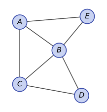
Exercise 13.3. The graph of (13.42), drawn by fig_13_ex3. Its only non-trivial symmetry swaps \(D\) and \(E\) while swapping \(A\) and \(C\), so it has \(120/2=60\) different adjacency matrices. Download: PDF · SVGExercise 13.4 (★★). Show that pre-multiplying a data matrix \(\bX\) by \(\bP\) of (13.3) permutes its rows according to \(\pi\), as in (13.4).
Solution
Row \(n\) of \(\bP\bX\) is (row \(n\) of \(\bP\)) times \(\bX\) \(=\bu_{\pi(n)}^\T\bX\), and \(\bu_k^\T\bX\) picks out row \(k\) of \(\bX\). So row \(n\) of \(\bP\bX\) is \(\bx_{\pi(n)}^\T\): \((\bP\bX)_{nj}=X_{\pi(n)j}\). (Result 13.1(2); checked for a random permutation.)
Exercise 13.5 (★★). Show that \(\widetilde\bA=\bP\bA\bP^\T\) (13.5) permutes both the rows and the columns of \(\bA\) according to \(\pi\).
Solution
By Exercise 13.4, \(\bP\bA\) has rows \(\ba_{\pi(n)}^\T\) (rows of \(\bA\) permuted). Post-multiplying by \(\bP^\T\) permutes columns: \((\bm B\bP^\T)_{nm}=\sum_kB_{nk}P_{mk}=B_{n\pi(m)}\). Together \((\bP\bA\bP^\T)_{nm}=A_{\pi(n)\pi(m)}\). Since the same \(\pi\) is applied to rows and columns, symmetry and the zero diagonal are preserved, and the result is the adjacency matrix of the same graph with the nodes renamed. (Result 13.1(3).)
Exercise 13.6 (★★). With \(\bH\) the \(N\times D\) matrix of rows \(\bh_n^\T\), show that the sums \(\bz_n=\sum_{m\in\nb(n)}\bh_m\) (13.43) form \(\bZ=\bA\bH\), and that the argument of the activation in (13.16) is, in matrix form, \(\bA\bH\bW_{\rm neigh}+\bH\bW_{\rm self}+\one_D\bb^\T\) (13.44).
Solution
\[(\bA\bH)_{nj}=\sum_mA_{nm}H_{mj}=\sum_{m\in\nb(n)}h_{mj}=z_{nj},\] so \(\bZ=\bA\bH\). Row \(n\) of the pre-activation is \[(\bW_{\rm self}\bh_n+\bW_{\rm neigh}\bz_n+\bb)^\T=\bh_n^\T\bW_{\rm self}^\T+\bz_n^\T\bW_{\rm neigh}^\T+\bb^\T;\] stacking rows gives \(\bH\bW_{\rm self}^\T+\bA\bH\bW_{\rm neigh}^\T+\one_N\bb^\T\). This is (13.44) if the weight matrices are stored transposed (as \(D\times D'\) matrices acting on row vectors), but the ones vector must be \(\one_N\), of length \(N\): \(\one_N\bb^\T\) puts the bias in every one of the \(N\) rows, while \(\one_D\bb^\T\) would be \(D\times D'\) and could not be added to an \(N\times D'\) matrix (Filling the gap 13.6; checked against the node-by-node layer).
Exercise 13.7 (★★). Using the layer equivariance (13.19) and (13.4), show that the whole network (13.18) is equivariant.
Solution
Let \(\bH^{(l)}\) be the outputs for \((\bX,\bA)\) and \(\widetilde\bH^{(l)}\) those for \((\bP\bX,\bP\bA\bP^\T)\). Claim: \(\widetilde\bH^{(l)}=\bP\bH^{(l)}\) for all \(l\). For \(l=0\), \(\widetilde\bH^{(0)}=\bP\bX=\bP\bH^{(0)}\) by (13.4). If it holds for \(l-1\), then \[\widetilde\bH^{(l)}=F(\widetilde\bH^{(l-1)},\bP\bA\bP^\T,\bW^{(l)})=F(\bP\bH^{(l-1)},\bP\bA\bP^\T,\bW^{(l)})=\bP\bH^{(l)}\] by (13.19). So \(\widetilde\bH^{(L)}=\bP\bH^{(L)}\), which is (13.7). The two ingredients are that every layer is equivariant for every input (not just for \(\bX\)) and that the same \(\bP\) acts on \(\bA\) in every layer. An invariant readout then makes the graph-level output invariant (Result 13.2; checked for a three-layer network).
Exercise 13.8 (★★). Explain why the aggregation (13.24) with attention weights (13.28) is equivariant under reordering of the nodes.
Solution
The weight \(A_{nm}\) is computed from the pair of vectors \((\bh_n,\bh_m)\) by an MLP shared by all pairs, and normalised over the neighbourhood of \(n\). Renaming nodes changes neither the vectors attached to a pair of nodes nor which nodes are neighbours, only their labels, so the weight between two given nodes is unchanged: \(\tilde A_{nm}=A_{\pi(n)\pi(m)}\), i.e. \(\widetilde{\bm{\mathcal A}}=\bP\bm{\mathcal A}\bP^\T\). Then \(\tilde\bz_n=\sum_m\tilde A_{nm}\tilde\bh_m=\sum_kA_{\pi(n)k}\bh_k=\bz_{\pi(n)}\), i.e. \(\widetilde\bZ=\bP\bZ\). The argument uses only that the MLP is shared, not that it is symmetric in its two arguments (Result 13.7; checked with an asymmetric score).
Exercise 13.9 (★). Show that a graph attention network on a fully connected graph is a standard transformer.
Solution
On a complete graph the neighbourhood of every node is every node (we must include \(n\) itself, i.e. add self-loops, because a transformer token attends to itself). The bilinear attention (13.27) with \(\bW=\bW_q\bW_k^\T/\sqrt{d_k}\) is then \(A_{nm}=\softmax_m(\bm q_n^\T\bm k_m/\sqrt{d_k})\) with \(\bm q_n=\bW_q^\T\bh_n\), \(\bm k_m=\bW_k^\T\bh_m\), the transformer's attention matrix; aggregating value vectors \(\bW_v^\T\bh_m\) by (13.24) gives the attention output \(\softmax(\bQ\bK^\T/\sqrt{d_k})\bm V\), and \(H\) heads with concatenation and a projection give multi-head attention. If the update (13.16) is chosen as the rest of a transformer layer (residual connection, layer normalisation, position-wise MLP), the layer is a transformer encoder layer. Neither architecture uses the node order, so without positional encodings both are permutation equivariant; a transformer with positional encodings is this graph network with positions included in the node features (Result 13.7; the attention part is checked to \(10^{-15}\)).
Exercise 13.10 (★★). A translated coordinate system gives
\[ \tilde\br=\br+\bc, \tag{13.45} \]and a rotated and/or reflected one
\[ \tilde\br=\bR\br, \tag{13.46} \]with \(\bR\) orthogonal,
\[ \bR\bR^\T=\bR^\T\bR=\bI. \tag{13.47} \]Show that under these transformations the quantities (13.38), (13.40) and (13.41) are invariant and the coordinates (13.39) equivariant.
Solution
Combine both: \(\tilde\br_n=\bR\br_n+\bc\). (i) \(\tilde\br_n-\tilde\br_m=\bR(\br_n-\br_m)\) and \(\|\bR\bv\|^2=\bv^\T\bR^\T\bR\bv=\|\bv\|^2\) by (13.47), so the squared distance in (13.38) is unchanged; all other inputs of (13.38) are unchanged too, so \(\be_{nm}^{(l+1)}\) is invariant, and so are \(\bz_n^{(l+1)}\) (13.40) and \(\bh_n^{(l+1)}\) (13.41), which are functions of invariant quantities. (ii) In (13.39), \(\phi(\be_{nm}^{(l+1)})\) is invariant, so \[\tilde\br_n^{(l+1)}=\bR\br_n+\bc+C\sum_m\bR(\br_n-\br_m)\phi=\bR\br_n^{(l+1)}+\bc:\] the new coordinates transform exactly as the old ones. Translations alone (\(\bR=\bI\)) and rotations/reflections alone (\(\bc=\bzero\)) are special cases. By induction the statements hold for every layer (Result 13.12, where it is also noted why the differences and the scalar weights are essential; checked to \(10^{-15}\)).
Demonstrations
Three interactive pages, each linked above where its topic arises. They run in the browser and reproduce the Python code (differences below \(2\times10^{-15}\) for the layer outputs, \(3\times10^{-14}\) relative for the propagated features, \(2\times10^{-14}\) relative for the training losses after 200 Adam steps; for the 16-layer network without residual connections rounding differences grow to \(2\times10^{-7}\) relative, with identical predictions).
- Reorder the nodes, compare the outputs: four graphs, seven layer types (sum, mean, Kipf, GCN, max, attention, and a broken position-tied layer), any reordering; the equivariance error, the sum readout, a network on the flattened adjacency matrix, and the count \(N!/|\mathrm{Aut}|\). Presets: 1 Figure 13.2, 2 flattened adjacency, 3 position-tied weights, 4 attention, 5 karate club, max.
- Message passing and over-smoothing: the receptive field of any node, repeated propagation with four normalisations, the distance to the limit against the bound \(\rho^k\), the Dirichlet energy, residual and initial-residual steps. Presets: 1 receptive field, 2 two communities, 3 collapse, 4 bipartite oscillation, 5 initial residual.
- A graph convolutional network, trained live: a GCN on the karate club with hand-written forward and backward passes and Adam; choose the labelled members, the depth, width, features and learning rate, with or without edges and residual connections. Presets: 1 two labels, 2 no edges, 3 width-2 hidden layer, 4 sixteen plain layers, 5 sixteen residual layers.
References
- Bishop, C. M. and Bishop, H. (2024). Deep Learning: Foundations and Concepts. Springer, Cham. Chapter 13, pp. 407–427. doi:10.1007/978-3-031-45468-4. Book website: www.bishopbook.com.
- Battaglia, P. W. et al. (2018). Relational inductive biases, deep learning, and graph networks. arXiv:1806.01261.
- Bronstein, M. M., Bruna, J., LeCun, Y., Szlam, A. and Vandergheynst, P. (2017). Geometric deep learning: going beyond Euclidean data. IEEE Signal Processing Magazine, 34(4), 18–42.
- Bronstein, M. M., Bruna, J., Cohen, T. and Veličković, P. (2021). Geometric deep learning: grids, groups, graphs, geodesics, and gauges. arXiv:2104.13478.
- Cai, C. and Wang, Y. (2020). A note on over-smoothing for graph neural networks. arXiv:2006.13318.
- Chung, F. R. K. (1997). Spectral Graph Theory. American Mathematical Society.
- Defferrard, M., Bresson, X. and Vandergheynst, P. (2016). Convolutional neural networks on graphs with fast localized spectral filtering. In Advances in Neural Information Processing Systems 29.
- Gasteiger (Klicpera), J., Bojchevski, A. and Günnemann, S. (2019). Predict then propagate: graph neural networks meet personalized PageRank. In International Conference on Learning Representations.
- Gilmer, J., Schoenholz, S. S., Riley, P. F., Vinyals, O. and Dahl, G. E. (2017). Neural message passing for quantum chemistry. In Proceedings of the 34th International Conference on Machine Learning, 1263–1272.
- Hamilton, W. L. (2020). Graph Representation Learning. Morgan & Claypool.
- Hammond, D. K., Vandergheynst, P. and Gribonval, R. (2011). Wavelets on graphs via spectral graph theory. Applied and Computational Harmonic Analysis, 30(2), 129–150.
- Kipf, T. N. and Welling, M. (2017). Semi-supervised classification with graph convolutional networks. In International Conference on Learning Representations (arXiv:1609.02907, 2016).
- Morris, C., Ritzert, M., Fey, M., Hamilton, W. L., Lenssen, J. E., Rattan, G. and Grohe, M. (2019). Weisfeiler and Leman go neural: higher-order graph neural networks. In Proceedings of the AAAI Conference on Artificial Intelligence, 33, 4602–4609.
- Oono, K. and Suzuki, T. (2020). Graph neural networks exponentially lose expressive power for node classification. In International Conference on Learning Representations.
- Rong, Y., Huang, W., Xu, T. and Huang, J. (2020). DropEdge: towards deep graph convolutional networks on node classification. In International Conference on Learning Representations.
- Satorras, V. G., Hoogeboom, E. and Welling, M. (2021). E(n) equivariant graph neural networks. In Proceedings of the 38th International Conference on Machine Learning, 9323–9332.
- Veličković, P., Cucurull, G., Casanova, A., Romero, A., Liò, P. and Bengio, Y. (2018). Graph attention networks. In International Conference on Learning Representations (arXiv:1710.10903, 2017).
- Veličković, P. (2023). Everything is connected: graph neural networks. Current Opinion in Structural Biology, 79, 102538.
- Wagstaff, E., Fuchs, F., Engelcke, M., Posner, I. and Osborne, M. A. (2019). On the limitations of representing functions on sets. In Proceedings of the 36th International Conference on Machine Learning, 6487–6494.
- Wu, Z., Pan, S., Chen, F., Long, G., Zhang, C. and Yu, P. S. (2019). A comprehensive survey on graph neural networks. arXiv:1901.00596.
- Xu, K., Li, C., Tian, Y., Sonobe, T., Kawarabayashi, K. and Jegelka, S. (2018). Representation learning on graphs with jumping knowledge networks. In Proceedings of the 35th International Conference on Machine Learning, 5453–5462.
- Xu, K., Hu, W., Leskovec, J. and Jegelka, S. (2019). How powerful are graph neural networks? In International Conference on Learning Representations.
- Zachary, W. W. (1977). An information flow model for conflict and fission in small groups. Journal of Anthropological Research, 33(4), 452–473.
- Zaheer, M., Kottur, S., Ravanbakhsh, S., Póczos, B., Salakhutdinov, R. and Smola, A. J. (2017). Deep sets. In Advances in Neural Information Processing Systems 30.
- Zhou, J., Cui, G., Zhang, Z., Yang, C., Liu, Z. and Sun, M. (2018). Graph neural networks: a review of methods and applications. arXiv:1812.08434.
Every numerical statement in these notes comes from ch13_graph_neural_networks.py; the demos' graphs and features are in data/ch13-graphs.json.