Convolutional Networks
A fully connected network treats an image as an unordered list of numbers. A convolutional network builds in what we know about images instead: nearby pixels belong together (locality), the same pattern means the same thing wherever it appears (translation equivariance through shared weights), small displacements should not change the answer (invariance through pooling), and complex objects are made of simpler parts (hierarchy through depth). This chapter develops the convolutional layer and its arithmetic (Section 10.2), looks inside trained networks with filters, saliency maps and adversarial examples (10.3), and applies convolutional networks to object detection (10.4), segmentation with up-sampling layers (10.5) and style transfer (10.6).
Ch. 1 Deep learning revolution Ch. 2 Probabilities Ch. 3 Standard distributions Ch. 4 Regression Ch. 5 Classification Ch. 6 Deep neural networks Ch. 7 Gradient descent Ch. 8 Backpropagation Ch. 9 Regularization Ch. 10 Convolutional networks Ch. 11 Structured distributions Ch. 12 Transformers Ch. 13 Graph neural networks Ch. 14 Sampling Ch. 15 Discrete latent variables Ch. 16 Continuous latent variables Ch. 17 GANs Ch. 18 Normalizing flows Ch. 19 Autoencoders Ch. 20 Diffusion models Appendices A to C
How to read these notes
They follow the book. Sections carry the book's numbers (10.1, 10.2.4, ...) and every displayed equation that appears in the book carries the book's own equation number, e.g. (10.5), so the notes can be read next to the book. Equations without a number are steps that the book skips.
Filling the gaps. Wherever the book states a result without proof, says it "can be shown", or leaves it to an exercise, an orange Filling the gap box or a proof gives the full argument. Proofs and derivations start hidden: open one with its bar, or use the button below.
Figures and demonstrations. Seventeen figures of the chapter are computed by the Python code. Where the book shows a large network trained on ImageNet (Figures 10.12 to 10.18 and 10.32), the same phenomenon is reproduced at small scale with one convolutional network of 17,347 parameters trained on MNIST on a laptop CPU; the captions say so. Two supplementary figures (10.S1, 10.S2, our own) measure equivariance, invariance and adversarial robustness. The ▶ Demo boxes open an interactive demonstration already set to the case being discussed.
Main reference
C. M. Bishop and H. Bishop, Deep Learning: Foundations and Concepts, Springer (2024), Chapter 10, pages 287–324. Section, equation, figure and exercise numbers below refer to this book. Further reading is listed in the references; the book's website is www.bishopbook.com.
The explanations, derivations, figures and code are my own; equations are cited by their numbers in the book.
Companion course: Bayesian and Probabilistic Machine Learning
Part of this chapter overlaps the companion course Bayesian and Probabilistic Machine Learning (Bishop 2006). Where the full proof is already there, these notes give the statement and a short argument and link it.
- Convolutional networks in Bishop (2006): local receptive fields, weight sharing, subsampling, shift equivariance and the parameter count: Section 5.5.6, Result 5.16 (here 10.2.2, Result 10.1, 10.2.6).
- Four routes to invariance (augmentation, regularisation, invariant features, architecture), tangent propagation and training with transformed data: Sections 5.5.3, 5.5.4 and 5.5.5 (here the introduction to 10.2 and Filling the gap 10.8).
- Backpropagation, and summing the derivatives of tied (shared) weights: Section 5.3.1 and Filling the gap 5.5 (here Result 10.4, the backward pass of a convolution).
- The Jacobian of a network with respect to its inputs, which saliency maps and adversarial perturbations use: Section 5.3.4 (here 10.3.3 and 10.3.4).
- Softmax outputs and multiclass logistic regression: Section 4.3.4 (here Filling the gap 10.10 and 10.4.1); Lagrange multipliers: toolkit, Section 2.1 (here Exercise 10.1); the product rule: Section 1.2 (here Exercise 10.11).
- Demonstration: the backpropagation demo; here the adversarial demo backpropagates to the input pixels instead of the weights.
The chapter at a glance
- 10.2 A convolutional layer is a sparse, weight-shared linear map followed by a nonlinearity. It commutes with translations, and every translation-commuting linear map is a convolution (Result 10.1). Its output size is \(\floor{(J+2P-D(M-1)-1)/S}+1\) (Result 10.2; the printed (10.5) has a sign error). Its backward pass is again a convolution, with the flipped kernel, and for strides a transposed convolution (Result 10.4). Receptive fields grow linearly with depth, exponentially with dilation, and the effective receptive field only like \(\sqrt{L}\) (Result 10.3). Pooling turns equivariance into (approximate) invariance (Filling the gap 10.8).
- 10.3 First-layer filters look like Gabor functions, whose spectrum is concentrated at one orientation and frequency (Filling the gap 10.9). Grad-CAM, exactly a decomposition of the class score for a global-average-pooling head (Result 10.5). The fast gradient sign method is the best first-order attack of max-norm \(\epsilon\), and in \(D\) dimensions it beats a random perturbation by a factor of order \(\sqrt D\) (Result 10.6).
- 10.4 IoU and its metric \(1-\IoU\) (Result 10.7); sliding windows are a convolution, with windows spaced by the product of the strides (Result 10.8); non-max suppression (Algorithm 10.3), run on real detections of our network.
- 10.5–10.6 Unpooling, max-unpooling and transposed convolutions are the adjoints of pooling and convolution (Result 10.9). Style is matched through the Gram matrix of the features, whose gradient is derived in Result 10.10.
Notation. Images and feature maps are arrays \(X_{c,j,k}\) with channel \(c\) and pixel \((j,k)\); indices start at 0. A filter has size \(M\times M\) (or \(L\times M\)), padding \(P\), stride \(S\) and dilation \(D\). A layer has \(C\) input and \(C_{\rm out}\) output channels. \(a\) denotes pre-activations, \(z=\ReLU(a)\) activations, \(a^{(c)}\) the pre-softmax output for class \(c\), and \(E\) an error function. \(T_{\bm s}\) is the translation by \(\bm s=(s_1,s_2)\): \((T_{\bm s}X)_{j,k}=X_{j-s_1,k-s_2}\).
The network used in the figures. Three convolutional layers (16, 24 and 32 channels; filters 5×5, 5×5, 3×3; 'same' padding; ReLU; 2×2 max-pooling after the first two), a global max-pooling over positions and a linear layer with 11 outputs: the ten digits and a background class (digits shifted out of the centre of the window, as in Exercise 10.11), so that the same network can be scanned over a larger image. 17,347 parameters; 98.4% test accuracy on the ten digits after three epochs (three and a half minutes on one CPU thread).
Printings. The first printing has a few slips in this chapter (a sign in (10.5), a missing flip in (10.20), a stride in Section 10.4.3, a statement about where VGG-16's connections are, and a label in (10.16)); two numbers in the solutions manual are also off. Each is flagged with an Erratum note where it occurs and listed with the evidence in the summary at the end of Section 10.6.
pp. 287–288 The models of the earlier chapters treat the input \(\bx=(x_1,\dots,x_D)\) as unstructured: apply one fixed permutation to the coordinates of every training and test vector and nothing changes. Images, sound and text are not like that: pixels sit on a grid, and nearby pixels are strongly correlated. The book's way of exploiting this structure in Chapter 10 is architectural: a convolutional neural network (CNN), a sparsely connected network with shared parameters, built to respect translations of the image. (The alternatives, regularisation and data augmentation, are the subject of Section 9.1 of the book.)
Filling the gap 10.1: a fully connected network cannot use the order of its inputs p. 287
The book asserts that permuting the input variables makes no difference to the models considered so far. Here is the precise statement for a network whose first layer is fully connected, trained by gradient descent from weights drawn independently from one distribution.
Derivation
Let \(\bPi\) be a \(D\times D\) permutation matrix, so \(\bPi^\T\bPi=\bI\). The first layer computes \(\ba=\bW\bx+\bb\). If every input is replaced by \(\bPi\bx\), the network with first-layer weights \(\bW'=\bW\bPi^\T\) computes \(\bW'\bPi\bx+\bb=\bW\bx+\bb\): the same pre-activations, hence the same outputs and the same error, \(E'(\bW')=E(\bW)\) for the permuted data. The map \(\bW\mapsto\bW\bPi^\T\) is a bijection (it permutes the columns), so the two error surfaces are the same surface in permuted coordinates.
Training. By the chain rule \(\nabla_{\bW'}E'=\nabla_{\bW}E\,\bPi^\T\). Hence if \(\bW'^{(0)}=\bW^{(0)}\bPi^\T\), one gradient step gives \(\bW'^{(1)}\)\({}=\bW'^{(0)}-\eta\nabla_{\bW'}E'\)\({}=(\bW^{(0)}-\eta\nabla_\bW E)\bPi^\T\)\({}=\bW^{(1)}\bPi^\T\), and by induction the two runs stay in correspondence for ever (also for momentum and Adam, whose updates act element by element, and for mini-batches drawn in the same order). Finally, if the initial weights are independent and identically distributed, \(\bW^{(0)}\bPi^\T\) has the same distribution as \(\bW^{(0)}\). So the trained network on permuted pixels has exactly the same distribution of predictions as on the original pixels: no information about the arrangement of the pixels can enter. A convolutional layer breaks this symmetry on purpose, since its weight matrix is constrained to a form (Filling the gap 10.4) that is not preserved by column permutations. ∎
10.1 Computer vision
pp. 288–289 Computer vision, the automatic analysis of images, was built for decades on projective geometry and hand-crafted features fed into simple learning algorithms; it was among the first fields to be transformed by deep learning, mainly through CNNs (transformers, Chapter 12 of the book, are now competitive in some tasks). The book lists ten typical tasks: classification (one label per image), detection (find and locate objects, Section 10.4), segmentation (a label per pixel, Section 10.5), caption generation, image synthesis, inpainting, style transfer (Section 10.6), super-resolution, depth prediction and three-dimensional scene reconstruction.
10.1.1 Image data
p. 289 An image is a rectangular array of pixels, each a grey value or a triple of red, green and blue intensities, non-negative and bounded (often 8-bit integers \(0,\dots,255\)); MRI scans are three-dimensional arrays of voxels and videos are stacks of frames. Two facts make a generic network a poor fit. Images are large (tens of megapixels), so a dense first layer would need an infeasible number of weights; and images are highly structured: randomly permuting the pixels of a photograph destroys it, and an image with independently drawn pixels is essentially never a natural image (compare the random images in Figure 6.8 of Chapter 6). Nearby pixels have similar values much more often than distant ones. This is strong prior knowledge, and building it into the network gives far fewer parameters and better generalisation.
10.2 Convolutional Filters
See also the companion course, Section 5.5.3 (four ways to obtain invariance) and Section 5.5.6 (convolutional networks).
p. 290 For a colour image of \(10^3\times10^3\) pixels and a first hidden layer of 1,000 units, a fully connected layer already has \(3\times10^9\) weights, and it would have to learn from examples that a cat in the corner is still a cat. Four related ideas lead to a better architecture: hierarchy (faces are made of eyes, eyes of irises, irises of edges), locality (low-level features can be detected from small patches), equivariance (a feature detector should work in the same way at every position) and invariance (the class label should not change when the object moves a little). The hierarchy is built in; what is detected at each level is learned from data, end to end.
10.2.1 Feature detectors
pp. 290–291 Take a grey-scale image and one hidden unit connected only to a small patch of pixels, its receptive field (Figure 10.1, a diagram). With the pixel values of the patch in a vector \(\bx\),
\[ z=\ReLU(\bw^\T\bx+w_0). \tag{10.1} \]The weights form a small two-dimensional array, the filter or kernel, which can be displayed as an image.
Filling the gap 10.2: a filter responds most strongly to a patch that looks like itself p. 291; Exercise 10.1
The book states that among patches of fixed norm the response \(\bw^\T\bx\) is largest for \(\bx=\alpha\bw\), and that the ReLU unit "fires" when the match is good enough. Both statements in full:
Derivation
Maximum. Fix \(\|\bx\|=r>0\) and \(\bw\ne\bzero\). By the Cauchy–Schwarz inequality \(\bw^\T\bx\le\|\bw\|\,\|\bx\|=r\|\bw\|\), with equality if and only if \(\bx\) is a non-negative multiple of \(\bw\); with the norm fixed, \(\bx=r\bw/\|\bw\|\). (With a Lagrange multiplier, as Exercise 10.1 asks: stationary points of \(\bw^\T\bx-\lambda(\|\bx\|^2-r^2)\) satisfy \(\bw=2\lambda\bx\), so \(\bx=\pm r\bw/\|\bw\|\); the plus sign is the maximum and the minus sign the minimum. See the toolkit of the companion course for the method.) The filter, read as an image, is therefore the patch of given contrast that excites the unit most.
Threshold. Write \(\bw^\T\bx=\|\bw\|\,\|\bx\|\cos\theta\), with \(\theta\) the angle between the patch and the filter. The unit (10.1) is non-zero exactly when \(\bw^\T\bx>-w_0\), that is when \(\cos\theta>-w_0/(\|\bw\|\,\|\bx\|)\). For \(w_0<0\) this is a matched filter with a threshold: the patch must point close enough to the direction of \(\bw\), and the required closeness relaxes for high-contrast patches (large \(\|\bx\|\)). Note that subtracting the mean from the image (Section 10.2.3) matters here: a bright uniform patch has a large norm but carries no pattern. ∎
10.2.2 Translation equivariance
pp. 291–294 An eye is an eye wherever it is in the image, so the unit that detects it at one position should be copied, with the same weights, to every position. The copies form a feature map; the connections are sparse (each unit sees only its patch) and shared (Figure 10.2, a diagram: six connections, two parameters). In two dimensions the feature map is
\[ C(j,k)=\sum_l\sum_mI(j+l,k+m)K(l,m), \tag{10.2} \]written \(C=I*K\) (the nonlinearity is omitted). Strictly, (10.2) is a cross-correlation; the convolution of mathematics flips the kernel. Machine learning calls both "convolution".
Definition 10.1 (cross-correlation and convolution) pp. 292, 322, (10.2), (10.19)
For an image \(I\) of size \(J\times K\) and a kernel \(K\) of size \(L\times M\), indices from 0, the cross-correlation (the book's "convolution") and the convolution are
\[ (I\star K)(j,k)=\sum_{l=0}^{L-1}\sum_{m=0}^{M-1}I(j+l,k+m)\,K(l,m),\qquad (I*K)(j,k)=\sum_{l=0}^{L-1}\sum_{m=0}^{M-1}I(j-l,k-m)\,K(l,m). \]In the "valid" range, where every term exists, \(0\le j\le J-L\), \(0\le k\le K-M\) for \(\star\) and \(L-1\le j\le J-1\), \(M-1\le k\le K-1\) for \(*\) (Exercise 10.4). The two are related by flipping the kernel: \(I*K=I\star\widetilde K\) up to a shift of the indices, with \(\widetilde K(l,m)=K(L-1-l,M-1-m)\).
Filling the gap 10.3: convolution versus cross-correlation, and why learning does not care p. 292; Exercises 10.4, 10.5
The book notes the difference and moves on. Three facts make the choice harmless, and one makes convolution the "right" mathematical object.
Derivation
Flip. Substitute \(l'=L-1-l\), \(m'=M-1-m\) in the convolution: \[(I*K)(j,k)=\sum_{l',m'}I(j-L+1+l',\,k-M+1+m')\,\widetilde K(l',m')=(I\star\widetilde K)(j-L+1,\,k-M+1).\] So the valid convolution equals the valid cross-correlation with the flipped kernel, re-indexed to start at 0.
Learning. Flipping is a bijection on kernels. A network with cross-correlation layers and kernels \(K\) computes exactly the same function as one with convolution layers and kernels \(\widetilde K\); the error surfaces correspond, gradient descent commutes with the bijection (as in Filling the gap 10.1), and an i.i.d. initialisation is flip-invariant in distribution. The trained network just stores its kernels upside down.
Algebra. Convolution of finitely supported arrays (the 'full' version, zero outside the support) is commutative and associative: \((I*K)(\bm n)\)\({}=\sum_{\bm p}I(\bm n-\bm p)K(\bm p)\)\({}=\sum_{\bm q}I(\bm q)K(\bm n-\bm q)\)\({}=(K*I)(\bm n)\) with \(\bm q=\bm n-\bm p\), and \(((I*K_1)*K_2)(\bm n)\)\({}=\sum_{\bm p,\bm q}I(\bm n-\bm p-\bm q)K_1(\bm p)K_2(\bm q)\) is symmetric in the two kernels' roles. Hence two convolutional layers without a nonlinearity in between are a single convolution with kernel \(K_1*K_2\) (which is how receptive fields add up, Section 10.2.7). Cross-correlation is not commutative: \(K_1\star K_2\) is the flip of \(K_2\star K_1\).
Exercise 10.5. The continuous convolution \(F(x)=\int G(y)k(x-y)\,\d y\) evaluated at \(x=j\Delta\) and approximated by a Riemann sum with \(y=(j-l)\Delta\) (substituting \(z=x-y\)) is \(F(j\Delta)\)\({}\approx\sum_lG((j-l)\Delta)\,k(l\Delta)\,\Delta\), which is (10.19) in one dimension with \(I(n)=G(n\Delta)\) and \(K(l)=k(l\Delta)\Delta\). A numerical test confirms this on two Gaussians, whose convolution is the Gaussian with the variances added (error below \(10^{-6}\) for \(\Delta=0.01\)). ∎
The feature map inherits a symmetry from the sharing of weights: shift the input, and the map shifts with it.
Result 10.1 (translation equivariance, and its converse) pp. 291–292
- Let a layer compute \(a_{o,\bm n}\)\({}=b_o+\sum_c\sum_{\bm p}W_{o,c,\bm p}\,X_{c,\bm n+\bm p}\) followed by an element-wise nonlinearity \(h\), with \(\bm n,\bm p\in\Z^2\) and the image extended periodically (circular padding) or defined on all of \(\Z^2\). Then for every translation \(T_{\bm s}\), \[h(a(T_{\bm s}X))=T_{\bm s}\,h(a(X)).\] With zero padding the identity holds at every output position whose receptive field, in both images, avoids the padding.
- Conversely, on signals of length \(n\) with circular boundary, a linear map \(\bA\) commutes with the cyclic shift \(\bS\) if and only if \(\bA=\sum_{k=0}^{n-1}c_k\bS^k\) (a circulant matrix), that is, iff \(\bA\) is a circular convolution with the kernel \(c\). The same holds in two dimensions with two shifts.
Proof
(1) \(a(T_{\bm s}X)_{o,\bm n}\)\({}=b_o+\sum_{c,\bm p}W_{o,c,\bm p}X_{c,\bm n+\bm p-\bm s}\)\({}=a(X)_{o,\bm n-\bm s}\)\({}=(T_{\bm s}a(X))_{o,\bm n}\): the weights do not depend on \(\bm n\), so only the argument moves. The nonlinearity acts position by position, so it commutes with any permutation of positions, in particular with \(T_{\bm s}\). Under zero padding, \(T_{\bm s}X\) is \(X\) moved with zeros shifted in; the computation of \(a_{o,\bm n}\) uses only the inputs in its receptive field, and where these coincide in both images the two sums agree. A composition of equivariant layers is equivariant, so the whole stack of convolutional layers is.
(2) If \(\bA=\sum_kc_k\bS^k\) it commutes with \(\bS\) because powers of \(\bS\) do. Conversely suppose \(\bA\bS=\bS\bA\) and let \(\be_0\) be the first unit vector; then \(\be_k=\bS^k\be_0\). Put \(c=\bA\be_0\) (the first column) and \(\bB=\sum_kc_k\bS^k\). Then \(\bB\be_0=\sum_kc_k\be_k=c=\bA\be_0\), and for every \(j\), \(\bA\be_j\)\({}=\bA\bS^j\be_0\)\({}=\bS^j\bA\be_0\)\({}=\bS^j\bB\be_0\)\({}=\bB\bS^j\be_0\)\({}=\bB\be_j\). So \(\bA=\bB\). In particular the commutant of \(\bS\) is \(n\)-dimensional, which a numerical test confirms by computing the null space of \(\bA\mapsto\bA\bS-\bS\bA\) for \(n=8\). Thus weight sharing is not just one way to get equivariance: among linear layers on a periodic grid it is the only way. ∎
Filling the gap 10.4: a convolutional layer is a sparse, weight-shared fully connected layer pp. 292–294; Exercise 10.2
The book says the connections are sparse and the weights shared. Written as a matrix:
Derivation
One dimension. A width-3 filter \((k_1,k_2,k_3)\) on an input \(\bx\in\R^5\) with stride 1 and no padding gives 3 outputs, \(y_i=k_1x_i+k_2x_{i+1}+k_3x_{i+2}\), that is \(\by=\bA\bx\) with \[ \bA=\begin{pmatrix}k_1&k_2&k_3&0&0\\0&k_1&k_2&k_3&0\\0&0&k_1&k_2&k_3\end{pmatrix}. \] Missing connections are zeros (sparsity: 9 of 15 entries non-zero) and shared weights are repeated entries: \(\bA\) is constant along its diagonals, a Toeplitz matrix. A dense layer would have 15 free weights; this one has 3.
Two dimensions. Order the pixels row by row. The output row \(j\) depends on input rows \(j,\dots,j+L-1\), and the block linking output row \(j\) to input row \(j+l\) is the one-dimensional Toeplitz matrix of the kernel row \(K(l,\cdot)\). So the full matrix is block Toeplitz with Toeplitz blocks. For a \(J\times K\) image and an \(M\times M\) filter (valid, stride 1), the dense layer between the same two arrays would have \(JK(J-M+1)(K-M+1)\) weights; the convolution has \((J-M+1)(K-M+1)M^2\) non-zero entries ("connections") but only \(M^2\) distinct values (plus one bias). For \(224\times224\) colour images and 64 output channels with \(3\times3\) filters: a dense layer to a \(224\times224\times64\) map would need \(4.8\times10^{11}\) weights; the convolution has 1,792 parameters.
Consequences. The matrix view makes the backward pass immediate: the gradient with respect to the input is \(\bA^\T\) applied to the output gradient, and \(\bA^\T\) is again sparse and weight-shared (Result 10.4). It also explains the three advantages listed by the book on pp. 293–294: few weights (sparsity), fewer parameters to learn (sharing, hence less data needed), and independence of the image size (the same \(M^2\) numbers define \(\bA\) for any \(J,K\)). ∎
Batch normalisation in a CNN. p. 292 When batch normalisation (Section 7.4.2) is used after a convolutional layer, one mean and one variance per channel are computed over the mini-batch and all positions, and one pair of learned scale and shift parameters is used per channel. Per-position statistics would break equivariance; per-channel statistics preserve it, because averaging over all positions is unchanged by a (circular) shift, so the normalised map of a shifted input is the shifted normalised map (checked numerically).
Edge detection. pp. 292–293 A vertical edge is a large change of intensity along a row. The fixed filters
\[ \begin{pmatrix}-1&0&1\\-1&0&1\\-1&0&1\end{pmatrix}, \tag{10.3} \] \[ \begin{pmatrix}-1&-1&-1\\0&0&0\\1&1&1\end{pmatrix} \tag{10.4} \]respond to vertical and horizontal edges: the response of (10.3) at a pixel is the sum over three rows of (right neighbour minus left neighbour), a smoothed horizontal derivative, positive where the intensity increases from left to right and negative where it decreases (Figure 10.4).
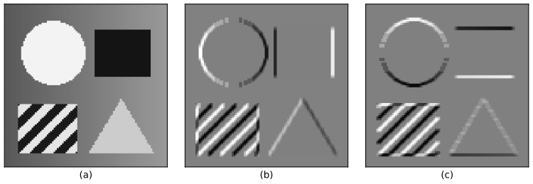
Figure 10.3 of the book is a symbolic worked example (a \(3\times3\) image with a \(2\times2\) filter); its numerical counterpart is Exercise 10.3, and a numerical test confirms the symbolic entries \(aj+bk+dl+em,\dots\) on random numbers.
10.2.3 Padding
p. 294 A \(J\times K\) image and an \(M\times M\) filter give a \((J-M+1)\times(K-M+1)\) map (the filter must fit). Padding the image with \(P\) pixels on every side (Figure 10.5, a diagram) gives \((J+2P-M+1)\times(K+2P-M+1)\). With \(P=0\) the convolution is valid; with \(P=(M-1)/2\) for odd \(M\) it is same, since \(J+2\cdot\frac{M-1}2-M+1=J\) (Exercise 10.6). Odd filter sizes give symmetric padding and a central pixel. Padding values are usually zero, after subtracting the mean intensity so that zero means "average".
10.2.4 Strided convolutions
p. 294 To shrink the map, move the filter \(S\) pixels at a time, the stride. The number of positions along an axis is counted in the next result; for large images the map is about \(1/S\) of the image size in each direction.
Result 10.2 (size of a feature map) p. 294, (10.5); Exercises 10.6, 10.7
Along an axis of length \(J\), padding \(P\), a filter of size \(M\), stride \(S\) and dilation \(D\) (the taps \(D\) pixels apart, Filling the gap 10.6) give
\[ J_{\rm out}=\floor{\frac{J+2P-D(M-1)-1}{S}}+1 \]outputs, provided \(J+2P\ge D(M-1)+1\). With \(D=1\) the map has \(\floor{(J+2P-M)/S+1}\)\({}\times\floor{(K+2P-M)/S+1}\) units, which is (10.5) corrected.
Erratum. The first printing has \(-1\) inside the floor in (10.5): \(\floor{(J+2P-M)/S-1}\). That is wrong by 2: for the example of Figure 10.3 (\(J=3\), \(M=2\), \(P=0\), \(S=1\)) it gives 0 instead of 2, and for \(J=4\) it gives 1 instead of 3. The solutions manual (Solution 10.7) has the correct \(+1\).
Proof (Exercises 10.6 and 10.7)
After padding, the axis has \(J'=J+2P\) positions \(0,\dots,J'-1\). A filter whose first tap is at \(p\) covers \(p,p+D,\dots,p+D(M-1)\), so it fits iff \(p+D(M-1)\le J'-1\), i.e. \(0\le p\le J'-1-D(M-1)\). With stride \(S\) the first taps are \(p=0,S,2S,\dots\); the admissible ones are \(p=iS\) with \(0\le i\le(J'-1-D(M-1))/S\), and there are \(\floor{(J'-1-D(M-1))/S}+1\) such integers \(i\). Substituting \(J'\) gives the formula; for \(D=1\) it is \(\floor{(J+2P-M)/S}+1\), and the \(+1\) (the first position) can be moved inside the floor because it is an integer. A numerical test compares the formula with the actual array sizes produced by our cross-correlation and by PyTorch for 1,440 combinations of \(J,M,P,S,D\). ∎
Filling the gap 10.5: a strided convolution is a subsampled convolution, and it is equivariant only to shifts by multiples of the stride p. 294
Derivation
Write \(C^{(1)}\) for the stride-1 map. From the proof of Result 10.2, the stride-\(S\) map is \(C^{(S)}(i,i')=C^{(1)}(iS,i'S)\): computing \(C^{(1)}\) and keeping every \(S\)-th row and column gives the same numbers at about \(S^2\) times the cost, which is why strides are used for down-sampling.
Equivariance. By Result 10.1, shifting the input by \(\bm s\) shifts \(C^{(1)}\) by \(\bm s\). If \(\bm s=S\bm t\) with integer \(\bm t\), then \(C^{(S)}(T_{\bm s}X)(\bm i)\)\({}=C^{(1)}(X)(S\bm i-S\bm t)\)\({}=C^{(S)}(X)(\bm i-\bm t)\): the strided map shifts by \(\bm t\). For other shifts the subsampling grid picks different samples of \(C^{(1)}\), and the strided map of the shifted image is in general not a shift of the original strided map (it changes, a form of aliasing). The same is true of pooling with stride \(S\) (Filling the gap 10.8) and is why a CNN with total stride 4 is exactly equivariant only to shifts by multiples of 4 pixels; Figure 10.S1 measures what happens in between. ∎
Filling the gap 10.6: dilated convolutions (not in the book; used in Section 10.5 architectures)
A dilated (or atrous) convolution spaces the filter taps \(D\) pixels apart: \(C(j,k)=\sum_{l,m}I(j+Dl,\,k+Dm)K(l,m)\). It enlarges the receptive field without adding weights or reducing resolution, which is useful for segmentation (Yu and Koltun, 2016).
Derivation
Equivalence. A dilated filter is an ordinary filter of size \(D(M-1)+1\) with zeros between the taps, \(K_D(Dl,Dm)=K(l,m)\) and 0 elsewhere, so everything said about convolutions applies, including equivariance (Result 10.1) and the size formula with \(M\) replaced by \(D(M-1)+1\) (Result 10.2).
Exponential receptive fields. Stack \(L\) layers of \(3\times3\) filters with dilations \(1,2,4,\dots,2^{L-1}\) and stride 1. By the recursion of Result 10.3 the receptive field is \(r_L=1+\sum_{l=1}^{L}2\cdot2^{l-1}=2^{L+1}-1\), while the parameter count grows only linearly in \(L\). Moreover there are no holes: the composite filter is the convolution of the dilated filters (Filling the gap 10.3), whose support in one dimension is \(\{\sum_l\epsilon_l2^{l-1}:\epsilon_l\in\{-1,0,1\}\}\), which is every integer in \([-(2^L-1),2^L-1]\): write \(|n|\) in binary with \(L\) digits and give every non-zero digit the sign of \(n\). Figure 10.9 shows the three-layer case. ∎
10.2.5 Multi-dimensional convolutions
pp. 295–296 A colour image is a \(J\times K\times C\) tensor (Section 6.3.7), and a filter for it is an \(M\times M\times C\) tensor, one \(M\times M\) slice per input channel (Figure 10.6, a diagram). One such filter gives one feature map, as one hidden unit of a dense layer gives one number; to detect many features we use \(C_{\rm out}\) filters, each with its own bias, and get \(C_{\rm out}\) feature maps, again called channels (Figure 10.7, a diagram). The filter tensor is \(M\times M\times C\times C_{\rm out}\) and the layer has \((M^2C+1)C_{\rm out}\) parameters, whatever the image size.
Definition 10.2 (convolutional layer) pp. 295–296, 298
With input \(X\in\R^{C\times J\times K}\), weights \(W\in\R^{C_{\rm out}\times C\times M\times M}\), biases \(b\in\R^{C_{\rm out}}\), zero padding \(P\), stride \(S\) and dilation \(D\), the pre-activations are
\[ a_{o,j,k}=b_o+\sum_{c=0}^{C-1}\sum_{l=0}^{M-1}\sum_{m=0}^{M-1}W_{o,c,l,m}\,X^{\rm pad}_{c,\,jS+lD,\,kS+mD}, \]with \(X^{\rm pad}\) the padded input and \((j,k)\) ranging over the sizes of Result 10.2; the activations are \(z=h(a)\) element by element. Our numpy conv_forward implements exactly this and agrees with PyTorch's conv2d (checked with stride 2, padding 1 and dilation 2).
Filling the gap 10.7: a convolutional layer is one matrix product, and a 1×1 convolution is a dense layer applied at every pixel pp. 295–296
Derivation
The matrix product. Collect, for every output position \((j,k)\), the \(CM^2\) inputs of its receptive field into a column; the \(J_{\rm out}K_{\rm out}\) columns form a matrix \(\bX_{\rm col}\in\R^{CM^2\times J_{\rm out}K_{\rm out}}\) ("im2col"). Reshape the weights to \(\bW_{\rm mat}\in\R^{C_{\rm out}\times CM^2}\). Then Definition 10.2 reads \[\bA=\bW_{\rm mat}\bX_{\rm col}+\bb\one^\T,\] one matrix product with \(C_{\rm out}\,CM^2\,J_{\rm out}K_{\rm out}\) multiply-adds. This is how our code (and most libraries, on the CPU) evaluates a layer; it makes plain that the layer is a dense layer applied to every receptive field with the same weights, and its cost per output unit is that of one dense unit with \(CM^2\) inputs. The backward pass reuses the same matrices: \(\nabla_{\bW_{\rm mat}}E\)\({}=(\nabla_\bA E)\bX_{\rm col}^\T\), and \(\bW_{\rm mat}^\T\nabla_\bA E\) is scattered back by the adjoint of im2col ("col2im"), summing contributions to pixels shared by overlapping receptive fields (Result 10.4).
1×1 convolutions (Lin, Chen and Yan, 2013). With \(M=1\), \(a_{o,j,k}=b_o+\sum_cW_{o,c}X_{c,j,k}\): the same \(C_{\rm out}\times C\) matrix applied to the channel vector at every pixel. It changes the number of channels (usually reduces it) without mixing positions, at \((C+1)C_{\rm out}\) parameters, so it complements strides and pooling, which reduce the spatial size. A stack of 1×1 convolutions with nonlinearities is a small multilayer network applied independently at each pixel. ∎
10.2.6 Pooling
See also the companion course, Result 5.16 (sub-sampling layers and approximate invariance).
pp. 296–298 Convolution is equivariant, which is what we want for locating objects. For classification we want invariance, but only to small displacements: the relative positions of eyes, nose and mouth matter, their exact positions do not. A pooling layer has a grid of units, each looking at a receptive field of the previous map with some size and stride, but it applies a fixed function with no parameters: the maximum (max-pooling, Figure 10.8) or the average (average pooling). With stride equal to the window size the windows do not overlap and the map shrinks by that factor in each direction. Max-pooling keeps whether, and how strongly, a feature was detected in the window and discards where. Pooling acts on each channel separately (an \(8\times64\times64\) map pooled \(2\times2\) with stride 2 becomes \(8\times32\times32\)); pooling across channels can buy other invariances; and a pooling stride adapted to the image size lets a network accept images of different sizes.
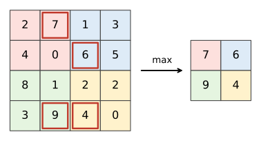
Filling the gap 10.8: what pooling buys, exactly and approximately pp. 296–298
The book says pooling gives "some degree of local translation invariance". Here is what can be proved, and what is only approximate.
Derivation
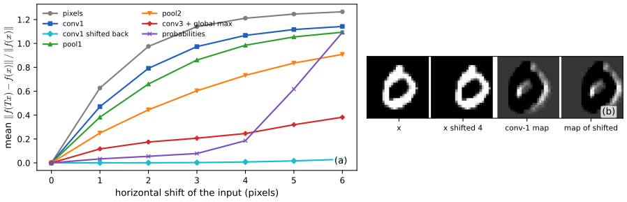
(a) Global pooling gives exact invariance. Let \(f\) be an equivariant stack of convolutional layers on a periodic grid (Result 10.1) and \(g_k=\max_{\bm n}f_k(X)_{\bm n}\) or \(g_k\)\({}=\frac1{|\Omega|}\sum_{\bm n}f_k(X)_{\bm n}\). Since \(f(T_{\bm s}X)=T_{\bm s}f(X)\) is a permutation of the positions of \(f(X)\), and the max and the mean are permutation invariant, \(g(T_{\bm s}X)=g(X)\) for every shift. Our network ends with exactly such a global max over positions, so apart from border effects and from the strides discussed in (b), its output is shift invariant.
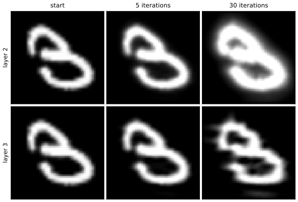
(b) Local pooling with stride \(s\) is equivariant only to shifts by multiples of \(s\): if \(\bm t=s\bm u\), the windows of \(T_{\bm t}F\) are the windows of \(F\) moved by \(\bm u\) whole windows, so the pooled map moves by \(\bm u\). For other shifts the pooled map changes. Two facts limit how much. (i) Max-pooling is 1-Lipschitz in the max norm: \(|\max_{w}F-\max_{w}G|\le\max_{w}|F-G|\) over each window \(w\) (if the maximum of \(F\) is at \(p\), then \(\max F-\max G\le F_p-G_p\), and symmetrically). So a small change of the feature map gives a small change of the pooled map. (ii) If a feature map has an isolated peak and the shift keeps it inside the same window, the max-pooled map does not change at all (checked numerically); average pooling of a peak that stays in its window is likewise unchanged. Neither holds when the peak crosses a window boundary.
(c) Depth. Composing (b) over several layers, a shift by one pixel changes the deeper, coarser maps by less, in relative terms, than the shallower ones, and a final global pooling removes what remains. Figure 10.S1 measures this on our trained network: for a shift by 3 pixels the relative change is 1.14 for the pixels, 0.97 for the layer-1 maps, 0.86 after the first pooling, 0.60 after the second, 0.21 after the global max and 0.08 for the class probabilities, while the layer-1 maps shifted back agree with the maps of the shifted digit to 0.002 (equivariance; the small error comes from the border).
(d) Pooling across channels. If channels \(k=0,\dots,3\) hold filters that are rotated copies of one filter by multiples of \(90^\circ\), \(K_k=R^kK_0\), then rotating the image by \(90^\circ\) permutes these channels cyclically (and rotates each map), because \((RX)\star(RK)=R(X\star K)\) for a rotation \(R\) that maps the grid to itself. The maximum over the four channels (and over positions) is therefore invariant to such rotations. This is the idea behind the book's remark that pooling across channels can learn invariances beyond translation. ∎
10.2.7 Multilayer convolutions
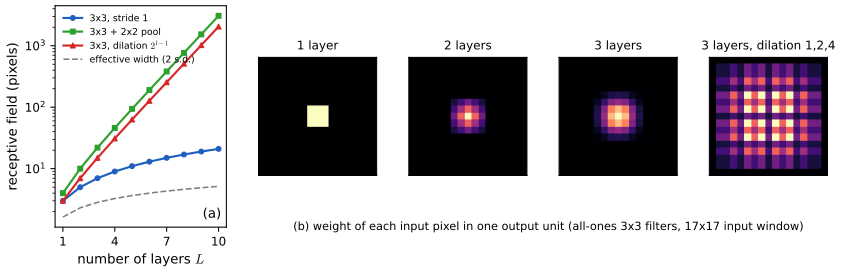
pp. 298–299 Stacking layers lets the network build complex features from simple ones: the \(C_{\rm out}\) channels of one layer are the input channels of the next, and a layer with an \(M\times M\times C_{\rm in}\times C_{\rm out}\) filter tensor has \((M^2C_{\rm in}+1)C_{\rm out}\) parameters. (The book calls the number of channels the "depth" of a feature map only in quotation marks, reserving depth for the number of layers.) Units in later layers depend on ever larger regions of the input (Figure 10.9). For classification, one or two fully connected layers at the end combine information from the whole image; they are affordable because pooling has made the last maps small, though they may still hold most of the parameters.
Result 10.3 (receptive fields) pp. 298–299, 301, Figure 10.9
- For a stack of layers \(l=1,\dots,L\) with filter (or pooling window) size \(k_l\), stride \(s_l\) and dilation \(d_l\), the receptive field \(r_l\) (in input pixels, along one axis) and the jump \(j_l\) (input pixels between neighbouring units of layer \(l\)) satisfy \[r_l=r_{l-1}+d_l(k_l-1)\,j_{l-1},\qquad j_l=j_{l-1}s_l,\qquad r_0=j_0=1.\] Two width-3 layers: 3 units of the middle layer and 5 inputs (Figure 10.9). Our network: 5, 6, 14, 16 and 24 pixels after conv 1, pool 1, conv 2, pool 2 and conv 3.
- Stride-1 layers of \(3\times3\) filters: \(r_L=2L+1\). Two such layers see \(5\times5\) with \(2\cdot9C^2\) weights between \(C\)-channel maps, against \(25C^2\) for one \(5\times5\) layer; three see \(7\times7\) with \(27C^2\) against \(49C^2\), and add two extra nonlinearities.
- Effective receptive field. In a linear stack of \(L\) all-ones \(3\times3\) filters the weight of input pixel \(\bm p\) in the centre output is the \(L\)-fold convolution of a \(3\times3\) box, a product of two discrete distributions with variance \(2L/3\) per axis. The theoretical width \(2L+1\) grows linearly in \(L\), but the standard deviation of the weights only like \(\sqrt{2L/3}\): most of the influence comes from a central region whose size grows like \(\sqrt L\) (Luo et al., 2016).
Proof
(1) By induction. A unit of layer \(l-1\) sees \(r_{l-1}\) input pixels, and neighbouring units of layer \(l-1\) are \(j_{l-1}\) input pixels apart. A unit of layer \(l\) combines \(k_l\) units of layer \(l-1\) spaced \(d_l\) apart, whose leftmost and rightmost are \(d_l(k_l-1)\) units, i.e. \(d_l(k_l-1)j_{l-1}\) input pixels, apart; the union of their receptive fields is an interval of length \(r_{l-1}+d_l(k_l-1)j_{l-1}\) (contiguous, since for \(d_l\,j_{l-1}\le r_{l-1}\) neighbouring fields overlap or touch, which holds in all the stacks here). Moving one unit along layer \(l\) moves \(s_l\) units along layer \(l-1\), so \(j_l=s_lj_{l-1}\). Our network: conv 5 (\(r=5,j=1\)); pool 2/2 (\(6,2\)); conv 5 (\(6+4\cdot2=14\)); pool 2/2 (\(14+2=16,4\)); conv 3 (\(16+2\cdot4=24\)). A numerical test compares the recursion with the support of the input gradient computed by automatic differentiation for five stacks.
(2) With \(k=3,s=d=1\): \(r_L=1+2L\). Weight counts: a layer from \(C\) to \(C\) channels with an \(M\times M\) filter has \(M^2C^2\) weights.
(3) Without nonlinearities the stack is one convolution with the kernel \(K^{*L}\) (Filling the gap 10.3), and the gradient of the centre output with respect to the input is that kernel, flipped. For the all-ones \(3\times3\) kernel, \(K=u\,u^\T\) with \(u=(1,1,1)\), so \(K^{*L}=u^{*L}(u^{*L})^\T\) and each axis is the \(L\)-fold convolution of the uniform distribution on \(\{-1,0,1\}\) (up to normalisation), the distribution of a sum of \(L\) independent such variables: mean 0, variance \(L\cdot\frac23\). By the central limit theorem the profile approaches a Gaussian of standard deviation \(\sqrt{2L/3}\); the fraction of the total weight outside \(\pm c\sqrt{2L/3}\) tends to \(2(1-\Phi(c))\), however large the nominal width \(2L+1\). A numerical test confirms variance exactly 4 for \(L=6\). With random weights and nonlinearities the picture is similar on average (Luo et al., 2016). ∎
p. 299 A complete CNN interleaves convolutions with pooling and ends with fully connected layers. The number of layers, channels, filter sizes and strides are hyperparameters, and because each training run is expensive they are hard to compare systematically on validation data.
10.2.8 Example network architectures
pp. 299–301 CNNs were the first deep networks (more than two learnable layers) to be deployed: LeNet read handwritten digits (LeCun et al., 1989, 1998). ImageNet (Deng et al., 2009), with about 14 million images in nearly 22,000 categories, and its 1,000-class challenge (1.28 million training images; top-1 and top-5 error) drove the progress: random guessing has top-1 error 99.9%; early methods reached a top-5 error of about 25.5%; AlexNet (Krizhevsky, Sutskever and Hinton, 2012), with ReLUs, GPUs and dropout, 15.3%; later networks about 3%, below the roughly 5% of humans on this task (Dodge and Karam, 2017).
VGG-16 (Simonyan and Zisserman, 2014) has a deliberately uniform design (Figure 10.10, a diagram, here computed): a \(224\times224\times3\) input; thirteen \(3\times3\) convolutional layers with stride 1, same padding and ReLU, in five blocks of 2, 2, 3, 3 and 3 layers with 64, 128, 256, 512 and 512 channels; a \(2\times2\) max-pooling with stride 2 after each block (\(224\to112\to56\to28\to14\to7\)); then fully connected layers of 4,096, 4,096 and 1,000 units with a softmax output. Each down-sampling quarters the number of positions and the following block doubles the channels, so the representation shrinks gradually. About 138 million parameters, nearly 103 million of them in the first fully connected layer (Exercise 10.8).
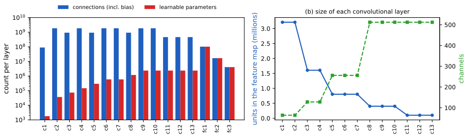
Erratum. p. 301 The book says that "most of the connections are in the first convolutional layer". With connections counted as in Exercise 10.8, the first layer has the fewest among the convolutional layers (89.9 million: it has only 3 input channels); layers c2, c4, c6, c7, c9 and c10 each have about 1.85 billion, and the 13 convolutional layers together hold 99.2% of all connections. The statement is right if read as "in the convolutional layers".
p. 301 AlexNet used \(11\times11\) filters with stride 4. Stacking small filters reaches the same receptive field with fewer parameters (Result 10.3), an inductive bias: the large filter must factor through small ones. Training needs only the network function to be coded, since automatic differentiation (Section 8.2 of the book) computes the derivatives. The next result shows what it computes for a convolutional layer.
Result 10.4 (the backward pass of a convolutional layer) p. 301 (and Section 8.1)
For the layer of Definition 10.2 with error \(E\) and \(\delta_{o,j,k}\)\({}=\partial E/\partial a_{o,j,k}\):
- Bias and weights: \[\frac{\partial E}{\partial b_o}=\sum_{j,k}\delta_{o,j,k},\qquad \frac{\partial E}{\partial W_{o,c,l,m}}=\sum_{j,k}\delta_{o,j,k}\,X^{\rm pad}_{c,\,jS+lD,\,kS+mD},\] the cross-correlation of the (padded) input channel \(c\) with the error map \(\delta_o\) (dilated by \(S\) when \(S>1\)). The sum over \((j,k)\) is the rule for shared weights: add the derivatives of all the connections that share the weight.
- Input (for \(S=D=1\)): \[\frac{\partial E}{\partial X^{\rm pad}_{c,u,v}}=\sum_o\sum_{l,m}W_{o,c,l,m}\,\delta_{o,\,u-l,\,v-m},\] the 'full' convolution (10.19) of the error maps with the kernels, equivalently the cross-correlation of the zero-padded (by \(M-1\)) error maps with the kernels rotated by \(180^\circ\) and with the roles of input and output channels swapped; then remove the padding \(P\). For stride \(S>1\) it is a transposed convolution with stride \(S\) (Section 10.5.3): insert \(S-1\) zeros between neighbouring \(\delta\)'s and proceed as for \(S=1\).
The backward pass costs the same order of operations as the forward pass, and the backpropagation through max-pooling routes each \(\delta\) to the input that won the maximum (the max-unpooling of Section 10.5.2), through average pooling it spreads \(\delta/k^2\) over the window.
Proof
\(a_{o,j,k}\) depends on \(b_o\) with derivative 1, on \(W_{o,c,l,m}\) with derivative \(X^{\rm pad}_{c,jS+lD,kS+mD}\), and on \(X^{\rm pad}_{c,u,v}\) through every term with \(jS+lD=u\), \(kS+mD=v\). The chain rule, \(\partial E/\partial\theta\)\({}=\sum_{o,j,k}\delta_{o,j,k}\,\partial a_{o,j,k}/\partial\theta\), gives (1) at once. For the input, \[\frac{\partial E}{\partial X^{\rm pad}_{c,u,v}}=\sum_o\sum_{\substack{j,k,l,m:\\ jS+lD=u,\ kS+mD=v}}W_{o,c,l,m}\,\delta_{o,j,k}.\] With \(S=D=1\), \(j=u-l\) and \(k=v-m\), which is (2), with \(\delta\) taken as 0 outside its range; this is the 'full' convolution of \(\delta_o\) with \(W_{o,c}\). By Filling the gap 10.3 it equals the cross-correlation of \(\delta_o\), padded by \(M-1\), with the flipped kernel \(W_{o,c,M-1-l,M-1-m}\), summed over \(o\): a convolutional layer from \(C_{\rm out}\) to \(C\) channels with the transposed and flipped filter tensor. For \(S>1\), the condition \(jS+l=u\) says that the \(\delta\)'s sit on a grid of spacing \(S\) in input coordinates, i.e. the operation is the transposed convolution of Result 10.9. In matrix form all of this is the statement that the backward pass multiplies by \(\bA^\T\), the transpose of the sparse matrix of Filling the gap 10.4. Numerical tests compare all three gradients with PyTorch's automatic differentiation (stride 2, padding 1, dilation 2), the weight gradient with finite differences, the stride-1 input gradient with the flipped-kernel convolution, and the stride-2 input gradient with PyTorch's conv_transpose2d. Pooling: max-pooling is locally the selection of one input per window, whose derivative is 1 for the winner and 0 for the rest; average pooling has derivative \(1/k^2\) for each input of the window. ∎
See also the companion course: backpropagation in Section 5.3.1 and tied weights in Filling the gap 5.5.
Separable filters. A filter that factorises, \(K(l,m)=F(l)G(m)\), can be applied as a one-dimensional convolution along rows followed by one along columns, at a cost of about \(JK(L+M)\) instead of \(JKLM\) operations (Exercise 10.9); the Gaussian filter of the convolution demo is an example. Learned filters are not separable in general, and imposing it restricts the model.
10.3 Visualizing Trained CNNs
p. 302 What do the units of a trained CNN detect? The answers show a striking resemblance to the mammalian visual system, and they also expose weaknesses.
10.3.1 Visual cortex
pp. 302–303 Hubel and Wiesel (1959) recorded single neurons in the visual cortex of cats. "Simple cells" respond to an edge at a particular orientation and position; their responses are well modelled by Gabor filters
\[ G(x,y)=A\exp\!\big(-\alpha\tilde x^2-\beta\tilde y^2\big)\sin(\omega\tilde x+\varphi) \tag{10.6} \]with rotated coordinates
\[ \tilde x=(x-x_0)\cos\theta+(y-y_0)\sin\theta, \tag{10.7} \] \[ \tilde y=-(x-x_0)\sin\theta+(y-y_0)\cos\theta. \tag{10.8} \]"Complex cells" combine simple cells and tolerate small shifts, like pooling units; deeper areas respond to ever more specific and invariant stimuli ("grandmother cells"). These findings inspired the neocognitron (Fukushima, 1980): local receptive fields, shared weights and pooling, but trained greedily layer by layer, before backpropagation.
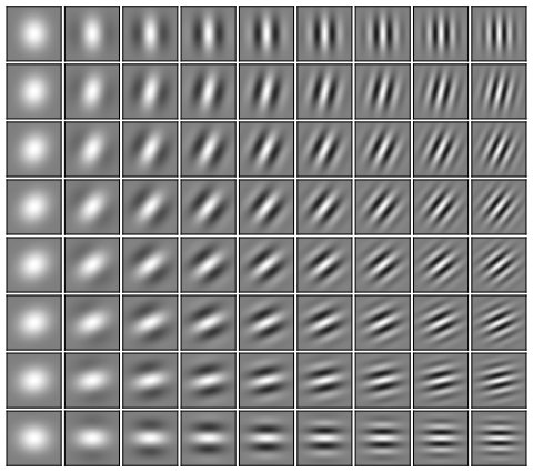
Filling the gap 10.9: a Gabor filter is tuned to one orientation and one frequency p. 302, (10.6)–(10.8)
The book describes (10.6) as an oriented sinusoid under a decaying envelope. Its Fourier transform makes the tuning precise.
Derivation
Rotation. (10.7)–(10.8) are \((\tilde x,\tilde y)^\T\)\({}=\bm R_\theta^\T(x-x_0,y-y_0)^\T\) with \(\bm R_\theta\) the rotation by \(\theta\); since \(\bm R_\theta\) is orthogonal, \(\tilde x^2+\tilde y^2=(x-x_0)^2+(y-y_0)^2\), and the filter at angle \(\theta\) is the \(\theta=0\) filter rotated by \(\theta\) about \((x_0,y_0)\) (checked numerically).
Spectrum. Take \(x_0=y_0=0\), \(\theta=0\) first. With \(\sin(\omega x+\varphi)\)\({}=\frac1{2i}(e^{i(\omega x+\varphi)}-e^{-i(\omega x+\varphi)})\) and the Gaussian integral \(\int e^{-\alpha x^2-i\xi x}\d x\)\({}=\sqrt{\pi/\alpha}\,e^{-\xi^2/(4\alpha)}\), the transform \(\widehat G(\xi_1,\xi_2)\)\({}=\iint G(x,y)e^{-i(\xi_1x+\xi_2y)}\d x\,\d y\) is \[ \widehat G(\bm\xi)=\frac{A\pi}{2i\sqrt{\alpha\beta}}\Big(e^{i\varphi}e^{-\frac{(\xi_1-\omega)^2}{4\alpha}-\frac{\xi_2^2}{4\beta}}-e^{-i\varphi}e^{-\frac{(\xi_1+\omega)^2}{4\alpha}-\frac{\xi_2^2}{4\beta}}\Big): \] two Gaussian bumps centred at \(\pm(\omega,0)\) with widths \(\sqrt{2\alpha}\) and \(\sqrt{2\beta}\). Rotating the filter rotates its transform by the same angle, so in general the bumps sit at \(\pm\omega(\cos\theta,\sin\theta)\). A Gabor filter is therefore a band-pass filter: its response \(\sum G\,I\) to an image (an inner product, Parseval) picks out the image's content near spatial frequency \(\omega\) in direction \(\theta\); a large envelope (small \(\alpha,\beta\)) gives sharp tuning in frequency but poor localisation in space, and vice versa (the uncertainty principle: the product of the spatial and frequency widths of a Gaussian is fixed). A numerical test finds the peak of the discrete spectrum at \(|\bm k|=2.83\) and angle 0.59 for \(\omega=3\), \(\theta=0.6\) (one frequency bin is 0.39). ∎
10.3.2 Visualizing trained filters
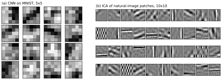
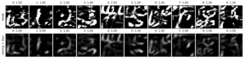
pp. 303–304 First-layer filters act on image patches, so they can be displayed directly; a unit responds strongly when the inner product of its filter with the patch is large (Filling the gap 10.2). The first-layer filters of AlexNet on ImageNet look strikingly like Gabor filters. This does not make CNNs models of the brain: many statistical methods applied to natural images give such filters (Hyvärinen, Hurri and Hoyer, 2009), because they reflect the statistics of natural images. Figure 10.12 shows both sides at small scale.
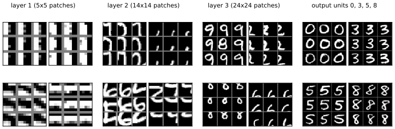
pp. 303–304 Deeper units see groups of filter responses, not pixels. One way to see what they detect, in the spirit of Hubel and Wiesel, is to show the network many images and keep the patches (the unit's receptive field) that activate the unit most. Zeiler and Fergus (2013) found edges in layer 1, textures and simple shapes in layer 2, object parts in layer 3 and whole objects in layer 5 of a five-layer ImageNet network.
p. 304 Instead of searching a data set, one can optimise the input to maximise a unit's activation (Zeiler and Fergus, 2013; Simonyan, Vedaldi and Zisserman, 2013; Yosinski et al., 2015). For an output unit it is better to maximise the pre-activation \(a^{(c)}\) that feeds the softmax than the probability \(y_c\).
Filling the gap 10.10: why maximise the pre-softmax output and not the probability p. 304
Derivation
With \(y_c=e^{a^{(c)}}/\sum_je^{a^{(j)}}\), \(\ln y_c=a^{(c)}-\ln\sum_je^{a^{(j)}}\), and differentiating with respect to the image \(\bx\), \[ \nabla_\bx\ln y_c=\nabla_\bx a^{(c)}-\sum_jy_j\nabla_\bx a^{(j)}=(1-y_c)\nabla_\bx a^{(c)}-\sum_{j\ne c}y_j\nabla_\bx a^{(j)} \] (the derivative of log-sum-exp is the softmax; see Section 4.3.4 of the companion course). Ascending \(\ln y_c\) therefore also pushes down every other class in proportion to its probability: the image can become "more dog" by becoming "less cat", without becoming any more dog-like. Ascending \(a^{(c)}\) involves class \(c\) alone. Moreover, once \(y_c\approx1\) the first term is multiplied by \(1-y_c\approx0\) and the probability gives almost no signal, while \(a^{(c)}\) keeps growing. A numerical test confirms the identity against automatic differentiation on our network.
Regularisation. \(a^{(c)}\) is unbounded in \(\bx\) (for a ReLU network it is piecewise linear, so along a ray it eventually grows linearly), and unconstrained ascent drives pixels to large values with high-frequency patterns. Hence the objective \(a^{(c)}(\bx)-\lambda\|\bx\|^2\), which is bounded above whenever \(a^{(c)}\) grows at most linearly, plus heuristics: periodic blurring (removing high frequencies) and clipping to the valid pixel range, as in Yosinski et al. (2015). ∎
10.3.3 Saliency maps
See also the companion course, Section 5.3.4 (the Jacobian of the outputs with respect to the inputs, the simplest saliency map).
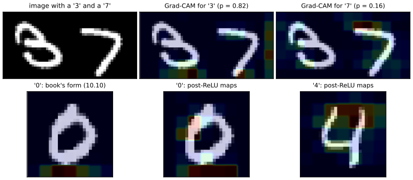
p. 305 A saliency map shows which regions of an image matter most for the label. The last convolutional layer is the natural place to look: it still has spatial resolution, and its features are the most semantic. Grad-CAM (Selvaraju et al., 2016) averages, over the positions of channel \(k\) of that layer, the derivatives of the pre-softmax output for class \(c\) with respect to the pre-activations,
\[ \alpha_k=\frac1{M_k}\sum_i\sum_j\frac{\partial a^{(c)}}{\partial a^{(k)}_{ij}}, \tag{10.9} \]with \(M_k\) the number of positions in channel \(k\), and forms the weighted sum of the channel maps
\[ L=\sum_k\alpha_kA^{(k)}, \tag{10.10} \]with \(A^{(k)}\) the matrix of the \(a^{(k)}_{ij}\). \(L\) has the size of the last convolutional map (\(14\times14\) for VGG-16, \(7\times7\) for our network) and is up-sampled and overlaid on the image as a heat map.
Algorithm 10.1 (Grad-CAM) p. 305, (10.9)–(10.10)
- Forward-propagate the image; keep the maps \(A^{(k)}\) of the last convolutional layer.
- Backpropagate from the pre-softmax output \(a^{(c)}\) (not from \(y_c\); Filling the gap 10.10) to that layer, giving \(\partial a^{(c)}/\partial a^{(k)}_{ij}\).
- Average over positions to get \(\alpha_k\) (10.9); form \(L=\sum_k\alpha_kA^{(k)}\) (10.10).
- Keep the positive part \(\max(L,0)\), up-sample to the image size and overlay.
The book takes \(A^{(k)}\) to be pre-activations. Selvaraju et al. use the activations after the ReLU (and the derivatives with respect to them) and apply a ReLU to \(L\). The difference matters: with pre-activations, a channel with a negative weight \(\alpha_k\) and a negative pre-activation contributes positively, so empty background can light up. Both forms are in the feature-map demo.
Result 10.5 (Grad-CAM decomposes the class score for a global pooling head) p. 305
Let the last convolutional layer have post-ReLU maps \(Z^{(k)}\), \(k=1,\dots,K\), with \(M\) positions each, followed by global pooling and a linear output \(a^{(c)}=\sum_kw_{ck}g_k+b_c\).
- Average pooling, \(g_k=\frac1M\sum_{ij}Z^{(k)}_{ij}\): Grad-CAM on the post-ReLU maps has \(\alpha_k=w_{ck}/M\) and \[\sum_{i,j}L_{ij}=a^{(c)}-b_c,\qquad L=\sum_k\frac{w_{ck}}{M}Z^{(k)}:\] the heat map is an exact decomposition of the class score over positions (the class activation map of Zhou et al., 2016).
- Max pooling, \(g_k=\max_{ij}Z^{(k)}_{ij}\), as in our network: \(a^{(c)}-b_c=\sum_kw_{ck}Z^{(k)}_{\bm p_k}\) with \(\bm p_k\) the position of channel \(k\)'s maximum, so the score is a sum of at most \(K\) point contributions, and the gradient \(\partial a^{(c)}/\partial Z^{(k)}\) is \(w_{ck}\) at \(\bm p_k\) and 0 elsewhere; (10.9) spreads it uniformly, \(\alpha_k=w_{ck}/M\).
Proof
(1) \(\partial a^{(c)}/\partial Z^{(k)}_{ij}\)\({}=w_{ck}\,\partial g_k/\partial Z^{(k)}_{ij}\)\({}=w_{ck}/M\) for every position, so the average (10.9) is \(w_{ck}/M\), and \(\sum_{ij}L_{ij}\)\({}=\sum_kw_{ck}\frac1M\sum_{ij}Z^{(k)}_{ij}\)\({}=\sum_kw_{ck}g_k\)\({}=a^{(c)}-b_c\). (2) \(g_k\) depends only on the maximising entry (almost everywhere, i.e. without ties), with derivative 1, which gives both statements. Numerical tests confirm (1) on random maps and (2) on our network, where the gradient on the last layer has at most 32 non-zero entries. In general (a nonlinear head) Grad-CAM is only a first-order, gradient-weighted summary and has no such exact reading. ∎
10.3.4 Adversarial attacks
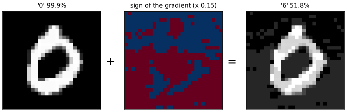
pp. 306–307 Gradients with respect to the pixels also produce adversarial examples (Szegedy et al., 2013): changes too small to see that make the network misclassify. The fast gradient sign method (Goodfellow, Shlens and Szegedy, 2014) moves every pixel by \(\pm\epsilon\):
\[ \bx'=\bx+\epsilon\,\sign\!\big(\nabla_\bx E(\bx,t)\big), \tag{10.11} \]with \(t\) the true label and \(E\) for example the negative log likelihood; training lowers \(E\) by changing the weights, the attack raises it by changing the image. The images can be misclassified with high confidence (a panda becomes a gibbon in Figure 10.16 of the book).
Algorithm 10.2 (fast gradient sign method, and its iterative and targeted versions) p. 306, (10.11)
- Compute \(\bg=\nabla_\bx E(\bx,t)\) by backpropagation to the input (for the cross-entropy, start from \(\partial E/\partial\ba=\by-\bt\)).
- Set \(\bx'\)\({}=\operatorname{clip}_{[0,1]}(\bx+\epsilon\,\sign\bg)\).
- Iterative: repeat steps 1–2 \(n\) times with step \(\epsilon/n\), each time projecting back onto \(\{\|\bx'-\bx\|_\infty\le\epsilon\}\) and \([0,1]\). Targeted: use \(-\nabla_\bx E(\bx,c)\) for a chosen class \(c\).
Result 10.6 (the sign step is the best first-order attack, and the linear explanation) pp. 306–307
- To first order, \(E(\bx+\bdelta)\approx E(\bx)+\bg^\T\bdelta\). Over all perturbations with \(\|\bdelta\|_\infty\le\epsilon\) (no pixel changes by more than \(\epsilon\)), \[\max_{\|\bdelta\|_\infty\le\epsilon}\bg^\T\bdelta=\epsilon\|\bg\|_1,\] attained at \(\bdelta=\epsilon\sign\bg\): (10.11) is the optimal step for the linearised error. (Under \(\|\bdelta\|_2\le\epsilon\) the optimum is \(\epsilon\bg/\|\bg\|_2\), with gain \(\epsilon\|\bg\|_2\).)
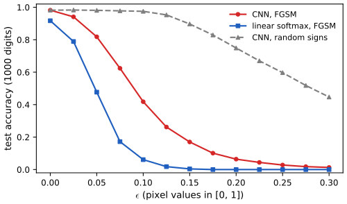
- For a random sign perturbation \(\bdelta=\epsilon\bm r\), \(r_i=\pm1\) independently with probability \(\frac12\), the first-order change has mean 0 and standard deviation \(\epsilon\|\bg\|_2\). Since \(\|\bg\|_2\le\|\bg\|_1\le\sqrt D\|\bg\|_2\), the adversarial direction beats a typical random one by the factor \(\|\bg\|_1/\|\bg\|_2\), which is of order \(\sqrt D\) when the gradient is spread over many of the \(D\) pixels.
- Hence even a linear model \(a=\bw^\T\bx\) is fragile in high dimension: a per-pixel change of \(\epsilon\) can shift \(a\) by \(\epsilon\|\bw\|_1\)\({}\approx\epsilon D\,\overline{|w|}\), which grows with \(D\) while the perceptibility of the change, \(\|\bdelta\|_\infty=\epsilon\), does not.
Proof
(1) Hölder's inequality: \(\bg^\T\bdelta\)\({}=\sum_ig_i\delta_i\)\({}\le\sum_i|g_i||\delta_i|\)\({}\le\epsilon\sum_i|g_i|\), with equality when \(\delta_i=\epsilon\sign g_i\) (any value when \(g_i=0\)). For the 2-norm, Cauchy–Schwarz gives \(\bg^\T\bdelta\le\|\bg\|_2\epsilon\), with equality at \(\bdelta=\epsilon\bg/\|\bg\|_2\). (2) \(\E[\bg^\T\bm r]=0\) and \(\var[\bg^\T\bm r]\)\({}=\sum_ig_i^2\var[r_i]\)\({}=\|\bg\|_2^2\). The norm inequalities: \(\|\bg\|_1^2\)\({}=\sum_{i,j}|g_i||g_j|\)\({}\ge\sum_ig_i^2\), and Cauchy–Schwarz with the all-ones vector gives \(\|\bg\|_1\le\sqrt D\|\bg\|_2\). (3) Apply (1) with \(\bg=\bw\). On MNIST (\(D=784\), \(\sqrt D=28\)) the weight difference between two classes of our linear softmax model has \(\|\bw\|_1/\|\bw\|_2=19.4\): the sign step moves the logit difference about 19 times further than random signs of the same size. Deep networks are fragile for the same reason, being close to piecewise linear (ReLU) and so, locally, linear models in many dimensions (Goodfellow, Shlens and Szegedy, 2014). This also explains why the same perturbation often transfers between models: it follows the sign of gradients that different models trained on the same data tend to share. ∎
p. 307 Adversarial images transfer between networks, and physical objects can be altered so that ordinary photographs of them are misread (stop signs read as speed-limit signs; Figure 10.17, photographs, Eykholt et al., 2018). Simple attacks can be countered by changing the training (for example by training on adversarial examples), but stronger attacks remain hard to defeat; this is an open research area.
10.3.5 Synthetic images
p. 308 DeepDream (Mordvintsev, Olah and Tyka, 2015) exaggerates whatever a chosen layer sees in an image: forward-propagate the image to the layer, set the backpropagation variables \(\delta\) of that layer equal to its pre-activations, backpropagate to the pixels and take a small step along the result. This is gradient ascent on
\[ F(I)=\sum_{i,j,k}a_{ijk}(I)^2, \tag{10.12} \]with \(a_{ijk}(I)\) the pre-activation at row \(i\), column \(j\), channel \(k\) of the layer for input image \(I\), with spatial smoothing and pixel clipping as regularisers. Starting from noise gives images generated entirely by the network; mostly the method makes art.
Filling the gap 10.11: DeepDream is gradient ascent on (10.12) p. 308; Exercise 10.10
Derivation
Backpropagation computes \(\partial F/\partial I\) by starting from \(\delta_{ijk}=\partial F/\partial a_{ijk}\) at the chosen layer and applying the chain rule layer by layer down to the pixels (Section 8.1 of the book; for convolutional layers this is Result 10.4). For (10.12), \(\partial F/\partial a_{ijk}=2a_{ijk}\). Since every backward step is linear in the \(\delta\)'s, starting from \(\delta=a\) instead gives exactly \(\frac12\nabla_IF\), a positive multiple of the gradient: a step along it is a gradient-ascent step on \(F\) with half the learning rate. (The units of later layers are irrelevant: \(F\) does not depend on them.) A numerical test confirms on our network that backpropagating \(\delta=2a\) from layer 2 gives the autograd gradient of \(\sum a^2\). Squaring rewards large responses of either sign; with ReLU units one may prefer \(\sum\ReLU(a)^2\), which amplifies only the features that are present. ∎
10.4 Object Detection
pp. 308–309 ImageNet images are dominated by one object, so classifying the whole image makes sense. Many applications need more, and the representations learned by a CNN on a large data set transfer well (Section 6.3.4, transfer learning, and the skin-lesion example of Section 1.1.1), so a pre-trained CNN can be fine-tuned for detection, segmentation and other tasks.
10.4.1 Bounding boxes
pp. 309–310 A detector must say which objects are present and where. The location is described by a bounding box, the tightest rectangle around the object, \(\bb=(b_x,b_y,b_W,b_H)\): centre, width and height, in pixels or as fractions with the top-left corner of the image at \((0,0)\) and the bottom-right at \((1,1)\) (Figure 10.19, a photograph). If an image contains exactly one object from \(C\) classes, the network has \(C\) softmax outputs for the class (Section 5.3 of the book; Section 5.4.4 in these notes) and four linear outputs for the box, trained with a sum-of-squares error, i.e. a Gaussian likelihood for the coordinates (Section 4.1.2). YOLO (Redmon et al., 2015) divides the image into a \(7\times7\) grid and predicts, for each cell, the class and box of an object centred in it, from features of the whole image.
Background. When a window may contain no object, the outputs need a "background" option. Exercise 10.11 compares a softmax over \(C+1\) classes with a factorised output (an object-presence probability times a distribution over the \(C\) classes); by the product rule they correspond through \(p(\text{class }i)\)\({}=p(\text{object})\,p(\text{class }i\given\text{object})\) and \(p(\text{background})=1-p(\text{object})\). Our network uses the first option, with digits shifted out of the window as the background examples.
10.4.2 Intersection-over-union
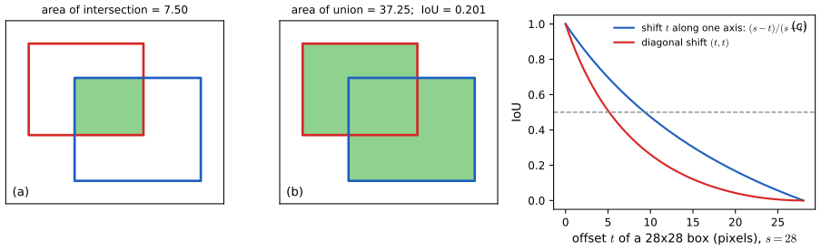
pp. 310–311 To score a predicted box against a ground-truth box, the area of overlap alone is not enough: it depends on the object's size, and it does not penalise a prediction that spills outside the true box. The ratio of the intersection to the union does both.
Definition 10.3 (intersection-over-union) pp. 310–311, Figure 10.20
For two boxes (or any two regions of finite area) \(A\) and \(B\), \[\IoU(A,B)=\frac{|A\cap B|}{|A\cup B|},\] with \(|\cdot|\) the area. A prediction is usually counted as correct if \(\IoU>0.5\).
Result 10.7 (properties of IoU) p. 311
- \(0\le\IoU\le1\); \(\IoU(A,B)=1\) iff \(A=B\) (up to sets of zero area); \(\IoU=0\) iff the boxes do not overlap (in area); IoU is symmetric and unchanged when both boxes are scaled by the same factor or translated together.
- Two \(s\times s\) boxes offset by \(t\le s\) along one axis have \(\IoU=(s-t)/(s+t)\), so \(\IoU>0.5\) iff \(t<s/3\); offset by \((t,t)\), \(\IoU=(s-t)^2/(2s^2-(s-t)^2)\).
- \(d(A,B)=1-\IoU(A,B)\) (the Jaccard distance) is a metric: it satisfies the triangle inequality \(d(A,C)\le d(A,B)+d(B,C)\).
- For disjoint boxes, IoU is 0 in a whole neighbourhood of the prediction, so its gradient is 0: it gives no training signal for a prediction that misses, which is one reason it is used for evaluation rather than as a loss.
Proof
(1) \(A\cap B\subseteq A\cup B\) gives the bounds; \(|A\cap B|=|A\cup B|\) means \(|A\setminus B|+|B\setminus A|=0\). Scaling all lengths by \(\lambda\) multiplies both areas by \(\lambda^2\).
(2) The intersection is \((s-t)\times s\) and the union \(2s^2-(s-t)s\), so \(\IoU=(s-t)/(2s-(s-t))\)\({}=(s-t)/(s+t)\), and \((s-t)/(s+t)>\frac12\iff s>3t\). The diagonal case has intersection \((s-t)^2\).
(3) Write \(d(A,B)=|A\triangle B|/|A\cup B|\) (the symmetric difference, since \(|A\cup B|-|A\cap B|=|A\triangle B|\)). Split \(U=A\cup B\cup C\) into the seven disjoint pieces according to membership of \(A,B,C\). Counting how often each piece appears gives the identity \[|A\triangle B|+|B\triangle C|=|A\triangle C|+2\,|B\setminus(A\cup C)|+2\,|(A\cap C)\setminus B|.\] (For example, points in \(A\) only appear once on each side; points in \(B\) only appear twice on the left and not at all in \(A\triangle C\).) Now, as \(A\cup B\subseteq U\) and \(B\cup C\subseteq U\), \[ d(A,B)+d(B,C)\ge\frac{|A\triangle B|+|B\triangle C|}{|U|}\ge\frac{|A\triangle C|+n}{|A\cup C|+n},\qquad n=|B\setminus(A\cup C)|, \] using the identity (dropping the non-negative \(2|(A\cap C)\setminus B|\) and one copy of \(n\)) and \(|U|=|A\cup C|+n\). Finally \(\frac{p+n}{q+n}\ge\frac pq\) whenever \(0\le p\le q\) and \(n\ge0\) (cross-multiply: \(q(p+n)-p(q+n)=n(q-p)\ge0\)); with \(p=|A\triangle C|\le q=|A\cup C|\) this is \(d(A,C)\). (If \(A\cup C\) has zero area, \(d(A,C)=0\) and there is nothing to prove.) A numerical test verifies the inequality on all 4,060 triples of 30 random boxes.
(4) If the boxes are a positive distance apart, small changes of the prediction keep them disjoint, so IoU stays 0 (checked by finite differences). Losses built on IoU therefore add terms that act when boxes do not overlap (for example the distance between centres), or train the coordinates by sum-of-squares as above. ∎
10.4.3 Sliding windows
pp. 311–313 A simple detector: train a classifier on tightly cropped objects plus a background class, then scan a window over the new image and classify each position; a confident detection gives a box. Scanning at every position, and at several scales, is expensive, and a coarser stride trades location accuracy for speed. But a CNN already slides its filters over the image, so the computations for overlapping windows are shared (Figure 10.21, a diagram), and the scanning can be done by the convolutional network itself (Sermanet et al., 2013). The book's example (Figures 10.22–10.23, diagrams): a \(6\times6\) input, a \(3\times3\) convolution, \(2\times2\) max-pooling and a fully connected output, which can be read as a \(2\times2\) convolution with a single position. Applied to an \(8\times8\) image the same layers give a \(6\times6\) convolutional map, a \(3\times3\) pooled map and a \(2\times2\) array of outputs with shared weights.
Erratum. p. 312 The pooling layer of Figure 10.22 is described as having "non-overlapping receptive fields of size \(2\times2\) with stride 1". Non-overlapping \(2\times2\) windows have stride 2, and only stride 2 gives the stated sizes (\(4\times4\to2\times2\) for the \(6\times6\) input, \(6\times6\to3\times3\) for the \(8\times8\) one; stride 1 would give \(3\times3\) and \(5\times5\)).
Result 10.8 (sliding windows are a convolution) pp. 311–313; Exercise 10.12
Let a network consist of valid convolutions and poolings with strides \(s_1,\dots,s_L\), whose last layer has a single output position for an input window of size \(w\) (a fully connected layer written as a convolution). Applied to a larger image, the same layers produce an array of outputs, and the output at position \((u,v)\) equals the network applied to the window whose top-left corner is \((Su,Sv)\), with \(S=s_1s_2\cdots s_L\). Window positions that are not multiples of \(S\) are not evaluated. For the network of Figures 10.22–10.23, \(S=1\cdot2\cdot1=2\): the four outputs on the \(8\times8\) image are the windows at offsets \((0,0),(0,2),(2,0),(2,2)\).
Proof
By induction on the layers, a unit at position \(\bm n\) of layer \(l\) depends only on the input pixels \(J_l\bm n+\{0,\dots,r_l-1\}^2\), with \(J_l=s_1\cdots s_l\) the jump and \(r_l\) the receptive field (Result 10.3), through the same weights at every position (the layers are valid convolutions and poolings, so no padding enters). The final unit at \(\bm n\) therefore computes the same function of the pixels in its \(r_L\times r_L\) field as the final unit at \(\bm0\) does of the pixels in its field. For the small network \(r_L=w\) (one output for a \(w\times w\) window), so output \(\bm n\) is the network applied to the window at \(S\bm n\). Positions in between are skipped because no unit's receptive field starts there. A numerical test confirms both statements with random weights: the four outputs on an \(8\times8\) input equal the network on the four windows at even offsets, and the window at offset \((1,0)\) matches none of them. With 'same' padding (as in our MNIST network) the identity fails near the window borders, because zeros inside a window are replaced by real neighbouring pixels; we therefore scan our network window by window. ∎
Exercise 10.12 counts the savings: 291 operations for one \(6\times6\) pass and 667 for the \(8\times8\) network, against 1,164 for the four windows it actually evaluates (a factor 1.75) or 2,619 for all nine stride-1 windows (a factor 3.9, but five of those windows are not computed by the big network). For large images and deep networks the shared part dominates and the factor becomes large.
10.4.4 Detection across scales
pp. 313–314 Objects come in different sizes and aspect ratios (a cat sitting or lying). Instead of windows of many shapes, keep one window and scan copies of the image rescaled by several pairs of factors \((\lambda_x,\lambda_y)\) (Figure 10.24, photographs). A detection with box \((b_x,b_y,b_W,b_H)\) in a copy scaled by \((\lambda_x,\lambda_y)\) corresponds in the original to \[(b_x/\lambda_x,\ b_y/\lambda_y,\ b_W/\lambda_x,\ b_H/\lambda_y):\] the map \((x,y)\mapsto(\lambda_xx,\lambda_yy)\) is linear, so its inverse maps the centre to the centre and divides the side lengths by the factors. A fixed square window thus detects boxes of every aspect ratio \(\lambda_y/\lambda_x\) used.
10.4.5 Non-max suppression
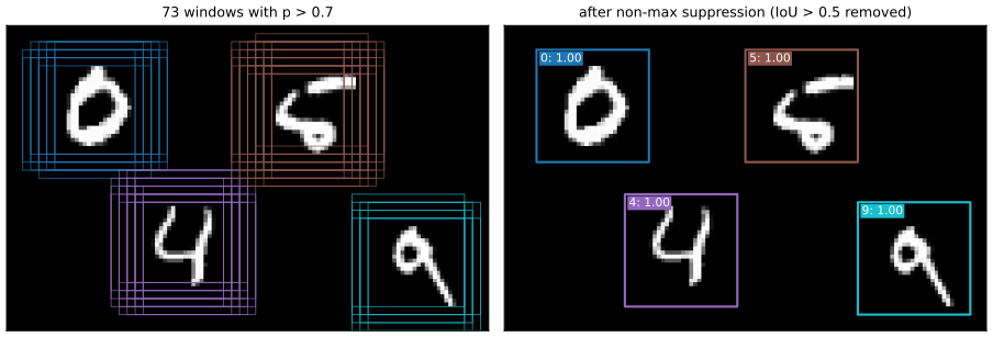
pp. 314–315 A scanning detector fires at many neighbouring positions on the same object (Figure 10.25). Non-max suppression keeps one detection per object, class by class:
Algorithm 10.3 (non-max suppression, for one class) p. 314
- Scan the image and compute the probability of the class at every window position.
- Discard all boxes with probability below a threshold, say 0.7.
- While boxes remain: declare the most probable remaining box a detection, and discard every remaining box whose IoU with it exceeds a threshold, say 0.5.
The kept boxes overlap pairwise by IoU at most 0.5 (each kept box survived the comparison with every earlier one). The loop costs \(O(n^2)\) IoU evaluations for \(n\) candidates, \(O(n\log n)\) for the sorting.
10.4.6 Fast region CNNs
pp. 314–315 Scanning applies the full network everywhere, even where no object is likely. Region-proposal methods first find promising regions cheaply (for example by segmentation) and run the full network only there: fast R-CNN (Girshick, 2015); a proposal network trained jointly with the detector gives faster R-CNN (Ren et al., 2015). And instead of a fine grid of windows, the network can predict the box relative to the window position (Sermanet et al., 2013), combining sliding windows with the regression outputs of Section 10.4.1.
10.5 Image Segmentation
p. 315 Semantic segmentation assigns every pixel to one of \(C\) classes. The output has the spatial size of the image and \(C\) channels of class probabilities; colouring each pixel by its most probable class gives a segmentation image (Figure 10.26, a photograph).
10.5.1 Convolutional segmentation
pp. 315–316 A patch classifier applied at every pixel would do it, but would repeat the computations of overlapping patches; by Result 10.8 those are shared if the whole network is convolutional, every layer with stride 1, same padding and no pooling, and a per-pixel softmax with shared weights at the end. Such a network keeps full resolution in every layer, which is prohibitively costly for the many channels and layers needed.
10.5.2 Up-sampling
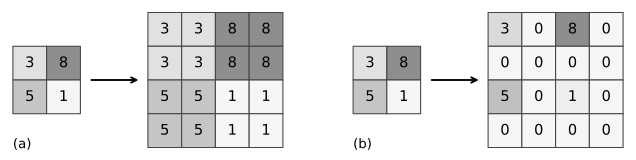
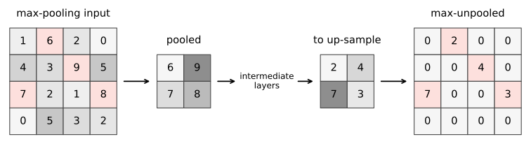
pp. 316–318 The efficient design down-samples as usual (strided convolutions, pooling) and then learns to up-sample back to the image resolution (Long, Shelhamer and Darrell, 2014; Noh, Hong and Han, 2015; Badrinarayanan, Kendall and Cipolla, 2015; Figure 10.27, a diagram). Fixed up-sampling layers reverse the poolings: copying each value into its \(2\times2\) block (an analogue of average pooling, Figure 10.28a), or placing it in the first cell of the block with zeros elsewhere (an analogue of max-pooling, Figure 10.28b). Placing it in the first cell is arbitrary; max-unpooling remembers, in each max-pooling layer, which cell held the maximum (the "switches") and puts the value back there in the matching up-sampling layer (Figure 10.29).
10.5.3 Fully convolutional networks
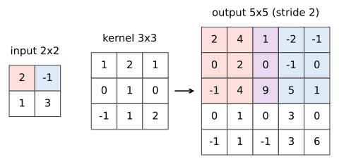
pp. 318–319 A learned up-sampling mirrors strided convolution. In a stride-2 convolution, one step on the output moves the filter two steps on the input; in the up-sampling, each input pixel is connected through the filter to a patch of the output, and one step on the input moves the patch two steps on the output (Dumoulin and Visin, 2016). Where patches overlap the contributions are summed (or averaged) (Figure 10.30). This is called a transposed convolution, because in matrix form it is the transpose of the matching convolution, or a fractionally strided convolution, the stride (output step per input step) being \(1/2\). "Deconvolution" is best avoided: in mathematics it means inverting a convolution, a different thing. A network with no pooling, down-sampling and up-sampling only by convolutions, is fully convolutional (Long, Shelhamer and Darrell, 2014): it takes an image of any size and returns a segmentation map of the same size.
Result 10.9 (up-sampling layers are adjoints of down-sampling layers) pp. 316–319; Exercise 10.13
- Transposed convolution. If \(\by=\bA\bx\) is a convolution with stride \(S\) (and padding \(P\)), the transposed convolution with the same filter and output stride \(S\) is \(\bz\mapsto\bA^\T\bz\): \(\langle\bA\bx,\bz\rangle\)\({}=\langle\bx,\bA^\T\bz\rangle\) for all \(\bx,\bz\). Each input value \(z_i\) adds \(z_i\,w_l\) to output position \(iS+l-P\); the output has \((n-1)S+M-2P\) positions for \(n\) inputs (before any cropping to a requested size). Equivalently: insert \(S-1\) zeros between the inputs, pad by \(M-1-P\) and apply an ordinary stride-1 convolution with the flipped filter.
- Pooling. Average pooling with \(k\times k\) windows and stride \(k\) has adjoint \(\frac1{k^2}\times\)(copy-unpooling); copy-unpooling is a right inverse of average pooling. At fixed switches, max-pooling is a selection matrix whose adjoint is max-unpooling; first-cell unpooling followed by max-pooling returns the input only if the input is non-negative.
- The backward pass of each down-sampling layer is its adjoint applied to the error signals (Result 10.4): so up-sampling layers are what backpropagation through the down-sampling layers already computes, used now in the forward direction with their own learned weights.
Uneven overlaps: when the filter size is not a multiple of the stride, output positions receive different numbers of stamps (in Figure 10.30 the middle row and column receive two stamps, their centre four, and every other position one), which can leave a periodic "checkerboard" pattern in the output.
Proof
(1) Row \(i\) of \(\bA\) holds the filter at columns \(iS-P,\dots,iS-P+M-1\) (indices in the unpadded input), so \((\bA^\T\bz)_c\)\({}=\sum_iA_{ic}z_i\)\({}=\sum_iz_iw_{c-iS+P}\): each \(z_i\) contributes \(z_iw_l\) at \(c=iS+l-P\), the stamping rule. The largest index reached is \((n-1)S+M-1-P\) and the smallest \(-P\); keeping indices \(0,\dots\) after cropping \(P\) on each side gives \((n-1)S+M-2P\) positions. Inserting zeros and convolving with the flipped filter is the same sum written from the output's point of view (Filling the gap 10.3). Exercise 10.13 is the case \(n=4\), \(M=3\), \(P=1\), \(S=2\) worked out below; numerical tests confirm \(\langle\bA\bx,\bz\rangle\)\({}=\langle\bx,\bA^\T\bz\rangle\) in two dimensions and that our transposed convolution equals PyTorch's.
(2) Average pooling: \(\langle\mathrm{avg}(X),Z\rangle\)\({}=\sum_{\bm u}Z_{\bm u}\frac1{k^2}\sum_{\bm n\in w(\bm u)}X_{\bm n}\)\({}=\sum_{\bm n}X_{\bm n}\frac1{k^2}Z_{\bm u(\bm n)}\), where \(\bm u(\bm n)\) is the window containing \(\bm n\); the right side is \(\langle X,\frac1{k^2}\mathrm{copy}(Z)\rangle\). Averaging a block of \(k^2\) copies of a value returns it. Max-pooling at fixed switches is \(X\mapsto(X_{\bm p(\bm u)})_{\bm u}\), a selection matrix with one 1 per row; its transpose puts \(Z_{\bm u}\) at \(\bm p(\bm u)\) and zeros elsewhere, which is max-unpooling. First-cell unpooling followed by max-pooling returns \(\max(z,0,0,0)\) for each value \(z\), which is \(z\) iff \(z\ge0\). Numerical tests confirm all of these against PyTorch's pooling and unpooling functions. (The book's statement that max-pooling regenerates the input of Figure 10.28(b) tacitly assumes non-negative values; in a network the pooled maps come after a ReLU, so this holds there.)
(3) The chain rule through a linear map \(\by=\bA\bx\) gives \(\partial E/\partial\bx\)\({}=\bA^\T\partial E/\partial\by\); for max-pooling, \(\bA\) is the selection matrix at the current switches. ∎
10.5.4 The U-net architecture
pp. 319–320 Down-sampling lets the number of channels grow without an explosion of units, but it throws away the positional detail that segmentation needs. The U-net (Ronneberger, Fischer and Brox, 2015; Figure 10.31, a diagram) pairs each down-sampling stage with an up-sampling stage and concatenates the last feature maps of each down-sampling stage with the first maps of the matching up-sampling stage (skip connections), giving the up-sampling path access to high-resolution information. A final \(1\times1\) convolution (Filling the gap 10.7) maps the channels to the \(C\) classes, followed by a per-pixel softmax.
10.6 Style Transfer
pp. 320–321 Early layers detect edges and textures, later layers objects (Section 10.3). Neural style transfer (Gatys, Ecker and Bethge, 2015) exploits this to render the content of an image \(C\) in the style of an image \(S\) (Figure 10.32): find a synthetic image \(G\) minimising
\[ E(G)=E_{\rm content}(G,C)+E_{\rm style}(G,S) \tag{10.13} \]by gradient descent on the pixels of \(G\), starting from a random image, with the weights of a trained network fixed. Content is compared position by position at one chosen layer,
\[ E_{\rm content}(G,C)=\sum_{i,j,k}\{a_{ijk}(G)-a_{ijk}(C)\}^2, \tag{10.14} \]with \(a_{ijk}(G)\) the pre-activation at position \((i,j)\) of channel \(k\) for input \(G\); an early layer preserves edges, a later one only objects. Style is taken to be which features occur together, wherever they are: for each pair of channels, the style matrix
\[ F_{kk'}(G)=\sum_{i=1}^{I}\sum_{j=1}^{J}a_{ijk}(G)\,a_{ijk'}(G), \tag{10.15} \]for an \(I\times J\) map with \(K\) channels, and
\[ E_{\rm style}(G,S)=\frac1{(2IJK)^2}\sum_{k=1}^{K}\sum_{k'=1}^{K}\{F_{kk'}(G)-F_{kk'}(S)\}^2. \tag{10.16} \]Better results come from several layers,
\[ E_{\rm style}(G,S)=\sum_l\lambda_lE^{(l)}_{\rm style}(G,S), \tag{10.17} \]with weights \(\lambda_l\) set by eye; they also set the balance with the content term.
Erratum. p. 321 "In defining \(E_{\rm style}(G,C)\)" should read \(E_{\rm style}(G,S)\): the style error compares \(G\) with the style image.
Result 10.10 (the style matrix and the gradients of the two errors) pp. 320–321, (10.14)–(10.16)
Write the layer's pre-activations for \(G\) as a matrix \(\bA\in\R^{K\times IJ}\) (row \(k\) is channel \(k\), flattened). Then:
- \(\bF=\bA\bA^\T\): symmetric and positive semi-definite, equal to \(IJ\) times the (uncentred) second-moment matrix of the \(K\)-dimensional feature vectors over positions, and unchanged by any permutation of the positions. It records which features co-occur, not where.
- The gradients of the two errors with respect to the pre-activations are \[\frac{\partial E_{\rm content}}{\partial\bA}=2\big(\bA(G)-\bA(C)\big),\qquad \frac{\partial E_{\rm style}}{\partial\bA}=\frac{1}{(IJK)^2}\big(\bF(G)-\bF(S)\big)\bA(G).\]
- The factor \(1/(2IJK)^2\) in (10.16) is the \(1/(4N^2M^2)\) of Gatys et al. with \(N=K\) channels and \(M=IJ\) positions; it makes layers of different sizes comparable before the weights \(\lambda_l\).
The pixel gradient follows by backpropagating these matrices through the fixed network (Result 10.4).
Proof
(1) \(F_{kk'}\)\({}=\sum_{\bm n}A_{k\bm n}A_{k'\bm n}\)\({}=(\bA\bA^\T)_{kk'}\); for any \(\bv\), \(\bv^\T\bA\bA^\T\bv=\|\bA^\T\bv\|^2\ge0\). Dividing by the number \(IJ\) of positions gives the average of \(\ba_{\bm n}\ba_{\bm n}^\T\) over positions \(\bm n\), where \(\ba_{\bm n}\in\R^K\) is the feature vector at \(\bm n\). A permutation \(\bPi\) of positions maps \(\bA\) to \(\bA\bPi\) and \(\bA\bPi\bPi^\T\bA^\T=\bA\bA^\T\). (So matching Gram matrices matches second moments of the feature distribution, a quadratic-kernel version of matching distributions; Li et al., 2017.)
(2) The content gradient is immediate. For the style, with \(\bm\Delta=\bF(G)-\bF(S)\) (symmetric) and \(c=1/(2IJK)^2\), \(E_{\rm style}=c\Tr(\bm\Delta^2)\) and \(\d E_{\rm style}=2c\Tr(\bm\Delta\,\d\bF)\), \(\d\bF=\d\bA\,\bA^\T+\bA\,\d\bA^\T\). So \(\d E_{\rm style}\)\({}=2c\{\Tr(\bm\Delta\,\d\bA\,\bA^\T)\)\({}+\Tr(\bm\Delta\bA\,\d\bA^\T)\}\)\({}=4c\Tr(\bA^\T\bm\Delta\,\d\bA)\) using the cyclic property and the symmetry of \(\bm\Delta\), hence \(\partial E_{\rm style}/\partial\bA\)\({}=4c\,\bm\Delta\bA\)\({}=\bm\Delta\bA/(IJK)^2\) (see the matrix calculus section of the companion course's toolkit). A numerical test compares this with automatic differentiation.
(3) \((2IJK)^2=4K^2(IJ)^2\). ∎
Algorithm 10.4 (neural style transfer) pp. 320–321
- Fix a trained network. Record \(a(C)\) at the content layer and \(\bF^{(l)}(S)\) at the style layers.
- Initialise \(G\) randomly. Repeat: forward-propagate \(G\); evaluate (10.13) with (10.14), (10.16), (10.17); backpropagate to the pixels (Result 10.10); take a gradient step (we use Adam) and clip the pixels to their valid range.
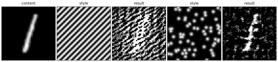
Summary: errors and imprecisions found in the chapter (first printing) and in the solutions manual
- (10.5), p. 294: the output size is \(\floor{(J+2P-M)/S}+1\), not \(\floor{(J+2P-M)/S-1}\) (Result 10.2; for the \(3\times3\) image of Figure 10.3 the printed formula gives 0 instead of 2). The manual's Solution 10.7 is correct.
- (10.20), p. 322: the "flipped form" of the convolution in Exercise 10.4 is printed identical to the cross-correlation (10.2); the kernel must be flipped, \(\widetilde K(l,m)=K(L-1-l,M-1-m)\), and the image index shifted (as the manual's (392)–(394) do).
- p. 301: "most of the connections are in the first convolutional layer" of VGG-16: the first layer holds 0.6% of the connections; the convolutional layers together hold 99.2% (Figure 10.10).
- p. 312: the pooling of Figure 10.22 has stride 2, not 1.
- p. 317: max-pooling regenerates the input of Figure 10.28(b) only for non-negative values (Result 10.9).
- p. 321: \(E_{\rm style}(G,C)\) should be \(E_{\rm style}(G,S)\).
- p. 305 (a difference, not an error): the book's Grad-CAM (10.10) weights pre-activations and has no final ReLU; Selvaraju et al. use the activations after the ReLU and apply a ReLU to the map. On our network the pre-activation form lights up background where negative weights meet negative pre-activations (Figure 10.15).
- Solutions manual, Solution 10.8: the parameter counts and the total of 138,357,544 are right, but eight of the connection counts are not: conv 1 has \(224^2\cdot28\cdot64=89{,}915{,}392\) connections (not 96,337,920) and conv layers 4–10 are given the values of layers of the same spatial size but different input channels (e.g. conv 4: \(112^2\cdot1153\cdot128=1{,}851{,}293{,}696\), not 1,852,899,328); the correct total is 15,483,821,032, not 15,504,292,840.
- Solutions manual, Solution 10.12: it states that an inner product of length \(N\) costs \(2N-1\) steps but then charges \(9\times8=72\) steps (instead of 17) per \(3\times3\) filter, and compares 8 rather than the requested 9 naive passes; with consistent counting the passes cost 291 and 667 steps and the ratio for nine passes is 3.93 (the manual's 3.54). Also, the large network evaluates only 4 of the 9 window positions (Result 10.8), so the like-for-like ratio is 1.75.
Exercises
All 13 exercises of Chapter 10 (Bishop and Bishop, 2024, pp. 322–324), restated in my own words, with complete solutions (hidden). Stars give the book's difficulty. Each was solved independently and then compared with the official solutions manual; where they differ, the solution says so and why.
Exercise 10.1 (★). For a fixed \(\bw\), show with a Lagrange multiplier that the \(\bx\) maximising \(\bw^\T\bx\) subject to a fixed \(\|\bx\|^2\) is a multiple of \(\bw\).
Solution
Stationary points of \(\mathcal L=\bw^\T\bx+\lambda(\|\bx\|^2-r^2)\): \(\nabla_\bx\mathcal L=\bw+2\lambda\bx=\bzero\), so \(\bx=-\bw/(2\lambda)=\alpha\bw\). The constraint gives \(|\alpha|=r/\|\bw\|\); \(\alpha>0\) is the maximum (value \(r\|\bw\|\)) and \(\alpha<0\) the minimum. Cauchy–Schwarz confirms this is the global maximum (Filling the gap 10.2; method in the companion toolkit). Same as the manual, which does not separate the two signs.
Exercise 10.2 (★★). A one-dimensional convolutional layer has 5 inputs and a width-3 filter with stride 1. Write it as a fully connected layer whose missing connections are zeros and whose shared weights are repeated entries (no biases).
Solution
With filter \((k_1,k_2,k_3)\), \(\by=\bA\bx\) with \(\bA\)\({}=\begin{pmatrix}k_1&k_2&k_3&0&0\\0&k_1&k_2&k_3&0\\0&0&k_1&k_2&k_3\end{pmatrix}\): a \(3\times5\) Toeplitz matrix, 9 connections, 3 parameters (Filling the gap 10.4; checked). Same as the manual.
Exercise 10.3 (★). Compute the convolution (10.2) of the \(4\times4\) array with rows \((2,5,-3,0)\), \((0,6,0,-4)\), \((-1,-3,0,2)\), \((5,0,0,3)\) with the \(2\times2\) filter with rows \((-2,0)\), \((4,6)\) (10.18).
Solution
Each entry is \(-2\times\)(top-left) \(+\,4\times\)(bottom-left) \(+\,6\times\)(bottom-right) of the \(2\times2\) window; e.g. the first is \(-2\cdot2+0\cdot5+4\cdot0+6\cdot6=32\). The \(3\times3\) result has rows \((32,14,-18)\), \((-22,-24,12)\), \((22,6,18)\) (checked). Same as the manual.
Exercise 10.4 (★★). For a \(J\times K\) image and an \(L\times M\) filter, give the summation limits in (10.2); do the same for the mathematical convolution \(C(j,k)=\sum_{l,m}I(j-l,k-m)K(l,m)\) (10.19), and show that it can be written in a "flipped" cross-correlation form (10.20), with its limits.
Solution
Index the image by \(1\le j\le J\), \(1\le k\le K\) and the filter by \(1\le l\le L\), \(1\le m\le M\) (the book's convention). (10.2): \(C(j,k)\)\({}=\sum_{l=1}^L\sum_{m=1}^MI(j+l,k+m)K(l,m)\), defined when \(1\le j+l\le J\) for all \(l\), i.e. \(0\le j\le J-L\), and \(0\le k\le K-M\). (10.19): the same sums; \(1\le j-l\le J\) for all \(l\) requires \(L+1\le j\le J+1\), and \(M+1\le k\le K+1\). Flipped form: put \(\lambda=L+1-l\), \(\mu=M+1-m\) (so \(\lambda,\mu\) run over the same ranges): \[C(j,k)=\sum_{\lambda=1}^{L}\sum_{\mu=1}^{M}I(j'+\lambda,\,k'+\mu)\,\widetilde K(\lambda,\mu),\qquad j'=j-L-1,\ k'=k-M-1,\ \widetilde K(\lambda,\mu)=K(L+1-\lambda,M+1-\mu),\] with \(0\le j'\le J-L\), \(0\le k'\le K-M\): a cross-correlation with the flipped filter. Same as the manual's (390)–(394). Erratum: (10.20) as printed, \(\sum_{l,m}I(j+l,k+m)K(l,m)\), is just (10.2) again; the flip of \(K\) is missing (Filling the gap 10.3).
Exercise 10.5 (★). Relate the continuous convolution \(F(x)=\int G(y)k(x-y)\,\d y\) (10.21) to the convolutional layer (10.19) through a discrete approximation.
Solution
Substitute \(z=x-y\): \(F(x)=\int G(x-z)k(z)\,\d z\). On a grid of spacing \(\Delta\), \(F(j\Delta)\)\({}\approx\sum_lG((j-l)\Delta)\,k(l\Delta)\,\Delta\), which is the one-dimensional (10.19) with \(C(j)=F(j\Delta)\), \(I(n)=G(n\Delta)\) and kernel \(K(l)=k(l\Delta)\Delta\); a kernel of finite width corresponds to \(k\) vanishing outside a bounded interval. A CNN learns the samples \(K(l)\) of the kernel directly. Checked on two Gaussians (error below \(10^{-6}\)). Same as the manual.
Exercise 10.6 (★). An image \(J\times K\) padded by \(P\) pixels on all sides is convolved with an \(M\times M\) kernel, \(M\) odd. Show that \(P=(M-1)/2\) gives a \(J\times K\) feature map.
Solution
The map is \((J+2P-M+1)\times(K+2P-M+1)\) (Result 10.2 with \(S=1\)); \(2P=M-1\) gives \(J\times K\). \(P\) is an integer because \(M\) is odd. Same as the manual.
Exercise 10.7 (★). Show that an \(M\times M\) kernel on a \(J\times K\) image with padding \(P\) and stride \(S\) gives a feature map of the size (10.5).
Solution
The admissible first rows of the filter are \(iS\) with \(0\le iS\le J+2P-M\), so there are \(\floor{(J+2P-M)/S}+1\) of them, and likewise for columns (Result 10.2, which also covers dilation). This agrees with the manual's answer, \(\floor{(J+2P-M)/S+1}\), and shows that the printed (10.5), with \(-1\), is wrong.
Exercise 10.8 (★★). For each of the 16 learnable layers of VGG-16 (Figure 10.10), find (i) the number of connections, biases included, and (ii) the number of learnable parameters; check that the parameters total about 138 million.
Solution
A \(3\times3\) same convolution from \(C_{\rm in}\) to \(C_{\rm out}\) channels on an \(H\times H\) map: each of the \(H^2C_{\rm out}\) units has \(9C_{\rm in}+1\) incoming connections (counting padding inputs, as the manual does), so \(H^2(9C_{\rm in}+1)C_{\rm out}\) connections and \((9C_{\rm in}+1)C_{\rm out}\) parameters. A fully connected layer has \((n_{\rm in}+1)n_{\rm out}\) of each.
layer map \(C_{\rm in}\to C_{\rm out}\) connections parameters conv 1 224 3 → 64 89,915,392 1,792 conv 2 224 64 → 64 1,852,899,328 36,928 conv 3 112 64 → 128 926,449,664 73,856 conv 4 112 128 → 128 1,851,293,696 147,584 conv 5 56 128 → 256 925,646,848 295,168 conv 6 56 256 → 256 1,850,490,880 590,080 conv 7 56 256 → 256 1,850,490,880 590,080 conv 8 28 256 → 512 925,245,440 1,180,160 conv 9 28 512 → 512 1,850,089,472 2,359,808 conv 10 28 512 → 512 1,850,089,472 2,359,808 conv 11–13 (each) 14 512 → 512 462,522,368 2,359,808 fc 1 25,088 → 4,096 102,764,544 102,764,544 fc 2 4,096 → 4,096 16,781,312 16,781,312 fc 3 4,096 → 1,000 4,097,000 4,097,000 total 15,483,821,032 138,357,544 So about 138.4 million parameters, 74% of them in fc 1, while 99.2% of the connections are in the convolutional layers (Figure 10.10). Comparison. The manual's parameters agree. Its connection counts for conv 1 (96,337,920) and conv 4–10 are wrong: conv 1 is \(224^2\cdot28\cdot64=89{,}915{,}392\), and conv 4–10 repeat the values of the earlier layer of the same spatial size, ignoring that \(C_{\rm in}\) doubled (e.g. conv 4 has \(112^2\cdot1153\cdot128\), not \(112^2\cdot577\cdot256\)); its total 15,504,292,840 should be 15,483,821,032 (checked).
Exercise 10.9 (★★). If the kernel of (10.2) is separable, \(K(l,m)=F(l)G(m)\) (10.22), show that the two-dimensional convolution can be done as two one-dimensional ones, and that this is much cheaper.
Solution
\(C(j,k)\)\({}=\sum_lF(l)\big[\sum_mI(j+l,k+m)G(m)\big]\)\({}=\sum_lF(l)\,R(j+l,k)\), where \(R=I\star G\) row by row (\(J\times(K-M+1)\) values, \(M\) multiply-adds each) and then \(C=R\star F\) column by column (\((J-L+1)(K-M+1)\) values, \(L\) each). Cost \(J(K-M+1)M\)\({}+(J-L+1)(K-M+1)L\)\({}\approx JK(L+M)\) against \((J-L+1)(K-M+1)LM\approx JKLM\) directly: for a \(7\times7\) kernel, 14 instead of 49 per pixel. Storage drops from \(LM\) to \(L+M\). The price: separable kernels have rank one, a strong restriction (a learned kernel can be approximated by a sum of a few separable ones, using its singular value decomposition). Checked on a \(20\times17\) image. Same as the manual (which uses the convolution form (10.19); the count is identical).
Exercise 10.10 (★). Show that DeepDream (setting the backpropagation \(\delta\)'s of the chosen layer to its pre-activations and backpropagating to the pixels) is gradient-based optimisation of (10.12).
Solution
\(\partial F/\partial a_{ijk}=2a_{ijk}\), and backpropagation is linear in the starting \(\delta\)'s, so starting from \(\delta=a\) yields \(\frac12\nabla_IF\) (Filling the gap 10.11; checked against autograd). Same as the manual.
Exercise 10.11 (★★). A detector for \(C\) classes can output a softmax over \(C+1\) classes (the last one "background"), or a probability that an object is present together with a distribution over the \(C\) classes. Relate the two.
Solution
Let \(p_f(i)\), \(i=1,\dots,C+1\), be the first model's outputs, \(p_g\) the presence probability and \(p_h(i)\) the class distribution given an object. By the product rule (companion course, Section 1.2), \[p_f(i)=p_g\,p_h(i)\quad(i\le C),\qquad p_f(C+1)=1-p_g.\] Conversely \(p_g=1-p_f(C+1)\) and \(p_h(i)=p_f(i)/(1-p_f(C+1))\) when \(p_f(C+1)<1\). Both parametrisations have \(C\) free probabilities, so they describe the same set of distributions (the factorised one leaves \(p_h\) undefined when \(p_g=0\)). The difference is in training: the factorised form lets the box regression and class loss be switched off for background windows, and the presence and class outputs can be trained with separate losses. Same as the manual, plus the converse (checked on a numerical example).
Exercise 10.12 (★★). Count the operations of one forward pass through the network of Figure 10.22 (ignoring biases and activation functions), and through the enlarged network of Figure 10.23 on an \(8\times8\) image; then find the ratio of the cost of nine naive applications of the small network to one pass of the large one.
Solution
Count an inner product of length \(N\) as \(N\) multiplications and \(N-1\) additions, \(2N-1\) steps, and a maximum of 4 numbers as 3 comparisons. \(6\times6\) network: the \(3\times3\) convolution has \(4\times4=16\) outputs at 17 steps each, 272; the \(2\times2\) pooling (stride 2; see the erratum) has 4 outputs at 3 steps, 12; the output is an inner product of length 4, 7 steps. Total 291. \(8\times8\) network: \(6\times6=36\) convolution outputs, 612; \(3\times3=9\) pooled outputs, 27; \(2\times2=4\) outputs at 7 steps, 28. Total 667. Ratios: nine passes of the small network over the nine \(6\times6\) windows of an \(8\times8\) image cost \(9\times291=2{,}619\) steps, \(2{,}619/667=3.93\) times one pass of the large network. But the large network evaluates only the 4 windows at even offsets (Result 10.8); the like-for-like ratio is \(4\times291/667=1.75\). Comparison. The manual uses the rule \(2N-1\) but then charges \(9\times8=72\) steps per \(3\times3\) filter (instead of 17), getting 1,171 and 2,647, and divides 8 (not 9) passes by one, 3.54. The two slips partly cancel (with its counts, nine passes would give 3.98); with consistent counting the answer is 3.93 (checked).
Exercise 10.13 (★★). A one-dimensional input \((x_1,x_2,x_3,x_4)\) is zero-padded to \((0,x_1,x_2,x_3,x_4,0)\) and convolved with the filter \((w_1,w_2,w_3)\) with stride 2. Write the output as \(\bA\) times the padded vector. Then up-sample \((z_1,z_2)\) with the same filter and output stride 2, summing overlaps, to a six-dimensional vector, and show that this is multiplication by \(\bA^\T\).
Solution
With stride 2 the filter fits at positions 0 and 2 of the 6-vector (position 4 would need a seventh entry), so \(y_1=w_2x_1+w_3x_2\), \(y_2=w_1x_2+w_2x_3+w_3x_4\), and \[\bA=\begin{pmatrix}w_1&w_2&w_3&0&0&0\\0&0&w_1&w_2&w_3&0\end{pmatrix}.\] The up-sampling places \(z_1(w_1,w_2,w_3)\) at positions 1–3 and \(z_2(w_1,w_2,w_3)\) at positions 3–5 of a 6-vector: \[\bh=(w_1z_1,\ w_2z_1,\ w_3z_1+w_1z_2,\ w_2z_2,\ w_3z_2,\ 0).\] Column \(i\) of \(\bA^\T\) is row \(i\) of \(\bA\), so \[\bA^\T\bz=z_1(w_1,w_2,w_3,0,0,0)+z_2(0,0,w_1,w_2,w_3,0)=\bh.\] This is Result 10.9(1) (checked). Same as the manual.
Demonstrations
Three interactive pages, each linked above where its topic arises. The two network demos load the weights of our trained network (data/ch10-cnn.json, rounded to 7 significant digits) and run it in JavaScript, including backpropagation to the pixels. All three reproduce the Python numbers (maximum differences: 0 for the convolution calculator, \(9\times10^{-15}\) for the logits, \(8\times10^{-16}\) for Grad-CAM, \(1.2\times10^{-14}\) for the adversarial attacks).
- Convolution arithmetic: the book's convolution (a cross-correlation), the flipped mathematical convolution and the transposed convolution on a small image, with any filter, padding, stride and dilation; click a cell to see its receptive field or its stamp. Presets: 1 vertical edges (Figures 10.3, 10.4), 2 same padding, 3 stride 2 and (10.5), 4 dilation, 5 convolution versus cross-correlation, 6 transposed convolution (Figure 10.30).
- Inside a small convolutional network: learned filters, the feature maps of all three layers, equivariance under shifts and Grad-CAM in both forms, on test digits or on your own drawing. Presets: 1 filters and maps, 2 equivariance, 3 deeper layers, 4 Grad-CAM, 5 background.
- Adversarial examples: the fast gradient sign method (10.11), random signs of the same size, the iterative and the targeted versions, with the probability of the true class against \(\epsilon\) and the first-order bound \(\epsilon\|\bg\|_1\). Presets: 1 small \(\epsilon\), 2 Figure 10.16, 3 random signs, 4 iterative, 5 targeted.
References
- Bishop, C. M. and Bishop, H. (2024). Deep Learning: Foundations and Concepts. Springer, Cham. Chapter 10, pp. 287–324. doi:10.1007/978-3-031-45468-4. Book website: www.bishopbook.com.
- Bishop, C. M. and Bishop, H. (2024). Deep Learning: Foundations and Concepts, Solutions to Exercises, version 1.0 (Chapters 2–10).
- Badrinarayanan, V., Kendall, A. and Cipolla, R. (2015). SegNet: a deep convolutional encoder-decoder architecture for image segmentation. arXiv preprint.
- Deng, J., Dong, W., Socher, R., Li, L.-J., Li, K. and Fei-Fei, L. (2009). ImageNet: a large-scale hierarchical image database. In IEEE Conference on Computer Vision and Pattern Recognition, 248–255.
- Dumoulin, V. and Visin, F. (2016). A guide to convolution arithmetic for deep learning. arXiv:1603.07285.
- Eykholt, K. et al. (2018). Robust physical-world attacks on deep learning visual classification. In IEEE Conference on Computer Vision and Pattern Recognition.
- Fukushima, K. (1980). Neocognitron: a self-organizing neural network model for a mechanism of pattern recognition unaffected by shift in position. Biological Cybernetics, 36, 193–202.
- Gatys, L. A., Ecker, A. S. and Bethge, M. (2015). A neural algorithm of artistic style. arXiv:1508.06576.
- Girshick, R. (2015). Fast R-CNN. In IEEE International Conference on Computer Vision.
- Goodfellow, I. J., Shlens, J. and Szegedy, C. (2014). Explaining and harnessing adversarial examples. arXiv:1412.6572.
- Hubel, D. H. and Wiesel, T. N. (1959). Receptive fields of single neurones in the cat's striate cortex. The Journal of Physiology, 148, 574–591.
- Hyvärinen, A., Hurri, J. and Hoyer, P. O. (2009). Natural Image Statistics: A Probabilistic Approach to Early Computational Vision. Springer.
- Krizhevsky, A., Sutskever, I. and Hinton, G. E. (2012). ImageNet classification with deep convolutional neural networks. In Advances in Neural Information Processing Systems 25.
- LeCun, Y. et al. (1989). Backpropagation applied to handwritten zip code recognition. Neural Computation, 1(4), 541–551.
- LeCun, Y., Bottou, L., Bengio, Y. and Haffner, P. (1998). Gradient-based learning applied to document recognition. Proceedings of the IEEE, 86(11), 2278–2324.
- Li, Y., Wang, N., Liu, J. and Hou, X. (2017). Demystifying neural style transfer. In Proceedings of the 26th International Joint Conference on Artificial Intelligence.
- Lin, M., Chen, Q. and Yan, S. (2013). Network in network. arXiv:1312.4400.
- Long, J., Shelhamer, E. and Darrell, T. (2014). Fully convolutional networks for semantic segmentation. arXiv:1411.4038.
- Luo, W., Li, Y., Urtasun, R. and Zemel, R. (2016). Understanding the effective receptive field in deep convolutional neural networks. In Advances in Neural Information Processing Systems 29.
- Mordvintsev, A., Olah, C. and Tyka, M. (2015). Inceptionism: going deeper into neural networks. Research blog post.
- Noh, H., Hong, S. and Han, B. (2015). Learning deconvolution network for semantic segmentation. In IEEE International Conference on Computer Vision.
- Redmon, J., Divvala, S., Girshick, R. and Farhadi, A. (2015). You only look once: unified, real-time object detection. arXiv:1506.02640.
- Ren, S., He, K., Girshick, R. and Sun, J. (2015). Faster R-CNN: towards real-time object detection with region proposal networks. In Advances in Neural Information Processing Systems 28.
- Ronneberger, O., Fischer, P. and Brox, T. (2015). U-Net: convolutional networks for biomedical image segmentation. In Medical Image Computing and Computer-Assisted Intervention (MICCAI).
- Selvaraju, R. R., Cogswell, M., Das, A., Vedantam, R., Parikh, D. and Batra, D. (2016). Grad-CAM: visual explanations from deep networks via gradient-based localization. arXiv:1610.02391.
- Sermanet, P., Eigen, D., Zhang, X., Mathieu, M., Fergus, R. and LeCun, Y. (2013). OverFeat: integrated recognition, localization and detection using convolutional networks. arXiv:1312.6229.
- Simonyan, K., Vedaldi, A. and Zisserman, A. (2013). Deep inside convolutional networks: visualising image classification models and saliency maps. arXiv preprint.
- Simonyan, K. and Zisserman, A. (2014). Very deep convolutional networks for large-scale image recognition. arXiv:1409.1556.
- Szegedy, C., Zaremba, W., Sutskever, I., Bruna, J., Erhan, D., Goodfellow, I. and Fergus, R. (2013). Intriguing properties of neural networks. arXiv:1312.6199.
- Yosinski, J., Clune, J., Nguyen, A., Fuchs, T. and Lipson, H. (2015). Understanding neural networks through deep visualization. arXiv preprint.
- Yu, F. and Koltun, V. (2016). Multi-scale context aggregation by dilated convolutions. In International Conference on Learning Representations.
- Zeiler, M. D. and Fergus, R. (2013). Visualizing and understanding convolutional networks. arXiv:1311.2901.
- Zhou, B., Khosla, A., Lapedriza, A., Oliva, A. and Torralba, A. (2016). Learning deep features for discriminative localization. In IEEE Conference on Computer Vision and Pattern Recognition.
Every numerical statement in these notes comes from ch10_convolutional_networks.py. The network was trained on the 60,000 MNIST training digits and evaluated on the 10,000 test digits.