Deep Neural Networks
A linear model in fixed basis functions can, in principle, approximate anything, but the number of basis functions it needs explodes with the input dimension. This chapter first makes that failure precise (the curse of dimensionality and the strange geometry of high-dimensional spaces, Section 6.1), then lets the basis functions themselves be learned: a multilayer network (Section 6.2) is a universal approximator, and stacking many layers (Section 6.3) buys exponentially more expressive power per parameter as well as a hierarchical, reusable representation of the data. The chapter ends with the error functions that turn a network into a probabilistic model (Section 6.4) and with mixture density networks, which predict a whole multimodal conditional distribution (Section 6.5). These notes prove every result the chapter states without proof, correct a few formulas, and reproduce its figures.
Ch. 1 Deep learning revolution Ch. 2 Probabilities Ch. 3 Standard distributions Ch. 4 Regression Ch. 5 Classification Ch. 6 Deep neural networks Ch. 7 Gradient descent Ch. 8 Backpropagation Ch. 9 Regularization Ch. 10 Convolutional networks Ch. 11 Structured distributions Ch. 12 Transformers Ch. 13 Graph neural networks Ch. 14 Sampling Ch. 15 Discrete latent variables Ch. 16 Continuous latent variables Ch. 17 GANs Ch. 18 Normalizing flows Ch. 19 Autoencoders Ch. 20 Diffusion models Appendices A to C
How to read these notes
They follow the book. Sections carry the book's numbers (6.2.2, 6.5.3, ...) and every displayed equation that appears in the book carries its number, e.g. (6.12). Equations without a number are steps that the book skips.
Filling the gaps. Wherever the chapter says that something "can be shown", leaves it to an exercise, or states a property without proof (universal approximation, the symmetry factor \(M!\,2^M\), the exponential number of linear regions, the gradients of the mixture density network), an orange Filling the gap box or a proof gives the full argument. Proofs start hidden: open one with its bar, or use the button below.
Figures and demonstrations. Every figure computed from data or a model is reproduced from scratch by the Python code; the schematic ones are redrawn or described. The ▶ Demo boxes open an interactive demonstration already set to the case being discussed.
Main reference
C. M. Bishop and H. Bishop, Deep Learning: Foundations and Concepts, Springer (2024), Chapter 6, pages 171–207 (book website www.bishopbook.com). Section, equation, figure and exercise numbers below refer to this book. Further reading is listed in the references.
The explanations, derivations, code and figures are my own; equations are cited by their numbers in the book.
Companion course: Bayesian and Probabilistic Machine Learning
Much of this chapter revisits Chapter 5 of Bishop (2006), which the companion course Bayesian and Probabilistic Machine Learning follows. Where a derivation is the same it is sketched here and proved in full there:
- The curse of dimensionality, volumes of spheres and the Gaussian shell: Chapter 1, Section 1.4 (Result 1.13, Result 1.14); fixed basis functions: Section 3.6; radial basis functions and support vector machines: Section 6.3 and Section 7.1.
- Feed-forward network functions, universal approximation, tanh and sigmoid units, weight-space symmetries: Section 5.1 (Result 5.1, Result 5.2, Filling the gap 5.2), and the backpropagation demo.
- Error functions as negative log likelihoods and the canonical link: Section 5.2 (Result 5.3, Result 5.4), and Section 4.3.6.
- Mixture density networks: Section 5.6 (Result 5.18, Result 5.19) and the mixture density demo; mixtures of experts: Section 14.5.3; autoencoders and nonlinear manifolds: Section 12.4.2.
What is new on this page: the grid classifier's data requirement, concentration of norms and distances, a complete proof of universal approximation in any dimension with approximation rates, saturation bounds and dead units, the exact rate at which swish tends to ReLU, the symmetry group and why ReLU networks have a continuum of equivalent weights, linear regions of ReLU networks with the arrangement bound and the sawtooth depth separation, the InfoNCE bounds and gradient, MDN gradients and moments for vector targets (with a correction to (6.50)), the robot-arm inverse kinematics, and a conditional-mode algorithm.
The chapter at a glance
- 6.1 A general polynomial of order \(M\) in \(D\) variables has \(\binom{D+M}{M}\) coefficients (Filling the gap 6.1); a grid classifier needs a number of points exponential in \(D\) (6.2). In high dimensions a ball's volume sits at its surface, a cube's in its corners, and a Gaussian's mass in a thin shell far from its mode (Result 6.1); norms and distances concentrate (6.3). Real data lie near low-dimensional manifolds, which is why learning is possible at all.
- 6.2 A two-layer network (Definition 6.1) learns its own basis functions. With any continuous non-polynomial activation it approximates every continuous function on a compact set (Result 6.2, proved in full). Activation functions and their derivatives, saturation and dead units (Result 6.3); every weight vector of a tanh network has \(M!\,2^M\) equivalent partners, while ReLU networks have a continuum (Result 6.4).
- 6.3 A ReLU network is piecewise linear. One layer of \(M\) units on \(\R^D\) has at most \(\sum_{j\le D}\binom Mj\) linear regions (Result 6.5); \(L\) layers of 2 units can have \(2^L\), which a one-layer network needs \(2^L-1\) units to match (Result 6.6). Hierarchical, distributed and transferable representations; the InfoNCE loss is a cross-entropy with bounded logits (6.8).
- 6.4 Each error function is a negative log likelihood, and with the matching output activation the error signal is \(y_k-t_k\) (Result 6.7).
- 6.5 A mixture density network (Definition 6.3) outputs the parameters of a Gaussian mixture; its gradients are (6.45)–(6.47) (Result 6.8) and its predictive mean and variance are (6.48) and the corrected (6.50) (Result 6.9).
Notation. Inputs \(\x\in\R^D\), targets \(\tv\in\R^K\) (or \(\R^L\) in Section 6.5), data \(\{(\x_n,\tv_n)\}_{n=1}^N\). A network has \(M\) hidden units in a layer; \(a\) is a pre-activation, \(z=h(a)\) a hidden-unit output, \(\sigma(a)=1/(1+e^{-a})\) the logistic sigmoid and \(\relu(a)=\max(0,a)\). All weights and biases form one vector \(\w\); \(E(\w)=\sum_nE_n(\w)\). Biases are absorbed as weights from a unit fixed at 1 (\(x_0=z_0=1\)).
Printing and corrections. The text used is the first edition (2024). Where an equation does not follow from its own derivation the notes say so in an Erratum note with the evidence: the Gaussian-shell expansion (6.59) (Result 6.1), the variance (6.50) for vector targets (Result 6.9), and a few smaller slips. Corrections to the official solutions manual are noted at the exercises.
6.1 Limitations of Fixed Basis Functions
pp. 172–179 The models of Chapters 4 and 5 are linear combinations of fixed basis functions passed through an output nonlinearity,
\[ y(\x,\w)=f\Big(\sum_{j=1}^{M}w_j\phi_j(\x)+w_0\Big), \tag{6.1} \]with \(f\) the identity for regression. Because the \(\phi_j\) are arbitrary, such a model can represent any input–output map if one of the \(\phi_j\) happens to be that map, and a rich enough family should approximate any map. The catch is that the \(\phi_j\) are chosen before seeing the data, and the number needed grows explosively with the input dimension \(D\).
See also: Section 3.6, limitations of fixed basis functions, in the companion course.
6.1.1 The curse of dimensionality
pp. 172–175 A polynomial of order \(M\) in one variable,
\[ y(x,\w)=w_0+w_1x+w_2x^2+\dots+w_Mx^M, \tag{6.2} \]has \(M+1\) coefficients. With \(D\) inputs, a general polynomial up to order 3 is
\[ y(\x,\w)=w_0+\sum_{i=1}^{D}w_ix_i+\sum_{i=1}^{D}\sum_{j=1}^{D}w_{ij}x_ix_j+\sum_{i=1}^{D}\sum_{j=1}^{D}\sum_{k=1}^{D}w_{ijk}x_ix_jx_k , \tag{6.3} \]and the book states that the number of independent coefficients grows like \(D^3\), and like \(D^M\) for order \(M\).
Filling the gap 6.1: counting the coefficients of a polynomial in \(D\) variables p. 173
(6.3) is written with \(D^2\) coefficients \(w_{ij}\) and \(D^3\) coefficients \(w_{ijk}\), but \(x_ix_j=x_jx_i\), so only symmetric combinations matter. How many are independent?
Derivation
Count. A monomial of degree at most \(M\) is \(x_1^{k_1}\cdots x_D^{k_D}\) with \(k_i\ge0\) and \(k_1+\dots+k_D\le M\). Add a slack variable \(k_0=M-\sum_ik_i\ge0\); the monomials are then in one-to-one correspondence with the solutions of \(k_0+k_1+\dots+k_D=M\) in non-negative integers. By "stars and bars" (place \(M\) stars and \(D\) bars in a row; the counts between bars are \(k_0,\dots,k_D\)) there are
\[ \binom{D+M}{M}=\frac{(D+M)!}{D!\,M!} \]of them. For \(M=3\), \(D=4\) this is 35, which enumeration confirms. Distinct monomials are linearly independent functions, so this is exactly the number of free coefficients.
Growth. For fixed \(M\), \(\binom{D+M}{M}\)
The Iris data (Fisher 1936) make the point for classification. With only the two sepal measurements we would like to classify the test point × in Figure 6.1 from its neighbours. The simplest way to use "neighbourhood" is a grid: cut each axis into \(k\) intervals, and label a test point with the majority class of the training points in its cell.
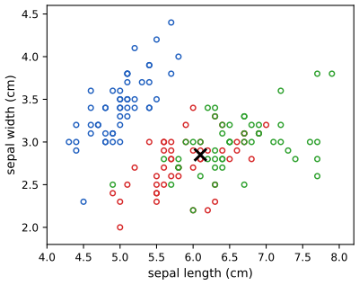
fig_6_1. Download: PDF · SVGAlgorithm 6.1 (grid classifier) pp. 173–174
- Choose a box containing the data and cut each of its \(D\) axes into \(k\) equal intervals: \(k^D\) cells.
- For every cell, count the training points of each class that fall in it.
- Assign a test point the majority class of its cell (ties broken by a fixed rule); if its cell is empty, it cannot be classified.
As a basis-function model: one indicator function per cell, multiplied by the cell's majority label (code: grid_classify).
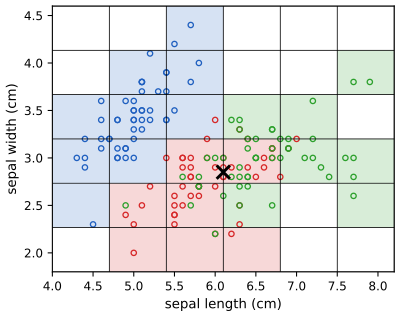
fig_6_2. Download: PDF · SVG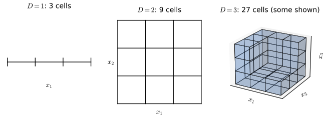
fig_6_3. Download: PDF · SVGFilling the gap 6.2: how many training points the grid classifier needs pp. 174–175
The book says that exponentially many cells need exponentially many training points. Here is the quantitative version, for \(N\) training points that fall into the \(k^D\) cells independently and uniformly (the most favourable case; clustered data leave even more cells empty).
Derivation
Let \(p=k^{-D}\) be the probability of one cell. A given cell is empty with probability \((1-p)^N\), so by linearity of expectation the expected fraction of empty cells is \((1-p)^N\), and a fresh test point (independent of the training set) lands in an empty cell with the same probability \((1-p)^N\).
Lower bound. By Bernoulli's inequality \((1-p)^N\ge1-Np\). So if \(N\le k^D/2\), at least half of all test points cannot be classified, whatever the data.
Upper bound. Since \(1-p\le e^{-p}\), \((1-p)^N\le e^{-Np}\). To make the failure probability at most \(\delta\) it suffices that \(N\ge k^D\ln(1/\delta)\).
Both bounds are of order \(k^D\): the number of training points must grow exponentially with \(D\). With \(k=8\) and \(N=150\) (the size of the Iris data), the fraction of empty cells is 0.75 already for \(D=3\) and 0.995 for \(D=5\). For the Iris data with all four measurements and \(k=8\), the geometry demo shows that most flowers are alone in their cell. ∎
6.1.2 High-dimensional spaces
pp. 175–176 Since the volume of a ball of radius \(r\) in \(\R^D\) scales as \(r^D\),
\[ V_D(r)=K_Dr^D, \tag{6.4} \]the fraction of the unit ball's volume between radius \(1-\epsilon\) and 1 is
\[ \frac{V_D(1)-V_D(1-\epsilon)}{V_D(1)}=1-(1-\epsilon)^D , \tag{6.5} \]which tends to 1 as \(D\to\infty\) for every fixed \(\epsilon\in(0,1]\) (Figure 6.4): almost all of a high-dimensional ball is close to its surface. The same happens to probability mass (Figure 6.5).
Result 6.1 (volumes, corners and the Gaussian shell; Exercises 6.1–6.3) pp. 175–176, (6.4)–(6.5), (6.51)–(6.59)
(1) The unit sphere in \(\R^D\) has surface area and the unit ball volume
\[ S_D=\frac{2\pi^{D/2}}{\Gamma(D/2)},\tag{6.53} \] \[ V_D=\frac{S_D}{D}. \tag{6.54} \](2) A ball of radius \(a\) occupies a fraction
\[ \frac{\text{volume of ball}}{\text{volume of cube}}=\frac{\pi^{D/2}}{D\,2^{D-1}\,\Gamma(D/2)} \tag{6.55} \]of the cube of side \(2a\) around it; this tends to 0 like \((\pi e/2D)^{D/2}/\sqrt{\pi D}\). The corners are at distance \(a\sqrt D\) from the centre, the faces at distance \(a\).
(3) If \(\x\sim\N(\mathbf 0,\sigma^2\I_D)\), the radius \(r=\|\x\|\) has density
\[ p(r)=\frac{S_D\,r^{D-1}}{(2\pi\sigma^2)^{D/2}}\exp\Big(-\frac{r^2}{2\sigma^2}\Big), \tag{6.58} \]with a single maximum at \(\hat r\)
The density of \(\x\) at the origin is \(e^{(D-1)/2}\simeq e^{D/2}\) times its value on the sphere \(\|\x\|=\hat r\): the mass is where the density is not.
Erratum. The book prints (6.59) with the exponent \(-3\epsilon^2/2\sigma^2\) (as did Bishop 2006, whose errata correct it); the second derivative of \(\ln p\) at \(\hat r\) is \(-2/\sigma^2\), which gives \(-\epsilon^2/\sigma^2\). For \(D=1000\) and \(\epsilon=1\), \(p(\hat r+\epsilon)/p(\hat r)=0.372\), against \(e^{-1}=0.368\) and \(e^{-1.5}=0.223\).
Proof
(1) The integral of \(e^{-\|\x\|^2}\) over \(\R^D\) factorises in Cartesian coordinates; in polar coordinates the integrand depends only on \(r\), and the shell between \(r\) and \(r+\d r\) has volume \(S_Dr^{D-1}\d r\). Hence
\[ \prod_{i=1}^{D}\int_{-\infty}^{\infty}e^{-x_i^2}\d x_i=S_D\int_0^\infty e^{-r^2}r^{D-1}\d r. \tag{6.51} \]Each factor on the left is \(\sqrt\pi\), so the left side is \(\pi^{D/2}\). On the right substitute \(u=r^2\), \(\d r=\d u/(2\sqrt u)\):
\[ S_D\int_0^\infty e^{-r^2}r^{D-1}\d r=\frac{S_D}{2}\int_0^\infty e^{-u}u^{D/2-1}\d u=\frac{S_D}{2}\Gamma(D/2), \]using the definition \(\Gamma(x)\)
(2) The ball of radius \(a\) has volume \(V_Da^D\) and the cube \((2a)^D\); the ratio is \(2\pi^{D/2}/(D\,2^D\Gamma(D/2))\), which is (6.55). Stirling's formula \(\Gamma(x)\)
The corner \((a,\dots,a)\) is at distance \(\sqrt{Da^2}=a\sqrt D\) from the centre; the centre of a face is at distance \(a\). The ratio \(\sqrt D\to\infty\): in high dimensions a cube is mostly "spikes" toward its \(2^D\) corners, which the ball misses.
(3) The density \((2\pi\sigma^2)^{-D/2}e^{-r^2/2\sigma^2}\) is constant on spheres, and the shell \([r,r+\epsilon]\) has volume \(S_Dr^{D-1}\epsilon+O(\epsilon^2)\), so its probability is \(p(r)\epsilon+O(\epsilon^2)\) with (6.58). Then \(\ln p(r)\)
See also: Result 1.13 and Result 1.14 in the companion course (the same results for Bishop 2006, Exercises 1.18–1.20).
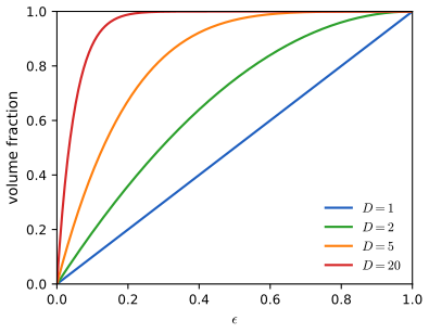
fig_6_4. Download: PDF · SVG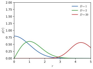
fig_6_5. Download: PDF · SVGFilling the gap 6.3: why the shell is thin, and why distances concentrate p. 176
Result 6.1 locates the peak of \(p(r)\); here is why its width stays of order \(\sigma\) while its location grows like \(\sqrt D\), and the same mechanism for distances between random points, which makes nearest-neighbour ideas fragile in high dimensions.
Derivation
Norms. With \(\x\sim\N(\mathbf 0,\sigma^2\I_D)\), \(r^2=\sum_ix_i^2\) is a sum of \(D\) independent terms with mean \(\sigma^2\) and variance \(\E[x^4]-\sigma^4=2\sigma^4\). So \(\E[r^2]=D\sigma^2\) and \(\var(r^2)=2D\sigma^4\). Chebyshev's inequality gives, for any \(t>0\),
\[ \Pr\Big(\Big|\frac{r^2}{D\sigma^2}-1\Big|\ge t\Big)\le\frac{2}{Dt^2}, \]so \(r/\sqrt D\to\sigma\) in probability. For the spread of \(r\) itself: \(r^2-D\sigma^2\)
Distances. Let \(\x,\x'\) be independent and uniform on \([0,1]^D\). Then \(\|\x-\x'\|^2=\sum_i(x_i-x_i')^2\) is a sum of \(D\) independent copies of \(U=(x-x')^2\), with \(\E U=1/6\) and \(\var U\)
High dimension is not only a curse. In Figure 6.6 two classes that overlap completely when only \(x_1\) is observed become linearly separable once \(x_2\) is added: more features can make a problem easier, as long as the model can exploit them without needing a cell for every combination.
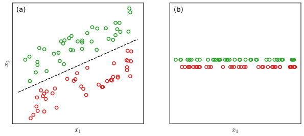
fig_6_6. Download: PDF · SVG6.1.3 Data manifolds
pp. 176–178 Learning in high dimensions is possible because real data do not fill the space. An image of one object, moved horizontally and vertically and rotated, is a point of \(\R^{\text{pixels}}\) that depends smoothly on three numbers \((\Delta x,\Delta y,\theta)\): the set of such images is (approximately) a three-dimensional manifold, however many pixels there are (Figure 6.7). Basis functions that only need to cover the manifold need a number that grows with its dimension \(d\), not with \(D\): covering a \(d\)-dimensional region at resolution \(\varepsilon\) takes of order \(\varepsilon^{-d}\) cells. A learned representation can do better still by ignoring the directions on the manifold that are irrelevant to the task (for orientation, \(\Delta x\) and \(\Delta y\)).

fig_6_7. Download: PDF · SVGA second way to see that data occupy a tiny part of the space is to sample from the whole space: images with independent uniform pixels look nothing like real images (Figure 6.8), because real images have strong correlations between neighbouring pixels.
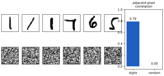
fig_6_8. Download: PDF · SVGErratum (p. 178): "two adjacent images in the random examples" should read "two adjacent pixels".
See also: data near a low-dimensional manifold and Section 12.4.3, modelling nonlinear manifolds, in the companion course.
6.1.4 Data-dependent basis functions
pp. 178–179 Hand-crafted features were the norm before deep learning; the alternative is to let the data choose the basis functions. Placing one basis function on each training point automatically follows the data manifold, for instance the radial basis functions (Broomhead and Lowe 1988)
\[ \phi_n(\x)=\exp\Big(-\frac{\|\x-\x_n\|^2}{s^2}\Big), \tag{6.6} \]but then the model has \(N\) parameters, costs \(O(N^2)\) or more to fit, and needs strong regularisation. Support vector machines (Vapnik 1995) keep a data-chosen subset of the \(\phi_n\), but the subset still grows with \(N\), the outputs are not probabilities, and more than two classes need extra machinery. Neural networks instead give the basis functions their own parameters and learn them, which scales to very large data sets and, with many layers, learns hierarchical representations.
See also: Section 6.3, radial basis function networks, and Section 7.1, support vector machines, in the companion course.
6.2 Multilayer Networks
pp. 180–186 The key idea of neural networks: keep the form (6.1), but give the basis functions their own adjustable parameters and train everything together by gradient-based optimisation of one error function. The choice that has worked best is to make each basis function itself of the form (6.1), a nonlinearity applied to a linear combination of the inputs; repeating this construction gives deep networks.
Definition 6.1 (two-layer network) pp. 180–181, (6.7)–(6.9)
A network with \(D\) inputs, \(M\) hidden units and \(K\) outputs computes the pre-activations and hidden-unit outputs
\[ a^{(1)}_j=\sum_{i=1}^{D}w^{(1)}_{ji}x_i+w^{(1)}_{j0}, \tag{6.7} \] \[ z^{(1)}_j=h\big(a^{(1)}_j\big),\qquad j=1,\dots,M, \tag{6.8} \]where the activation function \(h\) is differentiable (almost everywhere, for ReLU) and nonlinear, then the output pre-activations
\[ a^{(2)}_k=\sum_{j=1}^{M}w^{(2)}_{kj}z^{(1)}_j+w^{(2)}_{k0},\qquad k=1,\dots,K, \tag{6.9} \]and the outputs \(y_k=f(a^{(2)}_k)\) with an output activation \(f\) (identity, logistic sigmoid or softmax, Section 6.4). The \(w_{ji}\) are weights, the \(w_{j0}\) biases; there are \(W=M(D+1)+K(M+1)\) parameters. The book calls this a two-layer network because it has two layers of learnable weights (it is also called a three-layer network, counting layers of units, or a single-hidden-layer network).
See also: Definition 5.1 in the companion course.
6.2.1 Parameter matrices
p. 181 With an extra input \(x_0=1\) the bias joins the weights,
\[ a_j=\sum_{i=0}^{D}w^{(1)}_{ji}x_i, \tag{6.10} \]and with \(z_0=1\) the whole network is
\[ y_k(\x,\w)=f\Big(\sum_{j=0}^{M}w^{(2)}_{kj}\,h\Big(\sum_{i=0}^{D}w^{(1)}_{ji}x_i\Big)\Big), \tag{6.11} \]or, with \(f\) and \(h\) acting elementwise,
\[ \y(\x,\w)=f\big(\W^{(2)}h\big(\W^{(1)}\x\big)\big). \tag{6.12} \]Erratum (p. 181): the input vector is \(\x=(x_1,\dots,x_D)^\T\), not \((x_1,\dots,x_N)^\T\).
Filling the gap 6.4: what (6.12) means exactly, and its gradient in matrix form p. 181
(6.12) silently re-appends the constant 1 after the hidden layer. Written out, the forward pass and its gradient (derived in general in Chapter 8) take three lines each.
Derivation
Forward pass. Let \(\tilde\x\)
which is (6.11) in matrix form; (6.12) is shorthand for this.
Gradient. Take one pattern with error \(E_n\), and suppose the output error signal \(\bm\delta^{(2)}\)
In matrices, with \(\bar\W^{(2)}\) the matrix \(\W^{(2)}\) without its bias column and \(\odot\) the elementwise product:
\[ \frac{\partial E_n}{\partial\W^{(2)}}=\bm\delta^{(2)}\tilde\z^\T,\qquad \bm\delta^{(1)}=h'(\mathbf a^{(1)})\odot\big(\bar\W^{(2)\T}\bm\delta^{(2)}\big),\qquad \frac{\partial E_n}{\partial\W^{(1)}}=\bm\delta^{(1)}\tilde\x^\T . \]For a batch, stack the patterns as rows: \(\partial E/\partial\W^{(2)}\)TwoLayer.backward is exactly these lines, and it agrees with finite differences. ∎
See also: Result 5.6, the backpropagation formulae, in the companion course.
6.2.2 Universal approximation
pp. 181–182 Figure 6.10 shows a network with only three tanh hidden units fitting four quite different functions; each hidden unit contributes a smooth step, and the output layer adds and scales them. Figure 6.11 shows the same idea for classification: the two hidden units define two lines, and the output unit combines them into a bent decision boundary close to the optimal one.
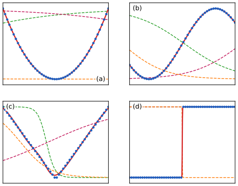
fig_6_10. Download: PDF · SVG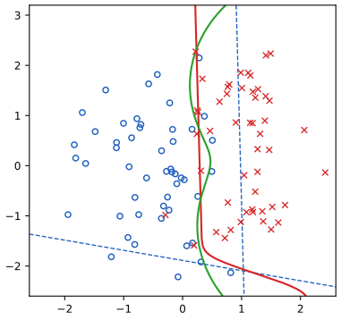
fig_6_11. Download: PDF · SVGThe book cites the theorems of the late 1980s (Funahashi 1989; Cybenko 1989; Hornik, Stinchcombe and White 1989) and the sharp form of Leshno et al. (1993) without stating them. Here is the precise statement and a complete, elementary proof for the activation functions of this chapter.
Result 6.2 (universal approximation) p. 182
Let \(h:\R\to\R\) be continuous and \(\mathcal K\subset\R^D\) compact. The functions
\[ g(\x)=v_0+\sum_{j=1}^{M}v_j\,h\big(\w_j^\T\x+b_j\big),\qquad M\in\{1,2,\dots\},\ v_j,b_j\in\R,\ \w_j\in\R^D, \](two-layer networks with one linear output) are dense in \(C(\mathcal K)\): for every continuous \(f\) on \(\mathcal K\) and every \(\varepsilon>0\) there is such a \(g\) with \(\sup_{\x\in\mathcal K}|f(\x)-g(\x)|<\varepsilon\), if and only if \(h\) is not a polynomial (Leshno et al. 1993). Below, "if" is proved for every activation of Figure 6.12 and for the logistic sigmoid and swish, and "only if" in general. Vector outputs follow by approximating each output separately.
The theorem says nothing about how large \(M\) must be (in general it can grow exponentially with \(D\)), nor whether training will find the weights.
Proof
Step 0: reductions. If \(h\) is replaced by \(\alpha h(\beta u+\gamma)+\delta\) with \(\alpha,\beta\ne0\), the class of networks is unchanged (absorb \(\beta,\gamma\) into \(\w_j,b_j\), \(\alpha\) into \(v_j\), \(\delta\) into \(v_0\)). So tanh \(=2\sigma(2u)-1\) (Result 6.3) and hard tanh \(=2\,\mathrm{ramp}-1\) behave like sigmoidal functions (continuous, with limits 0 at \(-\infty\) and 1 at \(+\infty\) after rescaling). A ReLU can be built exactly from two leaky ReLUs (\(\mathrm{lrelu}\) with slope \(\alpha\)),
\[ \relu(u)=\frac{1}{1-\alpha}\Big(\mathrm{lrelu}(u)-\frac{\alpha}{1+\alpha}\big(\mathrm{lrelu}(u)-\mathrm{lrelu}(-u)\big)\Big), \]and on a bounded set \(|u|\le c\) from three absolute values, \(\relu(u)\)
Step 1: one input, sigmoidal \(h\). Let \(\psi\) be continuous on \([a,b]\) with modulus of continuity \(\omega(\delta)\)
which is below any \(\varepsilon\) once \(n\) is large enough to make \(\omega(\ell)\) small and then \(s\) is large enough. For the logistic sigmoid \(\eta(s)\le e^{-s\ell/4}\), and for Lipschitz \(\psi\) the error is \(O(1/n)\).
Step 2: one input, ReLU. The piecewise-linear interpolant of \(\psi\) at the knots \(u_0,\dots,u_n\) is exactly a ReLU network with \(n\) hidden units:
\[ g(u)=\psi(u_0)+\sum_{j=1}^{n}(s_j-s_{j-1})\relu(u-u_{j-1}),\qquad s_j=\frac{\psi(u_j)-\psi(u_{j-1})}{\ell},\ s_0=0, \]since on \([u_{i-1},u_i]\) its slope is \(\sum_{j\le i}(s_j-s_{j-1})=s_i\) and \(g(u_0)=\psi(u_0)\). On each interval \(g\) lies between \(\psi(u_{i-1})\) and \(\psi(u_i)\), so \(|g-\psi|\le\omega(\ell)\); if \(\psi\in C^2\), the interpolation error formula \(\psi(u)-g(u)\)
Step 3: any dimension. Let \(\mathcal T\) be the set of finite sums \(\sum_mc_m\cos(\bm\omega_m^\T\x+\phi_m)\) restricted to \(\mathcal K\). It is a real algebra of continuous functions (closed under sums, scalar multiples and products, since \(\cos A\cos B\)
Step 4: "only if". If \(h\) is a polynomial of degree \(p\), every hidden unit \(h(\w_j^\T\x+b_j)\), and hence every network, is a polynomial in \(\x\) of degree at most \(p\). These form a finite-dimensional, hence closed, subspace of \(C(\mathcal K)\), which for \(\mathcal K=[0,1]^D\) does not contain \(x_1^{p+1}\); a closed proper subspace is not dense. ∎
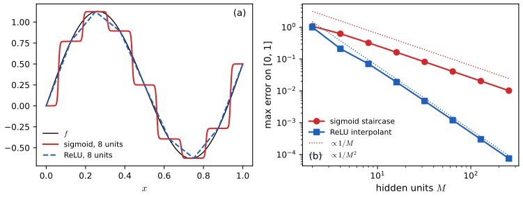
fig_approx_rate. Download: PDF · SVGHow many hidden units? In Step 3 the count is (number of Fourier terms) × (units per term), and for a general Lipschitz function on \([0,1]^D\) a grid-type construction needs of order \(\varepsilon^{-D}\) units: the curse of dimensionality returns. For smoother classes it does not: if \(f\) has a Fourier transform with \(C_f\)
See also: Result 5.1 (universal approximation, one-dimensional proof) and the backpropagation demo in the companion course.
6.2.3 Hidden unit activation functions
pp. 182–185 The output activation is dictated by the distribution being modelled (Section 6.4); for hidden units the only requirement is differentiability. Usually all hidden units share one activation.
Linear hidden units add nothing: a composition of linear maps is linear. Worse, with fewer hidden units than inputs or outputs they restrict the map.
Filling the gap 6.5: linear hidden units, bottlenecks and rank p. 183
Derivation
With \(h(a)=a\) and no biases, \(\y=\W^{(2)}\W^{(1)}\x\) with \(\W^{(1)}\in\R^{M\times N}\), \(\W^{(2)}\in\R^{K\times M}\) (\(N\) inputs, as on p. 183). The network uses \(M(N+K)\) parameters and computes the single linear map \(\mathbf A\)
See also: Filling the gap 5.1 and Section 12.4.2, autoassociative networks, in the companion course.
The classical nonlinear choices are the logistic sigmoid and tanh,
\[ \sigma(a)=\frac{1}{1+\exp(-a)}, \tag{6.13} \] \[ \tanh(a)=\frac{e^a-e^{-a}}{e^a+e^{-a}}, \tag{6.14} \]and their piecewise-linear and unbounded relatives: hard tanh (Collobert 2004), softplus, the rectified linear unit and the leaky ReLU,
\[ h(a)=\max(-1,\min(1,a)), \tag{6.15} \] \[ h(a)=\ln(1+\exp(a)), \tag{6.16} \] \[ h(a)=\max(0,a), \tag{6.17} \] \[ h(a)=\max(0,a)+\alpha\min(0,a),\qquad 0<\alpha<1, \tag{6.18} \]with \(\alpha=-1\) giving \(|a|\), and a learnable \(\alpha_j\) per unit giving the parametric ReLU (Figure 6.12). The ReLU is the usual default: it trains deep networks much faster than sigmoidal units (Krizhevsky et al. 2012), is cheap and works in low precision.
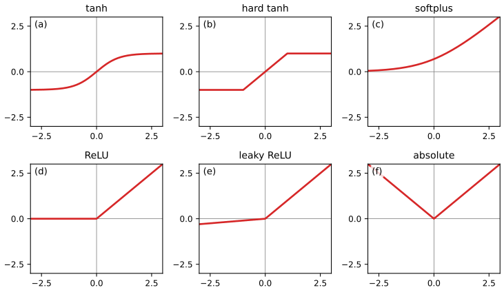
fig_6_12. Download: PDF · SVGResult 6.3 (activation functions: identities and derivatives; Exercises 6.4–6.7) pp. 183–185, (6.13)–(6.18), (6.60)–(6.65)
(1) \(\sigma'(a)=\sigma(a)\{1-\sigma(a)\}\), \(\tanh(a)=2\sigma(2a)-1\) and \(\tanh'(a)=1-\tanh^2(a)\).
(2) A two-layer network with logistic-sigmoid hidden units computes exactly the same function as the tanh network with
\[ \tilde w^{(1)}_{ji}=\tfrac12w^{(1)}_{ji}\ (i=0,\dots,D),\qquad \tilde w^{(2)}_{kj}=\tfrac12w^{(2)}_{kj}\ (j\ge1),\qquad \tilde w^{(2)}_{k0}=w^{(2)}_{k0}+\tfrac12\sum_{j=1}^{M}w^{(2)}_{kj}, \]an invertible linear map of the parameters (so the two families of networks coincide, although training from the same initial weights does not).
(3) The softplus \(\zeta(a)=\ln(1+e^a)\) satisfies \(\zeta(a)-\zeta(-a)=a\) (6.62), \(\ln\sigma(a)=-\zeta(-a)\) (6.63), \(\zeta'(a)=\sigma(a)\) (6.64) and, for \(a>0\), \(\zeta^{-1}(a)=\ln(e^a-1)\) (6.65); moreover \(0<\zeta(a)-\relu(a)\le\ln2\).
(4) Swish \(h_\beta(x)=x\,\sigma(\beta x)\) (6.61) has derivative \(\sigma(\beta x)+\beta x\,\sigma(\beta x)\{1-\sigma(\beta x)\}\); it tends to \(\relu(x)\) uniformly as \(\beta\to\infty\), with \(\sup_x|h_\beta(x)-\relu(x)|\)
Proof
(1) \(\sigma'(a)\)
(2) By (1), \(\sigma(a)=\tfrac12\{1+\tanh(a/2)\}\). So
\[ \sum_{j=1}^Mw^{(2)}_{kj}\sigma(a_j)+w^{(2)}_{k0}=\sum_{j=1}^M\tfrac12w^{(2)}_{kj}\tanh(a_j/2)+w^{(2)}_{k0}+\tfrac12\sum_{j=1}^Mw^{(2)}_{kj}, \]and \(a_j/2\)
(3) \(\zeta(a)-\zeta(-a)\)
(4) The derivative is the product rule with \(\sigma'=\sigma(1-\sigma)\). For the limit see Filling the gap 6.7; as \(\beta\to0\), \(\sigma(\beta x)\to\tfrac12\) uniformly on bounded sets. ∎
See also: Filling the gap 5.2 (tanh and logistic units are equivalent) in the companion course.
Filling the gap 6.6: why sigmoidal units saturate, and why ReLUs die pp. 184–185
The book says that the gradients of sigmoid and tanh "go to zero exponentially" for large inputs, and that ReLU units may receive no error signal. Both statements are about \(h'\) in the gradient \(\partial E_n/\partial w^{(1)}_{ji}\)
Derivation
Exponential decay. \(\sigma'(a)\)
Dead ReLUs. For the ReLU, \(h'(a)=1\) for \(a>0\) and 0 for \(a<0\). If \(a_j(\x_n)<0\) for every training input, then \(\partial E/\partial w^{(1)}_{ji}=0\) for all \(i\) (including the bias) and \(\partial E/\partial w^{(2)}_{kj}\)
Scale. The ReLU is positively homogeneous, \(\relu(ca)=c\,\relu(a)\) for \(c>0\), so rescaling a unit's input weights rescales its output without changing where it is active: its behaviour does not depend on staying in a narrow "linear" range, which is one reason it is less sensitive to initialisation. How these effects compound through many layers is the subject of Section 7.4. ∎
Filling the gap 6.7: how fast swish becomes a ReLU (Exercise 6.5) p. 205
Derivation
For \(x\ge0\), \(\relu(x)-x\sigma(\beta x)\)
\(\varphi(0)=0\), \(\varphi(u)\to0\) as \(u\to\infty\), and \(\varphi'(u)\)
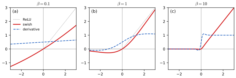
fig_ex6_5. Download: PDF · SVG6.2.4 Weight-space symmetries
pp. 185–186 Many weight vectors give the same network function (Chen, Lu and Hecht-Nielsen 1993). For tanh units, flipping the signs of all weights into and out of one hidden unit, or swapping two hidden units together with their weights, leaves the function unchanged; the book counts \(M!\,2^M\) equivalent weight vectors and states that these are all the symmetries (apart from accidental ones), and that the phenomenon is not special to tanh (Kůrková and Kainen 1994).
Result 6.4 (weight-space symmetries) pp. 185–186
Consider a two-layer network with \(M\) hidden units; write \(\mathbf u_j\)
(1) For any \(h\), permuting the hidden units (moving \((\mathbf u_j,\mathbf v_j)\) to position \(\pi(j)\)) preserves the function. If \(h\) is odd, so does each sign flip \((\mathbf u_j,\mathbf v_j)\mapsto(-\mathbf u_j,-\mathbf v_j)\). The signed permutations form a group of order \(M!\,2^M\).
(2) If every \(\mathbf u_j\ne\mathbf 0\) and \(\mathbf u_i\ne\pm\mathbf u_j\) for \(i\ne j\) (true for almost every weight vector), the \(M!\,2^M\) transformed weight vectors are all different. With several hidden layers the factors multiply, one per layer.
(3) For tanh, these are the only symmetries of a minimal network (Sussmann 1992; Chen et al. 1993): if two irreducible networks with the same number of units compute the same function, one is a signed permutation of the other.
(4) For the ReLU, which is not odd, sign flips change the function in general; instead positive rescaling \((\mathbf u_j,\mathbf v_j)\mapsto(c\,\mathbf u_j,\mathbf v_j/c)\), \(c>0\), preserves it. So every weight vector of a ReLU network has a continuum (an \(M\)-dimensional family) of equivalent weight vectors, and the count \(M!\,2^M\) does not apply.
Proof
(1) The output pre-activation is \(a_k\)
(2) Suppose \((\pi,\mathbf s)\) and \((\pi',\mathbf s')\) produce the same weight vector. Looking at position \(\pi(j)=\pi'(j')\), \(s_j\mathbf u_j=s'_{j'}\mathbf u_{j'}\); by the assumption this forces \(j=j'\), so \(\pi=\pi'\), and then \(s_j\mathbf u_j=s'_j\mathbf u_j\) with \(\mathbf u_j\ne\mathbf 0\) forces \(s_j=s'_j\). So the orbit has exactly \(M!\,2^M\) elements (listing all 48 for \(M=3\) gives outputs equal to \(10^{-15}\)).
(3), sketch for one input and one output. \(g(x)=v_0+\sum_jv_j\tanh(w_jx+b_j)\) extends to a meromorphic function of complex \(x\). Since \(\tanh\) has simple poles at \(i\pi(k+\tfrac12)\), \(k\in\mathbb Z\), each with residue 1, unit \(j\) contributes poles at \(x=(i\pi(k+\tfrac12)-b_j)/w_j\) with residues \(v_j/w_j\). These lie on a vertical line at real part \(-b_j/w_j\), spaced by \(\pi/|w_j|\), so the pole set determines \((w_j,b_j)\) up to a common sign, and the residue then fixes \(v_j\) with the matching sign. Distinct units (\((w_i,b_i)\ne\pm(w_j,b_j)\)) have disjoint pole sets, so no poles cancel; equal functions have equal poles and residues, so the units agree up to order and sign. The general case is Sussmann's theorem.
(4) \(\relu(ca)=c\,\relu(a)\) for \(c>0\), so \((w^{(2)}_{kj}/c)\relu(c\,\mathbf u_j^\T\tilde\x)\)
The symmetries matter little for finding a good weight vector, but they do in Bayesian treatments: a posterior over weights has \(M!\,2^M\) equivalent modes, a factor that enters the evidence when networks of different sizes are compared (Bishop 2006, Section 5.7).
See also: Result 5.2 (sign-flip and interchange symmetries) in the companion course.
6.3 Deep Networks
pp. 186–194 For decades the two-layer network was the standard architecture, mainly because deeper ones were hard to train (Chapter 7 explains what changed). The extension to \(L\) layers is immediate.
Definition 6.2 (deep network) pp. 186–187, (6.19)
With \(\z^{(0)}=\x\), layer \(l=1,\dots,L\) computes
\[ \z^{(l)}=h^{(l)}\big(\W^{(l)}\z^{(l-1)}\big), \tag{6.19} \]where \(\W^{(l)}\in\R^{n_l\times(n_{l-1}+1)}\) holds the weights and biases of layer \(l\) (acting on \(\z^{(l-1)}\) with a 1 appended, as in Filling the gap 6.4), \(h^{(l)}\) acts elementwise, and \(\y=\z^{(L)}\) (so \(h^{(L)}\) is the output activation). The network has \(L\) layers of learnable weights and \(\sum_{l=1}^{L}n_l(n_{l-1}+1)\) parameters.
Two-layer networks are already universal (Result 6.2), so why go deeper? The book gives two reasons. The first is efficiency: Montúfar et al. (2014) showed that a ReLU network divides its input space into a number of linear regions that can grow exponentially with depth but only polynomially with width, so some functions computed by deep networks need exponentially many units in a shallow one. The two results below make this precise and prove the cleanest case.
Result 6.5 (linear regions of ReLU networks; one hidden layer) p. 187
(1) A network whose hidden units are ReLUs (any depth, linear output) is a continuous function that is affine on each set of inputs sharing one activation pattern (the list of which units are on). Its linear regions are the maximal connected sets on which it is affine.
(2) With one hidden layer of \(M\) units on \(\R^D\), the hyperplanes \(\{\x:\w_j^\T\x+b_j=0\}\) cut \(\R^D\) into at most
\[ r(M,D)=\sum_{j=0}^{D}\binom{M}{j} \]regions, with equality when the hyperplanes are in general position; each region has its own activation pattern, and the network has at most \(r(M,D)\) linear regions. For \(D=1\): at most \(M+1\) pieces; for \(D=2\): at most \(1+M+\binom M2\).
(3) In a bounded convex region of the plane, for lines in general position (no three through a point, no crossing on the boundary), the number of regions is 1 plus the number of lines that enter it plus the number of crossings inside it.
Proof
(1) Fix an activation pattern and the set \(S\) of inputs that produce it. On \(S\), the first layer's pre-activations are affine in \(\x\), and each ReLU either returns its (affine) input or 0, so \(\z^{(1)}\) is affine on \(S\); by induction every layer, and the output, is affine on \(S\). Continuity holds because compositions of continuous functions are continuous.
(2) For one layer the pattern of \(\x\) is the vector of signs of \(\w_j^\T\x+b_j\), so the sets of constant pattern are exactly the regions of the hyperplane arrangement (distinct regions have distinct sign vectors). Let \(r(M,D)\) be the maximum number of regions of \(M\) hyperplanes in \(\R^D\). Add the \(M\)th hyperplane \(H\) to an arrangement of \(M-1\). Each region that \(H\) passes through is split into two, and the parts of \(H\) inside those regions are the regions of the arrangement that the other \(M-1\) hyperplanes induce on \(H\cong\R^{D-1}\); there are at most \(r(M-1,D-1)\) of them. Hence
\[ r(M,D)\le r(M-1,D)+r(M-1,D-1),\qquad r(0,D)=1,\quad r(M,0)=1, \]with equality in general position (the induced arrangement on \(H\) is again in general position). The right side \(\sum_{j\le D}\binom Mj\) satisfies the same recursion by Pascal's rule \(\binom Mj=\binom{M-1}j+\binom{M-1}{j-1}\) and the same boundary values, so it is the solution. The network is affine on each region, so it has at most this many linear regions (fewer if two neighbouring regions happen to carry the same affine function, for example when an output weight is 0).
(3) Add the lines one at a time. A line that enters the region and crosses \(c\) earlier lines inside it is cut into \(c+1\) segments, each of which splits one existing region in two, so it adds \(c+1\) regions. Summing over the lines gives \(1+\sum_i(c_i+1)\)
Result 6.6 (depth separation: the sawtooth) p. 187
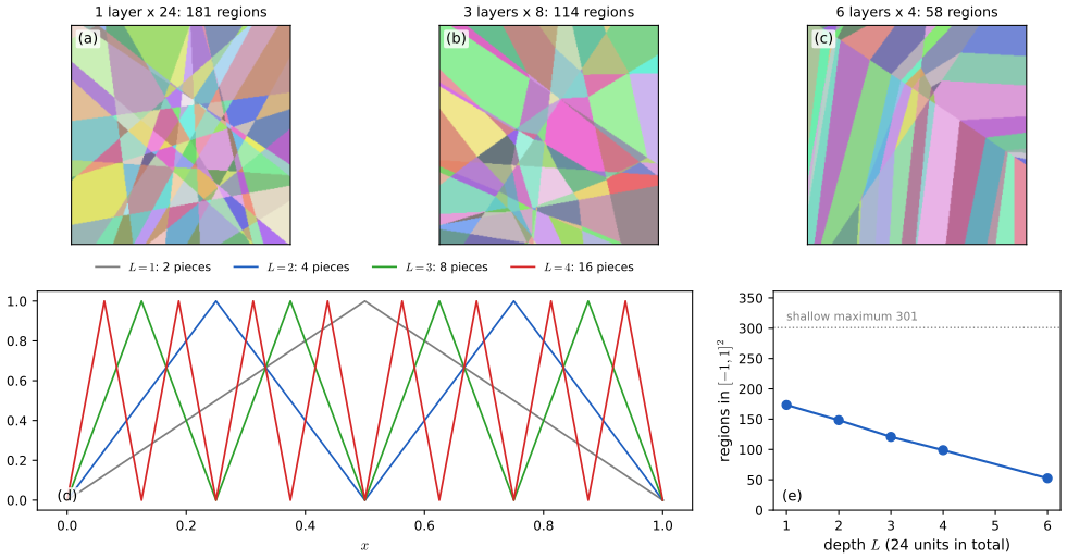
Let \(g(x)=2\relu(x)-4\relu(x-\tfrac12)\) (the tent map on \([0,1]\)). The \(L\)-fold composition \(g^{\circ L}=g\circ\dots\circ g\) is a ReLU network with \(L\) hidden layers of 2 units, and on \([0,1]\) it has exactly \(2^L\) linear pieces. A ReLU network with one hidden layer of \(M\) units on \(\R\) has at most \(M+1\) pieces, so it needs \(M\ge2^L-1\) units to represent \(g^{\circ L}\). More generally, a ReLU network on \(\R\) with \(k\) hidden layers of width \(n\) has at most \((n+1)^k\) pieces, so representing \(g^{\circ L}\) with \(k\) layers requires \(n\ge2^{L/k}-1\).
Proof
The tent. On \([0,\tfrac12]\), \(g(x)=2x\); on \([\tfrac12,1]\), \(g(x)=2x-4(x-\tfrac12)=2-2x\). So \(g\) maps each half of \([0,1]\) linearly and bijectively onto \([0,1]\).
Claim: on each interval \(I_k=[k2^{-L},(k+1)2^{-L}]\), \(k=0,\dots,2^L-1\), \(g^{\circ L}\) is affine with slope \(\pm2^L\) and maps \(I_k\) onto \([0,1]\). True for \(L=1\). If it holds for \(L-1\), each \(I_k\) of level \(L-1\) is mapped linearly onto \([0,1]\) by \(g^{\circ(L-1)}\); its two halves (the intervals of level \(L\)) are mapped onto \([0,\tfrac12]\) and \([\tfrac12,1]\), and \(g\) maps each of these linearly onto \([0,1]\) with slope \(\pm2\). The slopes alternate in sign between neighbouring intervals (the function goes up to 1 and back down to 0), so no two neighbours merge: exactly \(2^L\) pieces.
As a network. Layer \(l\) has the two units \(\relu(u)\), \(\relu(u-\tfrac12)\) where \(u\) is the previous layer's output \(2z_1-4z_2\) (the input \(x\) for \(l=1\)); the combination \(2z_1-4z_2\) is folded into the next layer's weights, which is (6.19) with 2 units per layer.
Upper bound for shallow networks. \(f(x)=v_0+\sum_{j=1}^Mv_j\relu(w_jx+b_j)\) can change slope only at the points \(x=-b_j/w_j\) (\(w_j\ne0\)), at most \(M\) of them, so it has at most \(M+1\) pieces. For \(k\) layers: if the input to a layer is piecewise linear with \(P\) pieces, each of its \(n\) units \(\relu(\text{affine combination})\) is affine on each piece except for at most one new breakpoint per piece where its argument crosses 0. The layer's outputs therefore share at most \((P-1)+nP\) breakpoints, i.e. at most \((n+1)P\) pieces. Starting from \(P=1\) gives \((n+1)^k\). Setting \((n+1)^k\ge2^L\) gives the bound. ∎
The general picture (Montúfar et al. 2014), sketch. For \(L\) hidden layers of width \(n\ge D\) on \(\R^D\), the maximal number of linear regions is at least \(\lfloor n/D\rfloor^{D(L-1)}\sum_{j=0}^{D}\binom nj\). The construction generalises the tent: in each of the first \(L-1\) layers, \(D\) groups of \(\lfloor n/D\rfloor\) units each fold one coordinate's interval \(\lfloor n/D\rfloor\) times onto itself, so the layer maps \(\lfloor n/D\rfloor^D\) disjoint cubes onto one cube; the last layer's arrangement (\(\sum_j\binom nj\) regions of the cube) is then replicated in each of the \(\lfloor n/D\rfloor^{D(L-1)}\) preimages. A single layer with the same \(nL\) units has at most \(\sum_{j\le D}\binom{nL}{j}=O((nL)^D)\) regions: polynomial against exponential in \(L\).
But random networks do not reach it. The maximum is a statement about special weights. At a standard random initialisation the number of regions grows roughly with the total number of units, not exponentially with depth (Hanin and Rolnick 2019); in the figure below, with 24 units in total, the average count on \([-1,1]^2\) even falls from 173 (one layer) to 53 (six layers of 4), because narrow random layers often switch off or collapse whole areas. Depth makes exponential complexity possible; training decides whether it is used.
fig_relu_regions. Download: PDF · SVG6.3.1 Hierarchical representations
p. 187 The second, and in practice more important, reason for depth is inductive bias. A deep network composes functions, so it is predisposed to describe its output as built from parts that are themselves built from parts: edges, then shapes such as eyes and whiskers, then a cat. Read generatively, each level combines the components of the level below in many ways, so the number of describable configurations multiplies with each level, the same multiplicative growth as in Result 6.6. Chapter 10 shows such hierarchies emerging in convolutional networks.
6.3.2 Distributed representations
pp. 187–188 If each of \(M\) hidden units signals one feature, a layer can represent \(M\) features; if instead combinations of units are used, the same layer can distinguish up to \(2^M\) on/off patterns. The book's example: "glasses", "hat" and "beard" need 8 units if each combination has its own detector, but only 3 if each unit encodes one attribute. The activation patterns of Result 6.5 are exactly such a distributed code of the input space: \(M\) units, up to \(\sum_{j\le D}\binom Mj\) regions in one layer and far more with depth. (A single linear layer on top of a distributed code cannot, however, compute every Boolean function of the attributes; "exactly one of hat or beard" is XOR, which needs a further hidden layer.)
6.3.3 Representation learning
pp. 188–189 The hidden layers transform the data into a space in which the task becomes easy: for a classifier whose last layer is logistic regression, the classes must be (nearly) linearly separable in the space of the last hidden layer. That space, an embedding, can be computed for any input by forward propagation and reused. Representations can also be learned without labels: an autoencoder is trained to reproduce its input through a narrow hidden layer (Section 19.1), which forces a compressed code; with linear units this is PCA (Filling the gap 6.5). Historically, layer-wise unsupervised pre-training made the first deep networks trainable; later, purely supervised training from scratch was found to work, but large-scale pre-training (for example of transformer language models, Chapter 12) remains central.
See also: Section 12.4.2, autoassociative neural networks, in the companion course.
6.3.4 Transfer learning
pp. 189–191 A representation learned on a data-rich task B (everyday object recognition) can serve a related data-poor task A (skin-lesion classification): copy the early layers and retrain the last one or few on A (Figure 6.13 of the book, a schematic, not reproduced). Two practical remarks follow from the mathematics. First, when only the last layer is retrained, the training inputs can be passed through the frozen layers once and stored, after which each gradient step costs only as much as the small head. Second, if the head is a single softmax or sigmoid layer trained by cross-entropy, the problem in its weights is logistic regression on fixed features, whose error function is convex (its Hessian is a sum of positive semidefinite terms, Chapter 5), so it has no spurious local minima. Fine-tuning instead adapts all layers with a small learning rate for a few iterations, to avoid over-fitting the small data set. Multitask learning (Caruana 1997) trains shared early layers on several tasks at once; meta-learning learns how to learn, enabling few-shot and one-shot learning of new classes (Hospedales et al. 2021).
6.3.5 Contrastive learning
pp. 191–193 Contrastive learning learns an embedding \(f_\w(\x)\), normalised to \(\|f_\w(\x)\|=1\), in which a positive pair \((\x,\x^+)\) is close and negative pairs \((\x,\x^-_n)\) are far apart. The standard loss is InfoNCE (Gutmann and Hyvärinen 2010; Oord, Li and Vinyals 2018):
\[ E(\w)=-\ln\frac{\exp\{f_\w(\x)^\T f_\w(\x^+)\}}{\exp\{f_\w(\x)^\T f_\w(\x^+)\}+\sum_{n=1}^{N}\exp\{f_\w(\x)^\T f_\w(\x^-_n)\}}. \tag{6.20} \]The pairs encode prior knowledge: augmented versions of one image (instance discrimination), two images of the same class (supervised contrastive learning, Khosla et al. 2020), or an image and its caption, embedded by two different networks \(f_\w\) and \(g_\theta\) (CLIP, Radford et al. 2021), with the symmetric loss
\[ E(\w)=-\frac12\ln\frac{e^{f_\w(\x^+)^\T g_\theta(\y^+)}}{e^{f_\w(\x^+)^\T g_\theta(\y^+)}+\sum_{n=1}^{N}e^{f_\w(\x^-_n)^\T g_\theta(\y^+)}}-\frac12\ln\frac{e^{f_\w(\x^+)^\T g_\theta(\y^+)}}{e^{f_\w(\x^+)^\T g_\theta(\y^+)}+\sum_{m=1}^{M}e^{f_\w(\x^+)^\T g_\theta(\y^-_m)}}. \tag{6.21} \]Figure 6.14 of the book (a schematic of the three paradigms) is not reproduced.
Filling the gap 6.8: InfoNCE as a cross-entropy, its gradient, and why the negatives matter pp. 191–192
The book notes that (6.20) "resembles" a classification cross-entropy and that without negatives the embedding would collapse. Both statements can be made exact.
Derivation
Write \(\mathbf f=f_\w(\x)\), \(\mathbf k_0=f_\w(\x^+)\), \(\mathbf k_n=f_\w(\x^-_n)\) and the logits \(s_n=\mathbf f^\T\mathbf k_n\), \(n=0,\dots,N\). Then (6.20) is \(E=-s_0+\ln\sum_{n=0}^Ne^{s_n}\): exactly the softmax cross-entropy (6.36)–(6.37) of an \((N+1)\)-class problem whose logits are the cosine similarities and whose correct class is 0. Likewise (6.21) is the average of two such cross-entropies (image-to-text and text-to-image).
Gradient. With \(p_n=e^{s_n}/\sum_me^{s_m}\), the canonical-link result gives \(\partial E/\partial s_n=p_n-[n=0]\), and since \(\partial s_n/\partial\mathbf f\)
A gradient step moves the anchor toward its positive and away from the negatives, each negative weighted by how similar it currently is ("hard" negatives push hardest). The constraint \(\|\mathbf f\|=1\) is enforced by normalising the network output, which projects this gradient onto the tangent space of the sphere.
Bounds. Since \(E\)
with the minimum attained when \(\mathbf k_0=\mathbf f\) and every \(\mathbf k_n=-\mathbf f\). A collapsed embedding (all vectors equal) gives \(E=\ln(N+1)\), strictly above the minimum, so collapse is penalised. Without the negatives, (6.20) becomes \(-\ln(e^{s_0}/e^{s_0})\equiv0\), which carries no signal at all, and any loss that only rewards \(s_0\) (such as \(-s_0\)) is minimised by the collapsed map \(f_\w\equiv\) const: the degenerate solution the book warns about. In practice the logits are divided by a temperature \(\tau<1\), which lowers the floor to \(\ln(1+Ne^{-2/\tau})\) and sharpens the weights \(p_n\). Numerical tests verify the cross-entropy identity and the gradient against automatic differentiation, and the bounds numerically. ∎
6.3.6 General network architectures
pp. 193–194 Any directed acyclic graph of units defines a network: unit \(k\) computes
\[ z_k=h\Big(\sum_{j\in\mathcal A(k)}w_{kj}z_j+b_k\Big), \tag{6.22} \]where \(\mathcal A(k)\) is the set of units that send a connection to \(k\) (the book calls them ancestors; strictly they are the parents, the immediate predecessors).
Filling the gap 6.9: why "successive application of (6.22)" is well defined p. 193
Derivation
A topological order exists. A finite directed graph without directed cycles has a unit with no incoming connection: otherwise, walking backwards along incoming connections from any unit would never stop, and in a finite graph must revisit a unit, which closes a cycle. Remove such a unit, and repeat: the order of removal lists the units so that every connection goes from an earlier unit to a later one. Inputs (no incoming connections) can be listed first.
Evaluation. Process units in this order: when unit \(k\) is reached, all its parents \(\mathcal A(k)\) have values, so (6.22) gives \(z_k\). Each connection is used once, so a forward pass costs \(O(\text{number of connections})\), and the outputs are deterministic functions of the inputs. With a cycle there would be no such order and (6.22) would be a system of equations with possibly zero or many solutions (as in recurrent networks, Chapter 12, which unroll the cycle in time).
Matrix view. Collect all units in a vector \(\z\) and the weights in a matrix \(\mathbf A\) with \(A_{kj}=w_{kj}\) if \(j\in\mathcal A(k)\). In topological order \(\mathbf A\) is strictly lower triangular, hence nilpotent (\(\mathbf A^n=\mathbf 0\) for \(n\) units), and starting from the inputs the iteration \(\z\leftarrow h(\mathbf A\z+\mathbf b)\) (inputs held fixed) reaches the network's values after at most depth-many sweeps. Numerical tests confirm both evaluations agree for the network of Figure 6.15. ∎
6.3.7 Tensors
p. 194 Data, activations and parameters are often arrays with more than two indices: a batch of \(N\) colour images of \(I\times J\) pixels is a four-index array \(x_{ijkn}\) (row, column, colour channel, image). Such arrays are called tensors (in the computing sense: multi-dimensional arrays, without the transformation rules of the physicist's tensors), and the operations of a network are sums over shared indices, which GPUs execute in parallel. For example a fully connected layer applied to a batch is \(a_{nj}=\sum_iw_{ji}x_{ni}+b_j\), one matrix product for all \(N\) inputs.
6.4 Error Functions
pp. 194–198 As for the linear models of Chapters 4 and 5, the error function is the negative log likelihood of a conditional distribution of the targets, and each distribution comes with a natural output activation (its canonical link).
6.4.1 Regression
pp. 194–196 For a real target with Gaussian noise around the network output,
\[ p(t\given\x,\w)=\N\big(t\given y(\x,\w),\sigma^2\big), \tag{6.23} \]with linear output units (enough, since by Result 6.2 the network can approximate any continuous mean function). For i.i.d. data the likelihood is
\[ p(\tv\given\mathbf X,\w,\sigma^2)=\prod_{n=1}^{N}p\big(t_n\given y(\x_n,\w),\sigma^2\big), \tag{6.24} \]and its negative logarithm is
\[ \frac{1}{2\sigma^2}\sum_{n=1}^{N}\{y(\x_n,\w)-t_n\}^2+\frac N2\ln\sigma^2+\frac N2\ln(2\pi). \tag{6.25} \]For \(\w\), only the first term matters, giving the sum-of-squares error
\[ E(\w)=\frac12\sum_{n=1}^{N}\{y(\x_n,\w)-t_n\}^2 . \tag{6.26} \]Because \(y\) is nonlinear in \(\w\), \(E\) is not convex; the minimiser \(\w^\star\) found in practice is a local one, and regularisation (Chapter 9) moves it further from the maximum likelihood solution. Given \(\w^\star\),
\[ \sigma^{2\star}=\frac1N\sum_{n=1}^{N}\{y(\x_n,\w^\star)-t_n\}^2 . \tag{6.27} \]For \(K\) targets that are conditionally independent with a shared variance,
\[ p(\tv\given\x,\w)=\N\big(\tv\given\y(\x,\w),\sigma^2\I\big), \tag{6.28} \] \[ E(\w)=\frac12\sum_{n=1}^{N}\|\y(\x_n,\w)-\tv_n\|^2, \tag{6.29} \] \[ \sigma^{2\star}=\frac{1}{NK}\sum_{n=1}^{N}\|\y(\x_n,\w^\star)-\tv_n\|^2, \tag{6.30} \]and with the identity output activation \(y_k=a_k\),
\[ \frac{\partial E}{\partial a_k}=y_k-t_k . \tag{6.31} \]Filling the gap 6.10: the noise variance, and correlated targets (Exercises 6.8–6.10) pp. 195–196
Derivation
(6.27). In (6.25) put \(S=\sum_n\{y(\x_n,\w)-t_n\}^2\) and \(v=\sigma^2\): the error is \(S/(2v)+\tfrac N2\ln v+\const\). Its derivative \(-S/(2v^2)+N/(2v)\) vanishes only at \(v=S/N\), is negative below and positive above, so this is the global minimum over \(v>0\). The minimiser over \(\w\) does not depend on \(v\) (the \(\w\)-dependent term is \(S/2v\) with \(v>0\)), so one can first find \(\w^\star\) and then set \(\sigma^{2\star}=S(\w^\star)/N\).
(6.29)–(6.30). With (6.28), \(-\ln p\)
Correlated targets (Exercise 6.10). With \(p(\tv\given\x,\w)\)
For known \(\bm\Sigma\), minimise \(E(\w)\)
6.4.2 Binary classification
pp. 196–197 With \(t\in\{0,1\}\) and a logistic-sigmoid output \(y=\sigma(a)\) read as \(p(\mathcal C_1\given\x)\), the target is Bernoulli,
\[ p(t\given\x,\w)=y(\x,\w)^t\{1-y(\x,\w)\}^{1-t}, \tag{6.32} \]and the negative log likelihood is the cross-entropy
\[ E(\w)=-\sum_{n=1}^{N}\{t_n\ln y_n+(1-t_n)\ln(1-y_n)\}, \tag{6.33} \]which trains faster and generalises better than the sum of squares for classification (Simard, Steinkraus and Platt 2003). For \(K\) independent binary labels, with \(K\) sigmoid outputs,
\[ p(\tv\given\x,\w)=\prod_{k=1}^{K}y_k(\x,\w)^{t_k}\{1-y_k(\x,\w)\}^{1-t_k}, \tag{6.34} \] \[ E(\w)=-\sum_{n=1}^{N}\sum_{k=1}^{K}\{t_{nk}\ln y_{nk}+(1-t_{nk})\ln(1-y_{nk})\}. \tag{6.35} \]There is no noise variance: the labels are assumed correct. Label noise can be modelled explicitly (Opper and Winther 2000), next.
Filling the gap 6.11: noisy labels, and targets in \(\{-1,1\}\) (Exercises 6.11, 6.12) pp. 196–197, 206–207
Derivation
Flipped labels. Let \(k\in\{0,1\}\) be the true class with \(p(k=1\given\x)=y\), and let the recorded label \(t\) equal \(k\) with probability \(1-\epsilon\). Then \(p(t\)
For \(\epsilon=0\), \(\tilde y=y\) and this is (6.33). For \(0<\epsilon<\tfrac12\), \(\tilde y\in[\epsilon,1-\epsilon]\), so each term is at most \(\ln(1/\epsilon)\): a single confidently mislabelled point can no longer dominate the error, which with (6.33) grows without bound as \(y_n\to0\) for \(t_n=1\). Its gradient is bounded too: \(\partial E_n/\partial a_n\)
Targets \(\pm1\). If \(t\in\{-1,1\}\) and the output should lie in \([-1,1]\), use \(y=2\sigma(a)-1=\tanh(a/2)\) (Result 6.3), i.e. \(\sigma(a)=(1+y)/2\). Substituting \(t'=(1+t)/2\) and \(y'=(1+y)/2\) into (6.33):
\[ E(\w)=-\frac12\sum_{n=1}^{N}\{(1+t_n)\ln(1+y_n)+(1-t_n)\ln(1-y_n)\}+N\ln2, \]and the constant can be dropped. Its error signal is \(\partial E_n/\partial a_n=(y_n-t_n)/2\), the canonical form up to the factor \(\tfrac12\) from the scale change. ∎
6.4.3 Multiclass classification
pp. 197–198 For \(K\) mutually exclusive classes with 1-of-\(K\) targets and \(y_k=p(t_k=1\given\x)\), the error is
\[ E(\w)=-\sum_{n=1}^{N}\sum_{k=1}^{K}t_{nk}\ln y_k(\x_n,\w), \tag{6.36} \]with the softmax output activation (the canonical link)
\[ y_k(\x,\w)=\frac{\exp(a_k(\x,\w))}{\sum_j\exp(a_j(\x,\w))}. \tag{6.37} \](The book writes \(t_{kn}\) in (6.36) and \(t_{nk}\) in (6.35); the index order here is the same in both.) Adding a constant to every \(a_k\) leaves the \(y_k\) unchanged, so \(E\) is flat along that direction in weight space (for example, adding \(c\) to every output bias); a regulariser removes the degeneracy. For two classes, a softmax with logits \(a_1,a_2\) gives \(y_1=\sigma(a_1-a_2)\): the single sigmoid output is the same model.
Result 6.7 (error functions as negative log likelihoods; the canonical error signal) pp. 194–198, (6.25)–(6.37); Exercises 6.9, 6.13–6.15
For each pair below, the error function is the negative log likelihood of i.i.d. data (up to additive constants and a positive factor), and the derivative of \(E_n\) with respect to an output pre-activation is
\[ \frac{\partial E_n}{\partial a_k}=y_k-t_k : \]| Problem | Target distribution | Output activation | Error |
|---|---|---|---|
| regression | Gaussian (6.28) | identity | sum of squares (6.29) |
| \(K\) binary labels | Bernoulli (6.34) | logistic sigmoid | cross-entropy (6.35) |
| \(K\) exclusive classes | categorical | softmax (6.37) | cross-entropy (6.36) |
Proof
Likelihoods. The Gaussian case is Filling the gap 6.10. For (6.34), \(-\ln\prod_n\prod_ky_{nk}^{t_{nk}}(1-y_{nk})^{1-t_{nk}}\) is (6.35). With 1-of-\(K\) coding \(p(\tv\given\x)=\prod_ky_k^{t_k}\), and \(-\ln\prod_n\prod_ky_{nk}^{t_{nk}}\) is (6.36).
Error signals. Identity: \(E_n=\tfrac12\sum_k(a_k-t_k)^2\), so \(\partial E_n/\partial a_k=a_k-t_k\). Sigmoid: the \(k\)th term is \(-t_k\ln\sigma(a_k)-(1-t_k)\ln(1-\sigma(a_k))\); with \(\sigma'=\sigma(1-\sigma)\) its derivative is \(-t_k(1-y_k)+(1-t_k)y_k=y_k-t_k\). Softmax: \(\ln y_j=a_j-\ln\sum_le^{a_l}\), so \(\partial\ln y_j/\partial a_k\)
The general recipe is the one used in the next section: choose a conditional distribution for the targets, let the network output its parameters, and minimise the negative log likelihood.
See also: Result 5.3, Result 5.4 and Filling the gap 5.3 (the same results, with correlated targets and noisy labels), and Section 4.3.6, canonical link functions, in the companion course.
6.5 Mixture Density Networks
pp. 198–204 A network whose outputs are the mean of a Gaussian, or class probabilities, can only express simple conditional distributions. Treating the outputs as the parameters of a mixture model gives a network that can represent essentially any conditional density \(p(\tv\given\x)\): the mixture density network (Bishop 1994).
See also: Section 5.6, mixture density networks, in the companion course.
6.5.1 Robot kinematics example
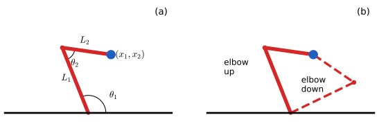
pp. 198–199 Forward problems (causes to effects, joint angles to the position of a robot's hand) usually have one answer; the inverse problems we need to solve (effects to causes, a desired hand position to joint angles) often have several. For the two-link arm of Figure 6.16 every reachable point has two solutions, "elbow up" and "elbow down".
robot_inverse. Reproduces Bishop and Bishop (2024), Figure 6.16. Code: fig_6_16. Download: PDF · SVGFilling the gap 6.12: the arm's kinematics (Exercise 6.16), and why least squares averages the solutions pp. 198–199, 207
Derivation
Forward. Put the base at the origin, let \(\theta_1\) be the angle of the first link from the horizontal and \(\theta_2\) the angle at the elbow between the two links (as drawn in Figure 6.16). The elbow is at \(L_1\mathbf e(\theta_1)\) with \(\mathbf e(\phi)=(\cos\phi,\sin\phi)\). Seen from the elbow, the base lies in direction \(\theta_1+\pi\); rotating that direction by \(\theta_2\) gives the direction of the second link, \(\theta_1+\theta_2+\pi\). Since \(\mathbf e(\phi+\pi)=-\mathbf e(\phi)\),
\[ x_1=L_1\cos\theta_1-L_2\cos(\theta_1+\theta_2),\qquad x_2=L_1\sin\theta_1-L_2\sin(\theta_1+\theta_2). \]Inverse. The hand vector is \(R(\theta_1)\big(L_1-L_2\cos\theta_2,\,-L_2\sin\theta_2\big)^\T\), with \(R\) a rotation, so its length satisfies the law of cosines \(r^2\)
Least squares. For any function \(y(\x)\),
\[ \E\big[\|y(\x)-\tv\|^2\big]=\E\big[\|y(\x)-\E[\tv\given\x]\|^2\big]+\E\big[\|\tv-\E[\tv\given\x]\|^2\big], \]because the cross term has zero conditional mean. The second term does not depend on \(y\), so the best function is the conditional mean \(\E[\tv\given\x]\), and a flexible network trained on the sum of squares approximates it. When \(\tv\given\x\) has two well-separated modes (the two elbows), their average is generally not a solution at all: over the 400 training positions of the robot demo the least-squares arm misses the target by 0.11 (median), the mixture density network's most probable component by 0.025. ∎
See also: Filling the gap 5.8 (why least squares returns the conditional mean) in the companion course.
The book's toy inverse problem is easier to plot: \(x\) uniform on \((0,1)\), \(t=x+0.3\sin(2\pi x)\) plus noise uniform on \((-0.1,0.1)\), and the inverse problem swaps \(x\) and \(t\). A sum-of-squares network fits the forward problem well and the inverse problem badly (Figure 6.17).
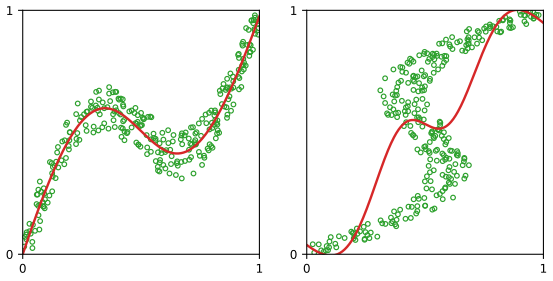
fig_6_17. Download: PDF · SVG6.5.2 Conditional mixture distributions
pp. 199–201
Definition 6.3 (mixture density network) pp. 200–201, (6.38)–(6.43)
For a target \(\tv\in\R^L\), model
\[ p(\tv\given\x)=\sum_{k=1}^{K}\pi_k(\x)\,\N\big(\tv\given\bmu_k(\x),\sigma_k^2(\x)\I\big), \tag{6.38} \]a heteroscedastic model (the spread depends on \(\x\)) that need not factorise over the components of \(\tv\). A network with input \(\x\) has \((L+2)K\) outputs: \(K\) pre-activations \(a^\pi_k\), \(K\) pre-activations \(a^\sigma_k\) and \(KL\) pre-activations \(a^\mu_{kj}\), mapped to valid parameters by
\[ \sum_{k=1}^{K}\pi_k(\x)=1,\qquad 0\le\pi_k(\x)\le1, \tag{6.39} \] \[ \pi_k(\x)=\frac{\exp(a^\pi_k)}{\sum_{l=1}^{K}\exp(a^\pi_l)}, \tag{6.40} \] \[ \sigma_k(\x)=\exp(a^\sigma_k), \tag{6.41} \] \[ \mu_{kj}(\x)=a^\mu_{kj}. \tag{6.42} \]The weights \(\w\) are fitted by minimising the negative log likelihood
\[ E(\w)=-\sum_{n=1}^{N}\ln\Big\{\sum_{k=1}^{K}\pi_k(\x_n,\w)\,\N\big(\tv_n\given\bmu_k(\x_n,\w),\sigma_k^2(\x_n,\w)\I\big)\Big\}. \tag{6.43} \]Unlike a mixture of experts (Jacobs et al. 1991), where each component has its own network, here one network with shared hidden units produces all the parameters. Full covariances can be parametrised through a Cholesky factor (Williams 1996), and other component families (Bernoulli for binary targets) work the same way.
See also: Definition 5.2 and Section 14.5.3, mixtures of experts, in the companion course.
6.5.3 Gradient optimization
pp. 201–202 Automatic differentiation (Chapter 8) would compute the gradient of (6.43), but the derivatives with respect to the output pre-activations have a clear probabilistic meaning. With \(\mathcal N_{nk}\)
the posterior probability of component \(k\) given \(\tv_n\), with \(\pi_k(\x_n)\) as the \(\x\)-dependent prior (Exercise 6.17: Bayes' theorem with \(p(k\given\x)=\pi_k\) and \(p(\tv\given k,\x)=\mathcal N_{nk}\)).
Result 6.8 (error signals of a mixture density network; Exercises 6.17–6.20) p. 202, (6.44)–(6.47)
For the error \(E_n\) of one data point and any target dimension \(L\),
\[ \frac{\partial E_n}{\partial a^\pi_k}=\pi_k-\gamma_{nk}, \tag{6.45} \] \[ \frac{\partial E_n}{\partial a^\mu_{kl}}=\gamma_{nk}\,\frac{\mu_{kl}-t_{nl}}{\sigma_k^2}, \tag{6.46} \] \[ \frac{\partial E_n}{\partial a^\sigma_k}=\gamma_{nk}\Big(L-\frac{\|\tv_n-\bmu_k\|^2}{\sigma_k^2}\Big). \tag{6.47} \]These output error signals are backpropagated through the network like \(y_k-t_k\) in Section 6.4.
Proof
Let \(Z=\sum_l\pi_l\mathcal N_{nl}\), so \(E_n=-\ln Z\) and \(\gamma_{nk}=\pi_k\mathcal N_{nk}/Z\). The log of a component density is \(\ln\mathcal N_{nk}\)
(6.45). \(\partial E_n/\partial\pi_j\)
since the responsibilities sum to 1.
(6.46). Only the \(k\)th term of \(Z\) depends on \(\mu_{kl}=a^\mu_{kl}\): \(\partial E_n/\partial\mu_{kl}\)
(6.47). Similarly \(\partial\ln\mathcal N_{nk}/\partial\sigma_k\)
Interpretation. At a stationary point, summed over the data with fixed hidden features, (6.45) says the predicted \(\pi_k\) match the posterior responsibilities, (6.46) that each mean is a responsibility-weighted average of the targets, and (6.47) that \(\sigma_k^2\) matches the responsibility-weighted squared error per dimension: the M-step of EM for a Gaussian mixture, made input-dependent. Numerical tests compare all three with automatic differentiation for \(L=2\), \(K=3\) (agreement to \(10^{-15}\)), and the backpropagated network gradient with finite differences. ∎
See also: Result 5.18 (the same derivatives in Bishop 2006) in the companion course.
6.5.4 Predictive distribution
pp. 202–204 A trained mixture density network gives the whole conditional density for any \(\x\). Although its outputs are continuous single-valued functions of \(\x\), the density can be unimodal for some inputs and trimodal for others because the mixing coefficients switch components on and off (Figure 6.19). Summaries follow from (6.38):
\[ \E[\tv\given\x]=\int\tv\,p(\tv\given\x)\,\d\tv=\sum_{k=1}^{K}\pi_k(\x)\bmu_k(\x), \tag{6.48} \]the quantity a least-squares network approximates, and the conditional variance about it,
\[ s^2(\x)=\E\big[\|\tv-\E[\tv\given\x]\|^2\given\x\big]. \tag{6.49} \]Result 6.9 (conditional mean and variance; Exercise 6.21) p. 203, (6.48)–(6.50)
For the mixture (6.38) with \(\tv\in\R^L\), the mean is (6.48) and
\[ s^2(\x)=\sum_{k=1}^{K}\pi_k(\x)\Big\{L\,\sigma_k^2(\x)+\Big\|\bmu_k(\x)-\sum_{l=1}^{K}\pi_l(\x)\bmu_l(\x)\Big\|^2\Big\}. \tag{6.50, corrected} \]Erratum. The book's (6.50) and the official solution of Exercise 6.21 have \(\sigma_k^2\) in place of \(L\sigma_k^2\), which is right only for a scalar target. For \(L=2\) and \(K=3\), 400 000 samples from a mixture give \(s^2=49.31\); the corrected formula gives 49.30 and the printed one 25.23.
Proof
Write \(\bar\tv=\sum_l\pi_l\bmu_l\). The mean: \(\int\tv\sum_k\pi_k\mathcal N_k\,\d\tv\)
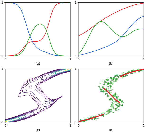
fig_6_19. Download: PDF · SVGFor a multimodal density the mean (6.48) can be useless: the average of the two arm configurations is not a configuration. The conditional mode is better, but has no closed form. The book's shortcut takes the mean of the component with the largest \(\pi_k\) (Figure 6.19(d)); an exact mode is easy to compute.
Filling the gap 6.13: computing the conditional mode pp. 203–204
Derivation
Fix \(\x\) and write \(p(\tv)=\sum_k\pi_k\mathcal N_k(\tv)\) with \(\mathcal N_k\)
It never decreases \(p\). For the current \(\tv_0\), Jensen's inequality gives, for every \(\tv\), \(\ln p(\tv)\)mdn_mode). ∎
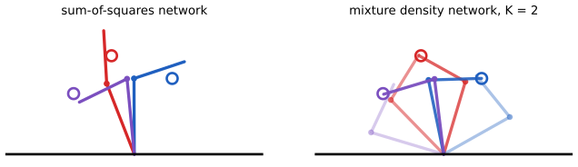
fig_robot_mdn. Download: PDF · SVGSee also: the mixture density demo (the one-dimensional toy problem of Figures 6.17 and 6.19) and Result 5.19 in the companion course.
Exercises
All 21 exercises of Chapter 6 (pp. 204–207), restated in my own words, with complete solutions (hidden). Stars give the book's difficulty. Each was solved independently and then compared with the official solutions manual (version 1.0); where the manual is wrong this is said, with the evidence.
Exercise 6.1 (★★★). Using \(\int_{-\infty}^\infty e^{-x^2}\d x\)
\({}=\sqrt\pi\) and the polar-coordinate identity (6.51), with the gamma function (6.52), show that the unit sphere in \(\R^D\) has area \(S_D=2\pi^{D/2}/\Gamma(D/2)\) (6.53) and the unit ball volume \(V_D=S_D/D\) (6.54); check \(D=2,3\) with \(\Gamma(1)=1\), \(\Gamma(3/2)=\sqrt\pi/2\). Solution
The left side of (6.51) is \((\sqrt\pi)^D=\pi^{D/2}\); the right side, with \(u=r^2\), is \(\tfrac12S_D\Gamma(D/2)\). So \(S_D=2\pi^{D/2}/\Gamma(D/2)\). Integrating the shells, \(V_D=\int_0^1S_Dr^{D-1}\d r=S_D/D\). \(D=2\): \(S_2=2\pi\), \(V_2=\pi\). \(D=3\): \(S_3=2\pi^{3/2}/(\sqrt\pi/2)=4\pi\), \(V_3=4\pi/3\). Details: Result 6.1. (The manual writes \(V_2=\pi a^2\), \(V_3=\tfrac43\pi a^3\), i.e. for radius \(a\) rather than 1.)
Exercise 6.2 (★★★). Show that a ball of radius \(a\) fills the fraction (6.55) of the cube of side \(2a\) around it, that this tends to 0 as \(D\to\infty\) (use Stirling's formula \(\Gamma(x+1)\)
\({}\simeq\sqrt{2\pi}e^{-x}x^{x+1/2}\), (6.56)), and that the distance from the centre to a corner divided by the distance to a face is \(\sqrt D\). Solution
Ratio \(V_Da^D/(2a)^D\)
\({}=\pi^{D/2}/(D2^{D-1}\Gamma(D/2))\). Applying (6.56) with \(x=D/2-1\), or equivalently \(\Gamma(D/2)\sim\sqrt{4\pi/D}(D/2e)^{D/2}\), the ratio behaves like \((\pi e/2D)^{D/2}/\sqrt{\pi D}\to0\) (super-exponentially). Corner \(a\sqrt D\), face \(a\), ratio \(\sqrt D\). See Result 6.1. Note on the manual: it gives the asymptotic form \((\pi e/2D)^{D/2}/D\); the conclusion is right, but the polynomial prefactor is \(1/\sqrt{\pi D}\) (at \(D=800\) the manual's form is off by a factor of 16, the corrected one by 0.02%). Exercise 6.3 (★★★). For \(\x\sim\N(\mathbf 0,\sigma^2\I_D)\) (6.57), show that the radial density is (6.58), that it has a single maximum near \(\hat r\simeq\sqrt D\sigma\), that \(p(\hat r+\epsilon)\) decays away from it on the scale \(\sigma\), and that the density at the origin is \(e^{D/2}\) times that at radius \(\hat r\).
Solution
All in Result 6.1(3): the shell has volume \(S_Dr^{D-1}\epsilon\); \(\hat r=\sqrt{D-1}\sigma\); \((\ln p)''(\hat r)=-2/\sigma^2\), so \(p(\hat r+\epsilon)\)
\({}\simeq p(\hat r)e^{-\epsilon^2/\sigma^2}\); the density ratio is \(e^{(D-1)/2}\simeq e^{D/2}\). The exercise's (6.59), \(p(\hat r)\exp(-3\epsilon^2/2\sigma^2)\), is incorrect, and so is the manual's claim that the expansion yields it. With \((D-1)\ln(1+\epsilon/\hat r)\) \({}=(D-1)(\epsilon/\hat r-\epsilon^2/2\hat r^2+\dots)\) and \(\hat r^2=(D-1)\sigma^2\), the quadratic terms are \(-\epsilon^2/2\sigma^2\) (from the logarithm) and \(-\epsilon^2/2\sigma^2\) (from \(-(\hat r+\epsilon)^2/2\sigma^2\)), total \(-\epsilon^2/\sigma^2\). The manual also writes the density at the origin as \((2\pi\sigma^2)^{-1/2}\); it is \((2\pi\sigma^2)^{-D/2}\) (the ratio is unaffected). Exercise 6.4 (★★). Show that a two-layer network (6.11) with logistic-sigmoid hidden units is equivalent to one with tanh hidden units whose parameters are linear transformations of the original ones.
Solution
\(\sigma(a)=\tfrac12(1+\tanh(a/2))\), so halve all first-layer weights and biases, halve the output weights \(w^{(2)}_{kj}\) (\(j\ge1\)), and set the output bias to \(w^{(2)}_{k0}+\tfrac12\sum_{j\ge1}w^{(2)}_{kj}\): Result 6.3(2). Manual: its bias formula \(\tilde w^{(2)}_{k0}\)
\({}=\tfrac12w^{(2)}_{k0}+\tfrac12\) is wrong (the \(\tfrac12\) must multiply the sum of the output weights, and the original bias is kept); numerically it changes the outputs by order 1. Exercise 6.5 (★★). Plot swish \(x\sigma(\beta x)\) (6.61) and its derivative for \(\beta=0.1,1,10\), and show that it tends to the ReLU as \(\beta\to\infty\).
Solution
See the swish figure. Pointwise: for \(x>0\), \(\sigma(\beta x)\to1\); for \(x<0\), \(\sigma(\beta x)\to0\); at 0 the value is 0. In fact the convergence is uniform with \(\sup|x\sigma(\beta x)-\relu(x)|\)
\({}=W(1/e)/\beta\) (Filling the gap 6.7); as \(\beta\to0\) swish tends to \(x/2\). Exercise 6.6 (★). Express the derivative of tanh in terms of tanh itself.
Solution
Quotient rule on (6.14): \(\tanh'\)
\({}=\frac{(e^a+e^{-a})^2-(e^a-e^{-a})^2}{(e^a+e^{-a})^2}\) \({}=1-\tanh^2a\). Equivalently from \(\tanh a=2\sigma(2a)-1\) (Result 6.3). Exercise 6.7 (★★). Prove the softplus identities (6.62)–(6.65).
Solution
Result 6.3(3): \(\zeta(a)-\zeta(-a)\)
\({}=\ln\frac{1+e^a}{1+e^{-a}}\) \({}=a\); \(\ln\sigma(a)=-\ln(1+e^{-a})=-\zeta(-a)\); \(\zeta'=\sigma\); \(\zeta^{-1}(a)=\ln(e^a-1)\) for \(a>0\). Exercise 6.8 (★). Show that minimising (6.25) over \(\sigma^2\) gives (6.27).
Solution
\(\partial/\partial\sigma^2\) of (6.25) is \(-S/(2\sigma^4)+N/(2\sigma^2)\) with \(S\) the sum of squared residuals; it vanishes at \(\sigma^2=S/N\), a minimum (Filling the gap 6.10).
Exercise 6.9 (★). Show that maximum likelihood under (6.28) is minimisation of (6.29), and that the noise variance is (6.30).
Solution
\(-\ln\prod_n\N(\tv_n\given\y_n,\sigma^2\I)\)
\({}=\frac{1}{2\sigma^2}\sum_n\|\y_n-\tv_n\|^2+\frac{NK}2\ln(2\pi\sigma^2)\); the \(\w\)-part is (6.29) times \(1/\sigma^2\), and the \(\sigma^2\)-derivative vanishes at (6.30) (Filling the gap 6.10). Exercise 6.10 (★★). With Gaussian noise of covariance \(\bm\Sigma\) on vector targets (6.66), give the error for known \(\bm\Sigma\), and the maximum likelihood \(\bm\Sigma\) when it is unknown; note the coupling.
Solution
Known: \(E(\w)\)
\({}=\tfrac12\sum_n(\tv_n-\y_n)^\T\bm\Sigma^{-1}(\tv_n-\y_n)\). Unknown: \(\bm\Sigma_{\rm ML}\) \({}=\frac1N\sum_n(\tv_n-\y_n)(\tv_n-\y_n)^\T\), which depends on \(\w\); the profile error is \(\tfrac N2\ln|\bm\Sigma_{\rm ML}(\w)|\) (Filling the gap 6.10). Agrees with the manual. Exercise 6.11 (★★). Labels are flipped with probability \(\epsilon\). Write the negative log likelihood and check that \(\epsilon=0\) gives (6.33).
Solution
\(E\)
\({}=-\sum_n\{t_n\ln\tilde y_n+(1-t_n)\ln(1-\tilde y_n)\}\) with \(\tilde y_n\) \({}=(1-\epsilon)y_n+\epsilon(1-y_n)\); \(\epsilon=0\) gives (6.33). Each term is bounded by \(\ln(1/\epsilon)\), hence robustness (Filling the gap 6.11). Exercise 6.12 (★★). Derive the error for targets \(t\in\{-1,1\}\) and outputs in \([-1,1]\), and the matching output activation.
Solution
Output \(y=\tanh(a/2)\)
\[ E=-\tfrac12\sum_n\{(1+t_n)\ln(1+y_n)+(1-t_n)\ln(1-y_n)\} \]\({}=2\sigma(a)-1\), error (plus the constant \(N\ln2\)); \(\partial E_n/\partial a_n=(y_n-t_n)/2\) (Filling the gap 6.11). Agrees with the manual.
Exercise 6.13 (★). Show that maximum likelihood for a multiclass network with \(y_k=p(t_k=1\given\x)\) is minimisation of (6.36).
Solution
With 1-of-\(K\) targets \(p(\tv\given\x)=\prod_ky_k^{t_k}\); the negative log of \(\prod_n\prod_ky_{nk}^{t_{nk}}\) is (6.36) (Result 6.7).
Exercise 6.14 (★). Show that for a logistic-sigmoid output the derivative of (6.33) with respect to the pre-activation is \(y-t\).
Solution
\(\partial E_n/\partial y_n\)
\({}=-t_n/y_n+(1-t_n)/(1-y_n)\) and \(\partial y_n/\partial a_n=y_n(1-y_n)\); the product is \(-t_n(1-y_n)+(1-t_n)y_n=y_n-t_n\). Exercise 6.15 (★). Show that for softmax outputs (6.37) the derivative of (6.36) with respect to \(a_k\) is \(y_k-t_k\).
Solution
\(\partial y_j/\partial a_k\)
\({}=y_j(\delta_{jk}-y_k)\) and \(\partial E_n/\partial y_j=-t_j/y_j\), so \(\partial E_n/\partial a_k\) \({}=-\sum_jt_j(\delta_{jk}-y_k)\) \({}=y_k-t_k\) using \(\sum_jt_j=1\) (Result 6.7). Exercise 6.16 (★★). Write the forward kinematics of the arm of Figure 6.16: \((x_1,x_2)\) in terms of \(\theta_1,\theta_2,L_1,L_2\), with the origin at the base.
Solution
\(x_1\)
\({}=L_1\cos\theta_1-L_2\cos(\theta_1+\theta_2)\), \(x_2\) \({}=L_1\sin\theta_1-L_2\sin(\theta_1+\theta_2)\), with \(\theta_2\) the angle between the links at the elbow; the inverse has the two solutions of Filling the gap 6.12. Agrees with the manual, whose intermediate line has a typo (\(L_1\) for \(L_2\) in the second coordinate). Exercise 6.17 (★★). Show that \(\gamma_{nk}\) (6.44) is the posterior probability of component \(k\) given \(\tv_n\), with \(\pi_k(\x)\) as prior.
Solution
Introduce the latent component \(k\) with \(p(k\given\x)=\pi_k(\x)\) (valid by (6.39)) and \(p(\tv\given k,\x)\)
\({}=\N(\tv\given\bmu_k,\sigma_k^2\I)\); then (6.38) is \(\sum_kp(k\given\x)p(\tv\given k,\x)\), and Bayes' theorem gives \(p(k\given\tv_n,\x_n)\) \({}=\pi_k\mathcal N_{nk}/\sum_l\pi_l\mathcal N_{nl}\) \({}=\gamma_{nk}\). Numerical tests also confirm it by sampling: among mixture samples near a given \(\tv\), the component frequencies match \(\gamma_k\). Exercise 6.18 (★★). Derive (6.45).
Solution
Chain rule through all \(\pi_j\): \(-\sum_j(\gamma_{nj}/\pi_j)\pi_j(\delta_{jk}-\pi_k)\)
\({}=\pi_k-\gamma_{nk}\) (Result 6.8). Exercise 6.19 (★★). Derive (6.46).
Solution
\(\partial E_n/\partial\mu_{kl}\)
\({}=-\gamma_{nk}\,\partial\ln\mathcal N_{nk}/\partial\mu_{kl}\) \({}=\gamma_{nk}(\mu_{kl}-t_{nl})/\sigma_k^2\), and \(a^\mu_{kl}=\mu_{kl}\) (Result 6.8). Exercise 6.20 (★★). Derive (6.47).
Solution
\(\partial\ln\mathcal N_{nk}/\partial\sigma_k\)
\({}=-L/\sigma_k+\|\tv_n-\bmu_k\|^2/\sigma_k^3\) and \(\partial\sigma_k/\partial a^\sigma_k\) \({}=\sigma_k\), so \(\partial E_n/\partial a^\sigma_k\) \({}=\gamma_{nk}(L-\|\tv_n-\bmu_k\|^2/\sigma_k^2)\) (Result 6.8). The manual's final answer agrees; its intermediate expression for \(\partial E_n/\partial\sigma_k\) drops the mixing coefficients and writes \((L/2\pi)^{L/2}\) for the normalising constant \((2\pi)^{-L/2}\), slips that cancel in the final line. Exercise 6.21 (★★★). Verify the conditional mean (6.48) and variance (6.50).
Solution
See Result 6.9. The mean is linearity of the integral. The variance is \(\sum_k\pi_k\{L\sigma_k^2+\|\bmu_k-\bar\tv\|^2\}\): for \(L\)-dimensional isotropic components the within-component term is \(L\sigma_k^2\), not \(\sigma_k^2\) as printed in (6.50) and used in the manual (which takes \(\int\tv^\T\tv\,\N(\tv\given\bmu_k,\sigma_k^2\I)\d\tv\)
\({}=\sigma_k^2+\bmu_k^\T\bmu_k\)). The two agree for \(L=1\), the case of Figure 6.19.
Demonstrations for this chapter
Each demonstration runs in the browser with seeded random numbers, so a class sees the same pictures, and links back to these notes. The ▶ Demo boxes above open them set to the case under discussion. For each, the Python code reproduces the page's numbers for the same settings.
| Demonstration | What you can see | Sections and results |
|---|---|---|
| The curse of dimensionality | Shell volume, the Gaussian radius, concentration of distances and empty grid cells, Monte Carlo against the formulas, and the grid classifier on the Iris data. Presets: 1 \(D=2\); 2 \(D=20\) (Figs. 6.4, 6.5); 3 \(D=200\); 4 Iris grid classifier (Fig. 6.2); 5 empty cells (Fig. 6.3). | 6.1.1, 6.1.2; Result 6.1, gaps 6.2, 6.3 |
| Universal approximation and activation functions | A two-layer network trained live (Adam, backpropagation) with eight activation functions; hidden-unit contributions, \(h\) and \(h'\), saturated and dead units. Presets: 1 \(x^2\) (Fig. 6.10a); 2 step (Fig. 6.10d); 3 \(|x|\) with two ReLUs; 4 ReLU sine, dead units; 5 saturated tanh. | 6.2.2, 6.2.3; Results 6.2, 6.3, gap 6.6 |
| Linear regions of ReLU networks | Regions of random networks on the square, exact and grid counts, the one-layer and Montúfar bounds, and the sawtooth. Presets: 1 \(1\times24\); 2 \(3\times8\); 3 \(6\times4\); 4 sawtooth \(L=4\); 5 sawtooth \(L=8\). | 6.3; Results 6.5, 6.6 |
| Robot-arm inverse kinematics with a mixture density network | Least squares against MDNs with \(K=1,2,3\) trained live, a draggable target, the conditional density over joint angles, and a gradient check of (6.45)–(6.47). Presets: 1 least squares; 2 \(K=2\); 3 \(K=1\); 4 gradient check; 5 \(K=3\). | 6.5; Result 6.8, gap 6.12 |
The Python code that produces every figure of this page is code/ch06_deep_neural_networks.py (see the code index).
References
- Bishop, C. M. and Bishop, H. (2024). Deep Learning: Foundations and Concepts. Springer, Cham. Chapter 6, pp. 171–207; and the official solutions manual, version 1.0. www.bishopbook.com.
- Barron, A. R. (1993). Universal approximation bounds for superpositions of a sigmoidal function. IEEE Transactions on Information Theory, 39(3), 930–945.
- Bellman, R. (1961). Adaptive Control Processes: A Guided Tour. Princeton University Press.
- Bengio, Y., Courville, A. and Vincent, P. (2013). Representation learning: a review and new perspectives. IEEE Transactions on Pattern Analysis and Machine Intelligence, 35(8), 1798–1828.
- Beyer, K., Goldstein, J., Ramakrishnan, R. and Shaft, U. (1999). When is "nearest neighbor" meaningful? In Database Theory, ICDT'99, Lecture Notes in Computer Science 1540, 217–235. Springer.
- Bishop, C. M. (1994). Mixture density networks. Technical Report NCRG/94/004, Aston University.
- Bishop, C. M. (2006). Pattern Recognition and Machine Learning. Springer, New York.
- Broomhead, D. S. and Lowe, D. (1988). Multivariable functional interpolation and adaptive networks. Complex Systems, 2, 321–355.
- Carreira-Perpiñán, M. Á. (2000). Mode-finding for mixtures of Gaussian distributions. IEEE Transactions on Pattern Analysis and Machine Intelligence, 22(11), 1318–1323.
- Caruana, R. (1997). Multitask learning. Machine Learning, 28, 41–75.
- Chen, A. M., Lu, H. and Hecht-Nielsen, R. (1993). On the geometry of feedforward neural network error surfaces. Neural Computation, 5(6), 910–927. doi:10.1162/neco.1993.5.6.910.
- Chen, T., Kornblith, S., Norouzi, M. and Hinton, G. (2020). A simple framework for contrastive learning of visual representations. In Proceedings of the 37th International Conference on Machine Learning, PMLR 119, 1597–1607.
- Collobert, R. (2004). Large Scale Machine Learning. PhD thesis, Université Paris VI.
- Cybenko, G. (1989). Approximation by superpositions of a sigmoidal function. Mathematics of Control, Signals and Systems, 2(4), 303–314. doi:10.1007/BF02551274.
- Fisher, R. A. (1936). The use of multiple measurements in taxonomic problems. Annals of Eugenics, 7(2), 179–188.
- Funahashi, K. (1989). On the approximate realization of continuous mappings by neural networks. Neural Networks, 2(3), 183–192. doi:10.1016/0893-6080(89)90003-8.
- Gutmann, M. and Hyvärinen, A. (2010). Noise-contrastive estimation: a new estimation principle for unnormalized statistical models. In Proceedings of the 13th International Conference on Artificial Intelligence and Statistics, PMLR 9, 297–304.
- Hanin, B. and Rolnick, D. (2019). Complexity of linear regions in deep networks. In Proceedings of the 36th International Conference on Machine Learning, PMLR 97, 2596–2604.
- Hornik, K. (1991). Approximation capabilities of multilayer feedforward networks. Neural Networks, 4(2), 251–257. doi:10.1016/0893-6080(91)90009-T.
- Hornik, K., Stinchcombe, M. and White, H. (1989). Multilayer feedforward networks are universal approximators. Neural Networks, 2(5), 359–366. doi:10.1016/0893-6080(89)90020-8.
- Hospedales, T., Antoniou, A., Micaelli, P. and Storkey, A. (2021). Meta-learning in neural networks: a survey. IEEE Transactions on Pattern Analysis and Machine Intelligence, 44(9), 5149–5169.
- Jacobs, R. A., Jordan, M. I., Nowlan, S. J. and Hinton, G. E. (1991). Adaptive mixtures of local experts. Neural Computation, 3(1), 79–87.
- Khosla, P., Teterwak, P., Wang, C., Sarna, A., Tian, Y., Isola, P., Maschinot, A., Liu, C. and Krishnan, D. (2020). Supervised contrastive learning. In Advances in Neural Information Processing Systems 33.
- Krizhevsky, A., Sutskever, I. and Hinton, G. E. (2012). ImageNet classification with deep convolutional neural networks. In Advances in Neural Information Processing Systems 25, 1097–1105.
- Kůrková, V. and Kainen, P. C. (1994). Functionally equivalent feedforward neural networks. Neural Computation, 6(3), 543–558. doi:10.1162/neco.1994.6.3.543.
- LeCun, Y., Bottou, L., Bengio, Y. and Haffner, P. (1998). Gradient-based learning applied to document recognition. Proceedings of the IEEE, 86(11), 2278–2324. doi:10.1109/5.726791.
- Leshno, M., Lin, V. Ya., Pinkus, A. and Schocken, S. (1993). Multilayer feedforward networks with a nonpolynomial activation function can approximate any function. Neural Networks, 6(6), 861–867. (The book's bibliography drops the "non" from the title.)
- Montúfar, G., Pascanu, R., Cho, K. and Bengio, Y. (2014). On the number of linear regions of deep neural networks. In Advances in Neural Information Processing Systems 27, 2924–2932.
- Oord, A. van den, Li, Y. and Vinyals, O. (2018). Representation learning with contrastive predictive coding. arXiv:1807.03748.
- Opper, M. and Winther, O. (2000). Gaussian processes and SVM: mean field theory and leave-one-out. In A. J. Smola, P. L. Bartlett, B. Schölkopf and D. Schuurmans (eds), Advances in Large Margin Classifiers, 311–326. MIT Press.
- Radford, A., Kim, J. W., Hallacy, C. et al. (2021). Learning transferable visual models from natural language supervision. In Proceedings of the 38th International Conference on Machine Learning, PMLR 139, 8748–8763.
- Ramachandran, P., Zoph, B. and Le, Q. V. (2017). Searching for activation functions. arXiv:1710.05941.
- Simard, P. Y., Steinkraus, D. and Platt, J. C. (2003). Best practices for convolutional neural networks applied to visual document analysis. In Seventh International Conference on Document Analysis and Recognition, 958–963. doi:10.1109/ICDAR.2003.1227801.
- Sussmann, H. J. (1992). Uniqueness of the weights for minimal feedforward nets with a given input-output map. Neural Networks, 5(4), 589–593.
- Telgarsky, M. (2016). Benefits of depth in neural networks. In 29th Annual Conference on Learning Theory, PMLR 49, 1517–1539.
- Vapnik, V. N. (1995). The Nature of Statistical Learning Theory. Springer, New York.
- Williams, P. M. (1996). Using neural networks to model conditional multivariate densities. Neural Computation, 8(4), 843–854.
The numerical statements in the text (coefficient counts, sphere and cube volumes and their asymptotics, the Gaussian shell and the corrected (6.59), concentration, the empty-cell formula, the sigmoid–tanh weight map, activation derivatives against automatic differentiation, the swish constant, the symmetry orbit, the universal-approximation constructions, the arrangement and sawtooth counts, InfoNCE and CLIP, the error-function identities, the MDN gradients, moments, posterior and mode, the robot-arm kinematics, and the agreement of the four demonstrations with the Python code) were confirmed numerically.