Transformers
A transformer maps a set of \(N\) token vectors to another set of \(N\) vectors of the same size, and the core of the map is attention: each output is a weighted average of value vectors, with weights computed from the data themselves. This chapter builds the transformer layer step by step (Section 12.1: attention, scaling, multiple heads, residual connections and normalisation, cost, positional encoding), turns text into tokens and reviews the language models that came before (12.2: embeddings, byte-pair encoding, bag of words, n-grams, recurrent networks), uses transformers as language models (12.3: decoders and the causal mask, sampling strategies, encoders, sequence-to-sequence models, large language models and fine-tuning), and applies the same layer to images, audio and mixtures of modalities (12.4).
Ch. 1 Deep learning revolution Ch. 2 Probabilities Ch. 3 Standard distributions Ch. 4 Regression Ch. 5 Classification Ch. 6 Deep neural networks Ch. 7 Gradient descent Ch. 8 Backpropagation Ch. 9 Regularization Ch. 10 Convolutional networks Ch. 11 Structured distributions Ch. 12 Transformers Ch. 13 Graph neural networks Ch. 14 Sampling Ch. 15 Discrete latent variables Ch. 16 Continuous latent variables Ch. 17 GANs Ch. 18 Normalizing flows Ch. 19 Autoencoders Ch. 20 Diffusion models Appendices A to C
How to read these notes
They follow the book. Sections carry the book's numbers (12.1, 12.3.2, ...) and every displayed equation that appears in the book carries the book's own equation number, e.g. (12.14), so the notes can be read next to the book. Equations without a number are steps that the book skips.
Filling the gaps. Wherever the book states a result without proof, says it "can be shown", or leaves it to an exercise, an orange Filling the gap box or a proof gives the full argument. Proofs and derivations start hidden: open one with its bar, or use the button below.
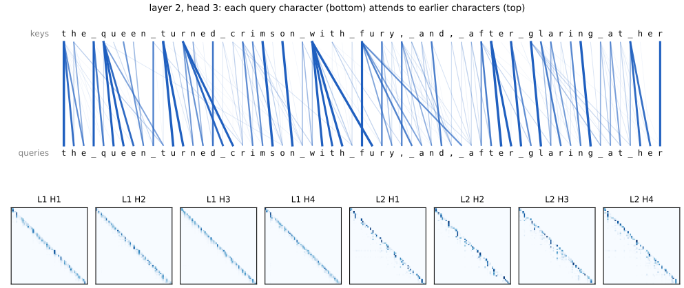
Figures and demonstrations. The chapter's figures are mostly architecture diagrams; the seven that show computed or measured results are reproduced by the Python code, three of them (12.2, 12.17, 12.24) by small models trained here on one CPU core, as the book's versions come from large published models. Eight supplementary figures (12.S1 to 12.S8, our own) illustrate the gaps that are filled. The ▶ Demo boxes open an interactive demonstration already set to the case being discussed.
Main reference
C. M. Bishop and H. Bishop, Deep Learning: Foundations and Concepts, Springer (2024), Chapter 12, pages 357–406. Section, equation, figure and exercise numbers below refer to this book. Further reading is listed in the references; the book's website is www.bishopbook.com. There is no official solutions manual for this chapter: all solutions below are my own.
The explanations, derivations, figures and code are my own; equations are cited by their numbers in the book.
Companion course: Bayesian and Probabilistic Machine Learning
Transformers are new relative to the companion course Bayesian and Probabilistic Machine Learning (Bishop 2006), but many of the tools used here are proved in full there. These notes state such results with a short argument and link the full treatment.
- The softmax and its derivatives, multiclass logistic regression: Section 4.3.4 (here 12.1.3, 12.1.5, 12.3.3).
- Kernel regression, the Nadaraya–Watson model, of which soft attention is a learned version: Section 6.3.1 (here Filling the gap 12.1).
- Error backpropagation: Section 5.3 (here Result 12.3 and 12.2.6); convolutional networks and weight sharing: Section 5.5.6 (here 12.4.1).
- Geometry of high-dimensional spaces: Section 1.4 (here Exercise 12.8); entropy, cross-entropy and relative entropy: Section 1.6 (here perplexity in 12.2.4 and the sampling rules in 12.3.2).
- Maximum likelihood for multinomial variables and Dirichlet smoothing: Section 2.2, 2.2.1; Lagrange multipliers: toolkit; naive Bayes with discrete features: Section 4.2.3 (here 12.2.3, Exercises 12.1, 12.11).
- Factorising a joint distribution along a graph: Section 8.1; Markov chains (n-gram models), hidden Markov models and the Viterbi algorithm: Section 13.1, 13.2, 13.2.5 (here 12.2.4, 12.3.2).
- K-means clustering and vector quantisation: Section 9.1, 9.1.1 (here 12.4.2); low-rank approximation: Section 12.1.2 (here LoRA, 12.3.5).
- Autoregressive generative models: the lecture on autoregressive models in the advanced module, with its pixel-by-pixel generation demo (here 12.3.1 and 12.4.2).
The chapter at a glance
- 12.1 Attention outputs \(\by_n=\sum_ma_{nm}\bv_m\) with weights \(a_{nm}=\Softmax\) of query-key scores (Definition 12.1): a learned kernel smoother (Filling the gap 12.1). The claim that orthogonal inputs pass through unchanged is false (Result 12.1). The softmax Jacobian vanishes as the softmax saturates (Result 12.2); the backward pass of attention is written out (Result 12.3); dividing the scores by \(\sqrt{D}\) keeps their variance at 1 for every \(D\) (Result 12.4). Multi-head attention is a sum of low-rank heads (Result 12.5, a corrected Exercise 12.5); parameter and operation counts, BERT included (Results 12.6, 12.7). Without positions a transformer is permutation equivariant (Result 12.8); sinusoidal encodings turn a shift of position into a rotation, so relative positions are linear (Result 12.9).
- 12.2 Skip-gram embeddings factorise a shifted pointwise mutual information matrix (Result 12.10); byte-pair encoding (Algorithm 12.4, Figure 12.12); maximum likelihood for bag-of-words and n-gram tables (Result 12.11); cross-entropy and perplexity (Definition 12.2): a 105 000-parameter transformer beats every n-gram model on held-out text (Figure 12.S4). Gradients through time are products of Jacobians (Filling the gap 12.7).
- 12.3 The causal mask makes output \(n\) depend only on tokens \(1..n\), so one pass trains all \(N\) next-token predictions at once (Result 12.12). Temperature, top-k and nucleus sampling (Result 12.13); greedy and beam search are heuristics, and beam search can do worse than greedy (Result 12.14; Exercise 12.15 as printed has an inconsistent table). Encoders, cross-attention (Result 12.15) and low-rank adaptation (Result 12.16).
- 12.4 Patch embeddings are strided convolutions (Filling the gap 12.9); a 105 000-parameter vision transformer reaches 93.7% on MNIST (Figure 12.S7); why image tokens are discrete (Filling the gap 12.10) and how vector quantisation makes them; mel spectrograms (Definition 12.3).
Notation. \(\bX\in\R^{N\times D}\) is the data matrix whose \(n\)th row is the token \(\bx_n^\T\) (Figure 12.3). Queries, keys and values are \(\bQ=\bX\bW^{(q)}\), \(\bK=\bX\bW^{(k)}\), \(\bV=\bX\bW^{(v)}\), with rows \(\bq_n^\T\), \(\bkk_m^\T\), \(\bv_m^\T\) of lengths \(D_k\), \(D_k\), \(D_v\). \(\bA=(a_{nm})\) is the \(N\times N\) matrix of attention weights, \(\Softmax[\cdot]\) acts on each row of a matrix, \(H\) is the number of heads, \(D_{\rm ff}\) the hidden width of the MLP, \(K\) the vocabulary size, \(T\) the temperature (\(^\T\) is the transpose), and \(\bP\) a permutation matrix.
Printings. The first printing has a few slips in this chapter: a false claim about orthogonal inputs (p. 363 and Exercise 12.3), a dimension error in Exercise 12.5, an inconsistent table in Exercise 12.15, and typographical errors in Algorithms 12.1 and 12.2. Each is flagged with an Erratum note where it occurs, and the list with the evidence is in the corrections.
pp. 357–358 A transformer takes a set of vectors and returns a set of vectors of the same number and dimension, in a representation meant to be more useful for whatever comes next. Three properties explain its dominance, and the chapter returns to each: it transfers well (a model pre-trained on a large unlabelled corpus is fine-tuned for many tasks, a foundation model; see Section 6.3.4 on transfer learning); it can be trained by self-supervision, because a text supplies its own targets; and its computations are large matrix products that parallel hardware executes efficiently, so that models of up to about \(10^{12}\) parameters can be trained. The book also mentions the scaling hypothesis: performance keeps improving as the number of parameters and the data grow together, with no change of architecture (see Section 1.1.4).
12.1 Attention
pp. 358–360 Attention was introduced to improve recurrent translation models (Bahdanau, Cho and Bengio, 2014); Vaswani et al. (2017) showed that it works better on its own, without the recurrence. The motivating observation is that the meaning of a word depends on its context, and on some words of the context much more than on others: in "I swam across the river to get to the other bank", the words "swam" and "river" decide which "bank" is meant (Figure 12.1). A fixed network weights its inputs by fixed numbers; attention weights them by numbers computed from the inputs, so that which words matter can change from sentence to sentence. A transformer can thus be seen as a context-dependent embedding: the same word is mapped to different places for different contexts.
12.1.1 Transformer processing
pp. 360–361 The input is a set of \(N\) tokens \(\bx_1,\dots,\bx_N\in\R^D\), whose components are features; a token may be a word or part of a word, an image patch, an amino acid. The tokens are stacked as the rows of \(\bX\in\R^{N\times D}\) (Figure 12.3), and a transformer layer is a map
\[ \widetilde\bX=\operatorname{TransformerLayer}[\bX] \tag{12.1} \]with \(\widetilde\bX\in\R^{N\times D}\) again. A layer has two stages: attention, which mixes information across tokens (it combines rows), and a position-wise network, which transforms the features within each token (it acts on each row separately with shared weights). Layers are stacked, each with its own parameters. Because the same weights are used for every row, the same layer accepts any \(N\).
12.1.2 Attention coefficients
Definition 12.1 (attention weights) pp. 361–362, (12.2)–(12.4)
An attention layer produces each output as a combination of the inputs,
\[ \by_n=\sum_{m=1}^Na_{nm}\bx_m, \tag{12.2} \]with weights that are non-negative and sum to one over \(m\), separately for each \(n\):
\[ a_{nm}\ge0, \tag{12.3} \] \[ \sum_{m=1}^Na_{nm}=1. \tag{12.4} \]So each row of \(\bA=(a_{nm})\) is a probability vector (a partition of unity), \(\by_n\) is a convex combination of the inputs and lies in their convex hull, and in particular \(0\le a_{nm}\le1\) (Exercise 12.1). In matrix form \(\bY=\bA\bX\), with \(\bA\) a row-stochastic matrix that depends on \(\bX\).
The non-negativity rules out the degenerate situation of two large weights of opposite sign cancelling, and the sum-to-one constraint makes attention a budget: more attention to one input means less to the others. If \(a_{mm}=1\) then all other weights in row \(m\) vanish and \(\by_m=\bx_m\).
12.1.3 Self-attention
See also the companion course, Section 4.3.4 (the softmax) and Section 6.3.1 (Nadaraya–Watson kernel regression); and Section 5.4.4 of this course.
pp. 362–363 The weights come from an analogy with information retrieval. Each item in a catalogue has a key (a description) and a value (the item itself); a user sends a query; the service compares the query with every key and returns the value of the best match. That is hard attention. A transformer uses soft attention: it returns an average of all values, weighted by how well each key matches the query, which is differentiable and so can be trained by gradient descent. In the simplest version the token itself serves as query, key and value, similarity is the dot product, and the softmax turns similarities into weights satisfying (12.3) and (12.4):
\[ a_{nm}=\frac{\exp(\bx_n^\T\bx_m)}{\sum_{m'=1}^N\exp(\bx_n^\T\bx_{m'})}, \tag{12.5} \] \[ \bY=\Softmax\big[\bX\bX^\T\big]\bX, \tag{12.6} \]where \(\Softmax[\bL]\) exponentiates every element of \(\bL\) and normalises each row to sum to one. As the book stresses, the softmax here is a normalisation device, not a probability model. Because queries, keys and values come from the same sequence this is self-attention, and with the dot product as similarity, dot-product self-attention.
Filling the gap 12.1: attention as a soft dictionary lookup and as a kernel smoother pp. 362–363
The book's analogy can be made exact in two ways.
Derivation
Hard lookup is the zero-temperature limit. Write the scores of query \(n\) as \(s_{nm}=\bq_n^\T\bkk_m\) and divide them by a temperature \(T>0\) before the softmax. If the largest score is attained at a unique \(m^\star\) and exceeds the others by a gap \(g>0\), then \[ 1-a_{nm^\star}=\frac{\sum_{m\ne m^\star}e^{(s_{nm}-s_{nm^\star})/T}}{1+\sum_{m\ne m^\star}e^{(s_{nm}-s_{nm^\star})/T}}\le(N-1)\,e^{-g/T}\xrightarrow[T\to0]{}0, \] so \(\by_n\to\bv_{m^\star}\): the value of the best-matching key is returned, as in the catalogue. (With ties the weight is shared equally among the maximisers.) Soft attention at \(T=1\) is the smooth, differentiable relaxation of this lookup.
Soft lookup is a kernel smoother. With the kernel \(\kappa(\bq,\bkk)=\exp(\bq^\T\bkk)\), attention is \[ \by_n=\frac{\sum_m\kappa(\bq_n,\bkk_m)\,\bv_m}{\sum_{m'}\kappa(\bq_n,\bkk_{m'})}, \] which is exactly the Nadaraya–Watson estimator of a regression function at the point \(\bq_n\) from "inputs" \(\bkk_m\) and "targets" \(\bv_m\) (companion course, Section 6.3.1). When all keys have the same norm, \[\exp(\bq^\T\bkk)=\exp(\tfrac12\|\bq\|^2+\tfrac12\|\bkk\|^2)\exp(-\tfrac12\|\bq-\bkk\|^2),\] and the factors that do not depend on \(m\) cancel in the ratio, so attention is then a Gaussian-kernel smoother in the distance between query and key. What a transformer adds to the classical smoother is that the space in which "near" is measured is learned, through \(\bW^{(q)}\) and \(\bW^{(k)}\) (Section 12.1.4), and that the smoother is applied to every token at once and stacked in layers.
The book then states (p. 363, and Exercise 12.3) that if the inputs are mutually orthogonal, each output equals its input. This is not correct.
Result 12.1 (orthogonal inputs are not passed through unchanged) p. 363; Exercise 12.3
Let \(\bx_1,\dots,\bx_N\) be non-zero and mutually orthogonal, \(N\ge2\), and let \(\by_n\) be given by (12.2) with (12.5). Then
\[ a_{nn}=\frac{e^{\|\bx_n\|^2}}{e^{\|\bx_n\|^2}+N-1},\qquad a_{nm}=\frac{1}{e^{\|\bx_n\|^2}+N-1}\quad(m\ne n), \]and \(\by_n\ne\bx_n\) for every \(n\). If all inputs have norm \(s\), then \[\|\by_n-\bx_n\|^2=N(N-1)s^2/(e^{s^2}+N-1)^2,\] which tends to 0 only as \(s^2-\ln N\to\infty\). With the scaled scores of (12.14) the diagonal score is \(\|\bx_n\|^2/\sqrt{D}\) and the condition becomes \(\|\bx_n\|^2\gg\sqrt{D}\ln N\).
Proof
Orthogonality gives \(\bx_n^\T\bx_m=0\) for \(m\ne n\), so every off-diagonal exponential in (12.5) is \(e^0=1\) and the denominator is \(e^{\|\bx_n\|^2}+(N-1)\). This gives the weights. Now \(\by_n-\bx_n=(a_{nn}-1)\bx_n+\sum_{m\ne n}a_{nm}\bx_m\). The vectors \(\bx_1,\dots,\bx_N\) are orthogonal and non-zero, hence linearly independent, so this combination vanishes only if all its coefficients vanish; but \(a_{nm}>0\) for \(m\ne n\). Hence \(\by_n\ne\bx_n\). By Pythagoras, \[ \|\by_n-\bx_n\|^2=(1-a_{nn})^2\|\bx_n\|^2+\sum_{m\ne n}a_{nm}^2\|\bx_m\|^2, \] and with equal norms \(s\), \(1-a_{nn}=(N-1)c\) and \(a_{nm}=c\) with \(c=1/(e^{s^2}+N-1)\), giving \[s^2c^2[(N-1)^2+(N-1)]=N(N-1)s^2c^2.\] This tends to 0 iff \(e^{s^2}\gg N\), i.e. \(s^2-\ln N\to\infty\). For example \(N=11\), \(s=1\): \(a_{nn}=e/(e+10)=0.214\), far from 1. A direct computation confirms all of this and that \(a_{nn}=0.845,\ 0.9988,\ 0.999999\) for \(s=2,3,4\). Erratum. The statement on p. 363 and Exercise 12.3 should say "approximately equal, when the squared norms are large compared with \(\ln N\)".
12.1.4 Network parameters
pp. 363–366 As it stands, (12.6) has nothing to learn, and every feature counts equally in the similarity. A learned linear map \(\widetilde\bX=\bX\bU\) (12.7) with \(\bU\in\R^{D\times D}\) gives
\[ \bY=\Softmax\big[\bX\bU\bU^\T\bX^\T\big]\bX\bU, \tag{12.8} \]but the score matrix
\[ \bX\bU\bU^\T\bX^\T \tag{12.9} \]is symmetric, and one map does two jobs (it shapes both the similarities and the values). Separate maps for queries, keys and values remove both restrictions:
\[ \bQ=\bX\bW^{(q)}, \tag{12.10} \] \[ \bK=\bX\bW^{(k)}, \tag{12.11} \] \[ \bV=\bX\bW^{(v)}, \tag{12.12} \] \[ \bY=\Softmax\big[\bQ\bK^\T\big]\bV, \tag{12.13} \]with \(\bW^{(q)},\bW^{(k)}\in\R^{D\times D_k}\) (so that queries and keys can be compared), \(\bW^{(v)}\in\R^{D\times D_v}\), \(\bQ\bK^\T\in\R^{N\times N}\) and \(\bY\in\R^{N\times D_v}\) (Figures 12.4, 12.5). Biases can be absorbed by appending a column of ones to \(\bX\) (Section 6.2.1). Unlike an ordinary layer, attention multiplies activations by data-dependent weights: if \(a_{nm}\approx0\) for one input, that input is ignored for that output only, not for all inputs.
Filling the gap 12.2: what the separate query and key maps buy p. 364, (12.8)–(12.13)
Derivation
The scores are a bilinear form. With (12.10)–(12.11) the score of query \(n\) and key \(m\) is \(s_{nm}=\bx_n^\T\bM\bx_m\) with \(\bM=\bW^{(q)}\bW^{(k)\T}\in\R^{D\times D}\), a matrix of rank at most \(D_k\). With one map, \(\bM=\bU\bU^\T\) is symmetric and positive semi-definite, so (i) \(s_{nm}=s_{mn}\), and (ii) \(s_{nn}=\|\bU^\T\bx_n\|^2\ge0\) with \(s_{nm}\le\sqrt{s_{nn}s_{mm}}\) by the Cauchy–Schwarz inequality, so a cross score never exceeds the larger of the two self scores: a strong bias towards attending to oneself. A general \(\bM\) (any matrix of rank \(\le D_k\), written as a product of two \(D\times D_k\) factors) removes both constraints: "chisel" can score "tool" highly while "tool" scores "chisel" low, and a token can prefer its neighbours to itself.
The softmax alone does not give asymmetry of the right kind. Even with a symmetric \(\bS\), \(\bA=\Softmax[\bS]\) is not symmetric, because rows are normalised separately: \(a_{nm}/a_{mn}=Z_m/Z_n\) with \(Z_n=\sum_{m'}e^{s_{nm'}}\). But this asymmetry is fixed by the row normalisers: the ratio is the same for every pair involving \(n\) and \(m\). With \(\bM\) unrestricted the ratio \(a_{nm}/a_{mn}=e^{s_{nm}-s_{mn}}Z_m/Z_n\) carries the pair-specific factor \(e^{\bx_n^\T(\bM-\bM^\T)\bx_m}\), which only the antisymmetric part of \(\bM\) can supply.
12.1.5 Scaled self-attention
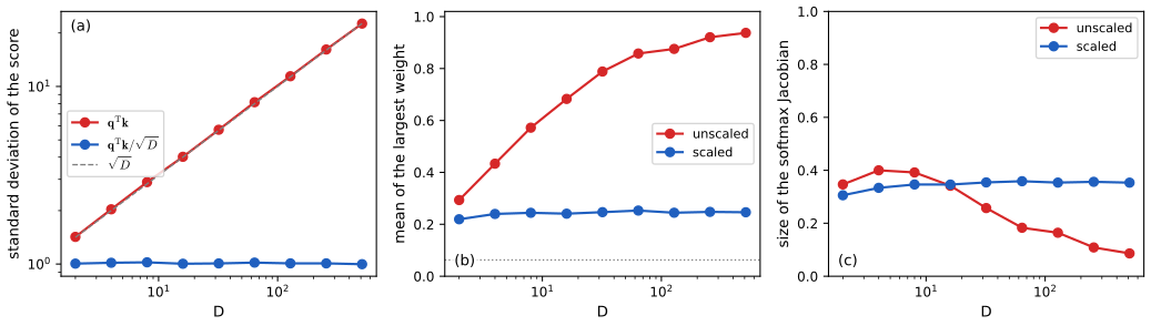
p. 366 Like the logistic sigmoid, the softmax has gradients that become exponentially small when its inputs are large. If the elements of the queries and keys were independent with mean 0 and variance 1, the dot product would have variance \(D_k\) (Exercise 12.4), so the scores are divided by their standard deviation \(\sqrt{D_k}\):
\[ \bY=\Attn(\bQ,\bK,\bV)\equiv\Softmax\left[\frac{\bQ\bK^\T}{\sqrt{D_k}}\right]\bV. \tag{12.14} \]This is scaled dot-product self-attention, one attention head (Figure 12.6, Algorithm 12.1).
Algorithm 12.1 (scaled dot-product self-attention) p. 367
- Input: tokens \(\bX\in\R^{N\times D}\); weights \(\bW^{(q)},\bW^{(k)}\in\R^{D\times D_k}\), \(\bW^{(v)}\in\R^{D\times D_v}\).
- \(\bQ=\bX\bW^{(q)}\), \(\bK=\bX\bW^{(k)}\) (both \(N\times D_k\)), \(\bV=\bX\bW^{(v)}\) (\(N\times D_v\); the book prints \(N\times D\)).
- Return \(\Softmax[\bQ\bK^\T/\sqrt{D_k}]\,\bV\in\R^{N\times D_v}\).
Result 12.2 (the softmax Jacobian, and why saturation stops learning) p. 366
For \(\ba=\Softmax(\bz)\in\R^N\) (one row),
\[ \frac{\partial a_i}{\partial z_j}=a_i(\delta_{ij}-a_j),\qquad\bJ=\diag(\ba)-\ba\ba^\T. \]\(\bJ\) is symmetric and positive semi-definite, \(\bJ\one=\bzero\), and its largest absolute row sum is \(\max_i2a_i(1-a_i)\). If the largest weight is \(1-\varepsilon\), then \(\|\bJ\|_2\le\|\bJ\|_\infty\le2\varepsilon\). For scores \(c\bz\) whose maximum exceeds the next largest score by a gap \(g>0\), \(\varepsilon\le(N-1)e^{-cg}\): the gradient through the softmax vanishes exponentially as the scores grow.
Proof
\(\ln a_i=z_i-\ln\sum_ke^{z_k}\), so \(\partial\ln a_i/\partial z_j=\delta_{ij}-e^{z_j}/\sum_ke^{z_k}=\delta_{ij}-a_j\), and multiplying by \(a_i\) gives the formula. Symmetry is visible. For any \(\bv\), \(\bv^\T\bJ\bv=\sum_ia_iv_i^2-(\sum_ia_iv_i)^2\), the variance of \(v_I\) when the index \(I\) is drawn with probabilities \(\ba\); so \(\bJ\succeq0\), with \(\bv^\T\bJ\bv=0\) for constant \(\bv\), i.e. \(\bJ\one=\ba-\ba(\one^\T\ba)=\bzero\) (adding a constant to all scores changes nothing). Row \(i\): \[\sum_j|J_{ij}|=a_i(1-a_i)+a_i\sum_{j\ne i}a_j=2a_i(1-a_i).\] If \(a_{i^\star}=1-\varepsilon\), then \(2a_{i^\star}(1-a_{i^\star})\le2\varepsilon\), and every other \(a_i\le\varepsilon\) gives \(2a_i(1-a_i)\le2\varepsilon\); so \(\|\bJ\|_\infty\le2\varepsilon\), and for a symmetric matrix \(\|\bJ\|_2\le\sqrt{\|\bJ\|_1\|\bJ\|_\infty}=\|\bJ\|_\infty\). Finally \(\varepsilon\) is bounded as in Filling the gap 12.1 with \(1/T\) replaced by \(c\). A direct computation confirms the Jacobian against finite differences and the row-sum formula. (Companion course: Section 4.3.4 derives the same Jacobian for multiclass logistic regression.)
Result 12.3 (the backward pass of attention) pp. 364–366
Let \(\bS=c\,\bQ\bK^\T\) with \(c=1/\sqrt{D_k}\), \(\bA=\Softmax[\bS]\), \(\bY=\bA\bV\), and let \(\bG=\partial E/\partial\bY\) for a scalar error \(E\). Then, with \(\circ\) the element-wise product,
\[ \frac{\partial E}{\partial\bV}=\bA^\T\bG,\quad\frac{\partial E}{\partial\bA}=\bG\bV^\T,\quad\frac{\partial E}{\partial S_{nm}}=a_{nm}\Big(\frac{\partial E}{\partial a_{nm}}-\sum_{m'}a_{nm'}\frac{\partial E}{\partial a_{nm'}}\Big),\quad\frac{\partial E}{\partial\bQ}=c\,\frac{\partial E}{\partial\bS}\bK,\quad\frac{\partial E}{\partial\bK}=c\Big(\frac{\partial E}{\partial\bS}\Big)^{\!\T}\bQ. \]The cost is \(O(N^2D_k+N^2D_v)\), the same order as the forward pass. Masked entries (\(a_{nm}=0\)) receive no gradient.
Proof
\(Y_{nj}=\sum_ma_{nm}V_{mj}\), so \(\partial E/\partial V_{mj}=\sum_nG_{nj}a_{nm}=(\bA^\T\bG)_{mj}\) and \(\partial E/\partial a_{nm}=\sum_jG_{nj}V_{mj}=(\bG\bV^\T)_{nm}\). Row \(n\) of \(\bA\) depends only on row \(n\) of \(\bS\), through the Jacobian of Result 12.2: \(\partial E/\partial S_{nm}=\sum_k(\partial E/\partial a_{nk})a_{nk}(\delta_{km}-a_{nm})\), which is the stated expression. Finally \(S_{nm}=c\sum_iQ_{ni}K_{mi}\) gives \(\partial E/\partial Q_{ni}=c\sum_m(\partial E/\partial S_{nm})K_{mi}\) and \(\partial E/\partial K_{mi}=c\sum_n(\partial E/\partial S_{nm})Q_{ni}\). If \(a_{nm}=0\) the factor \(a_{nm}\) kills \(\partial E/\partial S_{nm}\). The gradients with respect to the weight matrices follow by one more step, e.g. \(\partial E/\partial\bW^{(q)}=\bX^\T\partial E/\partial\bQ\). A direct computation compares all three against automatic differentiation (difference \(2\times10^{-16}\)). (Companion course: backpropagation in Section 5.3.)
Result 12.4 (the variance of a dot product, and what the scaling achieves) p. 366; Exercise 12.4
If \(\bq,\bkk\in\R^{D}\) are independent, each with uncorrelated components of mean 0 and variance 1, then \(\E[\bq^\T\bkk]=0\) and \(\E[(\bq^\T\bkk)^2]=\var[\bq^\T\bkk]=D\). Gaussianity is not needed. Hence \(\bq^\T\bkk/\sqrt{D}\) has variance 1 whatever \(D\), whereas unscaled scores have standard deviation \(\sqrt{D}\), so that for large \(D\) the softmax saturates and, by Result 12.2, passes almost no gradient.
Proof and discussion
\(\E[\bq^\T\bkk]=\sum_i\E[q_i]\E[k_i]=0\) by independence, and \[ \E[(\bq^\T\bkk)^2]=\sum_{i,j}\E[q_iq_j]\,\E[k_ik_j]=\sum_{i,j}\delta_{ij}\delta_{ij}=D. \] When does the assumption hold? It describes a network at initialisation. Suppose the input of the attention layer has been layer-normalised (Section 7.4.3), so that \(\|\bx\|^2=D\), and \(W^{(q)}_{ij}\) are independent \(\N(0,1/D)\). Then \(q_j=\sum_ix_iW^{(q)}_{ij}\) has mean 0 and variance \(\|\bx\|^2/D=1\), as assumed (the same variance argument as for initialisation in Section 7.2.5). What saturation looks like. Figure 12.S1 draws one query and 16 keys with \(\N(0,\bI)\) entries: unscaled, the mean largest weight rises from 0.29 at \(D=2\) to 0.94 at \(D=512\) and the Jacobian size of Result 12.2 falls from 0.35 to 0.09; scaled, the score spread stays at 1.00 and the largest weight at about 0.25 for every \(D\). A direct computation confirms \(\E[(\bq^\T\bkk)^2]=D\) by Monte Carlo for Gaussian and for random-sign entries.
12.1.6 Multi-head attention
pp. 366–368 One head produces one pattern of weights per token; several relations (grammatical agreement, reference, topic) may matter at once, and a single head would average over them. So \(H\) heads, identical in form but with their own parameters, run in parallel, as a convolutional layer runs several filters:
\[ \bH_h=\Attn(\bQ_h,\bK_h,\bV_h), \tag{12.15} \] \[ \bQ_h=\bX\bW^{(q)}_h, \tag{12.16} \] \[ \bK_h=\bX\bW^{(k)}_h, \tag{12.17} \] \[ \bV_h=\bX\bW^{(v)}_h, \tag{12.18} \] \[ \bY(\bX)=\Concat[\bH_1,\dots,\bH_H]\,\bW^{(o)}. \tag{12.19} \]Each \(\bH_h\) is \(N\times D_v\), the concatenation is \(N\times HD_v\), and \(\bW^{(o)}\in\R^{HD_v\times D}\) brings the result back to \(N\times D\) (Figures 12.7, 12.8). The usual choice is \(D_k=D_v=D/H\).
Algorithm 12.2 (multi-head attention, typographical errors corrected) p. 368
- Input: \(\bX\in\R^{N\times D}\); for \(h=1,\dots,H\): \(\bW^{(q)}_h,\bW^{(k)}_h\in\R^{D\times D_k}\) (the book prints \(D\times D\)), \(\bW^{(v)}_h\in\R^{D\times D_v}\); \(\bW^{(o)}\in\R^{HD_v\times D}\).
- For \(h=1,\dots,H\): \(\bQ_h=\bX\bW^{(q)}_h\), \(\bK_h=\bX\bW^{(k)}_h\), \(\bV_h=\bX\bW^{(v)}_h\); \(\bH_h=\Attn(\bQ_h,\bK_h,\bV_h)\in\R^{N\times D_v}\) (Algorithm 12.1).
- \(\bH=\Concat[\bH_1,\dots,\bH_H]\) (the book prints \(\bH_N\) as the last block).
- Return \(\bY=\bH\bW^{(o)}\in\R^{N\times D}\), with rows \(\by_1,\dots,\by_N\) (the book prints \(\bx_N\) as the last one).
Result 12.5 (multi-head attention is a sum of low-rank heads) p. 368; Exercise 12.5, corrected
Split \(\bW^{(o)}\) into \(H\) blocks of rows, \(\bW^{(o)}=[\bW^{(o)}_1;\dots;\bW^{(o)}_H]\) with \(\bW^{(o)}_h\in\R^{D_v\times D}\), and let \(\bA_h=\Softmax[\bQ_h\bK_h^\T/\sqrt{D_k}]\) be the \(N\times N\) weight matrix of head \(h\). Then
\[ \bY=\sum_{h=1}^H\bA_h\,\bX\,\bW^{(h)},\qquad\bW^{(h)}=\bW^{(v)}_h\bW^{(o)}_h\in\R^{D\times D},\qquad\rank\bW^{(h)}\le D_v. \]Erratum. The book's (12.42) writes \(\bH_h\bX\bW^{(h)}\) with \(\bH_h\) "given by (12.15)"; but (12.15) defines \(\bH_h=\bA_h\bV_h\), an \(N\times D_v\) matrix, which cannot multiply the \(N\times D\) matrix \(\bX\) (unless \(D_v=N\)). The factor must be the weight matrix \(\bA_h\).
Proof
Block multiplication: \(\Concat[\bH_1,\dots,\bH_H]\bW^{(o)}=\sum_h\bH_h\bW^{(o)}_h\), since column block \(h\) of the left factor meets row block \(h\) of the right one. Then \(\bH_h=\bA_h\bV_h=\bA_h\bX\bW^{(v)}_h\) gives the formula, and \(\rank(\bW^{(v)}_h\bW^{(o)}_h)\le\min(\rank\bW^{(v)}_h,\rank\bW^{(o)}_h)\le D_v\). With \(D_v=D/H\) each \(\bW^{(h)}\) is rank-deficient, so replacing it by an unrestricted \(D\times D\) matrix would change the model (and cost \(HD^2\) instead of \(2DD_v H=2D^2\) parameters). A direct computation confirms the identity, the dimension clash of the printed form and the ranks.
12.1.7 Transformer layers
See also layer normalisation in Section 7.4.3, and the product of layer Jacobians in Filling the gap 7.8.
pp. 368–370 To stack layers, each multi-head block gets a residual connection (Section 9.5) and layer normalisation (Ba, Kiros and Hinton, 2016):
\[ \bZ=\LN[\bY(\bX)+\bX], \tag{12.20} \]or, in the pre-norm variant that often optimises better,
\[ \bZ=\bY(\bX')+\bX,\quad\text{where}\quad\bX'=\LN[\bX]. \tag{12.21} \]The attention outputs are linear combinations of linearly transformed inputs; to add nonlinear processing of the features, a shared MLP with \(D\) inputs and outputs (for example two layers with ReLU hidden units) is applied to every row, again with a residual connection and normalisation:
\[ \widetilde\bX=\LN[\MLP[\bZ]+\bZ], \tag{12.22} \] \[ \widetilde\bX=\MLP(\bZ')+\bZ,\quad\text{where}\quad\bZ'=\LN[\bZ]. \tag{12.23} \]Algorithm 12.3 (transformer layer) p. 371
- Input: \(\bX\in\R^{N\times D}\); multi-head attention parameters; MLP parameters.
- \(\bZ=\LN[\bY(\bX)+\bX]\), with \(\bY\) from Algorithm 12.2.
- \(\widetilde\bX=\LN[\MLP[\bZ]+\bZ]\), the MLP acting on each row with shared weights.
- Return \(\widetilde\bX\in\R^{N\times D}\). (Pre-norm: replace the two lines by (12.21) and (12.23).)
Filling the gap 12.3: what attention alone cannot do, and why the MLP is there p. 369
Derivation
For one head, by Result 12.5, \(\by_n=\bW^{(h)\T}\sum_ma_{nm}\bx_m\): every output is a fixed linear map applied to a convex combination of the inputs. So the outputs lie in \(\bW^{(h)\T}\operatorname{span}\{\bx_1,\dots,\bx_N\}\), a space of dimension at most \(\min(N,D_v)\) (the book says "the subspace spanned by the input vectors", which is exact only when \(\bW^{(h)}=\bI\)); with \(H\) heads, in the sum of \(H\) such spaces. If two tokens have the same weights, they get the same output. The only nonlinearity is in the weights \(a_{nm}\). In particular attention cannot apply a nonlinear function to the features of a single token: for \(N=1\) the weight is 1 and the layer is linear, \(\by_1=\bW^{(h)\T}\bx_1\). The position-wise MLP supplies this, and as it acts on each row separately it does not depend on \(N\). A direct computation confirms that the rows of \(\bA\bX\) lie in the 7-dimensional span of 7 inputs in \(\R^{12}\).
Filling the gap 12.4: residual connections, and where to put the normalisation pp. 369–370, (12.20)–(12.23)
The book says pre-norm "can result in more effective optimization". Here is the structural reason, in terms of Jacobians.
Derivation
Write one sub-layer (attention or MLP) as \(F_l\) and follow one token, \(\bx^{(l)}\in\R^D\) (the argument is the same for the whole matrix). Pre-norm: \(\bx^{(l+1)}=\bx^{(l)}+F_l(\LN(\bx^{(l)}))\), so \[ \bx^{(L)}=\bx^{(0)}+\sum_{l=0}^{L-1}F_l\big(\LN(\bx^{(l)})\big),\qquad\frac{\partial\bx^{(L)}}{\partial\bx^{(0)}}=\prod_{l}\Big(\bI+\frac{\partial F_l(\LN(\bx^{(l)}))}{\partial\bx^{(l)}}\Big). \] Expanding the product gives \(\bI\) plus terms each involving at least one sub-layer: the error at the output reaches every layer through an identity path that no weight matrix or normalisation touches. Post-norm: \(\bx^{(l+1)}=\LN(\bx^{(l)}+F_l(\bx^{(l)}))\), so every path back to \(\bx^{(0)}\), the residual one included, passes through all \(L\) layer-norm Jacobians. By Result 7.11, \(\partial\LN(\bu)/\partial\bu=\frac1\sigma(\bI-\frac1D\one\one^\T-\frac1D\widehat\bu\widehat\bu^\T)\) with \(\sigma\) the standard deviation of the components of \(\bu\) and \(\widehat\bu\) its normalised version: a projection divided by \(\sigma\). As the residual sums grow, \(\sigma>1\) and the product of \(L\) such factors shrinks the gradients reaching the early layers, which is why post-norm transformers usually need a learning-rate warm-up (Xiong et al., 2020). In both forms the normalisation keeps each token's features at a fixed mean and scale (pre-norm: at the input of every sub-layer), so that the variance argument of Result 12.4 applies in every layer. Our character model (Section 12.3.1) is pre-norm with a final layer norm before the output; the vision transformer of Figure 12.S7 is post-norm. A numerical experiment runs both forms of Algorithm 12.3 and confirms that post-norm outputs have mean 0 and variance 1 in every row.
12.1.8 Computational complexity
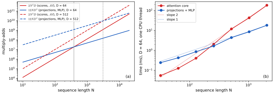
pp. 370–371 A fully connected map from the \(ND\) inputs to the \(ND\) outputs would have \(O(N^2D^2)\) weights and cost. Attention shares \(\bW^{(q)},\bW^{(k)},\bW^{(v)}\) across tokens, so it has \(O(D^2)\) parameters; the dot products cost \(O(N^2D)\) and the shared MLP \(O(ND^2)\). Which term dominates depends on \(N\) and \(D\).
Result 12.6 (parameters of a layer; Exercise 12.16) pp. 368, 370; Exercise 12.16
With biases and \(D_k=D_v=D/H\), multi-head attention has \(4D^2+4D\) parameters, whatever \(H\). A layer of Algorithm 12.3 with MLP width \(D_{\rm ff}\) has
\[ \underbrace{4D^2+4D}_{\text{attention}}+\underbrace{2DD_{\rm ff}+D_{\rm ff}+D}_{\text{MLP}}+\underbrace{4D}_{\text{two layer norms}}=12D^2+13D\quad(D_{\rm ff}=4D). \]For BERT-Large (\(D=1024\), 24 layers, 16 heads of size 64, \(D_{\rm ff}=4096\), 30 000 tokens, 512 positions) this gives 302.3 million in the layers, 31.2 million in the embeddings and 1.0 million in the output "pooler": 334.6 million, the "approximately 340 million" of the exercise.
Proof
Per head: \(\bW^{(q)}_h,\bW^{(k)}_h\) have \(DD_k\) entries each and \(\bW^{(v)}_h\) has \(DD_v\), plus \(2D_k+D_v\) biases; \(\bW^{(o)}\) has \(HD_vD\) entries and \(D\) biases. With \(D_k=D_v=D/H\): \(H\cdot3D\cdot\frac DH+D^2=4D^2\) weights and \(3D+D=4D\) biases. The MLP has \(D\times D_{\rm ff}\) and \(D_{\rm ff}\times D\) weights and \(D_{\rm ff}+D\) biases; each layer norm a gain and a shift of length \(D\). BERT-Large: per layer \(12\cdot1024^2+13\cdot1024=12\,596\,224\), times 24 is \(302\,309\,376\); embeddings: tokens \(30\,000\times1024\), positions \(512\times1024\), two segment vectors and one layer norm, \(31\,248\,384\); pooler \(1024^2+1024\). Total \(334\,607\,360\). (The published model has 30 522 tokens, which adds 0.5 million.) A direct computation confirms the per-layer count against PyTorch's own transformer layer.
Result 12.7 (cost of a layer, and Exercise 12.6) pp. 370–371; Exercise 12.6
A forward pass through one layer costs, in multiply-adds,
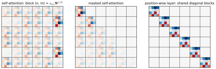
\[ \underbrace{2N^2D}_{\bQ_h\bK_h^\T\ \text{and}\ \bA_h\bV_h\ \text{over all heads}}+\underbrace{4ND^2}_{\text{four projections}}+\underbrace{2NDD_{\rm ff}}_{\text{MLP}}=2N^2D+12ND^2\quad(D_{\rm ff}=4D), \]and stores \(HN^2\) attention weights. The two terms are equal at \(N=6D\); above it the quadratic term dominates. As a map from \(\vecop(\bX)\in\R^{ND}\) (rows stacked) to \(\vecop(\bY)\), one head is the \(ND\times ND\) matrix
\[ \vecop(\bY)=\big(\bA\otimes\bW^{(v)\T}\big)\vecop(\bX),\qquad\text{block }(n,m)=a_{nm}\bW^{(v)\T}, \]while the position-wise MLP's first layer is \(\bI_N\otimes\bW_1^\T\), block-diagonal with identical blocks (Figure 12.S8).
Proof
Scores: head \(h\) forms \(N^2\) dot products of length \(D/H\), so \(N^2D\) over the heads; the product \(\bA_h\bV_h\) is another \(N^2D/H\) per head. The projections are four products of an \(N\times D\) matrix with \(D\times D\) matrices; the MLP has two products of sizes \(N\times D\times D_{\rm ff}\). With \(D_{\rm ff}=4D\): \(2N^2D=12ND^2\iff N=6D\). For the Kronecker form, \(\by_n=\sum_ma_{nm}\bW^{(v)\T}\bx_m\), which is row \(n\) of block row \(n\) applied to the stacked inputs. In a fully connected layer every block would be an independent \(D\times D\) matrix: \(N^2D^2\) parameters. Here all blocks are multiples of one shared matrix, with multipliers computed from the data; with the causal mask (Section 12.3.1) the blocks above the diagonal are zero. Figure 12.S3 confirms the scaling by timing: on one CPU thread at \(D=64\), the attention core grows like \(N^{1.97}\) and the per-token parts like \(N^{1.03}\), crossing near \(N=256\) (the flop crossover is \(6D=384\); the constants of the two kinds of matrix product differ). A direct computation confirms the Kronecker identity exactly.
12.1.9 Positional encoding
See also the companion course on high-dimensional geometry, Section 1.4, and Section 6.1.2 of this course; and equivariance of convolutions in Section 5.5.6 of the companion course.
pp. 371–372 All weights of a layer are shared across tokens, so reordering the input rows only reorders the output rows: a transformer is equivariant to permutations (Exercise 12.7). That is what makes it parallel and lets it relate distant tokens as easily as near ones, but it also means that "The food was bad, not good at all." and "The food was good, not bad at all." are processed as the same set. Order must be put into the data.
Result 12.8 (permutation equivariance, and what breaks it) p. 371; Exercise 12.7
Let \(\bP\) be an \(N\times N\) permutation matrix. (i) For row-wise softmax and any permutations \(\bP\), \(\bP'\): \(\Softmax[\bP\bS\bP'^\T]=\bP\,\Softmax[\bS]\,\bP'^\T\). (ii) Multi-head self-attention (12.19), the residual connections, layer normalisation and the position-wise MLP all satisfy \(f(\bP\bX)=\bP f(\bX)\), hence so does a stack of transformer layers. (iii) A causal mask \(\bM\) and added position encodings \(\bR\) break this: \(f\) is then equivariant only to permutations with \(\bP\bM\bP^\T=\bM\) (only the identity, for the causal mask) or \(\bP\bR=\bR\).
Proof
(i) Permuting the rows of \(\bS\) permutes which row is normalised, not how; permuting the entries within a row permutes the exponentials and leaves their sum, the normaliser, unchanged. (ii) For \(\bX\mapsto\bP\bX\): \(\bQ_h\mapsto\bP\bQ_h\), \(\bK_h\mapsto\bP\bK_h\), \(\bV_h\mapsto\bP\bV_h\), so the scores become \(\bP\bQ_h\bK_h^\T\bP^\T\), the weights \(\bP\bA_h\bP^\T\) by (i), and the head output \(\bP\bA_h\bP^\T\bP\bV_h=\bP\bA_h\bV_h\) since \(\bP^\T\bP=\bI\). Concatenation and the right multiplication by \(\bW^{(o)}\) act on columns and commute with \(\bP\). The residual sum \(\bP\bY+\bP\bX=\bP(\bY+\bX)\). Layer norm and the MLP act on each row with the same function, so permuting rows before or after gives the same result. A composition of equivariant maps is equivariant. (iii) With a mask, the scores are \(\bP\bS\bP^\T+\bM\), while equivariance needs \(\bP(\bS+\bM)\bP^\T\); these agree for all \(\bS\) iff \(\bP\bM\bP^\T=\bM\). For the causal mask this means \(\bP\) preserves the order of positions, so \(\bP=\bI\). With encodings, the input becomes \(\bP\bX+\bR\) instead of \(\bP(\bX+\bR)\). A direct computation confirms (ii) to \(10^{-12}\) for both forms of the layer, and errors of 2.3 and 0.8 for (iii).
pp. 372–373 A position-encoding vector \(\br_n\) is added to the token at position \(n\), rather than concatenated (which would enlarge every later space):
\[ \widetilde\bx_n=\bx_n+\br_n. \tag{12.24} \]This might seem to corrupt the token, but random vectors in high dimension are nearly orthogonal (Exercise 12.8), residual connections carry the encoding through all layers, and under the linear maps that follow, adding is equivalent to concatenating (Exercise 12.9).
Filling the gap 12.5: random directions are nearly orthogonal, and adding is concatenating p. 372; Exercises 12.8, 12.9
Derivation
Near-orthogonality. Let \(\ba,\bb\) be independent unit vectors in \(\R^D\), each with a distribution invariant under rotations. Condition on \(\bb\) and rotate the coordinates (an orthonormal basis \(\{\bu_i\}\) with \(\bu_1=\bb\)): by invariance the distribution of \(\ba\) does not change, and \(\cos\theta=\ba^\T\bb=a_1\), the first coordinate. Since \(\sum_ia_i^2=1\) and all coordinates have the same distribution by symmetry, \(\E[a_1^2]=1/D\). Hence \(\E[\cos\theta]=0\) (by the symmetry \(\ba\mapsto-\ba\)), \(\E[\cos^2\theta]=1/D\), and by Chebyshev's inequality \(P(|\cos\theta|>t)\le1/(Dt^2)\). For \(D=512\) the typical \(|\cos\theta|\) is about \(1/\sqrt{512}=0.044\) (Monte Carlo: \(\E[\cos^2\theta]=0.00196\) against \(1/512=0.00195\)). So a learned token direction and a position direction interfere little, and a later linear map can read either with little cross-talk. (Exact distribution: \(a_1^2\sim\mathrm{Beta}(\frac12,\frac{D-1}2)\). Companion course: Section 1.4.)
Concatenation versus addition. For any matrix \(\bW=[\bW_x\ \bW_e]\) acting on a concatenation, \(\bW\begin{pmatrix}\bx\\\be\end{pmatrix}=\bW_x\bx+\bW_e\be\): the result is the sum of a transformed token and a transformed position. Conversely, adding is concatenating followed by \(\bW=[\bI\ \bI]\). Since every token enters a transformer through linear maps (\(\bW^{(q)},\bW^{(k)},\bW^{(v)}\), and the first MLP layer), an additive encoding of dimension \(D\) can do what a concatenated one does, without enlarging \(D\); the price is that the learned maps share the same \(D\) dimensions between content and position.
pp. 372–374 A good encoding should be unique for each position, bounded, defined for sequences longer than those seen in training, and should express the offset between two positions in the same way wherever they are. Integers \(1,2,3,\dots\) are unbounded; fractions \(n/N\) depend on the length. The sinusoidal encoding of Vaswani et al. (2017) satisfies all four requirements:
\[ r_{ni}=\begin{cases}\sin\Big(\dfrac{n}{L^{i/D}}\Big),&i\text{ even},\\[2mm]\cos\Big(\dfrac{n}{L^{(i-1)/D}}\Big),&i\text{ odd},\end{cases} \tag{12.25} \]with components \(i=0,\dots,D-1\): pairs (sine, cosine) at angular frequencies \(\omega_j=L^{-2j/D}\), \(j=0,\dots,D/2-1\), from 1 down to nearly \(1/L\), like the bits of a binary counter but continuous (p. 374). Vaswani et al. use \(L=10\,000\); the book's figure uses \(L=30\).
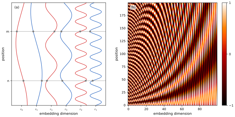
Result 12.9 (relative positions are rotations) p. 374; Exercise 12.10
Let \(\br_n\) be given by (12.25) with distinct frequencies \(\omega_j\in(0,\pi)\). Then:
- For every offset \(k\), \(\br_{n+k}=\bM(k)\br_n\) for all \(n\), with \(\bM(k)\) block-diagonal with \(2\times2\) blocks \[\begin{pmatrix}\cos\omega_jk&\sin\omega_jk\\-\sin\omega_jk&\cos\omega_jk\end{pmatrix},\] rotations that depend on \(k\) only.
- \(\bM(k)\) is orthogonal, \(\bM(j)\bM(k)=\bM(j+k)\), \(\bM(-k)=\bM(k)^\T\); hence \(\|\br_n\|^2=D/2\) for all \(n\) and every component is in \([-1,1]\).
- \(\br_n^\T\br_m=\sum_j\cos(\omega_j(n-m))\) depends on \(n-m\) only.
- Distinct integer positions have distinct encodings.
- With sines only, no matrix \(\bM\) maps \(\br_n\) to \(\br_{n+k}\) for all \(n\) (unless every \(\sin\omega_jk=0\)).
- A head with \(\bW^{(q)}\bW^{(k)\T}=\bM(k)\) acting on the encodings gives the score \(\br_n^\T\bM(k)\br_m=\br_{n-k}^\T\br_m\), largest at \(m=n-k\): the same weight matrix attends "\(k\) places back" at every position.
Proof (Exercise 12.10 and the rest)
1. By (12.44) and (12.45), \(\sin(\omega(n+k))=\cos\omega k\,\sin\omega n+\sin\omega k\,\cos\omega n\) and \[\cos(\omega(n+k))=-\sin\omega k\,\sin\omega n+\cos\omega k\,\cos\omega n,\] which is the stated \(2\times2\) block acting on \((\sin\omega n,\cos\omega n)\); the coefficients involve \(k\) only. This needs both the sine and the cosine of each frequency.
2. Each block is a rotation (orthogonal, determinant 1) by the angle \(-\omega_jk\); rotation angles add, and reversing the angle transposes. So \(\|\br_n\|=\|\bM(n)\br_0\|=\|\br_0\|\), and \(\br_0=(0,1,0,1,\dots)\) has \(\|\br_0\|^2=D/2\).
3. \[\br_n^\T\br_m=\sum_j[\sin\omega_jn\sin\omega_jm+\cos\omega_jn\cos\omega_jm]=\sum_j\cos(\omega_j(n-m)).\]
4. If \(\br_n=\br_m\), the first pair (\(\omega_0=1\)) gives \(\sin n=\sin m\) and \(\cos n=\cos m\), so \(n-m\in2\pi\mathbb{Z}\); for integers this forces \(n=m\) because \(\pi\) is irrational.
5. Suppose \(\sin(\omega_j(n+k))=\sum_iM_{ji}\sin(\omega_in)\) for all integers \(n\ge0\). At \(n=0\) the right side vanishes, so \(\sin\omega_jk=0\) for all \(j\). (Without position 0, the same conclusion follows because the sequences \(\sin\omega_in\), \(\cos\omega_in\) are linearly independent for distinct \(\omega_i\in(0,\pi)\), being combinations of the distinct geometric sequences \(e^{\pm\mathrm{i}\omega_in}\), and \(\sin(\omega_j(n+k))\) has the non-zero cosine coefficient \(\sin\omega_jk\).)
6. \[\br_n^\T\bM(k)\br_m=(\bM(k)^\T\br_n)^\T\br_m=(\bM(-k)\br_n)^\T\br_m=\br_{n-k}^\T\br_m,\] and by Cauchy–Schwarz and part 2 this is at most \(D/2\), with equality iff \(\br_m=\br_{n-k}\), i.e. \(m=n-k\) by part 4. This is the precise sense of the book's "the network should be able to learn to attend to relative positions"; rotary position embeddings (Su et al., 2021) build the same rotation into the queries and keys directly. A direct computation confirms 1–3 to \(10^{-12}\) for \(D=64\), \(L=10\,000\), and that the best least-squares map for sines only leaves a 40% relative residual.
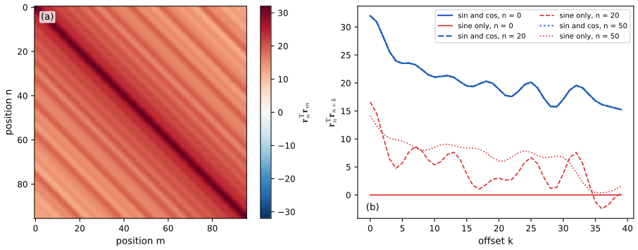
p. 374 The alternative is a learned encoding, a free vector per position trained with the rest of the model. It needs no design, but positions never seen in training have untrained vectors, so it suits inputs of fixed length (as in the vision transformers of Section 12.4.1).
12.2 Natural language
pp. 374–375 Text is a sequence of words and punctuation. The first task is to represent it numerically. A one-hot vector of length \(K\), the size of a dictionary, has a 1 in the position of its word; it is huge (\(K\) is in the hundreds of thousands) and says nothing about which words are related. Both problems are solved by mapping words to dense vectors of a few hundred dimensions.
12.2.1 Word embedding
pp. 375–376 An embedding matrix \(\bE\in\R^{D\times K}\) maps a one-hot \(\bx_n\) to
\[ \bv_n=\bE\bx_n, \tag{12.26} \]which is simply the column of \(\bE\) for that word: an embedding layer is a table lookup, implemented as such. word2vec (Mikolov et al., 2013) learns \(\bE\) with a two-layer linear network from windows of \(M\) consecutive words (Figure 12.11): the continuous bag of words predicts the centre word from its neighbours, skip-grams predict the neighbours from the centre word. This is self-supervised: the labels are words of the text itself. Related words end up close, because they occur in similar contexts, and the space shows linear regularities such as
\[ \bv(\text{Paris})-\bv(\text{France})+\bv(\text{Italy})\simeq\bv(\text{Rome}). \tag{12.27} \]Today embeddings are the first layer of a deep network, fixed from pre-training or trained end to end.
Result 12.10 (what skip-gram embeddings learn) pp. 375–376, (12.27)
Skip-gram with negative sampling maximises, over word vectors \(\bv_w\) and context vectors \(\bu_c\),
\[ \ell=\sum_{(w,c)}\Big[\ln\sigma(\bu_c^\T\bv_w)+k\,\E_{c'\sim P_n}\ln\sigma(-\bu_{c'}^\T\bv_w)\Big], \]the sum running over all (centre, context) pairs in the corpus, with \(k\) negative contexts drawn from the unigram distribution \(P_n(c)=\#(c)/|\mathcal{D}|\). If the dimension is large enough for the scores \(x_{wc}=\bu_c^\T\bv_w\) to be chosen freely, the maximiser is
\[ \bu_c^\T\bv_w=\ln\frac{\#(w,c)\,|\mathcal{D}|}{\#(w)\,\#(c)}-\ln k=\PMI(w,c)-\ln k, \]the pointwise mutual information of word and context, shifted by \(\ln k\) (Levy and Goldberg, 2014). The analogy (12.27) then holds whenever the context ratios match, \[p(c\given\text{Paris})/p(c\given\text{France})\approx p(c\given\text{Rome})/p(c\given\text{Italy})\] for all contexts \(c\), and the context vectors span the space.
Proof
Collect the terms of \(\ell\) that involve the score \(x=x_{wc}\) of one pair: the positive term occurs \(\#(w,c)\) times, and \(c\) is drawn as a negative for \(w\) on average \(k\#(w)P_n(c)=k\#(w)\#(c)/|\mathcal{D}|\) times. So \(\ell\) contains \[ f(x)=A\ln\sigma(x)+B\ln\sigma(-x),\qquad A=\#(w,c),\ B=\frac{k\#(w)\#(c)}{|\mathcal{D}|}. \] Using \(\frac{\d}{\d x}\ln\sigma(x)=\sigma(-x)\): \[f'(x)=A\sigma(-x)-B\sigma(x)=0\iff e^x=\sigma(x)/\sigma(-x)=A/B,\] and \(f''(x)=-(A+B)\sigma(x)\sigma(-x)<0\), so \(x^\star=\ln(A/B)\) is the unique maximum, which is the stated formula; with free scores each pair is maximised separately. For the analogy: \(\PMI(w,c)=\ln p(c\given w)-\ln p(c)\), so \[ (\bv_{\rm Paris}-\bv_{\rm France}-\bv_{\rm Rome}+\bv_{\rm Italy})^\T\bu_c=\ln\frac{p(c\given\text{Paris})\,p(c\given\text{Italy})}{p(c\given\text{France})\,p(c\given\text{Rome})}, \] the shifts \(-\ln p(c)-\ln k\) cancelling. If the ratio is close to 1 for every context, the vector in brackets is nearly orthogonal to all \(\bu_c\), hence nearly zero when the \(\bu_c\) span \(\R^D\): that is (12.27). A numerical experiment maximises \(f\) numerically on a random count table and recovers \(\PMI-\ln k\) to \(5\times10^{-5}\).
12.2.2 Tokenization
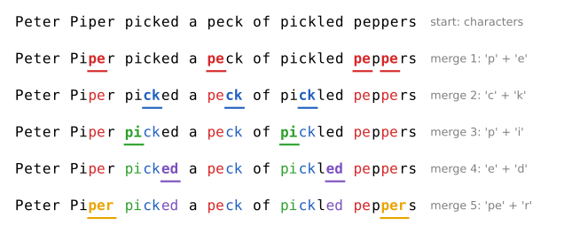
pp. 377–378 A fixed word list cannot handle unknown or misspelled words, punctuation or code; characters handle everything but make sequences long and force the network to rebuild words. Subword tokens sit in between: frequent words become single tokens, rare ones are split into pieces, and related forms ("cook", "cooks", "cooking") share pieces (Schuster and Nakajima, 2012). Byte-pair encoding, a compression method adapted to text by Sennrich, Haddow and Birch (2015), builds the vocabulary by repeated merging.
Algorithm 12.4 (byte-pair encoding) pp. 377–378, Figure 12.12
- Split the training text into words (a merge never crosses white space); start with the vocabulary of single characters and every word as a sequence of characters.
- Count all adjacent pairs of tokens within words. Choose the most frequent pair (ties: here the shorter new token, then the earlier occurrence), add the concatenated token to the vocabulary, and replace every occurrence of the pair, scanning each word from left to right.
- Repeat until the vocabulary has the chosen size. To encode new text, apply the learned merges in the same order.
Filling the gap 12.6: what a merge does to the vocabulary and to the length pp. 377–378
Derivation
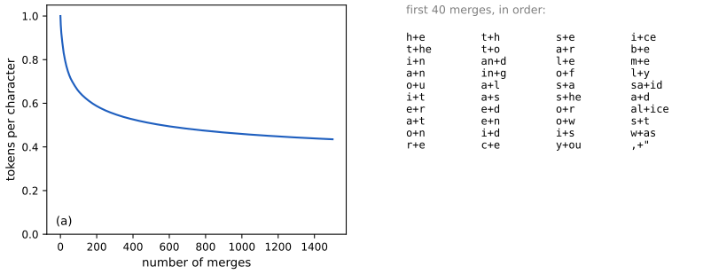
Each merge adds exactly one token to the vocabulary, so after \(r\) merges there are \(K_0+r\) tokens (\(K_0\) characters). Each merge never lengthens a sequence: every replaced occurrence turns two tokens into one, so the length falls by the number of replacements, and concatenating the tokens always gives back the original text (encoding is lossless). The number of replacements can be smaller than the pair count when occurrences overlap: in "eee" the pair (e, e) is counted twice but only one replacement is possible (giving "ee", "e"). A direct computation confirms the counts 4, 3, 2, 2, 2 on the book's sentence, that every row of Figure 12.12 concatenates to the sentence, and the overlap case. On our corpus (the 128 000 training characters of the novel used in Section 12.3.1, 37 distinct characters inside words), 100 merges already cut the length to 0.66 tokens per character, 500 to 0.51 and 1500 to 0.44 (Figure 12.S5): the trade-off between vocabulary size and sequence length that the book describes. The first merges are the commonest bigrams of English ('h'+'e', 't'+'he', 'i'+'n', 'a'+'n', ...).
For the rest of the chapter the book uses words as tokens, for ease of explanation; our trained models use characters, the other extreme, because they are small.
12.2.3 Bag of words
See also the companion course, multinomial variables in Section 2.2 and naive Bayes in Section 4.2.3; and Section 5.3.3 of this course.
pp. 378–379 The simplest model of a sequence treats its tokens as independent draws from one distribution,
\[ p(\bx_1,\dots,\bx_N)=\prod_{n=1}^Np(\bx_n), \tag{12.28} \]a bag of words: order is ignored, and the maximum-likelihood table is the relative frequency of each word (Exercise 12.11). With one such table per class it gives the naive Bayes classifier
\[ p(\bx_1,\dots,\bx_N\given\mathcal{C}_k)=\prod_{n=1}^Np(\bx_n\given\mathcal{C}_k), \tag{12.29} \] \[ p(\mathcal{C}_k\given\bx_1,\dots,\bx_N)\propto p(\mathcal{C}_k)\prod_{n=1}^Np(\bx_n\given\mathcal{C}_k), \tag{12.30} \]e.g. for the sentiment of a review. A word never seen in a class gets probability 0 and vetoes that class, so the tables are smoothed.
Result 12.11 (maximum likelihood for probability tables, and smoothing) pp. 378–379; Exercises 12.11, 12.12
(i) For a shared table \(\pi_1,\dots,\pi_K\) and word counts \(n_1,\dots,n_K\) in a training text of \(N\) tokens, the maximum-likelihood estimate is \(\pi_k=n_k/N\). (ii) For an L-gram table, \(p(x\given\text{context})\) is estimated by \[\#(\text{context},x)/\#(\text{context followed by a token}).\] (iii) Adding \(\alpha\) to every count, \((n_k+\alpha)/(N+K\alpha)\), is the posterior mean of \(\boldsymbol\pi\) under a symmetric Dirichlet\((\alpha)\) prior; \(\alpha=1\) is Laplace's rule. (iv) A general table for \(p(x_n\given x_1,\dots,x_{n-1})\) has \(K^{n-1}(K-1)\) free entries.
Proof
(i) The log-likelihood is \(\sum_kn_k\ln\pi_k\). With a Lagrange multiplier for \(\sum_k\pi_k=1\), \[\partial/\partial\pi_k[\sum_jn_j\ln\pi_j+\lambda(1-\sum_j\pi_j)]=n_k/\pi_k-\lambda=0,\] so \(\pi_k=n_k/\lambda\), and the constraint gives \(\lambda=N\). The objective is concave, so this is the maximum (a word with \(n_k=0\) gets \(\pi_k=0\), on the boundary). (ii) The same argument applied to each context separately, since the likelihood factorises over contexts; the denominator counts only the occurrences of the context that are followed by a token (Exercise 12.13). (iii) With prior \(\propto\prod_k\pi_k^{\alpha-1}\), the posterior is Dirichlet\((n_k+\alpha)\) with mean \((n_k+\alpha)/(N+K\alpha)\) (companion course, Section 2.2.1). (iv) For each of the \(K^{n-1}\) contexts, a distribution over \(K\) values has \(K-1\) free numbers. Summed over \(n=1,\dots,N\), \(\sum_n K^{n-1}(K-1)=K^N-1\), the number of free parameters of a general distribution over \(K^N\) sequences: the chain rule (12.31) by itself saves nothing. For \(K=39\) characters and \(n=4\) already \(2\,254\,122\). A direct computation confirms (i) against perturbed tables. (Lagrange multipliers: companion course toolkit.)
12.2.4 Autoregressive models
See also the companion course, factorising joint distributions in Section 8.1, Markov models in Section 13.1 and hidden Markov models in Section 13.2; and information theory in Section 2.5 of this course.
pp. 379–380 By the product rule, any joint distribution of a sequence factorises as
\[ p(\bx_1,\dots,\bx_N)=\prod_{n=1}^Np(\bx_n\given\bx_1,\dots,\bx_{n-1}), \tag{12.31} \]a fully connected graphical model in which each token depends on all earlier ones. General tables for these conditionals grow exponentially (Result 12.11(iv)), so the dependence is truncated to the last \(L\) tokens; for \(L=2\)
\[ p(\bx_1,\dots,\bx_N)=p(\bx_1)p(\bx_2\given\bx_1)\prod_{n=3}^Np(\bx_n\given\bx_{n-1},\bx_{n-2}), \tag{12.32} \]with the conditional tables shared across positions. \(L=1\) is a bigram model, \(L=2\) a trigram, in general an n-gram model (\(n=L+1\)). All these models can generate text by sampling one token at a time, but with a context of two words the text is incoherent, and \(L\) cannot grow because the tables grow like \(K^L\). A hidden Markov model carries information further through a latent state, but distant tokens still act only through a chain of state updates.
Definition 12.2 (cross-entropy and perplexity per token)
A model \(q\) of sequences, evaluated on a text \(x_1,\dots,x_N\), has cross-entropy per token and perplexity
\[ H_q=-\frac1N\sum_{n=1}^N\ln q(x_n\given x_1,\dots,x_{n-1}),\qquad\PP=e^{H_q}=\Big(\prod_{n=1}^Nq(x_n\given x_{<n})\Big)^{-1/N}. \]The perplexity is the effective number of equally likely choices per token: a uniform model over \(K\) tokens has \(\PP=K\). \(H_q/\ln2\) is the number of bits per token a coder based on \(q\) would need. For a stationary source, \(H_q\) on a long text estimates the source's entropy rate plus the excess (a Kullback–Leibler divergence rate) due to the model, so lower is better and the entropy rate is the floor (Section 2.5.5; companion course Section 1.6). Minimising \(H_q\) on training text is maximum likelihood, the training criterion of every language model in this chapter.
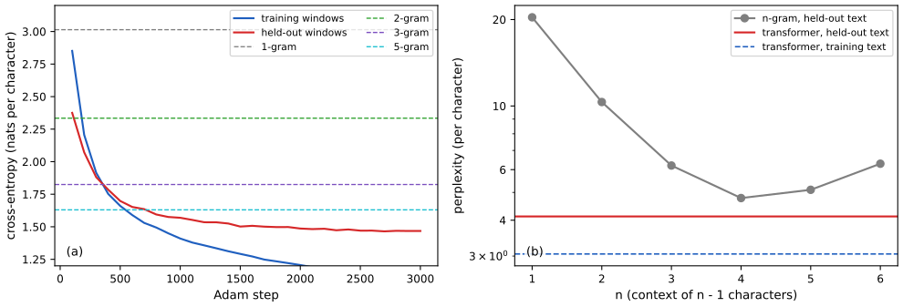
On our character corpus the n-gram models, with add-\(\alpha\) smoothing tuned on held-out text, reach held-out cross-entropies of 3.01 (unigram), 2.33 (bigram), 1.82 (trigram) and 1.56 nats per character (4-gram, perplexity 4.78); longer contexts do worse (1.63 and 1.84 for 5- and 6-grams), because most long contexts are seen too rarely. The small transformer of Section 12.3.1, with a context of 64 characters, reaches 1.42 (perplexity 4.12) (Figure 12.S4).
12.2.5 Recurrent neural networks
pp. 380–381 Parametric models share parameters across positions, handle any length and need far fewer parameters than tables. A recurrent neural network introduces a hidden state \(\bz_n\): a network takes \(\bx_n\) and \(\bz_{n-1}\) and returns an output \(\by_n\) and the new state \(\bz_n\), with the same weights at every step, starting from e.g. \(\bz_0=\bzero\) (Figure 12.13; pseudo-code in Exercise 12.14). For translation (Figure 12.14), the source sentence is read in, a \(\langle\)start\(\rangle\) token triggers the output, and each generated word is fed back as the next input until a \(\langle\)stop\(\rangle\) token: an encoder that compresses the sentence into the state \(\bz^\star\), and an autoregressive decoder. (In the book's figure the decoder's third input should read "gelukkig", as in its output.)
12.2.6 Backpropagation through time
pp. 381–382 An unrolled RNN is a deep network with shared weights; training it with backpropagation through the unrolled graph is backpropagation through time. Long sequences give vanishing or exploding gradients, the state \(\bz^\star\) is a bottleneck for long inputs, signal paths grow linearly with the distance between tokens, and the computation within one sequence cannot run in parallel. LSTMs (Hochreiter and Schmidhuber, 1997) and GRUs (Cho et al., 2014) add gated paths that help but do not remove these limits; transformers do.
Filling the gap 12.7: why gradients vanish or explode through time, and the path length of attention p. 382
Derivation
Take the recurrence \(\bz_n=h(\bW\bz_{n-1}+\bU\bx_n)\) with an element-wise activation \(h\). By the chain rule, the influence of the state at step \(m\) on the state at step \(n>m\) is \[ \frac{\partial\bz_n}{\partial\bz_m}=\prod_{t=m+1}^{n}\diag\big(h'(\ba_t)\big)\bW,\qquad\Big\|\frac{\partial\bz_n}{\partial\bz_m}\Big\|\le(\gamma\|\bW\|)^{n-m}, \] with \(\ba_t\) the pre-activation and \(\gamma=\sup|h'|\) (1 for tanh, \(\frac14\) for the logistic sigmoid). If \(\gamma\|\bW\|<1\), the gradient that an error at step \(n\) sends to step \(m\) decays geometrically in \(n-m\). In the linear case \(h(a)=a\) the product is \(\bW^{n-m}\), which grows like \(\rho(\bW)^{n-m}\) when the spectral radius exceeds 1. Either way, dependencies spanning many steps are hard to learn (the same product-of-Jacobians argument as in Filling the gap 7.8; companion course backpropagation, Section 5.3). In a transformer, token \(m\) reaches token \(n\) in one attention step of every layer, a path whose length does not grow with \(n-m\), and the cost of following it is one weight \(a_{nm}\), not a product of \(n-m\) Jacobians.
12.3 Transformer language models
pp. 382–383 Language tasks come in three shapes: sequence in, label out (sentiment analysis: an encoder); vector in, sequence out (captioning: a decoder); sequence in, sequence out (translation: an encoder-decoder). Very large transformer language models are large language models (Zhao et al., 2023).
12.3.1 Decoder transformers
See also the companion course, the lecture on autoregressive models (where the mask is what makes the product of conditionals a valid density) and its demo; and multiclass cross-entropy in Section 6.4.3 of this course.
pp. 383–386 A decoder-only model such as GPT (Radford et al., 2019; Brown et al., 2020; OpenAI, 2023) represents the conditionals of (12.31) with a transformer: the input is the first \(n-1\) tokens, the output a distribution over token \(n\); a sample is appended and the longer sequence fed back. The stack of layers returns \(\widetilde\bX\in\R^{N\times D}\), and a shared linear map \(\bW^{(p)}\in\R^{D\times K}\) with a softmax turns each row into a distribution over the \(K\) tokens,
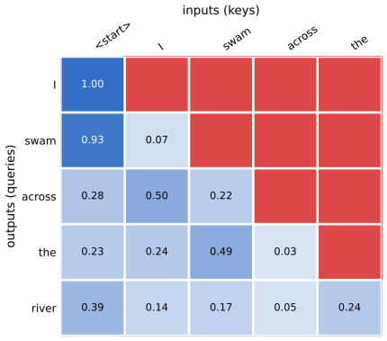
\[ \bY=\Softmax\big[\widetilde\bX\bW^{(p)}\big], \tag{12.33} \]trained with the cross-entropy error (Figure 12.15). Training is self-supervised: each token of a corpus is the target for the tokens before it. Two devices let a whole sequence be processed at once: the input is shifted right by one place with a \(\langle\)start\(\rangle\) token in front, so that input \(n\) is \(x_{n-1}\) and output \(n\) predicts \(x_n\); and every attention layer is masked (causal): the weight of token \(n\) on any later token is set to 0 by putting \(-\infty\) in the score before the softmax, which also renormalises the remaining weights (Figure 12.16). Sequences of different lengths are batched by padding with a \(\langle\)pad\(\rangle\) token that a second, input-dependent mask hides.
Result 12.12 (the causal mask makes training parallel and generation cacheable) pp. 384–386
In a stack of transformer layers in which every attention layer is causally masked and every other operation acts on each position separately, output \(n\) is a function of input tokens \(1,\dots,n\) only. Consequently: (i) one forward pass on \((\langle\)start\(\rangle,x_1,\dots,x_{N-1})\) returns all \(N\) conditionals \(p(x_n\given x_{<n})\), and the summed cross-entropy is the exact negative log-likelihood (12.31) of the sequence; (ii) when a token is appended, the keys and values of all earlier positions are unchanged, so generation can store them (a "key-value cache") and compute only the new row: the \(n\)th token then costs \(O(nD+D^2)\) per layer instead of \(O(n^2D+nD^2)\).
Proof
Induction on the layers. The inputs to layer 1, \(\bx_m+\br_m\), depend on token \(m\) only. Suppose each row \(m\) of the input to layer \(l\) depends on tokens \(\le m\) only. Then \(\bq_n,\bkk_m,\bv_m\) inherit this; with the mask, \(\by_n=\sum_{m\le n}a_{nm}\bv_m\) with \(a_{nm}\) a function of \(\bq_n\) and \(\bkk_1,\dots,\bkk_n\), so \(\by_n\) depends on tokens \(\le n\). The residual sum, the layer norms, the MLP and the output map act row by row and preserve the property. Hence row \(n\) of the output depends on tokens \(\le n\). (i) With the right shift, output \(n\) sees \(\langle\)start\(\rangle,x_1,\dots,x_{n-1}\) and nothing later, so it is a legitimate model of \(p(x_n\given x_{<n})\), and \(\sum_n-\ln p(x_n\given x_{<n})=-\ln p(x_1,\dots,x_N)\) by (12.31). Without the mask, output \(n\) could read \(x_n\) at input \(n+1\) and the network would learn to copy it, useless for generation. (ii) Appending a token changes no row \(m\le n\) of any layer, by the same induction; the new row needs its own projections (\(O(D^2)\)), one row of scores and one weighted sum over the \(n\) cached keys and values (\(O(nD)\)), and the MLP (\(O(D^2)\)). A direct computation verifies on the trained model that the logits at positions 1, 11, 41 and 64 are the same whether computed from the full window or from the prefix alone, and that replacing the last 34 characters changes none of the first 30 outputs (differences below \(10^{-14}\)). (Our browser demo recomputes the whole window at each step instead, because with absolute positions the cache is invalidated once the 64-character window starts to slide.)
The small character transformer used in these notes
Data. Alice's Adventures in Wonderland (Lewis Carroll, 1865; public domain), lower-cased, with curly quotes straightened, dashes turned into hyphens and paragraph breaks kept as newlines: 142 036 characters from a vocabulary of \(K=39\) (26 letters, space, newline and 11 punctuation marks). The first 90% (127 832 characters) is the training text, the last 10% the held-out text.
Model. Decoder-only, pre-norm (12.21), (12.23): character embeddings of dimension \(D=64\) plus the sinusoidal encoding (12.25) with \(L=10\,000\); two layers, each with 4 heads of size 16 and a ReLU MLP of width 256; a final layer norm and the output map (12.33); context of \(N=64\) characters; 105 127 parameters. Embeddings are initialised with standard deviation 0.5 and weight matrices with variance 1/fan-in (the output projections of each sub-layer scaled down by \(\sqrt{2L}\)).
Training. Adam (Section 7.3.3; \(\beta_1=0.9\), \(\beta_2=0.99\)), learning rate \(3\times10^{-3}\) with a 150-step linear warm-up and cosine decay, gradient clipping at norm 1, 3000 steps of 32 random windows of 64 characters (6.1 million predicted characters, about 48 passes over the training text), 2 minutes on one CPU thread. Held-out cross-entropy 1.42 nats per character (perplexity 4.12) against 1.12 on training text: some overfitting, as expected with a corpus this small. A sample at temperature 1 from the prompt "alice was beginning to get very tired of ":
tallice, you know so happen simpleds she felt game with world, "well-i ou!( "i she stairs, the dance of throw faver, as the hanger, led gloves and crembling to do, and man whep as she stairs! it cwle
The weights are exported exactly (float32) and the same forward pass runs in the browser demo, which reproduces the Python logits to \(5\times10^{-15}\) and the sampled text character for character.
12.3.2 Sampling strategies
See also the Viterbi algorithm for hidden Markov models in the companion course, Section 13.2.5.
pp. 386–388 The output of a decoder is a distribution; generation must choose a token (Holtzman et al., 2019). Greedy search takes the most probable token at each step; it is deterministic, but the most probable token at each step need not lie on the most probable sequence (Exercise 12.15), which maximises
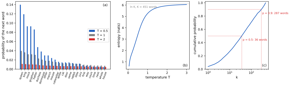
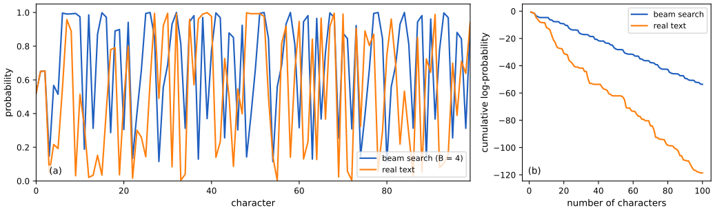
\[ p(y_1,\dots,y_N)=\prod_{n=1}^Np(y_n\given y_1,\dots,y_{n-1}). \tag{12.34} \]There are \(O(K^N)\) sequences, so exhaustive search is impossible; greedy search costs \(O(KN)\). Beam search keeps the \(B\) most probable partial sequences, extends each by its \(B\) best tokens and keeps the best \(B\) of the \(B^2\) candidates, at cost \(O(BKN)\); as products of probabilities shrink with length, scores are usually divided by the length before comparing sequences of different lengths. Greedy and beam search lack diversity and can loop, and human text is less probable under a model than such text (Figure 12.17). Sampling from the full softmax avoids this but sometimes picks a token from the long tail of improbable ones; top-K sampling samples among the \(K\) most probable tokens, nucleus (top-p) sampling among the smallest set of most probable tokens whose probabilities add up to a threshold, and a temperature \(T\) reshapes the softmax (Hinton, Vinyals and Dean, 2015):
\[ y_i=\frac{\exp(a_i/T)}{\sum_j\exp(a_j/T)}. \tag{12.35} \]\(T\to0\) gives greedy selection, \(T=1\) the model, \(T\to\infty\) the uniform distribution. Finally, a model trained on human text but run on its own output can drift away from the training distribution.
Result 12.13 (temperature and truncation) pp. 387–388, (12.35)
Let \(\bq_T=\Softmax(\ba/T)\) for logits \(\ba\in\R^K\). (i) As \(T\to0^+\), \(\bq_T\) tends to the uniform distribution on \(\argmax_ia_i\) (one-hot if the maximum is unique); at \(T=1\) it is \(\Softmax(\ba)\); as \(T\to\infty\) it tends to uniform on all \(K\) tokens. The ranking of the tokens never changes. (ii) The entropy \(H(T)\) of \(\bq_T\) satisfies
\[ \frac{\d H}{\d T}=\frac{\var_{\bq_T}(a)}{T^3}\ge0, \]with equality only when all logits are equal: raising the temperature always spreads the distribution. (iii) Truncation to a set \(S\) of tokens, \(q_i=p_i/p(S)\) for \(i\in S\) and 0 otherwise (top-\(K\) and nucleus sampling at \(T=1\)), has \(\KL(\bq\,\|\,\bp)=-\ln p(S)\); the nucleus \(S_\pi\) is the smallest such set with \(p(S)\ge\pi\), so it is small where the model is confident and large where it is not.
Proof
(i) \(q_{T,i}=e^{(a_i-a_{\max})/T}/\sum_je^{(a_j-a_{\max})/T}\); each exponent tends to 0 for the maximisers and to \(-\infty\) for the others as \(T\to0\), and every exponent tends to 0 as \(T\to\infty\). \(q_{T,i}>q_{T,j}\iff a_i>a_j\) for every \(T>0\). (ii) With \(\beta=1/T\) and \(Z=\sum_je^{\beta a_j}\): \(H=\ln Z-\beta\E_q[a]\). Since \(\d\ln Z/\d\beta=\E_q[a]\) and \(\d\E_q[a]/\d\beta=\var_q(a)\), \(\d H/\d\beta=\E_q[a]-\E_q[a]-\beta\var_q(a)=-\beta\var_q(a)\), and \(\d H/\d T=-\beta\var_q(a)\cdot(-1/T^2)=\var_q(a)/T^3\). (iii) \[\KL(\bq\|\bp)=\sum_{i\in S}\frac{p_i}{p(S)}\ln\frac{p_i/p(S)}{p_i}=-\ln p(S).\] Temperature is a "softer" form of truncation in that it reshapes but never zeroes a probability. On the distribution of the word after "the" in our corpus (451 different words, entropy 5.26 nats), half of the probability needs the 36 commonest words and 90% needs 287 (Figure 12.S6); after "said the" the nucleus for \(\pi=0.5\) has only 6 words. A direct computation confirms (ii) by finite differences on the trained model's logits, (iii) for \(K=5\) and \(\pi=0.5\), and that the demos' inverse-CDF sampler draws from \(\bq\).
Result 12.14 (greedy and beam search are heuristics) pp. 386–387; Exercise 12.15
(i) Greedy search can miss the most probable sequence, already for \(N=2\). (ii) Beam search with width \(B\) returns a sequence at least as probable as greedy search when \(B=1\), but it is not monotone in \(B\): a wider beam can return a less probable sequence. (iii) For a model whose conditionals depend on a bounded number of previous tokens (an n-gram model), the most probable sequence can be found exactly by dynamic programming (the Viterbi algorithm) in \(O(NK^{n})\); for a transformer, whose conditionals depend on the whole prefix, no such shortcut exists.
Proof and examples
(i) See the corrected Exercise 12.15: with \(p(A,A)=0.35\), \(p(A,B)=0.25\), \(p(B,A)=0.4\), \(p(B,B)=0\), greedy picks \(y_1=A\) (\(p(y_1=A)=0.6\)), then \(y_2=A\), probability 0.35, while the best pair \((B,A)\) has 0.4. (ii) On the word bigram model of the sampling demo (60 commonest words of the novel, add-0.5 smoothing), continuing "she" for 4 words: greedy finds "she had to the little" (log-probability \(-6.247\)), beam search with \(B=3\) finds "she was a little of" (\(-6.489\), worse than greedy), and the exact optimum is "she went on the little" (\(-5.708\)). Beam search discards at each step every hypothesis outside the current top \(B\): with \(B=3\), "she went", the start of the optimum, is not among the three best prefixes after one word, and the greedy prefix "she had to" is pruned after three words in favour of prefixes that look better there but continue worse. (iii) For a bigram model, \(\max_{y_1..y_N}\sum_n\ln p(y_n\given y_{n-1})\) satisfies the recursion \(V_n(j)=\max_i[V_{n-1}(i)+\ln p(j\given i)]\), \(O(K^2)\) per step (companion course Section 13.2.5). A transformer's state is the whole prefix, so the number of states grows like \(K^n\). A direct computation confirms (ii) and that Viterbi agrees with brute force over all \(60^3\) continuations of length 3.
12.3.3 Encoder transformers
See also multiclass logistic regression in Section 5.4.4, and in the companion course Section 4.3.4.
pp. 388–390 BERT (Devlin et al., 2018) is pre-trained as an encoder (Figure 12.18): a \(\langle\)class\(\rangle\) token is put in front of every input; a random 15% of the tokens are selected, and the network must predict them from the rest. There is no shift and no causal mask, so each prediction uses context on both sides ("bidirectional"); but only the selected 15% of the positions contribute to the error, and an encoder cannot generate. Since the fine-tuning data contain no \(\langle\)mask\(\rangle\) tokens, of the selected tokens 80% are replaced by \(\langle\)mask\(\rangle\), 10% by a random word and 10% kept, so that 12%, 1.5% and 1.5% of all tokens are masked, randomised and kept-but-predicted. For fine-tuning, a new output layer is attached: for classifying a whole text, a \(D\times K\) matrix and a softmax (or a \(D\times1\) vector and a logistic sigmoid for two classes) on the \(\langle\)class\(\rangle\) output, which is then a multiclass logistic regression on a learned representation; for labelling every token, a shared linear-softmax layer on the other outputs. All parameters are then trained on the labelled task.
Filling the gap 12.8: what the masked-token objective estimates p. 388
Derivation
For a selected set \(M\) of positions, the error is \(-\sum_{n\in M}\ln q(x_n\given\bx_{\setminus M})\), where \(\bx_{\setminus M}\) is the corrupted input. Its expectation over the data is minimised, position by position, by the true conditional \(p(x_n\given\bx_{\setminus M})\) (the cross-entropy \(-\E_p\ln q\) is minimised by \(q=p\), Gibbs' inequality, Section 2.5.5). Unlike (12.31), these conditionals do not multiply to a joint distribution: each is conditioned on a different set, so the sum is a pseudo-likelihood, good for learning representations but not a generative model. Each training sequence of length \(N\) supplies about \(0.15N\) targets, against \(N\) for a decoder under Result 12.12, which is the inefficiency the book mentions.
12.3.4 Sequence-to-sequence transformers
p. 390 For translation, an encoder turns the source sentence into \(\bZ\in\R^{M\times D}\), and a decoder generates the target token by token, conditioned on \(\bZ\) through cross-attention: queries come from the decoder's own sequence, keys and values from \(\bZ\) (Figures 12.19, 12.20), as if a user sent a query to another catalogue. Each decoder layer has masked self-attention, then cross-attention, then the MLP, each with add-and-norm. The model is trained on paired sentences, the source by the encoder and the shifted target by the decoder, with the summed cross-entropy of the target tokens.
Result 12.15 (cross-attention) p. 390, Figure 12.19
With decoder states \(\bX\in\R^{N\times D}\) and encoder outputs \(\bZ\in\R^{M\times D}\), cross-attention is \(\Softmax[\bX\bW^{(q)}(\bZ\bW^{(k)})^\T/\sqrt{D_k}]\,\bZ\bW^{(v)}\): an \(N\times M\) weight matrix, one row per decoder position, and an \(N\times D_v\) output. It is invariant to reordering the rows of \(\bZ\) and equivariant to reordering the rows of \(\bX\). No causal mask is needed in it: every target position may read every source token, while the decoder's self-attention keeps its causal mask, so the model still factorises \(p(\by\given\bx)=\prod_np(y_n\given y_{<n},\bx)\).
Proof
Shapes: \((N\times D_k)(D_k\times M)\) scores, rows normalised over the \(M\) source tokens, times \(M\times D_v\) values. Replacing \(\bZ\) by \(\bP'\bZ\) changes the weights to \(\bA\bP'^\T\) by Result 12.8(i) and the values to \(\bP'\bZ\bW^{(v)}\), so the output \(\bA\bP'^\T\bP'\bZ\bW^{(v)}\) is unchanged: the source enters only through its (encoder) representations, whose order information was added by the encoder's positional encodings. Replacing \(\bX\) by \(\bP\bX\) permutes the rows of the scores and of the output. The factorisation follows from Result 12.12 applied to the decoder, with \(\bZ\) a fixed input. A direct computation confirms the invariance and equivariance.
12.3.5 Large language models
See also the companion course on the best low-rank approximation of a matrix, Section 12.1.2, and transfer learning in Section 6.3.4 of this course.
pp. 390–394 Large language models have up to about \(10^{12}\) parameters. They are possible because parallel hardware suits the transformer, and worthwhile because scaling data and parameters together has improved performance more than architectural ideas (Sutton, 2019; Kaplan et al., 2020); the compute used to train state-of-the-art models has doubled about every 3.4 months since 2012. Self-supervised pre-training on huge corpora, in which every token is a label, replaced supervised training on small curated data. A pre-trained foundation model (Bommasani et al., 2021) is then fine-tuned, cheaply, for each downstream task, by adding or replacing output layers and adapting the main weights a little or not at all.
Result 12.16 (low-rank adaptation) pp. 392–393, (12.36), Figure 12.21
LoRA (Hu et al., 2021) freezes a pre-trained \(\bW_0\in\R^{D\times D}\) and trains \(\bA\in\R^{D\times R}\), \(\bB\in\R^{R\times D}\), the layer computing \(\bX\bW_0+\bX\bA\bB\). Then (i) the update \(\bA\bB\) has rank at most \(R\) and \(2RD\) parameters instead of \(D^2\) (a factor \(D/2R\) fewer); (ii) after training, the merged matrix
\[ \widehat\bW=\bW_0+\bA\bB \tag{12.36} \]gives the same outputs, \(\bX\widehat\bW=\bX\bW_0+\bX\bA\bB\), with no extra cost at inference; (iii) the set of updates it can represent is exactly the matrices of rank \(\le R\), and among them the one closest in Frobenius norm to a desired full update \(\Delta\) is its truncated singular value decomposition.
Proof
(i) \(\rank(\bA\bB)\le\min(\rank\bA,\rank\bB)\le R\); counting entries gives \(DR+RD\). (ii) Distributivity of the matrix product. (iii) Every matrix of rank \(\le R\) factors as \(\bA\bB\) (take its SVD and split the singular values), and the best rank-\(R\) approximation in Frobenius norm is the truncated SVD (Eckart–Young; see the minimum-error formulation of PCA in the companion course, Section 12.1.2). With \(D=4096\) and \(R=8\) the factor is 256 for one matrix; the factor of 10 000 quoted in the book refers to a whole model in which most matrices are frozen. In practice \(\bB\) is initialised to zero, so that fine-tuning starts exactly at the pre-trained model. A direct computation confirms (i) and (ii).
pp. 393–394 Large enough models need little fine-tuning: given "English: the cat sat on the mat. French:" a language model continues with a translation it was never explicitly trained to produce. Models are further tuned with human feedback (reinforcement learning from human feedback, Christiano et al., 2017) to make conversational systems. The input is a prompt; its design (prompt engineering, Liu et al., 2021) and a prepended prefix prompt steer the output, and examples placed in the prompt let the model solve a new task without changing its parameters (few-shot learning).
12.4 Multimodal transformers
pp. 394–395 Transformers make few assumptions about their input, unlike convolutional networks with their built-in locality and translation equivariance (Chapter 10), and are now the state of the art for text, images, video, point clouds and audio, for both discrimination and generation. The layer itself has hardly changed; the innovations are in how inputs are turned into tokens and outputs decoded. A single architecture also makes multimodal models simple: if every input can be tokenised and every output token decoded, a transformer can probably be used.
12.4.1 Vision transformers
See also the companion course, convolutional networks and weight sharing, Section 5.5.6.
pp. 395–396 A vision transformer (ViT; Dosovitskiy et al., 2020) is a transformer encoder for images. Pixels as tokens would make the \(N^2\) cost prohibitive, so an image \(\bx\in\R^{H\times W\times C}\) is cut into non-overlapping \(P\times P\) patches (\(P=16\) is common), each flattened into a vector of length \(P^2C\): \(\bx_p\in\R^{N\times(P^2C)}\) with \(N=HW/P^2\). A linear map embeds each patch, a learnable \(\langle\)class\(\rangle\) token is added, and the class is read from its output by a linear-softmax layer (Figure 12.22). Alternatively a small CNN can make the tokens: a ResNet-18 trunk reduces height and width by 8, giving 64 times fewer tokens than pixels. Positions are usually learned, which is safe because the number of patches is fixed. The only two-dimensional bias of a ViT is the patching; it must learn the geometry of images from data, so it needs more data than a CNN but can end up more accurate, an instance of the trade-off between inductive bias and data (Sutton, 2019).
Filling the gap 12.9: patch embedding is a strided convolution p. 395
Derivation
Let \(\bE\in\R^{P^2C\times D}\) embed a flattened patch. Token \((i,j)\) (patch row \(i\), column \(j\)) is \[\sum_{u,v,c}x_{iP+u,\,jP+v,\,c}\,E_{(u,v,c),d}\] for output channel \(d\), which is exactly a convolution of the image with \(D\) filters of size \(P\times P\times C\) (filter \(d\) holding column \(d\) of \(\bE\)) evaluated with stride \(P\), so that the receptive fields tile the image without overlap. So a ViT starts with one convolutional layer with no nonlinearity, and everything after it is permutation-equivariant across patches except for the learned positions. A direct computation confirms the identity against PyTorch's convolution for a \(28\times28\times3\) image with \(P=7\) (16 patches of length 147).
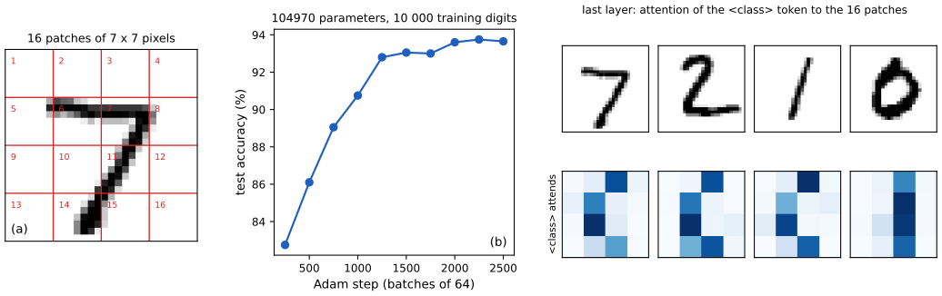
12.4.2 Generative image transformers
See also the companion course: the lecture on autoregressive models and its pixel-by-pixel generation demo; K-means and vector quantisation in Section 9.1 and 9.1.1.
pp. 396–399 Images have no natural order, but any distribution factorises along any chosen ordering (Section 11.1.2):
\[ p(\bx_1,\dots,\bx_N)=\prod_{n=1}^Np(\bx_n\given\bx_1,\dots,\bx_{n-1}), \tag{12.37} \]with no restriction on the conditionals. With pixels in raster-scan order (Figure 12.23), an image is generated one pixel at a time (Figure 12.24), as did PixelCNN and PixelRNN (Oord et al., 2016; Oord, Kalchbrenner and Kavukcuoglu, 2016) with masked convolutions before transformers.
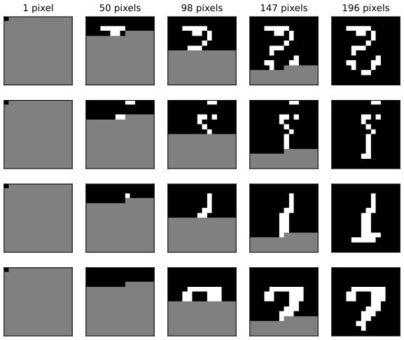
For generation, discrete pixel values work much better than continuous ones: a Gaussian conditional fitted by maximum likelihood (a sum-of-squares error) averages the possibilities, while a categorical distribution can say "black or white" (Filling the gap 12.10). But 8-bit RGB pixels have \(2^{24}\approx1.7\times10^7\) values, too many for a softmax. Vector quantisation compresses them: with a codebook \(\mathcal{C}=\{\bc_1,\dots,\bc_K\}\) of vectors of the same dimension, each data vector is replaced by its nearest code vector,
\[ \bx_n\to\argmin_{\bc_k\in\mathcal{C}}\|\bx_n-\bc_k\|^2, \tag{12.38} \]and so by a one-hot vector of length \(K\), which trades accuracy (large \(K\)) against compression (small \(K\)). ImageGPT (Chen, Radford et al., 2020) used K-means clusters of colours as tokens, trained like a language model. Pixels as tokens are expensive, so patches are better, but the number of possible patches is exponential in their size: binary \(16\times16\) patches already have \(2^{256}\approx1.2\times10^{77}\) values. Codebooks for patches are learned by K-means or by networks (Oord, Vinyals and Kavukcuoglu, 2017; Esser, Rombach and Ommer, 2020; Yu et al., 2021); videos are sequences of such tokens.
Filling the gap 12.10: why a Gaussian conditional draws grey, and how the codebook is trained through a non-differentiable step pp. 397–399
Derivation
Grey. Suppose that, given the pixels so far, the next pixel is black (0) or white (1) with probability \(\frac12\) each. A Gaussian \(\N(x\given\mu,\sigma^2)\) fitted by maximum likelihood has \(\mu=\E[x]=\frac12\) and \(\sigma^2=\var[x]=\frac14\): its most probable value is grey, a value that never occurs, and samples are spread over \([-0.5,1.5]\). More generally, minimising the sum-of-squares error gives the conditional mean (Section 4.2), which averages the modes. A categorical distribution over \(\{0,1\}\) represents \((\frac12,\frac12)\) exactly; with a softmax over \(K\) values any multimodal conditional is representable. That is why our pixel model of Figure 12.24 uses two tokens.
K-means is vector quantisation with a learned codebook. For fixed codes, (12.38) is the assignment step of K-means; for fixed assignments, the squared error is minimised by putting each \(\bc_k\) at the mean of its assigned vectors; alternating the two never increases the distortion (companion course, Section 9.1; its Section 9.1.1 compresses an image this way). A direct computation confirms that (12.38) returns the nearest code.
Straight-through gradients. When the codebook sits inside a network (an encoder \(\bz=g(\bx)\), quantisation \(\bz_q=\bc_{k(\bz)}\), a decoder), \(\bz_q\) is piecewise constant in \(\bz\), so its derivative is 0 almost everywhere and no gradient reaches the encoder. The straight-through estimator (Bengio, Léonard and Courville, 2013) uses \(\bz_q\) in the forward pass but treats \(\partial\bz_q/\partial\bz\) as the identity in the backward pass, i.e. it passes \(\partial E/\partial\bz_q\) to \(\bz\) unchanged. This is a biased approximation, accurate when \(\bz_q\) is close to \(\bz\); it is implemented as \(\bz_q=\bz+\operatorname{stopgrad}(\bc_{k(\bz)}-\bz)\).
12.4.3 Audio data
pp. 399–400 Sound is stored as samples of air pressure, but networks work better on a mel spectrogram (Figure 12.25).
Definition 12.3 (mel spectrogram) p. 399
Cut the waveform into overlapping frames (here 512 samples, every 96 samples), multiply each by a window (Hann) and take its discrete Fourier transform \(X_t(f)\); the power \(|X_t(f)|^2\) at frame \(t\) and frequency \(f\) is the spectrogram. Then map frequency to the mel scale, \(m(f)=2595\log_{10}(1+f/700)\), roughly linear below 1 kHz and logarithmic above, chosen so that equal steps sound equally far apart; sum the power with \(M\) triangular filters whose centres are equally spaced in mel (each rising from 0 to 1 and back over three consecutive centres); and take \(10\log_{10}\) of the result (decibels). The result is an \(M\times(\text{number of frames})\) image: rows are mel bands, columns time.
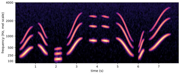
For audio classification (AudioSet, Gemmeke et al., 2017, with classes such as "car" and "laughter"), CNNs on spectrograms used to be the state of the art; the audio spectrogram transformer (Gong, Chung and Glass, 2021) instead treats the spectrogram as an image, splits it into (possibly overlapping) patches flattened to length 256, adds positions and a \(\langle\)class\(\rangle\) token, and uses the same encoder as for text and images, trained end to end with the cross-entropy. Unlike a CNN it relates distant parts of the recording directly.
12.4.4 Text-to-speech
pp. 400–402 Regression from text to spectrograms needs a lot of data per speaker, needs long contexts to sound fluent, and averages over the many correct ways to say a sentence. Treated instead as conditional language modelling, speech becomes a sequence of discrete tokens from a learned codebook (vector quantisation, as above). Vall-E (Wang et al., 2023) feeds a transformer with the text tokens followed by a few seconds of speech tokens from the target speaker (the acoustic prompt) and trains it to produce the speech tokens of the text (Figure 12.26); trained on many speakers, it reads new text in the voice of a new speaker from a three-second sample, and a learned decoder turns the sampled tokens back into a waveform.
12.4.5 Vision and language transformers
pp. 402–403 Text, images and audio can all be tokenised, so one model can take and produce any mixture. Large paired data sets such as LAION-400M (Schuhmann et al., 2021) made text-to-image generation and captioning practical. Text-to-image generation is conditional image generation, a sequence-to-sequence problem with image tokens as the target, solved by an encoder-decoder (Figure 12.20) in Parti (Yu et al., 2022), which improved steadily up to 20 billion parameters. Other work adapts pre-trained language models to accept continuous image features (Alayrac et al., 2022; Li et al., 2022), which cannot easily output images or add new modalities. The simplest general approach uses one vocabulary, the union of text tokens and image codebook entries, and models everything as one sequence: CM3 (Aghajanyan et al., 2022) and CM3Leon (Yu et al., 2023) are trained on web documents mixing text and images, and perform captioning, text-to-image generation, image editing and text completion with one model (Figure 12.27, not reproduced: it shows outputs of that large model).
Corrections to the chapter (first printing)
- p. 363 and Exercise 12.3: orthogonal inputs are not mapped to themselves by (12.2) with (12.5): \[a_{nn}=e^{\|\bx_n\|^2}/(e^{\|\bx_n\|^2}+N-1)<1,\] so \(\by_n\ne\bx_n\); the statement holds only approximately, when \(\|\bx_n\|^2\gg\ln N\) (Result 12.1; for \(N=11\) and unit norms \(a_{nn}=0.214\), checked).
- Exercise 12.5, (12.42): \(\bH_h\bX\bW^{(h)}\) with \(\bH_h\) from (12.15) is dimensionally undefined (\(N\times D_v\) times \(N\times D\)); the factor must be the \(N\times N\) attention-weight matrix \(\bA_h\) (Result 12.5, checked).
- Exercise 12.15: the table's four probabilities sum to 0.75, not 1, and its largest entry is \(p(y_1=B,y_2=A)=0.4\), not \((B,B)\) as the text says; after normalisation greedy search does find the most probable pair, so the table does not illustrate the point. A consistent table is given in the solution (checked).
- Algorithm 12.1: \(\bV\in\R^{N\times D}\) should be \(\R^{N\times D_v}\). Algorithm 12.2: \(\bW^{(q)}_h,\bW^{(k)}_h\in\R^{D\times D}\) should be \(\R^{D\times D_k}\); \(\Concat[\bH_1,\dots,\bH_N]\) should end with \(\bH_H\); the output \(\{\by_1,\dots,\bx_N\}\) should end with \(\by_N\).
- p. 369: the outputs of an attention layer lie in the image of the span of the inputs under \(\bW^{(v)}_h\bW^{(o)}_h\) (summed over heads), not in that span itself, unless these maps are the identity (Filling the gap 12.3).
- Figure 12.14: the decoder's third input reads "gelukigg"; it should be "gelukkig", the word output at the previous step.
Exercises
All 16 exercises of Chapter 12 (Bishop and Bishop, 2024, pp. 403–406), restated in my own words, with complete solutions (hidden). Stars give the book's difficulty. The official solutions manual covers Chapters 2 to 10 only, so these solutions are my own; the numerical ones were confirmed by direct computation.
Exercise 12.1 (★★). Coefficients \(a_{nm}\), \(m=1,\dots,N\), satisfy \(a_{nm}\ge0\) (12.39) and \(\sum_ma_{nm}=1\) (12.40). Using a Lagrange multiplier, show that
\[ a_{nm}\le1\quad\text{for all }m. \tag{12.41} \]Solution
Directly: \(a_{nk}=1-\sum_{m\ne k}a_{nm}\le1\) because the subtracted terms are non-negative. With multipliers, as the exercise asks: maximise \(a_{nk}\) subject to the constraints. The Lagrangian (with Karush–Kuhn–Tucker multipliers \(\mu_m\ge0\) for the inequalities) is \(L=a_{nk}+\lambda(1-\sum_ma_{nm})+\sum_m\mu_ma_{nm}\). Stationarity gives \(\delta_{mk}-\lambda+\mu_m=0\), so \(\mu_m=\lambda\) for \(m\ne k\) and \(\mu_k=\lambda-1\). Since \(\mu_k\ge0\), \(\lambda\ge1>0\), hence \(\mu_m>0\) for \(m\ne k\), and complementary slackness \(\mu_ma_{nm}=0\) forces \(a_{nm}=0\) for \(m\ne k\); then (12.40) gives \(a_{nk}=1\). The maximum of any coefficient is therefore 1, which is (12.41). (Lagrange multipliers: companion course toolkit.)
Exercise 12.2 (★). Show that the softmax weights (12.5) satisfy (12.3) and (12.4) for any input vectors.
Solution
Each numerator \(\exp(\bx_n^\T\bx_m)\) is strictly positive for any real exponent, so \(a_{nm}>0\), stronger than (12.3). The denominator is the sum of the numerators over \(m\), so \(\sum_ma_{nm}=1\), which is (12.4). The same holds for any real scores, scaled, masked (a score \(-\infty\) gives weight 0) or not. A direct computation confirms it for scores of size 100, where a naive implementation would overflow; subtracting the row maximum first avoids that without changing the result.
Exercise 12.3 (★). Show that if the inputs are orthogonal, \(\bx_n^\T\bx_m=0\) for \(n\ne m\), then (12.2) with (12.5) gives \(\by_n=\bx_n\).
Solution
The statement is false (Result 12.1). The off-diagonal weights are \(a_{nm}=1/(e^{\|\bx_n\|^2}+N-1)>0\), and as the inputs are linearly independent, \(\by_n=\sum_ma_{nm}\bx_m\) equals \(\bx_n\) only if every \(a_{nm}\), \(m\ne n\), is 0. What is true: \[\|\by_n-\bx_n\|^2=N(N-1)s^2/(e^{s^2}+N-1)^2\] for inputs of equal norm \(s\), which tends to 0 when \(s^2-\ln N\to\infty\); so \(\by_n\approx\bx_n\) for orthogonal inputs of large norm. Example: \(N=11\), \(s=1\) gives \(a_{nn}=0.214\); \(s=3\) gives 0.9988 (checked). Demo preset 3 shows this.
Exercise 12.4 (★). For independent \(\ba,\bb\sim\N(\bzero,\bI_D)\), show that \(\E[(\ba^\T\bb)^2]=D\).
Solution
\[\E[(\ba^\T\bb)^2]=\sum_{i,j}\E[a_ia_j]\E[b_ib_j]=\sum_{i,j}\delta_{ij}^2=D,\] using independence of \(\ba\) and \(\bb\) and \(\E[a_ia_j]=\delta_{ij}\). Only zero means, unit variances and uncorrelated components are used, not Gaussianity (Result 12.4). Monte Carlo gives 15.9 for \(D=16\), 254.4 for \(D=256\), and variance \(D\) for random-sign entries.
Exercise 12.5 (★★★). Show that multi-head attention (12.19) can be written as a sum over heads,
\[ \bY=\sum_{h=1}^H\bH_h\bX\bW^{(h)}\quad\text{(as printed)}, \tag{12.42} \] \[ \bW^{(h)}=\bW^{(v)}_h\bW^{(o)}_h, \tag{12.43} \]with \(\bW^{(o)}_h\in\R^{D_v\times D}\) the row blocks of \(\bW^{(o)}\); explain why, with \(D_v<D\), the matrices \(\bW^{(h)}\) are rank-deficient, so that replacing them by unrestricted matrices would change the model.
Solution
See Result 12.5. Block multiplication gives \(\bY=\sum_h\bH_h\bW^{(o)}_h\), and \(\bH_h=\bA_h\bX\bW^{(v)}_h\), so \(\bY=\sum_h\bA_h\bX\bW^{(v)}_h\bW^{(o)}_h=\sum_h\bA_h\bX\bW^{(h)}\). Correction: in (12.42) the factor must be the \(N\times N\) weight matrix \(\bA_h=\Softmax[\bQ_h\bK_h^\T/\sqrt{D_k}]\); with \(\bH_h\) from (12.15) (an \(N\times D_v\) matrix) the product \(\bH_h\bX\) is undefined. Rank: \(\bW^{(h)}\) is \(D\times D\) but factors through \(\R^{D_v}\), so \(\rank\bW^{(h)}\le D_v=D/H<D\). Unrestricted \(D\times D\) matrices would include all these and more (and cost \(HD^2\) parameters instead of \(2D^2\)), so the models are not equivalent. Checked numerically, including the ranks.
Exercise 12.6 (★★). Write self-attention (12.14) as a matrix acting on the concatenated input vectors, compare with a fully connected layer (\(O(N^2D^2)\) parameters), show that attention is a sparse, weight-shared version, and sketch which blocks are shared and which are zero.
Solution
Stack the tokens into \(\vecop(\bX)=(\bx_1;\dots;\bx_N)\in\R^{ND}\). One head computes \(\by_n=\sum_ma_{nm}\bW^{(v)\T}\bx_m\) (taking \(D_v=D\)), so \(\vecop(\bY)=\bM\vecop(\bX)\) with \(\bM=\bA\otimes\bW^{(v)\T}\): an \(N\times N\) grid of \(D\times D\) blocks, block \((n,m)\) equal to \(a_{nm}\bW^{(v)\T}\) (Result 12.7, Figure 12.S8). A fully connected layer would have \(N^2\) independent blocks, \(N^2D^2\) parameters. In attention every block is the same matrix up to a scalar, so there are only the \(D^2\) entries of \(\bW^{(v)}\) (plus \(2DD_k\) in \(\bW^{(q)},\bW^{(k)}\), which produce the scalars); the matrix is not fixed but recomputed for each input, since the \(a_{nm}\) depend on \(\bX\). With the causal mask all blocks above the diagonal are zero. The position-wise MLP layer is the opposite extreme: \(\bI_N\otimes\bW^\T\), identical blocks on the diagonal and zeros elsewhere. With \(H\) heads, \(\bM=\sum_h\bA_h\otimes\bW^{(h)\T}\), a sum of \(H\) such structured matrices. The Kronecker identity is checked exactly.
Exercise 12.7 (★). Show that without positional encoding, multi-head attention (12.19) is equivariant to reordering the input sequence.
Solution
For a permutation matrix \(\bP\): queries, keys and values become \(\bP\bQ_h,\bP\bK_h,\bP\bV_h\); the scores \(\bP\bQ_h\bK_h^\T\bP^\T\); since a row-wise softmax commutes with permuting rows and with permuting the entries of every row in the same way, the weights become \(\bP\bA_h\bP^\T\); the head output \(\bP\bA_h\bP^\T\bP\bV_h=\bP\bH_h\); concatenation and \(\bW^{(o)}\) act on columns, so \(\bY(\bP\bX)=\bP\bY(\bX)\). Full proof, including the whole layer and what breaks equivariance, in Result 12.8; checked to \(10^{-12}\).
Exercise 12.8 (★★★). Let \(\ba,\bb\) be random unit vectors in \(\R^D\) with a rotation-invariant distribution. Using an orthonormal basis, show that for large \(D\) the cosine of the angle between them is close to zero.
Solution
Expand \(\ba=\sum_i\alpha_i\bu_i\) in an orthonormal basis \(\{\bu_i\}\) chosen, after drawing \(\bb\), with \(\bu_1=\bb\); then \(\cos\theta=\ba^\T\bb=\alpha_1\). Rotation invariance means the distribution of \((\alpha_1,\dots,\alpha_D)\) does not depend on which basis is used, so all \(\alpha_i\) have the same distribution; with \(\sum_i\alpha_i^2=\|\ba\|^2=1\) this gives \(\E[\alpha_1^2]=1/D\). Also \(\E[\alpha_1]=0\) (the distribution is symmetric under \(\ba\to-\ba\)). So \(\E[\cos\theta]=0\), \(\var[\cos\theta]=1/D\), and by Chebyshev \(P(|\cos\theta|\ge t)\le1/(Dt^2)\to0\) for every fixed \(t>0\): random directions are nearly orthogonal in high dimension. Monte Carlo for \(D=512\): \(\E[\cos^2\theta]=0.00196\) against \(1/512=0.00195\) (Filling the gap 12.5).
Exercise 12.9 (★★). A token \(\bx\) is concatenated with a position vector \(\be\). Show that multiplying the concatenation by a matrix gives the sum of a linearly transformed token and a linearly transformed position.
Solution
Partition the matrix by columns, \(\bW=[\bW_x\ \bW_e]\), conformably with \((\bx;\be)\). Block multiplication gives \(\bW(\bx;\be)=\bW_x\bx+\bW_e\be\). So every linear map of the concatenation is a sum of separate linear maps of the parts, which is the additive scheme (12.24) applied after the maps; conversely, \(\bx+\be=[\bI\ \bI](\bx;\be)\). Since a transformer uses its inputs only through linear maps at first, the two schemes are equivalent in what the first layer can compute, apart from the dimension (Filling the gap 12.5; checked).
Exercise 12.10 (★★). Using the addition formulas
\[ \cos(A+B)=\cos A\cos B-\sin A\sin B, \tag{12.44} \] \[ \sin(A+B)=\cos A\sin B+\sin A\cos B, \tag{12.45} \]show that for the encoding (12.25) and any fixed offset \(k\), \(\br_{n+k}\) is a linear combination of the components of \(\br_n\) with coefficients that depend on \(k\) but not on \(n\); and that this fails if only sines are used.
Solution
For each frequency \(\omega_j\), with \(A=\omega_jn\), \(B=\omega_jk\): \[\sin\omega_j(n+k)=\cos\omega_jk\,\sin\omega_jn+\sin\omega_jk\,\cos\omega_jn\] and \[\cos\omega_j(n+k)=\cos\omega_jk\,\cos\omega_jn-\sin\omega_jk\,\sin\omega_jn.\] So \(\br_{n+k}=\bM(k)\br_n\) with the block-diagonal rotation matrix of Result 12.9, which depends on \(k\) only. The cosine of each frequency is needed because \(\sin\omega_j(n+k)\) involves \(\cos\omega_jn\). Sines only: if \(\sin\omega_j(n+k)=\sum_iM_{ji}\sin\omega_in\) held for all \(n\), then at \(n=0\) the right side is 0, so \(\sin\omega_jk=0\) for every \(j\), which fails for general \(k\); the argument without position 0 is in Result 12.9(5). Numerically, the best least-squares matrix for sines only leaves a 40% residual, while the rotation is exact to \(10^{-14}\).
Exercise 12.11 (★). For the bag-of-words model (12.28) with one shared probability table, show that the maximum-likelihood table is the relative frequency of each word in the training set.
Solution
With counts \(n_k\) and \(N=\sum_kn_k\), the log-likelihood is \(\sum_kn_k\ln\pi_k\); maximising subject to \(\sum_k\pi_k=1\) with a Lagrange multiplier gives \(n_k/\pi_k=\lambda\), so \(\pi_k=n_k/N\) (Result 12.11(i); concavity makes it the global maximum). Equivalently, \(\sum_kn_k\ln\pi_k=-N[\KL(\widehat{\bp}\|\boldsymbol\pi)+H(\widehat{\bp})]\) with \(\widehat p_k=n_k/N\), maximised by \(\boldsymbol\pi=\widehat{\bp}\). (Companion course Section 2.2; checked against perturbed tables on our corpus.)
Exercise 12.12 (★). If the conditionals of (12.31) are general tables, show that their size grows exponentially with \(n\).
Solution
\(p(x_n\given x_1,\dots,x_{n-1})\) needs one distribution over \(K\) values for each of the \(K^{n-1}\) possible contexts: \(K^n\) entries, \(K^{n-1}(K-1)\) of them free. This grows like \(K^n\). Over the whole sequence the free parameters add up to \(K^N-1\), the same as an unrestricted joint distribution (Result 12.11(iv)). For \(K=39\) characters, \(n=4\) already needs 2 254 122 free entries, and a word vocabulary of \(K=50\,000\) with \(n=3\) needs \(1.25\times10^{14}\).
Exercise 12.13 (★). n-gram conditionals are often computed from L-gram and \((L-1)\)-gram tables by the product rule,
\[ p(x_n\given x_{n-L+1},\dots,x_{n-1})=\frac{p_L(x_{n-L+1},\dots,x_n)}{p_{L-1}(x_{n-L+1},\dots,x_{n-1})}. \tag{12.46} \]Explain why this is more convenient than storing the conditional, and show that to get correct probabilities the final token of each sequence must be left out when estimating \(p_{L-1}\).
Solution
Convenience. Counting L-grams and \((L-1)\)-grams is one pass of counting with no normalisation per context; the joint tables are what one smooths, prunes and backs off with (a lower-order table is needed anyway when an L-gram is unseen), and lower orders are available for free; the conditional is a ratio computed on demand. The final token. The conditional must sum to 1 over \(x_n\): \(\sum_xp_L(c,x)=p_{L-1}(c)\) for every context \(c\). The counts in the numerators come from the L-grams, each of which starts with an \((L-1)\)-gram that is followed by a token; an \((L-1)\)-gram at the very end of a sequence has no successor and appears in no L-gram. So \(p_{L-1}\) must be estimated from the \((L-1)\)-grams that are followed by something, i.e. leaving out the one that ends each sequence; otherwise the denominator is too large for the contexts that end a sequence and their conditionals sum to less than 1. Example: in "abracadabra" with \(L=3\), the bigram "ra" occurs twice but is followed by a token only once; counting both gives \(p(c\given\text{ra})\) summing to \(\frac12\). A direct computation confirms this, and that the corrected ratios sum to 1 for every context.
Exercise 12.14 (★★). Write pseudo-code for inference in a trained RNN of the form of Figure 12.13.
Solution
Let \(f_\bw\) map \((\bz_{\rm prev},\bx)\) to \((\bz,\by)\), where \(\by\) is a softmax over tokens. Scoring or labelling a given sequence:
z = z0                       # e.g. the zero vector
for n = 1, ..., N:
    z, y[n] = f_w(z, x[n])   # same weights at every step
return y[1..N]
Generation (the decoder of Figure 12.14, or a language model):
z = z0
for n = 1, ..., N_in:        # absorb the input (prompt or source sentence)
    z, _ = f_w(z, x[n])      # outputs ignored
tok = <start>; out = []
repeat:
    z, p = f_w(z, embed(tok))
    tok = choose(p)          # argmax, or a sample (Section 12.3.2)
    if tok == <stop> or len(out) == max_len: break
    out.append(tok)          # fed back as the next input
return out
Each step costs one evaluation of \(f_\bw\), so generation is \(O(N)\) evaluations, but they are strictly sequential, unlike the parallel training of a masked transformer (Result 12.12).
Exercise 12.15 (★★). Two tokens \(y_1,y_2\in\{A,B\}\) have the joint distribution in the table below, and the most probable sequence is said to be \((B,B)\) with probability 0.4. Find \(p(y_1)\) and \(p(y_2\given y_1)\), show that maximising \(p(y_1)\) and then \(p(y_2\given y_1^\star)\) gives a different sequence, and find its probability.
\(y_1=A\) \(y_1=B\) \(y_2=A\) 0.0 0.4 \(y_2=B\) 0.1 0.25 Solution
The printed table is inconsistent. Its entries sum to 0.75, not 1, and its largest entry is \(p(y_1=B,y_2=A)=0.4\), not \((B,B)\). Normalising by 0.75: \(p(y_1=A)=0.1/0.75=0.133\), \(p(y_1=B)=0.867\); \(p(y_2=A\given y_1=B)=0.4/0.65=0.615\). Greedy picks \(y_1=B\), then \(y_2=A\): the pair \((B,A)\), which is the most probable pair (probability \(0.4/0.75=0.533\)), so the table does not show what the exercise intends (checked).
A corrected version that does: \(p(A,A)=0.35\), \(p(A,B)=0.25\), \(p(B,A)=0.4\), \(p(B,B)=0\) (sum 1; best pair \((B,A)\), probability 0.4). Then \(p(y_1=A)=0.6\), \(p(y_1=B)=0.4\); \(p(y_2=A\given A)=0.35/0.6=0.583\), \(p(y_2=B\given A)=0.417\), \(p(y_2=A\given B)=1\), \(p(y_2=B\given B)=0\). Greedy: \(y_1^\star=A\) (0.6 > 0.4), then \(y_2^\star=A\) (0.583): the sequence \((A,A)\), with probability \(0.6\times0.583=0.35<0.4\). The first step's choice is locally best but leads to a worse sequence, because the probability of \(y_1=B\) is concentrated on a single continuation (Result 12.14; checked).
Exercise 12.16 (★). BERT-Large has inputs of up to 512 tokens of dimension \(D=1024\) from a vocabulary of 30 000, 24 layers each with 16 heads of size \(D_q=D_k=D_v=64\), and position-wise MLPs with 4096 hidden units. Show that it has about 340 million parameters.
Solution
Per layer (Result 12.6): attention \(4\cdot1024^2+4\cdot1024=4\,198\,400\) (since \(16\times64=1024\)); MLP \[2\cdot1024\cdot4096+4096+1024=8\,393\,728;\] two layer norms \(4096\): total \(12\,596\,224\), times 24 layers \(=302\,309\,376\). Embeddings: \(30\,000\times1024=30\,720\,000\) token vectors, \(512\times1024=524\,288\) positions, 2048 for the two segment vectors and 2048 for the embedding layer norm: \(31\,248\,384\). The output "pooler" on the \(\langle\)class\(\rangle\) token adds \(1\,049\,600\). Total \(334\,607\,360\approx335\) million, about 340 million; the weights in the layers dominate (90%), and of those two thirds are in the MLPs. (The masked-token output layer reuses the embedding matrix, adding only \(D^2+3D\) for a transform and \(K\) biases.)
Demonstrations
Three interactive pages, each linked above where its topic arises. They run in the browser and reproduce the Python code number for number (attention weights and sampling distributions to \(2\times10^{-15}\), the trained model's logits to \(5\times10^{-15}\), and the sampled, greedy and beam-search texts character for character).
- Attention explorer: the attention matrix of a sentence with identity, shared or independent query/key/value maps, any dimension, with or without the \(1/\sqrt{D}\) scaling, a temperature, the causal mask, sinusoidal encodings and a permutation test. Presets: 1 scaled attention, 2 saturation without scaling, 3 orthogonal inputs (Exercise 12.3), 4 causal mask, 5 equivariance, 6 positions break it, 7 relative offsets.
- Sampling strategies: temperature, top-k and nucleus sampling on next-word distributions counted in the novel, with entropies, KL divergences and seeded draws; greedy, beam and exact (Viterbi) search on a word bigram model. Presets: 1 pure sampling, 2 T = 0.5, 3 T = 2, 4 top-k, 5 nucleus, 6 greedy, beam and exact.
- A character transformer in the browser: the model of Section 12.3.1 generating text from any prompt by sampling, greedy or beam search, with the probability of each character, the next-character distribution and the attention of every head. Presets: 1 T = 1, 2 greedy loops, 3 T = 0.5, 4 T = 1.6, 5 nucleus, 6 beam search against real text.
References
- Bishop, C. M. and Bishop, H. (2024). Deep Learning: Foundations and Concepts. Springer, Cham. Chapter 12, pp. 357–406. doi:10.1007/978-3-031-45468-4. Book website: www.bishopbook.com.
- Ba, J. L., Kiros, J. R. and Hinton, G. E. (2016). Layer normalization. arXiv:1607.06450.
- Bahdanau, D., Cho, K. and Bengio, Y. (2014). Neural machine translation by jointly learning to align and translate. arXiv:1409.0473.
- Bengio, Y., Léonard, N. and Courville, A. (2013). Estimating or propagating gradients through stochastic neurons for conditional computation. arXiv:1308.3432.
- Brown, T. B. et al. (2020). Language models are few-shot learners. In Advances in Neural Information Processing Systems 33.
- Carroll, L. (1865). Alice's Adventures in Wonderland. Macmillan, London. Public domain; the text used for the models of these notes.
- Chen, M., Radford, A. et al. (2020). Generative pretraining from pixels. In Proceedings of the 37th International Conference on Machine Learning.
- Devlin, J., Chang, M.-W., Lee, K. and Toutanova, K. (2018). BERT: pre-training of deep bidirectional transformers for language understanding. arXiv:1810.04805.
- Dosovitskiy, A. et al. (2020). An image is worth 16x16 words: transformers for image recognition at scale. arXiv:2010.11929.
- Gong, Y., Chung, Y.-A. and Glass, J. (2021). AST: audio spectrogram transformer. In Proceedings of Interspeech 2021.
- Hinton, G., Vinyals, O. and Dean, J. (2015). Distilling the knowledge in a neural network. arXiv:1503.02531.
- Hochreiter, S. and Schmidhuber, J. (1997). Long short-term memory. Neural Computation, 9(8), 1735–1780.
- Holtzman, A., Buys, J., Du, L., Forbes, M. and Choi, Y. (2019). The curious case of neural text degeneration. arXiv:1904.09751.
- Hu, E. J. et al. (2021). LoRA: low-rank adaptation of large language models. arXiv:2106.09685.
- Kaplan, J. et al. (2020). Scaling laws for neural language models. arXiv:2001.08361.
- Levy, O. and Goldberg, Y. (2014). Neural word embedding as implicit matrix factorization. In Advances in Neural Information Processing Systems 27.
- Mikolov, T., Chen, K., Corrado, G. and Dean, J. (2013). Efficient estimation of word representations in vector space. arXiv:1301.3781.
- Oord, A. van den, Vinyals, O. and Kavukcuoglu, K. (2017). Neural discrete representation learning. In Advances in Neural Information Processing Systems 30.
- Radford, A., Wu, J., Child, R., Luan, D., Amodei, D. and Sutskever, I. (2019). Language models are unsupervised multitask learners. Technical report, OpenAI.
- Sennrich, R., Haddow, B. and Birch, A. (2015). Neural machine translation of rare words with subword units. arXiv:1508.07909.
- Su, J., Lu, Y., Pan, S., Murtadha, A., Wen, B. and Liu, Y. (2021). RoFormer: enhanced transformer with rotary position embedding. arXiv:2104.09864.
- Vaswani, A., Shazeer, N., Parmar, N., Uszkoreit, J., Jones, L., Gomez, A. N., Kaiser, Ł. and Polosukhin, I. (2017). Attention is all you need. In Advances in Neural Information Processing Systems 30.
- Wang, C. et al. (2023). Neural codec language models are zero-shot text to speech synthesizers. arXiv:2301.02111.
- Xiong, R. et al. (2020). On layer normalization in the transformer architecture. In Proceedings of the 37th International Conference on Machine Learning.
Every numerical statement in these notes comes from ch12_transformers.py. The other works mentioned in the text (Alayrac et al., 2022; Aghajanyan et al., 2022; Bommasani et al., 2021; Christiano et al., 2017; Cho et al., 2014; Esser, Rombach and Ommer, 2020; Gemmeke et al., 2017; Li et al., 2022; Liu et al., 2021; Oord et al., 2016; Schuhmann et al., 2021; Schuster and Nakajima, 2012; Sutton, 2019; Yu et al., 2021, 2022, 2023; Zhao et al., 2023) are cited as in the book's bibliography.