Graphical Models
A graphical model draws a joint distribution as a graph: nodes are random variables, and the missing links say which factorisation the distribution has and which conditional independences it satisfies. This chapter builds directed graphs (Bayesian networks) and undirected graphs (Markov random fields), proves the rules that read independences off a graph (d-separation and graph separation, the Hammersley-Clifford theorem), and derives the message-passing algorithms (sum-product and max-sum) that compute marginals and most probable configurations exactly on trees. Every argument that the book sketches or leaves to the reader is written out below.
Ch. 1 Introduction Ch. 2 Probability distributions Ch. 3 Linear regression Ch. 4 Linear classification Ch. 5 Neural networks Ch. 6 Kernel methods Ch. 7 Sparse kernel machines Ch. 8 Graphical models Ch. 9 Mixture models and EM Ch. 10 Approximate inference Ch. 11 Sampling methods Ch. 12 Continuous latent variables Ch. 13 Sequential data Ch. 14 Combining models
How to read these notes
They follow the book. Sections carry Bishop's numbers (8.1, 8.2.2, ...) and every displayed equation that appears in the book carries the book's own equation number, e.g. (8.5), so you can read these notes next to the book. Equations without a number are steps that the book skips.
Filling the gaps. Wherever the book says that a result "can be shown", "is easily seen" or is left as an exercise, an orange Filling the gap box gives the full argument. Proofs and derivations start hidden: open one with its bar, or use the button below.
Figures and demonstrations. The chapter's figures are mostly diagrams; they are redrawn by the Python code, which also reproduces the numerical ones (image de-noising, message passing on actual tables). The ▶ Demo boxes open an interactive demonstration already set to the case being discussed: d-separation checked against a random distribution, image de-noising with an Ising model, and belief propagation checked against brute-force enumeration.
Main reference
C. M. Bishop, Pattern Recognition and Machine Learning, Springer (2006), Chapter 8, pages 359–422. Section, equation, figure and exercise numbers below refer to this book. Further reading is listed in the references.
The explanations, derivations and code are my own; equations are cited by their numbers in the book.
The chapter at a glance
- 8.1 A directed acyclic graph (DAG) defines the family of distributions \(p(\mathbf{x})=\prod_k p(x_k\given\pa_k)\). The product is automatically normalised (Result 8.2), and a DAG can be sampled in one pass (ancestral sampling). Missing links save parameters: a chain of \(M\) discrete \(K\)-state nodes needs \(K-1+(M-1)K(K-1)\) numbers instead of \(K^M-1\). Linear-Gaussian DAGs are multivariate Gaussians whose mean and covariance follow from two recursions (Result 8.5).
- 8.2 Conditional independence \(a\indep b\given c\). Three three-node graphs show the whole story: tail-to-tail and head-to-tail nodes block a path when observed, a head-to-head node blocks it unless it or a descendant is observed ("explaining away"). D-separation turns this into a rule for any DAG, and the d-separation theorem (Result 8.9, proved here) says it lists exactly the independences shared by every distribution that factorises over the graph. The Markov blanket of a node is its parents, children and co-parents.
- 8.3 Undirected graphs: independence is plain graph separation. Distributions are products of clique potentials divided by a partition function, and for strictly positive distributions the two descriptions agree (the Hammersley-Clifford theorem, Result 8.13, proved in both directions). Image de-noising with an Ising energy illustrates them; iterated conditional modes finds a local optimum, graph cuts the exact one. Directed graphs become undirected ones by moralisation, at the cost of some independences.
- 8.4 Exact inference by passing messages. On a chain all marginals cost \(O(NK^2)\) instead of \(O(K^N)\). On any tree-structured factor graph the sum-product algorithm gives every marginal in two sweeps (Result 8.20), and max-sum with back-tracking gives a most probable configuration. Graphs with loops need the junction tree algorithm (exponential in the treewidth) or loopy belief propagation (approximate). Learning the graph itself is a Bayesian model comparison over a super-exponential number of structures.
Notation. \(\mathbf{x}=(x_1,\dots,x_K)\) are the variables (scalars, vectors or groups of variables; each \(x_k\) is a node). \(\pa_k\) is the set of parents of node \(k\) (and, by abuse, their values); \(\mathrm{ne}(\cdot)\) is the set of neighbours of a node. \(a\indep b\given c\) means "\(a\) is conditionally independent of \(b\) given \(c\)", \(a\nindep b\given c\) means that this does not follow from the graph. Sums over discrete variables may be replaced by integrals throughout. "Distribution" means a probability mass function or a density.
Prerequisites. The sum and product rules (Section 1.2), the multivariate Gaussian (Section 2.3; toolkit), the Dirichlet distribution (toolkit), the logistic sigmoid (Section 4.2). Chapters 9 to 13 use this chapter throughout: mixture models and hidden Markov models are directed graphs, and the forward-backward and Viterbi algorithms of Chapter 13 are sum-product and max-sum on a chain.
Printings. The text used here is a corrected printing. Where Bishop's errata list corrects an equation of this chapter, the notes give the corrected form and a short Erratum note naming the original.
8.1 Bayesian networks
pp. 359–362 Every calculation in this chapter is a repeated use of the sum rule and the product rule. Graphs add nothing to the mathematics; they make its structure visible. Start with any joint distribution of three variables. Two applications of the product rule give
\[ p(a,b,c)=p(c\given a,b)\,p(a,b), \tag{8.1} \] \[ p(a,b,c)=p(c\given a,b)\,p(b\given a)\,p(a), \tag{8.2} \]which holds for every distribution. Draw one node per variable and, for each factor \(p(x\given \cdot)\), an arrow into \(x\) from every variable it is conditioned on: here \(a\to b\), \(a\to c\), \(b\to c\) (the book's Figure 8.1). An arrow \(a\to b\) makes \(a\) a parent of \(b\) and \(b\) a child of \(a\). The left-hand side of (8.2) is symmetric in \(a,b,c\) but the right-hand side is not: another ordering of the variables gives another graph for the same distribution. Repeating the product rule for \(K\) variables gives
\[ p(x_1,\dots,x_K)=p(x_K\given x_1,\dots,x_{K-1})\cdots p(x_2\given x_1)\,p(x_1), \tag{8.3} \]a fully connected graph in which every node receives an arrow from every lower-numbered node. Such a graph says nothing about the distribution. Information comes from missing links. In the graph of Figure 8.2, for example, \(x_5\) has parents \(x_1,x_3\) only, and the joint distribution of the seven variables is
\[ p(x_1)\,p(x_2)\,p(x_3)\,p(x_4\given x_1,x_2,x_3)\,p(x_5\given x_1,x_3)\,p(x_6\given x_4)\,p(x_7\given x_4,x_5). \tag{8.4} \]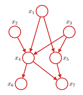
fig8_2. Download: PDF · SVGDefinition 8.1 (directed acyclic graphs and the factorisation they define) p. 362, (8.5)
A directed graph has nodes \(1,\dots,K\) and directed links \(j\to k\). A directed cycle is a sequence of links \(k_1\to k_2\to\dots\to k_m\to k_1\). A graph without directed cycles is a directed acyclic graph (DAG). \(\pa_k\) is the set of parents of \(k\); \(j\) is an ancestor of \(k\) (and \(k\) a descendant of \(j\)) if there is a directed path \(j\to\dots\to k\). An ordering of the nodes in which every link goes from a lower to a higher number is a topological ordering. A distribution \(p\) factorises over the DAG if
\[ p(\mathbf{x})=\prod_{k=1}^{K}p(x_k\given\pa_k) \tag{8.5} \]for some conditional distributions \(p(x_k\given\pa_k)\), one for each node, each normalised over \(x_k\) for every value of its parents. The set of all such \(p\) is denoted \(\mathcal{DF}\) (the book's "DF", for directed factorisation, p. 381).
Result 8.1 (acyclic means orderable; Exercise 8.2) p. 362
A finite directed graph has no directed cycles if and only if its nodes can be numbered so that every link goes from a lower to a higher number.
Proof
Ordering implies acyclic (the direction asked in Exercise 8.2). Along a directed cycle \(k_1\to k_2\to\dots\to k_m\to k_1\) the numbers would increase strictly at each step and yet return to the starting number, which is impossible.
Acyclic implies ordering. First, a finite DAG has a node without parents. Start at any node and step to one of its parents, then to a parent of that node, and so on. If every node had a parent, this could go on forever; after \(K+1\) steps some node would appear twice, and the steps between the two visits, read in the direction of the arrows, would be a directed cycle. So some node has no parents. Give it the number 1 and delete it with its links. What remains is still a DAG, so it has a node without parents (within the remaining graph): number it 2, delete it, and continue. When node \(k\) is numbered, all its parents in the original graph have already been deleted, so they carry smaller numbers. Every link therefore points from a lower to a higher number. ∎
Result 8.2 (the product (8.5) is a normalised distribution; Exercise 8.1) p. 362
Let \(q_k(x_k\given\pa_k)\ge0\) be normalised over \(x_k\) for each value of \(\pa_k\), and let the nodes be numbered topologically. Then \(p(\mathbf{x})=\prod_k q_k(x_k\given\pa_k)\) sums (integrates) to one. Moreover, for every \(k\),
\[ p(x_1,\dots,x_k)=\prod_{j=1}^{k}q_j(x_j\given\pa_j),\qquad p(x_k\given x_1,\dots,x_{k-1})=p(x_k\given\pa_k)=q_k(x_k\given\pa_k), \]so the factors are the conditional distributions of the joint, which justifies writing them as \(p(x_k\given\pa_k)\). Conversely, \(p\in\mathcal{DF}\) if and only if, in a topological ordering, \(p(x_k\given x_1,\dots,x_{k-1})\) depends on its conditioning variables only through \(\pa_k\).
Proof
Marginalise the last node. In a topological ordering \(x_K\) has no children (a child would carry a larger number). So \(x_K\) appears in exactly one factor, its own, and
\[ \sum_{x_K}\prod_{j=1}^{K}q_j(x_j\given\pa_j)=\Big[\prod_{j=1}^{K-1}q_j(x_j\given\pa_j)\Big]\sum_{x_K}q_K(x_K\given\pa_K)=\prod_{j=1}^{K-1}q_j(x_j\given\pa_j). \]The result is the same kind of product over the first \(K-1\) nodes, whose parents are all among \(x_1,\dots,x_{K-2}\). Repeating the step gives \(p(x_1,\dots,x_k)=\prod_{j\le k}q_j\) for every \(k\), and finally \(\sum_{x_1}q_1(x_1)=1\): the joint is normalised (for continuous variables replace sums by integrals; Fubini's theorem allows the order).
The factors are the conditionals. Dividing the formula for \(p(x_1,\dots,x_k)\) by the one for \(p(x_1,\dots,x_{k-1})\) gives \(p(x_k\given x_1,\dots,x_{k-1})\)
Converse. The chain rule (8.3) holds for every \(p\). If each factor \(p(x_k\given x_1,\dots,x_{k-1})\) is a function of \(x_k\) and \(\pa_k\) only, (8.3) is a product of the form (8.5). ∎
Filling the gap 8.1: why the graph must be acyclic p. 362
The book imposes acyclicity without saying what goes wrong otherwise. Two things fail.
Derivation
The product need not be normalised. Take two binary variables with links \(x_1\to x_2\) and \(x_2\to x_1\) (a directed cycle) and the "conditionals" \(q_1(x_1\given x_2)=[x_1=x_2]\), \(q_2(x_2\given x_1)=[x_2=x_1]\), each normalised. Their product is \([x_1=x_2]\), which sums to 2, not 1. With \(q_1(x_1\given x_2)=[x_1\ne x_2]\) instead, the product \([x_1\ne x_2][x_2=x_1]\) is identically zero. The marginalisation argument of Result 8.2 breaks down because no node appears in only one factor.
The factors need not be the conditionals. Even when a cyclic product happens to normalise, the \(q_k\) are in general not the conditionals of the resulting joint, so the graph would no longer describe a generative mechanism or allow ancestral sampling. A DAG is exactly the structure for which "multiply the conditionals" always produces a joint distribution whose conditionals are the factors. ∎
Nodes may stand for single variables, vectors or groups of variables. Every distribution factorises over a fully connected DAG (by (8.3)), so the interest of a graph is in the links it omits.
8.1.1 Example: Polynomial regression
pp. 362–365 In the Bayesian polynomial regression of Section 1.2.6 the random variables are the coefficient vector \(\mathbf{w}\) and the targets \(\mathbf{t}=(t_1,\dots,t_N)^\T\). Given \(\mathbf{w}\) the targets are generated independently, so
\[ p(\mathbf{t},\mathbf{w})=p(\mathbf{w})\prod_{n=1}^{N}p(t_n\given\mathbf{w}). \tag{8.6} \]The graph has an arrow from \(\mathbf{w}\) to each \(t_n\) (the book's Figure 8.3). A plate, a box labelled \(N\) around a single node \(t_n\), stands for \(N\) copies of everything inside it (Figure 8.4). Deterministic quantities (the inputs \(x_n\), the prior precision \(\alpha\), the noise variance \(\sigma^2\)) are drawn as small solid dots (Figure 8.5); with them written out, \(p(\mathbf{t},\mathbf{w}\given\mathbf{x},\alpha,\sigma^2)\)
Erratum. Some printings write \(p(\mathbf{w}\given\mathbf{T})\) on the left of (8.7); it should be \(\mathbf{t}\).
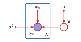
fig8_6. Download: PDF · SVGTo predict the target \(\widehat t\) at a new input \(\widehat x\) (the book's Figure 8.7) add the node \(\widehat t\) with parent \(\mathbf{w}\):
\[ p(\widehat t,\mathbf{t},\mathbf{w}\given\widehat x,\mathbf{x},\alpha,\sigma^2)=\Big[\prod_{n=1}^{N}p(t_n\given x_n,\mathbf{w},\sigma^2)\Big]p(\mathbf{w}\given\alpha)\,p(\widehat t\given\widehat x,\mathbf{w},\sigma^2), \tag{8.8} \]and the predictive distribution is \(p(\widehat t\given\widehat x,\mathbf{x},\mathbf{t},\alpha,\sigma^2)\)
Filling the gap 8.2: the predictive distribution read off the graph p. 365, (8.8)
The book writes the predictive distribution with a proportionality sign and refers to Chapter 3. Here is the normalising constant and the closed form.
Derivation
Drop the fixed parameters from the notation. By the sum rule and (8.8), \(p(\widehat t,\mathbf{t})\)
The training data enter only through the posterior of \(\mathbf{w}\); this is the conditional independence \(\widehat t\indep t_n\given\mathbf{w}\) of (8.36), read off the graph in Section 8.2.2. With \(p(\mathbf{w})\)
which is (1.69)–(1.72) of the book. ∎
8.1.2 Generative models
pp. 365–366 A DAG is also a recipe for simulation. Number the nodes topologically and draw each variable from its conditional distribution given the values already drawn for its parents.
Algorithm 8.1 (ancestral sampling) p. 365
- Number the nodes so that parents come before children (Result 8.1).
- For \(k=1,\dots,K\): draw \(\widehat x_k\sim p(x_k\given\pa_k)\) with the parents set to their drawn values \(\widehat{\pa}_k\) (all already available, because parents carry smaller numbers).
- Return \(\widehat{\mathbf{x}}\)
\({}=(\widehat x_1,\dots,\widehat x_K)\). To sample a marginal such as \(p(x_2,x_4)\), keep \(\widehat x_2,\widehat x_4\) and discard the rest.
Result 8.3 (ancestral sampling is exact) p. 365
The vector returned by Algorithm 8.1 has distribution \(p(\mathbf{x})=\prod_kp(x_k\given\pa_k)\), and any sub-vector of it has the corresponding marginal distribution.
Proof
For discrete variables, the probability of producing a particular \(\mathbf{x}\) is the probability of making each of the \(K\) draws correctly in turn, which by the product rule is
\[ \prod_{k=1}^{K}\Pr\big(\widehat x_k=x_k\given\widehat x_1=x_1,\dots,\widehat x_{k-1}=x_{k-1}\big)=\prod_{k=1}^{K}p(x_k\given\pa_k)=p(\mathbf{x}), \]since step \(k\) uses only the parent values. For continuous variables the same argument with conditional densities shows that \((\widehat x_1,\dots,\widehat x_k)\) has joint density \(\prod_{j\le k}p(x_j\given\pa_j)\) for every \(k\) (induction on \(k\)). A sub-vector of a random vector with distribution \(p\) has the marginal distribution by definition of a marginal. ∎
In applications the observed variables are usually the last nodes (leaves), and the latent variables above them make a complicated distribution over the observations out of simple, often exponential-family, conditionals. The book's Figure 8.8 is an example: an image depends on the identity of an object and on its position and orientation, which are a priori independent; recognising the object means computing its posterior given the image, integrating over position and orientation. Because such a graph describes how the data could have been produced (the causal process, Pearl, 1988), ancestral sampling produces synthetic "fantasy" data, and these models are called generative. The regression model of Figure 8.5 is not generative: it puts no distribution on the inputs \(x_n\). For drawing samples when some nodes are observed, see logic sampling and its acceptance rate in Chapter 11, Filling the gap 11.1.
8.1.3 Discrete variables
pp. 366–369 A variable with \(K\) states, coded 1-of-\(K\) as \(\mathbf{x}=(x_1,\dots,x_K)\) with one entry equal to 1, has distribution
\[ p(\mathbf{x}\given\bm\mu)=\prod_{k=1}^{K}\mu_k^{x_k}, \tag{8.9} \]with \(\mu_k\ge0\) and \(\sum_k\mu_k=1\), so \(K-1\) free parameters. A general joint distribution of two such variables needs \(\mu_{kl}=p(x_{1k}=1,x_{2l}=1)\): \(K^2-1\) free parameters. How many parameters does a graph need?
Result 8.4 (parameter counts for discrete DAGs) pp. 367–368, Figures 8.9, 8.10
If node \(k\) has \(K_k\) states, the conditional probability tables of a DAG have
\[ \#\text{parameters}=\sum_{k=1}^{M}(K_k-1)\prod_{j\in\pa_k}K_j \]free parameters. With \(M\) nodes of \(K\) states each this gives: \(K^M-1\) for the fully connected graph (exponential in \(M\)); \(M(K-1)\) for the graph without links (linear); \(K-1+(M-1)K(K-1)\) for the chain \(x_1\to x_2\to\dots\to x_M\) of Figure 8.10 (linear in \(M\), quadratic in \(K\)); and \(K^2-1\) for the chain with all transition tables tied to one table (Section 8.1.3, "sharing parameters").
Proof
The counting argument. A distribution on a set of \(n\) points is a vector in the probability simplex, which has \(n-1\) free coordinates (the last one is fixed by the sum to one). The table \(p(x_k\given\pa_k)\) consists of one distribution over the \(K_k\) states of \(x_k\) for each of the \(\prod_{j\in\pa_k}K_j\) configurations of the parents, and these distributions can be chosen independently of each other. Summing over nodes gives the formula.
Fully connected. Node \(k\) has \(k-1\) parents, so the count is \(\sum_{k=1}^{M}(K-1)K^{k-1}\)
No links. Each node has no parents: \(M(K-1)\) (Figure 8.9b gives \(2(K-1)\) for \(M=2\)).
Chain. \(x_1\) has no parents (\(K-1\)); each of \(x_2,\dots,x_M\) has one parent with \(K\) states (\(K(K-1)\) each).
Tied chain. \(p(x_1)\) needs \(K-1\) and the single shared table \(p(x_i\given x_{i-1})\) needs \(K(K-1)\), total \(K^2-1\), independent of \(M\). ∎
Graphs of intermediate connectivity interpolate between the two extremes: more general than full independence, cheaper than a general joint. A Bayesian treatment puts a Dirichlet prior on each table, which adds a parameter node as an extra parent of each discrete node (the book's Figure 8.11), or a single shared parameter node when the tables are tied (Figure 8.12).
Filling the gap 8.3: Dirichlet priors and tied parameters in a discrete DAG p. 368, Figures 8.11, 8.12
The book draws the Bayesian versions of the chain without computing anything. With complete data the posterior is a product of Dirichlet distributions, one per row of each table, and tying parameters simply pools the counts.
Derivation
Likelihood. Write \(\mu_{kjl}=p(x_k=l\given\pa_k=j)\) for state \(l\) of node \(k\) and parent configuration \(j\), and \(\bm\mu_{kj}=(\mu_{kj1},\dots,\mu_{kjK_k})\) for a row of the table. For \(N\) independent complete observations \(\mathbf{x}^{(1)},\dots,\mathbf{x}^{(N)}\), (8.5) gives
\[ p(\mathcal D\given\bm\mu)=\prod_{n=1}^{N}\prod_{k}\mu_{k,\pa_k^{(n)},x_k^{(n)}}=\prod_{k}\prod_{j}\prod_{l}\mu_{kjl}^{N_{kjl}}, \]where \(N_{kjl}\) counts the observations with \(x_k=l\) and \(\pa_k=j\). The likelihood is a product of separate multinomial kernels, one per row \(\bm\mu_{kj}\).
Posterior. Give the rows independent priors \(\bm\mu_{kj}\sim\Dir(\bm\alpha_{kj})\) (the parameter nodes of Figure 8.11). The posterior is proportional to prior times likelihood, which is again a product over rows of \(\prod_l\mu_{kjl}^{\alpha_{kjl}+N_{kjl}-1}\), so
\[ p(\bm\mu\given\mathcal D)=\prod_{k}\prod_{j}\Dir\big(\bm\mu_{kj}\given\bm\alpha_{kj}+\mathbf{N}_{kj}\big),\qquad \E[\mu_{kjl}\given\mathcal D]=\frac{\alpha_{kjl}+N_{kjl}}{\sum_{l'}(\alpha_{kjl'}+N_{kjl'})} \](toolkit: Dirichlet). The rows stay independent a posteriori. In graph terms: in Figure 8.11 every path between two parameter nodes \(\bm\mu_i\) and \(\bm\mu_j\) passes through an observed \(x\) node at which the arrows meet head-to-tail (for example \(\bm\mu_1\to x_1\to x_2\leftarrow\bm\mu_2\) is blocked at \(x_1\)), so the parameters are d-separated by the data (Section 8.2.2). With missing data this fails and the posterior no longer factorises (Chapter 9 deals with that case).
Tied tables (Figure 8.12). If \(p(x_i\given x_{i-1})=\mu_{x_{i-1}x_i}\) for all \(i=2,\dots,M\), the likelihood of one chain is \(\prod_l\mu_{1l}^{[x_1=l]}\prod_{j,l}\mu_{jl}^{N_{jl}}\) with \(N_{jl}=\sum_{i=2}^{M}[x_{i-1}=j,\,x_i=l]\), the number of transitions \(j\to l\) along the chain. With a Dirichlet prior on each row of the shared table the posterior row is \(\Dir(\bm\alpha_j+\mathbf N_j)\): tying replaces per-position counts by counts pooled over positions. This is how the transition matrix of a Markov chain or hidden Markov model is estimated (Chapter 13). ∎
A third way to control the number of parameters is a parametric conditional distribution. For binary parents \(x_1,\dots,x_M\) of a binary child \(y\) (Figure 8.13) a full table has \(2^M\) entries, but the logistic sigmoid of a linear combination,
\[ p(y=1\given x_1,\dots,x_M)=\sigma\Big(w_0+\sum_{i=1}^{M}w_ix_i\Big)=\sigma(\mathbf{w}^\T\mathbf{x}), \tag{8.10} \]with \(\sigma(a)=(1+e^{-a})^{-1}\), \(\mathbf{x}=(1,x_1,\dots,x_M)^\T\) and \(\mathbf{w}=(w_0,\dots,w_M)^\T\), needs only \(M+1\). The noisy-OR of Exercise 8.6 is another such model.
Filling the gap 8.4: what the logistic table (8.10) gives up p. 369, (8.10)
The book compares (8.10) with a diagonal covariance matrix: a restriction. Exactly which restriction? A full table is a sigmoid of a polynomial with all \(2^M\) interaction terms; (8.10) keeps the \(M+1\) terms of degree at most one.
Derivation
Every function on \(\{0,1\}^M\) is a multilinear polynomial. For \(S\subseteq\{1,\dots,M\}\) let \(x_S=\prod_{i\in S}x_i\) (with \(x_\varnothing=1\)). Every \(g:\{0,1\}^M\to\R\) can be written uniquely as
\[ g(\mathbf{x})=\sum_{S\subseteq\{1,\dots,M\}}w_S\,x_S,\qquad w_S=\sum_{U\subseteq S}(-1)^{|S\setminus U|}\,g(\mathbf{1}_U), \]where \(\mathbf{1}_U\) is the vector with ones exactly on \(U\). Uniqueness: there are \(2^M\) monomials and \(2^M\) points; evaluating \(\sum_Sw_Sx_S\) at \(\mathbf{1}_U\) gives \(\sum_{S\subseteq U}w_S\), a triangular system (order the sets by size) with ones on the diagonal, hence invertible. Its inverse is the stated alternating sum (Möbius inversion, proved in Result 8.13).
Apply it to the log-odds. If every entry of the table lies strictly between 0 and 1, \(g(\mathbf{x})\)
8.1.4 Linear-Gaussian models
pp. 370–372 Now let each node be a continuous variable whose conditional distribution is Gaussian with a mean linear in its parents:
\[ p(x_i\given\pa_i)=\N\Big(x_i\;\Big|\sum_{j\in\pa_i}w_{ij}x_j+b_i,\;v_i\Big). \tag{8.11} \]The log of the joint distribution is
\[ \ln p(\mathbf{x})=\sum_{i=1}^{D}\ln p(x_i\given\pa_i) \tag{8.12} \] \[ \phantom{\ln p(\mathbf{x})}=-\sum_{i=1}^{D}\frac{1}{2v_i}\Big(x_i-\sum_{j\in\pa_i}w_{ij}x_j-b_i\Big)^2+\const, \tag{8.13} \]a quadratic function of \(\mathbf{x}\), so \(p(\mathbf{x})\) is Gaussian. Equivalently, each variable is generated as
\[ x_i=\sum_{j\in\pa_i}w_{ij}x_j+b_i+\sqrt{v_i}\,\epsilon_i, \tag{8.14} \]with \(\epsilon_1,\dots,\epsilon_D\) independent standard normal (\(\E[\epsilon_i]=0\), \(\E[\epsilon_i\epsilon_j]=I_{ij}\)). Taking expectations,
\[ \E[x_i]=\sum_{j\in\pa_i}w_{ij}\E[x_j]+b_i, \tag{8.15} \]and multiplying the centred version of (8.14) by \(x_i-\E[x_i]\),
\[ \cov[x_i,x_j]=\E\Big[(x_i-\E[x_i])\Big\{\sum_{k\in\pa_j}w_{jk}(x_k-\E[x_k])+\sqrt{v_j}\,\epsilon_j\Big\}\Big]=\sum_{k\in\pa_j}w_{jk}\cov[x_i,x_k]+I_{ij}v_j. \tag{8.16} \]Result 8.5 (a linear-Gaussian DAG is a multivariate Gaussian) pp. 370–371, (8.11)–(8.16)
Number the nodes topologically and collect the weights in the matrix \(\mathbf{W}=(w_{ij})\) (zero unless \(j\in\pa_i\); strictly lower triangular), \(\mathbf{b}=(b_i)\) and \(\mathbf{V}=\diag(v_1,\dots,v_D)\). Then \(\mathbf{x}\sim\N(\bm\mu,\bm\Sigma)\) with
\[ \bm\mu=(\mathbf{I}-\mathbf{W})^{-1}\mathbf{b},\qquad \bm\Sigma=(\mathbf{I}-\mathbf{W})^{-1}\mathbf{V}(\mathbf{I}-\mathbf{W})^{-\T},\qquad \bm\Lambda=\bm\Sigma^{-1}=(\mathbf{I}-\mathbf{W})^\T\mathbf{V}^{-1}(\mathbf{I}-\mathbf{W}). \]The mean and covariance can be computed node by node with (8.15) and (8.16); (8.16) holds for \(i\le j\), and the other entries follow by symmetry. For \(i\ne j\), \(\Lambda_{ij}\ne0\) only if \(i\) and \(j\) are linked or are parents of a common child.
Proof
Gaussian. In matrix form (8.14) reads \(\mathbf{x}\)
Precision from (8.13). The sum in (8.13) is \(\frac12\big((\mathbf{I}-\mathbf{W})\mathbf{x}-\mathbf{b}\big)^\T\mathbf{V}^{-1}\big((\mathbf{I}-\mathbf{W})\mathbf{x}-\mathbf{b}\big)\). Its quadratic term is \(\frac12\mathbf{x}^\T\bm\Lambda\mathbf{x}\) with \(\bm\Lambda\) as stated, which confirms the precision. The constant in (8.13) is \(-\frac12\sum_i\ln(2\pi v_i)\), and \(|\bm\Lambda|=|\mathbf{V}|^{-1}\) because \(|\mathbf{I}-\mathbf{W}|=1\), so the constant is exactly the Gaussian normaliser \(\frac12\ln|\bm\Lambda|-\frac D2\ln2\pi\), as Result 8.2 promises.
The recursions. (8.15) is the expectation of (8.14). For (8.16), induction along the ordering shows that \(x_i-\E[x_i]\) is a linear combination of \(\epsilon_1,\dots,\epsilon_i\) only. Hence \(\E[(x_i-\E[x_i])\epsilon_j]\) is 0 for \(i\lt j\) (independence), and for \(i=j\) it equals \(\sqrt{v_j}\,\E[\epsilon_j^2]=\sqrt{v_j}\) (the other terms of \(x_j-\E[x_j]\) involve only \(\epsilon_k\), \(k\lt j\)). Multiplying by \(\sqrt{v_j}\) gives the term \(I_{ij}v_j\) of (8.16) for \(i\le j\). For \(i\gt j\) the formula is wrong in general: if \(x_i\) is a child of \(x_j\), then \(x_i\) depends on \(\epsilon_j\) and the missing term \(\sqrt{v_j}\E[(x_i-\E x_i)\epsilon_j]\)
Sparsity of \(\bm\Lambda\). \(\Lambda_{ij}\)
Filling the gap 8.5: the extreme cases and the three-node chain pp. 371–372, (8.17)–(8.18); Exercise 8.7
The book counts the parameters of the fully connected graph and says it corresponds to "a general symmetric covariance matrix". That every covariance matrix is attained, and uniquely, is the \(\mathbf{L}\mathbf{D}\mathbf{L}^\T\) factorisation. The chain of Figure 8.14 is then a two-line calculation.
Derivation
No links. \(\mathbf{W}=\mathbf 0\), so \(\bm\mu=\mathbf b\) and \(\bm\Sigma=\diag(v_1,\dots,v_D)\): \(2D\) parameters, \(D\) independent univariate Gaussians.
Fully connected. Row \(i\) of \(\mathbf W\) has \(i-1\) free entries, in total \(\frac{D^2-D}{2}=\frac{D(D-1)}2\); with the \(D\) variances this is \(\frac{D(D+1)}2\), the number of free entries of a symmetric \(D\times D\) matrix. Every positive definite \(\bm\Sigma\) is attained: write its Cholesky factorisation \(\bm\Sigma=\mathbf{C}\mathbf{C}^\T\) and set \(\mathbf{L}=\mathbf{C}\,\diag(\mathbf C)^{-1}\) (unit lower triangular) and \(\mathbf{V}=\diag(\mathbf C)^2\), so \(\bm\Sigma=\mathbf{L}\mathbf{V}\mathbf{L}^\T\). Choose \(\mathbf{W}=\mathbf{I}-\mathbf{L}^{-1}\) (strictly lower triangular, because the inverse of a unit lower triangular matrix is unit lower triangular) and \(\mathbf b=\mathbf{L}^{-1}\bm\mu\). By Result 8.5 this graph has mean \(\bm\mu\) and covariance \(\bm\Sigma\). The parameters are unique (the \(\mathbf{L}\mathbf{D}\mathbf{L}^\T\) factorisation is unique) and have a statistical meaning: \(w_{i1},\dots,w_{i,i-1}\) are the coefficients of the regression of \(x_i\) on \(x_1,\dots,x_{i-1}\), and \(v_i\) is the residual (conditional) variance.
The chain \(x_1\to x_2\to x_3\) (Figure 8.14, no link between \(x_1\) and \(x_3\)). By (8.15): \(\mu_1=b_1\), \(\mu_2=b_2+w_{21}\mu_1\), \(\mu_3=b_3+w_{32}\mu_2\), which is
\[ \bm\mu=\big(b_1,\;b_2+w_{21}b_1,\;b_3+w_{32}b_2+w_{32}w_{21}b_1\big)^\T. \tag{8.17} \]By (8.16) with \(i\le j\): \(\Sigma_{11}=v_1\); \(\Sigma_{12}=w_{21}\Sigma_{11}=w_{21}v_1\); \(\Sigma_{22}\)
The missing link does not make \(\Sigma_{13}\) zero (\(x_1\) and \(x_3\) are correlated through \(x_2\)); it makes the precision entry zero: from Result 8.5,
\[ \bm\Lambda=\begin{pmatrix}\frac1{v_1}+\frac{w_{21}^2}{v_2} & -\frac{w_{21}}{v_2} & 0\\ -\frac{w_{21}}{v_2} & \frac1{v_2}+\frac{w_{32}^2}{v_3} & -\frac{w_{32}}{v_3}\\ 0 & -\frac{w_{32}}{v_3} & \frac1{v_3}\end{pmatrix}, \]and \(\Lambda_{13}=0\) means \(x_1\indep x_3\given x_2\) (for a Gaussian, the conditional covariance of \((x_1,x_3)\) given \(x_2\) is the inverse of the corresponding \(2\times2\) block of \(\bm\Lambda\), which is diagonal). All three matrices were checked symbolically. ∎
p. 372 The same construction works when the nodes are Gaussian vectors,
\[ p(\mathbf{x}_i\given\pa_i)=\N\Big(\mathbf{x}_i\;\Big|\sum_{j\in\pa_i}\mathbf{W}_{ij}\mathbf{x}_j+\mathbf{b}_i,\;\bm\Sigma_i\Big), \tag{8.19} \]with matrices \(\mathbf{W}_{ij}\) (rectangular if the dimensions differ): stacking the nodes, \(\mathbf{I}-\mathbf{W}\) is block lower triangular with identity blocks on the diagonal, hence invertible, and the proof of Result 8.5 goes through with \(\mathbf{V}=\diag(\bm\Sigma_1,\dots,\bm\Sigma_D)\). The conjugate Gaussian prior on the mean of a Gaussian (Section 2.3.6) is the two-node case \(\bm\mu\to\mathbf{x}\); a Gaussian prior on the prior mean (a hyperprior) adds a third node above it, giving a hierarchical Bayesian model that is still jointly Gaussian. Probabilistic PCA, factor analysis (Chapter 12) and linear dynamical systems (Chapter 13) are linear-Gaussian models of this kind (Roweis and Ghahramani, 1999).
8.2 Conditional independence
pp. 372–373 If the conditional distribution of \(a\) given \(b\) and \(c\) does not depend on \(b\),
\[ p(a\given b,c)=p(a\given c), \tag{8.20} \]then, by the product rule,
\[ p(a,b\given c)=p(a\given b,c)\,p(b\given c)=p(a\given c)\,p(b\given c). \tag{8.21} \]Definition 8.2 (conditional independence) pp. 372–373, (8.20)–(8.22)
Variables (or sets of variables) \(a\) and \(b\) are conditionally independent given \(c\), written
\[ a\indep b\given c, \tag{8.22} \]if \(p(a,b\given c)=p(a\given c)\,p(b\given c)\) for all values of \(a,b\) and every value of \(c\) with \(p(c)\gt0\). Equivalently, (8.20) holds whenever \(p(b,c)\gt0\). With \(c\) empty, \(a\indep b\given\varnothing\) is ordinary independence. The concept is studied systematically by Dawid (1980); the notation is Dawid's (1979).
The requirement "for every value of \(c\)" matters: a dependence for a single value of \(c\) breaks the property. The following criterion makes most proofs in this chapter one line long.
Result 8.6 (the factorisation criterion, decomposition and weak union; Exercise 8.8)
(a) \(a\indep b\given c\) if and only if there are nonnegative functions \(g,h\) with \(p(a,b,c)=g(a,c)\,h(b,c)\) for all \(a,b,c\).
(b) Decomposition (Exercise 8.8): if \(a\indep(b,d)\given c\) then \(a\indep b\given c\).
(c) Weak union: if \(a\indep(b,d)\given c\) then \(a\indep b\given(c,d)\).
Proof
(a) If \(a\indep b\given c\), take \(g(a,c)=p(a\given c)\) and \(h(b,c)=p(b,c)\) when \(p(c)\gt0\), and \(h(b,c)=0\) when \(p(c)=0\) (then \(p(a,b,c)=0\) too). Conversely, suppose \(p(a,b,c)=g(a,c)h(b,c)\) and put \(G(c)=\sum_ag(a,c)\), \(H(c)=\sum_bh(b,c)\). Summing over \(a\), over \(b\), or over both gives \(p(b,c)=G(c)h(b,c)\), \(p(a,c)=g(a,c)H(c)\) and \(p(c)=G(c)H(c)\). For \(p(c)\gt0\),
\[ p(a\given c)\,p(b\given c)=\frac{g(a,c)H(c)\;G(c)h(b,c)}{G(c)^2H(c)^2}=\frac{g(a,c)h(b,c)}{G(c)H(c)}=\frac{p(a,b,c)}{p(c)}=p(a,b\given c). \](b) By (a), \(p(a,b,d,c)=g(a,c)h(b,d,c)\). Summing over \(d\): \(p(a,b,c)=g(a,c)\,\widetilde h(b,c)\) with \(\widetilde h=\sum_dh\), so \(a\indep b\given c\) by (a). (The book's solution sums \(p(a,b,d\given c)=p(a\given c)p(b,d\given c)\) over \(d\), which is the same argument.)
(c) The same factorisation \(p(a,b,d,c)=g(a,c)h(b,d,c)\) reads, with \((c,d)\) as the conditioning variable, \(g'(a,(c,d))\,h(b,(c,d))\) where \(g'\) ignores \(d\); by (a), \(a\indep b\given(c,d)\). ∎
Testing a conditional independence by manipulating the sum and product rules is laborious. The point of the graph is that the independences can be read off it, by a criterion called d-separation (Pearl, 1988). The three examples below contain all the ideas.
8.2.1 Three example graphs
pp. 373–376 By (8.5), the three graphs of Figure 8.15 (top row) have the joint distributions
\[ \text{tail-to-tail } (a\leftarrow c\to b):\qquad p(a,b,c)=p(a\given c)\,p(b\given c)\,p(c), \tag{8.23} \] \[ \text{head-to-tail } (a\to c\to b):\qquad p(a,b,c)=p(a)\,p(c\given a)\,p(b\given c), \tag{8.26} \] \[ \text{head-to-head } (a\to c\leftarrow b):\qquad p(a,b,c)=p(a)\,p(b)\,p(c\given a,b). \tag{8.28} \]The names describe how the two arrows of the path \(a - c - b\) meet at \(c\): at their tails, one head and one tail, or at their heads. Marginalising (8.23) over \(c\) gives
\[ p(a,b)=\sum_c p(a\given c)\,p(b\given c)\,p(c), \tag{8.24} \]which in general is not \(p(a)p(b)\), so
\[ a\nindep b\given\varnothing; \tag{8.25} \]the same holds for the head-to-tail graph,
\[ a\nindep b\given\varnothing, \tag{8.27} \]whereas for the head-to-head graph \(\sum_c p(c\given a,b)=1\) gives \(p(a,b)=p(a)p(b)\):
\[ a\indep b\given\varnothing. \tag{8.29} \]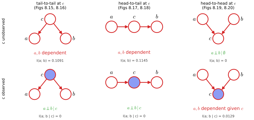
fig8_15. Download: PDF · SVGResult 8.7 (the three basic graphs) pp. 373–376, (8.23)–(8.29)
For every distribution that factorises over the graph:
- tail-to-tail \(a\leftarrow c\to b\) and head-to-tail \(a\to c\to b\): \(a\indep b\given c\);
- head-to-head \(a\to c\leftarrow b\): \(a\indep b\given\varnothing\).
The opposite statements do not follow from the graph: there are distributions factorising over the first two graphs with \(a\nindep b\given\varnothing\), and over the third with \(a\nindep b\given c\).
Proof, with numerical counterexamples
Tail-to-tail. (8.23) is of the form \(g(a,c)h(b,c)\) with \(g=p(a\given c)\), \(h=p(b\given c)p(c)\), so \(a\indep b\given c\) by Result 8.6(a). Directly: \(p(a,b\given c)\)
Head-to-tail. (8.26) is \(g(a,c)h(b,c)\) with \(g=p(a)p(c\given a)\), \(h=p(b\given c)\), so \(a\indep b\given c\). (Equivalently, by Bayes' theorem \(p(a)p(c\given a)=p(c)p(a\given c)\), so \(p(a,b\given c)=p(a\given c)p(b\given c)\), as on p. 375.) Marginally, \(p(a,b)\)
Head-to-head. Marginal independence was shown in (8.29). Given \(c\), \(p(a,b\given c)=p(a)p(b)p(c\given a,b)/p(c)\), and \(p(c\given a,b)\) need not split into a function of \((a,c)\) times a function of \((b,c)\). Counterexample: \(a,b\) independent fair bits and \(c=a\oplus b\) (exclusive or). Given \(c=0\), \((a,b)\) is \((0,0)\) or \((1,1)\) with probability \(\frac12\) each, so \(p(a=1\given c=0)=p(b=1\given c=0)=\frac12\) but \(p(a=1,b=1\given c=0)=\frac12\ne\frac14\). Knowing \(c\) and \(a\) determines \(b\). The fuel gauge below is a less extreme example. ∎
Graphical summary pp. 374–376. A path through a tail-to-tail or head-to-tail node is open when the node is unobserved and blocked when it is observed. A path through a head-to-head node is blocked when the node is unobserved and becomes open when it is observed. A node \(y\) is a descendant of \(x\) if there is a directed path from \(x\) to \(y\); observing a descendant of a head-to-head node also opens the path.
Result 8.8 (observing a descendant of a head-to-head node; Exercise 8.10) p. 376, Figure 8.54
In the graph \(a\to c\leftarrow b\), \(c\to d\) (Figure 8.54) every factorising distribution has \(a\indep b\given\varnothing\), but in general \(a\nindep b\given d\).
Proof
The joint is \(p(a)p(b)p(c\given a,b)p(d\given c)\). Summing over \(d\) and then \(c\) gives \(p(a,b)=p(a)p(b)\). Given \(d\),
\[ p(a,b\given d)=\frac{p(a)\,p(b)\sum_cp(c\given a,b)\,p(d\given c)}{p(d)}, \]and the sum is an arbitrary-looking function of \((a,b,d)\). Counterexample: \(a,b\) fair independent bits, \(c=a\oplus b\), and \(d\) a noisy copy of \(c\), \(p(d=c\given c)=0.9\). Then \(p(a,b,d=0)=\frac14\cdot0.9\) if \(a=b\) and \(\frac14\cdot0.1\) otherwise, so \(p(d=0)=\frac12\), \(p(a=1\given d=0)=p(b=1\given d=0)=\frac12\), but \(p(a=1,b=1\given d=0)=0.45\ne0.25\). The report \(d\) carries information about \(c\), and that is enough to couple \(a\) and \(b\). ∎
Explaining away: the fuel gauge pp. 376–378, (8.30)–(8.33)
Battery \(B\) (charged 1, flat 0) and fuel tank \(F\) (full 1, empty 0) are independent a priori, \(p(B=1)=p(F=1)=0.9\), and both influence the gauge \(G\) (reads full 1, empty 0) through
| \((B,F)\) | \((1,1)\) | \((1,0)\) | \((0,1)\) | \((0,0)\) |
|---|---|---|---|---|
| \(p(G=1\given B,F)\) | 0.8 | 0.2 | 0.2 | 0.1 |
| \(p(G=0\given B,F)\) | 0.2 | 0.8 | 0.8 | 0.9 |
The graph \(B\to G\leftarrow F\) is head-to-head at \(G\). Observing \(G=0\) makes an empty tank more likely; then learning that the battery is flat makes it less likely again, because the flat battery already explains the reading:
\[ p(G=0)=\sum_{B\in\{0,1\}}\sum_{F\in\{0,1\}}p(G=0\given B,F)\,p(B)\,p(F)=0.315, \tag{8.30} \] \[ p(G=0\given F=0)=\sum_{B\in\{0,1\}}p(G=0\given B,F=0)\,p(B)=0.81, \tag{8.31} \] \[ p(F=0\given G=0)=\frac{p(G=0\given F=0)\,p(F=0)}{p(G=0)}\simeq0.257, \tag{8.32} \] \[ p(F=0\given G=0,B=0)=\frac{p(G=0\given B=0,F=0)\,p(F=0)}{\sum_{F\in\{0,1\}}p(G=0\given B=0,F)\,p(F)}\simeq0.111. \tag{8.33} \]Filling the gap 8.6: the fuel-gauge numbers pp. 377–378, (8.30)–(8.33)
The book quotes the four numbers. Here is the arithmetic, why \(p(B=0)\) cancels in (8.33), and the companion value for a charged battery.
Derivation
(8.30). The four terms \(p(G=0\given B,F)p(B)p(F)\) are
\[ \underbrace{0.2\cdot0.9\cdot0.9}_{B=1,F=1}+\underbrace{0.8\cdot0.9\cdot0.1}_{B=1,F=0}+\underbrace{0.8\cdot0.1\cdot0.9}_{B=0,F=1}+\underbrace{0.9\cdot0.1\cdot0.1}_{B=0,F=0}=0.162+0.072+0.072+0.009=0.315. \](8.31). Because \(B\) and \(F\) are independent, \(p(B\given F=0)=p(B)\), and the sum rule gives \(p(G=0\given F=0)\)
(8.32). Bayes' theorem: \(p(F=0\given G=0)\)
(8.33). Condition on both observations: \(p(F\given G=0,B=0)\)
Why this is dependence. A priori \(F\indep B\) (8.29). If \(F\indep B\given G\) held, \(p(F=0\given G=0,B)\) would not depend on \(B\). But it equals \(0.111\) for \(B=0\) and, by the same formula,
\[ p(F=0\given G=0,B=1)=\frac{0.8\cdot0.1}{0.8\cdot0.1+0.2\cdot0.9}=\frac{0.08}{0.26}=\frac4{13}\approx0.308 \]for \(B=1\): a charged battery makes the empty reading more credible. Averaging the two with \(p(B\given G=0)\) (which equals \(9/35\) for \(B=0\), by the symmetry of the numbers) recovers \(9/35\). The probability 0.111 still exceeds the prior 0.1: the gauge reading still carries some evidence for an empty tank. All values were checked in exact rational arithmetic. ∎
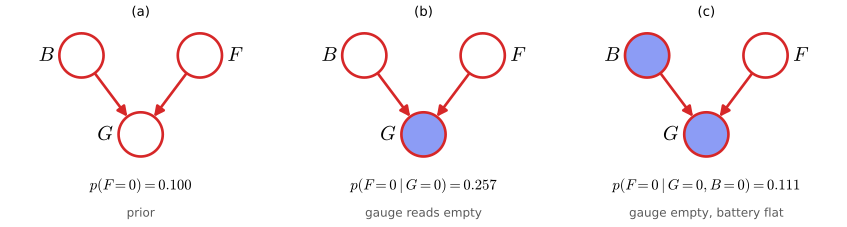
fig8_21. Download: PDF · SVGExercise 8.11 replaces the gauge by a driver's unreliable report of it, a descendant of \(G\); explaining away persists (solution).
8.2.2 D-separation
pp. 378–379 The general rule replaces the single middle node by every node on every path.
Definition 8.3 (blocked paths and d-separation; Pearl, 1988) p. 378
Let \(A\), \(B\), \(C\) be disjoint sets of nodes of a DAG (their union need not be all nodes). A path is a sequence of distinct nodes, each linked to the next, regardless of the direction of the links. An interior node of a path is head-to-head (a collider) on it if both links of the path at that node point into it. A path is blocked by \(C\) if it contains a node such that either
(a) the arrows meet head-to-tail or tail-to-tail at the node, and the node is in \(C\); or
(b) the arrows meet head-to-head at the node, and neither the node nor any of its descendants is in \(C\).
\(A\) is d-separated from \(B\) by \(C\) if every path from a node of \(A\) to a node of \(B\) is blocked. A path that is not blocked is called active (or d-connecting).
In Figure 8.22(a), with \(C=\{c\}\), the only path from \(a\) to \(b\) is \(a\to e\leftarrow f\to b\). It is not blocked at \(f\) (tail-to-tail but unobserved), nor at \(e\) (head-to-head, and its descendant \(c\) is observed). So \(a\indep b\given c\) does not follow from the graph. In Figure 8.22(b), with \(C=\{f\}\), the same path is blocked at \(f\) (tail-to-tail and observed), and also at \(e\) (head-to-head with neither \(e\) nor \(c\) observed), so \(a\indep b\given f\) for every distribution that factorises over the graph. With nothing observed, the path is blocked at \(e\) and \(a\indep b\given\varnothing\).
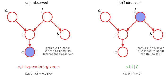
fig8_22. Download: PDF · SVGThe book states that d-separation implies conditional independence for every factorising distribution and refers to Lauritzen (1996) for a proof (p. 373). It also describes the graph as a filter (p. 381, Figure 8.25): the set of distributions passed by the factorisation filter, \(\mathcal{DF}\), equals the set passed by the filter "satisfy every d-separation statement". Both claims are proved below; the proof is the main piece of theory missing from the chapter.
Result 8.9 (the d-separation theorem) pp. 378, 381–382, Figure 8.25
Let \(G\) be a DAG and \(A,B,C\) disjoint sets of its nodes.
(a) Soundness. If \(C\) d-separates \(A\) from \(B\), then \(A\indep B\given C\) for every \(p\in\mathcal{DF}\).
(b) The two filters agree. A distribution \(p\) satisfies \(A\indep B\given C\) for every d-separation statement of \(G\) if and only if \(p\in\mathcal{DF}\).
(c) Completeness (stated without proof). If \(C\) does not d-separate \(A\) from \(B\), there is a \(p\in\mathcal{DF}\) with \(A\nindep B\given C\); for discrete variables, the tables for which such a dependence disappears form a set of Lebesgue measure zero (Meek, 1995). So d-separation lists exactly the independences that hold for all distributions of the graph, and generically no others.
Proof of (a) and (b)
Write \(\an(S)\) for the set of nodes of \(S\) together with all their ancestors. The proof of (a) goes through an undirected graph and has three steps (Lauritzen et al., 1990).
Step 1: marginal on an ancestral set. Let \(H=\an(A\cup B\cup C)\). Then \(p(\mathbf{x}_H)=\prod_{k\in H}p(x_k\given\pa_k)\). Indeed, \(H\) contains the parents of its nodes. Among the nodes outside \(H\), take the last one \(v\) in a topological ordering. A child of \(v\) inside \(H\) would make \(v\) an ancestor of \(H\), hence a member of \(H\); a child outside \(H\) would come after \(v\). So \(v\) has no children, appears only in its own factor, and summing over \(x_v\) removes that factor (as in Result 8.2). Repeat until only \(H\) is left.
Step 2: an undirected factorisation. Let \(M\) be the moral graph of \(G\) restricted to \(H\): join every pair of parents of a common child by an undirected link, then drop all arrow heads (Section 8.3.4). Each factor \(p(x_k\given\pa_k)\) depends on \(\{k\}\cup\pa_k\), a fully connected set in \(M\). If \(C\) separates \(A\) from \(B\) in \(M\) (every path from \(A\) to \(B\) in \(M\) passes through \(C\)), then Result 8.12 (a three-line argument in Section 8.3.2, independent of this proof) gives \(A\indep B\given C\) under \(p(\mathbf{x}_H)\), and therefore under \(p\), since \(A,B,C\subseteq H\).
Step 3: d-separation in \(G\) implies separation in \(M\). We prove the contrapositive: a path in \(M\) from \(A\) to \(B\) avoiding \(C\) yields an active path in \(G\). Call a trail a sequence of nodes, each linked in \(G\) to the next, in which nodes may repeat; a trail is active if every non-collider occurrence is outside \(C\) and every collider occurrence is in \(\an(C)\) (that is, the node or one of its descendants is in \(C\)).
(i) From \(M\) to a trail. Let \(a=v_0 - v_1 - \dots - v_n=b\) be the path in \(M\), with no \(v_i\) in \(C\). Each link of \(M\) is either a link of \(G\) or a moral link between two parents of a child \(w\in H\); replace the latter by \(v_i\to w\leftarrow v_{i+1}\). This gives a trail in \(G\) whose non-collider occurrences are all among the \(v_i\) (so outside \(C\)) and whose colliders all lie in \(H=\an(A\cup B\cup C)\).
(ii) Removing bad colliders. Among all trails from \(A\) to \(B\) whose non-colliders avoid \(C\) and whose colliders lie in \(\an(A\cup B\cup C)\), choose one with the fewest collider occurrences outside \(\an(C)\). Suppose it has such a collider \(w\). Then \(w\in\an(A\cup B)\), so there is a directed path \(w\to\dots\to t\) with \(t\in A\cup B\), and no node of it is in \(C\) (otherwise \(w\in\an(C)\)). If \(t\in A\), start a new trail at \(t\), run backwards along this directed path to \(w\), then continue along the old trail from \(w\) to its end in \(B\). On the new piece every node, including \(w\), is a non-collider (the links run in one direction), and none is in \(C\); the rest of the trail keeps its old colliders minus \(w\). If \(t\in B\), keep the old trail from its start to \(w\) and then follow the directed path to \(t\). Either way there is one bad collider fewer, a contradiction. So the chosen trail is active.
(iii) From an active trail to an active path. If a node \(v\) occurs twice on an active trail, cut out the stretch between the two occurrences. The new occurrence of \(v\) keeps the link before the first occurrence and the link after the second. If \(v\in C\), both old occurrences were colliders (non-colliders avoid \(C\)), so both kept links point into \(v\): the new occurrence is a collider in \(C\subseteq\an(C)\). If \(v\notin C\) and the new occurrence is a non-collider, nothing is needed. Finally let \(v\notin C\) with the new occurrence a collider, so both kept links point into \(v\). If either old occurrence was a collider, \(v\in\an(C)\) and we are done. Otherwise the first old occurrence, entered by a link pointing into \(v\), was left by a link pointing away from \(v\); likewise the second was entered by a link pointing away from \(v\). So the cut-out stretch starts with \(v\to\cdot\) and ends with \(\cdot\leftarrow v\). Walking along it, the first link traversed against its arrow is preceded by a collider of the trail, which is reached from \(v\) by a directed path; that collider is in \(\an(C)\) because the trail is active, hence so is \(v\). In every case the shorter trail is still active. Repeating the cut, we end with an active path from \(A\) to \(B\): \(C\) does not d-separate \(A\) from \(B\).
Together: d-separation in \(G\) gives separation in \(M\) (Step 3), which gives \(A\indep B\given C\) (Steps 1 and 2). This proves (a).
(b) "If" is (a). For "only if", number the nodes topologically and let \(P_k=\{1,\dots,k-1\}\). Claim: \(\pa_k\) d-separates \(k\) from \(P_k\setminus\pa_k\). Take a path from \(k\) to \(u\in P_k\setminus\pa_k\). If its first link is \(j\to k\), then \(j\in\pa_k\), \(j\ne u\), and the link leaves \(j\) by its tail, so \(j\) is not head-to-head: the path is blocked at \(j\in\pa_k\). If its first link is \(k\to y_1\), follow the path \(k\to y_1, y_2,\dots,u\). Not all its links can point forwards, since \(u\) precedes \(k\) and so is not a descendant of \(k\). At the first link that points backwards, the node just before it is head-to-head and is a descendant of \(k\); neither it nor any of its descendants is in \(\pa_k\) (that would close a directed cycle). So the path is blocked there. Hence the claim. If \(p\) satisfies all d-separation statements, it satisfies these, so \(p(x_k\given\mathbf{x}_{P_k})=p(x_k\given\pa_k)\) for every \(k\), and \(p\in\mathcal{DF}\) by Result 8.2. ∎
Two remarks complete the picture. First, the fully connected DAG has no d-separation statements and \(\mathcal{DF}\) is everything; the empty graph lets through only fully factorised distributions. A fully factorised distribution passes every filter: \(\mathcal{DF}\) contains distributions with more independences than the graph shows. Second, d-separation can be tested in time linear in the size of the graph (Geiger, Verma and Pearl, 1990), which is what the demonstration does.
Parameters p. 379. Deterministic parameters (solid dots such as \(\alpha\), \(\sigma^2\) in Figure 8.5) behave like observed nodes. They have no parents, so every path through them is tail-to-tail there and blocked: they never affect d-separation.
Independent identically distributed data pp. 379–380. In the graph \(\mu\to x_n\), \(n=1,\dots,N\) (the book's Figure 8.23), the unique path between \(x_i\) and \(x_j\) is tail-to-tail at \(\mu\). Given \(\mu\) it is blocked, so
\[ p(\mathcal D\given\mu)=\prod_{n=1}^{N}p(x_n\given\mu); \tag{8.34} \]with \(\mu\) unobserved the path is open and
\[ p(\mathcal D)=\int_{-\infty}^{\infty}p(\mathcal D\given\mu)\,p(\mu)\,\d\mu\ne\prod_{n=1}^{N}p(x_n). \tag{8.35} \]Erratum. Some printings have 0 as the lower limit of the integral in (8.35); it should be \(-\infty\).
For example, with \(\mu\sim\N(\mu_0,\sigma_0^2)\) and \(x_n\given\mu\sim\N(\mu,\sigma^2)\), write \(x_n=\mu+\sigma\epsilon_n\): then \(\cov[x_i,x_j]=\var[\mu]=\sigma_0^2\) for \(i\ne j\), so \(p(\mathcal D)\)
which is why the training data can be discarded once the posterior over \(\mathbf w\) is known (Filling the gap 8.2).
Naive Bayes pp. 380–381, Figure 8.24
A class label \(\mathbf z\) (1-of-\(K\), prior \(p(\mathbf z\given\bm\mu)\)) is the single parent of every feature \(x_1,\dots,x_D\). Every path between \(x_i\) and \(x_j\) is tail-to-tail at \(\mathbf z\): the features are independent given the class but dependent marginally.
Filling the gap 8.7: fitting and using naive Bayes pp. 380–381
The book says that maximum likelihood fits "each class separately" and that the marginal does not factorise. Both in formulas.
Derivation
Fitting. With labelled data \(\{(\mathbf x_n,\mathbf z_n)\}\) and class-conditional feature models \(p(x_i\given\bm\theta_{ik})\), the graph gives
\[ \ln p(\mathcal D)=\sum_{n}\sum_{k}z_{nk}\Big[\ln\mu_k+\sum_{i=1}^{D}\ln p(x_{ni}\given\bm\theta_{ik})\Big]=\sum_k N_k\ln\mu_k+\sum_{k}\sum_{i}\sum_{n:\,z_{nk}=1}\ln p(x_{ni}\given\bm\theta_{ik}). \]The first sum is maximised under \(\sum_k\mu_k=1\) by \(\mu_k=N_k/N\) (toolkit: Lagrange multipliers); each \(\bm\theta_{ik}\) appears in exactly one term of the double sum and is fitted to feature \(i\) of the class-\(k\) points alone: \(KD\) one-dimensional problems. For Gaussian features, \(\bm\theta_{ik}=(m_{ik},s^2_{ik})\) are the class-wise sample mean and variance (divisor \(N_k\)), i.e. one Gaussian per class with a diagonal covariance (axis-aligned elliptical contours). Binary features get Bernoulli models, and mixed feature types are no problem because each feature has its own model.
Classifying. Bayes' theorem gives \(p(z_k=1\given\mathbf x)\)
The marginal. \(p(\mathbf x)\)
The Markov blanket pp. 382–383, Figure 8.26
What is the conditional distribution of one node given all the others? Using (8.5),
\[ p(x_i\given\mathbf{x}_{\{j\ne i\}})=\frac{p(x_1,\dots,x_D)}{\int p(x_1,\dots,x_D)\,\d x_i}=\frac{\prod_kp(x_k\given\pa_k)}{\int\prod_kp(x_k\given\pa_k)\,\d x_i}, \]and every factor that does not contain \(x_i\) cancels.
Result 8.10 (the Markov blanket of a directed graph; Exercise 8.9) pp. 382–383
Let \(\mathrm{ch}_i\) be the children of node \(i\). Then
\[ p(x_i\given\mathbf{x}_{\{j\ne i\}})=\frac{p(x_i\given\pa_i)\prod_{k\in\mathrm{ch}_i}p(x_k\given\pa_k)}{\int p(x_i\given\pa_i)\prod_{k\in\mathrm{ch}_i}p(x_k\given\pa_k)\,\d x_i}, \]which depends only on the Markov blanket of \(i\): its parents, its children and its co-parents (the other parents of its children). Equivalently, the Markov blanket d-separates \(x_i\) from all remaining nodes. It is the smallest set with this property for a generic distribution of the graph: dropping a co-parent leaves an active path through a child (explaining away).
Proof
The formula. A factor \(p(x_k\given\pa_k)\) contains \(x_i\) exactly when \(k=i\) or \(i\in\pa_k\) (i.e. \(k\in\mathrm{ch}_i\)). All other factors are constant in \(x_i\), can be taken out of the integral, and cancel between numerator and denominator. The remaining factors involve \(x_i\), \(\pa_i\), the children \(x_k\) and their parents \(\pa_k\), which are \(x_i\) and the co-parents.
D-separation (Exercise 8.9). Let \(C\) be the blanket and consider a path from \(i\) to a node \(u\) outside \(C\cup\{i\}\). (1) If it starts with \(j\to i\), \(j\) is a parent, in \(C\), and not head-to-head on the path (the link leaves \(j\) by its tail): blocked. (2) If it starts with \(i\to k\) and continues \(k\to\cdot\), then \(k\in C\) is head-to-tail: blocked. (3) If it starts \(i\to k\leftarrow j\), then \(j\) is a co-parent in \(C\); the path leaves \(j\) by a link that, at \(j\), meets \(j\to k\) tail-to-tail or head-to-tail, so it is blocked at \(j\) (\(j\ne u\) because \(u\notin C\)). Every path is blocked, so Result 8.9 gives \(x_i\indep\mathbf{x}_{\text{rest}}\given\mathbf{x}_C\).
Why the co-parents are needed. If a co-parent \(j\) (with common child \(k\)) is left out, the path \(i\to k\leftarrow j\) has an observed head-to-head node and is active; by Result 8.9(c) the dependence is present for generic tables. ∎
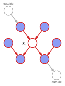
fig8_26. Download: PDF · SVGThe Markov blanket is what Gibbs sampling needs (Chapter 11, Section 11.3): each update draws a node from the conditional above, which involves only a handful of factors.
8.3 Markov random fields
p. 383 A Markov random field (Markov network, undirected graphical model; Kindermann and Snell, 1980) has one node per variable or group of variables and undirected links. As for directed graphs, the graph specifies both a factorisation and a set of conditional independences; this time it is simpler to start with the independences.
8.3.1 Conditional independence properties
pp. 383–385 Removing the arrows removes the asymmetry between parents and children, and with it the head-to-head subtlety: in an undirected graph a path is blocked exactly when it passes through an observed node.
Definition 8.4 (separation and the Markov properties of an undirected graph) pp. 384–385, (8.37)–(8.38)
In an undirected graph, a set \(C\) separates \(A\) from \(B\) (disjoint sets) if every path from a node of \(A\) to a node of \(B\) passes through a node of \(C\); equivalently, after deleting the nodes of \(C\) and their links, no node of \(A\) is connected to a node of \(B\). A distribution \(p\) has
- the global Markov property if \(C\) separates \(A\) from \(B\) implies
- the local Markov property if every node is independent of all non-neighbours given its neighbours, \(x_i\indep\mathbf{x}_{\text{rest}}\given\mathbf{x}_{\mathrm{ne}(i)}\) (the Markov blanket of an undirected graph is the set of neighbours, Figure 8.28);
- the pairwise Markov property if for every pair \(i,j\) that is not linked,
The set of distributions with the global Markov property is the book's \(\mathcal{UI}\) (p. 387).
Result 8.11 (global implies local implies pairwise) pp. 384–385
For every distribution: global Markov \(\Rightarrow\) local Markov \(\Rightarrow\) pairwise Markov. For strictly positive distributions all three are equivalent (Result 8.13), but not in general.
Proof
Global \(\Rightarrow\) local. Every path from \(i\) to a non-neighbour starts with a link to a neighbour, so \(\mathrm{ne}(i)\) separates \(i\) from all non-neighbours; apply (8.37).
Local \(\Rightarrow\) pairwise. If \(i\) and \(j\) are not linked, \(j\) is one of the non-neighbours, so \(x_i\indep(x_j,\mathbf{x}_R)\given\mathbf{x}_{\mathrm{ne}(i)}\), where \(R\) is the set of the other non-neighbours. Weak union (Result 8.6(c)) moves \(\mathbf{x}_R\) into the conditioning set: \(x_i\indep x_j\given\mathbf{x}_{\mathrm{ne}(i)\cup R}\), and \(\mathrm{ne}(i)\cup R\) is everything except \(i\) and \(j\). That is (8.38).
Positivity matters. Let \(x_1=x_2=x_3\) be the same fair bit, and take the graph with no links. Given any one variable the other two are constants, so every pairwise statement \(x_i\indep x_j\given x_k\) holds; but \(x_1\indep x_2\given\varnothing\) fails, so the global property fails. The distribution puts zero mass on six of the eight configurations. ∎
The book's Figure 8.27 shows three sets with every path from \(A\) to \(B\) passing through \(C\): then \(A\indep B\given C\) for every distribution of the graph; if some path avoids \(C\), there are distributions of the graph for which the independence fails. Compared with d-separation there is no explaining away.
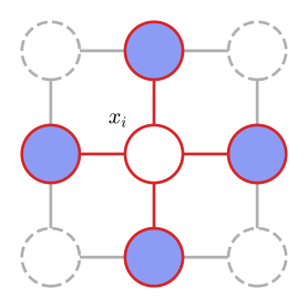
fig8_28. Download: PDF · SVG8.3.2 Factorization properties
pp. 384–387 Which factorisation goes with separation? If \(x_i\) and \(x_j\) are not linked, (8.38) must hold, so no factor may contain both. This leads to cliques.
Definition 8.5 (cliques and the Gibbs factorisation) pp. 385–386, (8.39)–(8.40)
A clique is a set of nodes in which every pair is linked; a maximal clique is a clique that cannot be enlarged by any other node. (In the book's Figure 8.29, with links \(x_1x_2\), \(x_2x_3\), \(x_3x_4\), \(x_4x_2\), \(x_1x_3\), the two-node cliques are those five pairs and the maximal cliques are \(\{x_1,x_2,x_3\}\) and \(\{x_2,x_3,x_4\}\); \(\{x_1,x_2,x_3,x_4\}\) is not a clique because \(x_1x_4\) is missing.) A distribution factorises over the graph if
\[ p(\mathbf{x})=\frac1Z\prod_{C}\psi_C(\mathbf{x}_C), \tag{8.39} \]a product over the maximal cliques \(C\) of nonnegative potential functions \(\psi_C\), with the partition function
\[ Z=\sum_{\mathbf{x}}\prod_{C}\psi_C(\mathbf{x}_C) \tag{8.40} \](integrals for continuous variables). The set of such distributions is the book's \(\mathcal{UF}\).
Restricting to maximal cliques loses nothing: a factor on a smaller clique can be multiplied into any maximal clique that contains it. The potentials need not be marginals or conditionals, which is why \(Z\) is needed (for a directed graph each factor is normalised and \(Z=1\) automatically). Computing \(Z\) for \(M\) discrete nodes with \(K\) states is a sum of \(K^M\) terms in the worst case. It is needed for learning the parameters of the potentials, but not for conditionals (a ratio of two marginals, in which \(Z\) cancels) nor for marginals of a few variables, which can be computed from the unnormalised product and normalised at the end (p. 386).
Result 8.12 (factorisation implies the global Markov property: \(\mathcal{UF}\subseteq\mathcal{UI}\)) p. 387
Suppose \(p(\mathbf{x})=\prod_s\phi_s(\mathbf{x}_{S_s})\), where every \(S_s\) is a clique (not necessarily maximal) of an undirected graph. If \(C\) separates \(A\) from \(B\), then \(A\indep B\given C\). No positivity is needed.
Proof
Let \(\widetilde A\) be the set of nodes outside \(C\) that can be reached from \(A\) by a path avoiding \(C\) (so \(A\subseteq\widetilde A\)), and \(\widetilde B\) the remaining nodes outside \(C\) (so \(B\subseteq\widetilde B\), by separation). There is no link between \(\widetilde A\) and \(\widetilde B\): such a link would make its endpoint in \(\widetilde B\) reachable from \(A\). A clique cannot contain a node of \(\widetilde A\) and a node of \(\widetilde B\), since these would have to be linked. So every factor is a function of \(\mathbf{x}_{\widetilde A\cup C}\) or of \(\mathbf{x}_{\widetilde B\cup C}\); grouping them, \(p\)
The converse needs strictly positive potentials, and then the two descriptions coincide (p. 387).
Result 8.13 (the Hammersley-Clifford theorem; Clifford, 1990) p. 387
Let \(p\) be a strictly positive distribution of \(\mathbf{x}=(x_1,\dots,x_M)\) (discrete, or a density that is positive everywhere on a product space) and \(G\) an undirected graph on \(\{1,\dots,M\}\). The following are equivalent:
(i) \(p\) factorises as (8.39) over the maximal cliques of \(G\) with strictly positive potentials;
(ii) \(p\) has the global Markov property; (iii) the local Markov property; (iv) the pairwise Markov property (8.38).
In the book's notation: among strictly positive distributions, \(\mathcal{UI}=\mathcal{UF}\).
Proof
(i)\(\Rightarrow\)(ii) is Result 8.12, and (ii)\(\Rightarrow\)(iii)\(\Rightarrow\)(iv) is Result 8.11. It remains to show (iv)\(\Rightarrow\)(i), the hard direction.
Möbius inversion. For functions \(\Phi,H\) on the subsets of a finite set \(V\): if \(H(S)\)
by the binomial theorem, and \((1-1)^n\) is 1 for \(n=0\) and 0 otherwise.
The canonical potentials. Fix a reference configuration \(\mathbf{x}^*\). For \(U\subseteq V\), let \((\mathbf{x}_U,\mathbf{x}^*_{V\setminus U})\) be the configuration that agrees with \(\mathbf{x}\) on \(U\) and with \(\mathbf{x}^*\) elsewhere, and define
\[ H_S(\mathbf{x}_S)=\sum_{U\subseteq S}(-1)^{|S\setminus U|}\ln p(\mathbf{x}_U,\mathbf{x}^*_{V\setminus U}), \]which is finite (positivity) and depends on \(\mathbf{x}\) only through \(\mathbf{x}_S\). Möbius inversion with \(S=V\) gives \(\ln p(\mathbf{x})\)
Only cliques survive. Let \(S\) contain two nodes \(i,j\) that are not linked. Group the subsets \(U\subseteq S\) in fours, \(W\), \(W\cup\{i\}\), \(W\cup\{j\}\), \(W\cup\{i,j\}\) with \(W\subseteq S\setminus\{i,j\}\); their signs are \(+,-,-,+\) times \((-1)^{|S\setminus W|}\). Writing \(\mathbf z\) for the common values of all variables other than \(x_i,x_j\) in these four configurations, each group contributes \((-1)^{|S\setminus W|}\) times
\[ \ln\frac{p(x_i,x_j,\mathbf z)\;p(x_i^*,x_j^*,\mathbf z)}{p(x_i,x_j^*,\mathbf z)\;p(x_i^*,x_j,\mathbf z)}=\ln\frac{p(x_i\given\mathbf z)p(x_j\given\mathbf z)\;p(x_i^*\given\mathbf z)p(x_j^*\given\mathbf z)}{p(x_i\given\mathbf z)p(x_j^*\given\mathbf z)\;p(x_i^*\given\mathbf z)p(x_j\given\mathbf z)}=0, \]using (8.38) in each term (the factors \(p(\mathbf z)\) cancel). Hence \(H_S\equiv0\) unless \(S\) is a clique (the empty set and single nodes count as cliques).
Assemble. \(p(\mathbf{x})\)
Filling the gap 8.8: without positivity the theorem fails pp. 386–387
The book restricts to strictly positive potentials "to make a precise relationship". Here is a distribution with zeros that satisfies every independence of a graph but does not factorise over it (Moussouris, 1974).
Derivation
Take the four-cycle \(x_1-x_2-x_3-x_4-x_1\) with binary variables, and let \(p\) be uniform on the eight configurations \(0000\), \(1000\), \(1100\), \(1110\), \(1111\), \(0111\), \(0011\), \(0001\) (written \(x_1x_2x_3x_4\)).
Markov. The separation statements of the four-cycle are \(x_1\indep x_3\given\{x_2,x_4\}\) and \(x_2\indep x_4\given\{x_1,x_3\}\). For each of the four values of the conditioning pair, the support contains at most two configurations, and in each case one of the two remaining variables is constant given the condition, so the conditional distribution is a product. (I checked both statements for all conditioning values by enumeration.)
Not a factorisation. Suppose \(p\propto\psi_{12}\psi_{23}\psi_{34}\psi_{41}\). From \(p(0000)\gt0\): \(\psi_{41}(x_4{=}0,x_1{=}0)\gt0\). From \(p(0111)\gt0\): \(\psi_{12}(0,1)\gt0\). From \(p(1110)\gt0\): \(\psi_{23}(1,1)\gt0\) and \(\psi_{34}(1,0)\gt0\). Then the configuration \(0110\) has all four factors positive, so \(p(0110)\gt0\), but \(0110\) is not in the support. The Möbius construction fails because \(\ln p\) is \(-\infty\) at some configurations. ∎
p. 387 Strictly positive potentials can be written as exponentials,
\[ \psi_C(\mathbf{x}_C)=\exp\{-E(\mathbf{x}_C)\}, \tag{8.41} \]where \(E(\mathbf{x}_C)\) is an energy function and \(p(\mathbf{x})\)
8.3.3 Illustration: Image de-noising
pp. 387–390 A binary image \(x_i\in\{-1,+1\}\), \(i=1,\dots,D\), is observed as \(y_i\in\{-1,+1\}\) after each pixel has been flipped independently with a small probability (Besag, 1974; Geman and Geman, 1984; Besag, 1986). Two kinds of knowledge help: \(y_i\) usually equals \(x_i\), and neighbouring \(x_i\) usually agree. The graph of the book's Figure 8.31 links each \(x_i\) to its observation \(y_i\) and to its four lattice neighbours; its cliques are pairs. Giving the pair \(\{x_i,y_i\}\) energy \(-\eta x_iy_i\), each neighbour pair \(\{x_i,x_j\}\) energy \(-\beta x_ix_j\) (\(\eta,\beta\gt0\)), and adding a bias \(hx_i\) per pixel gives the energy
\[ E(\mathbf{x},\mathbf{y})=h\sum_ix_i-\beta\sum_{\{i,j\}}x_ix_j-\eta\sum_ix_iy_i \tag{8.42} \](the middle sum over neighbouring pairs), and the joint distribution
\[ p(\mathbf{x},\mathbf{y})=\frac1Z\exp\{-E(\mathbf{x},\mathbf{y})\}. \tag{8.43} \]Clamping \(\mathbf y\) to the observed image defines \(p(\mathbf{x}\given\mathbf{y})\), an Ising model; we want a configuration \(\mathbf{x}\) of high (ideally maximal) posterior probability.
Filling the gap 8.9: (8.43) is an Ising prior with independent flip noise pp. 388–389
The book motivates the energy informally. In fact the joint model (8.43) is exactly "Ising prior on the clean image, each pixel flipped independently", and \(\eta\) fixes the flip rate.
Derivation
Only the last term of (8.42) involves \(\mathbf y\). Summing \(\exp\{-E\}\) over \(\mathbf y\in\{-1,1\}^D\):
\[ \sum_{\mathbf y}\exp\Big\{\eta\sum_ix_iy_i\Big\}=\prod_i\big(e^{\eta x_i}+e^{-\eta x_i}\big)=(2\cosh\eta)^D, \]which does not depend on \(\mathbf x\) (since \(x_i=\pm1\)). Hence the marginal of the clean image is the Ising model \(p(\mathbf x)\)
The pixels are flipped independently with probability \(\rho\). The book's \(\eta=2.1\) corresponds to \(\rho=1/(1+e^{4.2})\approx0.015\), whereas the actual flip rate of 10% would give \(\eta=\frac12\ln9\approx1.10\). So the values \(\beta=1\), \(\eta=2.1\) are best read as tuning parameters of a MAP estimate rather than as the true noise model; the demonstration lets you vary both. ∎
Result 8.14 (the ICM update is local and never increases the energy; Exercise 8.13) p. 389
With all other pixels fixed,
\[ E(x_j=+1)-E(x_j=-1)=2h-2\beta\sum_{i\in\mathrm{ne}(j)}x_i-2\eta\,y_j, \]which involves only the neighbours of \(j\) and \(y_j\). The ICM update sets \(x_j=+1\) if \(\beta\sum_{i\in\mathrm{ne}(j)}x_i+\eta y_j-h\gt0\), \(x_j=-1\) if it is negative, and leaves \(x_j\) unchanged on a tie. The energy never increases, ICM stops after finitely many updates, and it stops at a configuration that no single-pixel change can improve.
Proof
The terms of (8.42) that contain \(x_j\) are \(hx_j\), \(-\beta x_jx_i\) for \(i\in\mathrm{ne}(j)\) and \(-\eta x_jy_j\); all other terms are the same for both values of \(x_j\) and cancel in the difference. Each of the three terms changes by its coefficient times \(+1-(-1)=2\), giving the formula. Choosing the value with lower energy (keeping the current value on a tie) can only lower \(E\) or leave it unchanged, and it lowers \(E\) strictly whenever \(x_j\) changes. There are finitely many configurations, so there can only be finitely many changes; once a full sweep changes nothing, no single flip lowers the energy: a local minimum of \(E\) (local maximum of \(p(\mathbf x\given\mathbf y)\)) with respect to single-pixel moves. It need not be the global minimum. ∎
Algorithm 8.2 (iterated conditional modes, ICM; Kittler and Föglein, 1984; Besag, 1986) p. 389
- Initialise \(x_i=y_i\) for all \(i\).
- Visit the pixels (raster order or at random). At pixel \(j\), set \(x_j\)
\({}=\mathrm{sign}\big(\beta\sum_{i\in\mathrm{ne}(j)}x_i+\eta y_j-h\big)\), keeping \(x_j\) on a tie (Result 8.14). - Stop when a sweep through all pixels changes nothing.
With \(\beta=1\), \(\eta=2.1\), \(h=0\) (equal prior weight on both colours), ICM started from the noisy image gives the ICM restoration of Figure 8.30. With \(\beta=0\) the neighbours are disconnected and the most probable image is the noisy one (Exercise 8.14: with \(\beta=h=0\) the energy \(-\eta\sum_ix_iy_i\) is minimised term by term by \(x_i=y_i\)).
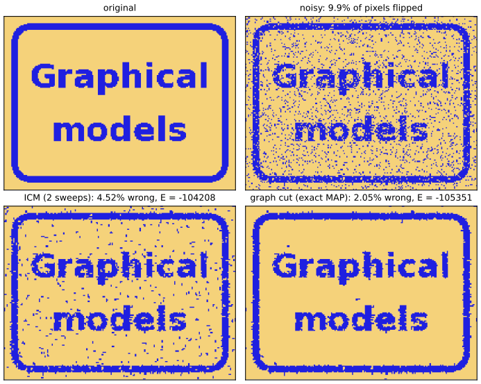
fig8_30. Download: PDF · SVGp. 390 The max-sum algorithm of Section 8.4.5 usually does better than ICM but is not exact on a lattice, which has loops. For this energy, however, the global maximum can be found exactly and efficiently by a minimum graph cut (Greig, Porteous and Seheult, 1989; Boykov, Veksler and Zabih, 2001; Kolmogorov and Zabih, 2004), as in the last panel of Figure 8.30.
Filling the gap 8.10: why a minimum cut gives the exact MAP image p. 390
The book only cites the graph-cut algorithms. The construction of Greig, Porteous and Seheult (1989) for binary images fits in a few lines.
Derivation
Rewrite the energy. Since \(x_ix_j=1-2[x_i\ne x_j]\) for \(\pm1\) values, (8.42) with \(\mathbf y\) fixed is
\[ E(\mathbf x)=\const+\sum_i\theta_i(x_i)+2\beta\sum_{\{i,j\}}[x_i\ne x_j],\qquad \theta_i(x_i)=hx_i-\eta x_iy_i . \]The network. Add a source \(s\) and a sink \(t\) to the pixel nodes. With \(m_i=\min\{\theta_i(+1),\theta_i(-1)\}\), give the link \(s\to i\) capacity \(a_i=\theta_i(-1)-m_i\ge0\), the link \(i\to t\) capacity \(c_i=\theta_i(+1)-m_i\ge0\), and for each neighbouring pair both links \(i\to j\) and \(j\to i\) capacity \(2\beta\ge0\). A cut splits the nodes into \(S\ni s\) and \(T\ni t\); its cost is the total capacity of the links from \(S\) to \(T\). Identify \(x_i=+1\) with \(i\in S\).
Cut cost = energy. A pixel with \(x_i=-1\) (in \(T\)) cuts \(s\to i\) and pays \(a_i\); one with \(x_i=+1\) cuts \(i\to t\) and pays \(c_i\); either way it pays \(\theta_i(x_i)-m_i\). A neighbouring pair with \(x_i\ne x_j\) has exactly one of its two links going from \(S\) to \(T\) and pays \(2\beta\); an agreeing pair pays nothing. So
\[ \text{cost}(S,T)=\sum_i\theta_i(x_i)+2\beta\sum_{\{i,j\}}[x_i\ne x_j]-\sum_im_i=E(\mathbf x)-\const' . \]Every configuration is a cut and vice versa, so a minimum cut is a minimum-energy (maximum posterior) image. By the max-flow min-cut theorem a minimum cut is found from a maximum flow in polynomial time. The construction needs nonnegative pair capacities, i.e. \(\beta\ge0\): energies that reward agreement (submodular energies; Kolmogorov and Zabih, 2004, characterise the binary energies that can be minimised this way). ∎
8.3.4 Relation to directed graphs
pp. 390–393 For the directed chain of Figure 8.32(a),
\[ p(\mathbf{x})=p(x_1)\,p(x_2\given x_1)\,p(x_3\given x_2)\cdots p(x_N\given x_{N-1}), \tag{8.44} \]and the undirected chain of Figure 8.32(b) has the maximal cliques \(\{x_{n-1},x_n\}\), so we want
\[ p(\mathbf{x})=\frac1Z\psi_{1,2}(x_1,x_2)\,\psi_{2,3}(x_2,x_3)\cdots\psi_{N-1,N}(x_{N-1},x_N). \tag{8.45} \]Take \(\psi_{1,2}(x_1,x_2)=p(x_1)p(x_2\given x_1)\) and \(\psi_{n-1,n}(x_{n-1},x_n)=p(x_n\given x_{n-1})\) for \(n\ge3\); then \(Z=1\).

fig8_32. Download: PDF · SVGIn general every conditional \(p(x_k\given\pa_k)\) must fit into some clique, so all parents of a node must be linked to each other. For the graph of Figure 8.33(a),
\[ p(\mathbf{x})=p(x_1)\,p(x_2)\,p(x_3)\,p(x_4\given x_1,x_2,x_3), \tag{8.46} \]the factor \(p(x_4\given x_1,x_2,x_3)\) requires the clique \(\{x_1,x_2,x_3,x_4\}\): "marrying the parents" (moralisation) produces the fully connected moral graph of Figure 8.33(b), which displays none of the independences of (8.46) (for example \(x_1\indep x_2\given\varnothing\)).
Algorithm 8.3 (from a directed to an undirected graph) pp. 391–392
- Moralise: for each node, link every pair of its parents; then drop all arrow heads.
- Set every maximal-clique potential of the moral graph to 1.
- Multiply each conditional \(p(x_k\given\pa_k)\) into one clique potential whose clique contains \(\{k\}\cup\pa_k\) (one exists because of step 1). Then \(Z=1\).
Result 8.15 (moralisation is correct and minimal) p. 392
Algorithm 8.3 represents every \(p\in\mathcal{DF}(G)\) as a factorisation (8.39) over the moral graph \(G^m\) with \(Z=1\); hence every independence read off \(G^m\) by separation holds for \(p\). The moral graph is the smallest such undirected graph: if an undirected graph \(U\) has the property that every \(p\in\mathcal{DF}(G)\) has the global Markov property for \(U\), then \(U\) contains all links of \(G^m\).
Proof
Correctness. \(\{k\}\cup\pa_k\) is a clique of \(G^m\) (\(k\) is linked to each parent, and the parents to each other), so it lies in some maximal clique. The product of the potentials is the product of all conditionals, which is \(p\) and sums to one, so \(Z=1\). Result 8.12 gives the global Markov property.
Minimality. Suppose \(U\) misses a link \(i-j\) of \(G^m\). In \(G\), either \(i\) and \(j\) are linked, or they are parents of a common child \(k\). In the first case they are never d-separated; in the second the path \(i\to k\leftarrow j\) is active given all other nodes (its head-to-head node \(k\) is observed). Either way \(i\) and \(j\) are not d-separated by the set of all other nodes, so by Result 8.9(c) some \(p\in\mathcal{DF}(G)\) has \(x_i\nindep x_j\given\mathbf x_{\setminus\{i,j\}}\). But \(i\) and \(j\) are not linked in \(U\), so the pairwise property of \(U\), which follows from its global property (Result 8.11), requires that independence. Contradiction. ∎
Moralisation is the first step of the junction tree algorithm (Section 8.4.6). Going from undirected to directed graphs is rarer and harder because of the normalisation constraints. To compare what the two kinds of graph can express, the book uses the filter view again.
Definition 8.6 (D map, I map, perfect map) p. 392
A graph is a D map (dependency map) of a distribution if every conditional independence satisfied by the distribution is reflected in the graph (by d-separation or separation); an I map (independence map) if every independence implied by the graph is satisfied by the distribution; and a perfect map if both. The graph without links is a trivial D map, and the fully connected graph a trivial I map, of every distribution.
Result 8.16 (each kind of graph expresses independences the other cannot) pp. 392–393, Figures 8.35, 8.36
(a) If the conditional independences of \(p(A,B,C)\) are exactly those of \(A\to C\leftarrow B\) (namely \(A\indep B\given\varnothing\) and nothing else, e.g. generic tables), no undirected graph on \(\{A,B,C\}\) is a perfect map of \(p\).
(b) If the conditional independences of \(p(A,B,C,D)\) are exactly those of the undirected four-cycle \(A-C-B-D-A\) (\(A\indep B\given\{C,D\}\), \(C\indep D\given\{A,B\}\), and nothing else; in particular \(A\nindep B\given\varnothing\)), no directed graph on these four variables is a perfect map of \(p\).
Proof
Adjacency. In a perfect map two nodes must be linked exactly when the distribution makes them dependent given every set of other variables. Undirected graphs: linked nodes are never separated, and non-linked nodes are separated by all the other nodes. Directed graphs: linked nodes are never d-separated, and if \(u\) precedes \(v\) in a topological order and they are not linked, \(\pa_v\) d-separates them (the claim in the proof of Result 8.9(b)).
(a) \(A\) and \(C\) are dependent given every subset of the other variables (nothing but \(A\indep B\) holds), and so are \(B\) and \(C\), so a perfect undirected map links \(A-C\) and \(B-C\). If it does not link \(A-B\), \(C\) separates them and the graph implies \(A\indep B\given C\), which \(p\) violates: not an I map. If it links \(A-B\), the graph is complete and shows no independence, but \(p\) has \(A\indep B\): not a D map.
(b) By the adjacency rule, a perfect DAG map has links exactly \(A-C\), \(C-B\), \(B-D\), \(D-A\). An acyclic orientation of a cycle cannot have all four links pointing the same way round, so at some node both cycle links point inwards. If this node is \(C\) (parents \(A\) and \(B\)), the path \(A\to C\leftarrow B\) is active given \(\{C,D\}\) (observed head-to-head node), so the DAG does not show \(A\indep B\given\{C,D\}\), which \(p\) satisfies: not a D map. If the node is \(D\), the same holds with \(D\) observed. If it is \(A\) or \(B\), the same argument applies to \(C\indep D\given\{A,B\}\). ∎
Graphs with both directed and undirected links (chain graphs; Lauritzen and Wermuth, 1989; Frydenberg, 1990) contain both classes, but there remain distributions without a perfect chain-graph map either (p. 393).
8.4 Inference in graphical models
pp. 393–394 Inference means computing the posterior distribution of some nodes when others are observed. The simplest case is Bayes' theorem itself (the book's Figure 8.37): with \(p(x,y)=p(x)p(y\given x)\) (graph \(x\to y\)) and \(y\) observed,
\[ p(y)=\sum_{x'}p(y\given x')\,p(x'), \tag{8.47} \] \[ p(x\given y)=\frac{p(y\given x)\,p(x)}{p(y)}, \tag{8.48} \]so the same joint is now written \(p(y)p(x\given y)\), the graph \(y\to x\) with the arrow reversed. The rest of the section turns this into algorithms that pass local messages along the links of a graph. They are exact on trees; Chapters 10 and 11 deal with approximate inference.
8.4.1 Inference on a chain
pp. 394–398 Take the undirected chain of Figure 8.32(b) (a directed chain gives the same graph, with \(Z=1\)):
\[ p(\mathbf{x})=\frac1Z\psi_{1,2}(x_1,x_2)\,\psi_{2,3}(x_2,x_3)\cdots\psi_{N-1,N}(x_{N-1},x_N), \tag{8.49} \]with \(N\) discrete nodes of \(K\) states, so each potential is a \(K\times K\) table and there are \((N-1)K^2\) numbers. The marginal of an interior node is
\[ p(x_n)=\sum_{x_1}\cdots\sum_{x_{n-1}}\sum_{x_{n+1}}\cdots\sum_{x_N}p(\mathbf{x}). \tag{8.50} \]Done naively this needs the \(K^N\) values of the joint. Instead, notice that only \(\psi_{N-1,N}\) contains \(x_N\), so
\[ \sum_{x_N}\psi_{N-1,N}(x_{N-1},x_N) \tag{8.51} \]can be done first, giving a function of \(x_{N-1}\), and so on from both ends:
\[ p(x_n)=\frac1Z\underbrace{\Bigg[\sum_{x_{n-1}}\psi_{n-1,n}(x_{n-1},x_n)\cdots\Big[\sum_{x_2}\psi_{2,3}(x_2,x_3)\Big[\sum_{x_1}\psi_{1,2}(x_1,x_2)\Big]\Big]\cdots\Bigg]}_{\mu_\alpha(x_n)}\;\underbrace{\Bigg[\sum_{x_{n+1}}\psi_{n,n+1}(x_n,x_{n+1})\cdots\Big[\sum_{x_N}\psi_{N-1,N}(x_{N-1},x_N)\Big]\cdots\Bigg]}_{\mu_\beta(x_n)}. \tag{8.52} \]The only fact used is the distributive law
\[ ab+ac=a(b+c), \tag{8.53} \]whose right side needs two operations instead of three. Hence
\[ p(x_n)=\frac1Z\,\mu_\alpha(x_n)\,\mu_\beta(x_n), \tag{8.54} \]where the forward and backward messages satisfy
\[ \mu_\alpha(x_n)=\sum_{x_{n-1}}\psi_{n-1,n}(x_{n-1},x_n)\Big[\sum_{x_{n-2}}\cdots\Big]=\sum_{x_{n-1}}\psi_{n-1,n}(x_{n-1},x_n)\,\mu_\alpha(x_{n-1}), \tag{8.55} \] \[ \mu_\alpha(x_2)=\sum_{x_1}\psi_{1,2}(x_1,x_2), \tag{8.56} \] \[ \mu_\beta(x_n)=\sum_{x_{n+1}}\psi_{n,n+1}(x_n,x_{n+1})\Big[\sum_{x_{n+2}}\cdots\Big]=\sum_{x_{n+1}}\psi_{n,n+1}(x_n,x_{n+1})\,\mu_\beta(x_{n+1}). \tag{8.57} \]Erratum. In some printings the indices and arguments of the potentials in (8.57) are ordered differently from (8.49) and the rest of the section; the form above, \(\psi_{n,n+1}(x_n,x_{n+1})\), is the corrected one.
Each message is a vector of \(K\) numbers and products of messages are taken elementwise. The outgoing message is the incoming one multiplied by the local potential and summed over the sending node's variable (the book's Figure 8.38). When the potentials come from a directed chain, these recursions are the Chapman-Kolmogorov equations of a Markov chain.
Result 8.17 (exact marginals on a chain in \(O(NK^2)\)) pp. 395–398, (8.49)–(8.58)
With \(\mu_\alpha(x_1)=1\) and \(\mu_\beta(x_N)=1\), the recursions (8.55) and (8.57) give (8.54) for every \(n\), with \(Z=\sum_{x_n}\mu_\alpha(x_n)\mu_\beta(x_n)\) for any \(n\), and the pairwise marginals
\[ p(x_{n-1},x_n)=\frac1Z\,\mu_\alpha(x_{n-1})\,\psi_{n-1,n}(x_{n-1},x_n)\,\mu_\beta(x_n). \tag{8.58} \]One marginal costs \(O(NK^2)\) operations; all \(N\) marginals together also cost \(O(NK^2)\) (one forward and one backward sweep, storing the messages), against \(O(N^2K^2)\) for \(N\) separate runs and \(O(NK^N)\) for brute force. Observed nodes are handled by restricting their sums to the observed value.
Proof
The messages. Define \(\mu_\alpha(x_n)\)
The marginal. In (8.50) the joint is \(\frac1Z\) times (left product, a function of \(x_1,\dots,x_n\)) times (right product, a function of \(x_n,\dots,x_N\)). With \(x_n\) fixed the two groups of summation variables are disjoint, so the sum of the product is the product of the sums (Result 8.19 below), which is (8.54). Summing (8.54) over \(x_n\) gives 1, hence \(Z=\sum_{x_n}\mu_\alpha\mu_\beta\), the same number at every \(n\). For (8.58) (Exercise 8.15) keep both \(x_{n-1}\) and \(x_n\) fixed: the joint splits into the left product up to \(x_{n-1}\), the single potential \(\psi_{n-1,n}\), and the right product from \(x_n\); summing the outer groups gives \(\mu_\alpha(x_{n-1})\psi_{n-1,n}\mu_\beta(x_n)/Z\).
Cost. One step of (8.55) computes \(K\) numbers, each a sum of \(K\) products: \(O(K^2)\). Reaching node \(n\) from both ends takes \(N-1\) steps: \(O(NK^2)\). Running the forward recursion from \(x_1\) to \(x_N\) and the backward one from \(x_N\) to \(x_1\) once, and storing all \(2(N-1)\) messages, gives every \(\mu_\alpha(x_n)\) and \(\mu_\beta(x_n)\), hence every marginal by (8.54) at \(O(K)\) extra cost each: \(O(NK^2)\) in total, twice the cost of one marginal. Repeating the single-marginal computation for each \(n\) would cost \(O(N^2K^2)\). Brute force evaluates \(K^N\) joint values of \(N-1\) factors each.
Directed chains. If \(\psi_{1,2}=p(x_1)p(x_2\given x_1)\) and \(\psi_{n-1,n}=p(x_n\given x_{n-1})\), then by induction \(\mu_\alpha(x_n)\)
Evidence. Observing \(x_m=\widehat x_m\) multiplies the joint by the indicator \(I(x_m,\widehat x_m)\), which can be absorbed into a potential containing \(x_m\). Every sum over \(x_m\) then has a single term. The recursions are unchanged, and the new normalising constant is \(Z\,p(\widehat x_m)\), so normalising (8.54) gives \(p(x_n\given\widehat x_m)\). ∎
Erratum. On p. 398 some printings give the cost of \(N\) separate runs as \(O(N^2M^2)\); it is \(O(N^2K^2)\).
The pairwise marginals (8.58) are exactly what the E step of EM needs when the potentials have parameters; Chapter 13 uses this for hidden Markov models (forward-backward algorithm). Exercises 8.16 and 8.17 treat an observed end node.
8.4.2 Trees
pp. 398–399 Message passing extends from chains to trees.
Definition 8.7 (trees and polytrees) p. 399, Figure 8.39
An undirected tree is a graph with exactly one path between every pair of nodes (connected and without loops). A directed tree has a single node without parents, the root, and every other node has exactly one parent. A polytree is a DAG with exactly one path (ignoring directions) between every pair of nodes, but in which some nodes have several parents.
Moralising a directed tree adds no links (no node has two parents), so it becomes an undirected tree; conversely an undirected tree can be directed away from any chosen root (Exercise 8.18). Moralising a polytree marries co-parents and creates loops; the factor graph of the next section keeps it a tree.
8.4.3 Factor graphs
pp. 399–402 Both kinds of graph express a product of factors; a factor graph (Frey, 1998; Kschischang, Frey and Loeliger, 2001) draws the factors themselves. Write
\[ p(\mathbf{x})=\prod_{s}f_s(\mathbf{x}_s), \tag{8.59} \]where each \(\mathbf{x}_s\) is a subset of the variables. The graph has a circle for each variable, a small square for each factor, and a link between \(f_s\) and every variable in \(\mathbf{x}_s\): it is bipartite (links only join nodes of opposite type). For example
\[ p(\mathbf{x})=f_a(x_1,x_2)\,f_b(x_1,x_2)\,f_c(x_2,x_3)\,f_d(x_3) \tag{8.60} \]is drawn in Figure 8.40. Directed graphs are the special case where the factors are the conditionals \(p(x_k\given\pa_k)\), undirected graphs the case where they are clique potentials (with \(1/Z\) as a factor on the empty set). A factor graph can say more: in (8.60) the two factors on \((x_1,x_2)\), which an undirected graph would merge into one clique potential, stay separate.
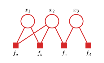
fig8_40. Download: PDF · SVGConversions (pp. 401–402). From an undirected graph: one factor node per maximal clique, with the clique potential as factor; other factor graphs give the same distribution if their factors multiply to the potentials (the book's Figure 8.41, whose caption should read \(f_b(x_2,x_3)\); see the errata). From a directed graph: one factor per conditional (Figure 8.42). A directed or undirected tree gives a tree factor graph; so does a polytree (Figure 8.43), and local cycles made by linked parents disappear inside a single factor (Figure 8.44). In the book's Figure 8.45, \(f_a(x_1,x_2)f_b(x_1,x_3)f_c(x_2,x_3)\) and \(f(x_1,x_2,x_3)\) have the same (complete) undirected graph, but the first restricts the distribution to pairwise interactions; it implies no conditional independence.
Filling the gap 8.11: the factor graph of a polytree is a tree p. 401, Figure 8.43
Derivation
Let the DAG have \(K\) nodes and \(E\) links, and build its factor graph with one factor per node \(k\), linked to \(k\) and to its parents. The factor graph has \(2K\) nodes and \(\sum_k(1+|\pa_k|)=K+E\) links, and it is connected exactly when the DAG's skeleton is (a factor joins a node to its parents). A connected graph is a tree if and only if it has one link fewer than nodes. So the factor graph is a tree iff \(K+E=2K-1\), i.e. \(E=K-1\), which for a connected skeleton on \(K\) nodes means that the skeleton is a tree: the DAG is a directed tree or a polytree. The moral graph of a polytree, by contrast, links co-parents that were already joined through their common child, closing a loop. ∎
8.4.4 The sum-product algorithm
pp. 402–411 From now on the factor graph is a tree (it came from an undirected tree, a directed tree or a polytree) and the variables are discrete; for continuous variables sums become integrals, and for linear-Gaussian models the messages are Gaussians (the Kalman filter, Chapter 13). Belief propagation for directed graphs without loops (Pearl, 1988; Lauritzen and Spiegelhalter, 1988, for junction trees) is a special case. The goal is the marginal of a variable \(x\),
\[ p(x)=\sum_{\mathbf{x}\setminus x}p(\mathbf{x}), \tag{8.61} \]and, with shared work, all the marginals at once. We assume first that nothing is observed and that \(p\) is normalised.
Result 8.18 (cutting a tree at a node) pp. 403–406, Figures 8.46–8.48
Remove a node \(v\) of a tree-structured factor graph. The remaining graph has exactly one component for each neighbour of \(v\), every other node lies in exactly one component, and every factor (other than \(v\) itself) involves only variables of its own component and possibly \(v\). Consequently, for a variable node \(x\),
\[ p(\mathbf{x})=\prod_{s\in\mathrm{ne}(x)}F_s(x,X_s), \tag{8.62} \]where \(X_s\) is the set of variables in the component containing the neighbouring factor \(f_s\) and \(F_s\) is the product of the factors in that component; the sets \(X_s\) are disjoint. In the same way, inside the component of \(f_s\), with \(\mathrm{ne}(f_s)=\{x,x_1,\dots,x_M\}\),
\[ F_s(x,X_s)=f_s(x,x_1,\dots,x_M)\,G_1(x_1,X_{s1})\cdots G_M(x_M,X_{sM}), \tag{8.65} \]and each \(G_m\) splits at \(x_m\) over the factors \(f_l\), \(l\in\mathrm{ne}(x_m)\setminus f_s\):
\[ G_m(x_m,X_{sm})=\prod_{l\in\mathrm{ne}(x_m)\setminus f_s}F_l(x_m,X_{lm}). \tag{8.68} \]Proof
Components. If two neighbours \(u,u'\) of \(v\) were joined by a path avoiding \(v\), adding \(u-v-u'\) would close a loop. So different neighbours lie in different components. Every other node \(w\) is joined to \(v\) by a unique path, and the last node before \(v\) on it is the neighbour whose component contains \(w\).
Factors stay in their component. The variables of a factor \(f\) are its neighbours in the factor graph, so they lie in the component of \(f\), or are \(v\) itself.
(8.62), (8.65), (8.68). Apply this with \(v=x\): the factors split into groups, one per neighbouring factor \(f_s\), and the group of \(f_s\) depends only on \(x\) and \(X_s\). Then apply it inside the component of \(f_s\) with \(v=f_s\): removing \(f_s\) leaves one sub-component per variable \(x_m\), whose factors multiply to \(G_m(x_m,X_{sm})\). Finally apply it inside the sub-component of \(x_m\) with \(v=x_m\). ∎
Result 8.19 (the generalised distributive law) pp. 396, 404, (8.53)
If \(X_1,\dots,X_m\) are disjoint sets of variables and \(g_s\) depends only on \(X_s\), then
\[ \sum_{X_1,\dots,X_m}\prod_{s=1}^{m}g_s(X_s)=\prod_{s=1}^{m}\sum_{X_s}g_s(X_s),\qquad \max_{X_1,\dots,X_m}\prod_{s=1}^{m}g_s(X_s)=\prod_{s=1}^{m}\max_{X_s}g_s(X_s)\ \text{ if all }g_s\ge0. \]Proof
Induction on \(m\). For \(m=2\), \(\sum_{X_1}\sum_{X_2}g_1(X_1)g_2(X_2)\)
Filling the gap 8.12: the message equations (8.63)–(8.71) pp. 403–407
The book derives the messages in prose with "interchanging the sums and products". Here every interchange is justified by Results 8.18 and 8.19.
Derivation
Marginal as a product of factor-to-variable messages. Substitute (8.62) into (8.61). With \(x\) fixed, the sum over \(\mathbf{x}\setminus x\) is a sum over the disjoint sets \(X_s\), and the \(s\)-th factor depends only on \(X_s\). By Result 8.19,
\[ p(x)=\prod_{s\in\mathrm{ne}(x)}\Big[\sum_{X_s}F_s(x,X_s)\Big]=\prod_{s\in\mathrm{ne}(x)}\mu_{f_s\to x}(x), \tag{8.63} \] \[ \mu_{f_s\to x}(x)\equiv\sum_{X_s}F_s(x,X_s). \tag{8.64} \]Factor-to-variable messages. Substitute (8.65) into (8.64). The set \(X_s\) consists of \(x_1,\dots,x_M\) and the disjoint sets \(X_{s1},\dots,X_{sM}\). With \(x,x_1,\dots,x_M\) fixed, Result 8.19 applies to the sums over the \(X_{sm}\):
\[ \mu_{f_s\to x}(x)=\sum_{x_1}\cdots\sum_{x_M}f_s(x,x_1,\dots,x_M)\prod_{m\in\mathrm{ne}(f_s)\setminus x}\Big[\sum_{X_{sm}}G_m(x_m,X_{sm})\Big]=\sum_{x_1}\cdots\sum_{x_M}f_s(x,x_1,\dots,x_M)\prod_{m\in\mathrm{ne}(f_s)\setminus x}\mu_{x_m\to f_s}(x_m), \tag{8.66} \] \[ \mu_{x_m\to f_s}(x_m)\equiv\sum_{X_{sm}}G_m(x_m,X_{sm}). \tag{8.67} \]Variable-to-factor messages. Substitute (8.68) into (8.67); the sets \(X_{lm}\) are disjoint, so by Result 8.19 and (8.64) applied to the subtree of \(f_l\),
\[ \mu_{x_m\to f_s}(x_m)=\prod_{l\in\mathrm{ne}(x_m)\setminus f_s}\Big[\sum_{X_{lm}}F_l(x_m,X_{lm})\Big]=\prod_{l\in\mathrm{ne}(x_m)\setminus f_s}\mu_{f_l\to x_m}(x_m). \tag{8.69} \]Leaves. If \(x\) is a leaf variable node whose only neighbour is \(f\), its subtree has no factors: \(G\) is an empty product and
\[ \mu_{x\to f}(x)=1. \tag{8.70} \]If \(f\) is a leaf factor node, it depends only on its single neighbour \(x\), so \(F=f(x)\) and there is nothing to sum:
\[ \mu_{f\to x}(x)=f(x). \tag{8.71} \]Both rules are also what (8.69) and (8.66) give with no incoming messages (empty products equal 1).
Errata. In some printings the first line after (8.65) has \(f_x\) for \(f_s\); the last sum inside the brackets in the first line of (8.66) is over \(X_{xm}\) instead of \(X_{sm}\); and \(X_{ml}\) appears instead of \(X_{lm}\) in (8.68)–(8.69) and Figure 8.48. The forms above are the corrected ones. ∎
In words: a factor node multiplies its factor by the incoming messages on all other links and sums out every variable except the recipient (8.66); a variable node multiplies the incoming messages on all other links (8.69), so a variable node with two neighbours just passes messages through. Every message is a function of the variable on its link. A node can send along a link once it has received messages on all its other links.
Algorithm 8.4 (the sum-product algorithm on a tree) pp. 406–408
- Pick any node (variable or factor) as the root.
- Inward pass. Leaves send (8.70) or (8.71). Every other node, once it has received messages from all neighbours except the one towards the root, sends its message towards the root with (8.66) or (8.69).
- Outward pass. The root, now holding messages from all its neighbours, sends to each of them; every node, on receiving the message from the root side, sends to all its other neighbours. Stop when a message has crossed every link in both directions.
- Marginals. \(p(x)=\prod_{s\in\mathrm{ne}(x)}\mu_{f_s\to x}(x)\) for every variable (8.63), and \(p(\mathbf{x}_s)\)
\({}=f_s(\mathbf{x}_s)\prod_{i\in\mathrm{ne}(f_s)}\mu_{x_i\to f_s}(x_i)\) for every factor (8.72).
Result 8.20 (sum-product is exact on trees; Exercise 8.20) pp. 406–408
On a tree-structured factor graph, the messages computed by (8.66), (8.69) from the leaf rules (8.70), (8.71) equal the subtree sums (8.64), (8.67), so (8.63) gives the exact marginal of every variable. The two-pass schedule of Algorithm 8.4 is always feasible (every node has the messages it needs when it must send), computes exactly two messages per link, and gives the same result whatever the root.
Proof
Sides of a link. Cutting the link between neighbours \(u\) and \(v\) splits the tree in two (Result 8.18); call the part containing \(u\) the side of the directed link \(u\to v\), and let \(d(u\to v)\) be its number of nodes. If \(w\ne v\) is another neighbour of \(u\), the side of \(w\to u\) is strictly contained in the side of \(u\to v\), so \(d(w\to u)\lt d(u\to v)\).
Exactness. By induction on \(d\). If \(d(u\to v)=1\), \(u\) is a leaf and its message (8.70) or (8.71) is the subtree sum by Filling the gap 8.12. Otherwise the message on \(u\to v\) is computed by (8.66) or (8.69) from the messages on the links \(w\to u\), \(w\ne v\), which have smaller sides and are exact by the induction hypothesis; the derivations of (8.66) and (8.69) then show that the result is the subtree sum (8.64) or (8.67) for the side of \(u\to v\). Every message, in particular each \(\mu_{f_s\to x}\) used in (8.63), is therefore exact, whatever the order in which messages were computed.
Feasibility. Send the messages in increasing order of \(d\). The messages needed for \(u\to v\) are those on links \(w\to u\) with smaller \(d\), already sent. The inward pass of Algorithm 8.4 sends every link pointing towards the root, the outward pass every link pointing away; within each pass a node sends only after receiving from all its other neighbours, which is a special case of this ordering argument. (The book's own induction, Exercise 8.20: a tree grows by adding leaves one at a time; a new leaf can send first in the inward pass and receive last in the outward pass, without disturbing the schedule of the smaller tree.)
Count and root. Each link carries one message each way, \(2\times\)(number of links) messages in total, the cost of about two single-marginal computations; running the single-marginal algorithm separately for each of \(n\) variables would cost of order \(n\) times more. By the exactness argument each message is determined by its link and direction alone, so the root plays no role. ∎
Cost. A message from a factor with \(M+1\) discrete variables of \(K\) states sums over \(K^M\) configurations for each of \(K\) values: \(O(K^{M+1})\), exponential in the size of the factor but not in the size of the graph. A message from a variable with \(d\) neighbours costs \(O(dK)\).
Result 8.21 (factor marginals and the message identity; Exercises 8.21, 8.23, 8.24) p. 408, (8.72)
On a tree, after both passes, for every factor
\[ p(\mathbf{x}_s)=f_s(\mathbf{x}_s)\prod_{i\in\mathrm{ne}(f_s)}\mu_{x_i\to f_s}(x_i), \tag{8.72} \]and for every variable \(x\) and neighbouring factor \(f_s\), \(p(x)=\mu_{f_s\to x}(x)\,\mu_{x\to f_s}(x)\).
Proof
(8.72). Cut the tree at \(f_s\) (Result 8.18): one component per neighbour \(x_i\), with factor product \(G_i(x_i,X_{si})\), and \(p(\mathbf x)\)
The identity. From (8.63) and (8.69), \(p(x)\)
Substituting (8.69) into (8.66) eliminates the variable-to-factor messages: each factor multiplies the messages from the factors beyond its variables, multiplies by its own factor and sums (the book's Figure 8.50).
Filling the gap 8.13: unnormalised models, evidence and rescaling pp. 408, 410
The book says that normalisation is "easily handled" and that observed variables are clamped. Here is why both work, and a third fact that every implementation uses.
Derivation
Unnormalised models. Every message is linear in each factor, so running the algorithm on \(\widetilde p(\mathbf x)=Z\,p(\mathbf x)\) (for instance with the clique potentials of an undirected graph and without \(1/Z\)) gives \(\widetilde p(x_i)=Z\,p(x_i)\) at every node. Then \(Z=\sum_{x_i}\widetilde p(x_i)\) can be computed at any single node at cost \(O(K)\), and must come out the same at all nodes (a useful check).
Evidence. Split \(\mathbf x\) into hidden \(\mathbf h\) and observed \(\mathbf v\) with values \(\widehat{\mathbf v}\). Multiply the joint by \(\prod_iI(v_i,\widehat v_i)\), attaching each indicator to a factor containing \(v_i\) (or as a new leaf factor). The product equals \(p(\mathbf h,\mathbf v=\widehat{\mathbf v})\), an unnormalised version of \(p(\mathbf h\given\widehat{\mathbf v})\) whose normalising constant is the evidence \(p(\widehat{\mathbf v})\). So one run gives every posterior marginal \(p(h_i\given\widehat{\mathbf v})\)
Rescaling. Multiplying any message by a positive constant multiplies every message computed from it, and hence some marginals, by the same constant, and does not change any normalised marginal (a marginal is a product of messages). So messages may be normalised to sum to one after every step, which prevents underflow on long chains; keeping the logarithms of the scale factors recovers \(\ln Z\). This is the scaling used for hidden Markov models in Chapter 13. ∎
A worked example pp. 408–410, (8.73)–(8.86), Figures 8.51, 8.52
The factor graph of Figure 8.51 has the unnormalised joint
\[ \widetilde p(\mathbf{x})=f_a(x_1,x_2)\,f_b(x_2,x_3)\,f_c(x_2,x_4). \tag{8.73} \]With \(x_3\) as root, \(x_1\) and \(x_4\) are leaves, and the inward pass sends
\[ \mu_{x_1\to f_a}(x_1)=1, \tag{8.74} \] \[ \mu_{f_a\to x_2}(x_2)=\sum_{x_1}f_a(x_1,x_2), \tag{8.75} \] \[ \mu_{x_4\to f_c}(x_4)=1, \tag{8.76} \] \[ \mu_{f_c\to x_2}(x_2)=\sum_{x_4}f_c(x_2,x_4), \tag{8.77} \] \[ \mu_{x_2\to f_b}(x_2)=\mu_{f_a\to x_2}(x_2)\,\mu_{f_c\to x_2}(x_2), \tag{8.78} \] \[ \mu_{f_b\to x_3}(x_3)=\sum_{x_2}f_b(x_2,x_3)\,\mu_{x_2\to f_b}(x_2); \tag{8.79} \]the outward pass sends
\[ \mu_{x_3\to f_b}(x_3)=1, \tag{8.80} \] \[ \mu_{f_b\to x_2}(x_2)=\sum_{x_3}f_b(x_2,x_3), \tag{8.81} \] \[ \mu_{x_2\to f_a}(x_2)=\mu_{f_b\to x_2}(x_2)\,\mu_{f_c\to x_2}(x_2), \tag{8.82} \] \[ \mu_{f_a\to x_1}(x_1)=\sum_{x_2}f_a(x_1,x_2)\,\mu_{x_2\to f_a}(x_2), \tag{8.83} \] \[ \mu_{x_2\to f_c}(x_2)=\mu_{f_a\to x_2}(x_2)\,\mu_{f_b\to x_2}(x_2), \tag{8.84} \] \[ \mu_{f_c\to x_4}(x_4)=\sum_{x_2}f_c(x_2,x_4)\,\mu_{x_2\to f_c}(x_2). \tag{8.85} \]Erratum. Some printings end (8.79) with "\(\mu_{x_2\to f_b}.\)" without the argument; it is \(\mu_{x_2\to f_b}(x_2)\).
The check on \(x_2\) is
\[ \widetilde p(x_2)=\mu_{f_a\to x_2}(x_2)\,\mu_{f_b\to x_2}(x_2)\,\mu_{f_c\to x_2}(x_2)=\Big[\sum_{x_1}f_a(x_1,x_2)\Big]\Big[\sum_{x_3}f_b(x_2,x_3)\Big]\Big[\sum_{x_4}f_c(x_2,x_4)\Big]=\sum_{x_1}\sum_{x_3}\sum_{x_4}\widetilde p(\mathbf{x}). \tag{8.86} \]Erratum. In some printings the middle summation of the second line of (8.86) runs over \(x_2\); it is over \(x_3\).
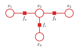
fig8_51. Download: PDF · SVG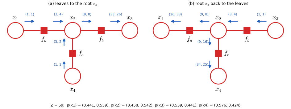
fig8_52. Download: PDF · SVGFilling the gap 8.14: the example with numbers, and with evidence pp. 409–410; Exercise 8.25
The book verifies (8.86) symbolically. Here the twelve messages are computed for actual tables, every marginal is compared with brute-force enumeration, and an observation is added.
Derivation
Let all variables be binary (states 0, 1) and take, with rows indexing the first argument,
\[ f_a=\begin{pmatrix}3&1\\1&2\end{pmatrix},\qquad f_b=\begin{pmatrix}2&1\\1&3\end{pmatrix},\qquad f_c=\begin{pmatrix}1&2\\3&1\end{pmatrix}. \]| message | formula | value at 0 | value at 1 |
|---|---|---|---|
| \(\mu_{f_a\to x_2}\) | column sums of \(f_a\) (8.75) | 4 | 3 |
| \(\mu_{f_c\to x_2}\) | row sums of \(f_c\) (8.77) | 3 | 4 |
| \(\mu_{x_2\to f_b}\) | product (8.78) | 12 | 12 |
| \(\mu_{f_b\to x_3}\) | (8.79) | \(3\cdot12=36\) | \(4\cdot12=48\) |
| \(\mu_{f_b\to x_2}\) | row sums of \(f_b\) (8.81) | 3 | 4 |
| \(\mu_{x_2\to f_a}\) | \(\mu_{f_b\to x_2}\mu_{f_c\to x_2}\) (8.82) | 9 | 16 |
| \(\mu_{f_a\to x_1}\) | \(3\cdot9+1\cdot16,\ 1\cdot9+2\cdot16\) (8.83) | 43 | 41 |
| \(\mu_{x_2\to f_c}\) | \(\mu_{f_a\to x_2}\mu_{f_b\to x_2}\) (8.84) | 12 | 12 |
| \(\mu_{f_c\to x_4}\) | (8.85) | \(4\cdot12=48\) | \(3\cdot12=36\) |
Marginals. \(\widetilde p(x_1)=\mu_{f_a\to x_1}=(43,41)\); \(\widetilde p(x_2)\)
A factor marginal (8.72), the last part of Exercise 8.25: \(\widetilde p(x_1,x_2)\)
Evidence. Observe \(x_3=1\). Clamping replaces \(\mu_{x_3\to f_b}=(1,1)\) by \((0,1)\), so \(\mu_{f_b\to x_2}=(f_b(0,1),f_b(1,1))=(1,3)\), and \(\widetilde p(x_2,x_3{=}1)\)
Nothing above used discreteness: for continuous variables the sums are integrals (p. 410), and for linear-Gaussian models every message is a Gaussian (Section 13.3).
8.4.5 The max-sum algorithm
pp. 411–415 Two other tasks are to find a configuration of highest probability and that probability:
\[ \mathbf{x}^{\max}=\argmax_{\mathbf{x}}p(\mathbf{x}), \tag{8.87} \] \[ p(\mathbf{x}^{\max})=\max_{\mathbf{x}}p(\mathbf{x}). \tag{8.88} \]Maximising each marginal separately answers a different question. In the book's Table 8.1, \(p(x,y)\) is 0.3 at \((0,0)\), 0.4 at \((1,0)\), 0.3 at \((0,1)\) and 0 at \((1,1)\). The joint is largest at \((1,0)\) (0.4), but the marginals \(p(x=0)=0.6\), \(p(y=0)=0.7\) pick \((0,0)\), whose joint probability is 0.3; Exercise 8.27 makes it 0. The same happens in the worked example above: the marginals pick \(x_1=0\), \(x_2=1\), \(x_3=1\), \(x_4=0\) with \(\widetilde p=9\), while the maximum is \(\widetilde p=18\) at \((1,1,1,0)\) (computed below).
To compute the maximum, write it as nested maximisations,
\[ \max_{\mathbf{x}}p(\mathbf{x})=\max_{x_1}\cdots\max_{x_M}p(\mathbf{x}), \tag{8.89} \]and use the distributive law for the maximum,
\[ \max(ab,ac)=a\max(b,c)\qquad(a\ge0), \tag{8.90} \]which holds because multiplying by \(a\ge0\) preserves order (for \(a\lt0\) it would reverse it; factors of graphical models are nonnegative). For the chain (8.49),
\[ \max_{\mathbf x}p(\mathbf x)=\frac1Z\max_{x_1}\cdots\max_{x_N}\big[\psi_{1,2}(x_1,x_2)\cdots\psi_{N-1,N}(x_{N-1},x_N)\big]=\frac1Z\max_{x_1}\Big[\max_{x_2}\Big[\psi_{1,2}(x_1,x_2)\Big[\cdots\max_{x_N}\psi_{N-1,N}(x_{N-1},x_N)\Big]\cdots\Big]\Big], \]a backward pass of messages from \(x_N\) to \(x_1\).
Erratum. In some printings the second line of this unnumbered display (p. 412) is misprinted; the corrected form, given in the errata, is the one above.
Products of many probabilities underflow, so one works with logarithms. The logarithm is increasing, so
\[ \ln\Big(\max_{\mathbf{x}}p(\mathbf{x})\Big)=\max_{\mathbf{x}}\ln p(\mathbf{x}), \tag{8.91} \]and the distributive law becomes
\[ \max(a+b,a+c)=a+\max(b,c), \tag{8.92} \]now with no sign condition. Replacing sums by maxima and products by sums of logarithms in (8.66), (8.69), (8.70), (8.71) and (8.63) gives the max-sum messages
\[ \mu_{f\to x}(x)=\max_{x_1,\dots,x_M}\Big[\ln f(x,x_1,\dots,x_M)+\sum_{m\in\mathrm{ne}(f)\setminus x}\mu_{x_m\to f}(x_m)\Big], \tag{8.93} \] \[ \mu_{x\to f}(x)=\sum_{l\in\mathrm{ne}(x)\setminus f}\mu_{f_l\to x}(x), \tag{8.94} \]with leaf messages
\[ \mu_{x\to f}(x)=0, \tag{8.95} \] \[ \mu_{f\to x}(x)=\ln f(x), \tag{8.96} \]and, at the root,
\[ p^{\max}=\max_{x}\Big[\sum_{s\in\mathrm{ne}(x)}\mu_{f_s\to x}(x)\Big], \tag{8.97} \] \[ x^{\max}=\argmax_{x}\Big[\sum_{s\in\mathrm{ne}(x)}\mu_{f_s\to x}(x)\Big]. \tag{8.98} \]Erratum. Some printings write \(\mathrm{ne}(f_s)\) under the sum in (8.93); it is \(\mathrm{ne}(f)\). Note also that (8.97) gives \(\ln p^{\max}\) (or \(\ln\) of the unnormalised maximum), not \(p^{\max}\) itself.
Filling the gap 8.15: why the max-sum messages are exact on a tree pp. 412–413, (8.89)–(8.98)
The book says the derivation is "identical" to sum-product. It is, once the distributive law is stated for maxima over disjoint sets.
Derivation
Replace \(\sum\) by \(\max\) everywhere in Filling the gap 8.12. With \(x\) fixed, \(\max_{\mathbf x\setminus x}\prod_sF_s(x,X_s)\)
Recovering the configuration. It is tempting to send max-sum messages back out from the root and apply (8.98) at every node. If the maximiser is unique this works: the max-marginal of \(x_i\) equals \(\max p\) at \(x_i^{\max}\) and is strictly smaller elsewhere. With ties it can fail: if \(p\) is uniform on \(\{(0,0),(1,1)\}\), both max-marginals are flat, and choosing each variable's maximiser independently may return \((0,1)\), of probability zero. The cure is to remember, during the inward pass, which arguments achieved each maximum, and to trace them back (pp. 413–415). For a chain with root \(x_N\), the inward messages are
\[ \mu_{x_n\to f_{n,n+1}}(x_n)=\mu_{f_{n-1,n}\to x_n}(x_n),\qquad \mu_{f_{n-1,n}\to x_n}(x_n)=\max_{x_{n-1}}\big[\ln f_{n-1,n}(x_{n-1},x_n)+\mu_{x_{n-1}\to f_{n-1,n}}(x_{n-1})\big], \]starting from
\[ \mu_{x_1\to f_{1,2}}(x_1)=0, \tag{8.99} \]then
\[ x_N^{\max}=\argmax_{x_N}\big[\mu_{f_{N-1,N}\to x_N}(x_N)\big], \tag{8.100} \] \[ \phi(x_n)=\argmax_{x_{n-1}}\big[\ln f_{n-1,n}(x_{n-1},x_n)+\mu_{x_{n-1}\to f_{n-1,n}}(x_{n-1})\big], \tag{8.101} \] \[ x_{n-1}^{\max}=\phi(x_n^{\max}). \tag{8.102} \]Erratum. In the unnumbered equation before (8.99) and in (8.101), some printings write \(\mu_{x_{n-1}\to f_{n-1,n}}(x_n)\); the argument is \(x_{n-1}\), as above.
Result 8.22 (back-tracking returns a global maximiser) pp. 414–415, (8.99)–(8.102), Figure 8.53
On a chain, the configuration obtained from (8.100) and repeated use of (8.102), with any choice among tied maximisers, attains \(\max_{\mathbf x}p(\mathbf x)\). The same holds on a tree when each factor-to-variable message (8.93) towards the root stores, for every value of its recipient, a maximising configuration of the factor's other variables, and these are read off outward from the root.
Proof
Write \(m_n(x_n)=\mu_{f_{n-1,n}\to x_n}(x_n)\) and \(m_1\equiv0\). By (8.92) and induction, \(m_n(x_n)\)
Algorithm 8.5 (max-sum with back-tracking) pp. 412–415
- Pick a root variable. Inward pass with (8.93)–(8.96); with each factor message store the maximising arguments (the functions \(\phi\)).
- At the root: \(\ln\widetilde p^{\max}\) by (8.97) and \(x^{\max}\) by (8.98).
- Outward, from the root to the leaves: set each factor's other variables to the stored maximisers for the value already chosen for the variable on the root side (8.102).
- Evidence: clamp observed variables (indicator factors) and maximise over the rest. On a hidden Markov model this is the Viterbi algorithm (Chapter 13).
Filling the gap 8.16: max-sum on the worked example, and why logarithms pp. 412–415
Derivation
The tables of Gap 8.14. Work with products (max-product) for readability; the logarithms of all numbers give the max-sum messages. Root \(x_3\). Inward: \(\max_{x_1}f_a(x_1,x_2)=(3,2)\) with maximisers \(x_1=(0,1)\); \(\max_{x_4}f_c(x_2,x_4)=(2,3)\) with maximisers \(x_4=(1,0)\); \(\mu_{x_2\to f_b}=(3\cdot2,\ 2\cdot3)=(6,6)\); \(\mu_{f_b\to x_3}(x_3)\)
Why logarithms. A chain of 1000 binary variables with factors around 0.1 has joint probabilities around \(10^{-1000}\), far below the smallest positive double-precision number (about \(5\times10^{-324}\)); every product underflows to 0 and all maxima tie. Its logarithm, about \(-2303\), is harmless. (Sum-product avoids underflow by rescaling instead, Gap 8.13; max-sum may simply add.) ∎
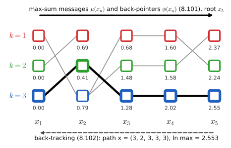
fig8_53. Download: PDF · SVGICM versus max-sum (p. 415). ICM passes a single value per update, max-sum a whole vector of \(K\) values per message. ICM is cheaper but may stop at a local optimum even on a tree; max-sum with back-tracking is exact on every tree.
8.4.6 Exact inference in general graphs
pp. 416–417 For graphs with loops the junction tree algorithm (Lauritzen and Spiegelhalter, 1988; Jordan, 2007) groups variables until the graph becomes a tree of clusters, and then runs sum-product on that tree.
Algorithm 8.6 (junction tree, in outline) p. 416
- Moralise a directed graph (Algorithm 8.3); an undirected graph is used as it is.
- Triangulate: add links until every cycle of four or more nodes has a chord (a link between two non-consecutive nodes of the cycle). The potentials are unchanged, merely regarded as functions of larger sets.
- Form the maximal cliques of the triangulated graph and join them into a junction tree: among all trees on the cliques, take one of maximum weight, the weight of a link being the number of variables the two cliques share.
- Assign each potential to one clique containing its variables and run two-pass message passing between cliques, summing out the variables that are not in the separator (the intersection of the two cliques). Each clique ends with the joint marginal of its variables.
Errata (p. 416). The text should read "A–C–B–D–A is chord-less and so a link should be added", "join tree" should be "junction tree", and the sentence beginning "If the tree is condensed" should be omitted.
Filling the gap 8.17: the junction tree on the four-cycle, and why triangulation is needed p. 416
The book describes the steps without an example. The four-cycle of Figure 8.36 shows every step and also what goes wrong without triangulation.
Derivation
Without triangulation. \(p(A,B,C,D)\)
With triangulation. Add the chord \(A-B\). The maximal cliques are \(\{A,B,C\}\) and \(\{A,B,D\}\) with separator \(\{A,B\}\). Put \(\Phi_1(A,B,C)=\psi_{AC}\psi_{CB}\) and \(\Phi_2(A,B,D)=\psi_{BD}\psi_{DA}\). The junction tree is the single link between the two cliques, and the two messages are
\[ m_{1\to2}(A,B)=\sum_C\Phi_1(A,B,C),\qquad m_{2\to1}(A,B)=\sum_D\Phi_2(A,B,D), \]giving \(p(A,B,D)=\Phi_2\,m_{1\to2}/Z\), \(p(A,B,C)=\Phi_1\,m_{2\to1}/Z\) and \(Z=\sum_{A,B}m_{1\to2}(A,B)\,m_{2\to1}(A,B)\). This is exactly sum-product on the chain factor graph \(C-\Phi_1-(A,B)-\Phi_2-D\) in which \((A,B)\) is treated as one variable with \(K^2\) states: the junction tree is a principled way of clustering variables so that the factor graph becomes a tree.
Cost. Messages between cliques cost of order \(K^{|\text{clique}|}\). The treewidth of a graph is one less than the size of the largest clique, minimised over all triangulations (Bodlaender, 1993); a tree has treewidth 1 and the four-cycle 2. The junction tree algorithm is exponential in the treewidth, and no general exact method can avoid this: exact inference in general discrete graphical models is NP-hard (Cooper, 1990). ∎
8.4.7 Loopy belief propagation
pp. 417–418 When exact inference is too expensive, one may simply run the local updates (8.66), (8.69) on a graph with loops: loopy belief propagation (Frey and MacKay, 1998). Every message is initialised to the unit function, so every node can send at once. A flooding schedule sends all messages simultaneously at each step; a serial schedule one at a time. Following Kschischang et al. (2001), a node \(a\) has a message pending on its link to \(b\) if \(a\) has received a message on another link since it last sent to \(b\); only pending messages need to be sent, because any other message would repeat the previous one. After stopping, approximate marginals are the products (8.63) and (8.72) of the latest messages.
Result 8.23 (pending messages; Exercises 8.28, 8.29) p. 418
(a) On a tree, any schedule that sends only pending messages (and sends one whenever one exists) stops after finitely many messages, and the final messages are the exact sum-product messages.
(b) On a factor graph with a cycle, there is always at least one pending message, however long the algorithm runs.
Proof
(a) Use the sides of links from Result 8.20 and induct on \(d(u\to v)\) to show that only finitely many messages are ever sent along \(u\to v\). If \(d(u\to v)=1\), \(u\) is a leaf with no other links, so after its first message it never receives anything that makes \(u\to v\) pending again. Otherwise, \(u\to v\) becomes pending only when \(u\) receives on some link \(w\to u\) with \(w\ne v\); by induction there are finitely many such receipts, and each makes at most one later message along \(u\to v\). Hence finitely many messages in total, and the schedule stops. When it stops nothing is pending, so the last message on each \(u\to v\) was computed after the last messages arrived on all the other links into \(u\), from those final messages. Induction on \(d\) again shows that the final messages are the exact ones (as in Result 8.20).
(b) Let \(n_1-n_2-\dots-n_k-n_1\) be a cycle, indices mod \(k\). Suppose that at some moment nothing is pending. Let \(s_i\) be the time at which \(n_i\) last sent to \(n_{i+1}\) (initial unit messages count as sent at time 0). Node \(n_i\) last received from \(n_{i-1}\) at time \(s_{i-1}\). Since \(n_i\) has nothing pending towards \(n_{i+1}\), it sent to \(n_{i+1}\) strictly after that receipt (a message sent in the same step could not use it): \(s_i\gt s_{i-1}\). Going round the cycle gives \(s_1\gt s_k\gt\dots\gt s_2\gt s_1\), a contradiction. ∎
So on loopy graphs one stops when the messages stop changing (or after a fixed number of steps). Convergence is not guaranteed, and the result is approximate even when it converges. Its fixed points are the stationary points of the Bethe free energy (Yedidia, Freeman and Weiss, 2005), and for a single loop the error can be analysed exactly (Weiss, 2000). Some state-of-the-art decoders of error-correcting codes are loopy belief propagation: turbo codes (Berrou et al., 1993; McEliece, MacKay and Cheng, 1998) and low-density parity-check codes (Gallager, 1962; MacKay and Neal, 1996; MacKay, 1999).
Filling the gap 8.18: how good is loopy belief propagation on a single loop? p. 418
The book says loopy belief propagation "can give poor results" in some applications and is "very effective" in others. A four-node example shows both regimes.
Derivation
Take \(x_1,\dots,x_4\in\{-1,+1\}\) on the cycle \(1-2-3-4-1\), with \(p(\mathbf x)\)
| coupling | method | \(p(x_1{=}1)\) | \(p(x_2{=}1)\) | \(p(x_3{=}1)\) | \(p(x_4{=}1)\) |
|---|---|---|---|---|---|
| \(J=0.5\) | exact | 0.615 | 0.505 | 0.557 | 0.565 |
| loopy BP | 0.625 | 0.506 | 0.562 | 0.571 | |
| \(J=1.5\) | exact | 0.599 | 0.596 | 0.597 | 0.598 |
| loopy BP | 0.857 | 0.844 | 0.850 | 0.852 |
With weak coupling the errors are below 0.01. With strong coupling loopy belief propagation is badly overconfident: each node's weak evidence travels round the loop and comes back reinforced, so it is counted many times. On a tree no message ever returns to its origin, which is why the same updates are exact there. ∎
8.4.8 Learning the graph structure
p. 418 So far the graph was given. To learn it from data (Friedman and Koller, 2003) we need a space of structures and a score. A Bayesian puts a prior \(p(m)\) on graphs \(m\) and uses
\[ p(m\given\mathcal D)\propto p(m)\,p(\mathcal D\given m), \tag{8.103} \]where the model evidence \(p(\mathcal D\given m)\) scores each structure; ideally predictions average over the posterior. Two difficulties: the evidence requires integrating over parameters (and latent variables), and the number of structures is enormous.
Filling the gap 8.19: the evidence of a discrete DAG in closed form p. 418, (8.103)
For complete discrete data and Dirichlet priors (the setting of Filling the gap 8.3) the evidence is a product of local terms (Cooper and Herskovits, 1992; Heckerman, Geiger and Chickering, 1995).
Derivation
The likelihood is \(\prod_{k,j}\prod_l\mu_{kjl}^{N_{kjl}}\), and the prior a product of independent \(\Dir(\bm\mu_{kj}\given\bm\alpha_{kj})\). The integral over all parameters factorises over the rows \((k,j)\), and each row is a Dirichlet integral: with \(\alpha_{kj}=\sum_l\alpha_{kjl}\), \(N_{kj}=\sum_lN_{kjl}\) and the Dirichlet normaliser \(\int\prod_l\mu_l^{a_l-1}\d\bm\mu\)
The logarithm is a sum of one term per node, depending only on that node and its parents: the score is decomposable, so adding or removing one link changes one or two terms, which makes local search over structures cheap. Choosing \(\alpha_{kjl}\) as an "equivalent sample size" times a prior guess of the joint (the BDe prior) gives the same evidence to all DAGs that encode the same independences. With latent variables the integral no longer factorises and needs the approximations of Chapters 9 to 11 (or the BIC). ∎
Result 8.24 (the number of DAGs grows super-exponentially; Robinson, 1973) p. 418
The number \(a(n)\) of DAGs on \(n\) labelled nodes satisfies \(a(0)=1\) and
\[ a(n)=\sum_{k=1}^{n}(-1)^{k+1}\binom nk\,2^{k(n-k)}\,a(n-k), \]giving \(1,3,25,543,29281,3781503,1138779265\) for \(n=1,\dots,7\). For comparison there are \(2^{n(n-1)/2}\) undirected graphs (Exercise 8.12): \(1,2,8,64,1024,32768,2097152\).
Proof
A source is a node without parents; every non-empty DAG has one (Result 8.1). Fix a set \(S\) of \(k\) nodes. The DAGs in which every node of \(S\) is a source are obtained, each exactly once, by choosing any DAG on the other \(n-k\) nodes (\(a(n-k)\) ways) and any set of links from \(S\) to the other nodes (\(2^{k(n-k)}\) ways); there are no links into \(S\), and links leaving sources cannot create cycles. By inclusion-exclusion over the set of sources, the number of DAGs with at least one source is \(\sum_{\varnothing\ne S}(-1)^{|S|+1}2^{|S|(n-|S|)}a(n-|S|)\), which is the formula after grouping the \(\binom nk\) sets of each size; and it equals \(a(n)\) since every DAG has a source. The values were computed from the recursion. Since \(a(n)\ge2^{n(n-1)/2}\) (every graph whose links all point from lower to higher labels is acyclic), \(\ln a(n)\) grows at least like \(n^2\). ∎
Exhaustive search is hopeless beyond a handful of nodes, and finding the highest-scoring DAG is NP-hard in general (Chickering, 1996); in practice one uses greedy local search, search over node orderings, or Markov chain Monte Carlo over structures (Friedman and Koller, 2003). Distinct DAGs can encode the same independences (for example \(a\to c\to b\), \(a\leftarrow c\leftarrow b\) and \(a\leftarrow c\to b\) all say exactly \(a\indep b\given c\)); data alone cannot distinguish them, and only the head-to-head structure \(a\to c\leftarrow b\) is identified.
Exercises
All 29 exercises of Chapter 8 (Bishop, 2006, pp. 418–422), restated in my own words, with complete solutions (hidden). Stars give the book's difficulty and "www" marks the exercises with official solutions. Several solutions are compact versions of the results above, which are linked for more detail.
Exercise 8.1 (★, www). By marginalising the variables in turn, show that (8.5) is normalised whenever each conditional distribution is.
Solution
Number the nodes topologically. The last node \(x_K\) has no children, so it appears only in \(p(x_K\given\pa_K)\), and \(\sum_{x_K}\prod_kp(x_k\given\pa_k)\)
\({}=\prod_{k\lt K}p(x_k\given\pa_k)\cdot\sum_{x_K}p(x_K\given\pa_K)\) \({}=\prod_{k\lt K}p(x_k\given\pa_k)\). The remaining product has the same form on \(K-1\) nodes. After \(K-1\) steps we are left with \(\sum_{x_1}p(x_1)=1\). Details, and why the factors are then the conditionals of the joint: Result 8.2. Exercise 8.2 (★, www). Show that if the nodes can be numbered so that no link goes to a lower-numbered node, the graph has no directed cycles.
Solution
Along a directed cycle \(k_1\to k_2\to\dots\to k_m\to k_1\) the numbers would strictly increase at every step and still return to \(k_1\): impossible. The converse (every DAG has such a numbering) is also proved in Result 8.1.
Exercise 8.3 (★★). For the joint distribution of Table 8.2 over binary \(a,b,c\), show that \(p(a,b)\ne p(a)p(b)\) but \(p(a,b\given c)=p(a\given c)p(b\given c)\) for \(c=0\) and \(c=1\).
Solution
Table 8.2: \(p(a,b,c)\) for \(abc=000,001,010,011,100,101,110,111\) is 0.192, 0.144, 0.048, 0.216, 0.192, 0.064, 0.048, 0.096.
Marginally dependent. \(p(a{=}0)=0.6\), \(p(b{=}0)\)
\({}=0.192+0.144+0.192+0.064\) \({}=0.592\), and \(p(a{=}0,b{=}0)=0.336\ne0.6\cdot0.592=0.3552\). Independent given \(c\). \(p(c{=}0)=0.48\): \(p(a,b\given c{=}0)\) is \(0.4,0.1,0.4,0.1\) for \(ab=00,01,10,11\), with \(p(a{=}0\given c{=}0)=0.5\) and \(p(b{=}0\given c{=}0)=0.8\); the products \(0.5\cdot0.8=0.4\), \(0.5\cdot0.2=0.1\), \(0.4\), \(0.1\) agree. \(p(c{=}1)=0.52\): \(p(a,b\given c{=}1)\) is \(\frac{0.144}{0.52},\frac{0.216}{0.52},\frac{0.064}{0.52},\frac{0.096}{0.52}\)
\({}=\frac{18}{65},\frac{27}{65},\frac{8}{65},\frac{12}{65}\), with \(p(a{=}0\given c{=}1)=\frac{9}{13}\) and \(p(b{=}0\given c{=}1)=0.4=\frac25\); the products \(\frac9{13}\cdot\frac25=\frac{18}{65}\), \(\frac9{13}\cdot\frac35=\frac{27}{65}\), \(\frac4{13}\cdot\frac25=\frac8{65}\), \(\frac4{13}\cdot\frac35=\frac{12}{65}\) agree. Exercise 8.4 (★★). For Table 8.2, compute \(p(a)\), \(p(b\given c)\) and \(p(c\given a)\), show that \(p(a,b,c)=p(a)p(c\given a)p(b\given c)\), and draw the graph.
Solution
\(p(a)=(0.6,0.4)\). \(p(c\given a)\): for \(a=0\), \(p(c{=}0)=(0.192+0.048)/0.6=0.4\), \(p(c{=}1)=0.6\); for \(a=1\), \(p(c{=}0)=(0.192+0.048)/0.4=0.6\), \(p(c{=}1)=0.4\). \(p(b\given c)\): for \(c=0\), \(p(b{=}0)=(0.192+0.192)/0.48=0.8\); for \(c=1\), \(p(b{=}0)=(0.144+0.064)/0.52=0.4\). Check all eight products, e.g. \(p(0,0,0)=0.6\cdot0.4\cdot0.8=0.192\), \(p(0,1,1)=0.6\cdot0.6\cdot0.6=0.216\), \(p(1,0,1)=0.4\cdot0.4\cdot0.4=0.064\), \(p(1,1,1)=0.4\cdot0.4\cdot0.6=0.096\) (all eight agree exactly). The graph is the head-to-tail chain \(a\to c\to b\), consistent with Exercise 8.3 (Result 8.7).
Exercise 8.5 (★, www). Draw the directed graphical model of the relevance vector machine, (7.79)–(7.80).
Solution
The model is \(p(\mathbf t\given\mathbf X,\mathbf w,\beta)\)
\({}=\prod_{n=1}^{N}\N(t_n\given\mathbf w^\T\bm\phi(\mathbf x_n),\beta^{-1})\) and \(p(\mathbf w\given\bm\alpha)\) \({}=\prod_{i=1}^{M}\N(w_i\given0,\alpha_i^{-1})\). (In some printings (7.79) has \(\beta^{-1}\) in the conditioning set; the parameter is \(\beta\). This does not affect the graph.) Each weight \(w_i\) has its own precision \(\alpha_i\) (plate over \(i\)); each target \(t_n\) depends on all weights, on its input \(\mathbf x_n\) and on \(\beta\) (plate over \(n\)); \(\mathbf x_n\), \(\alpha_i\) and \(\beta\) are parameters (solid dots) and \(t_n\) is observed. Exercise 8.5. The relevance vector machine as a directed graph with plates. Exercise 8.6 (★). The noisy-OR conditional (Pearl, 1988) is
\[ p(y=1\given x_1,\dots,x_M)=1-(1-\mu_0)\prod_{i=1}^{M}(1-\mu_i)^{x_i}, \tag{8.104} \]with \(0\le\mu_i\le1\) for \(i=0,\dots,M\). Show that it is a soft version of the logical OR, and discuss the interpretation of the \(\mu_i\).
Solution
A generative story. Let each active parent (\(x_i=1\)) independently switch \(y\) on with probability \(\mu_i\), and let a "leak" switch it on with probability \(\mu_0\) whatever the parents: \(z_0\sim\Bern(\mu_0)\), \(z_i\sim\Bern(\mu_ix_i)\), \(y=z_0\lor z_1\lor\dots\lor z_M\). Then \(y=0\) only if every \(z_i\) is 0, so \(p(y=0\given\mathbf x)\)
\({}=(1-\mu_0)\prod_i(1-\mu_ix_i)\) \({}=(1-\mu_0)\prod_i(1-\mu_i)^{x_i}\) (for \(x_i\in\{0,1\}\)), which is (8.104). Soft OR. With \(\mu_0=0\) and all \(\mu_i=1\), \(p(y=1\given\mathbf x)\) is 0 if all \(x_i=0\) and 1 otherwise: the logical OR. In general \(p(y=1)\) increases with every additional active parent, as for an OR, but no single parent is decisive.
Interpretation. \(\mu_i\) (\(i\ge1\)) is the probability that cause \(i\) on its own produces the effect, \(p(y=1\given x_i=1,\text{others }0)\) when \(\mu_0=0\); \(1-\mu_i\) is the probability that it is "inhibited". \(\mu_0\) is the probability of the effect when no listed cause is present (unmodelled causes). The table needs \(M+1\) parameters instead of \(2^M\), like (8.10) but with a different restriction: causes act independently through the probability of failure, so \(\ln p(y=0\given\mathbf x)\) is additive in the parents.
Exercise 8.7 (★★). Use (8.15) and (8.16) to derive the mean (8.17) and covariance (8.18) of the graph of Figure 8.14.
Solution
(8.15) gives \(\mu_1=b_1\), \(\mu_2=b_2+w_{21}b_1\), \(\mu_3=b_3+w_{32}\mu_2\). (8.16) for \(i\le j\), row by row: \(\Sigma_{11}=v_1\), \(\Sigma_{12}=w_{21}v_1\), \(\Sigma_{22}=w_{21}\Sigma_{12}+v_2\), \(\Sigma_{13}=w_{32}\Sigma_{12}\), \(\Sigma_{23}=w_{32}\Sigma_{22}\), \(\Sigma_{33}=w_{32}\Sigma_{23}+v_3\); the rest by symmetry. The full calculation, the warning that (8.16) holds only for \(i\le j\), and the precision matrix are in Filling the gap 8.5 and Result 8.5.
Exercise 8.8 (★, www). Show that \(a\indep b,c\given d\) implies \(a\indep b\given d\).
Solution
\(p(a,b,c\given d)=p(a\given d)p(b,c\given d)\) for every \(d\) with \(p(d)\gt0\). Summing over \(c\): \(p(a,b\given d)=p(a\given d)p(b\given d)\). See Result 8.6(b).
Exercise 8.9 (★, www). Use d-separation to show that a node is independent of all other nodes given its Markov blanket.
Solution
A path leaving \(x_i\) starts either through a parent (which is in the blanket and not head-to-head on the path: blocked), or through a child \(k\). If it continues from \(k\) to a child of \(k\), \(k\) is observed and head-to-tail: blocked. If it continues from \(k\) to another parent \(j\) of \(k\) (a co-parent, in the blanket), \(k\) is head-to-head and observed, so not blocked there, but \(j\) is observed and not head-to-head on the path (the link \(j\to k\) leaves \(j\) by its tail): blocked. So every path is blocked and Result 8.9 applies. Full version: Result 8.10.
Exercise 8.10 (★). In the graph of Figure 8.54 (\(a\to c\leftarrow b\), \(c\to d\)), show that \(a\indep b\given\varnothing\), and that in general \(a\nindep b\given d\).
Solution
Summing \(p(a)p(b)p(c\given a,b)p(d\given c)\) over \(d\) and then \(c\) gives \(p(a)p(b)\). Given \(d\), \(p(a,b\given d)\)
\({}\propto p(a)p(b)\sum_cp(c\given a,b)p(d\given c)\), which need not factorise; with \(c=a\oplus b\) and \(d\) a 90%-reliable copy of \(c\), \(p(a=1,b=1\given d=0)\) \({}=0.45\) \({}\ne0.25\) \({}=p(a=1\given d=0)p(b=1\given d=0)\). See Result 8.8. Exercise 8.11 (★★). In the fuel system of Figure 8.21, a driver reads the gauge and reports \(D\), with
\[ p(D=1\given G=1)=0.9, \tag{8.105} \] \[ p(D=0\given G=0)=0.9. \tag{8.106} \]Given the report \(D=0\), find the probability that the tank is empty; then add the observation \(B=0\). Explain, and relate to Figure 8.54.
Solution
From Filling the gap 8.6, \(p(G=0)=0.315\) and \(p(G=0\given F=0)=0.81\). Sum over \(G\): \(p(D=0)=0.9\cdot0.315+0.1\cdot0.685=0.352\), \(p(D=0\given F=0)\)
\[ p(F=0\given D=0)=\frac{0.748\cdot0.1}{0.352}=\frac{17}{80}=0.2125. \]\({}=0.9\cdot0.81+0.1\cdot0.19\) \({}=0.748\), so With the battery flat: \(p(D=0\given B=0,F=0)\)
\[ p(F=0\given D=0,B=0)=\frac{0.82\cdot0.1}{0.82\cdot0.1+0.74\cdot0.9}=\frac{0.082}{0.748}=\frac{41}{374}\approx0.110. \]\({}=0.9\cdot0.9+0.1\cdot0.1\) \({}=0.82\) and \(p(D=0\given B=0,F=1)\) \({}=0.9\cdot0.8+0.1\cdot0.2\) \({}=0.74\); as in (8.33) \(p(B=0)\) cancels and The second value is lower: the flat battery explains away the "empty" report. This is Figure 8.54 with \(a=B\), \(b=F\), \(c=G\), \(d=D\): observing a descendant of the head-to-head node \(G\) makes \(B\) and \(F\) dependent (Result 8.8). Both probabilities are closer to the prior 0.1 than the values 0.257 and 0.111 obtained from the gauge itself, because the report is a noisy version of the gauge. (Exact rational arithmetic.)
Exercise 8.12 (★, www). Show that there are \(2^{M(M-1)/2}\) distinct undirected graphs on \(M\) labelled nodes, and draw the 8 for \(M=3\).
Solution
A graph is determined by which of the \(\binom M2=M(M-1)/2\) possible links are present (each unordered pair counted once), and each can be present or absent independently: \(2^{M(M-1)/2}\) graphs. For \(M=3\), with nodes \(1,2,3\): the empty graph; three graphs with one link (\(1-2\), \(1-3\) or \(2-3\)); three paths with two links (centred at 1, 2 or 3); and the triangle. Compare the number of DAGs in Result 8.24 (25 for \(M=3\)).
Exercise 8.13 (★). For ICM on the energy (8.42), write the energy difference between the two states of \(x_j\) with all other variables fixed, and show that it depends only on quantities local to \(x_j\).
Solution
Only \(hx_j\), \(-\beta x_j\sum_{i\in\mathrm{ne}(j)}x_i\) and \(-\eta x_jy_j\) involve \(x_j\), so \(E(x_j{=}{+}1)-E(x_j{=}{-}1)\)
\({}=2h-2\beta\sum_{i\in\mathrm{ne}(j)}x_i-2\eta y_j\): it involves only the lattice neighbours of \(j\) and \(y_j\), i.e. the Markov blanket of \(x_j\). See Result 8.14. ▶ See it in a demo: ICM sweeps and the energy trace
Exercise 8.14 (★). With \(\beta=h=0\) in (8.42), show that the most probable \(\mathbf x\) is \(\mathbf x=\mathbf y\).
Solution
Then \(E=-\eta\sum_ix_iy_i\) is a sum of terms each involving one \(x_i\), so it is minimised term by term: \(-\eta x_iy_i\) is \(-\eta\) for \(x_i=y_i\) and \(+\eta\) otherwise, and \(\eta\gt0\). Hence \(x_i=y_i\) for all \(i\) is the unique minimiser of the energy, i.e. the unique maximiser of \(p(\mathbf x\given\mathbf y)\propto e^{-E}\). Without coupling, each pixel only sees its own observation.
▶ See it in a demo: no coupling, nothing restored
Exercise 8.15 (★★, www). Show that the joint distribution of two neighbouring nodes of the chain of Figure 8.38 is (8.58).
Solution
Sum the joint (8.49) over all variables except \(x_{n-1},x_n\). With these two fixed, the product splits into the potentials left of \(x_{n-1}\), the single potential \(\psi_{n-1,n}(x_{n-1},x_n)\), and the potentials right of \(x_n\); the left group involves the summation variables \(x_1,\dots,x_{n-2}\) only, the right group \(x_{n+1},\dots,x_N\) only. The sum of the product is the product of the sums (Result 8.19): \(\mu_\alpha(x_{n-1})\,\psi_{n-1,n}(x_{n-1},x_n)\,\mu_\beta(x_n)/Z\). See Result 8.17.
Exercise 8.16 (★★). Show how the chain algorithm of Section 8.4.1 computes \(p(x_n\given\widehat x_N)\) for all \(n\lt N\), and which messages change.
Solution
Clamp \(x_N=\widehat x_N\) by multiplying \(\psi_{N-1,N}\) by \(I(x_N,\widehat x_N)\). The forward messages \(\mu_\alpha(x_n)\), \(n\le N-1\), do not involve \(x_N\) and are unchanged. Every backward message changes: it starts from \(\mu_\beta(x_{N-1})\)
\({}=\psi_{N-1,N}(x_{N-1},\widehat x_N)\) (the sum over \(x_N\) has one term) and then follows (8.57). Then \(p(x_n\given\widehat x_N)\) \({}=\mu_\alpha(x_n)\mu_\beta(x_n)/Z'\) with \(Z'\) \({}=\sum_{x_n}\mu_\alpha(x_n)\mu_\beta(x_n)\) \({}=Z\,p(\widehat x_N)\), the same for every \(n\). Cost: one new backward sweep, \(O(NK^2)\). For a directed chain the new backward messages are \(\mu_\beta(x_n)=p(\widehat x_N\given x_n)\) (Chapman-Kolmogorov backwards), so the formula is Bayes' theorem \(p(x_n\given\widehat x_N)\) \({}\propto p(x_n)p(\widehat x_N\given x_n)\). ▶ See it in a demo: observed variables and normalisation
Exercise 8.17 (★★). In the chain of Figure 8.38 with \(N=5\) and \(x_3,x_5\) observed, show by d-separation that \(x_2\indep x_5\given x_3\), and that the message-passing value of \(p(x_2\given x_3,x_5)\) does not depend on \(x_5\).
Solution
Separation. The only path from \(x_2\) to \(x_5\) passes through \(x_3\), which is observed (head-to-tail in the directed chain; any observed node blocks a path in the undirected chain). So \(x_2\indep x_5\given x_3\).
Messages. With \(x_3,x_5\) clamped, \(\mu_\beta(x_4)=\psi_{4,5}(x_4,\widehat x_5)\), \(\mu_\beta(x_3)\)
\[ p(x_2\given\widehat x_3,\widehat x_5)=\frac{\mu_\alpha(x_2)\,\psi_{2,3}(x_2,\widehat x_3)\,c}{\sum_{x_2'}\mu_\alpha(x_2')\,\psi_{2,3}(x_2',\widehat x_3)\,c}, \]\({}=\sum_{x_4}\psi_{3,4}(x_3,x_4)\mu_\beta(x_4)\), evaluated only at \(x_3=\widehat x_3\), and \(\mu_\beta(x_2)\) \({}=\sum_{x_3}\psi_{2,3}(x_2,x_3)I(x_3,\widehat x_3)\mu_\beta(x_3)\) \({}=\psi_{2,3}(x_2,\widehat x_3)\,c(\widehat x_3,\widehat x_5)\), where the scalar \(c=\mu_\beta(\widehat x_3)\) is the only place \(\widehat x_5\) enters. Hence and \(c\) cancels.
Exercise 8.18 (★★, www). Show that a directed-tree distribution can be written over the corresponding undirected tree, and that an undirected-tree distribution can be written, by normalising the potentials, as a directed tree. How many directed trees correspond to one undirected tree?
Solution
Directed to undirected. Each non-root node has one parent, so (8.5) is \(p(x_r)\prod_{k\ne r}p(x_k\given x_{\pa(k)})\), a product of functions of linked pairs. Take \(\psi_{\pa(k),k}=p(x_k\given x_{\pa(k)})\) and multiply \(p(x_r)\) into one potential containing the root, exactly as in (8.44)–(8.45). Then \(Z=1\). Moralisation adds nothing (no co-parents).
Undirected to directed. Let \(p\propto\prod_{\text{links}}\psi_{ij}\), pick a root \(r\) and direct every link away from it. Remove leaves one at a time: for a leaf \(l\) with neighbour \(u\), set \(p(x_l\given x_u)=\psi_{ul}(x_u,x_l)/m(x_u)\) with \(m(x_u)=\sum_{x_l}\psi_{ul}(x_u,x_l)\), and multiply \(m(x_u)\) into another potential containing \(u\) (or keep it as a factor on \(u\) alone). The product is unchanged. When only \(r\) is left, its remaining factor, normalised, is \(p(x_r)\), and its normaliser is \(Z\). Now \(p=p(x_r)\prod_kp(x_k\given x_{\pa(k)})\), and these are the true conditionals by Result 8.2. (This is the inward pass of sum-product towards \(r\). If some \(m(x_u)=0\), that value of \(x_u\) has probability zero and \(p(x_l\given x_u)\) may be chosen arbitrarily.)
Counting. In a directed tree the path from the root to any node follows the arrows (go back through the unique parents; this must end at the root), so the root determines every orientation. Each of the \(N\) nodes can be the root: \(N\) directed trees, all representing the same family of distributions.
Exercise 8.19 (★★). Apply the sum-product algorithm to the chain of Section 8.4.1 and recover (8.54), (8.55) and (8.57).
Solution
The factor graph of (8.49) has factors \(f_{n-1,n}=\psi_{n-1,n}\) (put \(1/Z\) aside) and variable nodes with two neighbours (one for the end nodes). The leaf \(x_1\) sends \(\mu_{x_1\to f_{1,2}}=1\) (8.70). A variable with two neighbours forwards what it receives (8.69): \(\mu_{x_{n-1}\to f_{n-1,n}}\)
\[ \mu_{f_{n-1,n}\to x_n}(x_n)=\sum_{x_{n-1}}\psi_{n-1,n}(x_{n-1},x_n)\,\mu_{f_{n-2,n-1}\to x_{n-1}}(x_{n-1}). \]\({}=\mu_{f_{n-2,n-1}\to x_{n-1}}\). By (8.66), Writing \(\mu_\alpha(x_n)=\mu_{f_{n-1,n}\to x_n}(x_n)\) this is (8.55), and for \(n=2\) it is (8.56). In the same way \(\mu_\beta(x_n)=\mu_{f_{n,n+1}\to x_n}(x_n)\) satisfies (8.57) starting from \(\mu_{x_N\to f_{N-1,N}}=1\). Node \(x_n\) has the two neighbours \(f_{n-1,n}\), \(f_{n,n+1}\), so (8.63) gives \(\widetilde p(x_n)=\mu_\alpha(x_n)\mu_\beta(x_n)\), which is (8.54) after normalising.
▶ See it in a demo: forward and backward messages on a chain
Exercise 8.20 (★, www). Show by induction that, on a tree, the messages can be ordered (leaves to root, then root to leaves) so that every node has all the incoming messages it needs when it sends.
Solution
Induction on the number of nodes. A single node sends nothing. A tree with \(n+1\) nodes is a tree with \(n\) nodes plus a leaf \(l\) attached to a node \(u\) (remove any leaf). Inward pass: let \(l\) send first (it needs nothing), then follow the schedule of the smaller tree, in which \(u\) now also has \(l\)'s message before it sends towards the root. Outward pass: follow the smaller tree's schedule; when \(u\) has received from the root side it has everything needed to send to \(l\) last. A shorter argument orders the messages by the size of the sender's side of the link (Result 8.20).
Exercise 8.21 (★★, www). Show that the marginal over the variables \(\mathbf x_s\) of a factor \(f_s(\mathbf x_s)\) can be found after sum-product by (8.72).
Solution
Cut the tree at \(f_s\): \(p(\mathbf x)\)
\({}=f_s(\mathbf x_s)\prod_{i\in\mathrm{ne}(f_s)}G_i(x_i,X_{si})\) with disjoint \(X_{si}\) (Result 8.18). Summing over all variables not in \(\mathbf x_s\), the sum of the product is the product of the sums (Result 8.19), and \(\sum_{X_{si}}G_i=\mu_{x_i\to f_s}(x_i)\) by (8.67); after both passes of sum-product all these messages are available. Hence (8.72). (Erratum: the exercise should refer to \(f_s(\mathbf x_s)\), not \(f_x(\mathbf x_s)\).) See Result 8.21. Exercise 8.22 (★). In a tree-structured factor graph, let a subset \(S\) of the variables be connected through factor nodes. Show how to use sum-product to compute \(p(\mathbf x_S)\).
Solution
Let \(\mathcal F_S\) be the factors linked to at least two variables of \(S\). The nodes \(S\cup\mathcal F_S\) form a subtree (connected by assumption, loop-free because the whole graph is a tree). Cut every link leaving this subtree; each cut link leads into its own component (Result 8.18). Two kinds of cut link occur: \(x\in S\) to a factor \(g\notin\mathcal F_S\), whose component sums to \(\mu_{g\to x}(x)\); and \(f\in\mathcal F_S\) to a variable \(y\notin S\), whose component sums to \(\mu_{y\to f}(y)\). Each such \(y\) belongs to a single factor of the subtree, so its sum can be done locally:
\[ p(\mathbf x_S)\propto\prod_{f\in\mathcal F_S}\Big[\sum_{\mathbf y_f}f(\mathbf x_f)\prod_{y\in\mathrm{ne}(f)\setminus S}\mu_{y\to f}(y)\Big]\prod_{x\in S}\ \prod_{g\in\mathrm{ne}(x)\setminus\mathcal F_S}\mu_{g\to x}(x), \]where \(\mathbf y_f\) are the variables of \(f\) outside \(S\). All messages come from one standard two-pass run; normalise at the end. For \(S=\{x\}\) this is (8.63), and for \(S=\mathbf x_s\) it is (8.72).
Exercise 8.23 (★★, www). Show that \(p(x_i)\) equals the product of the incoming and outgoing messages on any one link at \(x_i\).
Solution
By (8.63) and (8.69), \(p(x_i)\)
\({}=\mu_{f_s\to x_i}(x_i)\prod_{t\in\mathrm{ne}(x_i)\setminus f_s}\mu_{f_t\to x_i}(x_i)\) \({}=\mu_{f_s\to x_i}(x_i)\,\mu_{x_i\to f_s}(x_i)\) for any \(f_s\in\mathrm{ne}(x_i)\). See Result 8.21. Exercise 8.24 (★★). Show that, after sum-product on a tree, the marginal of the variables of a factor is (8.72).
Solution
This is Exercise 8.21 again. Another way to see it: the messages \(\mu_{x_i\to f_s}\) arriving at \(f_s\) are, by (8.67), the sums over everything beyond \(x_i\); the factor \(f_s\) is the only remaining piece of the joint. Multiplying them and not summing anything gives the joint of \(\mathbf x_s\) with everything else summed out. Numerical check on Figure 8.51: Filling the gap 8.14.
Exercise 8.25 (★★). For the graph of Figure 8.51 with root \(x_3\), check that the marginals of \(x_1\) and \(x_3\) are correct, and that (8.72) gives the correct \(p(x_1,x_2)\).
Solution
Using (8.83), (8.82), (8.81), (8.77):
\[ \widetilde p(x_1)=\mu_{f_a\to x_1}(x_1)=\sum_{x_2}f_a(x_1,x_2)\,\mu_{f_b\to x_2}(x_2)\,\mu_{f_c\to x_2}(x_2)=\sum_{x_2}f_a(x_1,x_2)\sum_{x_3}f_b(x_2,x_3)\sum_{x_4}f_c(x_2,x_4)=\sum_{x_2,x_3,x_4}\widetilde p(\mathbf x). \]Using (8.79), (8.78), (8.75), (8.77):
\[ \widetilde p(x_3)=\mu_{f_b\to x_3}(x_3)=\sum_{x_2}f_b(x_2,x_3)\,\mu_{f_a\to x_2}(x_2)\,\mu_{f_c\to x_2}(x_2)=\sum_{x_2}f_b(x_2,x_3)\sum_{x_1}f_a(x_1,x_2)\sum_{x_4}f_c(x_2,x_4)=\sum_{x_1,x_2,x_4}\widetilde p(\mathbf x). \]And by (8.72), with (8.74) and (8.82):
\[ f_a(x_1,x_2)\,\mu_{x_1\to f_a}(x_1)\,\mu_{x_2\to f_a}(x_2)=f_a(x_1,x_2)\cdot1\cdot\sum_{x_3}f_b(x_2,x_3)\sum_{x_4}f_c(x_2,x_4)=\sum_{x_3,x_4}\widetilde p(\mathbf x). \]With numbers: Filling the gap 8.14 (\(\widetilde p(x_1)=(43,41)\), \(\widetilde p(x_3)=(36,48)\), \(\widetilde p(x_1,x_2)\) as computed there, all matching enumeration).
▶ See it in a demo: sum-product on Figure 8.51
Exercise 8.26 (★). Describe how to obtain \(p(x_a,x_b)\) for two variables that share no factor, by clamping one of them in turn to each of its values.
Solution
For each value \(k\) of \(x_a\): clamp \(x_a=k\) (an indicator factor), run sum-product, and read off the unnormalised marginal at \(x_b\), which is \(\widetilde p(x_b,x_a=k)=Z\,p(x_a=k,x_b)\) (Filling the gap 8.13). Doing this for all \(K_a\) values gives the whole table up to the constant \(Z\), which is its total sum (or comes from an unclamped run). Only the messages on the path from \(x_a\) towards \(x_b\) change with \(k\), so each extra run costs only that path. Equivalently, \(p(x_a,x_b)=p(x_a)\,p(x_b\given x_a)\), with \(p(x_b\given x_a=k)\) from the clamped run.
Exercise 8.27 (★★). Construct \(p(x,y)\) on \(\{0,1,2\}^2\) such that the maximisers \(\widehat x\) of \(p(x)\) and \(\widehat y\) of \(p(y)\) satisfy \(p(\widehat x,\widehat y)=0\).
Solution
Take (rows \(x=0,1,2\), columns \(y=0,1,2\))
\[ p(x,y)=\begin{pmatrix}0&0.2&0.2\\0.2&0.05&0.05\\0.2&0.05&0.05\end{pmatrix}. \]It sums to 1. The marginals are \(p(x)=(0.4,0.3,0.3)\) and \(p(y)=(0.4,0.3,0.3)\), so \(\widehat x=\widehat y=0\), but \(p(0,0)=0\). The joint maximum is 0.2, attained at four configurations. The idea: put no mass on \((0,0)\) and give row 0 and column 0 more total mass than any other row or column, spread over cells that avoid \((0,0)\).
Exercise 8.28 (★★, www). Show that on a factor graph with a cycle there is always at least one pending message, however long the algorithm runs.
Solution
If nothing were pending, then around a cycle \(n_1-\dots-n_k-n_1\) each node \(n_i\) would have sent to \(n_{i+1}\) strictly after it last received from \(n_{i-1}\), i.e. \(s_i\gt s_{i-1}\) for the last sending times \(s_i\); going round the cycle gives \(s_1\gt s_1\). See Result 8.23(b). (The official solution's argument, that each message along the cycle creates a pending message on the next link, is the same idea.)
▶ See it in a demo: loopy belief propagation on a cycle
Exercise 8.29 (★★, www). Show that on a tree, after finitely many messages, nothing is pending.
Solution
Induct on the size of the sender's side of a link: a leaf sends at most once (it never receives on other links), and a link \(u\to v\) becomes pending only when \(u\) receives on one of its other links, which have smaller sides and, by induction, carry finitely many messages. So finitely many messages are sent in total, after which nothing is pending, and the final messages are the exact ones. See Result 8.23(a).
Demonstrations for this chapter
Each demonstration runs in the browser, with seeded random numbers so that a class sees the same pictures, and links back to these notes. The ▶ Demo boxes above open them already set to the case under discussion.
| Demonstration | What you can see | Sections and results |
|---|---|---|
| Conditional independence and d-separation | Click nodes to observe them, pick two nodes, and see which paths are blocked or active; the verdict is checked numerically on a random distribution that factorises over the graph. Presets: 1 tail-to-tail (Figs 8.15, 8.16); 2 head-to-tail (Figs 8.17, 8.18); 3 head-to-head (Figs 8.19, 8.20); 4 explaining away, the fuel gauge (Fig. 8.21); 5 d-separation in a larger graph (Fig. 8.22); 6 the Markov blanket (Fig. 8.26). | 8.2 (Result 8.6), 8.2.1 (8.7, 8.8, gap 8.6), 8.2.2 (8.9, 8.10) |
| Image de-noising with a Markov random field | A binary image, its noisy version, and the Ising energy (8.42) with sliders for \(\beta\), \(\eta\), \(h\); ICM sweeps with the energy trace, Gibbs sampling for comparison, and the fraction of wrong pixels. Presets: 1 original and noisy image (Fig. 8.30); 2 ICM with \(\beta=1\), \(\eta=2.1\), \(h=0\) (Fig. 8.30); 3 no coupling, nothing restored; 4 strong coupling smooths away detail; 5 Gibbs sampling instead of ICM. | 8.3, 8.3.2 (Result 8.13), 8.3.3 (8.14, gap 8.9, gap 8.10) |
| Belief propagation: sum-product and max-sum | A small chain, a tree and the factor graph of Fig. 8.51; step through the messages, compare marginals with brute-force enumeration, add evidence, run max-sum with back-tracking, and try loopy belief propagation on a cycle. Presets: 1 inference on a chain (Fig. 8.38); 2 sum-product on a factor graph (Figs 8.51, 8.52); 3 observed variables and normalisation; 4 max-sum and back-tracking (Fig. 8.53); 5 loopy belief propagation on a cycle. | 8.4.1 (Result 8.17), 8.4.3, 8.4.4 (8.20, 8.21, gap 8.14), 8.4.5 (8.22), 8.4.7 (8.23, gap 8.18) |
The Python code that draws every figure of this page, and checks the chapter's numbers (fuel gauge, sum-product and max-sum against enumeration, ICM and graph cuts), is code/ch08_graphical_models.py (see the code index).
References
- Bishop, C. M. (2006). Pattern Recognition and Machine Learning. Springer, New York. Chapter 8, pp. 359–422 (and the official errata).
- Berrou, C., Glavieux, A. and Thitimajshima, P. (1993). Near Shannon limit error-correcting coding and decoding: turbo-codes. In Proceedings of ICC '93, IEEE International Conference on Communications, Vol. 2, 1064–1070. doi:10.1109/ICC.1993.397441.
- Besag, J. (1974). Spatial interaction and the statistical analysis of lattice systems. Journal of the Royal Statistical Society: Series B, 36(2), 192–225. doi:10.1111/j.2517-6161.1974.tb00999.x.
- Besag, J. (1986). On the statistical analysis of dirty pictures. Journal of the Royal Statistical Society: Series B, 48(3), 259–279. doi:10.1111/j.2517-6161.1986.tb01412.x.
- Bodlaender, H. L. (1993). A tourist guide through treewidth. Acta Cybernetica, 11(1–2), 1–21.
- Boykov, Y., Veksler, O. and Zabih, R. (2001). Fast approximate energy minimization via graph cuts. IEEE Transactions on Pattern Analysis and Machine Intelligence, 23(11), 1222–1239. doi:10.1109/34.969114.
- Chickering, D. M. (1996). Learning Bayesian networks is NP-complete. In D. Fisher and H.-J. Lenz (eds), Learning from Data: Artificial Intelligence and Statistics V, Lecture Notes in Statistics 112, 121–130. Springer. doi:10.1007/978-1-4612-2404-4_12.
- Clifford, P. (1990). Markov random fields in statistics. In G. R. Grimmett and D. J. A. Welsh (eds), Disorder in Physical Systems: A Volume in Honour of John M. Hammersley, 19–32. Oxford University Press.
- Cooper, G. F. (1990). The computational complexity of probabilistic inference using Bayesian belief networks. Artificial Intelligence, 42(2–3), 393–405. doi:10.1016/0004-3702(90)90060-D.
- Cooper, G. F. and Herskovits, E. (1992). A Bayesian method for the induction of probabilistic networks from data. Machine Learning, 9(4), 309–347. doi:10.1007/BF00994110.
- Cowell, R. G., Dawid, A. P., Lauritzen, S. L. and Spiegelhalter, D. J. (1999). Probabilistic Networks and Expert Systems. Springer, New York. doi:10.1007/b97670.
- Dawid, A. P. (1979). Conditional independence in statistical theory. Journal of the Royal Statistical Society: Series B, 41(1), 1–15. doi:10.1111/j.2517-6161.1979.tb01052.x.
- Dawid, A. P. (1980). Conditional independence for statistical operations. The Annals of Statistics, 8(3), 598–617. doi:10.1214/aos/1176345011.
- Frey, B. J. (1998). Graphical Models for Machine Learning and Digital Communication. MIT Press, Cambridge, MA. doi:10.7551/mitpress/3348.001.0001.
- Frey, B. J. and MacKay, D. J. C. (1998). A revolution: belief propagation in graphs with cycles. In M. I. Jordan, M. J. Kearns and S. A. Solla (eds), Advances in Neural Information Processing Systems, Vol. 10, 479–485. MIT Press.
- Friedman, N. and Koller, D. (2003). Being Bayesian about network structure: a Bayesian approach to structure discovery in Bayesian networks. Machine Learning, 50(1–2), 95–125. doi:10.1023/A:1020249912095.
- Frydenberg, M. (1990). The chain graph Markov property. Scandinavian Journal of Statistics, 17(4), 333–353.
- Gallager, R. G. (1962). Low-density parity-check codes. IRE Transactions on Information Theory, 8(1), 21–28. doi:10.1109/TIT.1962.1057683.
- Geiger, D., Verma, T. and Pearl, J. (1990). Identifying independence in Bayesian networks. Networks, 20(5), 507–534. doi:10.1002/net.3230200504.
- Geman, S. and Geman, D. (1984). Stochastic relaxation, Gibbs distributions, and the Bayesian restoration of images. IEEE Transactions on Pattern Analysis and Machine Intelligence, PAMI-6(6), 721–741. doi:10.1109/TPAMI.1984.4767596.
- Greig, D. M., Porteous, B. T. and Seheult, A. H. (1989). Exact maximum a posteriori estimation for binary images. Journal of the Royal Statistical Society: Series B, 51(2), 271–279. doi:10.1111/j.2517-6161.1989.tb01764.x.
- Heckerman, D., Geiger, D. and Chickering, D. M. (1995). Learning Bayesian networks: the combination of knowledge and statistical data. Machine Learning, 20(3), 197–243. doi:10.1007/BF00994016.
- Jordan, M. I. (2007). An Introduction to Probabilistic Graphical Models. In preparation (cited by Bishop).
- Kindermann, R. and Snell, J. L. (1980). Markov Random Fields and Their Applications. Contemporary Mathematics 1. American Mathematical Society, Providence, RI. doi:10.1090/conm/001.
- Kittler, J. and Föglein, J. (1984). Contextual classification of multispectral pixel data. Image and Vision Computing, 2(1), 13–29. doi:10.1016/0262-8856(84)90040-4.
- Koller, D. and Friedman, N. (2009). Probabilistic Graphical Models: Principles and Techniques. MIT Press, Cambridge, MA.
- Kolmogorov, V. and Zabih, R. (2004). What energy functions can be minimized via graph cuts? IEEE Transactions on Pattern Analysis and Machine Intelligence, 26(2), 147–159. doi:10.1109/TPAMI.2004.1262177.
- Kschischang, F. R., Frey, B. J. and Loeliger, H.-A. (2001). Factor graphs and the sum-product algorithm. IEEE Transactions on Information Theory, 47(2), 498–519. doi:10.1109/18.910572.
- Lauritzen, S. L. (1996). Graphical Models. Oxford University Press. doi:10.1093/oso/9780198522195.001.0001.
- Lauritzen, S. L., Dawid, A. P., Larsen, B. N. and Leimer, H.-G. (1990). Independence properties of directed Markov fields. Networks, 20(5), 491–505. doi:10.1002/net.3230200503.
- Lauritzen, S. L. and Spiegelhalter, D. J. (1988). Local computations with probabilities on graphical structures and their application to expert systems. Journal of the Royal Statistical Society: Series B, 50(2), 157–194. doi:10.1111/j.2517-6161.1988.tb01721.x.
- Lauritzen, S. L. and Wermuth, N. (1989). Graphical models for associations between variables, some of which are qualitative and some quantitative. The Annals of Statistics, 17(1), 31–57. doi:10.1214/aos/1176347003.
- MacKay, D. J. C. (1999). Good error-correcting codes based on very sparse matrices. IEEE Transactions on Information Theory, 45(2), 399–431. doi:10.1109/18.748992. (Bishop lists it as MacKay and Neal, 1999.)
- MacKay, D. J. C. and Neal, R. M. (1996). Near Shannon limit performance of low density parity check codes. Electronics Letters, 32(18), 1645–1646. doi:10.1049/el:19961141.
- McEliece, R. J., MacKay, D. J. C. and Cheng, J.-F. (1998). Turbo decoding as an instance of Pearl's "belief propagation" algorithm. IEEE Journal on Selected Areas in Communications, 16(2), 140–152. doi:10.1109/49.661103.
- Meek, C. (1995). Strong completeness and faithfulness in Bayesian networks. In Proceedings of the Eleventh Conference on Uncertainty in Artificial Intelligence, 411–418. Morgan Kaufmann.
- Moussouris, J. (1974). Gibbs and Markov random systems with constraints. Journal of Statistical Physics, 10(1), 11–33. doi:10.1007/BF01011714.
- Pearl, J. (1988). Probabilistic Reasoning in Intelligent Systems: Networks of Plausible Inference. Morgan Kaufmann, San Mateo, CA. doi:10.1016/C2009-0-27609-4.
- Robinson, R. W. (1973). Counting labeled acyclic digraphs. In F. Harary (ed.), New Directions in the Theory of Graphs, 239–273. Academic Press, New York.
- Roweis, S. and Ghahramani, Z. (1999). A unifying review of linear Gaussian models. Neural Computation, 11(2), 305–345. doi:10.1162/089976699300016674.
- Weiss, Y. (2000). Correctness of local probability propagation in graphical models with loops. Neural Computation, 12(1), 1–41. doi:10.1162/089976600300015880.
- Yedidia, J. S., Freeman, W. T. and Weiss, Y. (2005). Constructing free-energy approximations and generalized belief propagation algorithms. IEEE Transactions on Information Theory, 51(7), 2282–2312. doi:10.1109/TIT.2005.850085.
DOIs were checked against Crossref; works without a DOI on Crossref are listed without one. The numerical statements made in the text (fuel-gauge and driver probabilities in exact rational arithmetic, the sum-product and max-sum example against enumeration, loopy belief propagation on a four-cycle, the Moussouris example, the linear-Gaussian matrices, the DAG counts) come from short Python computations written for these notes; the figures come from the course code.