Undirected Graphs
An undirected graph is a compact way to write down a long list of conditional independence statements: draw one vertex per variable and leave out the edge between two variables that are independent given all the others. The surprise of the chapter is that this short list of "pairwise" statements implies many more, which can be read off the picture by a simple rule: whenever a set of vertices cuts every path between two others, it makes them conditionally independent. The book states this rule and the matching factorisation of the joint distribution (the Hammersley-Clifford theorem) without proof, and leaves out the condition both need. These notes prove both, show with explicit counterexamples why the distribution must be positive and why the book's two-way definitions must be weakened to one-way ones, and fill the section the book leaves almost empty: how to fit a graph to data, by likelihood ratio tests in contingency tables and by tests of partial correlations in Gaussian graphical models.
Ch. 1 Probability Ch. 2 Random variables Ch. 3 Expectation Ch. 4 Inequalities Ch. 5 Convergence Ch. 6 Models and inference Ch. 7 Estimating the CDF Ch. 8 Bootstrap Ch. 9 Parametric inference Ch. 10 Hypothesis testing Ch. 11 Bayesian inference Ch. 12 Decision theory Ch. 13 Regression Ch. 14 Multivariate models Ch. 15 Independence Ch. 16 Causal inference Ch. 17 Directed graphs Ch. 18 Undirected graphs Ch. 19 Log-linear models Ch. 20 Curve estimation Ch. 21 Orthogonal functions Ch. 22 Classification Ch. 23 Stochastic processes Ch. 24 Simulation
How to read these notes
They follow the book. Sections carry the book's numbers (18.1 to 18.6), and the one numbered equation of the chapter keeps its number \((18.1)\). Numbered items keep the book's numbers (Theorem 18.1, Remark 18.2, Theorem 18.3, Examples 18.4 to 18.7); results the book uses without a number, and the new results needed to fill its gaps, are lettered (Definition 18.A, Theorem 18.F, ...). Section 18.4 gets two added subsections, because the book's text there is one paragraph.
Filling the gaps. Wherever the book says "it can be shown", quotes a result without proof, or leaves an argument implicit, an orange Filling the gap box gives the full argument. Proofs and derivations start hidden: open one with its bar, or use the button below.
Figures and demonstrations. All thirteen figures of the chapter are drawings of graphs; they are redrawn from their edge lists, with what can be computed from each graph added (its maximal cliques and the conditional independences it implies). Five supplementary figures (18.S1 to 18.S5) illustrate gaps filled in the notes. All are produced by the Python code. The ▶ Demo boxes open an interactive demonstration already set to the case being discussed.
Main reference
L. Wasserman, All of Statistics: A Concise Course in Statistical Inference, Springer (2004), Chapter 18, pages 281–289 (book website: www.stat.cmu.edu/~larry/all-of-statistics). Section, equation, example and exercise numbers below refer to this book. Further reading is listed in the references.
The explanations, derivations, figures and code are my own; equations are cited by their numbers in the book.
Companion courses
Undirected graphical models are also covered, from the machine-learning side, in three companion courses on this site. The overlapping material is:
- Statistical Learning: Theory and Methods, Chapter 17 (undirected graphical models): the pairwise and global Markov properties with a complete proof of their equivalence for positive distributions (Result 17.1, and Filling the gap 17.1 on the double arrow), the Hammersley-Clifford theorem (Result 17.2), zeros of the precision matrix (Result 17.4) and the graphical lasso (Algorithm 17.2). Its demos: zeros of the precision matrix and the graphical lasso.
- Bayesian and Probabilistic Machine Learning, Section 8.3 (Markov random fields): global, local and pairwise properties (Result 8.11), factorisation implies the global property (Result 8.12), the Hammersley-Clifford theorem with the cancellation written out (Result 8.13), and a Markov distribution that does not factorise (Filling the gap 8.8). Its image denoising demo runs an Ising Markov random field.
- Foundations of Deep Learning, Definition 11.2 and Result 11.7: conditional independence and its rules, in the setting of directed graphs.
Those courses use graphs to build models and compute with them; this chapter asks what a graph says about a distribution and how to choose one from data. Where a proof there is identical, these notes give a complete but shorter argument and link to the longer one. New here: the rules of conditional independence with the role of positivity (Filling the gap 18.2), explicit counterexamples to the book's Theorems 18.1 and 18.3 as stated (18.4, 18.5), the interaction terms that make Hammersley-Clifford concrete (18.9), the likelihood ratio test of conditional independence (Theorem 18.I), and the exact \(t\) test of a partial correlation (Theorem 18.L).
The chapter at a glance
- 18.1 Graphs, paths, and separation: \(C\) separates \(A\) from \(B\) when every path between them passes through \(C\) (Definition 18.B).
- 18.2 A missing edge means "independent given the rest" (the pairwise Markov property, Definition 18.D). For positive distributions this implies the global property: separation implies conditional independence (Theorem 18.1, Theorem 18.F, Theorem 18.3). Without positivity it fails (Filling the gap 18.4).
- 18.3 A positive distribution is Markov to a graph exactly when it factorises into potentials on the maximal cliques, \((18.1)\) (Theorem 18.H, Hammersley-Clifford); equivalently, all interaction terms of \(\log f\) outside the cliques vanish (Filling the gap 18.9).
- 18.4 Fitting a graph: test each missing edge. For a contingency table, the likelihood ratio statistic is \(2n\) times an empirical conditional mutual information (Theorem 18.I). For Gaussian data, a missing edge is a zero of the precision matrix (Theorem 18.J), i.e. a zero partial correlation (Theorem 18.K), which has an exact \(t\) test (Theorem 18.L).
Notation. \(V\) is a finite set of random variables (vertices) with joint distribution \(\P\) and density or mass function \(f\). For \(A\subseteq V\), \(X_A\) is the sub-vector and \(x_A\) its value. \(A\indep B\given C\) means \(X_A\) and \(X_B\) are conditionally independent given \(X_C\) (independent if \(C=\emptyset\)); \(\nindep\) is its negation. "Rest" is \(V\) minus the variables named. \(\nei(v)\) is the set of neighbours of \(v\) and \(\cl(v)=\{v\}\cup\nei(v)\). \(f\) is positive if \(f(x)>0\) for every \(x\) in the product of the variables' ranges.
Prerequisites. Conditional densities and independence (Definition 2.9 and Result 2.11), the multivariate Normal and its conditionals (Result 2.16, Filling the gap 3.7), the likelihood ratio test and Wilks' theorem (Theorem 10.22) and multiple testing (Theorems 10.24 and 10.26). Chapter 17 of the book (directed graphs) is not needed. See the course home.
18.1 Undirected Graphs
p. 281 Directed graphs (the book's Chapter 17) and undirected graphs both encode independence relations; they differ in the rule used to read those relations off the picture. This chapter is about the undirected kind.
Definition 18.A (undirected graph) pp. 281–282
An undirected graph \(\Gc=(V,E)\) has a finite set \(V\) of vertices (nodes), one per random variable, and a set \(E\) of edges, each an unordered pair of distinct vertices. \(X\) and \(Y\) are adjacent, \(X\sim Y\), if \((X,Y)\in E\). A path is a sequence \(X_0,\dots,X_n\) with \(X_{i-1}\sim X_i\) for every \(i\). A graph is complete if every pair of vertices is adjacent. A subset \(U\subseteq V\) together with the edges between its members is a subgraph.
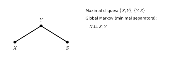
fig_18_1. Download: PDF · SVGDefinition 18.B (separation) p. 282
Let \(A\), \(B\), \(C\) be disjoint subsets of \(V\), with \(A\) and \(B\) non-empty. \(C\) separates \(A\) and \(B\) if every path from a vertex of \(A\) to a vertex of \(B\) contains a vertex of \(C\). Equivalently: after deleting the vertices of \(C\) (and their edges), no vertex of \(A\) is connected to a vertex of \(B\).
In Figure 18.2, \(\{X\}\) separates \(\{Y,W\}\) and \(\{Z\}\), and \(\{X,Y\}\) separates \(W\) and \(Z\) (so does \(\{X\}\) alone).
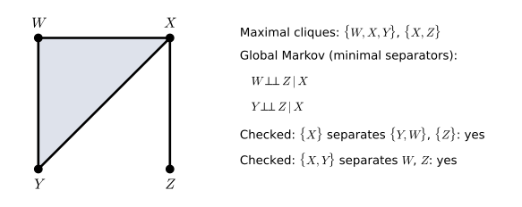
fig_18_2. Download: PDF · SVGFilling the gap 18.1: how to check separation, and four facts used later p. 282
Checking. Delete \(C\), then find every vertex reachable from \(A\) by breadth-first (or depth-first) search; \(C\) separates \(A\) and \(B\) exactly when none of them lies in \(B\). This takes time proportional to \(|V|+|E|\), however many paths there are (the code's separates is confirmed against a brute-force enumeration of all paths on random graphs).
- The empty separator. \(\emptyset\) separates \(A\) and \(B\) exactly when no path joins them, i.e. they lie in different connected components. This is the convention of Remark 18.2.
- Enlarging the separator. If \(C\) separates \(A\) and \(B\) and \(D\) is disjoint from \(A\cup B\), then \(C\cup D\) separates them.
- Shrinking the separated sets. If \(C\) separates \(A\) and \(B\), it separates every non-empty \(A'\subseteq A\) and \(B'\subseteq B\).
- Neighbours separate. For every vertex \(v\), \(\nei(v)\) separates \(v\) from \(V\setminus\cl(v)\) (when that set is non-empty).
The book asks for "distinct" subsets; they must be disjoint, since a variable in \(A\cap B\) is never independent of itself (unless it is constant), and a variable of \(C\) in \(A\) is trivially separated.
Proofs
(1) With \(C=\emptyset\) the condition reads "every path from \(A\) to \(B\) contains a vertex of the empty set", which holds exactly when there is no such path. (2) A path that meets \(C\) meets \(C\cup D\). (3) Paths from \(A'\) to \(B'\) are paths from \(A\) to \(B\). (4) A path from \(v\) to a vertex \(w\notin\cl(v)\) has at least one more vertex after \(v\), and that second vertex is adjacent to \(v\), so it lies in \(\nei(v)\); it is not \(w\), since \(w\) is not a neighbour. ∎
18.2 Probability and Graphs
p. 282 The link between graphs and distributions is conditional independence. We recall its definition and the one tool that makes every proof in this chapter short.
Definition 18.C (conditional independence) and the factorisation criterion
\(X\indep Y\given Z\) if \(f(x,y\given z)=f(x\given z)f(y\given z)\) for all \(x,y\) and every \(z\) with \(f(z)>0\) (Definition 2.9). Criterion: \(X\indep Y\given Z\) if and only if
\[ f(x,y,z)=g(x,z)\,h(y,z)\quad\text{for all }x,y,z \]for some nonnegative functions \(g\) and \(h\). No normalisation of \(g\) or \(h\) is required.
Proof of the criterion
If \(X\indep Y\given Z\), take \(g(x,z)=f(x\given z)f(z)\) and \(h(y,z)=f(y\given z)\) where \(f(z)>0\); where \(f(z)=0\), both sides vanish with \(g=0\). Conversely, suppose \(f=gh\). Summing (or integrating) out \(x\), \(y\) or both gives \(f(y,z)=G(z)h(y,z)\), \(f(x,z)=g(x,z)H(z)\) and \(f(z)=G(z)H(z)\), with \(G(z)=\sum_xg(x,z)\) and \(H(z)=\sum_yh(y,z)\). For \(f(z)>0\),
\[ f(x\given z)f(y\given z)=\frac{g(x,z)H(z)\,G(z)h(y,z)}{G(z)^2H(z)^2}=\frac{g(x,z)h(y,z)}{G(z)H(z)}=\frac{f(x,y,z)}{f(z)}=f(x,y\given z). \]∎
Filling the gap 18.2: the rules of conditional independence, and where positivity enters
For random vectors \(X,Y,Z,W\) with a joint density or mass function:
- Symmetry: \(X\indep Y\given Z\Rightarrow Y\indep X\given Z\).
- Decomposition: \(X\indep(Y,W)\given Z\Rightarrow X\indep Y\given Z\).
- Weak union: \(X\indep(Y,W)\given Z\Rightarrow X\indep Y\given(Z,W)\).
- Contraction: \(X\indep Y\given Z\) and \(X\indep W\given(Y,Z)\Rightarrow X\indep(Y,W)\given Z\).
- Intersection (needs \(f>0\)): \(X\indep Y\given(Z,W)\) and \(X\indep W\given(Z,Y)\Rightarrow X\indep(Y,W)\given Z\).
Rules 1 to 4 hold for every distribution. Rule 5 fails without positivity: if \(X=Y=W\) is one fair coin and \(Z\) is constant, then given \(W\) (or \(Y\)) the variable \(X\) is a constant, so both hypotheses hold, yet \(X\) is not independent of \((Y,W)\). This single failure is the reason for every positivity assumption in the chapter.
Proofs
All use the criterion of Definition 18.C. (1) The criterion is symmetric in \(x\) and \(y\). (2) From \(f(x,y,w,z)=g(x,z)h(y,w,z)\), sum over \(w\): \(f(x,y,z)=g(x,z)\sum_wh(y,w,z)\). (3) The same factorisation \(g(x,z)\cdot h(y,w,z)\) is a product of a function of \((x,(z,w))\) and one of \((y,(z,w))\). (4) Wherever \(f(y,z)>0\), \(f(x,y,w,z)=f(w\given x,y,z)f(x,y,z)\), and the hypotheses give \(f(w\given x,y,z)=f(w\given y,z)\) and \(f(x,y,z)=f(x\given z)f(y,z)\); so \(f(x,y,w,z)\)
(5) With \(f>0\) all conditionals are defined everywhere. The hypotheses say \(f(x\given y,z,w)=f(x\given z,w)\) and \(f(x\given y,z,w)=f(x\given z,y)\) for all arguments, so \(f(x\given z,w)=f(x\given z,y)\) for all \(y,w\). Fix \(y=y_0\): the right side does not depend on \(w\), so \(f(x\given z,w)=a(x,z)\) and therefore \(f(x\given y,z,w)=a(x,z)\) for all \(y,w\). A conditional density of \(X\) given \((Y,W,Z)\) that depends only on \(z\) means \(X\indep(Y,W)\given Z\). Without positivity, \(f(x\given z,w)=f(x\given z,y)\) only holds for pairs \((y,w)\) that occur together, and the coin example shows the conclusion can fail. ∎
The same rules, for directed graphs, are Result 11.7 of Foundations of Deep Learning.
pp. 282–283 Given a distribution \(\P\) of the variables in \(V\), build a graph with one vertex per variable and omit the edge between \(X\) and \(Y\) exactly when they are independent given the rest:
\[ \text{no edge between }X\text{ and }Y\iff X\indep Y\given\rest . \]This is the pairwise Markov graph of \(\P\). Figures 18.3 to 18.6 show examples.
Definition 18.D (pairwise Markov property) pp. 282–284
\(\P\) satisfies the pairwise Markov property with respect to \(\Gc\) if
\[ X\not\sim Y\ \Longrightarrow\ X\indep Y\given\rest\qquad\text{for every pair }X\ne Y. \]The graph built above is the smallest graph (fewest edges) for which \(\P\) has this property (Filling the gap 18.3).
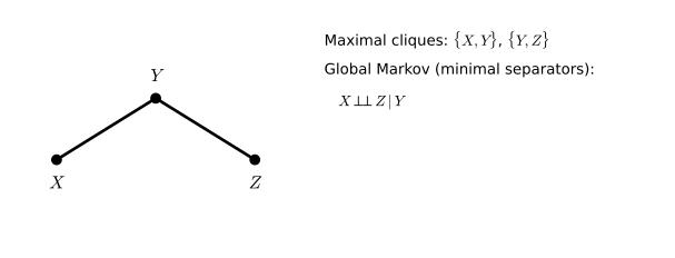
fig_18_3. Download: PDF · SVG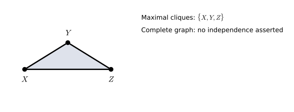
fig_18_4. Download: PDF · SVG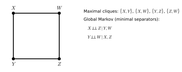
fig_18_5. Download: PDF · SVG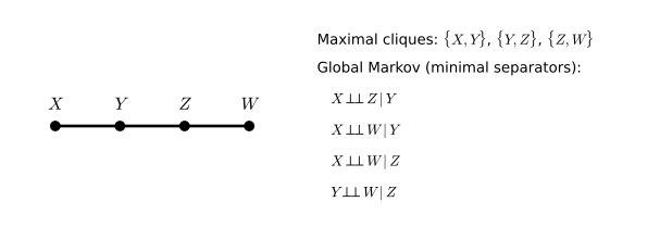
fig_18_6. Download: PDF · SVGFilling the gap 18.3: what the double arrow means pp. 282–283
Read as a recipe, the display "no edge \(\iff X\indep Y\given\rest\)" defines one graph per distribution, \(\Gc(\P)\): the edge \(X\sim Y\) is present exactly when \(X\nindep Y\given\rest\). As a property of a pair \((\P,\Gc)\), only one direction is useful: \(\P\) is pairwise Markov with respect to \(\Gc\) when every missing edge of \(\Gc\) is a conditional independence. The two readings are related by:
\(\P\) is pairwise Markov with respect to \(\Gc\) \(\iff\) \(\Gc\) contains every edge of \(\Gc(\P)\).
So \(\Gc(\P)\) is the unique smallest graph for which \(\P\) is pairwise Markov, and adding edges never breaks the property; the complete graph works for every \(\P\). The one-way reading is the one used by every theorem below (and by the companion courses, see Filling the gap 17.1 there). Filling the gap 18.5 shows what goes wrong with the two-way reading in Theorem 18.3.
Proof
If \(\P\) is pairwise Markov with respect to \(\Gc\) and \(X\sim Y\) in \(\Gc(\P)\), then \(X\nindep Y\given\rest\), so the edge cannot be missing from \(\Gc\). Conversely, if \(\Gc\supseteq\Gc(\P)\) and \(X\not\sim Y\) in \(\Gc\), then \(X\not\sim Y\) in \(\Gc(\P)\), i.e. \(X\indep Y\given\rest\). ∎
p. 283 A graph encodes pairwise statements; these imply others. The next theorem reads them off the graph.
Theorem 18.1 (separation implies conditional independence) p. 283
Let \(\P\) have a positive density or mass function and satisfy the pairwise Markov property with respect to \(\Gc=(V,E)\). If \(A\), \(B\), \(C\) are disjoint subsets of \(V\), \(A\) and \(B\) non-empty, and \(C\) separates \(A\) and \(B\), then \(A\indep B\given C\).
The positivity assumption is missing in the book and cannot be dropped (Filling the gap 18.4).
Proof (backward induction on the size of the separator)
Let \(p=|V|\). We prove the claim for all triples with \(|C|=k\), for \(k=p-2,p-3,\dots,0\) in turn; the rules used are those of Filling the gap 18.2.
Start, \(|C|=p-2\). Then \(A=\{a\}\) and \(B=\{b\}\) are single vertices, \(C\) is the rest, and \(a\not\sim b\) (an edge would be a path avoiding \(C\)). The pairwise property gives \(a\indep b\given C\).
Step. Assume the claim for all separators with more than \(k\) elements, and let \(|C|=k<p-2\).
Case 1: \(A\cup B\cup C=V\). Then \(|A|+|B|=p-k\ge3\), so one of them, say \(A\), has at least two vertices; pick \(\alpha\in A\) and put \(A'=A\setminus\{\alpha\}\). Every path from \(A'\) to \(B\) meets \(C\), hence meets \(C\cup\{\alpha\}\); and every path from \(\alpha\) to \(B\) meets \(C\subseteq C\cup A'\). Both separators are larger than \(C\), so by induction \(B\indep A'\given C\cup\{\alpha\}\) and \(B\indep\alpha\given C\cup A'\). Intersection (positivity) gives \(B\indep(A',\alpha)\given C\), i.e. \(A\indep B\given C\).
Case 2: some \(\gamma\notin A\cup B\cup C\). \(C\cup\{\gamma\}\) still separates \(A\) and \(B\), so by induction \(A\indep B\given C\cup\{\gamma\}\). The vertex \(\gamma\) cannot be joined both to \(A\) and to \(B\) by paths avoiding \(C\) (joining the two paths would give a path from \(A\) to \(B\) avoiding \(C\)). If \(\gamma\) is not so joined to \(A\), every path from \(A\) to \(\gamma\) meets \(C\subseteq B\cup C\), so by induction \(A\indep\gamma\given B\cup C\). Intersection gives \(A\indep(B,\gamma)\given C\), and decomposition gives \(A\indep B\given C\). If \(\gamma\) is not joined to \(B\), exchange the roles of \(A\) and \(B\). ∎
The same induction is written out in Result 17.1 of the companion course. A second proof goes through Hammersley-Clifford: positivity and the pairwise property give the factorisation \((18.1)\) (part (b) of Theorem 18.H uses nothing else), and factorisation gives separation statements (part (a)).
Remark 18.2 (disconnected sets) p. 283
If no path joins \(A\) and \(B\), they are separated by \(\emptyset\) (Filling the gap 18.1(1)), and Theorem 18.1 gives \(A\indep B\): variables in different connected components are independent.
p. 284 The conclusion of Theorem 18.1 is the global Markov property. Between the pairwise and global properties sits a third one, which the book does not name but which is often the most natural.
Definition 18.E (pairwise, local and global Markov properties) p. 284
For a graph \(\Gc\), let \(\Mpair(\Gc)\), \(\Mloc(\Gc)\) and \(\Mglob(\Gc)\) be the sets of distributions \(\P\) with, respectively:
- pairwise: \(X\not\sim Y\Rightarrow X\indep Y\given\rest\);
- local: \(v\indep V\setminus\cl(v)\given\nei(v)\) for every vertex \(v\) (a variable is independent of everything else given its neighbours);
- global: \(C\) separates \(A\) and \(B\) \(\Rightarrow A\indep B\given C\), for disjoint \(A,B,C\).
The book defines \(\Mpair\) and \(\Mglob\) with "if and only if" in place of \(\Rightarrow\); see Filling the gap 18.5 for why that version of Theorem 18.3 is false.
Theorem 18.F (how the three properties relate)
(a) For every distribution, global \(\Rightarrow\) local \(\Rightarrow\) pairwise: \(\Mglob(\Gc)\subseteq\Mloc(\Gc)\subseteq\Mpair(\Gc)\).
(b) For positive distributions the three coincide.
Proof
(a) Global \(\Rightarrow\) local: \(\nei(v)\) separates \(v\) from \(V\setminus\cl(v)\) (Filling the gap 18.1(4)). Local \(\Rightarrow\) pairwise: let \(w\not\sim v\), so \(w\in V\setminus\cl(v)\); write \(V\setminus\cl(v)=\{w\}\cup R\). The local property \(v\indep(w,R)\given\nei(v)\) and weak union give \(v\indep w\given\nei(v)\cup R\), and \(\nei(v)\cup R\) is everything except \(v\) and \(w\).
(b) Theorem 18.1 is "pairwise \(\Rightarrow\) global" for positive distributions; combined with (a) the circle closes. ∎
Result 8.11 of Bayesian and Probabilistic Machine Learning proves the same chain.
Theorem 18.3 (pairwise and global properties agree) p. 284
For every graph \(\Gc\), a positive distribution belongs to \(\Mpair(\Gc)\) if and only if it belongs to \(\Mglob(\Gc)\).
This is Theorem 18.F(b). It lets us build a graph from the simple pairwise statements and then read off everything else. Back in Figure 18.6: \(Y\) separates \(X\) and \(Z\), and \(Z\) separates \(Y\) and \(W\), so \(X\indep Z\given Y\) and \(Y\indep W\given Z\).
Filling the gap 18.4: without positivity, pairwise does not imply global pp. 283–284
Three copies. Let \(X=Y=Z\) be one fair coin, and \(\Gc\) the graph on \(\{X,Y,Z\}\) with no edges. Given any one variable the other two are constants, so all three pairwise statements hold: \(\P\in\Mpair(\Gc)\). But \(\emptyset\) separates \(X\) and \(Y\) while \(I(X;Y)=\log2\ne0\): the global (and the local) property fails.
The chain of Figure 18.6. Let \(Y\) be a fair coin and \(X=Z=W\) a second, independent one. The three pairwise statements of the chain hold (each conditioning set contains \(Z\) or \(W\), which determines the others), yet \(X\nindep Z\given Y\), although \(Y\) separates them.
Near the boundary. Let each copy differ from a common coin with probability \(\eta\). For \(\eta>0\) the distribution is positive, and then (Theorem 18.1) it cannot be pairwise Markov to the empty graph. Figure 18.S1(a) shows the conditional mutual informations: the pairwise one, \(I(X;Y\given Z)\), tends to 0 like \(\eta\log(1/\eta)\), while the global one, \(I(X;Y)\), tends to \(\log2\). With data from \(\eta=0.001\), a test of the pairwise statement needs several hundred observations before it can see the dependence, while the marginal dependence is obvious from a handful: the pairwise graph is a poor summary of such a distribution.
Derivation
Conditional mutual information,
\[ I(A;B\given C)=\sum_{a,b,c}f(a,b,c)\log\frac{f(a,b,c)f(c)}{f(a,c)f(b,c)}, \]is a Kullback-Leibler divergence, nonnegative and zero exactly when \(A\indep B\given C\) (Gibbs' inequality, Result 4.10); the code uses it to decide each statement. For three identical fair coins, \(f(x,y)=\tfrac12\ind\{x=y\}\), so \(I(X;Y)=\sum_x\tfrac12\log\{(1/2)/(1/4)\}\)
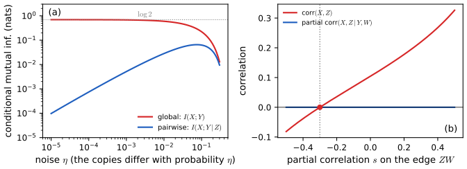
fig_18_s1. Download: PDF · SVGFilling the gap 18.5: with "if and only if" in both definitions, Theorem 18.3 is false p. 284
The book defines \(\P\in\Mpair(\Gc)\) by "\(X\indep Y\given\rest\) if and only if there is no edge", and \(\P\in\Mglob(\Gc)\) by "\(A\indep B\given C\) if and only if \(C\) separates \(A\) and \(B\)". With these definitions one inclusion survives and the other fails, even for positive (Gaussian) distributions.
What survives: \(\Mglob^{\iff}(\Gc)\subseteq\Mpair^{\iff}(\Gc)\), because "rest" separates \(X\) and \(Y\) exactly when they are not adjacent.
What fails. Take the four-cycle \(X-Y-Z-W-X\) of Figure 18.5 and the Gaussian with unit-diagonal precision matrix \(K\) (order \(X,Y,Z,W\)) having \(K_{XY}=K_{YZ}=K_{XW}=-r\), \(K_{ZW}=-s\), and zeros for the two missing edges. Then
\[ \Sigma_{XZ}=\frac{K_{XY}K_{YZ}+K_{XW}K_{WZ}}{\det K}=\frac{r^2+rs}{\det K}, \]a sum over the two paths from \(X\) to \(Z\). At \(s=-r\) (with \(r=0.3\), say) the paths cancel: \(\Sigma_{XZ}=0\), so \(X\indep Z\) (uncorrelated Gaussians are independent), although \(\emptyset\) does not separate them. All four edges have non-zero partial correlations and the two non-edges have zero ones, so \(\P\) is pairwise Markov in the two-way sense; it is not globally Markov in the two-way sense. Figure 18.S1(b).
Why this is rare. Such cancellations need an exact equation among the parameters (here \(s=-r\)); for parameters drawn from any continuous distribution they occur with probability 0. Distributions without them are called faithful to the graph. The correct theorem uses one-way definitions, as in Definition 18.E, and then needs positivity, as in Theorem 18.3.
Derivation of \(\Sigma_{XZ}\)
For a symmetric matrix, \((K^{-1})_{XZ}=C_{XZ}/\det K\), where the cofactor \(C_{XZ}=(-1)^{1+3}\det M\), with \(M\) the matrix \(K\) without row \(Z\) and column \(X\). Deleting row 3 and column 1 of
\[ K=\begin{pmatrix}1&a&0&b\\a&1&c&0\\0&c&1&d\\b&0&d&1\end{pmatrix}\ \text{ leaves }\ \begin{pmatrix}a&0&b\\1&c&0\\0&d&1\end{pmatrix}, \]whose determinant is \(a(c-0)-0+b(d-0)=ac+bd\). With \(a=b=c=-r\), \(d=-s\) this is \(r^2+rs\). Positive definiteness at \(r=0.3\), \(s=-0.3\): the smallest eigenvalue of \(K\) is 0.58. ∎
p. 284 Two more examples of reading a graph.
Example 18.4. p. 284 In Figure 18.7, \(X\) is isolated, so \(\emptyset\) separates \(X\) from \(Y\), from \(Z\), and from \(\{Y,Z\}\): \(X\indep Y\), \(X\indep Z\) and \(X\indep(Y,Z)\) (Remark 18.2).
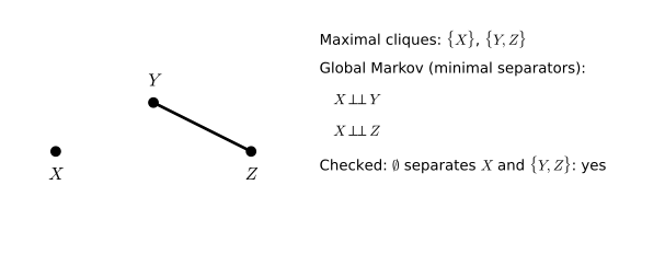
fig_18_7. Download: PDF · SVGExample 18.5. p. 284 In Figure 18.8, every path from \(X\) passes through \(Y\), so \(X\indep W\given(Y,Z)\), \(X\indep Z\given Y\), and indeed \(X\indep(Z,W)\given Y\).
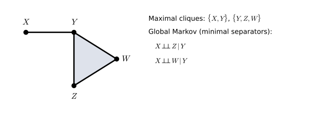
fig_18_8. Download: PDF · SVGFilling the gap 18.6: listing everything a graph says pp. 283–285
A graph asserts infinitely many statements in principle (all disjoint triples with separation), but for pairs of vertices a finite list says it all: for each non-adjacent pair \(a,b\), the minimal separators, sets \(C\) that separate \(a\) and \(b\) and from which no vertex can be removed. By Filling the gap 18.1(2), every superset of a minimal separator (avoiding \(a,b\)) also separates, and every separator contains a minimal one, so
\(C\) separates \(a\) and \(b\) \(\iff\) \(C\) contains a minimal separator of \(a\) and \(b\).
The figures list these for each graph (the code finds them by searching subsets in order of size). Statements between sets of vertices follow from separation directly, as in Example 18.4. In the demonstration, each graph's pairwise, local and global statements are tested on a distribution you choose.
Proof of the equivalence
If \(C\) contains a minimal separator \(C_0\), then \(C=C_0\cup(C\setminus C_0)\) separates by Filling the gap 18.1(2). If \(C\) separates, remove vertices from \(C\) one at a time as long as the remaining set still separates; the process stops at a minimal separator contained in \(C\). ∎
18.3 Cliques and Potentials
p. 285 The Markov properties restrict a distribution by independence statements. The equivalent description by a formula uses cliques.
Definition 18.G (clique, maximal clique, potential) p. 285
A clique is a set of vertices that are all adjacent to each other (a complete subset). A clique is maximal if no other vertex can be added to it with the result still a clique. A potential is any positive function. \(\P\) factorises according to \(\Gc\) if its density or mass function can be written
\[ f(x)=\frac{\prod_{C\in\Cc}\psi_C(x_C)}{Z} \tag{18.1} \]where \(\Cc\) is the set of maximal cliques, each \(\psi_C\) is a potential (a positive function of the variables in \(C\) only), and \(Z=\sum_x\prod_{C\in\Cc}\psi_C(x_C)\) (an integral for continuous variables) is the normalising constant.
Theorem 18.H (Hammersley-Clifford; Hammersley and Clifford, 1971; Besag, 1974) p. 285
(a) If \(f\) factorises as \((18.1)\) (with nonnegative \(\psi_C\), not necessarily positive), then \(\P\) satisfies the global Markov property with respect to \(\Gc\).
(b) If \(f\) is positive and satisfies the pairwise Markov property with respect to \(\Gc\), then \(f\) factorises as \((18.1)\) with positive potentials.
Hence a positive \(\P\) is Markov to \(\Gc\) (pairwise, local or global, which are then equivalent) if and only if \((18.1)\) holds. These are the "certain conditions" of the book.
Proof of (a), the easy direction
Let \(C\) separate \(A\) and \(B\) (disjoint, \(A,B\) non-empty). Let \(\tilde A\) be the set of vertices outside \(C\) that can be reached from \(A\) by a path avoiding \(C\) (so \(A\subseteq\tilde A\)), and \(\tilde B=V\setminus(\tilde A\cup C)\); then \(B\subseteq\tilde B\), by separation. No edge joins \(\tilde A\) to \(\tilde B\): if \(u\in\tilde A\) were adjacent to \(w\in\tilde B\), then \(w\) could be reached from \(A\) avoiding \(C\), so \(w\in\tilde A\). Therefore no clique meets both \(\tilde A\) and \(\tilde B\), and every maximal clique lies inside \(\tilde A\cup C\) or inside \(\tilde B\cup C\). Grouping the factors of \((18.1)\) accordingly,
\[ f(x)=\underbrace{\frac1Z\prod_{C'\subseteq\tilde A\cup C}\psi_{C'}(x_{C'})}_{g(x_{\tilde A},\,x_C)}\ \underbrace{\prod_{C'\not\subseteq\tilde A\cup C}\psi_{C'}(x_{C'})}_{h(x_{\tilde B},\,x_C)} , \]so \(\tilde A\indep\tilde B\given C\) by the factorisation criterion (Definition 18.C), and \(A\indep B\given C\) by decomposition. Nothing here used positivity. ∎
Proof of (b), by Möbius inversion
Fix a reference configuration \(x^*\). For \(U\subseteq V\) write \(g_U(x)=\log f(x_U,x^*_{V\setminus U})\), the log-density at the point that agrees with \(x\) on \(U\) and with \(x^*\) elsewhere (finite because \(f>0\)). For every \(S\subseteq V\) define
\[ H_S(x)=\sum_{U\subseteq S}(-1)^{|S\setminus U|}g_U(x). \]Step 1: \(H_S\) depends on \(x\) only through \(x_S\), because each \(g_U\) with \(U\subseteq S\) does.
Step 2: \(\log f=\sum_SH_S\). Swapping sums,
\[ \sum_{S\subseteq V}H_S=\sum_{U\subseteq V}g_U\sum_{S:\,U\subseteq S\subseteq V}(-1)^{|S\setminus U|}. \]The inner sum is \(\sum_{k=0}^{m}\binom mk(-1)^k=(1-1)^m\) with \(m=|V\setminus U|\): it is 0 unless \(U=V\), when it is 1. So the total is \(g_V(x)=\log f(x)\).
Step 3: \(H_S\equiv0\) unless \(S\) is a clique. Suppose \(i,j\in S\) are not adjacent and put \(T=S\setminus\{i,j\}\). Grouping the subsets of \(S\) by their trace on \(T\),
\[ H_S(x)=\sum_{U\subseteq T}(-1)^{|T\setminus U|}\big[g_{U\cup\{i,j\}}-g_{U\cup\{i\}}-g_{U\cup\{j\}}+g_U\big](x). \]Each bracket is 0. Let \(w\) denote the values of all variables other than \(i,j\) (equal to \(x\) on \(U\) and to \(x^*\) off it). The bracket is \(\log\frac{f(x_i,x_j,w)\,f(x_i^*,x_j^*,w)}{f(x_i,x_j^*,w)\,f(x_i^*,x_j,w)}\). By the pairwise property \(X_i\indep X_j\given\rest\), the ratio \(f(x_i,x_j,w)/f(x_i^*,x_j,w)\)
Step 4: grouping. By Steps 2 and 3, \(\log f(x)=\sum_{S\text{ clique}}H_S(x_S)\) (with \(H_\emptyset=\log f(x^*)\), a constant). Assign every non-empty clique to one maximal clique containing it, and let \(\log\psi_C\) be the sum of the \(H_S\) assigned to \(C\). This is \((18.1)\) with \(Z=1/f(x^*)\) and positive potentials. ∎
The same argument, with the cancellation in four terms written out at greater length, is Result 8.13 of the companion course; Result 17.2 of another gives a shorter outline.
Filling the gap 18.7: what potentials are, and are not p. 285
- Not unique. Multiplying one potential by a constant and dividing \(Z\) by it changes nothing; and if two maximal cliques share a vertex \(v\), any positive function \(a(x_v)\) can be moved from one potential to the other. The interaction terms \(H_S\) of the proof are unique once \(x^*\) is fixed (Filling the gap 18.9).
- Not marginals. In general \(\psi_C(x_C)\) is not proportional to the marginal \(f(x_C)\). For the path \(X-Y-Z\) of Example 18.6 one valid choice is \(\psi_1=f(x,y)\) and \(\psi_2=f(z\given y)\), since \(f(x,y,z)=f(x,y)f(z\given y)\); but \(\psi_2=f(y,z)\) would count the marginal of \(Y\) twice. For graphs whose cliques can be arranged in a tree (decomposable graphs), \(f=\prod_Cf(x_C)/\prod_Sf(x_S)\) with \(S\) running over the separators between neighbouring cliques; the graph of Figure 18.9 is not of this kind, because the cycle \(X_1-X_2-X_5-X_3-X_1\) has no chord.
- Non-maximal cliques are allowed. A product of positive functions over any cliques (not only maximal ones) is of the form \((18.1)\), by grouping. Pairwise models such as the Ising model of the demos, \(f(x)\propto\exp(J\sum_{i\sim j}s_is_j+h\sum_is_i)\) with \(s=2x-1\), are therefore Markov to their graph even when the graph has triangles.
- The normalising constant \(Z\) is a sum over all \(2^{|V|}\) configurations for binary variables: easy for the graphs here, the main computational difficulty for large graphs.
The book's display \((18.1)\) should be followed by the words "\(\psi_C\) is a potential", as the author's errata note.
Filling the gap 18.8: Hammersley-Clifford without positivity p. 285
Part (a) needs no positivity: potentials that vanish on some configurations still give the global property. Part (b) does: Moussouris (1974) gave a distribution on the four-cycle \(X_1-X_2-X_3-X_4-X_1\) with eight equally likely binary configurations (0000, 1000, 1100, 1110, 1111, 0111, 0011, 0001) which satisfies the global Markov property but does not factorise. The configuration 0010 has probability 0, yet each of its four edge patterns occurs in a configuration of positive probability, so any factorisation \(\psi_{12}\psi_{23}\psi_{34}\psi_{41}\) would give it a positive value. The full argument is Filling the gap 8.8 of the companion course; the code confirms both facts.
Example 18.6. p. 285 The maximal cliques of Figure 18.1 are \(C_1=\{X,Y\}\) and \(C_2=\{Y,Z\}\). So if \(\P\) is Markov to the graph and positive,
\[ f(x,y,z)\propto\psi_1(x,y)\,\psi_2(y,z) \]for some positive functions \(\psi_1,\psi_2\). Conversely, any such product is Markov to the graph, i.e. \(X\indep Z\given Y\).
Example 18.7. p. 286 The maximal cliques of Figure 18.9 are \(\{X_1,X_2\}\), \(\{X_1,X_3\}\), \(\{X_2,X_4\}\), \(\{X_3,X_5\}\) and \(\{X_2,X_5,X_6\}\), so
\[ f(x_1,\dots,x_6)\propto\psi_{12}(x_1,x_2)\,\psi_{13}(x_1,x_3)\,\psi_{24}(x_2,x_4)\,\psi_{35}(x_3,x_5)\,\psi_{256}(x_2,x_5,x_6). \]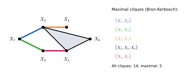
fig_18_9. Download: PDF · SVGFilling the gap 18.9: interaction terms, finding cliques, and counting parameters pp. 285–286
Interaction terms for binary variables. Take \(x_v\in\{0,1\}\) and the reference \(x^*=0\). Then \(H_S(x)\) is zero unless \(x_S=1_S\), and the proof of Theorem 18.H says that every positive \(f\) can be written uniquely as
\[ \log f(x)=\log f(0)+\sum_{\emptyset\ne S\subseteq V}\lambda_S\prod_{v\in S}x_v,\qquad \lambda_S=\sum_{U\subseteq S}(-1)^{|S\setminus U|}\log f(1_U,0_{V\setminus U}), \]and that \(f\) is Markov to \(\Gc\) if and only if \(\lambda_S=0\) for every \(S\) that is not a clique. This is the log-linear model of the book's Chapter 19 in its "corner" parametrisation, and it turns Hammersley-Clifford into something you can compute: Figure 18.S4 shows the 63 terms for a distribution built from random potentials on Figure 18.9.
Counting parameters. So the positive binary distributions Markov to \(\Gc\) form a family with one free parameter per non-empty clique: 14 for Figure 18.9 instead of \(2^6-1=63\) for an arbitrary distribution, 8 for the four-cycle, 7 (no restriction) for the triangle.
Finding the maximal cliques. The Bron-Kerbosch algorithm grows a clique \(R\) from a set \(P\) of candidates (vertices adjacent to all of \(R\)) and a set \(X\) of excluded vertices; it reports \(R\) when \(P\) and \(X\) are both empty, and otherwise branches on the candidates not adjacent to a pivot vertex. Each maximal clique is reported once. In the worst case a graph on \(p\) vertices has \(3^{p/3}\) maximal cliques, and the pivoting version runs in time of that order (Tomita, Tanaka and Takahashi, 2006). The code's version is checked against brute force on random graphs.
Derivations
The binary formula. With \(x^*=0\), \(g_U(x)=\log f(x_U,0)\). If \(x_v=0\) for some \(v\in S\), then \(g_U=g_{U\cup\{v\}}\) for every \(U\subseteq S\setminus\{v\}\), and these pairs cancel in \(H_S\) (their signs differ), so \(H_S(x)=0\). If \(x_S=1_S\), \(H_S(x)=\lambda_S\) as displayed. Summing, \(\log f(x)=\sum_SH_S(x)\)
Uniqueness. The \(2^{|V|}\) functions \(x\mapsto\prod_{v\in S}x_v\) (\(S\subseteq V\)) are linearly independent on \(\{0,1\}^V\) (evaluate at \(x=1_U\) for \(U\) in increasing order of size: the system is triangular with unit diagonal), so the coefficients are determined by \(\log f\).
Markov iff zero outside cliques. If \(f\) is Markov and positive, Step 3 of the proof of Theorem 18.H gives \(\lambda_S=H_S(1)=0\) for non-cliques. Conversely, if \(\lambda_S=0\) off the cliques, \(f\) is a product of positive functions of cliques, hence Markov by Theorem 18.H(a).
The count. The \(\lambda_S\) for the non-empty cliques are free real numbers, and \(\log f(0)\) is then fixed by normalisation; distinct parameter vectors give distinct distributions by uniqueness. ∎
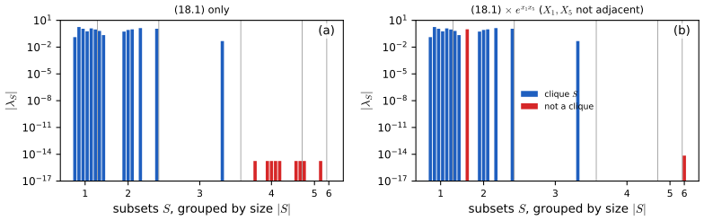
fig_18_s4. Download: PDF · SVG18.4 Fitting Graphs to Data
p. 286 Given data, which graph? The book leaves this "big topic" aside and points to log-linear models (its Chapter 19) for discrete data. The simplest approach, and the one used in the exercises, is to test each missing edge: decide for each pair whether \(X\indep Y\given\rest\) is compatible with the data, keep the edges where it is rejected, and then read further independences off the resulting graph by Theorem 18.1. The two subsections below give the tests for contingency tables and for Gaussian data. Penalised likelihood (the graphical lasso) is the main alternative for many variables; it is covered in Section 17.3.2 of a companion course.
18.4.1 Testing conditional independence in a contingency table (added)
Let \(X\), \(Y\), \(Z\) be discrete with \(I\), \(J\), \(K\) values, and \(n_{ijk}\) the counts in a sample of size \(n\) (multinomial with cell probabilities \(p_{ijk}\)). Write \(n_{i+k}=\sum_jn_{ijk}\), \(n_{+jk}=\sum_in_{ijk}\), \(n_{++k}=\sum_{i,j}n_{ijk}\). In a graph, \(Z\) stands for "the rest" of the variables (all their joint values form the strata).
Theorem 18.I (likelihood ratio test of conditional independence; Exercise 18.4)
Under \(H_0:X\indep Y\given Z\) the MLE of the cell probabilities is \(\hat p_{ijk}=n_{i+k}n_{+jk}/(n\,n_{++k})\), and the likelihood ratio statistic is
\[ G^2=2\sum_{i,j,k}n_{ijk}\log\frac{n_{ijk}\,n_{++k}}{n_{i+k}\,n_{+jk}}=2n\,\hat I(X;Y\given Z), \]where \(\hat I\) is the conditional mutual information of the empirical distribution. If every \(p_{ijk}>0\), under \(H_0\) \(G^2\) converges in distribution to \(\chi^2_\nu\) with \(\nu=K(I-1)(J-1)\). The test rejects when \(G^2>\chi^2_{\nu,\alpha}\). Pearson's statistic \(\sum(n_{ijk}-n\hat p_{ijk})^2/(n\hat p_{ijk})\) has the same limit.
Proof
MLE under \(H_0\). Write \(p_{ijk}=p_{k}\,p_{i\given k}\,p_{j\given k}\). The log-likelihood
\[ \sum n_{ijk}\log p_{ijk}=\sum_kn_{++k}\log p_k+\sum_{i,k}n_{i+k}\log p_{i\given k}+\sum_{j,k}n_{+jk}\log p_{j\given k} \]splits into separate multinomial log-likelihoods, maximised by \(\hat p_k=n_{++k}/n\), \(\hat p_{i\given k}=n_{i+k}/n_{++k}\), \(\hat p_{j\given k}=n_{+jk}/n_{++k}\). The product is the stated \(\hat p_{ijk}\).
The statistic. The unrestricted MLE is \(n_{ijk}/n\), so \(G^2=2\sum n_{ijk}\log\{(n_{ijk}/n)/\hat p_{ijk}\}\), which simplifies to the display. With \(\hat f(i,j,k)=n_{ijk}/n\), the sum is \(n\) times
\[ \sum_{i,j,k}\hat f(i,j,k)\log\frac{\hat f(i,j,k)\hat f(k)}{\hat f(i,k)\hat f(j,k)}=\hat I(X;Y\given Z). \]Degrees of freedom. The full model has \(IJK-1\) free parameters; \(H_0\) has \((K-1)+K(I-1)+K(J-1)\). The difference is \(IJK-K(I+J-1)\)
In sparse tables, strata with \(n_{++k}=0\) contribute nothing and should be removed from \(\nu\); and the \(\chi^2\) approximation needs most expected counts \(n\hat p_{ijk}\) to be at least about 5. The breast cancer data of Exercise 18.5 are well within that range.
18.4.2 Gaussian graphical models (added)
For continuous data the standard model is the multivariate Normal, \(X\sim\N_p(\mu,\Sigma)\) with \(\Sigma\) positive definite, and the graph is encoded by the precision matrix \(K=\Sigma^{-1}\). A Gaussian density is positive, so all Markov properties coincide (Theorem 18.F).
Theorem 18.J (zeros of the precision matrix are missing edges)
For \(X\sim\N_p(\mu,\Sigma)\) and \(j\ne k\): \(X_j\indep X_k\given\rest\) if and only if \(K_{jk}=0\). So the pairwise Markov graph of a Gaussian has an edge exactly where \(K\) has a non-zero off-diagonal entry, and every separation in that graph is a conditional independence.
Proof
The density is proportional to \(\exp\{-\tfrac12\sum_{a,b}K_{ab}(x_a-\mu_a)\)
The same result with the regression interpretation is Result 17.4 of the companion course, and its precision-zeros demo shows the zero pattern of \(K\) against the (usually full) pattern of \(\Sigma\).
Theorem 18.K (partial correlations)
Let \(a=\{j,k\}\) and \(b\) the other \(p-2\) indices.
(a) \(\Cov(X_a\given X_b)=\Sigma_{aa}-\Sigma_{ab}\Sigma_{bb}^{-1}\Sigma_{ba}\)
(b) In the regression of \(X_j\) on all the other variables, the coefficient of \(X_k\) is \(\beta_{jk}=-K_{jk}/K_{jj}\), and the residual variance is \(1/K_{jj}\); hence \(\rho_{jk\cdot\rest}^2=\beta_{jk}\beta_{kj}\).
(c) For data, the sample partial correlation \(r_{jk\cdot\rest}=-\hat K_{jk}/\sqrt{\hat K_{jj}\hat K_{kk}}\), with \(\hat K\) the inverse of the sample covariance matrix, equals the sample correlation between the residuals of \(X_j\) and of \(X_k\) after least-squares regression (with intercept) on the other \(p-2\) variables.
Proof
(a) The conditional covariance formula is part of Result 2.16. From \(K\Sigma=I\), the \((a,b)\) and \((a,a)\) blocks give \(K_{aa}\Sigma_{ab}+K_{ab}\Sigma_{bb}=0\) and \(K_{aa}\Sigma_{aa}+K_{ab}\Sigma_{ba}=I\). The first gives \(K_{ab}=-K_{aa}\Sigma_{ab}\Sigma_{bb}^{-1}\); substituting in the second, \(K_{aa}(\Sigma_{aa}-\Sigma_{ab}\Sigma_{bb}^{-1}\Sigma_{ba})=I\). For a \(2\times2\) matrix \(M=\big(\begin{smallmatrix}u&w\\w&v\end{smallmatrix}\big)\), \(M^{-1}=\big(\begin{smallmatrix}v&-w\\-w&u\end{smallmatrix}\big)/(uv-w^2)\), whose correlation is \(-w/\sqrt{uv}\); with \(M=K_{aa}\) this is the formula.
(b) Apply (a) with \(a=\{j\}\): \(\V(X_j\given\rest)=1/K_{jj}\), and the conditional mean is \(\mu_j+\Sigma_{jb}\Sigma_{bb}^{-1}(x_b-\mu_b)\) with \(\Sigma_{jb}\Sigma_{bb}^{-1}=-K_{jj}^{-1}K_{jb}\) (from the identity \(K_{ab}=-K_{aa}\Sigma_{ab}\Sigma_{bb}^{-1}\) above). Then \(\beta_{jk}\beta_{kj}=K_{jk}^2/(K_{jj}K_{kk})\).
(c) Let \(D\) be the \(n\times(p-1)\) matrix of ones and the other \(p-2\) columns, and \(e_j\), \(e_k\) the residual vectors of the two columns after projection on \(D\). Then \([e_j\ e_k]^\T[e_j\ e_k]\) is the Schur complement \(Q_{aa}-Q_{ab}Q_{bb}^{-1}Q_{ba}\) of the centred cross-product matrix \(Q=(n-1)S\) (projecting on the intercept centres the columns, and projecting the centred columns on the rest gives the Schur complement). By the identity of (a) applied to \(Q\), it equals \(((Q^{-1})_{aa})^{-1}\), and the correlation of its two columns is \(-(Q^{-1})_{jk}/\sqrt{(Q^{-1})_{jj}(Q^{-1})_{kk}}\)
Theorem 18.L (the exact test of a partial correlation)
Let \(X_1,\dots,X_n\) be independent \(\N_p(\mu,\Sigma)\) vectors with \(n>p\), and \(r=r_{jk\cdot\rest}\) the sample partial correlation. If \(K_{jk}=0\), then
\[ t=r\sqrt{\frac{n-p}{1-r^2}}\ \sim\ t_{n-p}\quad\text{exactly.} \]The test that rejects "no edge between \(j\) and \(k\)" when \(|t|>t_{n-p,\alpha/2}\) has size exactly \(\alpha\). It is the usual \(t\) test of the coefficient of \(X_k\) in the least-squares regression of \(X_j\) on the other \(p-1\) variables.
Proof
Conditioning. Fix the columns other than \(j\); call the matrix of ones and those \(p-1\) columns \(D\) (it has full rank \(p\) with probability one when \(n>p\)). Given \(D\), by Theorem 18.K(b) the column \(X_j\) follows a linear model \(X_j=D\gamma+\varepsilon\), \(\varepsilon\sim\N(0,\sigma^2I_n)\), \(\sigma^2=1/K_{jj}\), in which the coefficient of \(X_k\) is \(\beta_{jk}=-K_{jk}/K_{jj}=0\) under the hypothesis. In a Gaussian linear model with fixed full-rank design, the \(t\) statistic of a zero coefficient has the \(t_{n-p}\) distribution, \(n-p\) being the residual degrees of freedom (the estimate is Normal and independent of the residual sum of squares, which is \(\sigma^2\chi^2_{n-p}\); see the book's Chapter 13 and Result 3.4 of a companion course). This conditional distribution does not depend on \(D\), so it is also the unconditional distribution.
The regression \(t\) is a function of \(r\) (Frisch-Waugh-Lovell). Let \(e_j\), \(e_k\) be the residuals of \(X_j\) and \(X_k\) on the other \(p-2\) columns and the intercept. The coefficient of \(X_k\) in the full regression is \(\hat\beta=e_k^\T e_j/e_k^\T e_k\); the residual sum of squares is \(e_j^\T e_j-(e_k^\T e_j)^2/e_k^\T e_k=e_j^\T e_j(1-r^2)\), with \(r\) the correlation of \(e_j\) and \(e_k\) (Theorem 18.K(c)); and the standard error is \(\hat\sigma/\|e_k\|\) with \(\hat\sigma^2=e_j^\T e_j(1-r^2)/(n-p)\). Therefore
\[ t=\frac{\hat\beta\,\|e_k\|}{\hat\sigma}=\frac{e_k^\T e_j/\|e_k\|}{\|e_j\|\sqrt{(1-r^2)/(n-p)}}=r\sqrt{\frac{n-p}{1-r^2}} . \]∎ The code confirms the identity against the regression \(t\) statistics of a standard least-squares routine, and the \(t_{n-p}\) law by simulation (Figure 18.S3(a)).
Filling the gap 18.10: Fisher's \(z\), and what "large \(n\)" means here
A common alternative is Fisher's transformation: \(z=\sqrt{n-q-3}\,\atanh(r)\) is approximately \(\N(0,1)\) when the true partial correlation is 0, with \(q=p-2\) conditioning variables. Because \(|z|>c\) exactly when \(|r|>\tanh(c/\sqrt{n-p-1})\), and \(r\) maps one-to-one onto \(t\), its exact size is
\[ \P(|z|>z_{\alpha/2})=\P\Big(|T_{n-p}|>\frac{\rho_c\sqrt{n-p}}{\sqrt{1-\rho_c^2}}\Big),\qquad \rho_c=\tanh\frac{z_{\alpha/2}}{\sqrt{n-p-1}} . \]For \(p=6\) and \(\alpha=0.05\) the size is 0.039 at \(n=8\) and between 0.0499 and 0.0511 for every \(n\) from 10 to 200: Fisher's \(z\) is remarkably accurate. The real danger is using the \(t\) statistic with a Normal cut-off 1.96, whose size is 0.19 at \(n=8\), 0.098 at \(n=12\) and 0.070 at \(n=20\) (Figure 18.S3(b)). With many variables the degrees of freedom \(n-p\), not \(n\), are what matter.
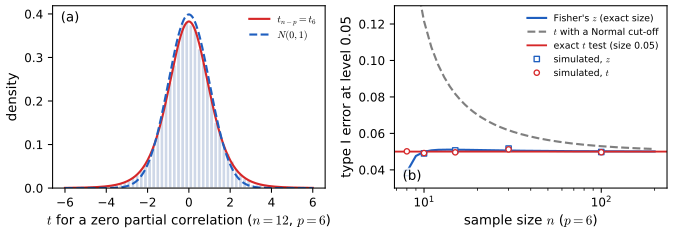
fig_18_s3. Download: PDF · SVGFilling the gap 18.11: from tests to a graph
Edge exclusion. Test each of the \(m=p(p-1)/2\) pairs and keep the edge when "no edge" is rejected. Each test asks about one pairwise statement, given all other variables, so for Gaussian data the result estimates the pairwise Markov graph, and Theorem 18.1 then supplies every separation statement.
Multiplicity. With \(m\) tests at level \(\alpha\), about \(\alpha\) times the number of truly missing edges will be included by mistake. Bonferroni (reject when \(p_{jk}<\alpha/m\), Theorem 10.24) bounds the probability of including any spurious edge by \(\alpha\); Benjamini-Hochberg (Theorem 10.26) controls the expected proportion of spurious edges among those included (under independence or positive dependence of the tests; the Benjamini-Yekutieli variant works in general).
Caveats. A non-rejected test is not evidence of independence, only of too little information to see dependence; the graph found depends on \(n\). Testing marginal correlations instead gives a different graph, the covariance graph (an edge where \(\Sigma_{jk}\ne0\)), which is usually much denser: in a chain every pair is correlated.
Example: the coris data. For the eight continuous variables of the book's South African heart disease data (462 men; tobacco and alcohol on the scale \(\log(1+x)\)), 11 of the 28 partial correlations are significant at 5% and 7 survive Bonferroni (Figure 18.S2). Two contrasts with the marginal correlations stand out: obesity and age are positively correlated (\(+0.29\)) but have a negative partial correlation (\(-0.25\)), because both are strongly linked to adiposity (\(+0.69\) and \(+0.51\)); and blood pressure and LDL cholesterol are correlated (\(+0.16\)) but have partial correlation 0.000, consistent with \(\text{sbp}\indep\text{ldl}\given\rest\). With Bonferroni, the marginal correlations would give 17 edges.
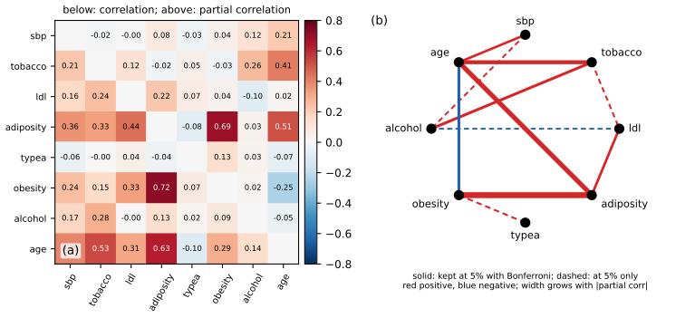
fig_18_s2. Download: PDF · SVG18.5 Bibliographic Remarks
p. 286 Whittaker (1990) and Lauritzen (1996) give thorough treatments of undirected graphs; some of the exercises come from Whittaker. The separation theorem goes back to Pearl and Paz (1987) in the form of the rules of Filling the gap 18.2; the factorisation theorem to Hammersley and Clifford (1971, unpublished) and Besag (1974), with the non-positive counterexample of Moussouris (1974). Gaussian graphical models (covariance selection) start with Dempster (1972); the test of a partial correlation is classical (Fisher, 1924; Anderson, 2003, Chapter 4).
Notes on the book
Two slips of Chapter 18 are in the author's errata list; the other points are mine, each with the evidence.
Page 285, after (18.1): the phrase "\(\psi_C\) is a potential" is missing
Listed in the author's errata (item 44 of the first list). See Definition 18.G.
Page 286, caption of Figure 18.9: "maximumly cliques" should be "maximal cliques"
Listed in the author's errata (item 45 of the first list).
Page 284: the definition of \(\Mglob(\Gc)\) is written with \(\Mpair\)
The sentence that defines the set of globally Markov distributions reads "thus \(\P\in\Mpair(\Gc)\) if, under \(\P\), \(A\indep B\given C\) if and only if \(C\) separates \(A\) and \(B\)"; it should read \(\P\in\Mglob(\Gc)\), otherwise Theorem 18.3 compares a set with itself. Not in the errata lists.
Pages 283–285: Theorems 18.1 and 18.3 need a positive distribution
Theorem 18.1 is false without positivity: three identical fair coins satisfy all pairwise statements of the graph with no edges, but no two of them are independent (Filling the gap 18.4, Figure 18.S1(a), and the demonstration). The book's later phrase "under certain conditions" in Section 18.3 refers to the same assumption. Not in the errata lists.
Page 284: with "if and only if" definitions, Theorem 18.3 is false even for positive distributions
A Gaussian on the four-cycle with partial correlations \(0.3,0.3,0.3,-0.3\) on its edges has \(X\indep Z\) because the two paths from \(X\) to \(Z\) cancel; it satisfies the book's two-way pairwise definition but not its two-way global one (Filling the gap 18.5, Figure 18.S1(b)). The theorem is correct with one-way definitions and positivity, as in Theorem 18.3 here. Not in the errata lists.
Page 282: "distinct subsets" should be "disjoint subsets"
If \(A\) and \(B\) share a non-constant variable, \(A\indep B\given C\) is false whatever \(C\) is, while the separation condition can hold (for instance with \(C\) containing the shared vertex). Theorem 18.1 needs \(A\), \(B\), \(C\) disjoint and \(A\), \(B\) non-empty. Not in the errata lists.
18.6 Exercises
All five exercises of Chapter 18 (Wasserman, 2004, pp. 286–289), restated in my own words, with complete solutions (hidden). In Exercises 1 and 2, "draw a graph that has the given relations" is read as: the pairwise Markov graph when the listed statements are all the pairwise ones that hold, so the missing edges are exactly the listed pairs.
Exercise 18.1. For three variables \(X_1,X_2,X_3\), draw a graph with: (a) \(X_1\indep X_3\given X_2\); (b) \(X_1\indep X_2\given X_3\) and \(X_1\indep X_3\given X_2\); (c) all three statements \(X_1\indep X_2\given X_3\), \(X_1\indep X_3\given X_2\), \(X_2\indep X_3\given X_1\).
Solution
With three variables, "given the rest" means given the third, so each statement removes one edge from the triangle. (a) The path \(X_1-X_2-X_3\). (b) Only the edge \(X_2-X_3\) is left; \(X_1\) is isolated. For a positive distribution Remark 18.2 then gives the stronger \(X_1\indep(X_2,X_3)\), which is the intersection rule of Filling the gap 18.2 applied to the two given statements. (c) No edges: for positive distributions the three variables are mutually independent. (For the non-positive \(X_1=X_2=X_3\), all three statements of (c) hold but the variables are not independent: Filling the gap 18.4.)
Exercise 18.2. For four variables, draw a graph with: (a) \(X_1\indep X_3\given X_2,X_4\), \(X_1\indep X_4\given X_2,X_3\), \(X_2\indep X_4\given X_1,X_3\); (b) \(X_1\indep X_2\given X_3,X_4\), \(X_1\indep X_3\given X_2,X_4\), \(X_2\indep X_3\given X_1,X_4\); (c) \(X_1\indep X_3\given X_2,X_4\) and \(X_2\indep X_4\given X_1,X_3\).
Solution
Start from the complete graph on four vertices (six edges) and remove the listed pairs. (a) Removing 13, 14, 24 leaves 12, 23, 34: the chain \(X_1-X_2-X_3-X_4\) of Figure 18.11. (b) Removing 12, 13, 23 leaves 14, 24, 34: a star with centre \(X_4\), so \(X_1,X_2,X_3\) are mutually independent given \(X_4\) (for positive distributions). (c) Removing 13 and 24 leaves the four-cycle \(X_1-X_2-X_3-X_4-X_1\), as in Figures 18.5 and 18.12.
Exercise 18.3. A conditional independence between two variables is minimal if no variable can be dropped from its conditioning set and still give a separation (Whittaker, 1990). List the minimal conditional independences of the graphs in Figures 18.10 to 18.13.
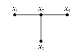
Figure 18.10. A star with centre \(X_2\). Reproduces Wasserman (2004), Figure 18.10. Code: fig_18_10. Download: PDF · SVG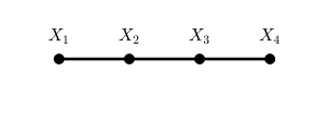
Figure 18.11. The chain \(X_1-X_2-X_3-X_4\). Reproduces Wasserman (2004), Figure 18.11. Code: fig_18_11. Download: PDF · SVG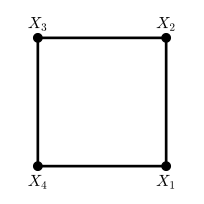
Figure 18.12. A four-cycle. Reproduces Wasserman (2004), Figure 18.12. Code: fig_18_12. Download: PDF · SVG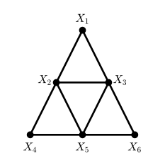
Figure 18.13. Four triangles. Reproduces Wasserman (2004), Figure 18.13. Code: fig_18_13. Download: PDF · SVGSolution
By Filling the gap 18.6, the minimal independences are \(a\indep b\given C\) for each non-adjacent pair \(a,b\) and each minimal separator \(C\). Found by inspection and confirmed by the code (
minimal_separators):(a) Figure 18.10: \(X_1\indep X_3\given X_2\), \(X_1\indep X_4\given X_2\), \(X_3\indep X_4\given X_2\).
(b) Figure 18.11: \(X_1\indep X_3\given X_2\); \(X_1\indep X_4\given X_2\) and \(X_1\indep X_4\given X_3\) (two different minimal separators); \(X_2\indep X_4\given X_3\).
(c) Figure 18.12: \(X_1\indep X_3\given\{X_2,X_4\}\) and \(X_2\indep X_4\given\{X_1,X_3\}\); no single vertex separates opposite corners of a cycle.
(d) Figure 18.13 (maximal cliques \(\{X_1,X_2,X_3\}\), \(\{X_2,X_3,X_5\}\), \(\{X_2,X_4,X_5\}\), \(\{X_3,X_5,X_6\}\)): \(X_1\indep X_4\given\{X_2,X_3\}\) and \(X_1\indep X_4\given\{X_2,X_5\}\); \(X_1\indep X_5\given\{X_2,X_3\}\); \(X_1\indep X_6\given\{X_2,X_3\}\) and \(X_1\indep X_6\given\{X_3,X_5\}\); \(X_2\indep X_6\given\{X_3,X_5\}\); \(X_3\indep X_4\given\{X_2,X_5\}\); \(X_4\indep X_6\given\{X_2,X_5\}\) and \(X_4\indep X_6\given\{X_3,X_5\}\). Nine statements; no single vertex separates any pair, since the graph stays connected after deleting any one vertex.
Exercise 18.4. For binary \(X_1,X_2,X_3\), construct the likelihood ratio test of \(H_0:X_1\indep X_2\given X_3\) against the alternative that this independence fails.
Solution
This is Theorem 18.I with \(I=J=K=2\). From a sample of \(n\) with counts \(n_{ijk}\), compute
\[ G^2=2\sum_{i,j,k\in\{0,1\}}n_{ijk}\log\frac{n_{ijk}\,n_{++k}}{n_{i+k}\,n_{+jk}}, \]the sum of the two \(2\times2\) independence statistics, one for each value of \(X_3\). Under \(H_0\) (with all cell probabilities positive) \(G^2\to\chi^2_2\) in distribution, since \(\nu=2\cdot1\cdot1=2\): reject at level \(\alpha\) when \(G^2>\chi^2_{2,\alpha}\) (5.99 for \(\alpha=0.05\)), and the \(p\)-value is \(\P(\chi^2_2>G^2)=e^{-G^2/2}\). A simulation with \(n=500\) and a distribution satisfying \(H_0\) gives rejection rate 0.0525 at the 5% level over 4000 tables, and the simulated statistics pass a Kolmogorov-Smirnov test against \(\chi^2_2\).
Exercise 18.5. Breast cancer data (Morrison et al., 1973): diagnostic centre \(X_1\), nuclear grade \(X_2\), survival \(X_3\).
malignant, died malignant, survived benign, died benign, survived Boston 35 59 47 112 Glamorgan 42 77 26 76 (a) Treating the table as one multinomial sample, find the MLE. (b) Estimate the probability of death for a patient at Glamorgan whose tumour is graded benign, with a standard error. (c) Test each of \(X_1\indep X_2\given X_3\), \(X_1\indep X_3\given X_2\), \(X_2\indep X_3\given X_1\) with the test of Exercise 18.4; draw and interpret the resulting graph.
Solution
(a) \(n=474\) and \(\hat p_{ijk}=n_{ijk}/474\):
malignant, died malignant, survived benign, died benign, survived Boston 0.0738 0.1245 0.0992 0.2363 Glamorgan 0.0886 0.1624 0.0549 0.1603 (b) By equivariance of the MLE, the estimated probability of death for a benign tumour at Glamorgan is
\[ \hat\theta=\frac{\hat p_{\mathrm{G,b,d}}}{\hat p_{\mathrm{G,b,d}}+\hat p_{\mathrm{G,b,s}}}=\frac{26}{102}=0.255 . \]The multivariate delta method (Theorem 5.15) with the multinomial covariance \((\mathrm{diag}(p)-pp^\T)/n\) and the gradient of \(\theta=p_1/(p_1+p_2)\), \(\big(p_2,-p_1\big)/(p_1+p_2)^2\), gives \(\widehat{\mathrm{se}}^2=\hat\theta(1-\hat\theta)/102\): the same as treating the 102 Glamorgan benign cases as a binomial sample. So \(\widehat{\mathrm{se}}=0.0432\), and an approximate 95% interval is \(0.255\pm0.085\), i.e. \((0.17,0.34)\).
(c) Each statistic has \(2\) degrees of freedom:
hypothesis \(G^2\) Pearson \(X^2\) \(p\)-value edge centre \(\indep\) grade \(\given\) survival 13.78 13.72 0.0010 kept centre \(\indep\) survival \(\given\) grade 0.60 0.60 0.741 removed grade \(\indep\) survival \(\given\) centre 4.07 4.07 0.131 removed The resulting graph has the single edge \(X_1-X_2\), with \(X_3\) isolated (Figure 18.S5). Read by Remark 18.2, it says survival is independent of centre and grade jointly; a direct test of \(X_3\indep(X_1,X_2)\) agrees (\(G^2=4.22\) on 3 degrees of freedom, \(p=0.24\)). Centre and grade are associated: the proportion of tumours graded benign is \(159/253=0.63\) in Boston and \(102/221=0.46\) in Glamorgan, which could reflect different patients or different grading practice. Two cautions: the grade-survival test is not far from significance, so "no edge" means "no evidence of an edge at this sample size"; and the three tests were run separately at 5% without a correction.
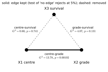
fig_18_s5. Download: PDF · SVGDemonstrations for this chapter
Each demonstration runs in the browser and links back to these notes. The ▶ Demo boxes above open them already set to the case under discussion.
| Demonstration | What you can see | Sections and results |
|---|---|---|
| Pairwise versus global Markov properties | A binary distribution on a small graph (a positive Ising model, noisy copies of one coin, or the breast cancer data); its probability table; and every pairwise, local and global statement of the graph with its conditional mutual information and likelihood ratio test. Presets: 1 a positive chain; 2 three identical coins; 3 nearly identical coins; 4 the chain counterexample; 5 Exercise 18.5. | 18.2; Theorem 18.1, 18.F, 18.I; Filling the gap 18.4 |
| Cliques, potentials and interaction terms | Random positive potentials on the maximal cliques of a graph, the resulting distribution, all its interaction terms \(\lambda_S\), and the effect of an extra interaction on a non-clique. Presets: 1 Example 18.6; 2 the four-cycle; 3 Example 18.7; 4 a chord that is not there; 5 Figure 18.S4(b). | 18.3; Theorem 18.H; Filling the gaps 18.7, 18.9 |
| A graph from partial correlations | Correlations and partial correlations of the coris data or of simulated Gaussian data; exact \(t\) tests with or without multiplicity correction; the fitted graph, compared with the true one for simulated data. Presets: 1 coris at 5%; 2 Bonferroni; 3 marginal correlations; 4 a simulated chain; 5 the chain by marginal correlations. | 18.4.2; Theorems 18.J–18.L; Filling the gap 18.11 |
Related demonstrations in the companion courses: zeros of the precision matrix (separating sets and Algorithm 17.1 for a known graph) and the graphical lasso of Statistical Learning: Theory and Methods, and the image denoising demo (an Ising Markov random field) and the d-separation demo (the directed counterpart of separation) of Bayesian and Probabilistic Machine Learning. The Python code that produces every figure of this page is code/ch18_undirected_graphs.py (see the code index).
References
- Wasserman, L. (2004). All of Statistics: A Concise Course in Statistical Inference. Springer, New York. Chapter 18, pp. 281–289. www.stat.cmu.edu/~larry/all-of-statistics.
- Anderson, T. W. (2003). An Introduction to Multivariate Statistical Analysis, 3rd edition. Wiley, Hoboken.
- Benjamini, Y. and Yekutieli, D. (2001). The control of the false discovery rate in multiple testing under dependency. The Annals of Statistics, 29(4), 1165–1188.
- Besag, J. (1974). Spatial interaction and the statistical analysis of lattice systems. Journal of the Royal Statistical Society, Series B, 36(2), 192–236.
- Bron, C. and Kerbosch, J. (1973). Algorithm 457: finding all cliques of an undirected graph. Communications of the ACM, 16(9), 575–577.
- Dempster, A. P. (1972). Covariance selection. Biometrics, 28(1), 157–175.
- Fisher, R. A. (1924). The distribution of the partial correlation coefficient. Metron, 3, 329–332.
- Hammersley, J. M. and Clifford, P. (1971). Markov fields on finite graphs and lattices. Unpublished manuscript.
- Lauritzen, S. L. (1996). Graphical Models. Oxford University Press, Oxford.
- Morrison, A. S., Black, M. M., Lowe, C. R., MacMahon, B. and Yuasa, S. (1973). Some international differences in histology and survival in breast cancer. International Journal of Cancer, 11(2), 261–267.
- Moussouris, J. (1974). Gibbs and Markov random systems with constraints. Journal of Statistical Physics, 10(1), 11–33.
- Pearl, J. and Paz, A. (1987). Graphoids: a graph-based logic for reasoning about relevance relations. In Advances in Artificial Intelligence II, 357–363. North-Holland, Amsterdam.
- Tomita, E., Tanaka, A. and Takahashi, H. (2006). The worst-case time complexity for generating all maximal cliques and computational experiments. Theoretical Computer Science, 363(1), 28–42.
- Whittaker, J. (1990). Graphical Models in Applied Multivariate Statistics. Wiley, Chichester.
The numerical statements in the text (the separations, minimal separators and maximal cliques of every figure, the counterexamples of Filling the gaps 18.4, 18.5 and 18.8, the interaction terms and parameter counts, the likelihood ratio statistics and their null distribution, the partial-correlation identities, the exact sizes of the tests, the coris graph and the solutions of the exercises) were confirmed numerically.