Directed Graphs and Conditional Independence
A directed acyclic graph is a compact way to write down a joint distribution: each variable is drawn given its parents, and the arrows that are missing are statements of conditional independence. This chapter of the book introduces conditional independence, the factorisation a graph defines, the Markov condition, d-separation for reading further independences off the graph, Markov equivalence, and, in its appendix, interventions, which turn a graph into a causal model. The book states the main theorems without proof. These notes prove them: the rules of conditional independence (including when the last one fails), the equivalence of factorisation and the Markov condition, the correctness of the reachability algorithm for d-separation, the characterisation of Markov equivalence through covered edges, the decomposition of the likelihood, and, in full, the calculus of interventions: the truncated factorisation, the adjustment formula, randomisation, unidentifiability under hidden confounding, and the exact link with the counterfactuals of Chapter 16.
Ch. 1 Probability Ch. 2 Random variables Ch. 3 Expectation Ch. 4 Inequalities Ch. 5 Convergence Ch. 6 Models and inference Ch. 7 Estimating the CDF Ch. 8 Bootstrap Ch. 9 Parametric inference Ch. 10 Hypothesis testing Ch. 11 Bayesian inference Ch. 12 Decision theory Ch. 13 Regression Ch. 14 Multivariate models Ch. 15 Independence Ch. 16 Causal inference Ch. 17 Directed graphs Ch. 18 Undirected graphs Ch. 19 Log-linear models Ch. 20 Curve estimation Ch. 21 Orthogonal functions Ch. 22 Classification Ch. 23 Stochastic processes Ch. 24 Simulation
How to read these notes
They follow the book. Sections carry the book's numbers (17.1 to 17.9) and every displayed equation that appears in the book carries the book's own equation number, e.g. \((17.3)\). Numbered items keep the book's numbers (Definition 17.3, Theorem 17.6, Example 17.9); results the book states without a number, and the new results needed to fill its gaps, are lettered (Lemma 17.A, Definition 17.B, Theorem 17.D, ...). Equations without a number are steps that the book skips.
Filling the gaps. Wherever the book says "it can be shown", quotes a result without proof, or leaves an argument implicit, an orange Filling the gap box gives the full argument. Proofs and derivations start hidden: open one with its bar, or use the button below.
Figures and demonstrations. All twelve figures of the chapter are graphs; they are redrawn by the Python code, which also computes the independence statements and probabilities printed on them. Six supplementary figures (17.S1 to 17.S6) illustrate gaps filled in the notes. The ▶ Demo boxes open an interactive demonstration already set to the case being discussed.
Main reference
L. Wasserman, All of Statistics: A Concise Course in Statistical Inference, Springer (2004), Chapter 17, pages 263–279 (book website: www.stat.cmu.edu/~larry/all-of-statistics). Section, equation, example and exercise numbers below refer to this book. Further reading is listed in the references.
The explanations, derivations, figures and code are my own; equations are cited by their numbers in the book.
Companion courses
Directed graphs are treated at length in two companion courses on this site, from the machine-learning side. The overlapping material is:
- Bayesian and Probabilistic Machine Learning, Chapter 8: DAGs and their factorisation (Section 8.1, Results 8.1 and 8.2), conditional independence and the factorisation criterion (Result 8.6), the three basic graphs (Results 8.7 and 8.8), d-separation with a full proof of its soundness (Result 8.9), the number of DAGs (Result 8.24) and structure learning (Section 8.4.8). Its d-separation demo lists every path and where it is blocked.
- Foundations of Deep Learning, Chapter 11: the factorisation (Result 11.1), linear-Gaussian graphs (Result 11.4), conditional independence (Result 11.7), explaining away (Section 11.2.2), d-separation (Result 11.10, with the reachability search as Algorithm 11.1) and the equality of the two "filters" (Result 11.14). Its demos: explaining away and linear-Gaussian DAGs.
- Statistical Learning: Theory and Methods, Chapter 17: undirected graphical models (Markov graphs and the Hammersley-Clifford theorem, Result 17.2), the undirected counterpart of this chapter, covered by Chapter 18 of the book.
Where a proof there is complete, these notes give the statement, a short argument and the link. New here: the rules of conditional independence with the role of positivity (Theorem 17.2, Filling the gap 17.3), a direct proof that factorisation and the Markov condition agree (17.5), deriving hidden independences from the rules alone (17.6), faithfulness and its failure (17.8), Markov equivalence proved through covered edges (17.9), the tie of equivalent DAGs in estimation (Theorem 17.D), and the whole of the appendix: interventions (Definition 17.C, Theorem 17.E), the adjustment formula (Theorem 17.F), randomised and observational studies (17.13) and counterfactuals (17.14).
The chapter at a glance
- 17.2 \(X\indep Y\given Z\) means the conditional joint factorises (Definition 17.1); it obeys five rules (Theorem 17.2), the last only for positive distributions.
- 17.3–17.4 A DAG represents the distributions \(f(v)=\prod_if(x_i\given\pa_i)\) (Definition 17.3), exactly those in which every variable is independent of its non-descendants given its parents (Theorem 17.6).
- 17.5 All the independences a DAG implies are read off by d-separation (Definition 17.B, Theorem 17.10), computable in linear time (Algorithm 17.A). Different DAGs can imply the same independences; they do exactly when they share skeleton and unshielded colliders (Theorem 17.13).
- 17.6 The likelihood of a DAG splits into one term per variable; equivalent DAGs fit every data set equally well (Theorem 17.D), so data alone identify at most an equivalence class.
- 17.8 Intervening ("set \(X=x\)") deletes the factor of \(X\) (Definition 17.C); this differs from conditioning on \(X=x\) unless there is no confounding, and the causal effect is the average of \(f(y\given x,\pa_X)\) over the parents of \(X\) (Theorem 17.F).
Notation. \(V=(X_1,\dots,X_k)\) are the variables of a graph \(\cG\) (vertices and variables are identified). \(f\) is a probability mass function or density; \(f(x\given z)=f(x,z)/f(z)\) wherever \(f(z)>0\). \(\pa_i=\pa(X_i)\) are the parents of \(X_i\), and also their values. \(\an(S)\) is the set \(S\) together with its ancestors, \(\de(S)\) the set \(S\) together with its descendants, and \(\nd(X)=V\setminus\de(\{X\})\) the non-descendants of \(X\). \(\cM(\cG)\) is the set of distributions Markov to \(\cG\), \(\cI(\cG)\) the independence statements it implies. \(P(Y=y\given X\set x)\) is the distribution of \(Y\) after the intervention "set \(X=x\)" (written \(P(y\given\mathrm{do}(x))\) by Pearl). \(\expit(t)=e^t/(1+e^t)\).
Prerequisites. Joint, marginal and conditional distributions and independence (Chapter 2), the multivariate Normal (Result 2.16), iterated expectations (Result 3.11), the bootstrap (Chapter 8) and maximum likelihood (Chapter 9); counterfactuals (Chapter 16) for the appendix. See the course home.
17.1 Introduction
p. 263 A directed graph is a set of nodes joined by arrows. Graphs serve two purposes in this chapter: they encode conditional independence relations among random variables, and, with the extra idea of an intervention (Section 17.8), they encode causal relations, as an alternative to the counterfactuals of Chapter 16. A directed graph equipped with a probability distribution is often called a Bayesian network; the name is misleading, since the inference for such a model may be frequentist or Bayesian.
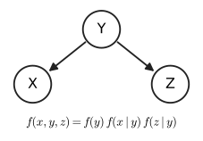
fig_17_1. Download: PDF · SVG17.2 Conditional Independence
Definition 17.1 (conditional independence) p. 264
Random variables \(X\) and \(Y\) are conditionally independent given \(Z\), written \(X\indep Y\given Z\), if
\[ f_{X,Y\given Z}(x,y\given z)=f_{X\given Z}(x\given z)\,f_{Y\given Z}(y\given z) \tag{17.1} \]for all \(x,y\) and all \(z\) with \(f(z)>0\). Equivalently,
\[ f(x\given y,z)=f(x\given z) \tag{17.2} \]for all \(x\) and all \((y,z)\) with \(f(y,z)>0\): once \(Z\) is known, \(Y\) carries no further information about \(X\). Here \(X,Y,Z\) may be vectors; with \(Z\) constant this is ordinary independence (Definition 2.8). For densities, "for all" means "for almost all".
See also (companion courses): Result 8.6 of Bayesian and Probabilistic Machine Learning and Result 11.7 of Foundations of Deep Learning.
Filling the gap 17.1: why (17.1) and (17.2) are equivalent, and the factorisation criterion p. 264; Exercise 17.1
The book asserts the equivalence (Exercise 17.1). It rests on the definition \(f(x\given z)=f(x,z)/f(z)\), and the only care needed is with zero probabilities. A third form is the most useful in practice.
Lemma 17.A (factorisation criterion)
\(X\indep Y\given Z\) if and only if there are functions \(g,h\ge0\) with \(f(x,y,z)=g(x,z)\,h(y,z)\) for all \(x,y,z\).
Proofs
(17.1) implies (17.2). Let \(f(y,z)>0\). Then \(f(z)\ge f(y,z)>0\) (discrete case; for densities integrate) and \(f(y\given z)=f(y,z)/f(z)>0\), so
\[ f(x\given y,z)=\frac{f(x,y,z)}{f(y,z)}=\frac{f(x,y\given z)}{f(y\given z)}=\frac{f(x\given z)f(y\given z)}{f(y\given z)}=f(x\given z). \](17.2) implies (17.1). Fix \(z\) with \(f(z)>0\). If \(f(y\given z)>0\) then \(f(y,z)>0\) and \(f(x,y\given z)\)
Lemma 17.A. If (17.1) holds, take \(g(x,z)=f(x\given z)\) and \(h(y,z)=f(y,z)\) (and \(g=h=0\) where \(f(z)=0\), where \(f(x,y,z)=0\) as well). Conversely put \(G(z)=\sum_xg(x,z)\) and \(H(z)=\sum_yh(y,z)\); summing the factorisation gives \(f(x,z)=g(x,z)H(z)\), \(f(y,z)=G(z)h(y,z)\) and \(f(z)=G(z)H(z)\), hence for \(f(z)>0\)
\[ f(x\given z)f(y\given z)=\frac{g(x,z)H(z)\,G(z)h(y,z)}{G(z)^2H(z)^2}=\frac{f(x,y,z)}{f(z)}=f(x,y\given z). \]The same proof is Result 8.6(a) of the companion course. Numerically, the table of Exercise 17.3 satisfies (17.2) exactly. ∎
Theorem 17.2 (rules of conditional independence) p. 264
Let \(h\) be a function and \(U=h(X)\). Then
- Symmetry: \(X\indep Y\given Z\implies Y\indep X\given Z\).
- Functions (decomposition): \(X\indep Y\given Z\implies U\indep Y\given Z\).
- Weak union: \(X\indep Y\given Z\implies X\indep Y\given(Z,U)\).
- Contraction: \(X\indep Y\given Z\) and \(X\indep W\given(Y,Z)\implies X\indep(W,Y)\given Z\).
- Intersection: if \(f(x,y,z)>0\) for all \(x,y,z\), then \(X\indep Y\given Z\) and \(X\indep Z\given Y\implies X\indep(Y,Z)\).
Rules 1 to 4 hold for every distribution; rule 5 needs positivity (the book's footnote). Taking \(X=(X_1,X_2)\) and \(h\) a coordinate map, rule 2 says that \((X_1,X_2)\indep Y\given Z\) implies \(X_1\indep Y\given Z\), and rule 3 that it implies \(X_1\indep Y\given(Z,X_2)\): these are the usual forms of decomposition and weak union.
Filling the gap 17.2: proof of Theorem 17.2 p. 264; Exercise 17.2
The book gives no proof. Each rule is a short manipulation of Lemma 17.A; the proofs are written for mass functions, and for densities sums become integrals.
Proof
1. (17.1) is symmetric in \(x\) and \(y\).
2. For \(f(z)>0\), \(f(u,y\given z)\)
3. The joint mass function of \((X,Y,Z,U)\) is \(f(x,y,z)\ind\{u=h(x)\}\). Using (17.1), \(f(x,y,z)=f(x,z)f(y\given z)\), so
\[ f(x,y,z,u)=\underbrace{f(x,z)\ind\{u=h(x)\}}_{g(x,(z,u))}\;\underbrace{f(y\given z)}_{k(y,(z,u))}, \]a product of a function of \((x,(z,u))\) and a function of \((y,(z,u))\); Lemma 17.A with conditioning variable \((Z,U)\) gives \(X\indep Y\given(Z,U)\).
4. Where \(f(x,y,z)>0\), the second hypothesis in the form (17.2) gives \(f(w\given x,y,z)=f(w\given y,z)\), and the first gives \(f(x,y,z)=f(x\given z)f(y,z)\). Hence
\[ f(x,w,y,z)=f(w\given x,y,z)\,f(x,y,z)=f(x\given z)\,\big[f(w\given y,z)f(y,z)\big]=g(x,z)\,k\big((w,y),z\big), \]and where \(f(x,y,z)=0\) both sides vanish (take \(k=0\) where \(f(y,z)=0\), and note \(f(x\given z)f(y,z)=f(x,y,z)=0\) otherwise). Lemma 17.A gives \(X\indep(W,Y)\given Z\).
5. With all probabilities positive every conditional is defined. The hypotheses give \(f(x,y,z)=f(x\given z)f(y,z)\) and \(f(x,y,z)=f(x\given y)f(y,z)\); dividing by \(f(y,z)>0\), \(f(x\given z)=f(x\given y)\) for all \(x,y,z\). Fixing \(y=y_0\) shows that \(f(x\given z)=a(x):=f(x\given y_0)\) does not depend on \(z\), so \(f(x,y,z)=a(x)f(y,z)\), a product of a function of \(x\) and a function of \((y,z)\): \(X\indep(Y,Z)\) by Lemma 17.A with a constant conditioning variable. ∎
Filling the gap 17.3: what goes wrong without positivity, and what conditional independence does not say p. 264, footnote 1
(a) Intersection fails without positivity. Let \(X\) be a fair coin and \(Y=Z=X\). Given \(Z\), both \(X\) and \(Y\) are constants, so \(X\indep Y\given Z\); likewise \(X\indep Z\given Y\). But \(X\) is not independent of \((Y,Z)\): it is a function of them, and the mutual information \(I(X;(Y,Z))=\log2\). The proof of rule 5 broke down because \(f(x\given y)\) and \(f(x\given z)\) were compared at \((y,z)=(0,1)\), a pair of probability zero.
(b) Neither conditional nor marginal independence implies the other. In Exercise 17.3, \(X\indep Y\given Z\) but \(X\) and \(Y\) are dependent; in a collider \(X\to Y\leftarrow Z\) (Figure 17.6), \(X\indep Z\) but \(X\) and \(Z\) are dependent given \(Y\). So conditional independence is not a weaker or stronger form of independence; it is a different statement, and the graph tells us which ones hold.
(c) The rules are not complete. Rules 1 to 4 (the semi-graphoid axioms; with rule 5, graphoid, Pearl, 1988) are sound for every distribution, but no finite list of such rules derives every implication between conditional independence statements that holds for all distributions (Studený, 1992). For the statements that come from a DAG, however, they are enough, as Filling the gap 17.6 illustrates.
17.3 DAGs
Definition 17.A (directed graphs and their vocabulary) pp. 264–266
A directed graph \(\cG=(V,E)\) has a vertex set \(V\) and an edge set \(E\) of ordered pairs; \((X,Y)\in E\) is drawn as an arrow \(X\to Y\). Then:
- \(X\) and \(Y\) are adjacent if an arrow joins them (in either direction); \(X\) is a parent of \(Y\), and \(Y\) a child of \(X\), if \(X\to Y\); \(\pa_X\) or \(\pa(X)\) is the set of parents.
- A directed path from \(X\) to \(Y\) is a sequence of arrows all pointing the same way, \(X\to\cdots\to Y\); an undirected path is a sequence of distinct vertices, each adjacent to the next, ignoring directions.
- \(X\) is an ancestor of \(Y\), and \(Y\) a descendant of \(X\), if there is a directed path from \(X\) to \(Y\) or \(X=Y\).
- On a path, a vertex \(Y\) with both neighbours pointing into it, \(X\to Y\leftarrow Z\), is a collider; any other interior vertex (\(X\to Y\to Z\), \(X\leftarrow Y\to Z\), \(X\leftarrow Y\leftarrow Z\)) is a non-collider. Being a collider depends on the path (in Figure 17.7, \(Y\) is a collider on \(X,Y,Z\) but not on \(X,Y,W\)). A collider is unshielded if \(X\) and \(Z\) are not adjacent.
- A directed path from a vertex back to itself is a cycle; a graph without cycles is a directed acyclic graph (DAG). From now on all graphs are DAGs.
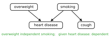
fig_17_2. Download: PDF · SVGLemma 17.B (acyclic means orderable)
A directed graph is acyclic if and only if its vertices can be listed as \(X_1,\dots,X_k\) so that every arrow points from a lower to a higher index (a topological order). In such an order the parents, and more generally the ancestors, of \(X_i\) come before \(X_i\), and its descendants after it.
Proof
If such an order exists, indices strictly increase along every directed path, so no path returns to its start. Conversely, a DAG has a vertex without parents: otherwise, walking backwards from parent to parent would, after more than \(k\) steps, repeat a vertex and close a cycle. Put such a vertex first, delete it (the rest is still acyclic) and repeat. The code's topological_order does exactly this. Same argument: Result 8.1 of the companion course. ∎
17.4 Probability and DAGs
Definition 17.3 (Markov to a DAG) p. 266
Let \(\cG\) be a DAG with vertices \(V=(X_1,\dots,X_k)\). A distribution \(P\) for \(V\) with probability function \(f\) is Markov to \(\cG\) (or \(\cG\) represents \(P\)) if
\[ f(v)=\prod_{i=1}^{k}f(x_i\given\pa_i), \tag{17.3} \]where \(\pa_i\) are the parents of \(X_i\). The set of all such distributions is \(\cM(\cG)\).
Example 17.4. p. 266 For Figure 17.2, abbreviating overweight, smoking, heart disease and cough by their initials, the probability function factorises as \(f(o,s,h,c)\)
Example 17.5. p. 266 For the DAG of Figure 17.3, \(P\in\cM(\cG)\) if and only if \(f(x,y,z,w)=f(x)f(y)f(z\given x,y)f(w\given z)\).
Filling the gap 17.4: (17.3) builds a distribution from any conditional tables, and its factors are its conditionals p. 266
Definition 17.3 uses the conditionals of \(P\) itself. Read the other way, it is a recipe: choose for each \(i\) any conditional probability function \(k_i(x_i\given\pa_i)\) (nonnegative and summing to one over \(x_i\) for every value of the parents) and multiply. Two facts make the recipe sound.
Lemma 17.C (marginals over ancestral sets)
Call \(A\subseteq V\) ancestral if it contains the parents of each of its members. If \(F(v)=\prod_{i=1}^kk_i(x_i\given\pa_i)\), then summing \(F\) over the variables outside an ancestral set \(A\) gives \(\prod_{i\in A}k_i(x_i\given\pa_i)\). In particular (\(A=\varnothing\)) \(F\) is a probability function, and (\(A=\{X_1,\dots,X_j\}\) in a topological order) its conditionals are \(F(x_j\given\pa_j)=k_j(x_j\given\pa_j)\).
Proof
Fix a topological order (Lemma 17.B) and let \(X_m\) be the last vertex outside \(A\). A child of \(X_m\) outside \(A\) would come after it, which is impossible; a child inside \(A\) would make \(X_m\) a parent of a member of \(A\), hence a member of \(A\). So \(X_m\) has no children: \(x_m\) occurs only in the factor \(k_m\), and \(\sum_{x_m}k_m(x_m\given\pa_m)=1\) removes it. Repeat until only \(A\) is left.
For the conditionals: initial segments \(\{X_1,\dots,X_j\}\) of a topological order are ancestral, so \(F(x_1,\dots,x_j)=\prod_{i\le j}k_i\) and dividing two consecutive ones gives \(F(x_j\given x_1,\dots,x_{j-1})=k_j(x_j\given\pa_j)\) (where the denominator is positive). This depends on the predecessors only through \(\pa_j\), so averaging over the other predecessors given \(\pa_j\) leaves it unchanged: \(F(x_j\given\pa_j)=k_j(x_j\given\pa_j)\). For densities the sums are integrals. ∎
So \(\cM(\cG)\) is exactly the set of distributions produced by the recipe, and sampling from it is the "ancestral sampling" of the program on p. 273: draw the variables in a topological order, each given its already drawn parents. Same results in the companion courses: Result 8.2 and Result 11.1.
The next theorem says that factorising and satisfying the Markov condition are the same thing: every variable is independent of its "past" (its non-descendants) once its parents are known.
Theorem 17.6 (factorisation is equivalent to the Markov condition) p. 267
\(P\in\cM(\cG)\) if and only if, for every variable \(W\),
\[ W\indep\widetilde W\given\pa_W, \tag{17.4} \]where \(\widetilde W=\nd(W)\setminus\pa_W\) is the set of all other variables except the parents and the descendants of \(W\).
Filling the gap 17.5: proof of Theorem 17.6 p. 267
The book states the theorem without proof. Both directions follow from Lemma 17.C and the chain rule.
Proof
Factorisation implies (17.4). Let \(A=\{W\}\cup\nd(W)\). It is ancestral: a parent of \(W\) is a non-descendant of \(W\) (acyclicity), and a parent of a non-descendant \(U\) is a non-descendant (if it were a descendant of \(W\), so would be \(U\)). By Lemma 17.C,
\[ f(w,\nd(W))=f(w\given\pa_W)\prod_{U\in\nd(W)}f(u\given\pa_U). \]No factor of the product involves \(w\): \(W\) is not a parent of any non-descendant, because its children are descendants. The right-hand side is therefore \(g(w,\pa_W)\,h(\nd(W))\), and since \(\pa_W\subseteq\nd(W)\), Lemma 17.A with conditioning variable \(\pa_W\) (and the remaining non-descendants \(\widetilde W\) in the role of \(Y\)) gives \(W\indep\widetilde W\given\pa_W\).
(17.4) implies factorisation. List the variables in a topological order. By the chain rule, \(f(v)=\prod_if(x_i\given x_1,\dots,x_{i-1})\). The predecessors of \(X_i\) are non-descendants of \(X_i\) (descendants come later) and include \(\pa_i\). By (17.4) and rule 2 of Theorem 17.2 applied to the coordinates \(\{X_1,\dots,X_{i-1}\}\setminus\pa_i\) of \(\widetilde{X_i}\), \(X_i\indep\{X_1,\dots,X_{i-1}\}\setminus\pa_i\given\pa_i\), that is \(f(x_i\given x_1,\dots,x_{i-1})=f(x_i\given\pa_i)\) by (17.2). Substituting gives (17.3). (Where some \(f(x_1,\dots,x_{i-1})=0\) both sides of (17.3) vanish: by induction on \(i\), \(f(x_1,\dots,x_i)=\prod_{j\le i}f(x_j\given\pa_j)\), so a zero marginal forces a zero factor.) ∎
For random tables on the DAGs of Figures 17.2 to 17.12, every statement (17.4) holds to rounding error (conditional mutual information below \(10^{-15}\)). A different route, through d-separation, is Result 8.9(b) of the companion course.
Example 17.7. p. 267 In Figure 17.3 the Markov condition gives \(X\indep Y\) (the non-descendants of \(X\) are \(Y\), and \(X\) has no parents) and \(W\indep\{X,Y\}\given Z\).
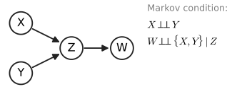
local_markov (a statement that merely mirrors an earlier one, such as \(Y\indep X\), is omitted). Redrawn. Reproduces Wasserman (2004), Figure 17.3. Code: ch17_directed_graphs.py, fig_17_3. Download: PDF · SVGExample 17.8. p. 267 For the DAG of Figure 17.4, \(f(a,b,c,d,e)\)
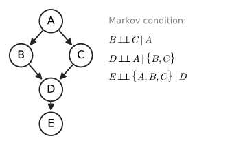
fig_17_4. Download: PDF · SVGThe factorisation also counts parameters: with binary variables, (17.3) for Figure 17.4 needs \(1+2+2+4+2=11\) numbers instead of \(2^5-1=31\) for an unrestricted table (in general \(\sum_i(r_i-1)\prod_{j\in\pa_i}r_j\) for variables with \(r_i\) values; Result 8.4 of the companion course).
17.5 More Independence Relations
pp. 267–268 The Markov condition lists some independences; others follow from them. For the DAG of Figure 17.5 it gives
\[ X_1\indep X_2,\quad X_2\indep\{X_1,X_4\},\quad X_3\indep X_4\given\{X_1,X_2\},\quad X_4\indep\{X_2,X_3\}\given X_1,\quad X_5\indep\{X_1,X_2\}\given\{X_3,X_4\}, \]and these imply \(\{X_4,X_5\}\indep X_2\given\{X_1,X_3\}\), which is not on the list.
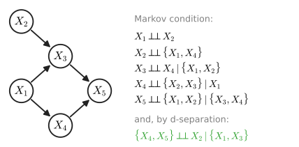
fig_17_5. Download: PDF · SVGFilling the gap 17.6: the hidden independence of Figure 17.5, from the rules alone p. 268
The book says the extra relation follows from the five statements "but it is not obvious". Two of them and two rules of Theorem 17.2 suffice.
- \(X_4\indep\{X_2,X_3\}\given X_1\) gives, by weak union (rule 3 with \(U=X_3\)), \(X_4\indep X_2\given\{X_1,X_3\}\).
- \(X_5\indep\{X_1,X_2\}\given\{X_3,X_4\}\) gives, by weak union with \(U=X_1\), \(X_5\indep X_2\given\{X_1,X_3,X_4\}\).
- By symmetry, \(X_2\indep X_4\given\{X_1,X_3\}\) and \(X_2\indep X_5\given(X_4,\{X_1,X_3\})\); contraction (rule 4 with \(X=X_2\), \(Y=X_4\), \(W=X_5\), \(Z=\{X_1,X_3\}\)) gives \(X_2\indep\{X_4,X_5\}\given\{X_1,X_3\}\). ∎
Finding such chains by hand is a puzzle; d-separation (below) finds every consequence mechanically. The reachability demo shows the search for this case.
pp. 268–270 The answer is d-separation (directed separation). Its three rules are visible in the four DAGs of Figure 17.6 and in Figure 17.7.
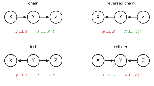
fig_17_6. Download: PDF · SVG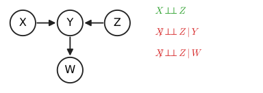
fig_17_7. Download: PDF · SVGThe rules of d-separation p. 270
- When \(Y\) is not a collider, \(X\) and \(Z\) are d-connected, but they are d-separated given \(Y\).
- If \(X\) and \(Z\) collide at \(Y\), then \(X\) and \(Z\) are d-separated, but they are d-connected given \(Y\).
- Conditioning on a descendant of a collider has the same effect as conditioning on the collider: in Figure 17.7, \(X\) and \(Z\) are d-separated but d-connected given \(W\).
Filling the gap 17.7: the three rules as statements about distributions pp. 268–270; Exercises 17.4 and 17.5
"d-connected" is a statement about the graph. What it means for distributions is: independent for every \(P\in\cM(\cG)\) when d-separated, and dependent for some (in fact almost every) \(P\in\cM(\cG)\) when d-connected.
Proofs for the four DAGs of Figure 17.6 and for Figure 17.7
Chain \(X\to Y\to Z\): \(f(x,y,z)\)
Collider \(X\to Y\leftarrow Z\): \(f(x,z)\)
Rule 3 (Figure 17.7, \(X\to Y\leftarrow Z\), \(Y\to W\)): marginally \(f(x,z)\)
The companion courses give the same three computations: Results 8.7 and 8.8, Results 11.8 and 11.9. ∎
Definition 17.B (d-separation) p. 270
Let \(X\ne Y\) be vertices and \(W\) a set of vertices containing neither. \(X\) and \(Y\) are d-separated given \(W\) if there is no undirected path \(U\) between \(X\) and \(Y\) such that (i) every collider on \(U\) has a descendant in \(W\) (the collider itself counts), and (ii) no other vertex of \(U\) is in \(W\). A path with (i) and (ii) is called active (or open) given \(W\); every other path is blocked. For disjoint sets \(A,B,W\) with \(A,B\) non-empty, \(A\) and \(B\) are d-separated given \(W\) if every \(X\in A\) and \(Y\in B\) are. Vertices or sets that are not d-separated are d-connected.
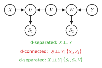
fig_17_8. Download: PDF · SVGExample 17.9. p. 270 In Figure 17.8 the only path between \(X\) and \(Y\) is \(X\to U\leftarrow V\to W\leftarrow Y\), with colliders \(U\) and \(W\) and a non-collider \(V\). Given nothing, the colliders block it: \(X\) and \(Y\) are d-separated. Given \(\{S_1,S_2\}\), both colliders have a descendant in the conditioning set and \(V\) is not in it: the path is active, \(X\) and \(Y\) are d-connected. Given \(\{S_1,S_2,V\}\), the non-collider \(V\) blocks it again.
Algorithm 17.A (d-separation by reachability, or "Bayes ball"; Geiger, Verma and Pearl, 1990; Shachter, 1998)
Definition 17.B quantifies over all paths, and their number can grow exponentially. The search below decides whether \(X\) and \(Y\) are d-separated by \(W\) in time proportional to the number of vertices plus edges. It explores states \((v,\text{direction})\): "up" if \(v\) was entered from a child (against an arrow), "down" if from a parent.
- Mark \(\an(W)\): the vertices that are in \(W\) or have a descendant in \(W\).
- Start a queue with \((X,\text{up})\). Take states from the queue, skipping any already visited:
- \((v,\text{up})\) with \(v\notin W\): add \((p,\text{up})\) for each parent \(p\) and \((c,\text{down})\) for each child \(c\);
- \((v,\text{down})\) with \(v\notin W\): add \((c,\text{down})\) for each child \(c\);
- \((v,\text{down})\) with \(v\in\an(W)\): add \((p,\text{up})\) for each parent \(p\).
- The vertices outside \(W\) that are visited are exactly those d-connected to \(X\) given \(W\); \(X\) and \(Y\) are d-separated iff \(Y\) is not visited.
Why the algorithm is correct
Call a trail a sequence of vertices, each adjacent to the next, in which vertices may repeat, and call it active if each interior occurrence passes the local test of Definition 17.B: a non-collider occurrence is not in \(W\), a collider occurrence is in \(\an(W)\). Consider an interior occurrence of \(v\) entered along edge \(e\) and left along edge \(e'\). If \(v\) was entered "up" (\(e\) leaves \(v\) by its tail), \(v\) is a non-collider whichever way \(e'\) points, so the trail may continue anywhere iff \(v\notin W\). If \(v\) was entered "down" (\(e\) points into \(v\)), leaving to a child makes \(v\) a non-collider (allowed iff \(v\notin W\)) and leaving to a parent makes it a collider (allowed iff \(v\in\an(W)\)). These are exactly the three moves of step 2, and the start state "up" lets the trail leave \(X\) in any direction. So the visited vertices are exactly the ends of active trails from \(X\). Finally, an active trail between two vertices can be shortened to an active path by cutting out the stretch between two occurrences of a repeated vertex; checking that the new occurrence still passes its test takes a short case analysis, written out in step (iii) of the proof of Result 8.9 of the companion course. Each of the at most \(2|V|\) states is expanded once along its edges, which gives the linear running time.
The code's d_separated implements the algorithm and d_separated_paths applies Definition 17.B literally by listing every path; they agree on all 3214 queries tried on the book's graphs and on 600 queries on random DAGs. ∎
See also (companion course): the same search is Algorithm 11.1 of Foundations of Deep Learning; the d-separation demo of Bayesian and Probabilistic Machine Learning lists the paths instead.
Theorem 17.10 (d-separation and conditional independence) p. 270
Let \(A,B,C\) be disjoint sets of vertices. Then \(A\indep B\given C\) if and only if \(A\) and \(B\) are d-separated by \(C\). The book assumes implicitly that \(P\) is faithful to \(\cG\): \(P\) has no independences other than those logically implied by the Markov condition.
Filling the gap 17.8: the two halves of Theorem 17.10, and faithfulness p. 270, footnote 2
The theorem has two halves of very different status.
(a) Soundness, for every \(P\in\cM(\cG)\), with no extra assumption: if \(C\) d-separates \(A\) from \(B\), then \(A\indep B\given C\). (This is the global Markov property; together with Theorem 17.6, the factorisation, the Markov condition (17.4) and the global property are three equivalent descriptions of \(\cM(\cG)\).)
(b) Completeness: if \(C\) does not d-separate \(A\) from \(B\), there is a \(P\in\cM(\cG)\) in which \(A\nindep B\given C\) (Geiger and Pearl, 1990); in fact, for discrete variables the tables for which the dependence disappears form a set of Lebesgue measure zero (Meek, 1995). So the d-separation statements are exactly the statements that hold for every \(P\in\cM(\cG)\): this set is \(\cI(\cG)\). The "only if" half of the theorem, \(A\indep B\given C\Rightarrow\) d-separation, holds for a particular \(P\) precisely when \(P\) is faithful, which is the book's assumption.
Proof of (a) in outline, and an example of (b)
(a) Let \(H=\an(A\cup B\cup C)\). By Lemma 17.C the marginal on the ancestral set \(H\) is \(\prod_{i\in H}f(x_i\given\pa_i)\). Join the parents of each common child and drop the arrow heads (the moral graph of \(H\)); each factor lives on a fully connected set of this undirected graph, and if \(C\) separates \(A\) from \(B\) in it, grouping the factors into those on the \(A\) side of \(C\) and the rest gives \(f=g(x_A,x_C)h(x_B,x_C)\) after summing out, so \(A\indep B\given C\) by Lemma 17.A. The remaining step, that d-separation in \(\cG\) implies separation in this moral graph, is a combinatorial argument about paths (Lauritzen et al., 1990), written out in full as Result 8.9(a) of the companion course.
(b), the simplest case. If an active path given \(C\) has no colliders, it has exactly one vertex \(T\) that no arrow of the path points into (an end of the path, or a fork). Let \(T\) be a fair coin, let every other vertex of the path copy its predecessor along the arrows of the path (a legitimate table, because that predecessor is one of its parents), and let all vertices off the path be independent fair coins ignoring their parents. This is a choice of tables, so \(P\in\cM(\cG)\); every variable on the path equals the same coin, while \(C\) contains no vertex of the path, so the two ends are equal and nondegenerate given \(C\): dependent. Colliders are handled by making the collider an exclusive-or of its two path neighbours and copying it down to its descendant in \(C\).
A distribution in \(\cM(\cG)\) that is not faithful. In the linear model \(Y=\alpha X+\epsilon_1\), \(Z=\beta Y+\gamma X+\epsilon_2\) (DAG \(X\to Y\to Z\), \(X\to Z\), Exercise 17.9) with independent \(\N(0,1)\) noise, \(\Cov(X,Z)=\gamma+\alpha\beta\). If \(\gamma=-\alpha\beta\) the direct and indirect effects cancel and \(X\indep Z\) (jointly Normal and uncorrelated), although \(X\) and \(Z\) are adjacent and no set d-separates them. The cancellation happens on a set of parameters of measure zero, and only for the marginal statement: the partial correlation of \(X\) and \(Z\) given \(Y\) is zero only at \(\gamma=0\) (Figure 17.S4).
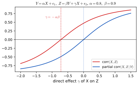
fig_17_s4. Download: PDF · SVGExample 17.11 (explaining away; Jordan, 2004). p. 271 A friend is late. Either she was abducted by aliens, or you forgot to reset your watch for daylight saving time (Figure 17.9). "Aliens" and "forgot watch" collide at "late", so they are independent: before we know she is late, there is no reason to link them. Learning that she is late raises the probability of an abduction, \(P(\text{aliens}\given\text{late})>P(\text{aliens})\); learning in addition that you forgot your watch explains the lateness and lowers it again. So the two causes are dependent given their common effect. The book gives no numbers; Figure 17.9 uses \(P(\text{aliens})=0.01\), \(P(\text{forgot})=0.1\) and \(P(\text{late}\given a,w)=0.05,0.95,0.90,0.99\) for (no, no), (yes, no), (no, yes), (yes, yes): the probability of an abduction goes from 0.0100 to 0.0666 when she is late, back down to 0.0110 if you also forgot your watch, and up to 0.1610 if you did not.
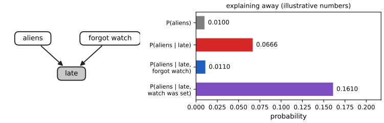
fig_17_9, aliens_probs. Download: PDF · SVGSee also (companion courses): the fuel-gauge version of explaining away, Filling the gap 8.6 and Section 11.2.2, and the explaining away demo.
Example 17.12. p. 271 In Figure 17.2, overweight and smoking are marginally independent (the only path between them has the collider "heart disease") but dependent given heart disease.
p. 271 Different-looking graphs can imply the same independences. Let \(\cI(\cG)\) be the set of independence statements implied by \(\cG\). DAGs \(\cG_1,\cG_2\) on the same variables are Markov equivalent if \(\cI(\cG_1)=\cI(\cG_2)\). The skeleton of a DAG is the undirected graph obtained by dropping the arrow heads.
Theorem 17.13 (Markov equivalence; Verma and Pearl, 1990) p. 271
Two DAGs \(\cG_1\) and \(\cG_2\) are Markov equivalent if and only if (i) \(\sk(\cG_1)=\sk(\cG_2)\) and (ii) \(\cG_1\) and \(\cG_2\) have the same unshielded colliders.
Example 17.14. p. 271 The first three DAGs of Figure 17.6 (chain, reversed chain, fork) are Markov equivalent: same skeleton, no unshielded collider. The collider is not equivalent to them.
Filling the gap 17.9: proof of Theorem 17.13, through covered edges p. 271
The book states the theorem without proof. The argument below avoids the delicate path manipulations of the original proof. "Implied by \(\cG\)" means "true for every \(P\in\cM(\cG)\)" (by Filling the gap 17.8 these are the d-separation statements).
Step 0: equivalence means equal models. \(\cI(\cG_1)=\cI(\cG_2)\) if and only if \(\cM(\cG_1)=\cM(\cG_2)\). Indeed, equal models give equal sets of statements true for all their members. Conversely, by Theorem 17.6 \(\cM(\cG_1)\) is the set of distributions satisfying the Markov statements (17.4) of \(\cG_1\); these belong to \(\cI(\cG_1)=\cI(\cG_2)\), so every \(P\in\cM(\cG_2)\) satisfies them, and \(\cM(\cG_2)\subseteq\cM(\cG_1)\); by symmetry the two are equal.
A covered edge is an arrow \(X\to Y\) with \(\pa(Y)=\pa(X)\cup\{X\}\). Reversing it keeps the model: with \(Q=\pa(X)\), the two factors \(f(x\given q)f(y\given x,q)\)
Proof of the theorem
Only if, skeletons. Suppose \(X\to Y\) in \(\cG_1\) but \(X,Y\) are not adjacent in \(\cG_2\). In \(\cG_2\) one of them, say \(X\) (otherwise rename), is not a descendant of the other; then \(Y\in\widetilde X\) and (17.4) with rule 2 gives \(X\indep Y\given\pa_{\cG_2}(X)=:S\) for every \(P\in\cM(\cG_2)\). Now choose a \(P\in\cM(\cG_1)\): all variables binary, every variable other than \(Y\) a fair coin ignoring its parents, and \(Y=X\) (a legitimate table \(f(y\given\pa_Y)=\ind\{y=x\}\), since \(X\in\pa_{\cG_1}(Y)\)). Under \(P\), \(X\) is a fair coin independent of \(S\) and \(Y=X\), so \(X\nindep Y\given S\). Hence \(\cM(\cG_1)\ne\cM(\cG_2)\).
Only if, unshielded colliders. Suppose the skeletons agree and \(X\to Y\leftarrow Z\), with \(X,Z\) not adjacent, in \(\cG_1\), while in \(\cG_2\) \(Y\) is a non-collider on \(X - Y - Z\). In \(\cG_2\) the triple is \(X\leftarrow Y\to Z\), \(X\to Y\to Z\) or \(X\leftarrow Y\leftarrow Z\). In each case there is an end, call it \(U\), with \(Y\in\pa_{\cG_2}(U)\) and the other end \(T\) not a descendant of \(U\) (for the fork take the end that is not a descendant of the other; for \(X\to Y\to Z\) take \(U=Z\), since \(X\) is an ancestor of \(Z\); symmetrically for the third). So (17.4) gives \(U\indep T\given S\) with \(S=\pa_{\cG_2}(U)\ni Y\), for every \(P\in\cM(\cG_2)\). In \(\cG_1\) choose: \(X,Z\) fair coins, \(Y=X\oplus Z\) (exclusive or), every other variable a fair coin ignoring its parents. Then \(P\in\cM(\cG_1)\), and given \(S\) (which contains \(Y\) and otherwise only independent coins) \(X\) determines \(Z\): \(X\nindep Z\given S\). Again \(\cM(\cG_1)\ne\cM(\cG_2)\).
If. Suppose \(\cG\) and \(\cH\) have the same skeleton and unshielded colliders, and let \(D\) be the set of arrows of \(\cG\) oriented the other way in \(\cH\). If \(D\ne\varnothing\), choose \(X\to Y\in D\) as follows: \(Y\) is the head of an arrow in \(D\) that comes first in a topological order of \(\cG\), and among the arrows of \(D\) into \(Y\), \(X\) is the tail that comes last. Claim: \(X\to Y\) is covered in \(\cG\).
(1) \(\pa(X)\subseteq\pa(Y)\). Let \(Z\to X\) in \(\cG\). This arrow is not in \(D\) (its head \(X\) precedes \(Y\)), so \(Z\to X\) in \(\cH\) too, where also \(Y\to X\). If \(Z\) and \(Y\) were not adjacent, \(Z\to X\leftarrow Y\) would be an unshielded collider of \(\cH\) but not of \(\cG\) (where \(X\to Y\)); so they are adjacent, and in \(\cG\) the arrow must be \(Z\to Y\) (else \(Z\to X\to Y\to Z\) is a cycle).
(2) \(\pa(Y)\subseteq\pa(X)\cup\{X\}\). Let \(W\to Y\) in \(\cG\), \(W\ne X\). If \(W\) and \(X\) were not adjacent, \(X\to Y\leftarrow W\) would be an unshielded collider of \(\cG\), hence of \(\cH\), contradicting \(Y\to X\) in \(\cH\). So they are adjacent. If \(X\to W\) in \(\cG\), then \(W\) comes after \(X\), so by the choice of \(X\) the arrow \(W\to Y\) is not in \(D\): \(W\to Y\) in \(\cH\). In \(\cH\), \(Y\to X\), so acyclicity forces \(W\to X\) there, i.e. \(X\to W\) is in \(D\) with head \(W\), which precedes \(Y\) in \(\cG\): this contradicts the choice of \(Y\). Hence \(W\to X\) in \(\cG\).
Reversing the covered edge gives a DAG (a new cycle would run \(Y\to X\leadsto Z\to Y\) with \(Z\in\pa(Y)\setminus\{X\}=\pa(X)\), so \(X\leadsto Z\to X\) would already be a cycle of \(\cG\)), with the same model (above), the same skeleton and the same unshielded colliders (by Step 0 and the "only if" part), and one arrow fewer in \(D\). After \(|D|\) reversals \(\cG\) has become \(\cH\), so \(\cM(\cG)=\cM(\cH)\). ∎
This is Chickering's (1995) transformational characterisation. The code's covered_reversal_path carries out the construction; it succeeds for all 2967 ordered pairs of equivalent DAGs on four nodes, and, by brute force over all 25 DAGs on three nodes and all 543 on four, two DAGs have the same d-separation statements exactly when they have the same skeleton and unshielded colliders (11 and 185 classes).
17.6 Estimation for DAGs
p. 272 Two questions arise: given a DAG \(\cG\) and data \(V_1,\dots,V_n\) from \(f\in\cM(\cG)\), estimate \(f\); and, given data alone, estimate \(\cG\). The first is ordinary estimation; the second is model selection. Typically one takes a parametric model \(f(x_j\given\pa_j;\th_j)\) for each conditional, and the likelihood is
\[ \mathcal L(\th)=\prod_{i=1}^{n}f(V_i;\th)=\prod_{i=1}^{n}\prod_{j=1}^{k}f(X_{ij}\given\pa_{ij};\th_j), \]where \(X_{ij}\) is the value of \(X_j\) in the \(i\)th data point and \(\pa_{ij}\) the values of its parents there.
Filling the gap 17.10: the likelihood splits into one problem per variable p. 272
If the parameters \(\th_1,\dots,\th_k\) of the different conditionals vary independently (no parameter shared between two factors), then \(\log\mathcal L(\th)=\sum_{j=1}^k\ell_j(\th_j)\) with \(\ell_j(\th_j)=\sum_i\log f(X_{ij}\given\pa_{ij};\th_j)\), so the MLE is obtained by maximising each \(\ell_j\) separately: one regression of each variable on its parents.
- Discrete variables, unrestricted tables. \(\widehat f(x_j\given\pa_j)=N(x_j,\pa_j)/N(\pa_j)\), the empirical conditional frequency, where \(N(\cdot)\) counts data points. (Each parent configuration is a separate multinomial; maximising \(\sum_xN_x\log p_x\) subject to \(\sum_xp_x=1\) gives \(p_x=N_x/\sum N\) by a Lagrange multiplier.) Plugging these in gives the maximised log-likelihood \[ \widehat\ell=\sum_j\sum_{x_j,\pa_j}N(x_j,\pa_j)\log\frac{N(x_j,\pa_j)}{N(\pa_j)} . \]
- Linear-Gaussian DAGs, \(X_j=\beta_{j0}+\sum_{p\in\pa_j}\beta_{jp}X_p+\epsilon_j\), \(\epsilon_j\sim\N(0,\sigma_j^2)\): each \(\ell_j\) is the Normal regression likelihood, so \(\widehat\beta_j\) is least squares of \(X_j\) on its parents and \(\widehat\sigma_j^2\) the mean squared residual (Result 11.4 of the companion course gives the implied joint Normal).
Standard errors come from the usual theory (the multiparameter delta method) or the bootstrap; Exercise 17.6 does both. The MLE of the joint probabilities then satisfies every independence of \(\cG\) exactly, which the unrestricted cell frequencies do not (Figure 17.S3).
p. 272 To estimate the structure one could fit every DAG by maximum likelihood and choose one by AIC or a similar criterion. The book names three obstacles: there are very many DAGs, so the search is expensive and needs much data; and an honest confidence set for the structure would need enormous samples. There is a fourth, more basic one.
Theorem 17.D (Markov equivalent DAGs fit equally well)
Let \(\cG_1\) and \(\cG_2\) be Markov equivalent DAGs on discrete variables with unrestricted conditional tables (or linear-Gaussian DAGs). For every data set, they have the same maximised likelihood and the same number of free parameters; hence the same AIC, BIC and any other criterion built from these two numbers.
Proof
The maximised likelihood is \(\sup_{P\in\cM(\cG)}\prod_if_P(V_i)\), because unrestricted tables (or all regression coefficients and variances) parametrise all of \(\cM(\cG)\) (Lemma 17.C). By Step 0 of Filling the gap 17.9, \(\cM(\cG_1)=\cM(\cG_2)\), so the suprema are equal. For the dimension, by the same proof \(\cG_1\) is turned into \(\cG_2\) by covered-edge reversals, so it suffices that a reversal keeps the count. For a covered edge \(X\to Y\) with \(Q=\pa(X)\) taking \(r_Q\) values and \(X,Y\) taking \(r_X,r_Y\) values, the two affected tables have \((r_X-1)r_Q+(r_Y-1)r_Xr_Q=r_Q(r_Xr_Y-1)\) free parameters before the reversal and \((r_Y-1)r_Q+(r_X-1)r_Yr_Q=r_Q(r_Xr_Y-1)\) after. (Linear-Gaussian: the two regressions have \(|Q|+2\) and \(|Q|+3\) parameters, intercepts and variances included, both before and after.) ∎
For simulated data on four binary variables, the maximised log-likelihoods of the 543 DAGs fall into the 185 classes with spreads below \(10^{-12}\) inside each class.
So data, however many, can at best identify the Markov equivalence class of the true DAG: the arrows that are the same throughout the class (the essential graph) are identifiable, the others are not. Remark 17.16 below returns to this for causal graphs.
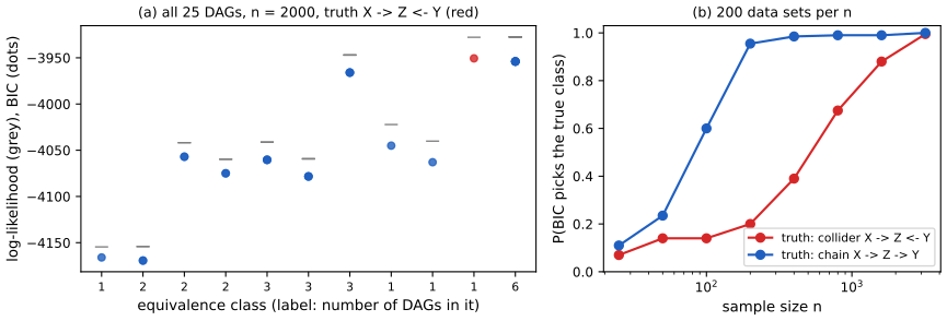
fig_17_s5. Download: PDF · SVGFilling the gap 17.11: how many DAGs? p. 272
The number \(a(k)\) of DAGs on \(k\) labelled vertices satisfies Robinson's (1973) recursion \(a(0)=1\), \(a(k)=\sum_{j=1}^k(-1)^{j+1}\binom kj2^{j(k-j)}a(k-j)\) (proof by inclusion and exclusion over the vertices without parents: Result 8.24 of the companion course), giving 1, 3, 25, 543, 29 281 and, for \(k=10\), about \(4.2\times10^{18}\). Enumeration shows 1, 2, 11, 185, 8782 Markov equivalence classes for \(k=1,\dots,5\): on average 3.3 DAGs per class at \(k=5\), approaching about 3.7 for large \(k\) (Gillispie and Perlman, 2002). Exhaustive search is hopeless beyond about six variables; practical methods search greedily over classes (Chickering, 2002) or test conditional independences one at a time (the PC algorithm, Spirtes et al., 2000).
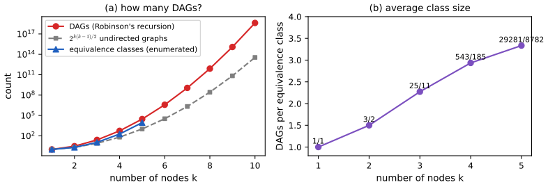
fig_17_s6. Download: PDF · SVGSee also (companion course): Bayesian structure scores, Section 8.4.8 of Bayesian and Probabilistic Machine Learning.
17.7 Bibliographic Remarks
p. 272 Texts on DAGs include Edwards (1995) and Jordan (2004). DAGs were first used to represent causal relations by Wright (1934); modern treatments are Spirtes, Glymour and Scheines (2000) and Pearl (2000). Robins, Scheines, Spirtes and Wasserman (2003) discuss why causal structure cannot be estimated uniformly consistently from data. For the proofs filled in above see Lauritzen (1996), Lauritzen, Dawid, Larsen and Leimer (1990), Verma and Pearl (1990), Geiger and Pearl (1990), Meek (1995) and Chickering (1995).
17.8 Appendix: Causation Revisited
pp. 272–274 Chapter 16 described causation with counterfactual random variables. DAGs give a second description, mathematically equivalent (Filling the gap 17.14), whose extra ingredient is the intervention. Take the DAG of Figure 17.10, \(f(x,y,z)=f(x)f(y\given x)f(z\given x,y)\), and the program that generates from it: for each run, draw \(x\) from \(f(x)\), then \(y\) from \(f(y\given x)\), then \(z\) from \(f(z\given x,y)\). Among the runs in which \(Y=y\), how often is \(Z=z\)? That is the conditional distribution:
\[ P(Z=z\given Y=y)=\frac{f(y,z)}{f(y)}=\frac{\sum_xf(x)f(y\given x)f(z\given x,y)}{f(y)}=\sum_xf(z\given x,y)\,\frac{f(x,y)}{f(y)}=\sum_xf(z\given x,y)\,f(x\given y). \]Now intervene: change the program so that \(Y\) is set to \(y\) instead of being drawn. The runs now come from \(f^*(x,z)=f(x)f(z\given x,y)\), and
\[ f^*(z)=\sum_xf(x)\,f(z\given x,y)=:P(Z=z\given Y\set y). \]\(P(Z=z\given Y=y)\) is conditioning by observation (passive), \(P(Z=z\given Y\set y)\) conditioning by intervention (active). The first answers "given that Joe smokes, how likely is lung cancer?", the second "if Joe quits smoking, how likely is lung cancer?". The two formulas differ only in the weight given to \(x\): \(f(x\given y)\) or \(f(x)\). They agree when \(f(x\given y)=f(x)\), e.g. when \(Y\) is randomised.
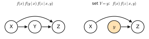
fig_17_10. Download: PDF · SVGDefinition 17.C (intervention; the truncated factorisation) p. 274
Let \(P\in\cM(\cG)\) with probability function \(f\), let \(X\) be a vertex and \(x\) a value with \(f(x\given\pa_X)>0\) for all \(\pa_X\). The intervention "set \(X=x\)" is represented by the pair \((\cG^*,f^*)\), where
- \(\cG^*\) is \(\cG\) with every arrow into \(X\) removed;
- \(f^*\) is (17.3) with the factor of \(X\) removed and \(X\) held at \(x\): for the other variables \(v'\), \[ f^*(v')=P(V'=v'\given X\set x)=\prod_{i:X_i\ne X}f(x_i\given\pa_i)\Big|_{X=x}=\frac{f(v',x)}{f(x\given\pa_X)}. \]
Theorem 17.E (what an intervention does)
(a) \(f^*\) is a probability function, Markov to \(\cG^*\) (with \(X\) a constant), and the conditionals of all variables other than \(X\) are the same as under \(f\).
(b) Intervening on \(X\) does not change the distribution of its non-descendants: for \(S\subseteq\nd(X)\), \(P(S=s\given X\set x)=P(S=s)\).
(c) If \(X\) has no parents, intervening equals conditioning: \(P(V'=v'\given X\set x)=P(V'=v'\given X=x)\).
(d) In general they differ: in Figure 17.10, \(P(Z=1\given Y\set y)\ne P(Z=1\given Y=y)\) whenever \(X\) affects both \(Y\) and \(Z\) (Exercise 17.8).
Proof
(a) The factors \(f(x_i\given\pa_i)\), \(X_i\ne X\), evaluated at \(X=x\), are conditional probability functions of \(x_i\) given the parents of \(X_i\) in \(\cG^*\) (where \(X\) is now a fixed number). Lemma 17.C applied in \(\cG^*\) shows their product is a probability function whose conditionals are these factors. The last expression in the definition is (17.3) divided by the missing factor.
(b) \(\nd(X)\) is ancestral in \(\cG\) (see the proof of Theorem 17.6) and does not contain \(X\), so it is ancestral in \(\cG^*\) too. By Lemma 17.C in \(\cG^*\), the marginal of \(f^*\) on \(\nd(X)\) is \(\prod_{i\in\nd(X)}f(x_i\given\pa_i)\), which does not involve \(x\) (no non-descendant has \(X\) as a parent); by Lemma 17.C in \(\cG\) this is also the marginal of \(f\). Marginalise further to \(S\).
(c) With no parents, \(f(x\given\pa_X)=f(x)\) and \(f^*(v')=f(v',x)/f(x)=f(v'\given x)\).
(d) is the computation above with the numbers of Exercise 17.8. ∎
Theorem 17.F (adjustment for the parents)
Under the conditions of Definition 17.C, for any variable \(Y\ne X\) outside \(\pa_X\),
\[ P(Y=y\given X\set x)=\sum_{q}P(Y=y\given X=x,\pa_X=q)\,P(\pa_X=q), \]and \(\E(Y\given X\set x)\)
Proof
Write the variables as \(X\), \(Q=\pa_X\), \(Y\) and the rest \(R\). By the definition, \(f^*(y,q,r)=f(x,y,q,r)/f(x\given q)\). Since \(f(x,y,q,r)=f(y,r\given x,q)f(x\given q)f(q)\), this is \(f(y,r\given x,q)\,f(q)\). Summing over \(r\) and \(q\): \(P(Y=y\given X\set x)=\sum_qf(y\given x,q)f(q)\). The positivity condition \(f(x\given q)>0\) ("overlap") is what makes \(f(y\given x,q)\) defined for every \(q\) that has positive probability. ∎
The parents are one valid adjustment set; any set \(S\) of non-descendants of \(X\) that blocks every path between \(X\) and \(Y\) starting with an arrow into \(X\) also works (Pearl's back-door criterion, 1993; Pearl, 2000, Section 3.3), which matters when some parents are unobserved.
See also (Chapter 16): the same formula from counterfactuals, Theorem 16.6 with its positivity condition (Filling the gap 16.6), and the sign reversal of preset 3 of the demo as Simpson's paradox.
For random tables on the observational design of Figure 17.11 (middle), the truncated factorisation computed on the joint table agrees with the adjustment formula to \(10^{-15}\), and differs from the naive \(P(Y=1\given X=1)\).
Example 17.15 (rain and wet lawn). pp. 274–275 Rain \(R\) and a wet lawn \(W\) are dependent. Both DAGs \(R\to W\) and \(R\leftarrow W\) represent the joint distribution correctly, \(f(r,w)=f(r)f(w\given r)=f(w)f(r\given w)\); they are Markov equivalent (the single arrow is a covered edge). But only the first is right causally, because only its interventions are right: in \(R\to W\), setting \(W=1\) removes nothing that \(R\) depends on, and \(P(R=r\given W\set1)=P(R=r)\) (Theorem 17.E(b)): wetting the lawn does not cause rain. In \(R\leftarrow W\), \(W\) has no parents, so \(P(R=r\given W\set1)=P(R=r\given W=1)\) (Theorem 17.E(c)), which says that wetting the lawn changes the chance of rain: nonsense. Both are correct probability models; the causal one is chosen by background knowledge.
Remark 17.16. p. 275 Learning the causal graph from data is dangerous. With two variables it is impossible: \(R\to W\) and \(R\leftarrow W\) are Markov equivalent and fit every data set equally well (Theorem 17.D). With more variables, some arrows (those of the essential graph, such as the arrows into an unshielded collider) can be learned, under assumptions such as faithfulness, but the methods are large-sample methods and there is no way to tell from the data whether the sample is large enough (Robins et al., 2003; compare the slow curve of Figure 17.S5(b)).
p. 275 DAGs also represent confounding. With treatment \(X\), outcome \(Y\) and a variable \(Z\) with arrows into both, three designs appear in Figure 17.11.
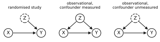
fig_17_11. Download: PDF · SVGFilling the gap 17.13: the three designs of Figure 17.11 p. 275
The book says the following facts are "easy to check"; here are the proofs.
(a) Randomised study. Randomisation removes the arrow \(Z\to X\): \(X\) has no parents. By Theorem 17.E(c), \(\E(Y\given X\set x)=\E(Y\given X=x)\), which involves only the observed \((X,Y)\), even though \(Z\) is unobserved.
(b) Observational study, confounder observed. \(\pa_X=\{Z\}\), so Theorem 17.F gives formula (16.7) of Chapter 16 (Theorem 16.6), to be compared with the association:
\[ \E(Y\given X\set x)=\int\E(Y\given X=x,Z=z)\,\d F_Z(z),\qquad \E(Y\given X=x)=\int\E(Y\given X=x,Z=z)\,\d F_{Z\given X}(z\given x). \]Association weights the strata by \(f(z\given x)\), causation by \(f(z)\).
(c) Observational study, confounder unobserved. The causal effect is not identifiable from the distribution of \((X,Y)\). Model A: \(X\) a fair coin and \(Y=X\) (no confounder). Model B: \(Z\) a fair coin, \(X=Z\), \(Y=Z\) (no arrow \(X\to Y\) at all, or an arrow with a table that ignores \(x\)). Both give the same joint law of \((X,Y)\), \(P(X=Y=0)=P(X=Y=1)=\tfrac12\), but \(P(Y=1\given X\set1)=1\) in model A and \(\tfrac12\) in model B. So no function of the \((X,Y)\) distribution can equal the causal effect in both, and \(P(Y=y\given X=x)\ne P(Y=y\given X\set x)\) in general: causation is not association.
Filling the gap 17.14: the correspondence between DAGs and counterfactuals pp. 275–276
The book defines \(Z\in\{1,2,3,4\}\) from the pair of potential outcomes \((C_0,C_1)\) of a binary treatment \(X\) and outcome \(Y\) (\(Z=1,2,3,4\) for \((0,0),(0,1),(1,0),(1,1)\)) and leaves the correspondence to the reader. Here it is.
- The DAG. \(Z\) records the unit's type: what would happen under each treatment. The observed outcome is the potential outcome of the treatment received, \(Y=C_X\) (the consistency relation of Definition 16.A), a deterministic function of \((X,Z)\): \(f(y\given x,z)=\ind\{y=c_x(z)\}\), where \(c_x(z)\) is the \(x\)-th coordinate of the pair coded by \(z\). Treatment may depend on type, \(f(x\given z)\). So the joint law is Markov to \(Z\to X\to Y\), \(Z\to Y\): the observational design of Figure 17.11 with \(Z\) unobserved.
- Interventions are counterfactual means. By Theorem 17.F, \(P(Y=1\given X\set x)\)
\({}=\sum_zf(1\given x,z)f(z)\) \({}=\sum_z\ind\{c_x(z)=1\}P(Z=z)\) \({}=P(C_x=1)\), the counterfactual mean \(\th_x\) of Definition 16.B. The causal effect \(\th_1-\th_0\) is \(P(Y=1\given X\set1)-P(Y=1\given X\set0)\). - Association. \(P(Y=1\given X=x)\)
\({}=\sum_z\ind\{c_x(z)=1\}f(z\given x)\) \({}=P(C_x=1\given X=x)\), the association of Definition 16.B. - Randomisation. Deleting the arrow \(Z\to X\) means \(X\indep Z\), i.e. \(X\indep(C_0,C_1)\): exactly the randomisation condition of Chapter 16, under which association equals causation (Theorem 16.3). The four values of \(Z\) are the four response types discussed in Filling the gap 16.1.
Conversely, any DAG model defines counterfactuals: \(C_x\) is the value \(Y\) takes when the program is run with \(X\) set to \(x\) and everything else (the other inputs and the random draws) unchanged. The intervention demo uses exactly this coupling: one uniform per run decides \(Z\) under both settings, which gives each run's pair of potential outcomes. For a random joint law of \((X,C_0,C_1)\), the truncated factorisation of the DAG reproduces \(P(C_x=1)\) to \(10^{-15}\).
Notes on the book
One slip of Chapter 17 is in the author's errata list; the other points are mine, each with the evidence.
Page 275, line −4: "since in this case. P(Y = y | X = x) ..."
The period after "case" should not be there; the sentence continues. Listed in the author's errata (first printing list).
Page 278, Exercise 17.9(b): "\(dy\)" should be "\(dz\)", and "compare to (b)" should be "compare to (a)"
The display defines \(\E(Z\given Y\set y)\) as an integral of \(z f(z\given Y\set y)\), which must be taken over \(z\); the integral over \(y\) printed would not be a function of \(y\). Part (b) is asked to be compared "to (b)", i.e. to itself; the comparison intended is with \(\E(Z\given Y=y)\) of part (a). Not in the errata lists.
Page 270, Theorem 17.10 and the definition before it
(1) The footnote assumes faithfulness for the whole theorem, but only one half needs it: "d-separated \(\Rightarrow\) independent" holds for every \(P\in\cM(\cG)\), while "independent \(\Rightarrow\) d-separated" can fail (Figure 17.S4); see Filling the gap 17.8. (2) In the definition for sets, "distinct sets of vertices" should read "disjoint sets": the definition requires \(W\) to contain neither endpoint, so \(A\), \(B\), \(W\) must not overlap. Neither point is in the errata lists.
Page 272, Section 17.6: notation in the likelihood, and the limits of AIC
In \(\prod_i\prod_jf(X_{ij}\given\pa_j;\th_j)\) the parents' values change with the data point and should carry the index \(i\) (written \(\pa_{ij}\) above), and the inner product runs to \(m\) where Section 17.4 calls the number of variables \(k\). More substantively, choosing a DAG "by AIC" cannot distinguish Markov equivalent DAGs, which always tie (Theorem 17.D); the book makes the corresponding point for causal graphs only later, in Remark 17.16. Not in the errata lists.
Page 265: "staring with X" should be "starting with X"
A typographical slip in the definition of an undirected path. Not in the errata lists.
Two remarks on scope (not errors)
Remark 17.16 says learning the causal direction between two variables is impossible. That is true for the nonparametric model, where the two directions are Markov equivalent; under additional assumptions, such as linear relations with non-Gaussian noise (Shimizu et al., 2006), the direction becomes identifiable. And in Exercise 17.5 "dependent given \(Y\)" holds for some (indeed almost every) distribution Markov to the collider, not for every one (Filling the gap 17.7).
17.9 Exercises
All nine exercises of Chapter 17 (Wasserman, 2004, pp. 276–279), restated in my own words, with complete solutions (hidden).
Exercise 17.1. Show that (17.1) and (17.2) are equivalent.
Solution
See Filling the gap 17.1: (17.1) gives (17.2) by dividing by \(f(y\given z)>0\), and (17.2) gives (17.1) by multiplying, the case \(f(y\given z)=0\) being trivial because then \(f(x,y\given z)=0\) for all \(x\).
Exercise 17.2. Prove Theorem 17.2.
Solution
See Filling the gap 17.2; the counterexample to rule 5 without positivity is in Filling the gap 17.3.
Exercise 17.3. \(X,Y,Z\) are binary with \(P(X=x,Y=y,Z=0)\) equal to 0.405, 0.045, 0.045, 0.005 for \((x,y)=(0,0),(0,1),(1,0),(1,1)\), and \(P(X=x,Y=y,Z=1)=0.125\) for all four \((x,y)\). (a) Find the conditional distribution of \((X,Y)\) given \(Z=0\) and given \(Z=1\). (b) Show \(X\indep Y\given Z\). (c) Find the distribution of \((X,Y)\). (d) Show that \(X\) and \(Y\) are dependent.
Solution
(a) \(P(Z=0)=0.5=P(Z=1)\). Given \(Z=0\) the probabilities are \(0.81, 0.09, 0.09, 0.01\); given \(Z=1\) they are all \(0.25\).
(b) Given \(Z=0\), \(P(X=0\given Z=0)=P(Y=0\given Z=0)=0.9\) and the table is the product \((0.9,0.1)\otimes(0.9,0.1)\): \(0.81=0.9^2\), \(0.09=0.9\times0.1\), \(0.01=0.1^2\). Given \(Z=1\) the table is \((0.5,0.5)\otimes(0.5,0.5)\). So (17.1) holds for both values of \(z\).
(c) Adding the two halves: \(P(X=x,Y=y)=0.53, 0.17, 0.17, 0.13\).
(d) \(P(X=0)=P(Y=0)=0.7\), and \(P(X=0)P(Y=0)=0.49\)
\({}\ne0.53\) \({}=P(X=0,Y=0)\). Mixing two independent tables with different margins creates dependence: \(Z\) is a common cause (a fork \(X\leftarrow Z\to Y\)). Exercise 17.4. For each of the three DAGs of Figure 17.6 without a collider, prove \(X\indep Z\given Y\).
Solution
Chain: \(f(x,y,z)\)
\({}=f(x)f(y\given x)f(z\given y)\) \({}=f(x,y)f(z\given y)\). Reversed chain: \(f(z)f(y\given z)f(x\given y)=f(y,z)f(x\given y)\). Fork: \(f(y)f(x\given y)f(z\given y)\). Each is a function of \((x,y)\) times a function of \((z,y)\), so Lemma 17.A gives \(X\indep Z\given Y\). (Alternatively, Theorem 17.6: in each DAG one of \(X,Z\) is a non-descendant non-parent of the other with parent set \(\{Y\}\).) Exercise 17.5. For the collider \(X\to Y\leftarrow Z\) of Figure 17.6, prove that \(X\indep Z\) and that \(X\) and \(Z\) are dependent given \(Y\).
Solution
\(f(x,z)\)
\({}=\sum_yf(x)f(z)f(y\given x,z)\) \({}=f(x)f(z)\sum_yf(y\given x,z)\) \({}=f(x)f(z)\). For the dependence, the statement is about a typical member of \(\cM(\cG)\), not every member (if \(f(y\given x,z)\) ignores \((x,z)\) there is none). Take \(X,Z\) independent fair coins and \(Y=X+Z\): \(P(X=1,Z=1\given Y=1)=0\) while \(P(X=1\given Y=1)P(Z=1\given Y=1)=\tfrac14\). More generally, for binary variables \(X\indep Z\given Y=y\) forces a polynomial equation on the table \(f(y\given x,z)\), which holds only on a set of measure zero (Filling the gap 17.8). Exercise 17.6. Let \(X,Y\in\{0,1\}\), \(Z\in\{0,1,2\}\), with a distribution Markov to \(X\to Y\to Z\). Choose such a distribution, generate 1000 observations, estimate the distribution by maximum likelihood and compare it with the truth. With \(\th_{rst}=P(X=r,Y=s,Z=t)\), use the bootstrap to get standard errors and 95 percent confidence intervals for the 12 parameters.
Solution
Model. \(P(X=1)=0.6\); \(P(Y=1\given X=0)=0.3\), \(P(Y=1\given X=1)=0.8\); \(P(Z=\cdot\given Y=0)=(0.6,0.3,0.1)\), \(P(Z=\cdot\given Y=1)=(0.2,0.3,0.5)\). Estimator. By Filling the gap 17.10 the MLE under the DAG is \(\widehat\th_{rst}\)
\({}=\widehat f(r)\widehat f(s\given r)\widehat f(t\given s)\) with empirical (conditional) frequencies. Bootstrap. \(B=2000\) resamples of the 1000 rows, the MLE recomputed on each; standard error = standard deviation of the replicates, interval = 2.5% and 97.5% percentiles (Chapter 8). Results (code: ex6_bootstrap, seed 17):\(rst\) true \(\th\) MLE se 95% interval 000 0.168 0.1836 0.0115 (0.1618, 0.2063) 001 0.084 0.0967 0.0082 (0.0810, 0.1132) 002 0.028 0.0307 0.0046 (0.0221, 0.0399) 010 0.024 0.0232 0.0027 (0.0183, 0.0289) 011 0.036 0.0315 0.0035 (0.0252, 0.0387) 012 0.060 0.0482 0.0050 (0.0387, 0.0586) 100 0.072 0.0614 0.0061 (0.0496, 0.0736) 101 0.036 0.0323 0.0039 (0.0252, 0.0404) 102 0.012 0.0103 0.0018 (0.0069, 0.0140) 110 0.096 0.1088 0.0090 (0.0916, 0.1274) 111 0.144 0.1475 0.0100 (0.1284, 0.1678) 112 0.240 0.2258 0.0123 (0.2019, 0.2502) Eleven of the twelve intervals contain the true value (\(\th_{012}=0.060\) is just outside its interval), as expected for 95% intervals; the coverage of the procedure, estimated over 60 repetitions of the whole experiment, is 0.95. The bootstrap standard errors agree with the delta-method values \[ \th_{rst}\Big\{\frac{1-a_r}{na_r}+\frac{1-b_{rs}}{n_rb_{rs}}+\frac{1-c_{st}}{n_sc_{st}}\Big\}^{1/2} \] (with \(a,b,c\) the three tables and \(n_r,n_s\) the expected counts of \(X=r\), \(Y=s\)) to within 12%. The MLE satisfies \(X\indep Z\given Y\) exactly, unlike the raw cell frequencies, which are also shown in Figure 17.S3.
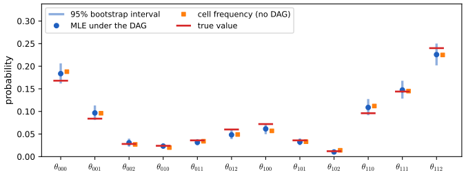
Figure 17.S3 (supplementary). Exercise 17.6: the twelve cell probabilities, their MLE under \(X\to Y\to Z\) with 95% percentile bootstrap intervals (\(B=2000\)), and the unrestricted cell frequencies. Not a figure of the book. Code: ch17_directed_graphs.py, fig_17_s3. Download: PDF · SVGExercise 17.7. For the DAG of Figure 17.12 (\(X\to Y_j\leftarrow Z_j\), \(j=1,\dots,4\)): (a) write down the factorisation of the joint density; (b) prove \(X\indep Z_j\).
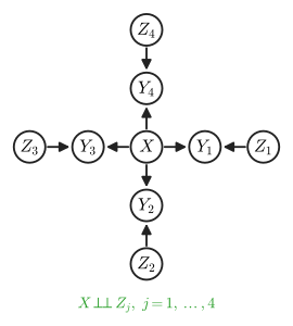
Figure 17.12. The DAG of Exercise 17.7, with the verdict \(X\indep Z_j\) computed by the reachability algorithm. Redrawn. Reproduces Wasserman (2004), Figure 17.12. Code: ch17_directed_graphs.py, fig_17_12. Download: PDF · SVGSolution
(a) \(f(x,y_1,\dots,y_4,z_1,\dots,z_4)\)
\({}=f(x)\prod_{j=1}^4f(z_j)\,f(y_j\given x,z_j)\). (b) Sum (or integrate) over all \(y_1,\dots,y_4\): each \(f(y_j\given x,z_j)\) sums to one, leaving \(f(x)\prod_jf(z_j)\); summing over the \(z_l\), \(l\ne j\), gives \(f(x,z_j)=f(x)f(z_j)\). (By d-separation: the only path between \(X\) and \(Z_j\) is \(X\to Y_j\leftarrow Z_j\), blocked at the collider \(Y_j\) when nothing is observed. Given \(Y_j\) they are dependent in general: explaining away.)
Exercise 17.8. Let \(X\sim\Bern(1/2)\), \(Y\given X=x\sim\Bern(\expit(4x-2))\) and \(Z\given X=x,Y=y\)
\({}\sim\Bern(\expit(2(x+y)-2))\). (a) Find \(P(Z=z\given Y=y)\), in particular \(P(Z=1\given Y=1)\). (b) Simulate the model and plot the empirical \(P(Z=1\given Y=1)\) against the simulation size \(N\). (c) Find \(P(Z=1\given Y\set y)\), in particular \(P(Z=1\given Y\set1)\). (d) Simulate the intervention "set \(Y=1\)" and plot the estimate of \(P(Z=1\given Y\set1)\) against \(N\). Solution
Write \(e=e^2\), so \(\expit(2)=e/(1+e)=0.8808\) and \(\expit(-2)=1/(1+e)=0.1192\). The tables: \(P(Y=1\given x)=0.1192, 0.8808\); \(P(Z=1\given x,y)=0.1192\) at \((0,0)\), \(0.5\) at \((0,1)\) and \((1,0)\), \(0.8808\) at \((1,1)\).
(a) \(P(Y=1)=\tfrac12(0.1192+0.8808)=\tfrac12\) and \(P(X=1\given Y=1)\)
\[ P(Z=1\given Y=1)=\sum_xf(1\given x,1)f(x\given1)=\Big(\frac{e}{1+e}\Big)^2+\frac12\cdot\frac{1}{1+e}=0.8354, \]\({}=\tfrac12\cdot0.8808/\tfrac12\) \({}=e/(1+e)\). By the formula of p. 273, and likewise, with \(P(X=1\given Y=0)=1/(1+e)\), \(P(Z=1\given Y=0)\)
\({}=\frac{1}{1+e}\cdot\frac{e}{1+e}+\frac12\cdot\frac{1}{1+e}\) \({}=0.1646\) (the model is symmetric under \(x\mapsto1-x\), \(y\mapsto1-y\), \(z\mapsto1-z\), so this is \(1-0.8354\)). (c) \(P(Z=1\given Y\set y)\)
\[ P(Z=1\given Y\set1)=\frac12\Big(\frac12+\frac{e}{1+e}\Big)=0.6904,\qquad P(Z=1\given Y\set0)=0.3096 . \]\({}=\sum_xf(1\given x,y)f(x)\) \({}=\tfrac12\{f(1\given0,y)+f(1\given1,y)\}\), so Observing \(Y=1\) makes \(X=1\) likely (0.881), and \(X\) itself raises \(Z\); setting \(Y=1\) leaves \(X\) a fair coin. The causal effect of \(Y\) is \(0.6904-0.3096=0.381\), the associational difference \(0.8354-0.1646=0.671\).
(b), (d) Figure 17.S1: three independent runs of each program, \(N\) up to \(10^5\). The observational estimate uses only the runs with \(Y=1\) (about half), the interventional one all runs; both settle on their own limits, which differ.
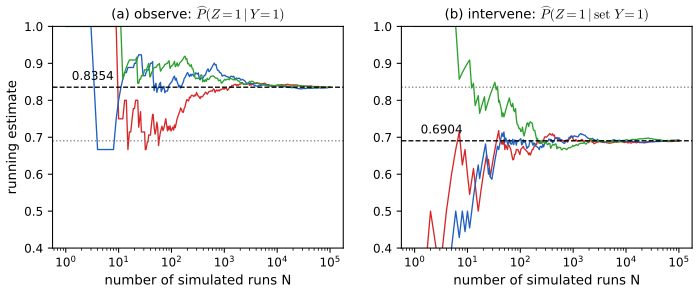
Figure 17.S1 (supplementary). Exercise 17.8 (b) and (d): running estimates from the observational program (a) and from the program with \(Y\) set to 1 (b), three runs each; dashed lines are the exact values 0.8354 and 0.6904 (each panel shows the other value dotted). Not a figure of the book. Code: ch17_directed_graphs.py, fig_17_s1. Download: PDF · SVG▶ DemoExercise 17.8 in the browserChange the strength of the confounding, the causal effect and the simulation size.Exercise 17.9 (a Gaussian structural equation model). Let \(X\sim\N(0,1)\), \(Y\given X=x\sim\N(\alpha x,1)\) and \(Z\given X=x,Y=y\)
\({}\sim\N(\beta y+\gamma x,1)\). (a) Find \(f(z\given y)\) and \(\E(Z\given Y=y)\). (b) Find \(f(z\given Y\set y)\) and \(\E(Z\given Y\set y)\); compare with (a). (c) Find the joint distribution of \((Y,Z)\) and their correlation \(\rho\). (d) Suppose \(X\) is unobserved and we declare that \(Y\) causes \(Z\) iff \(\rho\ne0\). Show that this leads to wrong conclusions. (e) In a randomised experiment, \(X\sim\N(0,1)\), \(Y\sim\N(\alpha,1)\) independently, \(Z\given X,Y\sim\N(\beta Y+\gamma X,1)\). Show that now \(\rho=0\) if and only if \(f(z\given Y\set y)\) does not depend on \(y\). Solution
Write \(Y=\alpha X+\epsilon_1\), \(Z=\beta Y+\gamma X+\epsilon_2\) with \(X,\epsilon_1,\epsilon_2\) independent \(\N(0,1)\). Then \((X,Y,Z)\) is jointly Normal with mean 0 (Result 2.16).
(a) \(\V(Y)=1+\alpha^2\), \(\Cov(X,Y)=\alpha\), so \(X\given Y=y\)
\[ f(z\given y)=\N\Big(z;\ \Big(\beta+\frac{\alpha\gamma}{1+\alpha^2}\Big)y,\ 1+\frac{\gamma^2}{1+\alpha^2}\Big),\qquad \E(Z\given Y=y)=\Big(\beta+\frac{\alpha\gamma}{1+\alpha^2}\Big)y . \]\({}\sim\N\big(\tfrac{\alpha y}{1+\alpha^2},\tfrac{1}{1+\alpha^2}\big)\). Since \(Z=\beta y+\gamma X+\epsilon_2\) given \(Y=y\), (b) Setting \(Y=y\) deletes the factor \(f(y\given x)\): \(f^*(x,z)=\phi(x)\,\phi(z-\beta y-\gamma x)\), so \(Z=\beta y+\gamma X+\epsilon_2\) with \(X\sim\N(0,1)\) and
\[ f(z\given Y\set y)=\N(z;\ \beta y,\ 1+\gamma^2),\qquad \E(Z\given Y\set y)=\beta y . \]The regression slope of (a) adds the confounding term \(\alpha\gamma/(1+\alpha^2)\) to the causal slope \(\beta\). (With \(\alpha=1\), \(\beta=0.5\), \(\gamma=-1.5\): slope \(-0.25\) against \(+0.5\); Figure 17.S2(a).)
(c) \((Y,Z)\) is bivariate Normal with mean 0, \(\V(Y)=1+\alpha^2\), \(\Cov(Y,Z)=\beta(1+\alpha^2)+\alpha\gamma\), \(\V(Z)=\beta^2(1+\alpha^2)+2\alpha\beta\gamma+\gamma^2+1\), and
\[ \rho=\frac{\beta(1+\alpha^2)+\alpha\gamma}{\sqrt{(1+\alpha^2)\big(\beta^2(1+\alpha^2)+2\alpha\beta\gamma+\gamma^2+1\big)}} . \](d) By (b), \(Y\) causes \(Z\) iff \(\beta\ne0\). But \(\rho=0\) iff \(\beta=-\alpha\gamma/(1+\alpha^2)\): if \(\alpha\gamma\ne0\), the rule declares "no effect" at this nonzero \(\beta\), and declares an effect when \(\beta=0\) (then \(\rho\propto\alpha\gamma\ne0\)). Both errors come from the unobserved common cause \(X\).
(e) Now \(\V(Y)=1\), \(\Cov(X,Y)=0\), so \(\Cov(Y,Z)=\beta\) and \(\rho=\beta/\sqrt{\beta^2+\gamma^2+1}\), which is zero iff \(\beta=0\). The intervention distribution is unchanged by how \(Y\) was assigned, \(f(z\given Y\set y)=\N(\beta y,1+\gamma^2)\), and depends on \(y\) iff \(\beta\ne0\). So under randomisation correlation detects causation (Figure 17.S2(b), blue).
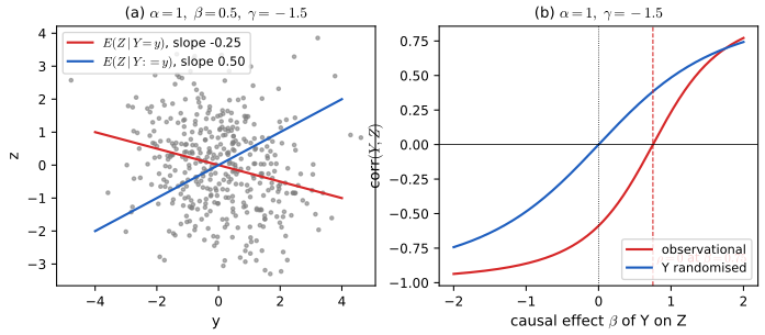
Figure 17.S2 (supplementary). Exercise 17.9 with \(\alpha=1\), \(\gamma=-1.5\). (a) Simulated data with \(\beta=0.5\): the regression of \(Z\) on \(Y\) (red) has the wrong sign; the causal line \(\E(Z\given Y\set y)=\beta y\) (blue) is not the regression line. (b) The correlation of \(Y\) and \(Z\) as the causal effect \(\beta\) varies: observationally it vanishes at \(\beta=0.75\), not at 0; with \(Y\) randomised it vanishes exactly at \(\beta=0\). Not a figure of the book. Code: ch17_directed_graphs.py, fig_17_s2. Download: PDF · SVG
Demonstrations for this chapter
Each demonstration runs in the browser and links back to these notes. The ▶ Demo boxes above open them already set to the case under discussion.
| Demonstration | What you can see | Sections and results |
|---|---|---|
| Conditioning versus intervening | The DAG \(X\to Y\to Z\), \(X\to Z\) with adjustable mechanisms; exact \(P(Z=1\given Y=y)\) and \(P(Z=1\given Y\set y)\) with the two weighting formulas; both programs simulated with running estimates. Presets: 1 Exercise 17.8; 2 association without causation; 3 a sign reversal; 4 randomised \(Y\); 5 no confounding path. | 17.8; Theorems 17.E, 17.F; Filling the gaps 17.13, 17.14; Exercise 17.8 |
| Markov equivalence | Edit a DAG on two to five binary variables; its unshielded colliders, essential graph and equivalence class; data simulated from it and every DAG on the same variables scored by AIC or BIC, one score per class. Presets: 1 a chain; 2 a collider; 3 rain and wet lawn; 4 Figure 17.3; 5 Figure 17.4. | Theorem 17.13, Filling the gap 17.9; 17.6, Theorem 17.D; Example 17.15 |
| d-separation by reachability | The reachability search step by step on the book's DAGs: visited states, reached and separated nodes, and the exact conditional mutual information under a random distribution Markov to the graph. Presets: 1–3 Example 17.9; 4 Figure 17.5; 5 Figure 17.7. | 17.5; Algorithm 17.A; Theorem 17.10; Filling the gaps 17.6, 17.8 |
Related demonstrations in the companion courses: the d-separation demo of Bayesian and Probabilistic Machine Learning, and the explaining away and linear-Gaussian DAG demos of Foundations of Deep Learning. The Python code that produces every figure of this page is code/ch17_directed_graphs.py (see the code index).
References
- Wasserman, L. (2004). All of Statistics: A Concise Course in Statistical Inference. Springer, New York. Chapter 17, pp. 263–279. www.stat.cmu.edu/~larry/all-of-statistics.
- Chickering, D. M. (1995). A transformational characterization of equivalent Bayesian network structures. In Proceedings of the Eleventh Conference on Uncertainty in Artificial Intelligence, 87–98. Morgan Kaufmann, San Francisco.
- Chickering, D. M. (2002). Optimal structure identification with greedy search. Journal of Machine Learning Research, 3, 507–554.
- Edwards, D. (1995). Introduction to Graphical Modelling. Springer, New York.
- Geiger, D. and Pearl, J. (1990). On the logic of causal models. In Uncertainty in Artificial Intelligence 4, 3–14. North-Holland, Amsterdam.
- Geiger, D., Verma, T. and Pearl, J. (1990). Identifying independence in Bayesian networks. Networks, 20(5), 507–534.
- Gillispie, S. B. and Perlman, M. D. (2002). The size distribution for Markov equivalence classes of acyclic digraph models. Artificial Intelligence, 141(1–2), 137–155.
- Jordan, M. I. (2004). Graphical models. Statistical Science, 19(1), 140–155.
- Lauritzen, S. L. (1996). Graphical Models. Oxford University Press, Oxford.
- Lauritzen, S. L., Dawid, A. P., Larsen, B. N. and Leimer, H.-G. (1990). Independence properties of directed Markov fields. Networks, 20(5), 491–505.
- Meek, C. (1995). Strong completeness and faithfulness in Bayesian networks. In Proceedings of the Eleventh Conference on Uncertainty in Artificial Intelligence, 411–418. Morgan Kaufmann, San Francisco.
- Pearl, J. (1988). Probabilistic Reasoning in Intelligent Systems. Morgan Kaufmann, San Mateo.
- Pearl, J. (1993). Comment: graphical models, causality and intervention. Statistical Science, 8(3), 266–269.
- Pearl, J. (2000). Causality: Models, Reasoning, and Inference. Cambridge University Press, Cambridge.
- Robins, J. M., Scheines, R., Spirtes, P. and Wasserman, L. (2003). Uniform consistency in causal inference. Biometrika, 90(3), 491–515.
- Robinson, R. W. (1973). Counting labeled acyclic digraphs. In New Directions in the Theory of Graphs, 239–273. Academic Press, New York.
- Shachter, R. D. (1998). Bayes-ball: the rational pastime (for determining irrelevance and requisite information in belief networks and influence diagrams). In Proceedings of the Fourteenth Conference on Uncertainty in Artificial Intelligence, 480–487. Morgan Kaufmann, San Francisco.
- Shimizu, S., Hoyer, P. O., Hyvärinen, A. and Kerminen, A. (2006). A linear non-Gaussian acyclic model for causal discovery. Journal of Machine Learning Research, 7, 2003–2030.
- Spirtes, P., Glymour, C. and Scheines, R. (2000). Causation, Prediction, and Search, 2nd edition. MIT Press, Cambridge, MA.
- Studený, M. (1992). Conditional independence relations have no finite complete characterization. In Information Theory, Statistical Decision Functions and Random Processes: Transactions of the 11th Prague Conference, Vol. B, 377–396. Kluwer, Dordrecht.
- Verma, T. and Pearl, J. (1990). Equivalence and synthesis of causal models. In Proceedings of the Sixth Conference on Uncertainty in Artificial Intelligence, 220–227. Elsevier, Amsterdam.
- Wright, S. (1934). The method of path coefficients. The Annals of Mathematical Statistics, 5(3), 161–215.
The numerical statements in the text (the rules of Theorem 17.2 and the counterexample to the last one, the Markov statements and d-separation verdicts of every figure, the agreement of the reachability algorithm with the path definition, soundness and generic completeness on random tables, the unfaithful cancellation, Theorem 17.13 by enumeration of all DAGs on three and four nodes, the counts of DAGs and equivalence classes, the covered-edge construction, the tie of equivalent DAGs in estimation, the intervention formulas, the counterfactual correspondence and the solutions of the exercises) were confirmed numerically.