Log-Linear Models
A table of counts cross-classified by several discrete variables is a multinomial sample, and a log-linear model writes the logarithm of its cell probabilities as a sum of interaction terms, one for each set of variables. Setting terms to zero expresses independence: a missing two-way interaction is a missing edge of an undirected graph, which links this chapter to the previous one. The book states the expansion, the link with conditional independence and the fitting problem briefly, and fits its example with software. These notes derive the expansion and its parameter count, prove which models a graph allows, explain why only hierarchical models are used, and work out the fitting in full: the observed margins are sufficient, the maximum likelihood estimate is the unique model table that reproduces them, and iterative proportional fitting finds it. They end with the deviance, AIC and BIC, applied to the book's breast cancer data and checked by simulation.
Ch. 1 Probability Ch. 2 Random variables Ch. 3 Expectation Ch. 4 Inequalities Ch. 5 Convergence Ch. 6 Models and inference Ch. 7 Estimating the CDF Ch. 8 Bootstrap Ch. 9 Parametric inference Ch. 10 Hypothesis testing Ch. 11 Bayesian inference Ch. 12 Decision theory Ch. 13 Regression Ch. 14 Multivariate models Ch. 15 Independence Ch. 16 Causal inference Ch. 17 Directed graphs Ch. 18 Undirected graphs Ch. 19 Log-linear models Ch. 20 Curve estimation Ch. 21 Orthogonal functions Ch. 22 Classification Ch. 23 Stochastic processes Ch. 24 Simulation
How to read these notes
They follow the book. Sections carry the book's numbers (19.1 to 19.7), and the two numbered equations keep their numbers \((19.1)\) and \((19.2)\). Numbered items keep the book's numbers (Theorem 19.1, Examples 19.2 and 19.3, Theorem 19.4, Lemma 19.5, Definition 19.6, ..., Example 19.15); results added to fill gaps are lettered (Theorem 19.A, Algorithm 19.A, Theorem 19.B). Section 19.5 gets four added subsections, because the book's text there is a page.
Filling the gaps. Wherever the book says "it can be shown", quotes a result without proof, or leaves an argument implicit, an orange Filling the gap box gives the full argument. Proofs and derivations start hidden: open one with its bar, or use the button below.
Figures and demonstrations. The five figures of the chapter are drawings of graphs; they are redrawn from their edge lists, with what can be computed from each graph and its model added. Four supplementary figures (19.S1 to 19.S4) illustrate gaps filled in the notes. All are produced by the Python code. The ▶ Demo boxes open an interactive demonstration already set to the case being discussed.
Main reference
L. Wasserman, All of Statistics: A Concise Course in Statistical Inference, Springer (2004), Chapter 19, pages 291–301 (book website: www.stat.cmu.edu/~larry/all-of-statistics). Section, equation, example and exercise numbers below refer to this book. Further reading is listed in the references.
The explanations, derivations, figures and code are my own; equations are cited by their numbers in the book.
Companion courses
Log-linear models and the tools they use appear in four companion courses on this site. The overlapping material is:
- Statistical Learning: Theory and Methods, Section 17.4 (undirected graphical models for discrete variables): Poisson log-linear models and iterative proportional fitting for binary graphical models (Result 17.15), and the no-three-way-interaction model as the pairwise model of a triangle (Filling the gap 17.2). Its Exercise 14.24 fits the independence model of a two-way table by one sweep of proportional scaling.
- Statistical Methods for Modern Biology, Section 2.5 (multinomial data) and Section 2.7.1 (two-way contingency tables and the chi-square test of independence, Filling the gap 2.10).
- Bayesian and Probabilistic Machine Learning, Result 2.23: exponential families, their moment equations for the MLE, concavity and sufficiency; Theorem 19.A below is that result for log-linear models.
- Applied Statistical Learning in R and Python, Section 4.6.2 and Result 4.7: Poisson regression, the generalised linear model that fits a log-linear model to cell counts (Filling the gap 19.10).
Within this course the chapter builds on Chapter 15 (the two-way table, Theorems 15.3 and 15.9), Chapter 18 (undirected graphs, the Hammersley-Clifford theorem 18.H and the binary interaction terms of Filling the gap 18.9, the same breast cancer data in Exercise 18.5), Wilks' theorem (Theorem 10.22) and AIC (Theorem 13.18). New here: the existence and uniqueness of the expansion for any number of levels (Filling the gap 19.1), the characterisation of graphical models by cliques (19.4), the invariance argument for hierarchy (19.5), Birch's theorem (Theorem 19.A) and a complete convergence proof for iterative proportional fitting (Theorem 19.B).
The chapter at a glance
- 19.1 Every positive probability function on a finite grid has a unique log-linear expansion \((19.1)\) into terms \(\psi_A\), one per subset of variables (Theorem 19.1). \(X_b\indep X_c\given X_a\) exactly when every term touching both \(b\) and \(c\) vanishes (Theorem 19.4).
- 19.2–19.4 A model is a list of allowed terms. It is graphical when its terms are exactly the cliques of its graph (Filling the gap 19.4), hierarchical when every sub-term of a term is allowed (Definition 19.8); graphical implies hierarchical (Lemma 19.9). Hierarchical models are written by their generators, e.g. \(1.2+2.3\).
- 19.5 The generator margins are sufficient, and the MLE is the unique table in the model with the observed generator margins (Theorem 19.A); iterative proportional fitting computes it (Algorithm 19.A, Theorem 19.B). The deviance tests a model against the saturated one with \(N-|M|\) degrees of freedom (Theorem 19.14); AIC \((19.2)\) ranks models. On the breast cancer data the selected model is \(1.2+2.3\): centre and survival are independent given grade (Example 19.15).
Notation. \(X=(X_1,\dots,X_m)\) with \(X_j\in\{0,1,\dots,r_j-1\}\); \(S=\{1,\dots,m\}\); \(\Xc=\prod_j\{0,\dots,r_j-1\}\) has \(N=r_1\cdots r_m\) cells. For \(A\subseteq S\), \(x_A=(x_j:j\in A)\), and \((x_A,0)\) is the point that agrees with \(x\) on \(A\) and is 0 elsewhere. For a table \(t\) (counts or fitted values), \(t_A(x_A)=\sum_{y:\,y_A=x_A}t(y)\) is its \(A\)-margin. \(n(x)\) are the observed counts, \(n=\sum_xn(x)\). \(f\) is positive if \(f(x)>0\) for every \(x\in\Xc\). Terms are written by their index sets: \(\psi_{12}\) is \(\psi_{\{1,2\}}\).
Prerequisites. Conditional independence and its factorisation criterion (Definition 18.C), undirected graphs and cliques (Definition 18.G), the multinomial MLE (Theorem 15.3), Fisher information for several parameters (Theorem 9.27), Wilks' theorem (Theorem 10.22). See the course home.
19.1 The Log-Linear Model
p. 291 Let \(X=(X_1,\dots,X_m)\) be discrete with probability function \(f(x)=\P(X=x)\). With \(n\) independent copies, the counts \(n(x)\) of the \(N\) cells form one multinomial sample with parameter \(p=(f(x):x\in\Xc)\), a point of the \((N-1)\)-dimensional simplex. A log-linear model re-expresses \(p\) through interaction terms.
Theorem 19.1 (the log-linear expansion) p. 292
Let \(f\) be positive. Then
\[ \log f(x)=\sum_{A\subseteq S}\psi_A(x) \tag{19.1} \]for functions \(\psi_A\) such that (1) \(\psi_\emptyset\) is a constant; (2) \(\psi_A(x)\) depends on \(x\) only through \(x_A\); (3) \(\psi_A(x)=0\) whenever \(x_i=0\) for some \(i\in A\). The functions are unique, and given by Möbius inversion:
\[ \psi_A(x)=\sum_{B\subseteq A}(-1)^{|A\setminus B|}\log f(x_B,0). \]Each \(\psi_A\) is determined by the numbers \(\beta_A(x_A)=\psi_A(x)\) at the \(\prod_{j\in A}(r_j-1)\) points with every \(x_j\ne0\), \(j\in A\): the log-linear parameters. Their total number is \(N\), and normalisation leaves \(N-1\) free.
Filling the gap 19.1: existence, uniqueness, and why \(f\) must be positive p. 292
The book states the expansion without proof and without the positivity assumption, which is needed for \(\log f\) to be defined (a table with an empty cell has no expansion; see the notes on the book). The proof below is the general version, for any numbers of levels, of the binary argument in Filling the gap 18.9.
Proof of Theorem 19.1
Write \(g_B(x)=\log f(x_B,0)\) for \(B\subseteq S\), and define \(\psi_A\) by the displayed formula.
(1) and (2). \(\psi_\emptyset=g_\emptyset=\log f(0)\) is a constant, and every \(g_B\) with \(B\subseteq A\) depends only on \(x_B\), hence on \(x_A\).
(3). Let \(i\in A\) with \(x_i=0\). Split the subsets of \(A\) into pairs \(\{B,\,B\cup\{i\}\}\) with \(B\subseteq A\setminus\{i\}\). Since \(x_i=0\), the points \((x_B,0)\) and \((x_{B\cup\{i\}},0)\) coincide, so \(g_B(x)=g_{B\cup\{i\}}(x)\), while their signs \((-1)^{|A\setminus B|}\) differ. Every pair cancels and \(\psi_A(x)=0\).
The sum is \(\log f\). Exchanging the order of summation,
\[ \sum_{A\subseteq S}\psi_A(x)=\sum_{B\subseteq S}g_B(x)\sum_{A:\,B\subseteq A\subseteq S}(-1)^{|A\setminus B|}=\sum_{B\subseteq S}g_B(x)\,(1-1)^{|S\setminus B|}, \]by the binomial theorem; the inner factor is 0 unless \(B=S\), when it is 1. So the sum is \(g_S(x)=\log f(x)\).
Uniqueness. Suppose two families satisfy (1)–(3) and both sum to \(\log f\); their differences \(\delta_A\) satisfy (1)–(3) and \(\sum_A\delta_A\equiv0\). We show \(\delta_A\equiv0\) by induction on \(|A|\). At \(x=0\) every \(\delta_A\) with \(A\ne\emptyset\) vanishes by (3), so \(\delta_\emptyset=0\). Suppose \(\delta_B\equiv0\) for all \(|B|<k\), and let \(|A|=k\). If some \(x_i=0\) with \(i\in A\), then \(\delta_A(x)=0\) by (3). Otherwise evaluate \(\sum_B\delta_B=0\) at the point \((x_A,0)\): terms with \(B\not\subseteq A\) contain an index where this point is 0 and vanish by (3); terms with \(B\subsetneq A\) vanish by the induction hypothesis. What remains is \(\delta_A(x_A)=0\). ∎
A useful corollary. If a function \(F\) on \(\Xc\) does not depend on \(x_j\), then every term of its expansion with \(j\in A\) vanishes: in the Möbius sum, pair \(B\) with \(B\cup\{j\}\) as in (3), and the two values of \(F\) coincide because \(F\) ignores \(x_j\). The proof used nothing about \(F\) being a log-probability, so the expansion of any function is unique and linear in the function.
Filling the gap 19.2: counting parameters, the surface \(\Theta\), and other identifying constraints p. 292
Count. Condition (3) leaves \(\psi_A\) free only at the points of \(\prod_{j\in A}\{1,\dots,r_j-1\}\), so \(d_A=\prod_{j\in A}(r_j-1)\) numbers per term, and
\[ \sum_{A\subseteq S}\prod_{j\in A}(r_j-1)=\prod_{j=1}^m\big(1+(r_j-1)\big)=N . \]The surface. For any real values of the \(N-1\) parameters with \(A\ne\emptyset\), the function \(h=\sum_{A\ne\emptyset}\psi_A\) is a log-probability after adding the unique constant \(\psi_\emptyset=-\log\sum_x e^{h(x)}\). So \(\Theta\) is the graph of a smooth function of \(N-1\) free coordinates: the \((N-1)\)-dimensional surface of the book, in one-to-one smooth correspondence with the open simplex (both maps \(p\mapsto\beta\) and \(\beta\mapsto p\) are explicit and smooth).
Binary variables. If every \(r_j=2\), each term has one parameter, \(\psi_A(x)=\beta_A\prod_{j\in A}x_j\). For a \(2\times2\) table, \(\beta_{12}=\log\{p_{11}p_{00}/(p_{10}p_{01})\}\) is the log odds ratio of Definition 15.1; for a \(2\times2\times2\) table, \(\beta_{123}\) is the log of the ratio of the conditional odds ratios of \((X_1,X_2)\) at \(X_3=1\) and at \(X_3=0\), so \(\beta_{123}=0\) says the 1-2 association is the same at both levels of \(X_3\).
Other constraints. Condition (3) is the "corner point" (or treatment-contrast) choice, the default of R's glm, which is how the book's tables in Example 19.15 were produced. The classical alternative (Bishop, Fienberg and Holland, 1975) asks each \(\psi_A\) to sum to zero over each of its arguments. The individual terms then change, but for hierarchical models (Filling the gap 19.5) the set of distributions in a model does not; the code confirms numerically that the two codings of the independence model of a \(3\times4\) table span the same space.
Example 19.2 (one Bernoulli variable). pp. 292–293 For \(X\sim\mathrm{Bernoulli}(p)\), \(\log f(x)=\log(1-p)+x\log\{p/(1-p)\}\): \(\psi_\emptyset=\beta_0=\log(1-p)\) and \(\psi_1(x)=\beta_1x\) with \(\beta_1=\log\{p/(1-p)\}\), the log odds. Here \(N=2\) and \(\Theta\) is the curve \(e^{\beta_0+\beta_1}+e^{\beta_0}=1\), i.e. \(\beta_0=-\log(1+e^{\beta_1})\): one free parameter.
Example 19.3 (a \(2\times3\) table). pp. 293–294 With \(X_1\in\{0,1\}\), \(X_2\in\{0,1,2\}\) and cell probabilities \(p_{ij}\), the Möbius formula gives \(\psi_\emptyset=\log p_{00}\), \(\psi_1(x)=x_1\log(p_{10}/p_{00})\),
\[ \psi_2(x)=\ind(x_2=1)\log\frac{p_{01}}{p_{00}}+\ind(x_2=2)\log\frac{p_{02}}{p_{00}},\qquad \psi_{12}(x)=\sum_{k=1}^2\ind(x_1=1,x_2=k)\log\frac{p_{1k}\,p_{00}}{p_{0k}\,p_{10}} , \]six parameters \(\beta_1,\dots,\beta_6\) in the book's numbering (\(1+1+2+2=6=N\)), of which five are free; \(\psi_{12}\) consists of the two log odds ratios of columns 1 and 2 against column 0. The inverse map is Exercise 19.1, and the code confirms both directions on a random table.
Theorem 19.4 (zero terms and conditional independence) p. 294
Let \(f\) be positive and let \((a,b,c)\) partition \(S\) (\(a\) may be empty). Then \(X_b\indep X_c\given X_a\) if and only if \(\psi_t\equiv0\) for every \(t\) that contains at least one index of \(b\) and at least one of \(c\).
Lemma 19.5 (factorisation criterion) p. 294
\(X_b\indep X_c\given X_a\) if and only if \(f(x_a,x_b,x_c)=g(x_a,x_b)\,h(x_a,x_c)\) for some nonnegative functions \(g,h\) (positivity is not needed here).
Filling the gap 19.3: proofs of Lemma 19.5 and of both directions of Theorem 19.4 p. 294; Exercise 19.2
The book proves one direction of Theorem 19.4 and says "the converse follows by reversing the argument"; the converse actually needs the uniqueness of the expansion. Its proof also contains a slip ("or" for "and", see the notes on the book).
Proof of Lemma 19.5 (Exercise 19.2)
(\(\Rightarrow\)) Put \(g(x_a,x_b)=f(x_a,x_b)\) and \(h(x_a,x_c)=f(x_c\given x_a)=f(x_a,x_c)/f(x_a)\) when \(f(x_a)>0\), and \(h=0\) otherwise. If \(f(x_a)=0\), both sides are 0. If \(f(x_a)>0\), conditional independence gives \(f(x_a,x_b,x_c)=f(x_a)f(x_b\given x_a)f(x_c\given x_a)=g\,h\).
(\(\Leftarrow\)) Let \(G(x_a)=\sum_{x_b}g(x_a,x_b)\) and \(H(x_a)=\sum_{x_c}h(x_a,x_c)\). Summing \(f=gh\) gives \(f(x_a,x_b)=g\,H\), \(f(x_a,x_c)=h\,G\) and \(f(x_a)=G\,H\). For \(f(x_a)>0\) (so \(G,H>0\)),
\[ f(x_b,x_c\given x_a)=\frac{g\,h}{G\,H}=\frac{gH}{GH}\cdot\frac{hG}{GH}=f(x_b\given x_a)\,f(x_c\given x_a). \ \ \text{∎} \]Proof of Theorem 19.4
(\(\Leftarrow\)) Suppose every term meeting both \(b\) and \(c\) is zero. Let \(\mathcal T_b\) be the sets \(t\) that meet \(b\); a nonzero term with \(t\in\mathcal T_b\) does not meet \(c\), so \(t\subseteq a\cup b\); a term with \(t\notin\mathcal T_b\) satisfies \(t\subseteq a\cup c\). Hence
\[ \log f(x)=\underbrace{\sum_{t\in\mathcal T_b}\psi_t(x)}_{\text{function of }(x_a,x_b)}+\underbrace{\sum_{t\notin\mathcal T_b}\psi_t(x)}_{\text{function of }(x_a,x_c)} , \]and exponentiating gives \(f=g\,h\), so \(X_b\indep X_c\given X_a\) by Lemma 19.5. (The book's three sums, over \(t\subseteq a\cup b\), over \(t\subseteq a\cup c\), minus over \(t\subseteq a\), group the same terms.)
(\(\Rightarrow\)) Suppose \(X_b\indep X_c\given X_a\). By Lemma 19.5 and positivity, \(f=g\,h\) with \(g=f(x_a,x_b)>0\) and \(h=f(x_c\given x_a)>0\), so \(\log f=\log g+\log h\). Expand \(\log g\) and \(\log h\) by the Möbius formula (Filling the gap 19.1 applies to any function). Since \(\log g\) does not depend on \(x_c\), its terms vanish for every \(t\) meeting \(c\) (the corollary of Filling the gap 19.1); likewise the terms of \(\log h\) vanish for every \(t\) meeting \(b\). The sum of the two expansions satisfies (1)–(3) and adds up to \(\log f\), so by uniqueness it is the expansion of \(\log f\). A set \(t\) meeting both \(b\) and \(c\) gets zero from both, so \(\psi_t\equiv0\). ∎
Numerically: for \(f=g(x_1,x_2)h(x_1,x_3)\) with random positive \(g,h\) on a \(2\times3\times2\) grid, \(\psi_{23}\) and \(\psi_{123}\) vanish to \(10^{-12}\); for a four-variable example with \(b=\{2,3\}\), \(c=\{4\}\), all six terms meeting both are zero.
19.2 Graphical Log-Linear Models
p. 294 A log-linear model is a family of distributions defined by declaring some terms \(\psi_A\) identically zero and leaving the others free. Write \(M\) for the set of free terms (always containing \(\emptyset\)). The graph of \(M\), \(\Gc(M)\), has an edge \(i-j\) whenever some \(A\in M\) contains both \(i\) and \(j\). By Theorem 19.4 with \(a=S\setminus\{i,j\}\), a missing edge means \(X_i\indep X_j\given\) rest for every distribution in the model.
Definition 19.6 (graphical model) p. 294
\(M\) is graphical (for the graph \(\Gc\)) if the terms set to zero are exactly those whose index set contains a pair \(\{i,j\}\) that is not an edge of \(\Gc\): \(A\notin M\iff A\) contains a non-adjacent pair.
Filling the gap 19.4: a model is graphical exactly when its terms are the cliques of its graph pp. 294–296
A set \(A\) contains no non-adjacent pair exactly when \(A\) is complete (a clique, not necessarily maximal, including \(\emptyset\) and the single vertices). So Definition 19.6 says:
\[ M\text{ is graphical for }\Gc\iff M=\{A\subseteq S:\ A\text{ is complete in }\Gc\}. \]Three consequences.
- The graph is then \(\Gc(M)\). Every edge \(\{i,j\}\) of \(\Gc\) is complete, so it is a term of \(M\); conversely a pair inside a term of \(M\) is an edge. Hence a model is graphical if and only if \(M\) equals the set of complete sets of its own graph \(\Gc(M)\). This is the book's rule of thumb made precise: if a term can be added without changing the graph, that term is complete in \(\Gc(M)\) and missing from \(M\), so \(M\) is not graphical.
- Generators are the maximal cliques. Every complete set lies in a maximal clique, and every subset of a clique is complete. So the graphical model of \(\Gc\) consists of all subsets of the maximal cliques: in the notation of Section 19.4, its generator is the list of maximal cliques (isolated vertices included).
- The link with Chapter 18. A positive \(f\) belongs to the graphical model of \(\Gc\) if and only if \(f\) is Markov to \(\Gc\). One direction is Theorem 19.4 applied to each non-edge (the pairwise property, which for positive \(f\) gives the global property, Theorem 18.3). Conversely, if \(f\) is pairwise Markov, Theorem 19.4 removes every term containing a non-adjacent pair, which is the Hammersley-Clifford theorem in log-linear form (Theorem 18.H, Filling the gap 18.9). So the graphical log-linear model is the set of positive distributions with the graph's independence structure, and nothing more.
The code checks the characterisation on all \(2^6=64\) graphs on four vertices: each set of complete sets is a graphical, hierarchical model whose graph is the given one and which is generated by the maximal cliques.
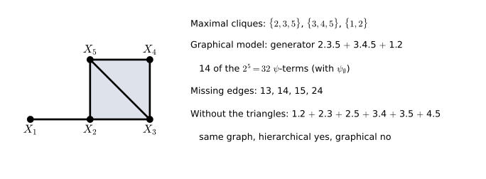
fig_19_1. Download: PDF · SVGExample 19.7. p. 295 The maximal cliques of Figure 19.1 are \(\{1,2\}\), \(\{2,3,5\}\) and \(\{3,4,5\}\), so the graphical model is
\[ \log f=\psi_\emptyset+\sum_{j=1}^5\psi_j+\psi_{12}+\psi_{23}+\psi_{25}+\psi_{34}+\psi_{35}+\psi_{45}+\psi_{235}+\psi_{345}, \]14 of the \(2^5=32\) terms. Each missing edge removes every term containing it: the 8 terms containing \(\{1,5\}\) and the 8 containing \(\{2,4\}\) listed by the book, and also those containing \(\{1,3\}\) or \(\{1,4\}\). Dropping \(\psi_{235}\) and \(\psi_{345}\) leaves a model with the same graph, hence the same conditional independences, but an extra constraint: without \(\psi_{235}\), the association between \(X_2\) and \(X_3\) (measured by their log odds ratios given the other variables) does not change with \(X_5\). That model is hierarchical but not graphical.
19.3 Hierarchical Log-Linear Models
Definition 19.8 (hierarchical model) p. 296
\(M\) is hierarchical if \(A\in M\) and \(B\subseteq A\) imply \(B\in M\); equivalently, if \(\psi_A\equiv0\) and \(A\subseteq B\) imply \(\psi_B\equiv0\).
Lemma 19.9 p. 296
Every graphical model is hierarchical; the converse is false.
Filling the gap 19.5: proof of Lemma 19.9, why models should be hierarchical, and how many there are p. 296; Exercise 19.3
Proof of Lemma 19.9 (Exercise 19.3)
Let \(M\) be graphical for \(\Gc\), \(A\in M\) and \(B\subseteq A\). \(A\) is complete, so every pair in \(B\) is an edge, so \(B\) is complete and \(B\in M\). For the converse, Example 19.11 below (\(1.2+1.3+2.3\)) is hierarchical, its graph is the triangle, and the complete set \(\{1,2,3\}\) is missing, so it is not graphical. ∎
Why hierarchical? The book says non-hierarchical models are "less interpretable". There is a sharper reason: they depend on the arbitrary choice of which level of each variable is called 0.
Hierarchical models do not depend on the coding; others do
For a set \(M\) of terms let \(V_M\) be the set of functions \(\sum_{A\in M}\psi_A\) with each \(\psi_A\) satisfying (2) and (3); the model is \(\{f:\log f\in V_M\}\). Let \(F_A\) be the space of all functions of \(x_A\). If \(M\) is hierarchical, \(V_M=\sum_{A\in M}F_A\). Indeed \(\subseteq\) is clear; for \(\supseteq\), the expansion of any \(F\in F_A\) (Filling the gap 19.1) has terms only on subsets of \(A\), which are in \(M\). The space \(\sum_{A\in M}F_A\) makes no reference to a reference level, so relabelling the levels of any variable (or using sum-to-zero constraints) gives the same model.
For a non-hierarchical model this fails. Take \(\psi_\emptyset+\psi_3+\psi_{12}\) with \(r_1=3\): \(\psi_{12}\) must vanish when \(x_1=0\), so which level is labelled 0 matters, and the code confirms that relabelling the levels of \(X_1\) changes the set of distributions (the two design matrices span different spaces). A statement such as "\(\psi_1=0\) but \(\psi_{12}\ne0\)" is a statement about the coding, not about the data.
How many models? Hierarchical models on \(m\) variables are the families of subsets closed under taking subsets; graphical ones correspond one to one with graphs. Counted by the code:
| \(m\) | hierarchical | hierarchical with all main effects | graphical |
|---|---|---|---|
| 3 | 19 | 9 | 8 |
| 4 | 167 | 114 | 64 |
(The hierarchical counts are the Dedekind numbers minus one: 20 and 168 families closed under subsets, minus the empty family.) With three variables and all main effects there is exactly one hierarchical model that is not graphical: no three-way interaction, \(1.2+1.3+2.3\). Restricting a search to graphical or hierarchical models therefore cuts the search space drastically, as the book notes in Section 19.5.
Example 19.10. p. 296 \(\log f=\psi_\emptyset+\psi_1+\psi_2+\psi_3+\psi_{12}+\psi_{13}\) (generator \(1.2+1.3\)) has the graph \(X_2-X_1-X_3\) of Figure 19.2. Its terms are exactly the cliques of that graph, so it is graphical, and by Theorem 19.4 \(X_2\indep X_3\given X_1\).
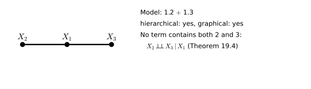
fig_19_2. Download: PDF · SVGExample 19.11. pp. 296–297 \(\log f=\psi_\emptyset+\psi_1+\psi_2+\psi_3+\psi_{12}+\psi_{13}+\psi_{23}\): hierarchical, with the complete graph of Figure 19.3, but not graphical since the clique \(\{1,2,3\}\) is missing. The constraint \(\psi_{123}=0\) is not a conditional independence: for binary variables it says the odds ratio of \((X_1,X_2)\) is the same at both levels of \(X_3\) (Filling the gap 19.2).
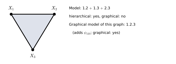
fig_19_3. Download: PDF · SVGExample 19.12. p. 297 \(\log f=\psi_\emptyset+\psi_3+\psi_{12}\) is not hierarchical (\(\psi_{12}\) without \(\psi_1\), \(\psi_2\)), hence not graphical by Lemma 19.9. Its graph is in Figure 19.4; its hierarchical closure is \(1.2+3\).
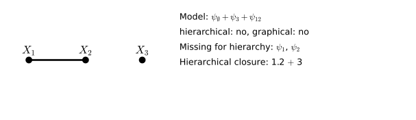
fig_19_4. Download: PDF · SVG19.4 Model Generators
pp. 297–298 A hierarchical model is determined by its maximal terms, the generators, written with dots inside a term and plus signs between terms: \(M=1.2+1.3\) means \(\psi_{12}\), \(\psi_{13}\) and all their sub-terms. The saturated model of three variables is \(1.2.3\); \(1+2+3\) is mutual independence; \(1.2\) is \(\psi_\emptyset+\psi_1+\psi_2+\psi_{12}\).
Filling the gap 19.6: what the generators of a three-way table mean, and their MLEs pp. 297–298
Each claim of Section 19.4 follows from Theorem 19.4 and uniqueness; the table lists all hierarchical models of a three-way table that keep the main effects (up to relabelling), with the MLE of the fitted counts \(\hat m=n\hat p\) derived in Filling the gap 19.9. Write \(n_{ij+}=\sum_kn_{ijk}\) and so on.
| generator | \(|M|\) (binary) | meaning | \(\hat m_{ijk}\) |
|---|---|---|---|
| \(1+2+3\) | 4 | mutual independence | \(n_{i++}n_{+j+}n_{++k}/n^2\) |
| \(1.2+3\) | 5 | \(X_3\indep(X_1,X_2)\) | \(n_{ij+}n_{++k}/n\) |
| \(1.2+2.3\) | 6 | \(X_1\indep X_3\given X_2\) | \(n_{ij+}n_{+jk}/n_{+j+}\) |
| \(1.2+1.3+2.3\) | 7 | no three-way interaction (not an independence) | no closed form |
| \(1.2.3\) | 8 | saturated: any positive multinomial | \(n_{ijk}\) |
Derivations
Saturated. All \(N\) parameters are free, so by Filling the gap 19.2 every positive \(p\) is in the model: the saturated model is the unrestricted multinomial (on the open simplex).
\(1+2+3\). \(\log f=\psi_\emptyset+\psi_1(x_1)+\psi_2(x_2)+\psi_3(x_3)\) exponentiates to a product of functions of one variable each, so \(f(x)=f_1(x_1)f_2(x_2)f_3(x_3)\) (sum out two variables to identify the factors). Conversely, if the variables are independent, \(\log f=\sum_j\log f_j(x_j)\), and by uniqueness its expansion has no interaction terms.
\(1.2+3\). Theorem 19.4 with \(a=\emptyset\), \(b=\{1,2\}\), \(c=\{3\}\): no term meets both, so \(X_3\indep(X_1,X_2)\).
\(1.2\). No term contains 3, so \(f(x)\) does not depend on \(x_3\); summing over the \(r_3\) values gives \(f(x_1,x_2)=r_3f(x)\), so \(f(x_3\given x_1,x_2)=1/r_3\): uniform, as the book says, and also independent of \((X_1,X_2)\). Such models (missing a main effect) are hierarchical but rarely sensible, which is why searches keep all main effects.
\(1.2+2.3\). No term meets both 1 and 3; Theorem 19.4 with \(a=\{2\}\) gives \(X_1\indep X_3\given X_2\).
19.5 Fitting Log-Linear Models to Data
p. 298 For a model \(M\) with parameters \(\beta\), the log-likelihood of \(n\) observations is \(\ell(\beta)=\sum_{i=1}^n\log f(X_i;\beta)=\sum_xn(x)\log f(x;\beta)\). The book says the MLE "generally has to be found numerically". The subsections below show what is special about this likelihood: it depends on the data only through margins, its maximiser is characterised by them, and a simple algorithm finds it; for many models it even has a closed form.
19.5.1 The MLE and its sufficient margins (added)
Theorem 19.A (sufficient margins; Birch, 1963)
Let \(M\) be hierarchical with generators \(C_1,\dots,C_k\). (a) The log-likelihood depends on the data only through the observed margins \(n_{C_1},\dots,n_{C_k}\), which are therefore sufficient. (b) If a positive table \(\hat m\) satisfies \(\log\hat m\in V_M\) (it is in the model) and
\[ \hat m_{C_j}=n_{C_j}\qquad(j=1,\dots,k), \]then \(\hat p=\hat m/n\) is the MLE, and it is the only one. (c) If every \(n(x)>0\), the MLE exists.
Filling the gap 19.7: proof of Theorem 19.A p. 298
This is the exponential-family structure of log-linear models (Result 2.23 of a companion course, Filling the gap 9.22 here): the sufficient statistics are the margins, and the MLE matches their expected values to the observed ones.
Proof
(a) For \(A\in M\), \(A\subseteq C_j\) for some generator, and \(\sum_xn(x)\psi_A(x)=\sum_{x_A}n_A(x_A)\psi_A(x_A)\), where \(n_A\) is a margin of \(n_{C_j}\). So \(\ell=\sum_{A\in M}\sum_{x_A}n_A\psi_A\) is a function of the generator margins and the parameters.
A Poisson reformulation. Consider \(L(\mu)=\sum_x\{n(x)\log\mu(x)-\mu(x)\}\) over tables \(\mu>0\) with \(\theta=\log\mu\in V_M\). Because \(V_M\) contains the constants, any such \(\mu\) can be written \(\mu=s\,p\) with \(s=\sum\mu\) and \(p\) in the model, and \(L=\sum_xn(x)\log p(x)+n\log s-s\). For fixed \(p\) this is maximised at \(s=n\). So maximising \(L\) over \(V_M\) and maximising the multinomial \(\ell\) over the model give the same \(\hat p=\hat\mu/n\), with \(\sum\hat\mu=n\).
(b) As a function of \(\theta\in V_M\), \(L=\sum_x\{n(x)\theta(x)-e^{\theta(x)}\}\) is strictly concave (each \(-e^{\theta(x)}\) is strictly concave in the coordinate \(\theta(x)\)). Its derivative in a direction \(v\in V_M\) is \(\sum_x\{n(x)-\mu(x)\}v(x)\). By Filling the gap 19.5, \(V_M=\sum_jF_{C_j}\) is spanned by the indicators \(v(x)=\ind(x_{C_j}=c)\), and for these the derivative is \(n_{C_j}(c)-\mu_{C_j}(c)\). So \(\theta\) is a stationary point exactly when all generator margins match. A stationary point of a concave function is a global maximum, and strict concavity makes it unique.
(c) If every \(n(x)>0\), each summand \(n(x)\theta(x)-e^{\theta(x)}\) is at most \(n(x)\log n(x)-n(x)\) and tends to \(-\infty\) as \(|\theta(x)|\to\infty\). Hence \(\{\theta\in V_M:L(\theta)\ge L(0)\}\) is closed and bounded, and the continuous \(L\) attains its maximum there. ∎
With empty cells the MLE may fail to exist even when every margin is positive; the exact condition (the observed margins lie in the relative interior of the set of achievable margins) is due to Haberman (1974). Filling the gap 19.8 gives an example.
19.5.2 Iterative proportional fitting (added)
Algorithm 19.A (iterative proportional fitting; Deming and Stephan, 1940)
- Start from a table in the model with total \(n\), e.g. \(m^{(0)}(x)=n/N\).
- For \(t=1,2,\dots\), take the next generator \(C\) in cyclic order and rescale so that its margin is right: \[ m^{(t)}(x)=m^{(t-1)}(x)\,\frac{n_C(x_C)}{m^{(t-1)}_C(x_C)} . \]
- Stop when every generator margin of \(m^{(t)}\) is within a tolerance of the observed one.
Theorem 19.B (convergence of iterative proportional fitting)
If every \(n(x)>0\), the tables \(m^{(t)}\) of Algorithm 19.A stay in the model, their multinomial log-likelihood \(\ell(m)=\sum_xn(x)\log\{m(x)/n\}\) never decreases, and \(m^{(t)}\to\hat m\), the MLE of Theorem 19.A.
Filling the gap 19.8: proof of Theorem 19.B, the starting table, and what zeros do p. 298
Proof of Theorem 19.B
Step 1: the iterates stay in the model. \(\log m^{(t)}=\log m^{(t-1)}+\log\{n_C/m^{(t-1)}_C\}(x_C)\), and the added function of \(x_C\) is in \(F_C\subseteq V_M\). Summing the update over the cells with \(x_C=c\) gives \(m^{(t)}_C=n_C\), so the total stays \(n\).
Step 2: each step raises \(\ell\) by a Kullback-Leibler divergence.
\[ \ell(m^{(t)})-\ell(m^{(t-1)})=\sum_xn(x)\log\frac{n_C(x_C)}{m^{(t-1)}_C(x_C)}=\sum_cn_C(c)\log\frac{n_C(c)}{m^{(t-1)}_C(c)}=n\,\KL\Big(\frac{n_C}{n}\,\Big\|\,\frac{m^{(t-1)}_C}{n}\Big)\ge0, \]with equality only when \(m^{(t-1)}_C=n_C\) (Gibbs' inequality, Result 4.10). The code confirms this identity step by step.
Step 3: the iterates stay away from zero. \(\ell\) is bounded above (by its saturated value \(\sum_xn(x)\log\{n(x)/n\}\), Gibbs again), so \(\ell(m^{(t)})\) increases to a finite limit and the increments tend to 0. Every summand \(n(y)\log\{m(y)/n\}\) is \(\le0\), so for each cell \(n(x)\log\{m^{(t)}(x)/n\}\ge\ell(m^{(t)})\ge\ell(m^{(0)})\), i.e. \(m^{(t)}(x)\ge\delta=n\,e^{\ell(m^{(0)})/n(x)}>0\). All iterates lie in the compact set \(K=\{m\ge\delta,\ \sum m=n\}\), on which each rescaling map \(T_C\) is continuous.
Step 4: limit points are the MLE. Let \(m^*\) be a limit point of the tables \(m^{(sk)}\) at the ends of cycles, along a subsequence \(s_j\). By continuity, the next \(i\) steps converge to \(T_{C_i}\cdots T_{C_1}m^*\). The increment \(\ell(T_{C_1}m^*)-\ell(m^*)\) is the limit of increments, hence 0, so by Step 2 \(m^*_{C_1}=n_{C_1}\) and \(T_{C_1}m^*=m^*\); repeating the argument, all generator margins of \(m^*\) match. Also \(m^*\ge\delta\), and \(\log m^*\) is a limit of points of the closed subspace \(V_M\), so it lies in \(V_M\). By Theorem 19.A(b), \(m^*=\hat m\). Every convergent subsequence of the bounded sequence \(m^{(sk)}\) has the same limit, so \(m^{(sk)}\to\hat m\), and by continuity the intermediate steps converge to \(T_C\hat m=\hat m\) too. ∎
The proof gives no rate. In practice convergence is linear (the error shrinks by a roughly constant factor per cycle, Figure 19.S1); Fienberg (1970) studies the geometry, and Csiszár (1975) proves convergence in general as alternating projections in Kullback-Leibler divergence.
The start must be in the model. From a table \(m^{(0)}\) with \(\log m^{(0)}\notin V_M\), Step 1 shows the iterates stay in \(\log m^{(0)}+V_M\). The algorithm still matches the margins, but it converges to the table in that shifted family with the observed margins (the one closest to \(m^{(0)}\) in Kullback-Leibler divergence), not to the MLE. The uniform table is in every model, which is why it is the standard start.
When the MLE does not exist. Replace the counts 35 (Boston, malignant, died) and 76 (Glamorgan, benign, survived) of the breast cancer table by 0, and fit the no-three-way model. Every two-way margin is still positive, yet no positive table has these margins: the table \(v(x)=(-1)^{x_1+x_2+x_3}\) has all two-way margins 0, so the tables with the observed margins are \(n+s\,v\); non-negativity needs \(s\ge0\) at cell 000 and \(s\le0\) at cell 111, so \(s=0\) and the only candidate is the observed table itself, which has zeros. Iterative proportional fitting still converges, to that observed table, but slowly (margin errors decay like \(1/t\), Figure 19.S1) while the three-way parameter diverges. Software that reports a finite MLE here is reporting where it stopped.
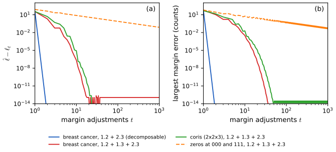
fig_19_s1. Download: PDF · SVGFilling the gap 19.9: closed forms, and one cycle for decomposable models p. 298
For the model \(1.2+2.3\) the MLE is explicit:
\[ \hat m_{ijk}=\frac{n_{ij+}\,n_{+jk}}{n_{+j+}} . \]Proof, and why one cycle suffices
If all margins are positive, this table is positive, and \(\log\hat m=\log n_{ij+}+\log n_{+jk}-\log n_{+j+}\) is a sum of functions of \((x_1,x_2)\), \((x_2,x_3)\) and \(x_2\), so it is in \(V_M\). Its margins: \(\sum_k\hat m_{ijk}=n_{ij+}n_{+j+}/n_{+j+}=n_{ij+}\) and \(\sum_i\hat m_{ijk}=n_{+j+}n_{+jk}/n_{+j+}=n_{+jk}\). By Theorem 19.A(b) it is the MLE.
Iterative proportional fitting from the uniform table \(c\): after the \(1.2\) step, \(m=n_{ij+}/r_3\); after the \(2.3\) step, \(m=(n_{ij+}/r_3)\,n_{+jk}/(n_{+j+}/r_3)=\hat m\). One cycle, exactly.
The same argument gives the other closed forms in the table of Filling the gap 19.6. In general, a model is decomposable when it is graphical and its graph is chordal (every cycle of four or more vertices has a chord). Then the MLE is the product of the clique margins divided by the product of the separator margins, and iterative proportional fitting with the cliques in a suitable order converges in one cycle (Haberman, 1974; Lauritzen, 1996). Among the hierarchical models of three variables, all except \(1.2+1.3+2.3\) behave this way; the code checks the 18 closed forms against the iterative fit. The no-three-way model is the smallest exception: for a \(2\times2\times2\) table its MLE solves a cubic equation (Bartlett, 1935).
19.5.3 Standard errors (added)
p. 298 The book says the Fisher information "is also found numerically". For log-linear models it has a closed form, and the standard errors in Example 19.15 come from it.
Filling the gap 19.10: Fisher information, and why Poisson and multinomial standard errors agree pp. 298–300
Write the fitted counts as \(\log\mu=X\beta\), with \(X\) the corner-point design matrix (one column per parameter, the first for \(\psi_\emptyset\)). Under the Poisson model for the counts (the one R's glm(..., family = poisson) fits), the score is \(X^\T(n-\mu)\) and the Fisher information is
For the saturated model \(X\) is square and invertible and \(\hat\mu=n\), so each \(\hat\beta_A\) is a signed sum of log counts and its standard error is \(\sqrt{\sum1/n(x)}\) over the \(2^{|A|}\) cells involved (binary case): for the intercept \(1/\sqrt{35}=0.169\), for the three-way term \(\sqrt{1/35+1/42+\cdots+1/76}=0.405\), as in the book's first table.
Derivation, and the multinomial version
Information. \(L(\beta)=\sum_x\{n(x)(X\beta)(x)-e^{(X\beta)(x)}\}\) has gradient \(X^\T(n-\mu)\) and Hessian \(-X^\T\operatorname{diag}(\mu)X\), which does not involve \(n\): observed and expected information coincide (the log link is canonical). Newton's method, \(\beta\leftarrow\beta+I(\beta)^{-1}X^\T(n-\mu)\), is therefore also Fisher scoring; the code implements it and reproduces statsmodels' coefficients and standard errors to \(10^{-8}\).
Multinomial. Under the multinomial model the intercept is not a free parameter; with \(Z\) the design without its first column and \(\pi=\mathrm{softmax}(Z\gamma)\), the log-likelihood \(\sum n(x)(Z\gamma)(x)-n\log\sum_xe^{(Z\gamma)(x)}\) has information \(n\{Z^\T\operatorname{diag}(\pi)Z-(Z^\T\pi)(Z^\T\pi)^\T\}\). This is the Schur complement of the intercept block in the Poisson information at \(\hat\mu=n\hat\pi\) (since \(\sum\hat\mu=n\)), and the inverse of a Schur complement is the corresponding block of the inverse. So every non-intercept standard error is the same under both models; only the intercept's differs, and it has no meaning in the multinomial model. The Poisson profile likelihood argument of Filling the gap 19.7 gives the same conclusion for the estimates themselves.
19.5.4 Model selection: AIC and the deviance
pp. 298–299 Which terms should be in the model? One approach is AIC: choose the model that maximises
\[ \AIC(M)=\ell(M)-|M| \tag{19.2} \]where \(\ell(M)\) is the maximised log-likelihood and \(|M|\) the number of parameters (counting \(\psi_\emptyset\), as the book does; only differences matter). The search is usually restricted to hierarchical models. The other approach tests each model against the saturated one.
Definition 19.13 (deviance) p. 299
\(\dev(M)=2(\ell_\sat-\ell_M)\), where \(\ell_\sat\) and \(\ell_M\) are the maximised log-likelihoods of the saturated model and of \(M\). In terms of fitted counts, \(\dev(M)=2\sum_xn(x)\log\{n(x)/\hat m(x)\}\), the likelihood ratio statistic \(G^2\) of Chapter 15.
Theorem 19.14 p. 299
\(\dev(M)\) is the likelihood ratio statistic for \(H_0\): the model is \(M\), against the saturated model. If the true cell probabilities are positive and \(M\) holds, \(\dev(M)\) converges in distribution to \(\chi^2_\nu\) as \(n\to\infty\), with \(\nu=N-|M|\).
Filling the gap 19.11: the deviance theorem, nested tests, and the conventions for AIC and BIC p. 299
Proof of Theorem 19.14, and the nested version
Likelihood ratio. The saturated MLE is \(\hat p=n/n\) (the observed proportions), so \(\ell_\sat=\sum n(x)\log\{n(x)/n\}\), and \(\dev(M)=2(\ell_\sat-\ell_M)\) is \(-2\log\) of the ratio of maximised likelihoods by definition: the statistic \(\lambda\) of Definition 10.21.
Limit. The saturated model is the open simplex, of dimension \(N-1\). By Filling the gap 19.2, a model \(M\) is the image of an open set of \(\R^{|M|-1}\) (its free parameters other than \(\psi_\emptyset\)) under a smooth one-to-one map with full-rank derivative, so it is a smooth submanifold of dimension \(|M|-1\). When the true \(p\) is in \(M\) and positive (an interior point), Wilks' theorem (Theorem 10.22, with the sketch in Filling the gap 10.12) gives \(\chi^2\) with \((N-1)-(|M|-1)=N-|M|\) degrees of freedom. By Filling the gap 19.2, \(\nu=\sum_{A\notin M}\prod_{j\in A}(r_j-1)\): one degree of freedom per free parameter of each omitted term.
Nested models. For \(M_0\subset M_1\), the likelihood ratio statistic for \(M_0\) against \(M_1\) is \(2(\ell_{M_1}-\ell_{M_0})=\dev(M_0)-\dev(M_1)\), and the same argument gives \(\chi^2_{|M_1|-|M_0|}\) under \(M_0\). Pearson's \(X^2=\sum(n-\hat m)^2/\hat m\) has the same limit.
Simulation. Figure 19.S3 draws 4000 tables of size 474 from the fitted model \(1.2+2.3\) of the breast cancer data. The deviance of \(1.2+2.3\) rejects at 5% in 4.70% of them, and the nested statistic against \(1.2+1.3+2.3\) in 4.50% (both within simulation error of 5%), and their histograms follow \(\chi^2_2\) and \(\chi^2_1\).
Conventions. Since \(\ell_M=\ell_\sat-\dev(M)/2\), maximising \((19.2)\) is minimising \(\dev(M)+2|M|\). R reports \(-2\ell^{\mathrm{Pois}}_M+2|M|\), where \(\ell^{\mathrm{Pois}}\) is the Poisson log-likelihood; it differs from \(-2\AIC(M)\) by a constant that is the same for every model (the code confirms this), so the rankings agree. BIC in the book's convention (Chapter 13) is \(\ell(M)-|M|\log(n)/2\).
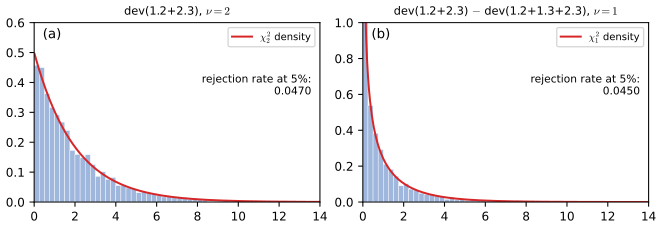
fig_19_s3. Download: PDF · SVGp. 299 The book warns against declaring every model that passes its deviance test "plausible": many tests mean many chances for errors, and a model may pass only because the test has little power.
Filling the gap 19.12: how much power is lost, measured p. 299
Take as truth the no-three-way model fitted to the breast cancer data. Its weakest term is the centre-survival interaction, 0.14 on the log scale (standard error about 0.20 at \(n=474\)). For tables of size \(n\) drawn from it, Figure 19.S4 records which of the nine models each strategy picks (300 tables per \(n\)):
- AIC finds the true model in 15% of tables at \(n=474\), and prefers the simpler \(1.2+2.3\) (49%); the true model wins only for \(n\) in the thousands (71% at \(n=5000\)).
- BIC, with its heavier penalty, picks the true model in 2% of tables at \(n=474\) and 27% at \(n=5000\).
- "The smallest model that passes its deviance test at 5%" picks it in 2% at \(n=474\) and 47% at \(n=5000\).
So with the book's sample size the data cannot distinguish a weak interaction from none, whichever method is used, and the testing strategy is the most conservative. A model chosen this way should be read as "consistent with the data", not as evidence that the omitted terms are zero.
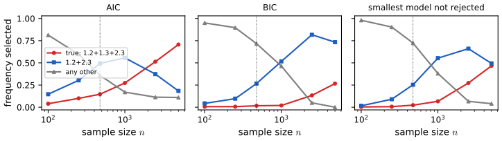
fig_19_s4. Download: PDF · SVGExample 19.15 (breast cancer data). pp. 299–300 Morrison et al. (1973) classified 474 breast cancer patients by diagnostic centre \(X_1\), nuclear grade \(X_2\) and survival \(X_3\):
| malignant, died | malignant, survived | benign, died | benign, survived | |
|---|---|---|---|---|
| Boston | 35 | 59 | 47 | 112 |
| Glamorgan | 42 | 77 | 26 | 76 |
With reference levels Boston, malignant and died, the saturated model (my fit, by Newton's method on the Poisson likelihood; the book prints these values cut to two decimals):
| term | \(\hat\beta\) | \(\widehat{\mathrm{se}}\) | \(W\) | \(p\)-value |
|---|---|---|---|---|
| (intercept) | 3.5553 | 0.1690 | 21.03 | <0.0001 |
| centre | 0.1823 | 0.2289 | 0.80 | 0.426 |
| grade | 0.2948 | 0.2233 | 1.32 | 0.187 |
| survival | 0.5222 | 0.2134 | 2.45 | 0.014 |
| centre×grade | −0.7744 | 0.3348 | −2.31 | 0.021 |
| centre×survival | 0.0839 | 0.2869 | 0.29 | 0.770 |
| grade×survival | 0.3462 | 0.2752 | 1.26 | 0.208 |
| centre×grade×survival | 0.1203 | 0.4051 | 0.30 | 0.766 |
Backward search by AIC removes the three-way term, then the centre-survival term, and stops at \(1.2+2.3\) (Figure 19.S2):
| term | \(\hat\beta\) | \(\widehat{\mathrm{se}}\) | \(W\) | \(p\)-value |
|---|---|---|---|---|
| (intercept) | 3.5258 | 0.1376 | 25.63 | <0.0001 |
| centre | 0.2358 | 0.1380 | 1.71 | 0.087 |
| grade | 0.2690 | 0.1873 | 1.44 | 0.151 |
| survival | 0.5688 | 0.1426 | 3.99 | 6.65e−05 |
| centre×grade | −0.6798 | 0.1874 | −3.63 | 0.0003 |
| grade×survival | 0.3771 | 0.1984 | 1.90 | 0.057 |
Its deviance is \(0.6001\) on \(8-6=2\) degrees of freedom, with \(p=\P(\chi^2_2>0.6001)=e^{-0.30}=0.741\): no evidence of lack of fit. By Filling the gap 19.9 the fitted counts are \(n_{ij+}n_{+jk}/n_{+j+}\) (for example \(94\cdot77/213=33.98\) in the first cell), and the graph is Centre − Grade − Survival (Figure 19.5): centre and survival are independent given grade. The difference in survival between the centres is accounted for by the different mix of grades (63% of Boston's tumours are graded benign, 46% of Glamorgan's), the same conclusion as the edge tests of Exercise 18.5. The search over all 19 hierarchical models (including those without some main effect) selects the same model, and AIC values in the book's convention are \(-946.97\) for \(1.2+2.3\), \(-947.71\) for \(1.2+1.3+2.3\) and \(-948.67\) for the saturated model (R's AIC: 59.20, 60.69, 62.60).
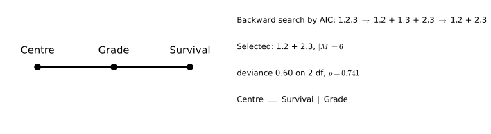
fig_19_5. Download: PDF · SVG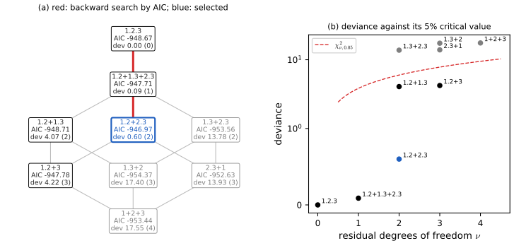
fig_19_s2. Download: PDF · SVG19.6 Bibliographic Remarks
p. 300 The book follows Whittaker (1990); the classic reference is Bishop, Fienberg and Holland (1975). For the results added here: Birch (1963) characterised the MLE by the margins, Deming and Stephan (1940) introduced iterative proportional fitting, Haberman (1974) gave existence conditions and the theory of decomposable models, Csiszár (1975) the information-geometric proof of convergence, and Lauritzen (1996) the graphical-model view of all of these.
Notes on the book
None of the points below is in the author's two errata lists (which have no entries for pages 291–301); each comes with its evidence.
Page 294, proof of Theorem 19.4: "or" should be "and"
The proof says that \(\psi_t\) is 0 if \(t\not\subset a\cup b\) or \(t\not\subset a\cup c\). Taken literally this forces, for example, \(\psi_b=0\) (since \(b\not\subset a\cup c\)), which the hypothesis does not give. The hypothesis says \(\psi_t=0\) when \(t\not\subset a\cup b\) and \(t\not\subset a\cup c\), i.e. when \(t\) meets both \(b\) and \(c\). The displayed decomposition that follows is correct. The converse direction is not a reversal of the argument: it needs the uniqueness of the expansion (Filling the gap 19.3).
Page 292, Theorem 19.1: the probability function must be positive
\(\log f(x)\) is undefined in an empty cell, so the theorem needs \(f(x)>0\) for all \(x\); so does Theorem 19.4 (its "only if" part fails for distributions with zeros, as the three identical coins of Filling the gap 18.4 show for Theorem 18.1). Positivity is also why the MLE can fail to exist with empty cells (Filling the gap 19.8).
Page 294, Definition 19.6: wording
"\(\psi_A(x)=0\) if and only if \(\{i,j\}\subset A\) and \((i,j)\) is not an edge" should read "if and only if \(A\) contains some pair \(\{i,j\}\) that is not an edge"; and "nonzero" should be read as "not constrained to be zero" (a particular distribution in a graphical model may have a free term that happens to vanish). With these readings the definition is Filling the gap 19.4.
Page 300, Example 19.15: the printed values are cut, not rounded
Except for the intercept row of the first table, every entry of the two tables is my value truncated to two decimals: for example the standard error 0.2869 of centre×survival is printed 0.28, the Wald statistic 2.4475 of survival 2.44, and the \(p\)-value 0.4257 of centre 0.42. The code confirms that truncation reproduces all 28 entries of rows 2 to 8 of the first table, and that every entry of both tables is within 0.01 of the fit. The numbers are therefore correct; differences of one in the last digit from other software are display, not computation.
Page 301, Exercise 19.6: the constants cannot be log-probabilities
Each model is written with \(\log f=7+\cdots\), but then \(f(0,0,0,0)=e^7>1\). The intercepts must be read as "up to the normalising constant" (\(\psi_\emptyset\) is fixed by the other terms, Filling the gap 19.2). The question asked, graphical or hierarchical, depends only on which terms are present, so the answers are unaffected.
Page 298: "the MLE generally has to be found numerically"
True for some models, but most small models have closed forms, including the model selected in Example 19.15 (Filling the gap 19.9); and the Fisher information is explicit, \(X^\T\operatorname{diag}(\hat\mu)X\) (Filling the gap 19.10). Also, in Example 19.3 the six parameters are not free: one is fixed by normalisation, which is why \(\Theta\) has dimension \(N-1=5\).
19.7 Exercises
All six exercises of Chapter 19 (Wasserman, 2004, pp. 300–301), restated in my own words, with complete solutions (hidden).
Exercise 19.1. In Example 19.3, express the cell probabilities \(p_{ij}\) in terms of \(\beta_1,\dots,\beta_6\).
Solution
Evaluate \((19.1)\) at each cell; only the terms whose indicators are 1 contribute:
\[ p_{00}=e^{\beta_1},\quad p_{10}=e^{\beta_1+\beta_2},\quad p_{01}=e^{\beta_1+\beta_3},\quad p_{02}=e^{\beta_1+\beta_4}, \] \[ p_{11}=e^{\beta_1+\beta_2+\beta_3+\beta_5},\qquad p_{12}=e^{\beta_1+\beta_2+\beta_4+\beta_6}. \]Since the six probabilities sum to 1, \(\beta_1\) is determined by the others:
\[ \beta_1=-\log\big(1+e^{\beta_2}+e^{\beta_3}+e^{\beta_4}+e^{\beta_2+\beta_3+\beta_5}+e^{\beta_2+\beta_4+\beta_6}\big). \]Substituting \(\beta_5=\log\{p_{11}p_{00}/(p_{01}p_{10})\}\) back confirms \(p_{11}\); the code checks the round trip on a random table.
Exercise 19.2. Prove Lemma 19.5.
Solution
See Filling the gap 19.3 (first proof): if \(X_b\indep X_c\given X_a\), take \(g=f(x_a,x_b)\) and \(h=f(x_c\given x_a)\) (0 where \(f(x_a)=0\)); conversely, summing \(f=gh\) over \(x_b\), \(x_c\) or both shows \(f(x_b,x_c\given x_a)=f(x_b\given x_a)f(x_c\given x_a)\) wherever \(f(x_a)>0\).
Exercise 19.3. Prove Lemma 19.9.
Solution
See Filling the gap 19.5: the terms of a graphical model are the complete sets of its graph, and subsets of complete sets are complete, so the model is hierarchical. The no-three-way model \(1.2+1.3+2.3\) (Example 19.11) is hierarchical but not graphical.
Exercise 19.4. For \((X_1,X_2,X_3,X_4)\) with \(\log f=\psi_\emptyset+\psi_{12}+\psi_{13}+\psi_{24}+\psi_{34}\): (a) draw the graph; (b) list the independence and conditional independence relations it implies; (c) is the model graphical, hierarchical?
Solution
(a) Edges 1-2, 1-3, 2-4, 3-4: the four-cycle \(X_1-X_2-X_4-X_3-X_1\) (no diagonals 1-4 or 2-3).
(b) Pairwise, by Theorem 19.4: \(X_1\indep X_4\given(X_2,X_3)\) and \(X_2\indep X_3\given(X_1,X_4)\). These are also the only separation statements: opposite corners of a cycle are separated only by the two other vertices, and no marginal independence holds (the graph is connected). For a positive \(f\) in the model the global Markov property adds nothing new (Exercise 18.3(c) lists the same minimal statements for the four-cycle). The code confirms both statements on a random member of the model (conditional mutual information 0 to \(10^{-13}\)).
(c) Neither. \(\psi_{12}\) is present while \(\psi_1\) and \(\psi_2\) are not, so the model is not hierarchical, and hence not graphical (Lemma 19.9). Its hierarchical closure \(1.2+1.3+2.4+3.4\) is graphical: the cliques of a four-cycle are its vertices and edges. The model as written is the closure with all four main effects forced to 0, constraints that depend on the coding of the levels (Filling the gap 19.5). Try it in the graphical versus hierarchical demo.
Exercise 19.5. Binary \(X_1,X_2,X_3\) have \(p(x_1,x_2,x_3)\) proportional to the values below. Find the \(\psi\)-terms and comment.
\(x_2=0,x_3=0\) \(x_2=0,x_3=1\) \(x_2=1,x_3=0\) \(x_2=1,x_3=1\) \(x_1=0\) 2 8 4 16 \(x_1=1\) 16 128 32 256 Solution
The values sum to 462. With the Möbius formula (binary case: \(\psi_A(x)=\beta_A\prod_{j\in A}x_j\)):
\[ \beta_\emptyset=\log\tfrac{2}{462},\quad \beta_1=\log\tfrac{16}{2}=\log8,\quad \beta_2=\log\tfrac42=\log2,\quad \beta_3=\log\tfrac82=\log4, \] \[ \beta_{12}=\log\tfrac{32\cdot2}{16\cdot4}=0,\quad \beta_{13}=\log\tfrac{128\cdot2}{16\cdot8}=\log2,\quad \beta_{23}=\log\tfrac{16\cdot2}{4\cdot8}=0, \] \[ \beta_{123}=\log\tfrac{256\cdot16\cdot4\cdot8}{32\cdot128\cdot16\cdot2}=0 . \]So \(\log p=\log\tfrac2{462}+x_1\log8+x_2\log2+x_3\log4+x_1x_3\log2\): the model \(1.3+2\). By Theorem 19.4, \(X_2\indep(X_1,X_3)\), with \(\P(X_2=1)=2/3\) (every entry doubles when \(x_2\) goes from 0 to 1), while \(X_1\) and \(X_3\) are associated with odds ratio 2. The model is graphical (graph: the single edge 1-3 and the isolated vertex 2) and hierarchical. The code reproduces all eight terms to \(10^{-12}\).
Exercise 19.6. For binary \(X_1,\dots,X_4\), draw the graph of each model and say whether it is graphical and/or hierarchical: (a) \(\log f=7+11x_1+2x_2+1.5x_3+17x_4\); (b) the main effects of (a) plus \(12x_2x_3+78x_2x_4+3x_3x_4+32x_2x_3x_4\); (c) the main effects plus \(12x_2x_3+3x_3x_4+x_1x_4+2x_1x_2\); (d) \(\log f=7+5055x_1x_2x_3x_4\).
Solution
For binary variables each term is \(\beta_A\prod_{j\in A}x_j\), so a monomial with a nonzero coefficient is a present term. (The constants such as 7 cannot be \(\psi_\emptyset\), see the notes on the book; read them up to normalisation.)
(a) Main effects only: no edges, mutual independence. Its terms (\(\emptyset\) and singletons) are exactly the complete sets of the empty graph: graphical and hierarchical.
(b) Terms 23, 24, 34, 234 with all main effects: the triangle on \(\{2,3,4\}\) and the isolated vertex 1. Complete sets: \(\emptyset\), the singletons, 23, 24, 34, 234; all present: graphical (generator \(2.3.4+1\)), hence hierarchical. \(X_1\indep(X_2,X_3,X_4)\).
(c) Terms 12, 14, 23, 34: the four-cycle \(1-2-3-4-1\). Its complete sets are the vertices and the four edges (no triangles), all present: graphical (generator \(1.2+2.3+3.4+1.4\)) and hierarchical. \(X_1\indep X_3\given(X_2,X_4)\), \(X_2\indep X_4\given(X_1,X_3)\).
(d) Only \(\psi_{1234}\): the graph is complete, but the main effects and lower interactions are missing, so the model is not hierarchical and not graphical. The code and the graphical versus hierarchical demo give the same four answers.
Demonstrations for this chapter
Each demonstration runs in the browser and links back to these notes. The ▶ Demo boxes above open them already set to the case under discussion.
| Demonstration | What you can see | Sections and results |
|---|---|---|
| Iterative proportional fitting | Any of the nine hierarchical models fitted to the breast cancer table, the \(2\times2\times3\) coris table or a table with two zeros, one margin adjustment at a time: observed and fitted counts, the log-likelihood gap and the margin errors, the generator margins, and the three-way log odds ratio that the algorithm never changes. Presets: 1 the selected model of Example 19.15 in one cycle; 2 no three-way interaction; 3 the coris table; 4 a start outside the model; 5 an MLE that does not exist. | 19.5.2; Theorems 19.A, 19.B; Filling the gaps 19.8, 19.9 |
| Graphical versus hierarchical models | Toggle the terms of a model on 3, 4 or 5 variables; see its graph, the lattice of all terms coloured by status, whether it is hierarchical and graphical, its generator, and the independences it implies. Presets: 1 Example 19.7; 2 Example 19.7 without three-way terms; 3 Example 19.11; 4 Example 19.12; 5 Exercise 19.4. | 19.2–19.4; Theorem 19.4, Lemma 19.9; Filling the gaps 19.4, 19.5 |
| Model selection across the hierarchy | All nine hierarchical models of a three-way table on the lattice, with deviance, AIC, BIC and the backward search, for the book's data, the coris table or tables simulated from a chosen model and sample size. Presets: 1 Example 19.15 by AIC; 2 by deviance tests; 3 the coris table; 4 a weak interaction at \(n=474\); 5 at \(n=5000\). | 19.5.4; Theorem 19.14; Filling the gaps 19.11, 19.12; Example 19.15 |
Related demonstrations: in this course, the cliques and potentials demo of Chapter 18 (interaction terms vanish off the cliques) and the model selection scores demo of Chapter 13; in the companion course Statistical Learning: Theory and Methods, the graphical lasso demo. The Python code that produces every figure of this page is code/ch19_log_linear_models.py (see the code index).
References
- Wasserman, L. (2004). All of Statistics: A Concise Course in Statistical Inference. Springer, New York. Chapter 19, pp. 291–301. www.stat.cmu.edu/~larry/all-of-statistics.
- Bartlett, M. S. (1935). Contingency table interactions. Supplement to the Journal of the Royal Statistical Society, 2(2), 248–252.
- Birch, M. W. (1963). Maximum likelihood in three-way contingency tables. Journal of the Royal Statistical Society, Series B, 25(1), 220–233.
- Bishop, Y. M. M., Fienberg, S. E. and Holland, P. W. (1975). Discrete Multivariate Analysis: Theory and Practice. MIT Press, Cambridge, MA.
- Csiszár, I. (1975). I-divergence geometry of probability distributions and minimization problems. The Annals of Probability, 3(1), 146–158.
- Deming, W. E. and Stephan, F. F. (1940). On a least squares adjustment of a sampled frequency table when the expected marginal totals are known. The Annals of Mathematical Statistics, 11(4), 427–444.
- Fienberg, S. E. (1970). An iterative procedure for estimation in contingency tables. The Annals of Mathematical Statistics, 41(3), 907–917.
- Haberman, S. J. (1974). The Analysis of Frequency Data. University of Chicago Press, Chicago.
- Lauritzen, S. L. (1996). Graphical Models. Oxford University Press, Oxford.
- Morrison, A. S., Black, M. M., Lowe, C. R., MacMahon, B. and Yuasa, S. (1973). Some international differences in histology and survival in breast cancer. International Journal of Cancer, 11(2), 261–267.
- Whittaker, J. (1990). Graphical Models in Applied Multivariate Statistics. Wiley, Chichester.
The numerical statements in the text (the expansions and parameter counts, the independence criteria, the classification of every example and exercise, the model counts, the fits and tables of Example 19.15, Birch's margin equations, the monotonicity and limits of iterative proportional fitting, the closed forms, the standard errors under both sampling models, the null distributions of the deviance and the selection frequencies) were confirmed numerically.