Sequential Data
When observations arrive in order (speech frames, sensor readings, characters, nucleotides), neighbouring values are related and the independence assumption of the earlier chapters fails. This chapter builds models for such data from a hidden Markov chain: discrete hidden states give the hidden Markov model, Gaussian hidden states give the linear dynamical system. For both, inference along the chain costs time linear in its length, through forward and backward recursions (forward-backward and Viterbi; the Kalman filter and the Rauch-Tung-Striebel smoother), and the parameters are learned by EM. When the model is neither discrete nor linear-Gaussian, particle filters take over. Every step the book leaves to the reader is written out below.
Ch. 1 Introduction Ch. 2 Probability distributions Ch. 3 Linear regression Ch. 4 Linear classification Ch. 5 Neural networks Ch. 6 Kernel methods Ch. 7 Sparse kernel machines Ch. 8 Graphical models Ch. 9 Mixture models and EM Ch. 10 Approximate inference Ch. 11 Sampling methods Ch. 12 Continuous latent variables Ch. 13 Sequential data Ch. 14 Combining models
How to read these notes
They follow the book. Sections carry Bishop's numbers (13.1, 13.2.2, ...) and every displayed equation that appears in the book carries the book's own equation number, e.g. (13.36), so you can read these notes next to the book. Equations without a number are steps that the book skips.
Filling the gaps. Wherever the book says that a result "is easily verified", follows "after some manipulation", or is left as an exercise, an orange Filling the gap box or a proof gives the full argument. Proofs and derivations start hidden: open one with its bar, or use the button below.
Figures and demonstrations. The numerical figures of the chapter are reproduced from scratch by the Python code; the graphical models are redrawn. The ▶ Demo boxes open an interactive demonstration already set to the case being discussed. Gaussian identities (completing the square, the linear-Gaussian model, the Woodbury identity) are proved once in the mathematical toolkit.
Main reference
C. M. Bishop, Pattern Recognition and Machine Learning, Springer (2006), Chapter 13, pages 605–652. Section, equation, figure and exercise numbers below refer to this book. Further reading is listed in the references.
The explanations, derivations and code are my own; equations are cited by their numbers in the book.
The chapter at a glance
- 13.1 Markov chains of order \(M\) make the next observation depend on the last \(M\) only; a discrete chain needs \(K^M(K-1)\) parameters, which explodes with \(M\). Putting the Markov chain on latent variables (the state space model, Figure 13.5) keeps the parameter count fixed but makes the observations depend on the whole past (Result 13.4).
- 13.2 The hidden Markov model: a discrete hidden chain with transition matrix \(\mathbf{A}\) and an emission density per state. EM (Baum-Welch) needs only the single and pairwise posteriors \(\gamma(\mathbf{z}_n)\), \(\xi(\mathbf{z}_{n-1},\mathbf{z}_n)\), which the forward-backward recursions deliver in \(O(K^2N)\) operations instead of \(K^N\). Rescaling keeps the numbers in range and gives the log likelihood as \(\sum_n\ln c_n\). The Viterbi algorithm finds the single most probable state sequence, which is not the sequence of individually most probable states.
- 13.3 The linear dynamical system: Gaussian hidden states with linear dynamics and linear-Gaussian emissions. The forward recursion is the Kalman filter (predict, then correct with a gain), the backward one the Rauch-Tung-Striebel smoother, and EM has closed-form M steps. Non-linear or non-Gaussian models are handled approximately: the extended Kalman filter linearises, the particle filter uses sequential importance resampling.
Notation. Observations \(\mathbf{X}=\{\mathbf{x}_1,\dots,\mathbf{x}_N\}\), latent variables \(\mathbf{Z}=\{\mathbf{z}_1,\dots,\mathbf{z}_N\}\). For the HMM, \(\mathbf{z}_n\) is a 1-of-\(K\) binary vector and \(z_{nk}=1\) means "state \(k\) at time \(n\)"; \(\sum_{\mathbf{z}_n}\) sums over its \(K\) values. Short-hand for runs: \(\mathbf{x}_{1:n}\)
Prerequisites. Directed graphs, d-separation and the sum-product and max-sum algorithms (Chapter 8, especially Section 8.2 and 8.4.4–8.4.5), the EM algorithm (Sections 9.3 and 9.4), Gaussian conditionals and marginals (toolkit), Lagrange multipliers (toolkit), and importance resampling (Section 11.1.5).
Printings. The text used here is a corrected printing. Where Bishop's errata list corrects an equation of this chapter, the notes give the corrected form and a short Erratum note naming the original.
Sequences and state space models
pp. 605–607 So far the data points were independent and identically distributed, so the likelihood was a product over points. Many data sets are ordered instead: rainfall on successive days, exchange rates, the acoustic spectrum of speech in successive time frames (Figure 13.1), but also positions along a DNA strand or a sentence. Words such as "past" and "future" are used for convenience; nothing below needs the index to be time.
Two distinctions organise the chapter. A sequence is stationary if the mechanism generating it does not change along the sequence (the data change, the distribution does not); the chapter treats only this case. And a model must let recent observations matter more than old ones without letting the number of parameters grow with the length of the sequence. Markov models (Section 13.1) do this by forgetting everything but the last few observations; state space models do it by routing all dependence through a hidden Markov chain.
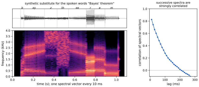
fig13_1. Download: PDF · SVG13.1 Markov models
pp. 607–610 Ignoring the order and treating the observations as i.i.d. (Figure 13.2, a graph with no edges) throws away exactly what makes sequences predictable: whether it rained today says a lot about tomorrow, but under an i.i.d. model the only usable information is the overall frequency of rainy days. Without any assumption, the product rule always gives
\[ p(\mathbf{x}_1,\dots,\mathbf{x}_N)=p(\mathbf{x}_1)\prod_{n=2}^{N}p(\mathbf{x}_n\given\mathbf{x}_1,\dots,\mathbf{x}_{n-1}). \tag{13.1} \]Erratum. The book's (13.1) omits the factor \(p(\mathbf{x}_1)\); the form above is the corrected one.
Definition 13.1 (Markov chain of order \(M\); homogeneous chain) pp. 607–609, (13.2), (13.4)
A sequence is a first-order Markov chain if its joint distribution has the form
\[ p(\mathbf{x}_1,\dots,\mathbf{x}_N)=p(\mathbf{x}_1)\prod_{n=2}^{N}p(\mathbf{x}_n\given\mathbf{x}_{n-1}), \tag{13.2} \]the directed graph of Figure 13.3. It is a second-order Markov chain if
\[ p(\mathbf{x}_1,\dots,\mathbf{x}_N)=p(\mathbf{x}_1)\,p(\mathbf{x}_2\given\mathbf{x}_1)\prod_{n=3}^{N}p(\mathbf{x}_n\given\mathbf{x}_{n-1},\mathbf{x}_{n-2}), \tag{13.4} \](Figure 13.4), and of order \(M\) if each factor conditions on the previous \(M\) values (on all previous ones while \(n\le M\)). The chain is homogeneous if the conditional distributions \(p(\mathbf{x}_n\given\cdot)\) are the same function for every \(n\), so that they share their parameters.
The point of (13.2) is that, once the previous value is known, the rest of the past is irrelevant for predicting the next value. The book says this follows from d-separation or is "easily verified by direct evaluation" (p. 608, Exercises 13.1 and 13.2). Here are both arguments, for orders one and two.
Result 13.1 (the first-order Markov property; Exercises 13.1 and 13.2) p. 608, (13.3)
If the joint distribution has the form (13.2), then for \(n=2,\dots,N\)
\[ p(\mathbf{x}_n\given\mathbf{x}_1,\dots,\mathbf{x}_{n-1})=p(\mathbf{x}_n\given\mathbf{x}_{n-1}). \tag{13.3} \]More generally, given \(\mathbf{x}_n\), the past \(\mathbf{x}_{1:n-1}\) and the future \(\mathbf{x}_{n+1:N}\) are independent.
Proof (by the sum and product rules, and by d-separation)
Marginals of a chain are chains. Summing (13.2) over \(\mathbf{x}_N\) removes the last factor, because \(\sum_{\mathbf{x}_N}p(\mathbf{x}_N\given\mathbf{x}_{N-1})\)
(Sum the innermost variable \(\mathbf{x}_N\) first, then \(\mathbf{x}_{N-1}\), and so on: at each stage the variable being summed appears in exactly one remaining factor, which sums to one.)
The Markov property. By the definition of a conditional distribution and the display above with \(n\) and \(n-1\),
\[ p(\mathbf{x}_n\given\mathbf{x}_{1:n-1})=\frac{p(\mathbf{x}_{1:n})}{p(\mathbf{x}_{1:n-1})}=\frac{p(\mathbf{x}_1)\prod_{m=2}^{n}p(\mathbf{x}_m\given\mathbf{x}_{m-1})}{p(\mathbf{x}_1)\prod_{m=2}^{n-1}p(\mathbf{x}_m\given\mathbf{x}_{m-1})}=p(\mathbf{x}_n\given\mathbf{x}_{n-1}). \]The factor \(p(\mathbf{x}_n\given\mathbf{x}_{n-1})\) appearing here is the model's conditional, and it is also the conditional of the joint: summing \(p(\mathbf{x}_{n-1},\mathbf{x}_n)\)
Past and future given the present. \(p(\mathbf{x}_{1:N})\) factorises as \(\big[p(\mathbf{x}_1)\prod_{m\le n}p(\mathbf{x}_m\given\mathbf{x}_{m-1})\big]\)
By d-separation (Section 8.2). In Figure 13.3a every path from \(\mathbf{x}_m\), \(m\lt n-1\), to \(\mathbf{x}_n\) runs along the chain and passes through \(\mathbf{x}_{n-1}\), where the arrows meet head-to-tail. The node \(\mathbf{x}_{n-1}\) is in the conditioning set, so every such path is blocked and \(\mathbf{x}_n\perp\!\!\!\perp\mathbf{x}_{1:n-2}\given\mathbf{x}_{n-1}\), which is (13.3). ∎
Result 13.2 (the second-order Markov property; Exercises 13.1 and 13.2) p. 608, (13.122)–(13.123)
If the joint distribution has the form (13.4), then for \(n=3,\dots,N\)
\[ p(\mathbf{x}_n\given\mathbf{x}_1,\dots,\mathbf{x}_{n-1})=p(\mathbf{x}_n\given\mathbf{x}_{n-1},\mathbf{x}_{n-2}). \tag{13.122} \]The same argument gives \(p(\mathbf{x}_n\given\mathbf{x}_{1:n-1})\)
Proof
Sum and product rules. Exactly as before, summing (13.4) over \(\mathbf{x}_N\), then \(\mathbf{x}_{N-1}\), and so on down to \(\mathbf{x}_{n+1}\), removes one normalised factor at a time (each \(\mathbf{x}_m\) with \(m\gt n\) appears, when it is summed, only in its own factor \(p(\mathbf{x}_m\given\mathbf{x}_{m-1},\mathbf{x}_{m-2})\), because the factors of later variables have already been removed). Hence \(p(\mathbf{x}_{1:n})\)
By d-separation. In Figure 13.3b, take any path from \(\mathbf{x}_m\), \(m\le n-3\), to \(\mathbf{x}_n\), with conditioning set \(\{\mathbf{x}_{n-1},\mathbf{x}_{n-2}\}\). All edges point forward in time. Case 1: the path enters \(\mathbf{x}_n\) from a parent \(\mathbf{v}\in\{\mathbf{x}_{n-1},\mathbf{x}_{n-2}\}\). The edge \(\mathbf{v}\to\mathbf{x}_n\) leaves \(\mathbf{v}\), so the path is head-to-tail or tail-to-tail at \(\mathbf{v}\) (and \(\mathbf{v}\ne\mathbf{x}_m\) since \(m\le n-3\)); \(\mathbf{v}\) is observed, so the path is blocked. Case 2: the path enters \(\mathbf{x}_n\) from a child. Then it visits a node later than \(\mathbf{x}_n\); let \(\mathbf{x}_t\), \(t\gt n\), be the latest node on the path. Both its neighbours on the path are earlier, and edges point forward in time, so both edges point into \(\mathbf{x}_t\): the path is head-to-head there. Every descendant of \(\mathbf{x}_t\) is later than \(n\), hence unobserved, so the path is blocked at \(\mathbf{x}_t\). Either way \(\mathbf{x}_n\perp\!\!\!\perp\mathbf{x}_{1:n-3}\given\mathbf{x}_{n-1},\mathbf{x}_{n-2}\). (This is the directed local Markov property: a node is independent of its non-descendants given its parents.) ∎
Result 13.3 (how many parameters) p. 609
For discrete \(\mathbf{x}_n\) with \(K\) states and general conditional probability tables, a homogeneous chain of order \(M\) has \(K^M(K-1)\) free parameters in its transition tables (plus \(K^M-1\) for the first \(M\) values). For a homogeneous order-\(M\) autoregressive model of a \(D\)-dimensional continuous \(\mathbf{x}\), \(p(\mathbf{x}_n\given\mathbf{x}_{n-M:n-1})\)
Proof
An order-\(M\) table assigns a distribution over the \(K\) values of \(\mathbf{x}_n\) to each of the \(K^M\) configurations of \((\mathbf{x}_{n-M},\dots,\mathbf{x}_{n-1})\). A distribution over \(K\) values has \(K-1\) free numbers (they sum to one), so the table has \(K^M(K-1)\). For \(M=1\) this is \(K(K-1)\), the count in the book. In the Gaussian case each \(\mathbf{W}_m\) is \(D\times D\), \(\mathbf{b}\) has \(D\) entries and the symmetric \(\bm\Sigma\) has \(D(D+1)/2\). Tables grow exponentially with \(M\) because they allow any interaction between the \(M\) conditioning values; the autoregressive model allows only additive (linear) effects, which is why it grows linearly. ∎
Erratum. Some printings give the count as \(K^{M-1}(K-1)\) on p. 609; the correct count is \(K^M(K-1)\).
A neural network that takes the last \(M\) values as inputs (the "tapped delay line" of p. 609) is a third option, with a parameter count set by the network rather than by \(K^M\).
State space models
pp. 609–610 To get dependence on the whole past from a fixed, small number of parameters, give each observation a latent variable \(\mathbf{z}_n\) (of any type and dimension) and let the latent variables, not the observations, form a first-order Markov chain:
\[ \mathbf{z}_{n+1}\perp\!\!\!\perp\mathbf{z}_{n-1}\given\mathbf{z}_n , \tag{13.5} \] \[ p(\mathbf{x}_1,\dots,\mathbf{x}_N,\mathbf{z}_1,\dots,\mathbf{z}_N)=p(\mathbf{z}_1)\left[\prod_{n=2}^{N}p(\mathbf{z}_n\given\mathbf{z}_{n-1})\right]\prod_{n=1}^{N}p(\mathbf{x}_n\given\mathbf{z}_n). \tag{13.6} \]This is the state space model of Figure 13.5. With discrete \(\mathbf{z}_n\) it is the hidden Markov model (Section 13.2); with linear-Gaussian conditionals throughout it is the linear dynamical system (Section 13.3).
Result 13.4 (latent chains give dependence of unbounded order; Exercise 13.3) p. 610
(a) In the graph of Figure 13.5, no two observations \(\mathbf{x}_m,\mathbf{x}_n\) are d-separated by any set of other observations. Hence the graph implies no conditional independence among the \(\mathbf{x}\)'s, and in particular no Markov property of any finite order.
(b) This is not only a statement about the graph: there are HMMs in which \(p(\mathbf{x}_{n+1}\given\mathbf{x}_{1:n})\) depends on every one of \(\mathbf{x}_1,\dots,\mathbf{x}_n\), for every \(n\). Example: two hidden states that never switch (\(\mathbf{A}=\mathbf{I}\), \(\pi_1=\pi_2=\frac12\)) and binary emissions with \(p(x=1\given\text{state }1)=0.8\), \(p(x=1\given\text{state }2)=0.2\). If \(k\) of the first \(n\) observations equal 1,
\[ p(x_{n+1}=1\given x_{1:n})=\frac{0.8\cdot4^{2k-n}+0.2}{4^{2k-n}+1}, \]which changes whenever any single \(x_m\), \(m\le n\), is flipped.
(c) The number of parameters does not grow with the order of dependence: an HMM has \(K-1\) initial, \(K(K-1)\) transition and \(K\) sets of emission parameters, whatever \(N\).
Proof
(a) Take \(m\lt n\) and any conditioning set \(\mathcal{C}\) of observed nodes not containing \(\mathbf{x}_m,\mathbf{x}_n\). The path \(\mathbf{x}_m\leftarrow\mathbf{z}_m\)
(b) With \(\mathbf{A}=\mathbf{I}\) the hidden state is drawn once and kept, so given the state the \(x_m\) are i.i.d. Bernoulli. By Bayes' theorem the posterior odds of state 1 after \(k\) ones in \(n\) trials are
\[ \frac{p(\text{state }1\given x_{1:n})}{p(\text{state }2\given x_{1:n})}=\frac{\tfrac12\,0.8^k\,0.2^{n-k}}{\tfrac12\,0.2^k\,0.8^{n-k}}=4^{k}\,4^{-(n-k)}=4^{2k-n}=:r . \]So \(p(\text{state }1\given x_{1:n})=r/(1+r)\), and \(p(x_{n+1}=1\given x_{1:n})\)
(c) Count the free numbers in \(\bm\pi\), \(\mathbf{A}\) and the emission parameters \(\bm\phi_1,\dots,\bm\phi_K\) of Section 13.2; none of them is indexed by \(n\). ∎
13.2 Hidden Markov models
pp. 610–615 A hidden Markov model (HMM) is the state space model (13.6) with a discrete latent variable. Looking at a single time step, \(p(\mathbf{x}_n)\)
Definition 13.2 (hidden Markov model) pp. 610–612, (13.7)–(13.10)
Let \(\mathbf{z}_n\in\{0,1\}^K\) with \(\sum_kz_{nk}=1\) (1-of-\(K\) coding). The transition probabilities \(A_{jk}=p(z_{nk}=1\given z_{n-1,j}=1)\) satisfy \(0\le A_{jk}\le1\), \(\sum_kA_{jk}=1\) (each row of \(\mathbf{A}\) is a distribution, so \(\mathbf{A}\) has \(K(K-1)\) free parameters), the initial probabilities are \(\pi_k=p(z_{1k}=1)\) with \(\sum_k\pi_k=1\), and the emission densities are \(p(\mathbf{x}\given\bm\phi_k)\), one per state. In the 1-of-\(K\) notation,
\[ p(\mathbf{z}_n\given\mathbf{z}_{n-1},\mathbf{A})=\prod_{k=1}^{K}\prod_{j=1}^{K}A_{jk}^{\,z_{n-1,j}z_{nk}}, \tag{13.7} \] \[ p(\mathbf{z}_1\given\bm\pi)=\prod_{k=1}^{K}\pi_k^{\,z_{1k}}, \tag{13.8} \] \[ p(\mathbf{x}_n\given\mathbf{z}_n,\bm\phi)=\prod_{k=1}^{K}p(\mathbf{x}_n\given\bm\phi_k)^{z_{nk}}, \tag{13.9} \]and the joint distribution of a homogeneous HMM, with \(\bm\theta=\{\bm\pi,\mathbf{A},\bm\phi\}\), is
\[ p(\mathbf{X},\mathbf{Z}\given\bm\theta)=p(\mathbf{z}_1\given\bm\pi)\left[\prod_{n=2}^{N}p(\mathbf{z}_n\given\mathbf{z}_{n-1},\mathbf{A})\right]\prod_{m=1}^{N}p(\mathbf{x}_m\given\mathbf{z}_m,\bm\phi). \tag{13.10} \]Why the products (13.7)–(13.9) are right: if \(z_{n-1,j}=1\) and \(z_{nk}=1\), every exponent \(z_{n-1,j'}z_{nk'}\) is zero except the one with \((j',k')=(j,k)\), so the double product is the single number \(A_{jk}\); likewise (13.8) picks out \(\pi_k\) and (13.9) picks out \(p(\mathbf{x}_n\given\bm\phi_k)\). Writing the model this way makes the logarithm linear in the \(z\)'s, which is what makes the E step of Section 13.2.1 need only the marginals of single \(\mathbf{z}_n\) and pairs \((\mathbf{z}_{n-1},\mathbf{z}_n)\). Two pictures of \(\mathbf{A}\) are useful: the state transition diagram (Figure 13.6, nodes are states of one variable, not variables, hence boxes) and its unfolding in time, the lattice or trellis (Figure 13.7). A mixture model for i.i.d. data is the special case where all rows of \(\mathbf{A}\) are equal, so \(p(\mathbf{z}_n\given\mathbf{z}_{n-1})\) does not depend on \(\mathbf{z}_{n-1}\): the horizontal links of Figure 13.5 disappear. The emission densities can be Gaussians, mixtures of Gaussians, tables for discrete \(\mathbf{x}\), or even discriminative models such as neural networks (Exercise 13.4); the inference algorithms below never look inside them, they only use the \(N\times K\) numbers \(p(\mathbf{x}_n\given\bm\phi_k)\).
Sampling, and the stationary behaviour of the hidden chain
pp. 612–613 The joint (13.10) is a directed graph, so it can be sampled by ancestral sampling (Section 8.1.2; see the introduction to Chapter 11): draw \(\mathbf{z}_1\) from \(\bm\pi\), then \(\mathbf{x}_1\) from \(p(\mathbf{x}\given\bm\phi_{k})\) for the drawn state \(k\), then \(\mathbf{z}_2\) from row \(k\) of \(\mathbf{A}\), and so on. When the diagonal of \(\mathbf{A}\) dominates, the sample has long runs from one component (Figure 13.8).
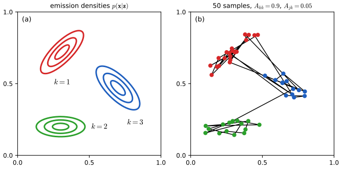
fig13_8. Download: PDF · SVGThe book restricts attention to homogeneous models, where \(\mathbf{A}\) and \(\bm\phi\) do not depend on \(n\). Homogeneous does not yet mean stationary in the sense of the introduction: the distribution of \(\mathbf{z}_n\) still changes with \(n\) unless it starts in the right place. The next result makes this precise.
Result 13.5 (stationary distribution of the hidden chain)
Write distributions over the \(K\) states as row vectors. (a) If \(\mathbf{z}_n\) has distribution \(\mathbf{p}_n\), then \(\mathbf{p}_{n+1}=\mathbf{p}_n\mathbf{A}\), so \(\mathbf{p}_n=\bm\pi^\T\mathbf{A}^{n-1}\). (b) Every stochastic matrix \(\mathbf{A}\) has at least one stationary distribution \(\bm\pi^\star\), i.e. \(\bm\pi^{\star\T}\mathbf{A}=\bm\pi^{\star\T}\). (c) If \(\bm\pi=\bm\pi^\star\), then every \(\mathbf{z}_n\) has distribution \(\bm\pi^\star\), and the whole HMM is strictly stationary: for every \(s\ge0\), the joint distribution of \((\mathbf{z}_{n},\mathbf{x}_n,\dots,\mathbf{z}_{n+s},\mathbf{x}_{n+s})\) is the same for all \(n\). (d) If some power \(\mathbf{A}^m\) has all entries positive, \(\bm\pi^\star\) is unique and \(\mathbf{p}_n\to\bm\pi^\star\) geometrically fast from any \(\bm\pi\), so a homogeneous HMM becomes stationary after a burn-in.
Proof
(a) By the sum rule, \(p(z_{n+1,k}=1)\)
(b) The set \(\Delta\) of probability vectors is closed and bounded, and \(\mathbf{p}\mapsto\mathbf{p}\mathbf{A}\) maps it into itself (entries stay nonnegative and \(\mathbf{p}\mathbf{A}\mathbf{1}\)
(c) By (a), \(\mathbf{p}_n\)
With homogeneous factors and \(\mathbf{p}_n=\bm\pi^{\star\T}\), the right-hand side does not depend on \(n\).
(d) This is the convergence theorem for finite Markov chains, proved in Result 11.17 (with \(T=\mathbf{A}\)). ∎
In practice \(\bm\pi\) is a free parameter, estimated by EM like the others, so a fitted HMM need not start in its stationary distribution; with a single long training sequence \(\bm\pi\) is poorly determined anyway (it is informed by one state, \(\mathbf{z}_1\)).
Left-to-right models
pp. 613–615 Constraints on \(\mathbf{A}\) give useful variants (Rabiner, 1989). In a left-to-right HMM \(A_{jk}=0\) for \(k\lt j\): the state index never decreases, so a state once left can never be re-entered (Figure 13.9). Usually every sequence starts in state 1 (\(\pi_1=1\)), and jumps are limited to \(\Delta\) states, \(A_{jk}=0\) for \(k\gt j+\Delta\) (Figure 13.10 shows \(\Delta=1\)). Then \(\mathbf{A}\) is upper triangular (banded), the last state is absorbing (\(A_{KK}=1\), because its row has a single allowed entry), and the chain moves through the states in order, spending a random number of steps in each.
Two facts make left-to-right models easy to fit and easy to interpret. First, EM preserves the zero pattern: an entry of \(\bm\pi\) or \(\mathbf{A}\) that is zero at the start stays zero (Result 13.10), so no change to the algorithm is needed. Second, the model is tolerant to local stretching and compression of the time axis: a slower writer or speaker simply spends more steps in each state, which changes the number of self-transitions but not the order of the states. The price is that a sequence produced in the reverse order (a digit "2" drawn from the bottom right to the top left) gets essentially zero probability, even if its points coincide with a training example. Since each off-diagonal transition happens at most once in a sequence, a left-to-right model must be trained on many short sequences (Exercise 13.12).
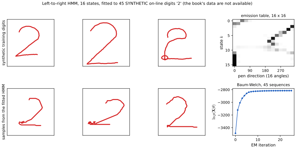
fig13_11. Download: PDF · SVG13.2.1 Maximum likelihood for the HMM
pp. 615–618 Given one observed sequence \(\mathbf{X}\), the likelihood is the joint (13.10) with the latent variables summed out:
\[ p(\mathbf{X}\given\bm\theta)=\sum_{\mathbf{Z}}p(\mathbf{X},\mathbf{Z}\given\bm\theta). \tag{13.11} \]Two difficulties. The sum has \(K^N\) terms, one per path through the lattice of Figure 13.7, and unlike a mixture for i.i.d. data it does not split into \(N\) separate sums over each \(\mathbf{z}_n\), because the factors \(p(\mathbf{z}_n\given\mathbf{z}_{n-1})\) tie neighbouring \(\mathbf{z}\)'s together. And even if it were evaluated, it is a sum over emission densities (a generalised mixture), so setting its derivatives to zero gives no closed form, exactly as for the Gaussian mixture of Section 9.2 (which is the special case with identical rows of \(\mathbf{A}\)). Both are solved by EM, with an E step computed by the recursions of Section 13.2.2.
The EM algorithm (Section 9.3; its monotonicity is proved in Section 9.4) alternates between computing the posterior \(p(\mathbf{Z}\given\mathbf{X},\bm\theta^{\rm old})\) and maximising
\[ Q(\bm\theta,\bm\theta^{\rm old})=\sum_{\mathbf{Z}}p(\mathbf{Z}\given\mathbf{X},\bm\theta^{\rm old})\ln p(\mathbf{X},\mathbf{Z}\given\bm\theta). \tag{13.12} \]Write \(\gamma\) for the posterior marginal of one latent variable and \(\xi\) for that of two successive ones:
\[ \gamma(\mathbf{z}_n)=p(\mathbf{z}_n\given\mathbf{X},\bm\theta^{\rm old}), \tag{13.13} \] \[ \xi(\mathbf{z}_{n-1},\mathbf{z}_n)=p(\mathbf{z}_{n-1},\mathbf{z}_n\given\mathbf{X},\bm\theta^{\rm old}). \tag{13.14} \]For each \(n\), \(\gamma(\mathbf{z}_n)\) is \(K\) nonnegative numbers summing to one and \(\xi(\mathbf{z}_{n-1},\mathbf{z}_n)\) a \(K\times K\) table summing to one. With \(\gamma(z_{nk})\) the value at \(z_{nk}=1\), and since the mean of a binary variable is the probability that it equals 1,
\[ \gamma(z_{nk})=\E[z_{nk}]=\sum_{\mathbf{z}_n}\gamma(\mathbf{z}_n)\,z_{nk}, \tag{13.15} \] \[ \xi(z_{n-1,j},z_{nk})=\E[z_{n-1,j}z_{nk}]=\sum_{\mathbf{z}_{n-1},\mathbf{z}_n}\xi(\mathbf{z}_{n-1},\mathbf{z}_n)\,z_{n-1,j}z_{nk}. \tag{13.16} \]Erratum. In some printings the rightmost expressions of (13.15) and (13.16) are written with \(\gamma(\mathbf{z})\) summed over the wrong variable; the forms above (sum over \(\mathbf{z}_n\) with \(\gamma(\mathbf{z}_n)\), and with \(\xi(\mathbf{z}_{n-1},\mathbf{z}_n)\) in (13.16)) are the corrected ones.
Result 13.6 (the expected complete-data log likelihood) pp. 616–617, (13.17)
For the HMM (13.10),
\[ Q(\bm\theta,\bm\theta^{\rm old})=\sum_{k=1}^{K}\gamma(z_{1k})\ln\pi_k+\sum_{n=2}^{N}\sum_{j=1}^{K}\sum_{k=1}^{K}\xi(z_{n-1,j},z_{nk})\ln A_{jk}+\sum_{n=1}^{N}\sum_{k=1}^{K}\gamma(z_{nk})\ln p(\mathbf{x}_n\given\bm\phi_k). \tag{13.17} \]So the E step needs only the \(NK\) numbers \(\gamma(z_{nk})\) and the \((N-1)K^2\) numbers \(\xi(z_{n-1,j},z_{nk})\), not the full posterior over \(K^N\) paths.
Derivation
Step 1: the log of the joint is linear in the indicators. Take logarithms in (13.10) and use (13.7)–(13.9):
\[ \ln p(\mathbf{X},\mathbf{Z}\given\bm\theta)=\sum_{k}z_{1k}\ln\pi_k+\sum_{n=2}^{N}\sum_{j,k}z_{n-1,j}z_{nk}\ln A_{jk}+\sum_{n=1}^{N}\sum_{k}z_{nk}\ln p(\mathbf{x}_n\given\bm\phi_k). \](When some \(A_{jk}=0\) the term \(z_{n-1,j}z_{nk}\ln A_{jk}\) is read as 0 if \(z_{n-1,j}z_{nk}=0\); configurations with \(z_{n-1,j}z_{nk}=1\) then have probability zero and do not contribute to (13.12).)
Step 2: take the posterior expectation. \(Q\) is the expectation of this expression under \(p(\mathbf{Z}\given\mathbf{X},\bm\theta^{\rm old})\). Expectation is linear, and \(\ln\pi_k\), \(\ln A_{jk}\), \(\ln p(\mathbf{x}_n\given\bm\phi_k)\) are constants (they depend on \(\bm\theta\) and the data, not on \(\mathbf{Z}\)), so \(Q\) is the same expression with each indicator replaced by its posterior mean: \(\E[z_{1k}]\), \(\E[z_{n-1,j}z_{nk}]\) and \(\E[z_{nk}]\).
Step 3: those means are \(\gamma\) and \(\xi\). The function \(z_{nk}\) depends on \(\mathbf{Z}\) only through \(\mathbf{z}_n\), so summing \(p(\mathbf{Z}\given\mathbf{X})z_{nk}\) over all other latent variables first gives \(\E[z_{nk}]\)
In the M step \(\gamma\) and \(\xi\) are held fixed and (13.17) is maximised over \(\bm\theta=\{\bm\pi,\mathbf{A},\bm\phi\}\). The three sums involve disjoint sets of parameters, so they are maximised separately. The book says the \(\bm\pi\) and \(\mathbf{A}\) updates are "easily achieved using appropriate Lagrange multipliers" (Exercise 13.5); here is the computation.
Result 13.7 (M step for the initial and transition probabilities; Exercise 13.5) p. 617, (13.18)–(13.19)
\[ \pi_k=\frac{\gamma(z_{1k})}{\sum_{j=1}^{K}\gamma(z_{1j})}, \tag{13.18} \] \[ A_{jk}=\frac{\sum_{n=2}^{N}\xi(z_{n-1,j},z_{nk})}{\sum_{l=1}^{K}\sum_{n=2}^{N}\xi(z_{n-1,j},z_{nl})}. \tag{13.19} \]Since \(\sum_j\gamma(z_{1j})=1\), (13.18) is just \(\pi_k=\gamma(z_{1k})\). Since \(\sum_l\xi(z_{n-1,j},z_{nl})=\gamma(z_{n-1,j})\), the denominator of (13.19) is \(\sum_{n=1}^{N-1}\gamma(z_{nj})\): \(A_{jk}\) is the expected number of \(j\to k\) transitions divided by the expected number of visits to \(j\) (excluding the last step, from which no transition is made). These are the global maximisers.
Derivation
Initial probabilities. Maximise \(F(\bm\pi)=\sum_kg_k\ln\pi_k\) with \(g_k=\gamma(z_{1k})\ge0\), subject to \(\sum_k\pi_k=1\) (Lagrange multipliers). The Lagrangian \(\sum_kg_k\ln\pi_k+\lambda(\sum_k\pi_k-1)\) has derivative \(g_k/\pi_k+\lambda\) in \(\pi_k\); setting it to zero gives \(\pi_k=-g_k/\lambda\). Summing over \(k\) and using the constraint, \(1=-\sum_kg_k/\lambda\), so \(\lambda=-\sum_jg_j\) and \(\pi_k=g_k/\sum_jg_j\), which is (13.18).
Why this is the maximum. \(F\) is a sum of concave functions \(g_k\ln\pi_k\) and the constraint set (the probability simplex) is convex, so a stationary point of the Lagrangian in the interior is the global maximum. A direct check, which also covers \(g_k=0\): with \(\hat\pi_k=g_k/G\), \(G=\sum_jg_j\), Gibbs' inequality (\(\KL(\hat{\bm\pi}\|\bm\pi)\ge0\), toolkit) gives \(\sum_k\hat\pi_k\ln\pi_k\)
Transition probabilities. The second term of (13.17) is \(\sum_j\big[\sum_kc_{jk}\ln A_{jk}\big]\) with \(c_{jk}=\sum_{n=2}^{N}\xi(z_{n-1,j},z_{nk})\). The constraints \(\sum_kA_{jk}=1\) act on each row separately, so each row \(j\) is an instance of the problem just solved, with \(g_k\) replaced by \(c_{jk}\) and one multiplier \(\lambda_j\) per row: \(A_{jk}=c_{jk}/\sum_lc_{jl}\), which is (13.19).
The simplified denominators. \(\gamma(\mathbf{z}_1)\) is a distribution, so \(\sum_j\gamma(z_{1j})=1\). Summing the pairwise marginal over its second argument gives the single marginal: \(\sum_l\xi(z_{n-1,j},z_{nl})\)
Result 13.8 (M step for Gaussian emissions; Exercise 13.7) pp. 617–618, (13.20)–(13.21)
If \(p(\mathbf{x}\given\bm\phi_k)\)
These are the Gaussian-mixture updates (9.24)–(9.25) with the responsibilities replaced by the posterior state probabilities \(\gamma(z_{nk})\), which now use the whole sequence.
Derivation
Only the last sum of (13.17) involves \(\bm\phi\), and with separate parameters per state it splits into one weighted Gaussian log likelihood per \(k\). With \(N_k=\sum_n\gamma(z_{nk})\) and dropping \(-\frac D2\ln2\pi\) terms,
\[ Q_k(\bm\mu_k,\bm\Sigma_k)=-\frac{N_k}{2}\ln|\bm\Sigma_k|-\frac12\sum_{n=1}^{N}\gamma(z_{nk})(\mathbf{x}_n-\bm\mu_k)^\T\bm\Sigma_k^{-1}(\mathbf{x}_n-\bm\mu_k). \]Mean. The gradient in \(\bm\mu_k\) (matrix calculus: \(\partial(\mathbf{a}^\T\mathbf{S}\mathbf{a})/\partial\mathbf{a}\)
Covariance. Put \(\bm\mu_k\) at (13.20) and write the quadratic form as a trace (toolkit): with \(\mathbf{S}_k\)
Using \(\partial\ln|\bm\Lambda|/\partial\bm\Lambda\)
Result 13.9 (M step for discrete and binary emissions; Exercise 13.8) p. 618, (13.22)–(13.23)
(a) If \(\mathbf{x}\) is a 1-of-\(D\) vector and in state \(k\) the symbol \(i\) has probability \(\mu_{ik}\) (\(\sum_i\mu_{ik}=1\)), then
\[ p(\mathbf{x}\given\mathbf{z})=\prod_{i=1}^{D}\prod_{k=1}^{K}\mu_{ik}^{\,x_iz_k}, \tag{13.22} \] \[ \mu_{ik}=\frac{\sum_{n=1}^{N}\gamma(z_{nk})\,x_{ni}}{\sum_{n=1}^{N}\gamma(z_{nk})}. \tag{13.23} \](b) If \(\mathbf{x}\) has \(D\) independent binary components with \(p(x_i=1\given z_k=1)=\mu_{ik}\), then \(p(\mathbf{x}\given\mathbf{z})\)
Derivation
(a) If \(z_k=1\) and \(x_i=1\), all exponents in (13.22) vanish except \(x_iz_k\), so the product is \(\mu_{ik}\), as required. The emission term of (13.17) becomes \(\sum_n\sum_k\gamma(z_{nk})\sum_ix_{ni}\ln\mu_{ik}\)
(b) The emission term is \(\sum_k\sum_i\sum_n\gamma(z_{nk})\{x_{ni}\ln\mu_{ik}\)
Result 13.10 (zeros are preserved by EM; Exercise 13.6) p. 617
If \(\pi_k=0\) or \(A_{jk}=0\) in \(\bm\theta^{\rm old}\), the same entry is zero after the M step, and hence at every later iteration. In particular a left-to-right structure (Figure 13.9) is kept automatically.
Proof
By (13.43) below, \(\xi(z_{n-1,j},z_{nk})\)
Initialisation pp. 617–618, 623. \(\bm\pi\) and \(\mathbf{A}\) are started uniformly or at random (respecting the constraints, and with the zeros that encode any structure); the emission parameters from a fit that ignores the order, for instance K-means or a Gaussian mixture fitted by EM to the data treated as i.i.d. (means from the cluster centres, covariances from the clusters). As in Chapter 9, the likelihood has many local maxima and the result depends on the start.
13.2.2 The forward-backward algorithm
pp. 618–625 The E step needs \(\gamma(\mathbf{z}_n)\) and \(\xi(\mathbf{z}_{n-1},\mathbf{z}_n)\). The graph of Figure 13.5 is a tree, so a two-pass message-passing algorithm computes them exactly; for the HMM it is called the forward-backward or Baum-Welch algorithm (Baum, 1972; Rabiner, 1989). The book first derives it with the sum and product rules plus eight conditional independence properties, then (Section 13.2.3) as the sum-product algorithm. Throughout this section the parameters are fixed at \(\bm\theta^{\rm old}\) and dropped from the notation, and the emission densities enter only through the numbers \(p(\mathbf{x}_n\given\mathbf{z}_n)\): nothing depends on whether \(\mathbf{x}\) is discrete or continuous.
The conditional independence properties
The book lists the following (Jordan, 2007), with \(\mathbf{X}=\{\mathbf{x}_1,\dots,\mathbf{x}_N\}\), and says they are "most easily proved using d-separation", leaving the details to the reader (Exercises 13.9 and 13.10).
\[ p(\mathbf{X}\given\mathbf{z}_n)=p(\mathbf{x}_1,\dots,\mathbf{x}_n\given\mathbf{z}_n)\,p(\mathbf{x}_{n+1},\dots,\mathbf{x}_N\given\mathbf{z}_n) \tag{13.24} \] \[ p(\mathbf{x}_1,\dots,\mathbf{x}_{n-1}\given\mathbf{x}_n,\mathbf{z}_n)=p(\mathbf{x}_1,\dots,\mathbf{x}_{n-1}\given\mathbf{z}_n) \tag{13.25} \] \[ p(\mathbf{x}_1,\dots,\mathbf{x}_{n-1}\given\mathbf{z}_{n-1},\mathbf{z}_n)=p(\mathbf{x}_1,\dots,\mathbf{x}_{n-1}\given\mathbf{z}_{n-1}) \tag{13.26} \] \[ p(\mathbf{x}_{n+1},\dots,\mathbf{x}_N\given\mathbf{z}_n,\mathbf{z}_{n+1})=p(\mathbf{x}_{n+1},\dots,\mathbf{x}_N\given\mathbf{z}_{n+1}) \tag{13.27} \] \[ p(\mathbf{x}_{n+2},\dots,\mathbf{x}_N\given\mathbf{z}_{n+1},\mathbf{x}_{n+1})=p(\mathbf{x}_{n+2},\dots,\mathbf{x}_N\given\mathbf{z}_{n+1}) \tag{13.28} \] \[ p(\mathbf{X}\given\mathbf{z}_{n-1},\mathbf{z}_n)=p(\mathbf{x}_1,\dots,\mathbf{x}_{n-1}\given\mathbf{z}_{n-1})\,p(\mathbf{x}_n\given\mathbf{z}_n)\,p(\mathbf{x}_{n+1},\dots,\mathbf{x}_N\given\mathbf{z}_n) \tag{13.29} \] \[ p(\mathbf{x}_{N+1}\given\mathbf{X},\mathbf{z}_{N+1})=p(\mathbf{x}_{N+1}\given\mathbf{z}_{N+1}) \tag{13.30} \] \[ p(\mathbf{z}_{N+1}\given\mathbf{z}_N,\mathbf{X})=p(\mathbf{z}_{N+1}\given\mathbf{z}_N) \tag{13.31} \](The last two concern the model extended by one step, \(N+1\) instead of \(N\).) All eight follow from one factorisation, proved first; then each is checked both algebraically and by d-separation. Erratum. In the sentence after (13.31) the book's "in the first of these results" should read "in the second of these results" (the argument given is for (13.25)).
Result 13.11 (cutting the chain at \(\mathbf{z}_n\); Exercise 13.10)
For the joint (13.6) and any \(1\le n\le N\), split the variables other than \(\mathbf{z}_n\) into the past \(\mathcal{P}_n\)
and \(p(\mathcal{F}_n\given\mathbf{z}_n)\)
Proof
Group the factors of (13.6):
\[ p(\mathbf{X},\mathbf{Z})=\underbrace{p(\mathbf{z}_1)\prod_{m=2}^{n}p(\mathbf{z}_m\given\mathbf{z}_{m-1})\prod_{m=1}^{n-1}p(\mathbf{x}_m\given\mathbf{z}_m)}_{g(\mathcal{P}_n,\,\mathbf{z}_n)}\;p(\mathbf{x}_n\given\mathbf{z}_n)\;\underbrace{\prod_{m=n+1}^{N}p(\mathbf{z}_m\given\mathbf{z}_{m-1})\,p(\mathbf{x}_m\given\mathbf{z}_m)}_{h(\mathcal{F}_n;\,\mathbf{z}_n)} . \]\(h\) sums to one over \(\mathcal{F}_n\) for every \(\mathbf{z}_n\). Sum over \(\mathbf{x}_N\) (only \(p(\mathbf{x}_N\given\mathbf{z}_N)\) contains it, and it sums to one), then over \(\mathbf{z}_N\) (only \(p(\mathbf{z}_N\given\mathbf{z}_{N-1})\) remains with it), then \(\mathbf{x}_{N-1}\), and so on down to \(\mathbf{z}_{n+1}\). The same peeling shows that summing the last pair \((\mathbf{x}_{N},\mathbf{z}_{N})\) out of the length-\(N\) model gives the length-\((N-1)\) model, which is the consistency statement.
\(g\) is the joint of \(\mathcal{P}_n\) and \(\mathbf{z}_n\). Summing the display over \(\mathcal{F}_n\) and \(\mathbf{x}_n\) removes \(h\) and \(p(\mathbf{x}_n\given\mathbf{z}_n)\), so \(p(\mathcal{P}_n,\mathbf{z}_n)\)
Conclusion. Dividing the display by \(p(\mathbf{z}_n)\): \(p(\mathcal{P}_n,\mathbf{x}_n,\mathcal{F}_n\given\mathbf{z}_n)\)
Result 13.12 (the eight properties; Exercises 13.9 and 13.10) p. 619, (13.24)–(13.31)
The joint (13.6) satisfies (13.24)–(13.31), and also (13.5).
Proof of each, algebraically (from Result 13.11) and by d-separation
Two facts are used repeatedly. (i) If \(\mathbf{a}\perp\!\!\!\perp\mathbf{b}\given\mathbf{c}\) then the same holds for any sub-collections of \(\mathbf{a}\) and \(\mathbf{b}\) (sum out the rest). (ii) If \((\mathbf{a},\mathbf{d})\perp\!\!\!\perp\mathbf{b}\given\mathbf{c}\), then \(\mathbf{a}\perp\!\!\!\perp\mathbf{b}\given(\mathbf{c},\mathbf{d})\): indeed \(p(\mathbf{a},\mathbf{b}\given\mathbf{c},\mathbf{d})\)
(13.24) Result 13.11 at \(n\): \(\mathbf{x}_{1:n}\) (part of \(\mathcal{P}_n\) together with \(\mathbf{x}_n\)) and \(\mathbf{x}_{n+1:N}\) (part of \(\mathcal{F}_n\)) are independent given \(\mathbf{z}_n\), by (i). d-separation: a path from \(\mathbf{x}_m\), \(m\le n\), to \(\mathbf{x}_{m'}\), \(m'\gt n\), runs \(\mathbf{x}_m\leftarrow\mathbf{z}_m\cdots\mathbf{z}_{m'}\)
(13.25) Result 13.11 at \(n\): \(\mathbf{x}_n\perp\!\!\!\perp\mathcal{P}_n\given\mathbf{z}_n\), so \(\mathbf{x}_{1:n-1}\perp\!\!\!\perp\mathbf{x}_n\given\mathbf{z}_n\), which is (13.25). d-separation: every path from \(\mathbf{x}_{1:n-1}\) to \(\mathbf{x}_n\) ends \(\mathbf{z}_{n-1}\to\mathbf{z}_n\to\mathbf{x}_n\), head-to-tail at the observed \(\mathbf{z}_n\).
(13.26) Result 13.11 at \(n-1\): \(\mathcal{P}_{n-1}\cup\{\mathbf{x}_{n-1}\}\) is independent of \(\mathcal{F}_{n-1}\ni\mathbf{z}_n\) given \(\mathbf{z}_{n-1}\); by (i), \(\mathbf{x}_{1:n-1}\perp\!\!\!\perp\mathbf{z}_n\given\mathbf{z}_{n-1}\), which is (13.26). d-separation: paths from \(\mathbf{x}_m\), \(m\le n-1\), to \(\mathbf{z}_n\) pass \(\mathbf{z}_{n-1}\) head-to-tail (tail-to-tail when \(m=n-1\)), and \(\mathbf{z}_{n-1}\) is observed.
(13.27) Result 13.11 at \(n+1\): \(\mathcal{P}_{n+1}\ni\mathbf{z}_n\) is independent of \((\mathbf{x}_{n+1},\mathcal{F}_{n+1})\supset\mathbf{x}_{n+1:N}\) given \(\mathbf{z}_{n+1}\). d-separation: paths from \(\mathbf{z}_n\) to \(\mathbf{x}_{m}\), \(m\gt n\), pass \(\mathbf{z}_{n+1}\) head-to-tail, observed.
(13.28) Result 13.11 at \(n+1\): \(\mathbf{x}_{n+1}\perp\!\!\!\perp\mathcal{F}_{n+1}\given\mathbf{z}_{n+1}\), and \(\mathbf{x}_{n+2:N}\subset\mathcal{F}_{n+1}\). d-separation: paths from \(\mathbf{x}_{n+1}\) to \(\mathbf{x}_m\), \(m\ge n+2\), start \(\mathbf{x}_{n+1}\leftarrow\mathbf{z}_{n+1}\)
(13.29) Result 13.11 at \(n\) with (i): \((\mathbf{x}_{1:n-1},\mathbf{z}_{n-1})\), \(\mathbf{x}_n\) and \(\mathbf{x}_{n+1:N}\) are mutually independent given \(\mathbf{z}_n\). Hence
\[ p(\mathbf{X},\mathbf{z}_{n-1}\given\mathbf{z}_n)=p(\mathbf{x}_{1:n-1},\mathbf{z}_{n-1}\given\mathbf{z}_n)\,p(\mathbf{x}_n\given\mathbf{z}_n)\,p(\mathbf{x}_{n+1:N}\given\mathbf{z}_n). \]Divide by \(p(\mathbf{z}_{n-1}\given\mathbf{z}_n)\): \(p(\mathbf{X}\given\mathbf{z}_{n-1},\mathbf{z}_n)\)
(13.30) In the chain of length \(N+1\) (which marginalises to the given one, by the consistency part of Result 13.11), Result 13.11 at \(n=N+1\) gives \(\mathbf{x}_{N+1}\perp\!\!\!\perp\mathcal{P}_{N+1}\given\mathbf{z}_{N+1}\), and \(\mathbf{X}\subset\mathcal{P}_{N+1}\). d-separation: paths from \(\mathbf{X}\) to \(\mathbf{x}_{N+1}\) end \(\mathbf{z}_N\)
(13.31) Result 13.11 at \(n=N\) in the chain of length \(N+1\): \((\mathcal{P}_N,\mathbf{x}_N)\) is independent of \(\mathcal{F}_N\)
(13.5) Result 13.11 at \(n\): \(\mathbf{z}_{n-1}\in\mathcal{P}_n\) and \(\mathbf{z}_{n+1}\in\mathcal{F}_n\). ∎
The forward recursion
By Bayes' theorem and (13.24),
\[ \gamma(\mathbf{z}_n)=p(\mathbf{z}_n\given\mathbf{X})=\frac{p(\mathbf{X}\given\mathbf{z}_n)\,p(\mathbf{z}_n)}{p(\mathbf{X})} \tag{13.32} \] \[ \gamma(\mathbf{z}_n)=\frac{p(\mathbf{x}_1,\dots,\mathbf{x}_n,\mathbf{z}_n)\,p(\mathbf{x}_{n+1},\dots,\mathbf{x}_N\given\mathbf{z}_n)}{p(\mathbf{X})}=\frac{\alpha(\mathbf{z}_n)\,\beta(\mathbf{z}_n)}{p(\mathbf{X})} \tag{13.33} \](in the middle, \(p(\mathbf{x}_{1:n}\given\mathbf{z}_n)p(\mathbf{z}_n)\)
\(\alpha(\mathbf{z}_n)\) is the joint probability of the data so far and the current state; \(\beta(\mathbf{z}_n)\) the probability of the future data given the current state. Each is a vector of \(K\) numbers, \(\alpha(z_{nk})\) and \(\beta(z_{nk})\). The denominator \(p(\mathbf{X})\) is the likelihood at \(\bm\theta^{\rm old}\).
Result 13.13 (the \(\alpha\) recursion) pp. 620–621, (13.36)–(13.37)
\[ \alpha(\mathbf{z}_n)=p(\mathbf{x}_n\given\mathbf{z}_n)\sum_{\mathbf{z}_{n-1}}\alpha(\mathbf{z}_{n-1})\,p(\mathbf{z}_n\given\mathbf{z}_{n-1}), \tag{13.36} \] \[ \alpha(\mathbf{z}_1)=p(\mathbf{x}_1,\mathbf{z}_1)=p(\mathbf{z}_1)\,p(\mathbf{x}_1\given\mathbf{z}_1)=\prod_{k=1}^{K}\big\{\pi_k\,p(\mathbf{x}_1\given\bm\phi_k)\big\}^{z_{1k}}. \tag{13.37} \]In components, \(\alpha(z_{nk})\)
Derivation, with the reason for each step
\[ \begin{aligned} \alpha(\mathbf{z}_n)&=p(\mathbf{x}_1,\dots,\mathbf{x}_n,\mathbf{z}_n) &&\text{definition (13.34)}\\ &=p(\mathbf{x}_1,\dots,\mathbf{x}_n\given\mathbf{z}_n)\,p(\mathbf{z}_n) &&\text{product rule}\\ &=p(\mathbf{x}_n\given\mathbf{z}_n)\,p(\mathbf{x}_1,\dots,\mathbf{x}_{n-1}\given\mathbf{z}_n)\,p(\mathbf{z}_n) &&\text{product rule and (13.25)}\\ &=p(\mathbf{x}_n\given\mathbf{z}_n)\,p(\mathbf{x}_1,\dots,\mathbf{x}_{n-1},\mathbf{z}_n) &&\text{product rule}\\ &=p(\mathbf{x}_n\given\mathbf{z}_n)\sum_{\mathbf{z}_{n-1}}p(\mathbf{x}_1,\dots,\mathbf{x}_{n-1},\mathbf{z}_{n-1},\mathbf{z}_n) &&\text{sum rule}\\ &=p(\mathbf{x}_n\given\mathbf{z}_n)\sum_{\mathbf{z}_{n-1}}p(\mathbf{x}_1,\dots,\mathbf{x}_{n-1},\mathbf{z}_n\given\mathbf{z}_{n-1})\,p(\mathbf{z}_{n-1}) &&\text{product rule}\\ &=p(\mathbf{x}_n\given\mathbf{z}_n)\sum_{\mathbf{z}_{n-1}}p(\mathbf{x}_1,\dots,\mathbf{x}_{n-1}\given\mathbf{z}_{n-1})\,p(\mathbf{z}_n\given\mathbf{z}_{n-1})\,p(\mathbf{z}_{n-1}) &&\text{product rule and (13.26)}\\ &=p(\mathbf{x}_n\given\mathbf{z}_n)\sum_{\mathbf{z}_{n-1}}p(\mathbf{x}_1,\dots,\mathbf{x}_{n-1},\mathbf{z}_{n-1})\,p(\mathbf{z}_n\given\mathbf{z}_{n-1}) &&\text{product rule} \end{aligned} \]and the last sum contains \(\alpha(\mathbf{z}_{n-1})\) by (13.34), which is (13.36). In the third line, the product rule gives \(p(\mathbf{x}_{1:n}\given\mathbf{z}_n)\)
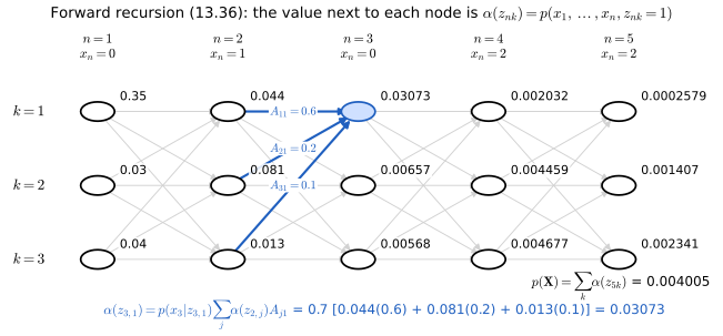
fig13_12. Download: PDF · SVGThe backward recursion
Result 13.14 (the \(\beta\) recursion) pp. 621–622, (13.38)–(13.39)
\[ \beta(\mathbf{z}_n)=\sum_{\mathbf{z}_{n+1}}\beta(\mathbf{z}_{n+1})\,p(\mathbf{x}_{n+1}\given\mathbf{z}_{n+1})\,p(\mathbf{z}_{n+1}\given\mathbf{z}_n), \tag{13.38} \]started from \(\beta(\mathbf{z}_N)=1\) for every value of \(\mathbf{z}_N\). In components, \(\beta(z_{nj})\)
Derivation, with the reason for each step
\[ \begin{aligned} \beta(\mathbf{z}_n)&=p(\mathbf{x}_{n+1},\dots,\mathbf{x}_N\given\mathbf{z}_n) &&\text{definition (13.35)}\\ &=\sum_{\mathbf{z}_{n+1}}p(\mathbf{x}_{n+1},\dots,\mathbf{x}_N,\mathbf{z}_{n+1}\given\mathbf{z}_n) &&\text{sum rule}\\ &=\sum_{\mathbf{z}_{n+1}}p(\mathbf{x}_{n+1},\dots,\mathbf{x}_N\given\mathbf{z}_n,\mathbf{z}_{n+1})\,p(\mathbf{z}_{n+1}\given\mathbf{z}_n) &&\text{product rule}\\ &=\sum_{\mathbf{z}_{n+1}}p(\mathbf{x}_{n+1},\dots,\mathbf{x}_N\given\mathbf{z}_{n+1})\,p(\mathbf{z}_{n+1}\given\mathbf{z}_n) &&\text{(13.27)}\\ &=\sum_{\mathbf{z}_{n+1}}p(\mathbf{x}_{n+2},\dots,\mathbf{x}_N\given\mathbf{z}_{n+1})\,p(\mathbf{x}_{n+1}\given\mathbf{z}_{n+1})\,p(\mathbf{z}_{n+1}\given\mathbf{z}_n) &&\text{product rule and (13.28)} \end{aligned} \]and the first factor is \(\beta(\mathbf{z}_{n+1})\) by (13.35). In the last line \(p(\mathbf{x}_{n+1:N}\given\mathbf{z}_{n+1})\)
The starting value (13.39). At \(n=N\), (13.33) with the definition of \(\alpha\) reads
\[ p(\mathbf{z}_N\given\mathbf{X})=\frac{p(\mathbf{X},\mathbf{z}_N)\,\beta(\mathbf{z}_N)}{p(\mathbf{X})}, \tag{13.39} \]and the left-hand side equals \(p(\mathbf{X},\mathbf{z}_N)/p(\mathbf{X})\) by Bayes' theorem. So (13.33) holds at \(n=N\) exactly when \(\beta(\mathbf{z}_N)=1\). This is also what (13.35) means when the set of future observations is empty (the probability of observing nothing is one), and with it (13.38) at \(n=N-1\) gives \(\beta(\mathbf{z}_{N-1})\)
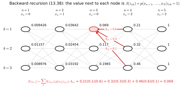
fig13_13. Download: PDF · SVGPosterior marginals and the likelihood
Result 13.15 (\(\gamma\), \(\xi\) and \(p(\mathbf{X})\) from \(\alpha\) and \(\beta\)) pp. 622–623, (13.40)–(13.43)
(a) \(\gamma(\mathbf{z}_n)\)
(c) The pairwise posterior is
\[ \xi(\mathbf{z}_{n-1},\mathbf{z}_n)=\frac{\alpha(\mathbf{z}_{n-1})\,p(\mathbf{x}_n\given\mathbf{z}_n)\,p(\mathbf{z}_n\given\mathbf{z}_{n-1})\,\beta(\mathbf{z}_n)}{p(\mathbf{X})}, \tag{13.43} \]that is \(\xi(z_{n-1,j},z_{nk})\)
Derivation
(b) Sum (13.33) over \(\mathbf{z}_n\): the left side sums to one because \(\gamma\) is a distribution, so \(p(\mathbf{X})\)
(c) By Bayes' theorem and then (13.29),
\[ \xi(\mathbf{z}_{n-1},\mathbf{z}_n)=\frac{p(\mathbf{X}\given\mathbf{z}_{n-1},\mathbf{z}_n)\,p(\mathbf{z}_{n-1},\mathbf{z}_n)}{p(\mathbf{X})}=\frac{p(\mathbf{x}_{1:n-1}\given\mathbf{z}_{n-1})\,p(\mathbf{x}_n\given\mathbf{z}_n)\,p(\mathbf{x}_{n+1:N}\given\mathbf{z}_n)\,p(\mathbf{z}_n\given\mathbf{z}_{n-1})\,p(\mathbf{z}_{n-1})}{p(\mathbf{X})}, \]and \(p(\mathbf{x}_{1:n-1}\given\mathbf{z}_{n-1})p(\mathbf{z}_{n-1})\)
(d) Substitute (13.33) into (13.20): the common factor \(1/p(\mathbf{X})\) cancels between numerator and denominator. The same happens in (13.18), (13.19), (13.21) and (13.23). Typo. The book prints the upper limits of the sums in (13.40) as \(n\); they are \(N\). ∎
Result 13.16 (cost: linear in \(N\) instead of exponential) pp. 621, 623
Given the \(NK\) emission values, the forward pass, the backward pass and the computation of all \(\gamma\) and \(\xi\) cost \(O(K^2N)\) operations and \(O(KN)\) memory (plus \(O(K^2)\) at a time for \(\xi\), which can be accumulated into the M-step sums as it is produced). Direct evaluation of (13.11) costs about \(NK^N\).
Proof
One step of (13.36) computes, for each of the \(K\) values of \(k\), a sum of \(K\) products \(\alpha(z_{n-1,j})A_{jk}\) and one more multiplication: \(K^2+K\) multiplications and \(K(K-1)\) additions, so \(O(K^2)\) per step and \(O(K^2N)\) for the chain. (13.38) is the same. \(\gamma\) costs \(K\) multiplications per step, and \(\xi\) has \(K^2\) entries per step, each a product of four stored numbers. Direct evaluation of (13.11) sums \(K^N\) terms, each a product of about \(2N\) factors. For example, with \(K=3\) and \(N=100\), \(K^N\approx5\times10^{47}\), against about \(2\cdot9\cdot100\) multiply-adds per pass. The saving comes from the distributive law: in \(\sum_{\mathbf{z}_1}\cdots\sum_{\mathbf{z}_N}\prod(\cdots)\) each \(\mathbf{z}_n\) appears in only two neighbouring transition factors, so the sums can be pushed inside the product one at a time, and \(\alpha(\mathbf{z}_n)\) is exactly the partial sum over all paths that end in a given state at time \(n\). ∎
Algorithm 13.1 (EM for the HMM: the Baum-Welch algorithm) pp. 623–624
- Initialise \(\bm\pi\), \(\mathbf{A}\) (uniform or random, with structural zeros) and \(\bm\phi\) (e.g. from K-means).
- E step. Compute the emission values \(p(\mathbf{x}_n\given\bm\phi_k)\). Run the forward recursion (13.36)–(13.37) and the backward recursion (13.38) from \(\beta(\mathbf{z}_N)=1\), in their scaled form (Algorithm 13.2) in practice. Form \(\gamma\) by (13.33) and \(\xi\) by (13.43), and the log likelihood by (13.42) or (13.63).
- M step. Update \(\bm\pi\), \(\mathbf{A}\) by (13.18)–(13.19) and the emission parameters by (13.20)–(13.21) (Gaussian) or (13.23) (discrete or binary).
- Repeat 2–3 until the increase of the log likelihood falls below a threshold. The log likelihood never decreases (EM, Section 9.4).
In the course code, Baum-Welch on 300 observations from the model of Figure 13.8, started at random, raised the log likelihood from \(-170.9\) to \(732.7\) without a single decrease. Likewise EM for the linear dynamical system of Section 13.3.2 raised it from \(-931.4\) to \(-635.1\) on simulated data, above the value \(-643.4\) at the true parameters (maximum likelihood fits the sample, so it beats the truth).
Several sequences p. 624; Exercise 13.12. Maximum likelihood works when the training sequence is long compared with the number of parameters. Otherwise use \(R\) independent sequences \(\mathbf{X}^{(r)}\): the complete-data log likelihood is a sum over \(r\), so the E step runs forward-backward on each sequence separately, and the M step sums the expected counts over sequences as well as over \(n\), (13.124)–(13.126) (see Exercise 13.12). This matters most for left-to-right models, in which an off-diagonal transition occurs at most once per sequence.
The predictive distribution
Result 13.17 (one-step prediction) pp. 624–625, (13.44)
\[ p(\mathbf{x}_{N+1}\given\mathbf{X})=\frac{1}{p(\mathbf{X})}\sum_{\mathbf{z}_{N+1}}p(\mathbf{x}_{N+1}\given\mathbf{z}_{N+1})\sum_{\mathbf{z}_N}p(\mathbf{z}_{N+1}\given\mathbf{z}_N)\,\alpha(\mathbf{z}_N). \tag{13.44} \]So the whole past enters only through the \(K\) numbers \(\alpha(\mathbf{z}_N)/p(\mathbf{X})\)
Derivation, with the reason for each step
\[ \begin{aligned} p(\mathbf{x}_{N+1}\given\mathbf{X})&=\sum_{\mathbf{z}_{N+1}}p(\mathbf{x}_{N+1},\mathbf{z}_{N+1}\given\mathbf{X}) &&\text{sum rule}\\ &=\sum_{\mathbf{z}_{N+1}}p(\mathbf{x}_{N+1}\given\mathbf{z}_{N+1})\,p(\mathbf{z}_{N+1}\given\mathbf{X}) &&\text{product rule and (13.30)}\\ &=\sum_{\mathbf{z}_{N+1}}p(\mathbf{x}_{N+1}\given\mathbf{z}_{N+1})\sum_{\mathbf{z}_N}p(\mathbf{z}_{N+1},\mathbf{z}_N\given\mathbf{X}) &&\text{sum rule}\\ &=\sum_{\mathbf{z}_{N+1}}p(\mathbf{x}_{N+1}\given\mathbf{z}_{N+1})\sum_{\mathbf{z}_N}p(\mathbf{z}_{N+1}\given\mathbf{z}_N)\,p(\mathbf{z}_N\given\mathbf{X}) &&\text{product rule and (13.31)}\\ &=\sum_{\mathbf{z}_{N+1}}p(\mathbf{x}_{N+1}\given\mathbf{z}_{N+1})\sum_{\mathbf{z}_N}p(\mathbf{z}_{N+1}\given\mathbf{z}_N)\,\frac{p(\mathbf{z}_N,\mathbf{X})}{p(\mathbf{X})} &&\text{definition of conditional} \end{aligned} \]and \(p(\mathbf{z}_N,\mathbf{X})=\alpha(\mathbf{z}_N)\) by (13.34). The new step is part of the chain of length \(N+1\); by the consistency in Result 13.11 its marginal over the first \(N\) steps is the original model, so \(p(\mathbf{X})\), \(\alpha(\mathbf{z}_N)\) and \(p(\mathbf{z}_N\given\mathbf{X})\) are unchanged by adding it. ∎
(The errata note that on p. 624 the book should refer to (13.30), not (13.29), for this derivation.)
Priors and Bayesian HMMs p. 625. A prior \(p(\bm\theta)\) turns maximum likelihood into MAP estimation: the E step is unchanged and the M step maximises \(Q+\ln p(\bm\theta)\). For example, independent Dirichlet priors \(\Dir(\mathbf{a}_j)\) on the rows of \(\mathbf{A}\) add \(\sum_k(a_{jk}-1)\ln A_{jk}\) to the \(j\)-th row of (13.17), and the argument of Result 13.7 gives \(A_{jk}\)
13.2.3 The sum-product algorithm for the HMM
pp. 625–627 The graph of the HMM is a tree, so the sum-product algorithm of Section 8.4.4 computes all the local marginals exactly; for this graph it is the forward-backward algorithm, and it delivers the \(\alpha\)-\(\beta\) recursions with almost no work. First convert the directed graph into a factor graph (Figure 13.14): one factor \(\chi(\mathbf{z}_1)=p(\mathbf{z}_1)\), one factor \(\psi_n(\mathbf{z}_{n-1},\mathbf{z}_n)\)
Because we always condition on the observed \(\mathbf{x}_1,\dots,\mathbf{x}_N\), each \(g_n\) is a function of \(\mathbf{z}_n\) alone and can be absorbed into a neighbouring factor. This gives the simplified chain of Figure 13.15 with factors
\[ h(\mathbf{z}_1)=p(\mathbf{z}_1)\,p(\mathbf{x}_1\given\mathbf{z}_1), \tag{13.45} \] \[ f_n(\mathbf{z}_{n-1},\mathbf{z}_n)=p(\mathbf{z}_n\given\mathbf{z}_{n-1})\,p(\mathbf{x}_n\given\mathbf{z}_n), \tag{13.46} \]whose product \(h(\mathbf{z}_1)\prod_{n=2}^Nf_n(\mathbf{z}_{n-1},\mathbf{z}_n)\) is \(p(\mathbf{X},\mathbf{Z})\) as a function of \(\mathbf{Z}\), i.e. the unnormalised posterior \(p(\mathbf{Z}\given\mathbf{X})\,p(\mathbf{X})\).
Result 13.18 (forward-backward is sum-product; Exercises 13.11, 13.13 and 13.14) pp. 626–627, (13.47)–(13.54)
Take \(\mathbf{z}_N\) as the root. The sum-product messages on the chain of Figure 13.15 are
\[ \mu_{\mathbf{z}_{n-1}\to f_n}(\mathbf{z}_{n-1})=\mu_{f_{n-1}\to\mathbf{z}_{n-1}}(\mathbf{z}_{n-1}), \tag{13.47} \] \[ \mu_{f_n\to\mathbf{z}_n}(\mathbf{z}_n)=\sum_{\mathbf{z}_{n-1}}f_n(\mathbf{z}_{n-1},\mathbf{z}_n)\,\mu_{\mathbf{z}_{n-1}\to f_n}(\mathbf{z}_{n-1}), \tag{13.48} \] \[ \mu_{f_n\to\mathbf{z}_n}(\mathbf{z}_n)=\sum_{\mathbf{z}_{n-1}}f_n(\mathbf{z}_{n-1},\mathbf{z}_n)\,\mu_{f_{n-1}\to\mathbf{z}_{n-1}}(\mathbf{z}_{n-1}), \tag{13.49} \] \[ \alpha(\mathbf{z}_n)=\mu_{f_n\to\mathbf{z}_n}(\mathbf{z}_n), \tag{13.50} \] \[ \mu_{f_{n+1}\to\mathbf{z}_n}(\mathbf{z}_n)=\sum_{\mathbf{z}_{n+1}}f_{n+1}(\mathbf{z}_n,\mathbf{z}_{n+1})\,\mu_{f_{n+2}\to\mathbf{z}_{n+1}}(\mathbf{z}_{n+1}), \tag{13.51} \] \[ \beta(\mathbf{z}_n)=\mu_{f_{n+1}\to\mathbf{z}_n}(\mathbf{z}_n), \tag{13.52} \](with \(\mu_{f_1\to\mathbf{z}_1}\) read as \(\mu_{h\to\mathbf{z}_1}=h\) and \(\mu_{f_{N+1}\to\mathbf{z}_N}\) as 1), and the marginals are
\[ p(\mathbf{z}_n,\mathbf{X})=\mu_{f_n\to\mathbf{z}_n}(\mathbf{z}_n)\,\mu_{f_{n+1}\to\mathbf{z}_n}(\mathbf{z}_n)=\alpha(\mathbf{z}_n)\,\beta(\mathbf{z}_n), \tag{13.53} \] \[ \gamma(\mathbf{z}_n)=\frac{p(\mathbf{z}_n,\mathbf{X})}{p(\mathbf{X})}=\frac{\alpha(\mathbf{z}_n)\beta(\mathbf{z}_n)}{p(\mathbf{X})}, \tag{13.54} \]and \(\xi(\mathbf{z}_{n-1},\mathbf{z}_n)\) is (13.43). The messages defined in (13.50) and (13.52) are the same functions as \(\alpha\) and \(\beta\) defined by (13.34)–(13.35).
Erratum. In (13.51) the book writes the message indices with \(f\) to the right of the arrow; they are \(\mu_{f_{n+1}\to\mathbf{z}_n}\) and \(\mu_{f_{n+2}\to\mathbf{z}_{n+1}}\), as above.
Derivation
The message rules. From Chapter 8, a factor sends \(\mu_{f\to x}(x)\)
Forward messages. \(\mathbf{z}_{n-1}\) has two neighbours, \(f_{n-1}\) and \(f_n\), so its message to \(f_n\) is the single message from \(f_{n-1}\): (13.47) (variable nodes "perform no computation"). Factor \(f_n\) has neighbours \(\mathbf{z}_{n-1}\), \(\mathbf{z}_n\), so (8.66) gives (13.48), and substituting (13.47) gives (13.49). With (13.46) and (13.50) this is \(\alpha(\mathbf{z}_n)\)
The message is \(\alpha\) by definition, too (Exercise 13.13). By (8.64), the message from \(f_n\) to \(\mathbf{z}_n\) is the sum, over all variables in the part of the tree on the \(f_n\) side of \(\mathbf{z}_n\), of the product of all factors in that part:
\[ \mu_{f_n\to\mathbf{z}_n}(\mathbf{z}_n)=\sum_{\mathbf{z}_1,\dots,\mathbf{z}_{n-1}}h(\mathbf{z}_1)\prod_{m=2}^{n}f_m(\mathbf{z}_{m-1},\mathbf{z}_m)=\sum_{\mathbf{z}_1,\dots,\mathbf{z}_{n-1}}p(\mathbf{x}_{1:n},\mathbf{z}_{1:n})=p(\mathbf{x}_{1:n},\mathbf{z}_n), \]where the middle equality is (13.6) for the first \(n\) steps (the marginal of the chain, Result 13.11) and the last is the sum rule. That is (13.34).
Backward messages (Exercise 13.14). Messages from the root \(\mathbf{z}_N\) back to the leaf: \(\mathbf{z}_N\) has the single neighbour \(f_N\), so it sends \(\mu_{\mathbf{z}_N\to f_N}=1\) (8.70), which is \(\beta(\mathbf{z}_N)=1\). Each \(\mathbf{z}_{n+1}\) passes on what it receives from \(f_{n+2}\), and \(f_{n+1}\) applies (8.66): (13.51). With (13.46), \(\beta(\mathbf{z}_n)\)
by Result 13.11 (the product is \(p(\mathcal{F}_n\given\mathbf{z}_n)\)), which is (13.35).
Marginals. By (8.63) the marginal of a variable node is the product of all incoming messages. The function represented by the factor graph is \(p(\mathbf{X},\mathbf{Z})\), so this "marginal" is \(\sum_{\mathbf{Z}\setminus\mathbf{z}_n}p(\mathbf{X},\mathbf{Z})\)
Pairwise marginal (Exercise 13.11). By (8.72), the marginal of the variables of factor \(f_n\) is the factor times the messages arriving at it: \(p(\mathbf{z}_{n-1},\mathbf{z}_n,\mathbf{X})\)
13.2.4 Scaling factors
pp. 627–629 The recursion (13.36) multiplies at each step by numbers \(p(\mathbf{z}_n\given\mathbf{z}_{n-1})\) and \(p(\mathbf{x}_n\given\mathbf{z}_n)\) that are typically much smaller than one, so \(\alpha(\mathbf{z}_n)\)
Result 13.19 (the scaled forward recursion) pp. 627–628, (13.55)–(13.59)
Define the filtered distribution and the scaling factors
\[ \widehat\alpha(\mathbf{z}_n)=p(\mathbf{z}_n\given\mathbf{x}_1,\dots,\mathbf{x}_n)=\frac{\alpha(\mathbf{z}_n)}{p(\mathbf{x}_1,\dots,\mathbf{x}_n)}, \tag{13.55} \] \[ c_n=p(\mathbf{x}_n\given\mathbf{x}_1,\dots,\mathbf{x}_{n-1})\qquad(c_1=p(\mathbf{x}_1)). \tag{13.56} \]Then
\[ p(\mathbf{x}_1,\dots,\mathbf{x}_n)=\prod_{m=1}^{n}c_m, \tag{13.57} \] \[ \alpha(\mathbf{z}_n)=p(\mathbf{z}_n\given\mathbf{x}_1,\dots,\mathbf{x}_n)\,p(\mathbf{x}_1,\dots,\mathbf{x}_n)=\Big(\prod_{m=1}^{n}c_m\Big)\widehat\alpha(\mathbf{z}_n), \tag{13.58} \] \[ c_n\,\widehat\alpha(\mathbf{z}_n)=p(\mathbf{x}_n\given\mathbf{z}_n)\sum_{\mathbf{z}_{n-1}}\widehat\alpha(\mathbf{z}_{n-1})\,p(\mathbf{z}_n\given\mathbf{z}_{n-1}), \tag{13.59} \]and \(c_n\) is the number that normalises the right-hand side of (13.59) to sum to one over \(\mathbf{z}_n\). At \(n=1\): \(c_1\widehat\alpha(\mathbf{z}_1)\)
Derivation
(13.57) is the product rule applied repeatedly: \(p(\mathbf{x}_{1:n})\)
and divide by \(\prod_{m=1}^{n-1}c_m\gt0\): (13.59). Summing (13.59) over \(\mathbf{z}_n\), and using \(\sum_{\mathbf{z}_n}\widehat\alpha(\mathbf{z}_n)\)
Result 13.20 (the scaled backward recursion and the marginals; Exercise 13.15) pp. 628, (13.60)–(13.65)
Define \(\widehat\beta(\mathbf{z}_n)\) by
\[ \beta(\mathbf{z}_n)=\Big(\prod_{m=n+1}^{N}c_m\Big)\widehat\beta(\mathbf{z}_n). \tag{13.60} \]Then
\[ \widehat\beta(\mathbf{z}_n)=\frac{p(\mathbf{x}_{n+1},\dots,\mathbf{x}_N\given\mathbf{z}_n)}{p(\mathbf{x}_{n+1},\dots,\mathbf{x}_N\given\mathbf{x}_1,\dots,\mathbf{x}_n)}, \tag{13.61} \] \[ c_{n+1}\,\widehat\beta(\mathbf{z}_n)=\sum_{\mathbf{z}_{n+1}}\widehat\beta(\mathbf{z}_{n+1})\,p(\mathbf{x}_{n+1}\given\mathbf{z}_{n+1})\,p(\mathbf{z}_{n+1}\given\mathbf{z}_n), \tag{13.62} \]with \(\widehat\beta(\mathbf{z}_N)=1\), and
\[ p(\mathbf{X})=\prod_{n=1}^{N}c_n,\qquad \ln p(\mathbf{X})=\sum_{n=1}^{N}\ln c_n, \tag{13.63} \] \[ \gamma(\mathbf{z}_n)=\widehat\alpha(\mathbf{z}_n)\,\widehat\beta(\mathbf{z}_n), \tag{13.64} \] \[ \xi(\mathbf{z}_{n-1},\mathbf{z}_n)=c_n^{-1}\,\widehat\alpha(\mathbf{z}_{n-1})\,p(\mathbf{x}_n\given\mathbf{z}_n)\,p(\mathbf{z}_n\given\mathbf{z}_{n-1})\,\widehat\beta(\mathbf{z}_n). \tag{13.65} \]Erratum. Some printings have \(c_n\) instead of \(c_n^{-1}\), and \(\mathbf{z}_{-1}\) instead of \(\mathbf{z}_{n-1}\), on the right of (13.65).
Derivation
(13.61). By (13.57), \(\prod_{m=n+1}^{N}c_m\)
(13.62). Substitute (13.60) at \(n\) and \(n+1\) into (13.38):
\[ \Big(\prod_{m=n+1}^{N}c_m\Big)\widehat\beta(\mathbf{z}_n)=\sum_{\mathbf{z}_{n+1}}\Big(\prod_{m=n+2}^{N}c_m\Big)\widehat\beta(\mathbf{z}_{n+1})\,p(\mathbf{x}_{n+1}\given\mathbf{z}_{n+1})\,p(\mathbf{z}_{n+1}\given\mathbf{z}_n), \]and divide by \(\prod_{m=n+2}^{N}c_m\). At \(n=N\) the product in (13.60) is empty (equal to 1), so \(\widehat\beta(\mathbf{z}_N)\)
(13.63) is (13.57) at \(n=N\). (13.64). Substitute (13.58) and (13.60) into (13.33): \(\gamma(\mathbf{z}_n)\)
Algorithm 13.2 (scaled forward-backward) pp. 627–628
- Forward. \(\mathbf{a}\)
\({}=(\pi_kp(\mathbf{x}_1\given\bm\phi_k))_k\), \(c_1=\sum_k a_k\), \(\widehat{\bm\alpha}_1=\mathbf{a}/c_1\). For \(n=2,\dots,N\): \(\mathbf{a}\) \({}=(\widehat{\bm\alpha}_{n-1}\mathbf{A})\odot\mathbf{e}_n\), \(c_n=\sum_ka_k\), \(\widehat{\bm\alpha}_n=\mathbf{a}/c_n\). - Log likelihood. \(\ln p(\mathbf{X})=\sum_n\ln c_n\) (13.63).
- Backward. \(\widehat{\bm\beta}_N=\mathbf{1}\). For \(n=N-1,\dots,1\): \(\widehat{\bm\beta}_n\)
\({}=\mathbf{A}(\mathbf{e}_{n+1}\odot\widehat{\bm\beta}_{n+1})/c_{n+1}\). - Marginals. \(\gamma(z_{nk})\)
\({}=\widehat\alpha_{nk}\widehat\beta_{nk}\); \(\xi(z_{n-1,j},z_{nk})\) \({}=\widehat\alpha_{n-1,j}A_{jk}e_{nk}\widehat\beta_{nk}/c_n\).
Checks worth coding: each \(\gamma(\mathbf{z}_n)\) sums to one, and \(\sum_j\xi(z_{n-1,j},z_{nk})=\gamma(z_{nk})\). On a short sequence, \(\gamma\), \(\xi\) and \(p(\mathbf{X})\) agree with brute-force enumeration of all \(K^N\) paths (I checked this to machine precision for \(K=3\), \(N=7\) with Gaussian emissions).
An alternative that the book does not pursue is to run (13.36) in the log domain, \(\ln\alpha(z_{nk})\)
Result 13.21 (the \(\alpha\)-\(\gamma\) form of the backward pass) p. 629
Instead of \(\widehat\beta\), the backward pass can propagate \(\gamma\) itself:
\[ \gamma(\mathbf{z}_n)=\sum_{\mathbf{z}_{n+1}}\frac{\widehat\alpha(\mathbf{z}_n)\,p(\mathbf{z}_{n+1}\given\mathbf{z}_n)}{\sum_{\mathbf{z}_n'}\widehat\alpha(\mathbf{z}_n')\,p(\mathbf{z}_{n+1}\given\mathbf{z}_n')}\,\gamma(\mathbf{z}_{n+1}),\qquad\gamma(\mathbf{z}_N)=\widehat\alpha(\mathbf{z}_N), \]and the fraction is \(p(\mathbf{z}_n\given\mathbf{z}_{n+1},\mathbf{X})\)
Derivation
A conditional independence. Result 13.11 at \(n+1\) says \(\mathcal{P}_{n+1}\)
Its value. By Bayes' theorem, \(p(\mathbf{z}_n\given\mathbf{z}_{n+1},\mathbf{x}_{1:n})\)
The recursion. \(\gamma(\mathbf{z}_n)\)
13.2.5 The Viterbi algorithm
pp. 629–631 Often the hidden states mean something (phonemes in speech, regions of a gene) and we want the single most probable state sequence, \(\argmax_{\mathbf{Z}}p(\mathbf{Z}\given\mathbf{X})\)
Result 13.22 (the Viterbi recursion; Exercise 13.16) pp. 629–630, (13.66)–(13.70)
With \(\mathbf{z}_N\) as root, the max-sum messages on the chain of Figure 13.15 are
\[ \mu_{\mathbf{z}_n\to f_{n+1}}(\mathbf{z}_n)=\mu_{f_n\to\mathbf{z}_n}(\mathbf{z}_n), \tag{13.66} \] \[ \mu_{f_{n+1}\to\mathbf{z}_{n+1}}(\mathbf{z}_{n+1})=\max_{\mathbf{z}_n}\big\{\ln f_{n+1}(\mathbf{z}_n,\mathbf{z}_{n+1})+\mu_{\mathbf{z}_n\to f_{n+1}}(\mathbf{z}_n)\big\}. \tag{13.67} \]Writing \(\omega(\mathbf{z}_n)\)
and \(\omega\) has the meaning
\[ \omega(\mathbf{z}_n)=\max_{\mathbf{z}_1,\dots,\mathbf{z}_{n-1}}\ln p(\mathbf{x}_1,\dots,\mathbf{x}_n,\mathbf{z}_1,\dots,\mathbf{z}_n). \tag{13.70} \]In particular \(\max_{\mathbf{z}_N}\omega(\mathbf{z}_N)\)
Derivation, directly from the joint (Exercise 13.16), and from max-sum
Two rules for maxima. (R1) If \(a\) does not depend on \(u\), \(\max_u\{a+g(u)\}=a+\max_ug(u)\). (R2) Maxima over several variables can be taken one at a time: \(\max_{u,v}g(u,v)=\max_u\max_vg(u,v)\). Together they let a maximisation be pushed past every term that does not involve the variable, exactly as the distributive law pushes sums past factors (with \((\max,+)\) in place of \((+,\times)\)).
Recursion. Define \(\omega\) by (13.70). For \(n\ge2\), the joint of the first \(n\) steps factorises as \(p(\mathbf{x}_{1:n},\mathbf{z}_{1:n})\)
which is (13.68) with \(n\) in place of \(n+1\). At \(n=1\) there is nothing to maximise and \(\omega(\mathbf{z}_1)\)
As max-sum. In max-sum (8.93)–(8.94) a factor sends \(\max\) over its other variables of \(\ln f\) plus incoming messages, and a variable sends the sum of messages from its other neighbours. A variable node \(\mathbf{z}_n\) on the chain has one other neighbour, so it passes its message on unchanged: (13.66). Factor \(f_{n+1}\) then sends (13.67). Eliminating (13.66) and using \(\ln f_{n+1}\)
Back-tracking pp. 630–631, (13.71). The recursion gives the probability of the best path but not the path. During the forward pass, for each \(n\ge2\) and each state \(k\) of \(\mathbf{z}_n\), record which state of \(\mathbf{z}_{n-1}\) achieved the maximum:
\[ \psi_n(k)=\argmax_{j}\big\{\ln A_{jk}+\omega(z_{n-1,j})\big\}. \]Then set \(k_N^{\max}=\argmax_k\omega(z_{Nk})\) and trace back:
\[ k_{n-1}^{\max}=\psi_n(k_n^{\max}),\qquad n=N,N-1,\dots,2. \tag{13.71} \](The book writes the function without the index \(n\); it depends on \(n\) through \(\omega(\mathbf{z}_{n-1})\) and the emissions. Erratum: some printings have a garbled (13.71); the form above is the corrected one.)
Algorithm 13.3 (Viterbi) pp. 629–631
- \(\omega_{1k}\)
\({}=\ln\pi_k+\ln p(\mathbf{x}_1\given\bm\phi_k)\) for \(k=1,\dots,K\). - For \(n=2,\dots,N\) and each \(k\): \(\psi_n(k)=\argmax_j\{\omega_{n-1,j}+\ln A_{jk}\}\) and \(\omega_{nk}\)
\({}=\ln p(\mathbf{x}_n\given\bm\phi_k)\) \({}+\omega_{n-1,\psi_n(k)}+\ln A_{\psi_n(k),k}\). - \(k_N=\argmax_k\omega_{Nk}\); then \(k_{n-1}=\psi_n(k_n)\) for \(n=N,\dots,2\). Output the path \((k_1,\dots,k_N)\) and \(\max_{\mathbf{Z}}\ln p(\mathbf{X},\mathbf{Z})\)
\({}=\omega_{N,k_N}\).
Cost \(O(K^2N)\) time and \(O(KN)\) memory for the pointers \(\psi\). Zero transition probabilities give \(\ln A_{jk}=-\infty\), which simply excludes those predecessors.
Why back-tracking returns a most probable path
Claim: for every \(n\) and \(k\), the path \(\mathbf{z}^{(n,k)}\) obtained by setting \(z_n=k\) and following the pointers back attains the maximum in (13.70) for \(\mathbf{z}_n=k\), i.e. \(\ln p(\mathbf{x}_{1:n},\mathbf{z}^{(n,k)})\)
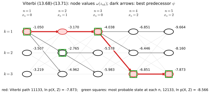
fig13_16. Download: PDF · SVGResult 13.23 (most probable path versus most probable states) p. 629
(a) The Viterbi path maximises the probability that the whole state sequence is correct, \(p(\widehat{\mathbf{Z}}=\mathbf{Z}\given\mathbf{X})\). The sequence \(\widehat z_n=\argmax_k\gamma(z_{nk})\) maximises the expected number of correct states, \(\E\big[\sum_n1\{\widehat{\mathbf{z}}_n=\mathbf{z}_n\}\given\mathbf{X}\big]\)
(b) Example. \(K=3\) states, \(\bm\pi=(\frac13,\frac13,\frac13)\), three observation symbols \(a,b,c\), and
\[ \mathbf{A}=\begin{pmatrix}0.75&0&0.25\\0&1&0\\0&1&0\end{pmatrix}, \] \[ \mathbf{B}=\big(p(\text{symbol}\given\text{state})\big)=\begin{pmatrix}0.40&0.5&0.10\\0.35&0.5&0.15\\0.25&0.5&0.25\end{pmatrix}, \]with observations \(\mathbf{X}=(a,b)\). The posterior over the nine paths is
| \(\mathbf{z}_1\backslash\mathbf{z}_2\) | 1 | 2 | 3 | \(\gamma(\mathbf{z}_1)\) |
|---|---|---|---|---|
| 1 | 0.30 | 0 | 0.10 | 0.40 |
| 2 | 0 | 0.35 | 0 | 0.35 |
| 3 | 0 | 0.25 | 0 | 0.25 |
| \(\gamma(\mathbf{z}_2)\) | 0.30 | 0.60 | 0.10 |
The individually most probable states are \(\widehat z_1=1\) (probability 0.40) and \(\widehat z_2=2\) (0.60), but the path \((1,2)\) has posterior probability zero, since \(A_{12}=0\). The Viterbi path is \((2,2)\), with posterior probability 0.35.
Proof and the numbers
(a) For a fixed guess \(\widehat{\mathbf{Z}}\), the probability that it is entirely right is \(p(\mathbf{Z}=\widehat{\mathbf{Z}}\given\mathbf{X})\), maximised by the posterior mode, which Viterbi finds. The expected number of correct positions is, by linearity, \(\sum_n p(\mathbf{z}_n=\widehat{\mathbf{z}}_n\given\mathbf{X})\)
(b) The joint is \(p(\mathbf{X},z_1=i,z_2=j)\)
13.2.6 Extensions of the hidden Markov model
pp. 631–635 The basic HMM and maximum likelihood training have been extended in many directions; the graphical-model view makes it easy to see which extensions keep exact inference cheap.
Discriminative training
The digit samples of Figure 13.11 show that an HMM can be a poor generative model. If the goal is to classify sequences, it can pay to train the class models discriminatively. With \(R\) training sequences \(\mathbf{X}_r\) labelled by classes \(m_r\in\{1,\dots,M\}\), one HMM \(\bm\theta_m\) per class and class priors \(p(m)\), maximise the conditional log likelihood (cross-entropy)
\[ \sum_{r=1}^{R}\ln p(m_r\given\mathbf{X}_r) \tag{13.72} \] \[ =\sum_{r=1}^{R}\ln\left\{\frac{p(\mathbf{X}_r\given\bm\theta_{m_r})\,p(m_r)}{\sum_{l=1}^{M}p(\mathbf{X}_r\given\bm\theta_l)\,p(l)}\right\}. \tag{13.73} \]Filling the gap 13.1: the gradient of the discriminative criterion pp. 631–632, (13.73)
The book only says that optimising (13.73) "is more complex than for maximum likelihood" and needs every sequence evaluated under every model. Here is the gradient that a gradient-based optimiser would use, and how forward-backward supplies it.
Derivation
Outer layer. Write \(L_{rl}=\ln p(\mathbf{X}_r\given\bm\theta_l)\) and \(P_{rl}\)
Sequences of class \(m\) push \(\bm\theta_m\) up the likelihood, weighted by how badly they are currently classified; sequences of other classes push it down, weighted by how much model \(m\) wrongly claims them. So every sequence must be run through every model (to get \(P_{rm}\)), as the book says.
Inner layer (Fisher's identity). For any latent-variable model, \(\frac{\partial}{\partial\bm\theta}\ln p(\mathbf{X}\given\bm\theta)\)
State durations
Result 13.24 (HMM state durations are geometric) p. 632, (13.74)
The probability that a sequence sampled from an HMM spends exactly \(T\) further steps in state \(k\) before leaving it is
\[ p(T)=(A_{kk})^T(1-A_{kk})\propto\exp(T\ln A_{kk}), \tag{13.74} \]a geometric distribution decaying exponentially in \(T\) (\(\ln A_{kk}\lt0\)). The total time spent in state \(k\) per visit, \(T+1\), has mean \(1/(1-A_{kk})\). Erratum. Some printings have a spurious minus sign in the exponent on the right of (13.74).
Proof
Given \(\mathbf{z}_n=k\), by the Markov property the next transitions are independent draws from row \(k\) of \(\mathbf{A}\): stay with probability \(A_{kk}\), leave with probability \(1-A_{kk}\). "Stay exactly \(T\) more steps, then leave" has probability \(A_{kk}^T(1-A_{kk})\), and \(A_{kk}^T=\exp(T\ln A_{kk})\). Summing, \(\sum_{T\ge0}A_{kk}^T(1-A_{kk})=1\), and \(\E[T+1]\)
The most likely duration is always the shortest one, which is unrealistic for, say, phonemes, which have a typical length. The fix is a semi-Markov (explicit-duration) model: set \(A_{kk}=0\), give each state a duration distribution \(p(T\given k)\), and on entering \(k\) draw \(T\) and emit \(T\) observations, usually independently, \(\prod_{t=1}^{T}p(\mathbf{x}_t\given k)\). Forward-backward and EM carry over with an extra sum over the length of the current segment (Rabiner, 1989), costing about \(O(K^2ND_{\max})\) for durations up to \(D_{\max}\).
Autoregressive and input-output HMMs
Long-range correlations between observations can only pass through the hidden chain. The autoregressive HMM (Ephraim et al., 1989) adds links from earlier observations, so \(\mathbf{x}_n\) depends on \(\mathbf{z}_n\) and on \(\mathbf{x}_{n-1},\mathbf{x}_{n-2}\) (Figure 13.17); for Gaussian emissions, \(p(\mathbf{x}_n\given\mathbf{z}_n=k,\mathbf{x}_{n-1},\mathbf{x}_{n-2})\) is a linear-Gaussian regression with state-dependent coefficients, fitted in the M step by weighted least squares. The input-output HMM (Bengio and Frasconi, 1996) adds an observed input sequence \(\mathbf{u}_1,\dots,\mathbf{u}_N\) that influences the transitions, the emissions or both (Figure 13.18): a model for supervised learning of sequence-to-sequence maps, trained by maximising \(p(\mathbf{X}\given\mathbf{U},\bm\theta)\).
Result 13.25 (the autoregressive and input-output HMMs keep linear-time inference; Exercises 13.17 and 13.18) pp. 632–633
In both models, with all observed variables given, (a) the latent chain keeps the Markov property (13.5): \(\mathbf{z}_{n+1}\perp\!\!\!\perp\mathbf{z}_{n-1}\given\mathbf{z}_n\) and the observed variables; (b) the posterior over \(\mathbf{Z}\) has the HMM form, with factors
\[ h(\mathbf{z}_1)=p(\mathbf{z}_1\given\mathbf{u}_1)\,p(\mathbf{x}_1\given\mathbf{z}_1,\mathbf{u}_1),\qquad f_n(\mathbf{z}_{n-1},\mathbf{z}_n)=p(\mathbf{z}_n\given\mathbf{z}_{n-1},\mathbf{u}_n)\,p(\mathbf{x}_n\given\mathbf{z}_n,\mathbf{u}_n) \]for the input-output HMM, and \(h(\mathbf{z}_1)\)
with \(\alpha(\mathbf{z}_n)\)
Proof
Factor graph (Exercise 13.17). The joint of the input-output HMM (conditional on \(\mathbf{U}\)) is \(p(\mathbf{X},\mathbf{Z}\given\mathbf{U})\)
Markov property. The posterior \(p(\mathbf{Z}\given\mathbf{X},\mathbf{U})\)
Recursions (Exercise 13.18). Apply the sum-product derivation of Result 13.18 to the factors \(h,f_n\): the forward message is \(\alpha(\mathbf{z}_n)\)
Factorial HMMs
A factorial HMM (Ghahramani and Jordan, 1997) has \(M\) independent latent Markov chains \(\mathbf{z}^{(1)},\dots,\mathbf{z}^{(M)}\), and \(\mathbf{x}_n\) depends on all of \(\mathbf{z}_n^{(1)},\dots,\mathbf{z}_n^{(M)}\) (Figure 13.19); for continuous \(\mathbf{x}\) a natural emission is \(\N(\mathbf{x}_n\given\sum_m\mathbf{W}^{(m)}\mathbf{z}_n^{(m)},\bm\Sigma)\). The appeal is representational: 10 bits of state need \(K=2^{10}=1024\) states in one chain, but only 10 binary chains. The M step is straightforward; the E step is the problem.
Result 13.26 (exact inference in a factorial HMM is exponential in the number of chains) pp. 634–635
Let each of \(M\) chains have \(K\) states. (a) Given \(\mathbf{X}\), the chains are not independent, and a single chain is not even Markov on its own (Figure 13.20). (b) The model is an ordinary HMM on the combined state \(\mathbf{s}_n\)
Proof
(a) \(\mathbf{x}_n\) is a common child of \(\mathbf{z}_n^{(1)}\) and \(\mathbf{z}_n^{(2)}\), observed: the path \(\mathbf{z}_n^{(1)}\)
(b) The joint is \(\prod_m\big[p(\mathbf{z}_1^{(m)})\prod_np(\mathbf{z}_n^{(m)}\given\mathbf{z}_{n-1}^{(m)})\big]\)
(c) \(\alpha(\mathbf{s}_n)\)
Approximations are therefore used: Gibbs sampling (Chapter 11), or variational inference (Section 10.1) with either a fully factorised \(q\) or, better, a structured \(q\) made of \(M\) independent Markov chains. In the structured case the variational updates run an ordinary forward-backward pass along each chain separately, with emission terms replaced by expectations under the other chains, at cost \(O(NMK^2)\) per sweep, while keeping the correlations within each chain (Ghahramani and Jordan, 1997). The broader lesson of the section: graphical models suggest many structures, d-separation tells which ones keep exact inference tractable, and variational or sampling methods handle the rest.
13.3 Linear dynamical systems
pp. 635–637 A motivating problem. A sensor returns the value of a quantity \(z\) plus zero-mean Gaussian noise. If \(z\) is constant, averaging many readings beats any single one. If \(z\) changes in time, averaging all readings blurs the change, while using only the latest reading keeps all its noise; a window of recent readings, or a weighted average favouring recent ones, is a compromise, but its width or weights have to be guessed. A probabilistic model of how \(z\) evolves and how it is measured settles the question: the optimal weighting comes out of inference. The model used is the linear dynamical system (LDS): the state space model of Figure 13.5 with continuous latent variables and linear-Gaussian conditionals.
Why Gaussian? For inference to stay linear in \(N\), the forward message must keep its functional form: taking \(\widehat\alpha(\mathbf{z}_{n-1})\), multiplying by \(p(\mathbf{z}_n\given\mathbf{z}_{n-1})\) and \(p(\mathbf{x}_n\given\mathbf{z}_n)\) and integrating out \(\mathbf{z}_{n-1}\) must give a distribution of the same family, with new parameters. Linear-Gaussian conditionals have this closure property (Result 13.27); a mixture-of-Gaussians emission does not, since the number of components then multiplies by \(K\) at every step (Filling the gap 13.2). Just as the HMM extends the mixture models of Chapter 9 to sequences, the LDS extends the continuous latent variable models of Chapter 12 (probabilistic PCA, factor analysis): each pair \((\mathbf{z}_n,\mathbf{x}_n)\) is a linear-Gaussian latent variable model, but the \(\mathbf{z}_n\) now form a Markov chain. HMMs and linear dynamical systems were developed independently; as graphical models they are the same structure with discrete or Gaussian states. The forward recursion is the Kalman filter (Kalman, 1960), the backward one the Kalman smoother or Rauch-Tung-Striebel (RTS) equations (Rauch et al., 1965).
Definition 13.3 (linear dynamical system) p. 637, (13.75)–(13.83)
Latent \(\mathbf{z}_n\in\R^M\), observed \(\mathbf{x}_n\in\R^D\), with
\[ p(\mathbf{z}_n\given\mathbf{z}_{n-1})=\N(\mathbf{z}_n\given\mathbf{A}\mathbf{z}_{n-1},\bm\Gamma), \tag{13.75} \] \[ p(\mathbf{x}_n\given\mathbf{z}_n)=\N(\mathbf{x}_n\given\mathbf{C}\mathbf{z}_n,\bm\Sigma), \tag{13.76} \] \[ p(\mathbf{z}_1)=\N(\mathbf{z}_1\given\bm\mu_0,\mathbf{P}_0), \tag{13.77} \]and joint distribution (13.6). Equivalently, as noisy linear equations,
\[ \mathbf{z}_n=\mathbf{A}\mathbf{z}_{n-1}+\mathbf{w}_n \tag{13.78} \] \[ \mathbf{x}_n=\mathbf{C}\mathbf{z}_n+\mathbf{v}_n \tag{13.79} \] \[ \mathbf{z}_1=\bm\mu_0+\mathbf{u} \tag{13.80} \]with all noise terms independent of each other and over time,
\[ \mathbf{w}\sim\N(\mathbf{w}\given\mathbf{0},\bm\Gamma) \tag{13.81} \] \[ \mathbf{v}\sim\N(\mathbf{v}\given\mathbf{0},\bm\Sigma) \tag{13.82} \] \[ \mathbf{u}\sim\N(\mathbf{u}\given\mathbf{0},\mathbf{P}_0). \tag{13.83} \]The parameters are \(\bm\theta\)
Erratum. In some printings the initial covariance is written \(\mathbf{V}_0\) in (13.77)–(13.110) and the related exercises; it is \(\mathbf{P}_0\) throughout.
The equivalence of the two forms: if \(\mathbf{z}_{n-1}\) is given, \(\mathbf{A}\mathbf{z}_{n-1}+\mathbf{w}_n\) is a constant plus \(\N(\mathbf{0},\bm\Gamma)\) noise, which is (13.75), and independence of the noises over time gives exactly the conditional independences of Figure 13.5.
Result 13.27 (everything is Gaussian) pp. 636–638
(a) The joint distribution of \((\mathbf{z}_1,\dots,\mathbf{z}_N,\mathbf{x}_1,\dots,\mathbf{x}_N)\) is Gaussian, so every marginal and conditional of it is Gaussian; in particular \(p(\mathbf{z}_n\given\mathbf{x}_{1:n})\), \(p(\mathbf{z}_n\given\mathbf{X})\) and \(p(\mathbf{z}_{n-1},\mathbf{z}_n\given\mathbf{X})\). (b) Its moments are \(\E[\mathbf{z}_n]=\mathbf{A}^{n-1}\bm\mu_0\), \(\cov[\mathbf{z}_n]=\mathbf{S}_n\) with \(\mathbf{S}_1=\mathbf{P}_0\), \(\mathbf{S}_n\)
Proof
Unrolling (13.78)–(13.80), \(\mathbf{z}_n\)
So, in principle, all inference in an LDS is "condition a big Gaussian" with the formulas of Section 2.3, at cost \(O((N(M+D))^3)\). The Kalman filter and smoother do the same computation in \(O(N(M^3+D^3))\) by exploiting the chain structure. (I checked that the filter and smoother below reproduce the means and covariances obtained by conditioning the full joint Gaussian, to machine precision, on a random two-dimensional example.)
Result 13.28 (no Viterbi needed; Exercise 13.19) p. 637
In an LDS the sequence of individually most probable states, \(\argmax_{\mathbf{z}_n}p(\mathbf{z}_n\given\mathbf{X})\) for each \(n\), is the jointly most probable state sequence \(\argmax_{\mathbf{Z}}p(\mathbf{Z}\given\mathbf{X})\). Both equal the smoothed means \(\widehat{\bm\mu}_n\).
Proof
By Result 13.27, \(p(\mathbf{Z}\given\mathbf{X})\) is a Gaussian with some mean \(\mathbf{m}=(\mathbf{m}_1,\dots,\mathbf{m}_N)\). A Gaussian density is largest at its mean (the quadratic form in the exponent is zero there and positive elsewhere), so the joint mode is \(\mathbf{m}\). The marginal of the block \(\mathbf{z}_n\) is Gaussian with mean \(\mathbf{m}_n\), the corresponding block of \(\mathbf{m}\) (the marginal of a partitioned Gaussian keeps its sub-vector of the mean, (2.98)), so its mode is \(\mathbf{m}_n\). Hence the marginal modes, put together, are the joint mode. For the HMM this fails (Result 13.23) because a discrete distribution has no such structure. ∎
13.3.1 Inference in LDS
pp. 638–641 The LDS has the same factorisation (13.6) and factor graphs (Figures 13.14, 13.15) as the HMM, so the same algorithms apply with sums over \(\mathbf{z}_n\) replaced by integrals. Every argument of Sections 13.2.2–13.2.4 used only the sum and product rules and the factorisation, so it holds verbatim for densities. By convention the forward messages are the normalised filtered distributions, the analogue of the scaled \(\widehat\alpha\) of (13.59):
\[ \widehat\alpha(\mathbf{z}_n)=\N(\mathbf{z}_n\given\bm\mu_n,\mathbf{V}_n), \tag{13.84} \] \[ c_n\widehat\alpha(\mathbf{z}_n)=p(\mathbf{x}_n\given\mathbf{z}_n)\int\widehat\alpha(\mathbf{z}_{n-1})\,p(\mathbf{z}_n\given\mathbf{z}_{n-1})\,\d\mathbf{z}_{n-1}. \tag{13.85} \]Substituting (13.75), (13.76) and (13.84),
\[ c_n\N(\mathbf{z}_n\given\bm\mu_n,\mathbf{V}_n)=\N(\mathbf{x}_n\given\mathbf{C}\mathbf{z}_n,\bm\Sigma)\int\N(\mathbf{z}_n\given\mathbf{A}\mathbf{z}_{n-1},\bm\Gamma)\,\N(\mathbf{z}_{n-1}\given\bm\mu_{n-1},\mathbf{V}_{n-1})\,\d\mathbf{z}_{n-1}. \tag{13.86} \]Given \(\bm\mu_{n-1},\mathbf{V}_{n-1}\) and the new \(\mathbf{x}_n\), the task is to find \(\bm\mu_n,\mathbf{V}_n\) and \(c_n\). It splits into a prediction step (the integral) and an update step (multiplication by the emission density and normalisation).
Result 13.29 (the prediction step; Exercise 13.20) pp. 638–639, (13.87)–(13.88)
\[ \int\N(\mathbf{z}_n\given\mathbf{A}\mathbf{z}_{n-1},\bm\Gamma)\,\N(\mathbf{z}_{n-1}\given\bm\mu_{n-1},\mathbf{V}_{n-1})\,\d\mathbf{z}_{n-1}=\N(\mathbf{z}_n\given\mathbf{A}\bm\mu_{n-1},\mathbf{P}_{n-1}), \tag{13.87} \] \[ \mathbf{P}_{n-1}=\mathbf{A}\mathbf{V}_{n-1}\mathbf{A}^\T+\bm\Gamma. \tag{13.88} \]This is the one-step predictive distribution \(p(\mathbf{z}_n\given\mathbf{x}_{1:n-1})\).
Derivation (two ways)
From the linear-Gaussian result. Result T.15 (the book's (2.115)): if \(p(\mathbf{x})\)
From the noise equation. If \(\mathbf{z}_{n-1}\)
Why it is the prediction. Under the posterior given \(\mathbf{x}_{1:n-1}\), \(\mathbf{z}_{n-1}\)
Result 13.30 (the Kalman filter update; Exercise 13.21) p. 639, (13.89)–(13.92)
With the Kalman gain
\[ \mathbf{K}_n=\mathbf{P}_{n-1}\mathbf{C}^\T\big(\mathbf{C}\mathbf{P}_{n-1}\mathbf{C}^\T+\bm\Sigma\big)^{-1}, \tag{13.92} \] \[ \bm\mu_n=\mathbf{A}\bm\mu_{n-1}+\mathbf{K}_n(\mathbf{x}_n-\mathbf{C}\mathbf{A}\bm\mu_{n-1}) \tag{13.89} \] \[ \mathbf{V}_n=(\mathbf{I}-\mathbf{K}_n\mathbf{C})\mathbf{P}_{n-1} \tag{13.90} \] \[ c_n=\N(\mathbf{x}_n\given\mathbf{C}\mathbf{A}\bm\mu_{n-1},\ \mathbf{C}\mathbf{P}_{n-1}\mathbf{C}^\T+\bm\Sigma). \tag{13.91} \]Innovation form. With the innovation (prediction error) \(\mathbf{e}_n\)
and, equivalently, \(\mathbf{V}_n\)
Derivation by completing the square
Write \(\mathbf{m}=\mathbf{A}\bm\mu_{n-1}\), \(\mathbf{P}=\mathbf{P}_{n-1}\) and \(\mathbf{x}=\mathbf{x}_n\). By (13.86)–(13.87), as functions of \(\mathbf{z}=\mathbf{z}_n\),
\[ c_n\N(\mathbf{z}\given\bm\mu_n,\mathbf{V}_n)=\N(\mathbf{x}\given\mathbf{C}\mathbf{z},\bm\Sigma)\,\N(\mathbf{z}\given\mathbf{m},\mathbf{P}). \]Step 1: the exponent. The logarithm of the right-hand side is, up to terms not involving \(\mathbf{z}\),
\[ -\tfrac12(\mathbf{x}-\mathbf{C}\mathbf{z})^\T\bm\Sigma^{-1}(\mathbf{x}-\mathbf{C}\mathbf{z})-\tfrac12(\mathbf{z}-\mathbf{m})^\T\mathbf{P}^{-1}(\mathbf{z}-\mathbf{m})=-\tfrac12\mathbf{z}^\T\big(\mathbf{P}^{-1}+\mathbf{C}^\T\bm\Sigma^{-1}\mathbf{C}\big)\mathbf{z}+\mathbf{z}^\T\big(\mathbf{P}^{-1}\mathbf{m}+\mathbf{C}^\T\bm\Sigma^{-1}\mathbf{x}\big)+\const \](expand both quadratics; the cross terms \(-\frac12(-2\mathbf{z}^\T\mathbf{C}^\T\bm\Sigma^{-1}\mathbf{x})\) and \(-\frac12(-2\mathbf{z}^\T\mathbf{P}^{-1}\mathbf{m})\) give the linear term). By completing the square, a density whose log is \(-\frac12\mathbf{z}^\T\mathbf{Q}\mathbf{z}\)
(This is also Result T.15, the book's (2.116), with \(\bm\Lambda=\mathbf{P}^{-1}\), \(\mathbf{L}=\bm\Sigma^{-1}\), \(\mathbf{A}\to\mathbf{C}\), \(\mathbf{b}=\mathbf{0}\).)
Step 2: the covariance in gain form. The Woodbury identity (C.7), \((\mathbf{P}^{-1}+\mathbf{C}^\T\bm\Sigma^{-1}\mathbf{C})^{-1}\)
Step 3: the gain identity (C.5). \(\mathbf{V}_n\mathbf{C}^\T\bm\Sigma^{-1}\)
Step 4: the mean. From Step 2, \(\mathbf{V}_n\mathbf{P}^{-1}\)
which is (13.89).
Step 5: the normaliser. Integrate both sides of the first display over \(\mathbf{z}\): the left gives \(c_n\), the right the marginal of \(\mathbf{x}\) in the linear-Gaussian model, \(\N(\mathbf{x}\given\mathbf{C}\mathbf{m},\bm\Sigma+\mathbf{C}\mathbf{P}\mathbf{C}^\T)\) (Result T.15 again): (13.91). As in (13.56), \(c_n=p(\mathbf{x}_n\given\mathbf{x}_{1:n-1})\); since \(\mathbf{e}_n\) is \(\mathbf{x}_n\) minus a function of \(\mathbf{x}_{1:n-1}\), it is \(\N(\mathbf{0},\mathbf{S}_n)\) given the past.
Joseph form. Expand \((\mathbf{I}-\mathbf{K}\mathbf{C})\mathbf{P}(\mathbf{I}-\mathbf{K}\mathbf{C})^\T\)
Result 13.31 (the first step; Exercises 13.22 and 13.23) p. 639, (13.93)–(13.97)
The recursion starts from
\[ c_1\widehat\alpha(\mathbf{z}_1)=p(\mathbf{z}_1)\,p(\mathbf{x}_1\given\mathbf{z}_1), \tag{13.93} \]which gives
\[ \bm\mu_1=\bm\mu_0+\mathbf{K}_1(\mathbf{x}_1-\mathbf{C}\bm\mu_0) \tag{13.94} \] \[ \mathbf{V}_1=(\mathbf{I}-\mathbf{K}_1\mathbf{C})\mathbf{P}_0 \tag{13.95} \] \[ c_1=\N(\mathbf{x}_1\given\mathbf{C}\bm\mu_0,\ \mathbf{C}\mathbf{P}_0\mathbf{C}^\T+\bm\Sigma) \tag{13.96} \] \[ \mathbf{K}_1=\mathbf{P}_0\mathbf{C}^\T\big(\mathbf{C}\mathbf{P}_0\mathbf{C}^\T+\bm\Sigma\big)^{-1}. \tag{13.97} \]Derivation
(13.93) is the definition \(\widehat\alpha(\mathbf{z}_1)\)
Algorithm 13.4 (the Kalman filter) pp. 638–639
- Initialise the prediction for step 1: \(\mathbf{m}_1=\bm\mu_0\), \(\mathbf{P}=\mathbf{P}_0\).
- For \(n=1,\dots,N\):
- Predict (for \(n\ge2\)): \(\mathbf{m}_n=\mathbf{A}\bm\mu_{n-1}\), \(\mathbf{P}_{n-1}\)
\({}=\mathbf{A}\mathbf{V}_{n-1}\mathbf{A}^\T\) \({}+\bm\Gamma\). - Innovation: \(\mathbf{e}_n=\mathbf{x}_n-\mathbf{C}\mathbf{m}_n\), \(\mathbf{S}_n\)
\({}=\mathbf{C}\mathbf{P}_{n-1}\mathbf{C}^\T\) \({}+\bm\Sigma\) (with \(\mathbf{P}_0\) when \(n=1\)). - Update: \(\mathbf{K}_n\)
\({}=\mathbf{P}_{n-1}\mathbf{C}^\T\mathbf{S}_n^{-1}\), \(\bm\mu_n=\mathbf{m}_n+\mathbf{K}_n\mathbf{e}_n\), \(\mathbf{V}_n\) \({}=(\mathbf{I}-\mathbf{K}_n\mathbf{C})\mathbf{P}_{n-1}\). - Likelihood: add \(\ln c_n\)
\({}=-\frac12\{D\ln2\pi+\ln|\mathbf{S}_n|\) \({}+\mathbf{e}_n^\T\mathbf{S}_n^{-1}\mathbf{e}_n\}\).
- Predict (for \(n\ge2\)): \(\mathbf{m}_n=\mathbf{A}\bm\mu_{n-1}\), \(\mathbf{P}_{n-1}\)
- Missing observation at step \(n\): skip (b)–(d), so \(\bm\mu_n=\mathbf{m}_n\), \(\mathbf{V}_n=\mathbf{P}_{n-1}\) (the emission factor is absent from (13.85), and \(c_n=1\)).
Cost per step: \(O(M^3+D^3+M^2D+MD^2)\), dominated by the \(D\times D\) inverse (solve) and the \(M\times M\) products.
Interpretation pp. 639–640. \(\mathbf{A}\bm\mu_{n-1}\) is the predicted state, \(\mathbf{C}\mathbf{A}\bm\mu_{n-1}\) the predicted observation, and (13.89) corrects the prediction in proportion to the prediction error, with coefficient the Kalman gain: the filter alternates predict and correct. Uncertainty grows in the prediction step (\(\mathbf{P}_{n-1}\succeq\mathbf{A}\mathbf{V}_{n-1}\mathbf{A}^\T\), "diffusion") and shrinks in the update step (\(\mathbf{V}_n\preceq\mathbf{P}_{n-1}\), since \(\mathbf{K}_n\mathbf{S}_n\mathbf{K}_n^\T\succeq0\)). In one dimension with \(C=1\), \(K_n=P_{n-1}/(P_{n-1}+\sigma^2)\in(0,1)\) and \(\mu_n=(1-K_n)\,A\mu_{n-1}+K_n\,x_n\): a weighted average of the prediction and the measurement, with weights set by their variances. This is exactly the "weighted average favouring recent measurements" of the motivating problem, with the weights derived rather than guessed. Erratum. On p. 639 the book writes \(\mathbf{C}\mathbf{A}\mathbf{z}_{n-1}\) for the predicted observation; it is \(\mathbf{C}\mathbf{A}\bm\mu_{n-1}\).
Result 13.32 (two limits, and the i.i.d. case; Exercises 13.25, 13.27 and 13.28) p. 640
(a) No measurement noise (\(\bm\Sigma=\mathbf{0}\), \(\mathbf{C}=\mathbf{I}\)): \(\mathbf{K}_n=\mathbf{I}\), \(\bm\mu_n=\mathbf{x}_n\), \(\mathbf{V}_n=\mathbf{0}\). Only the current measurement matters.
(b) No state change (\(\mathbf{A}=\mathbf{I}\), \(\bm\Gamma=\mathbf{0}\), \(\mathbf{C}=\mathbf{I}\), and \(\mathbf{P}_0\to\infty\)): \(\bm\mu_n=\frac1n\sum_{m=1}^{n}\mathbf{x}_m\) and \(\mathbf{V}_n=\bm\Sigma/n\). The filter averages all measurements.
(c) The i.i.d. Gaussian mean (scalar, \(A=C=1\), \(\Gamma=0\), \(\Sigma=\sigma^2\), \(\mu_0\), \(P_0=\sigma_0^2\)): \(\frac1{V_n}=\frac1{\sigma_0^2}+\frac n{\sigma^2}\) and \(\mu_n\)
Proof
(a) With \(\bm\Sigma=\mathbf{0}\) and \(\mathbf{C}=\mathbf{I}\), (13.92) is \(\mathbf{K}_n\)
(b) Induction on \(n\), with \(\mathbf{P}_0=\lambda\mathbf{I}\), \(\lambda\to\infty\). Base: \(\mathbf{K}_1\)
(c) Here \(P_{n-1}=V_{n-1}\) and \(K_n=V_{n-1}/(V_{n-1}+\sigma^2)\). From (13.90), \(V_n\)
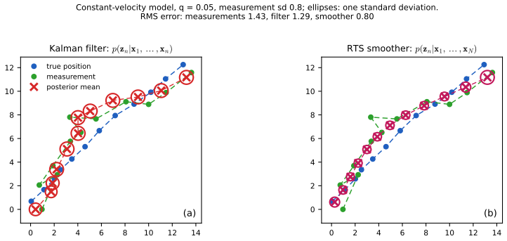
fig13_22. Download: PDF · SVGSmoothing: the Rauch-Tung-Striebel equations
pp. 640–641 For learning, and for off-line estimation, we want \(p(\mathbf{z}_n\given\mathbf{X})\), which also uses future observations. As for the HMM, this needs a backward pass; in the LDS literature it is written for \(\gamma\) itself (the \(\alpha\)-\(\gamma\) form of Result 13.21) rather than for \(\widehat\beta\):
\[ \gamma(\mathbf{z}_n)=\widehat\alpha(\mathbf{z}_n)\widehat\beta(\mathbf{z}_n)=\N(\mathbf{z}_n\given\widehat{\bm\mu}_n,\widehat{\mathbf{V}}_n). \tag{13.98} \]The starting point is the scaled backward recursion (13.62), for densities:
\[ c_{n+1}\widehat\beta(\mathbf{z}_n)=\int\widehat\beta(\mathbf{z}_{n+1})\,p(\mathbf{x}_{n+1}\given\mathbf{z}_{n+1})\,p(\mathbf{z}_{n+1}\given\mathbf{z}_n)\,\d\mathbf{z}_{n+1}. \tag{13.99} \]Result 13.33 (the RTS smoother; Exercise 13.29) p. 641, (13.100)–(13.102)
Starting from \(\widehat{\bm\mu}_N=\bm\mu_N\), \(\widehat{\mathbf{V}}_N=\mathbf{V}_N\) and going backwards,
\[ \widehat{\bm\mu}_n=\bm\mu_n+\mathbf{J}_n\big(\widehat{\bm\mu}_{n+1}-\mathbf{A}\bm\mu_n\big) \tag{13.100} \] \[ \widehat{\mathbf{V}}_n=\mathbf{V}_n+\mathbf{J}_n\big(\widehat{\mathbf{V}}_{n+1}-\mathbf{P}_n\big)\mathbf{J}_n^\T \tag{13.101} \] \[ \mathbf{J}_n=\mathbf{V}_n\mathbf{A}^\T(\mathbf{P}_n)^{-1}, \tag{13.102} \]where \(\mathbf{P}_n\)
Derivation
Step 1: turn (13.99) into a recursion for \(\gamma\). Multiply both sides of (13.99) by \(\widehat\alpha(\mathbf{z}_n)\). On the left, \(c_{n+1}\widehat\alpha(\mathbf{z}_n)\widehat\beta(\mathbf{z}_n)\)
The fraction is \(p(\mathbf{z}_n\given\mathbf{z}_{n+1},\mathbf{x}_{1:n})\) by Bayes' theorem (the numerator is \(p(\mathbf{z}_n\given\mathbf{x}_{1:n})p(\mathbf{z}_{n+1}\given\mathbf{z}_n)\)
Step 2: the backward conditional. \(p(\mathbf{z}_n\given\mathbf{z}_{n+1},\mathbf{x}_{1:n})\)
The covariance step is Woodbury (C.7) with \(\mathbf{P}_n\)
Step 3: integrate against \(\gamma(\mathbf{z}_{n+1})\). If \(\mathbf{z}_{n+1}\)
which are (13.100) and (13.101). (This is Result T.15's marginal once more.) At \(n=N\), \(\gamma(\mathbf{z}_N)\)
The identity \(\mathbf{A}\mathbf{V}_n\)
Algorithm 13.5 (Kalman smoother, RTS form) p. 641
- Run the Kalman filter (Algorithm 13.4), storing \(\bm\mu_n\), \(\mathbf{V}_n\) and \(\mathbf{P}_n\)
\({}=\mathbf{A}\mathbf{V}_n\mathbf{A}^\T+\bm\Gamma\). - Set \(\widehat{\bm\mu}_N=\bm\mu_N\), \(\widehat{\mathbf{V}}_N=\mathbf{V}_N\).
- For \(n=N-1,\dots,1\): \(\mathbf{J}_n\)
\({}=\mathbf{V}_n\mathbf{A}^\T\mathbf{P}_n^{-1}\), then (13.100) and (13.101). - For EM, also store \(\mathbf{J}_n\), which gives the pairwise covariances (13.104).
Result 13.34 (the pairwise posterior; Exercises 13.30 and 13.31) p. 641, (13.103)–(13.104)
From (13.65), for the LDS,
\[ \xi(\mathbf{z}_{n-1},\mathbf{z}_n)=(c_n)^{-1}\widehat\alpha(\mathbf{z}_{n-1})\,p(\mathbf{x}_n\given\mathbf{z}_n)\,p(\mathbf{z}_n\given\mathbf{z}_{n-1})\,\widehat\beta(\mathbf{z}_n)=\frac{\N(\mathbf{z}_{n-1}\given\bm\mu_{n-1},\mathbf{V}_{n-1})\,\N(\mathbf{z}_n\given\mathbf{A}\mathbf{z}_{n-1},\bm\Gamma)\,\N(\mathbf{x}_n\given\mathbf{C}\mathbf{z}_n,\bm\Sigma)\,\N(\mathbf{z}_n\given\widehat{\bm\mu}_n,\widehat{\mathbf{V}}_n)}{c_n\,\widehat\alpha(\mathbf{z}_n)}. \tag{13.103} \]It is a Gaussian over \((\mathbf{z}_{n-1},\mathbf{z}_n)\) with mean \((\widehat{\bm\mu}_{n-1},\widehat{\bm\mu}_n)\), marginal covariances \(\widehat{\mathbf{V}}_{n-1}\), \(\widehat{\mathbf{V}}_n\), and cross-covariance
\[ \cov[\mathbf{z}_{n-1},\mathbf{z}_n]=\mathbf{J}_{n-1}\widehat{\mathbf{V}}_n , \tag{13.104} \]with the convention \(\cov[\mathbf{a},\mathbf{b}]\)
Derivation
(13.103) (Exercise 13.30). The first expression is (13.65), valid for densities. Substitute (13.84) at \(n-1\), (13.75), (13.76), and \(\widehat\beta(\mathbf{z}_n)\)
Simplify (Exercise 13.31). By (13.85)–(13.87), \(c_n\widehat\alpha(\mathbf{z}_n)\)
the backward conditional of Step 2 of Result 13.33 (with \(n-1\) in place of \(n\)) times the smoothed marginal of \(\mathbf{z}_n\). So \(\mathbf{z}_{n-1}\)
(Checked numerically against the cross-covariance block of the full joint Gaussian.) ∎
13.3.2 Learning in LDS
pp. 642–644 The parameters \(\bm\theta\)
(expectations under \(p(\mathbf{Z}\given\mathbf{X},\bm\theta^{\rm old})\)). These follow from \(\E[\mathbf{a}\mathbf{b}^\T]\)
The complete-data log likelihood is the log of (13.6),
\[ \ln p(\mathbf{X},\mathbf{Z}\given\bm\theta)=\ln p(\mathbf{z}_1\given\bm\mu_0,\mathbf{P}_0)+\sum_{n=2}^{N}\ln p(\mathbf{z}_n\given\mathbf{z}_{n-1},\mathbf{A},\bm\Gamma)+\sum_{n=1}^{N}\ln p(\mathbf{x}_n\given\mathbf{z}_n,\mathbf{C},\bm\Sigma), \tag{13.108} \] \[ Q(\bm\theta,\bm\theta^{\rm old})=\E_{\mathbf{Z}\given\bm\theta^{\rm old}}\big[\ln p(\mathbf{X},\mathbf{Z}\given\bm\theta)\big]. \tag{13.109} \]The three groups of parameters appear in separate terms, so they are maximised separately. One tool is used throughout: for vectors \(\mathbf{a},\mathbf{b}\) and a matrix \(\mathbf{M}\), \(\E[\mathbf{a}^\T\mathbf{M}\mathbf{b}]\)
Result 13.35 (M step for the initial state; Exercise 13.32) pp. 642–643, (13.110)–(13.111)
\[ \bm\mu_0^{\rm new}=\E[\mathbf{z}_1] \tag{13.110} \] \[ \mathbf{P}_0^{\rm new}=\E[\mathbf{z}_1\mathbf{z}_1^\T]-\E[\mathbf{z}_1]\E[\mathbf{z}_1^\T]. \tag{13.111} \]That is, \(\bm\mu_0^{\rm new}=\widehat{\bm\mu}_1\) and \(\mathbf{P}_0^{\rm new}=\widehat{\mathbf{V}}_1\).
Derivation
The terms of \(Q\) containing \(\bm\mu_0,\mathbf{P}_0\) are
\[ Q_0=-\tfrac12\ln|\mathbf{P}_0|-\tfrac12\E\big[(\mathbf{z}_1-\bm\mu_0)^\T\mathbf{P}_0^{-1}(\mathbf{z}_1-\bm\mu_0)\big]=-\tfrac12\ln|\mathbf{P}_0|-\tfrac12\Tr\big(\mathbf{P}_0^{-1}\mathbf{R}_0\big), \]with \(\mathbf{R}_0\)
Result 13.36 (M step for the dynamics; Exercise 13.33) p. 643, (13.112)–(13.114)
The relevant part of \(Q\) is
\[ Q(\bm\theta,\bm\theta^{\rm old})=-\frac{N-1}{2}\ln|\bm\Gamma|-\E_{\mathbf{Z}\given\bm\theta^{\rm old}}\left[\frac12\sum_{n=2}^{N}(\mathbf{z}_n-\mathbf{A}\mathbf{z}_{n-1})^\T\bm\Gamma^{-1}(\mathbf{z}_n-\mathbf{A}\mathbf{z}_{n-1})\right]+\const, \tag{13.112} \]maximised by
\[ \mathbf{A}^{\rm new}=\left(\sum_{n=2}^{N}\E\big[\mathbf{z}_n\mathbf{z}_{n-1}^\T\big]\right)\left(\sum_{n=2}^{N}\E\big[\mathbf{z}_{n-1}\mathbf{z}_{n-1}^\T\big]\right)^{-1} \tag{13.113} \] \[ \bm\Gamma^{\rm new}=\frac{1}{N-1}\sum_{n=2}^{N}\Big\{\E\big[\mathbf{z}_n\mathbf{z}_n^\T\big]-\mathbf{A}^{\rm new}\E\big[\mathbf{z}_{n-1}\mathbf{z}_n^\T\big]-\E\big[\mathbf{z}_n\mathbf{z}_{n-1}^\T\big](\mathbf{A}^{\rm new})^\T+\mathbf{A}^{\rm new}\E\big[\mathbf{z}_{n-1}\mathbf{z}_{n-1}^\T\big](\mathbf{A}^{\rm new})^\T\Big\}, \tag{13.114} \]which simplifies to \(\bm\Gamma^{\rm new}\)
Derivation
The objective. (13.112) is the log of (13.75) summed over \(n\ge2\): each term contributes \(-\frac12\ln|\bm\Gamma|\) and the quadratic form. By the trace trick, the expectation is \(\frac12\Tr(\bm\Gamma^{-1}\mathbf{R}(\mathbf{A}))\) with
\[ \mathbf{R}(\mathbf{A})=\sum_{n=2}^{N}\E\big[(\mathbf{z}_n-\mathbf{A}\mathbf{z}_{n-1})(\mathbf{z}_n-\mathbf{A}\mathbf{z}_{n-1})^\T\big]=\mathbf{S}_{11}-\mathbf{A}\mathbf{S}_{10}^\T-\mathbf{S}_{10}\mathbf{A}^\T+\mathbf{A}\mathbf{S}_{00}\mathbf{A}^\T, \]where \(\mathbf{S}_{11}\)
Maximise over \(\mathbf{A}\). Using \(\partial\Tr(\mathbf{X}\mathbf{A})/\partial\mathbf{A}\)
(For the cross terms: \(\Tr(\bm\Gamma^{-1}\mathbf{A}\mathbf{S}_{10}^\T)\)
Maximise over \(\bm\Gamma\). With \(\mathbf{A}=\mathbf{A}^{\rm new}\) and \(\bm\Lambda=\bm\Gamma^{-1}\), the objective is \(\frac{N-1}2\ln|\bm\Lambda|\)
Result 13.37 (M step for the emissions; Exercise 13.34) p. 643, (13.115)–(13.116)
The relevant part of \(Q\) is \(-\frac N2\ln|\bm\Sigma|\)
which simplifies to \(\bm\Sigma^{\rm new}\)
Derivation
Exactly as in Result 13.36, with \(\mathbf{z}_n\) in place of \(\mathbf{z}_{n-1}\), \(\mathbf{x}_n\) in place of \(\mathbf{z}_n\), and \(N\) terms. By the trace trick, the expectation is \(\frac12\Tr(\bm\Sigma^{-1}\mathbf{R}(\mathbf{C}))\) with \(\mathbf{R}(\mathbf{C})\)
Algorithm 13.6 (EM for the linear dynamical system) pp. 642–643
- E step. Kalman filter and RTS smoother at \(\bm\theta^{\rm old}\); moments (13.105)–(13.107); log likelihood \(\sum_n\ln c_n\).
- M step. \(\bm\mu_0,\mathbf{P}_0\) by (13.110)–(13.111); \(\mathbf{A}\) by (13.113), then \(\bm\Gamma\) by (13.114); \(\mathbf{C}\) by (13.115), then \(\bm\Sigma\) by (13.116).
- Repeat until the log likelihood stops increasing.
Remarks. (i) The likelihood is invariant under \(\mathbf{z}\mapsto\mathbf{G}\mathbf{z}\) for invertible \(\mathbf{G}\) (with \(\mathbf{A}\mapsto\mathbf{G}\mathbf{A}\mathbf{G}^{-1}\), \(\mathbf{C}\mapsto\mathbf{C}\mathbf{G}^{-1}\), \(\bm\Gamma\mapsto\mathbf{G}\bm\Gamma\mathbf{G}^\T\), \(\bm\mu_0\mapsto\mathbf{G}\bm\mu_0\), \(\mathbf{P}_0\mapsto\mathbf{G}\mathbf{P}_0\mathbf{G}^\T\)), so the parameters are identifiable only up to such a change of basis, as for factor analysis; one often fixes \(\bm\Gamma=\mathbf{I}\) or \(\mathbf{C}\) partly. (ii) With one sequence, \(\mathbf{P}_0^{\rm new}=\widehat{\mathbf{V}}_1\) is estimated from a single state and tends to shrink; with \(R\) sequences the M steps sum over sequences, as in Exercise 13.12. (iii) Priors give MAP estimates directly, and a variational Bayesian treatment is possible with the methods of Chapter 10.
13.3.3 Extensions of LDS
p. 644 A linear-Gaussian model gives efficient algorithms but also a Gaussian marginal distribution for the observations, which is often too restrictive. The book sketches three ways out.
Filling the gap 13.2: Gaussian-mixture initial state is fine, Gaussian-mixture emissions are not p. 644, (13.85)
The book states that a \(K\)-component mixture for \(p(\mathbf{z}_1)\) keeps every \(\widehat\alpha(\mathbf{z}_n)\) a \(K\)-component mixture, while a \(K\)-component mixture emission makes \(\widehat\alpha(\mathbf{z}_n)\) a mixture of \(K^n\) Gaussians. Here is why.
Derivation
Mixture initial state. Let \(\widehat\alpha(\mathbf{z}_{n-1})\)
Mixture emission. Let \(p(\mathbf{x}_n\given\mathbf{z}_n)\)
Approximate filtering. Departures from the linear-Gaussian form make inference intractable. One can keep a Gaussian approximation of \(\widehat\alpha\) by moment matching at each step (assumed density filtering, or its iterated form, expectation propagation, Section 10.7), use sampling (Section 13.3.4), or linearise the model, which gives the extended Kalman filter.
Algorithm 13.7 (the extended Kalman filter) p. 644
Model: \(\mathbf{z}_n\)
- Predict: \(\mathbf{m}_n=\mathbf{f}(\bm\mu_{n-1})\), \(\mathbf{F}_n\)
\({}=\partial\mathbf{f}/\partial\mathbf{z}\big|_{\bm\mu_{n-1}}\), \(\mathbf{P}_{n-1}\) \({}=\mathbf{F}_n\mathbf{V}_{n-1}\mathbf{F}_n^\T\) \({}+\bm\Gamma\). - Update: \(\mathbf{H}_n\)
\({}=\partial\mathbf{h}/\partial\mathbf{z}\big|_{\mathbf{m}_n}\), \(\mathbf{S}_n\) \({}=\mathbf{H}_n\mathbf{P}_{n-1}\mathbf{H}_n^\T\) \({}+\bm\Sigma\), \(\mathbf{K}_n\) \({}=\mathbf{P}_{n-1}\mathbf{H}_n^\T\mathbf{S}_n^{-1}\), \(\bm\mu_n\) \({}=\mathbf{m}_n\) \({}+\mathbf{K}_n(\mathbf{x}_n-\mathbf{h}(\mathbf{m}_n))\), \(\mathbf{V}_n\) \({}=(\mathbf{I}-\mathbf{K}_n\mathbf{H}_n)\mathbf{P}_{n-1}\).
Derivation
Replace \(\mathbf{f}\) by its first-order Taylor expansion about the current mean, \(\mathbf{f}(\mathbf{z}_{n-1})\)
Switching state space models (Ghahramani and Hinton, 2000). Combine an HMM with several LDSs: \(M\) independent linear-Gaussian latent chains \(\mathbf{z}^{(1)},\dots,\mathbf{z}^{(M)}\) evolve in parallel, a discrete Markov chain \(s_n\in\{1,\dots,M\}\) acts as a switch, and \(\mathbf{x}_n\) is emitted from the chain selected by \(s_n\), \(p(\mathbf{x}_n\given s_n=m,\mathbf{z}_n^{(1:M)})\)
13.3.4 Particle filters
pp. 645–646 For state space models that are not linear-Gaussian (a non-Gaussian emission density, nonlinear dynamics), sampling gives a general inference method: the particle filter, or sequential Monte Carlo, which applies the sampling-importance-resampling idea of Section 11.1.5 at every time step. It has appeared as the bootstrap filter (Gordon et al., 1993), survival of the fittest (Kanazawa et al., 1995) and the condensation algorithm (Isard and Blake, 1998). Write \(\mathbf{X}_n=(\mathbf{x}_1,\dots,\mathbf{x}_n)\). The graph of Figure 13.5 gives
\[ p(\mathbf{z}_{n+1}\given\mathbf{z}_n,\mathbf{X}_n)=p(\mathbf{z}_{n+1}\given\mathbf{z}_n) \tag{13.120} \] \[ p(\mathbf{x}_n\given\mathbf{z}_n,\mathbf{X}_{n-1})=p(\mathbf{x}_n\given\mathbf{z}_n) \tag{13.121} \](both are instances of Result 13.11: (13.120) is (13.31) with \(N=n\), and (13.121) is (13.25)).
Result 13.38 (one step of the particle filter as importance sampling) pp. 645–646, (13.117)–(13.119)
(a) If \(\mathbf{z}_n^{(1)},\dots,\mathbf{z}_n^{(L)}\) are drawn from the predictive distribution \(p(\mathbf{z}_n\given\mathbf{X}_{n-1})\), then for any \(f\)
\[ \E[f(\mathbf{z}_n)\given\mathbf{X}_n]=\frac{\int f(\mathbf{z}_n)\,p(\mathbf{x}_n\given\mathbf{z}_n)\,p(\mathbf{z}_n\given\mathbf{X}_{n-1})\,\d\mathbf{z}_n}{\int p(\mathbf{x}_n\given\mathbf{z}_n)\,p(\mathbf{z}_n\given\mathbf{X}_{n-1})\,\d\mathbf{z}_n}\simeq\sum_{l=1}^{L}w_n^{(l)}f(\mathbf{z}_n^{(l)}), \tag{13.117} \] \[ w_n^{(l)}=\frac{p(\mathbf{x}_n\given\mathbf{z}_n^{(l)})}{\sum_{m=1}^{L}p(\mathbf{x}_n\given\mathbf{z}_n^{(m)})}, \tag{13.118} \]with \(0\le w_n^{(l)}\le1\), \(\sum_lw_n^{(l)}=1\). The weighted particles represent the filtered distribution \(p(\mathbf{z}_n\given\mathbf{X}_n)\), and the estimate is consistent as \(L\to\infty\).
(b) The next predictive distribution is then approximately a mixture:
\[ p(\mathbf{z}_{n+1}\given\mathbf{X}_n)=\frac{\int p(\mathbf{z}_{n+1}\given\mathbf{z}_n)\,p(\mathbf{x}_n\given\mathbf{z}_n)\,p(\mathbf{z}_n\given\mathbf{X}_{n-1})\,\d\mathbf{z}_n}{\int p(\mathbf{x}_n\given\mathbf{z}_n)\,p(\mathbf{z}_n\given\mathbf{X}_{n-1})\,\d\mathbf{z}_n}\simeq\sum_{l}w_n^{(l)}\,p(\mathbf{z}_{n+1}\given\mathbf{z}_n^{(l)}), \tag{13.119} \]which is sampled by picking a component \(l\) with probability \(w_n^{(l)}\) and drawing from \(p(\mathbf{z}_{n+1}\given\mathbf{z}_n^{(l)})\). Errata. In some printings the text after (13.118) has \(p(\mathbf{z}_n\given\mathbf{x}_n)\) for \(p(\mathbf{z}_n\given\mathbf{X}_n)\), and the last relation of (13.119) is printed as "\(=\)"; it is an approximation, "\(\simeq\)".
Derivation
(13.117). By Bayes' theorem with \(\mathbf{X}_{n-1}\) as background, \(p(\mathbf{z}_n\given\mathbf{X}_n)\)
(13.119). By the sum rule and (13.120), \(p(\mathbf{z}_{n+1}\given\mathbf{X}_n)\)
Algorithm 13.8 (bootstrap particle filter: sequential importance resampling) p. 646
- Draw \(\mathbf{z}_1^{(l)}\sim p(\mathbf{z}_1)\), \(l=1,\dots,L\).
- For \(n=1,2,\dots\):
- Weight: \(\tilde w^{(l)}\)
\({}=p(\mathbf{x}_n\given\mathbf{z}_n^{(l)})\), \(w_n^{(l)}=\tilde w^{(l)}/\sum_m\tilde w^{(m)}\) (13.118). Estimates of \(\E[f(\mathbf{z}_n)\given\mathbf{X}_n]\) use (13.117). The average \(\frac1L\sum_l\tilde w^{(l)}\) estimates \(c_n=p(\mathbf{x}_n\given\mathbf{X}_{n-1})\), and the product of these estimates estimates \(p(\mathbf{X}_n)\). - Resample: draw indices \(a^{(1)},\dots,a^{(L)}\) with \(\Pr(a=l)=w_n^{(l)}\).
- Propagate: \(\mathbf{z}_{n+1}^{(l)}\)
\({}\sim p(\mathbf{z}_{n+1}\given\mathbf{z}_n^{(a^{(l)})})\). Steps (b)–(c) sample the mixture (13.119).
- Weight: \(\tilde w^{(l)}\)
Work per step is \(O(L)\) density evaluations. In computations it is better to compute the weights from log-likelihoods with the maximum subtracted, to avoid underflow.
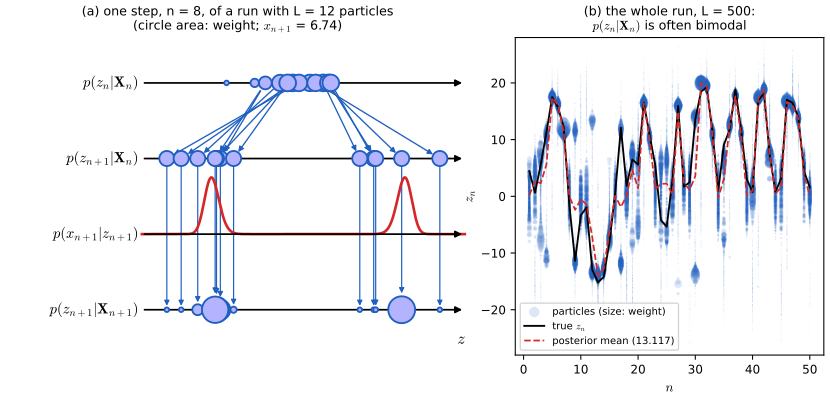
fig13_23. Download: PDF · SVGResult 13.39 (the weight recursion of sequential importance sampling)
Treat each particle as a whole trajectory \(\mathbf{z}_{1:n}^{(l)}\) with weight \(w_{n-1}^{(l)}\) targeting \(p(\mathbf{z}_{1:n-1}\given\mathbf{X}_{n-1})\). Extend each by \(\mathbf{z}_n^{(l)}\)
are a weighted sample for \(p(\mathbf{z}_{1:n}\given\mathbf{X}_n)\). With the bootstrap proposal \(q=p(\mathbf{z}_n\given\mathbf{z}_{n-1})\), \(w_n\)
Derivation
Target recursion. From (13.6) for \(n\) steps and the definition of conditional probability,
\[ p(\mathbf{z}_{1:n}\given\mathbf{X}_n)=\frac{p(\mathbf{z}_{1:n},\mathbf{X}_n)}{p(\mathbf{X}_n)}=\frac{p(\mathbf{z}_{1:n-1},\mathbf{X}_{n-1})\,p(\mathbf{z}_n\given\mathbf{z}_{n-1})\,p(\mathbf{x}_n\given\mathbf{z}_n)}{p(\mathbf{X}_{n-1})\,p(\mathbf{x}_n\given\mathbf{X}_{n-1})}=p(\mathbf{z}_{1:n-1}\given\mathbf{X}_{n-1})\,\frac{p(\mathbf{z}_n\given\mathbf{z}_{n-1})\,p(\mathbf{x}_n\given\mathbf{z}_n)}{p(\mathbf{x}_n\given\mathbf{X}_{n-1})}. \]Proposal for the trajectory. If the old trajectories have (unnormalised) importance weights \(w_{n-1}\)
which is the stated recursion, the last factor being a constant absorbed by the normalisation. Resampling replaces a weighted sample by an unweighted one with (approximately) the same distribution (Result 11.13), so after it every \(w_{n-1}^{(l)}=1/L\).
Optimal proposal. With \(q\)
Degeneracy and resampling. Without resampling, the weights of sequential importance sampling become more and more uneven as \(n\) grows (the variance of the product of weight factors increases), until one trajectory carries almost all the weight. The effective sample size \(L_{\rm eff}=1/\sum_l(w^{(l)})^2\) (Result 11.12) measures this; a common rule resamples only when \(L_{\rm eff}\lt L/2\). Resampling at every step, as in the book, fights degeneracy in the current state but impoverishes the past: after many steps all particles share a few common ancestors, so particle approximations of \(p(\mathbf{z}_{1:n}\given\mathbf{X}_n)\) for early times are poor, while the filtered marginal \(p(\mathbf{z}_n\given\mathbf{X}_n)\) stays accurate. Lower-variance resampling schemes (systematic, stratified) replace the independent multinomial draws. With too few particles, or very informative observations (a narrow likelihood), almost all particles get negligible weight in a single step and the filter can lose track.
For a quantitative version of the last demo: on a linear-Gaussian model, the root-mean-square difference between the bootstrap filter's posterior mean and the exact Kalman mean was 0.197, 0.055, 0.016 and 0.0056 for \(L=30\), 300, 3000 and 30000 particles in the course code, falling by about \(\sqrt{10}\) for each tenfold increase, as the \(L^{-1/2}\) rate predicts. Without resampling the effective sample size (\(L=500\)) fell to about 1.1; with resampling at every step it stayed near 169.
Exercises
All 34 exercises of Chapter 13 (Bishop, 2006, pp. 646–652), restated in my own words, with complete solutions (hidden). Stars give the book's difficulty and "www" marks the exercises with official solutions. Many exercises are the derivations of the results above; their solutions summarise the argument and link to the full version.
Exercise 13.1 (★, www). Use d-separation to show that the first-order chain of Figure 13.3 satisfies (13.3) for \(n=2,\dots,N\), and that the second-order chain of Figure 13.4 satisfies (13.122) for \(n=3,\dots,N\).
Solution
First order: every path from \(\mathbf{x}_m\), \(m\lt n-1\), to \(\mathbf{x}_n\) runs along the chain through \(\mathbf{x}_{n-1}\), where it is head-to-tail; \(\mathbf{x}_{n-1}\) is observed, so all such paths are blocked. Second order: a path entering \(\mathbf{x}_n\) through one of its parents \(\mathbf{x}_{n-1},\mathbf{x}_{n-2}\) is head-to-tail or tail-to-tail at that observed parent and is blocked; a path entering \(\mathbf{x}_n\) through a child is head-to-head at its latest node, all of whose descendants are later than \(n\) and unobserved, so it is blocked too. Details: Result 13.1, Result 13.2.
Exercise 13.2 (★★). Using only the sum and product rules, show that the joint (13.2) satisfies (13.3), and that (13.4) satisfies \(p(\mathbf{x}_n\given\mathbf{x}_{1:n-1})\)
\({}=p(\mathbf{x}_n\given\mathbf{x}_{n-1},\mathbf{x}_{n-2})\) (13.123). Solution
Summing (13.2) over \(\mathbf{x}_N,\mathbf{x}_{N-1},\dots,\mathbf{x}_{n+1}\) in this order removes one normalised factor at a time, so \(p(\mathbf{x}_{1:n})\)
\({}=p(\mathbf{x}_1)\prod_{m=2}^{n}p(\mathbf{x}_m\given\mathbf{x}_{m-1})\). Then \(p(\mathbf{x}_n\given\mathbf{x}_{1:n-1})\) \({}=p(\mathbf{x}_{1:n})/p(\mathbf{x}_{1:n-1})\) \({}=p(\mathbf{x}_n\given\mathbf{x}_{n-1})\). The same steps on (13.4) leave the single factor \(p(\mathbf{x}_n\given\mathbf{x}_{n-1},\mathbf{x}_{n-2})\). See Result 13.1 and Result 13.2, which also check that these factors are the true conditionals of the joint. Exercise 13.3 (★). Use d-separation to show that the observed variables of the state space model of Figure 13.5 satisfy no conditional independence property, and hence no Markov property of finite order.
Solution
For \(m\lt n\) and any set of other observed nodes, the path \(\mathbf{x}_m\leftarrow\mathbf{z}_m\)
\({}\to\cdots\) \({}\to\mathbf{z}_n\) \({}\to\mathbf{x}_n\) passes only through latent nodes, never observed, at which it is tail-to-tail or head-to-tail; it has no head-to-head node. So it is never blocked, and no conditional independence between observations follows from the graph. An explicit HMM in which the predictive distribution depends on every past observation is in Result 13.4. Exercise 13.4 (★★, www). The emission densities are a parametric model \(p(\mathbf{x}\given\mathbf{z},\mathbf{w})\), such as a linear regression or a neural network. How can \(\mathbf{w}\) be learned by maximum likelihood?
Solution
Use EM exactly as in Algorithm 13.1, with \(\mathbf{w}\) in place of \(\bm\phi\). The E step is unchanged (it only needs the numbers \(p(\mathbf{x}_n\given z_{nk}=1,\mathbf{w}^{\rm old})\)). In the M step only the last term of (13.17) involves \(\mathbf{w}\): maximise the weighted log likelihood \(\sum_n\sum_k\gamma(z_{nk})\ln p(\mathbf{x}_n\given z_{nk}=1,\mathbf{w})\).
Linear regression emissions (typically with an input \(\mathbf{u}_n\), as in the input-output HMM of Figure 13.18): if \(p(\mathbf{x}_n\given z_{nk}=1,\mathbf{w})\)
\({}=\N(\mathbf{x}_n\given\mathbf{W}_k\bm\phi(\mathbf{u}_n),\beta_k^{-1}\mathbf{I})\), each \(\mathbf{W}_k\) solves a weighted least-squares problem: with \(\bm\Phi\) the design matrix and \(\mathbf{R}_k\) \({}=\diag(\gamma(z_{1k}),\dots,\gamma(z_{Nk}))\), \(\mathbf{W}_k^\T\) \({}=(\bm\Phi^\T\mathbf{R}_k\bm\Phi)^{-1}\bm\Phi^\T\mathbf{R}_k\mathbf{X}\), and \(1/\beta_k\) is the weighted mean squared residual divided by \(D\). Neural network: there is no closed form; take a few gradient steps on the weighted log likelihood. Any increase of \(Q\) still increases the likelihood (generalised EM, Section 9.4). Alternatively, maximise \(\ln p(\mathbf{X}\given\mathbf{w})\) directly by gradient ascent, using Fisher's identity (Filling the gap 13.1): its gradient is \(\sum_n\sum_k\gamma(z_{nk})\nabla_{\mathbf{w}}\ln p(\mathbf{x}_n\given z_{nk}=1,\mathbf{w})\). Discriminative networks (p. 612): a network trained to output \(p(\mathbf{z}\given\mathbf{x})\) can be used because the recursions only need the emissions up to a factor that does not depend on \(\mathbf{z}_n\): by Bayes, \(p(\mathbf{x}_n\given\mathbf{z}_n)\)
\({}=p(\mathbf{z}_n\given\mathbf{x}_n)p(\mathbf{x}_n)/p(\mathbf{z}_n)\), and replacing \(e_{nk}\) by \(\kappa_ne_{nk}\) multiplies \(\alpha(\mathbf{z}_m)\) for \(m\ge n\) and \(p(\mathbf{X})\) by \(\kappa_n\) and leaves \(\gamma\) and \(\xi\) unchanged. So the "scaled likelihoods" \(p(\mathbf{z}_n\given\mathbf{x}_n)/p(\mathbf{z}_n)\) can be used in place of \(p(\mathbf{x}_n\given\mathbf{z}_n)\). Exercise 13.5 (★★). Derive the M-step equations (13.18) and (13.19) by maximising (13.17) with Lagrange multipliers.
Solution
For \(\bm\pi\): stationarity of \(\sum_k\gamma(z_{1k})\ln\pi_k\)
\({}+\lambda(\sum_k\pi_k-1)\) gives \(\pi_k=-\gamma(z_{1k})/\lambda\), and the constraint gives \(\lambda=-\sum_j\gamma(z_{1j})\). For row \(j\) of \(\mathbf{A}\): stationarity of \(\sum_k c_{jk}\ln A_{jk}\) \({}+\lambda_j(\sum_kA_{jk}-1)\), \(c_{jk}=\sum_{n\ge2}\xi(z_{n-1,j},z_{nk})\), gives \(A_{jk}=c_{jk}/\sum_lc_{jl}\). Both are global maxima (concave objectives on the simplex, or Gibbs' inequality). Full details: Result 13.7. Exercise 13.6 (★). Show that elements of \(\bm\pi\) or \(\mathbf{A}\) initialised to zero stay zero under EM.
Solution
\(\xi(z_{n-1,j},z_{nk})\) contains the factor \(A_{jk}\) by (13.43), and \(\gamma(z_{1k})\) contains \(\pi_k\) through \(\alpha(z_{1k})\)
\({}=\pi_kp(\mathbf{x}_1\given\bm\phi_k)\). If the old value is zero, all these numbers vanish, and so do the numerators of (13.18)–(13.19). Induction over iterations. See Result 13.10. Exercise 13.7 (★). For Gaussian emissions, show that maximising \(Q\) over the means and covariances gives (13.20) and (13.21).
Solution
Only \(\sum_n\gamma(z_{nk})\ln\N(\mathbf{x}_n\given\bm\mu_k,\bm\Sigma_k)\) depends on \(\bm\mu_k,\bm\Sigma_k\). Its gradient in \(\bm\mu_k\) is \(\bm\Sigma_k^{-1}\sum_n\gamma(z_{nk})(\mathbf{x}_n-\bm\mu_k)\), zero at (13.20). In terms of \(\bm\Lambda=\bm\Sigma_k^{-1}\) it is \(\frac{N_k}2\ln|\bm\Lambda|\)
\({}-\frac12\Tr(\bm\Lambda\mathbf{S}_k)\), maximised at \(\bm\Lambda^{-1}=\mathbf{S}_k/N_k\): (13.21). See Result 13.8. Exercise 13.8 (★★, www). For discrete (multinomial) observations show (13.22) and the M step (13.23); do the same for several binary (Bernoulli) outputs.
Solution
With 1-of-\(D\) coding, (13.22) picks out \(\mu_{ik}\) when \(x_i=z_k=1\). The emission part of \(Q\) is \(\sum_k\sum_i c_{ik}\ln\mu_{ik}\) with \(c_{ik}=\sum_n\gamma(z_{nk})x_{ni}\); a Lagrange multiplier per state gives \(\mu_{ik}=c_{ik}/\sum_{i'}c_{i'k}\), and \(\sum_{i'}x_{ni'}=1\) turns the denominator into \(\sum_n\gamma(z_{nk})\): (13.23). For independent binary outputs, \(p(\mathbf{x}\given\mathbf{z})\)
\({}=\prod_i\prod_k[\mu_{ik}^{x_i}(1-\mu_{ik})^{1-x_i}]^{z_k}\), each \(\mu_{ik}\) maximises \(\sum_n\gamma(z_{nk})\{x_{ni}\ln\mu_{ik}\) \({}+(1-x_{ni})\ln(1-\mu_{ik})\}\) without constraint, and the stationary point is again (13.23). See Result 13.9. Exercise 13.9 (★★, www). Verify (13.24)–(13.31) by d-separation.
Solution
In each case the conditioning set contains a latent node through which every connecting path passes head-to-tail or tail-to-tail: \(\mathbf{z}_n\) for (13.24), (13.25) and (13.29) (together with \(\mathbf{z}_{n-1}\)); \(\mathbf{z}_{n-1}\) for (13.26); \(\mathbf{z}_{n+1}\) for (13.27) and (13.28); \(\mathbf{z}_{N+1}\) for (13.30); \(\mathbf{z}_N\) for (13.31). Since the \(\mathbf{x}\)'s are leaves, no path has a head-to-head node except at an \(\mathbf{x}\), which cannot be an intermediate node of a path between the variables involved. The node-by-node check is in Result 13.12.
Exercise 13.10 (★★★). Verify (13.24)–(13.31) using only the sum and product rules applied to (13.6).
Solution
Group the factors of (13.6) into those involving times before \(n\) and \(\mathbf{z}_n\), the emission \(p(\mathbf{x}_n\given\mathbf{z}_n)\), and those after \(n\). The first group is \(p(\mathcal{P}_n,\mathbf{z}_n)\) and the last sums to one over the future, so given \(\mathbf{z}_n\) the past, \(\mathbf{x}_n\) and the future are mutually independent (Result 13.11). Each of the eight properties is this statement at a suitable time (\(n-1\), \(n\), \(n+1\), or in the chain extended to \(N+1\)), followed by summing out unwanted variables or moving variables into the conditioning set; the eight cases are worked out in Result 13.12.
Exercise 13.11 (★★). From (8.72), the marginal over the variables of a factor, and the messages of Section 13.2.3, derive (13.43).
Solution
(8.72) applied to \(f_n\) gives \(p(\mathbf{z}_{n-1},\mathbf{z}_n,\mathbf{X})\)
\({}=f_n(\mathbf{z}_{n-1},\mathbf{z}_n)\mu_{\mathbf{z}_{n-1}\to f_n}(\mathbf{z}_{n-1})\mu_{\mathbf{z}_n\to f_n}(\mathbf{z}_n)\). The variable nodes pass messages on unchanged, so the two messages are \(\mu_{f_{n-1}\to\mathbf{z}_{n-1}}\) \({}=\alpha(\mathbf{z}_{n-1})\) and \(\mu_{f_{n+1}\to\mathbf{z}_n}=\beta(\mathbf{z}_n)\); with \(f_n\) \({}=p(\mathbf{z}_n\given\mathbf{z}_{n-1})p(\mathbf{x}_n\given\mathbf{z}_n)\) and division by \(p(\mathbf{X})\) this is (13.43). See Result 13.18. Exercise 13.12 (★★). With \(R\) independent training sequences \(\mathbf{X}^{(r)}\), show that the E step runs forward-backward on each sequence separately and the M step becomes
\[ \pi_k=\frac{\sum_{r=1}^{R}\gamma(z_{1k}^{(r)})}{\sum_{r=1}^{R}\sum_{j=1}^{K}\gamma(z_{1j}^{(r)})},\qquad A_{jk}=\frac{\sum_{r=1}^{R}\sum_{n=2}^{N}\xi(z_{n-1,j}^{(r)},z_{n,k}^{(r)})}{\sum_{r=1}^{R}\sum_{l=1}^{K}\sum_{n=2}^{N}\xi(z_{n-1,j}^{(r)},z_{n,l}^{(r)})},\qquad \bm\mu_k=\frac{\sum_{r=1}^{R}\sum_{n=1}^{N}\gamma(z_{nk}^{(r)})\mathbf{x}_n^{(r)}}{\sum_{r=1}^{R}\sum_{n=1}^{N}\gamma(z_{nk}^{(r)})}. \tag{13.124–13.126} \]Solution
E step. Independent sequences with shared parameters have joint \(\prod_rp(\mathbf{X}^{(r)},\mathbf{Z}^{(r)}\given\bm\theta)\), so the posterior factorises, \(p(\mathbf{Z}^{(1:R)}\given\mathbf{X}^{(1:R)})\)
\({}=\prod_rp(\mathbf{Z}^{(r)}\given\mathbf{X}^{(r)})\): the marginals \(\gamma^{(r)}\), \(\xi^{(r)}\) of sequence \(r\) depend only on \(\mathbf{X}^{(r)}\) and are computed by running the \(\alpha\) and \(\beta\) recursions on that sequence alone. The log likelihood is \(\sum_r\ln p(\mathbf{X}^{(r)})\). M step. The complete-data log likelihood is a sum over \(r\) of terms of the form used in Result 13.6, so
\[ Q=\sum_k\Big(\sum_r\gamma(z_{1k}^{(r)})\Big)\ln\pi_k+\sum_{j,k}\Big(\sum_r\sum_{n\ge2}\xi(z_{n-1,j}^{(r)},z_{nk}^{(r)})\Big)\ln A_{jk}+\sum_r\sum_n\sum_k\gamma(z_{nk}^{(r)})\ln p(\mathbf{x}_n^{(r)}\given\bm\phi_k). \]This has exactly the form of (13.17) with the expected counts summed over sequences, so the Lagrange-multiplier argument of Result 13.7 gives (13.124)–(13.125) and the weighted Gaussian fit of Result 13.8 gives (13.126) (and the covariance analogously). For sequences of different lengths \(N_r\), the sums over \(n\) run to \(N_r\). (With one sequence, \(\pi\) is fitted to a single \(\mathbf{z}_1\); with \(R\) sequences, (13.124) averages \(R\) posterior distributions of the first state.)
Exercise 13.13 (★★, www). Using the definition (8.64) of factor-to-variable messages and (13.6), show that the message (13.50) equals \(\alpha(\mathbf{z}_n)\) of (13.34).
Solution
By (8.64), \(\mu_{f_n\to\mathbf{z}_n}(\mathbf{z}_n)\) is the sum over \(\mathbf{z}_1,\dots,\mathbf{z}_{n-1}\) of the product of all factors on the \(f_n\) side of \(\mathbf{z}_n\): \(h(\mathbf{z}_1)\prod_{m=2}^{n}f_m(\mathbf{z}_{m-1},\mathbf{z}_m)\)
\({}=p(\mathbf{z}_1)\prod_{m=2}^{n}p(\mathbf{z}_m\given\mathbf{z}_{m-1})\) \(\prod_{m=1}^{n}p(\mathbf{x}_m\given\mathbf{z}_m)\) \({}=p(\mathbf{x}_{1:n},\mathbf{z}_{1:n})\). Summing over \(\mathbf{z}_{1:n-1}\) gives \(p(\mathbf{x}_{1:n},\mathbf{z}_n)\) \({}=\alpha(\mathbf{z}_n)\). See Result 13.18. Exercise 13.14 (★★). Similarly, using (8.67), show that the message (13.52) equals \(\beta(\mathbf{z}_n)\) of (13.35).
Solution
The message \(\mu_{f_{n+1}\to\mathbf{z}_n}(\mathbf{z}_n)\) sums, over \(\mathbf{z}_{n+1},\dots,\mathbf{z}_N\), the product of the factors on the far side: \(\prod_{m=n+1}^{N}p(\mathbf{z}_m\given\mathbf{z}_{m-1})p(\mathbf{x}_m\given\mathbf{z}_m)\)
\({}=p(\mathbf{x}_{n+1:N},\mathbf{z}_{n+1:N}\given\mathbf{z}_n)\) (Result 13.11). The sum is \(p(\mathbf{x}_{n+1:N}\given\mathbf{z}_n)\) \({}=\beta(\mathbf{z}_n)\). See Result 13.18. Exercise 13.15 (★★). From (13.33) and (13.43), derive the scaled forms (13.64) and (13.65).
Solution
Substitute \(\alpha(\mathbf{z}_n)\)
\({}=(\prod_{m\le n}c_m)\widehat\alpha(\mathbf{z}_n)\), \(\beta(\mathbf{z}_n)\) \({}=(\prod_{m\gt n}c_m)\widehat\beta(\mathbf{z}_n)\) and \(p(\mathbf{X})=\prod_{m\le N}c_m\). In (13.33) all \(c\)'s cancel: \(\gamma=\widehat\alpha\widehat\beta\). In (13.43), \(\alpha(\mathbf{z}_{n-1})\beta(\mathbf{z}_n)\) carries every \(c_m\) except \(c_n\), so one \(c_n\) remains in the denominator: (13.65). See Result 13.20. Exercise 13.16 (★★★). Derive the Viterbi recursion (13.68), with \(\omega\) defined by (13.70) and initial condition (13.69), directly from (13.6), by taking logarithms and exchanging maximisations and sums.
Solution
\(\ln p(\mathbf{x}_{1:n},\mathbf{z}_{1:n})\)
\({}=\ln p(\mathbf{x}_{1:n-1},\mathbf{z}_{1:n-1})\) \({}+\ln p(\mathbf{z}_n\given\mathbf{z}_{n-1})\) \({}+\ln p(\mathbf{x}_n\given\mathbf{z}_n)\). Maximise over \(\mathbf{z}_{1:n-2}\) first: only the first term depends on them, and its maximum is \(\omega(\mathbf{z}_{n-1})\). Then maximise over \(\mathbf{z}_{n-1}\); the emission term does not depend on it and comes outside: \(\omega(\mathbf{z}_n)\) \({}=\ln p(\mathbf{x}_n\given\mathbf{z}_n)\) \({}+\max_{\mathbf{z}_{n-1}}\{\ln p(\mathbf{z}_n\given\mathbf{z}_{n-1})\) \({}+\omega(\mathbf{z}_{n-1})\}\). For \(n=1\), \(\omega(\mathbf{z}_1)\) \({}=\ln p(\mathbf{z}_1)\) \({}+\ln p(\mathbf{x}_1\given\mathbf{z}_1)\). See Result 13.22, and the back-tracking argument after Algorithm 13.3. Exercise 13.17 (★, www). Show that the input-output HMM of Figure 13.18 can be written as a chain factor graph like Figure 13.15, and give \(h(\mathbf{z}_1)\) and \(f_n(\mathbf{z}_{n-1},\mathbf{z}_n)\).
Solution
With the inputs and outputs observed, absorb each emission into the transition factor of the same time step: \(h(\mathbf{z}_1)\)
\({}=p(\mathbf{z}_1\given\mathbf{u}_1)\,p(\mathbf{x}_1\given\mathbf{z}_1,\mathbf{u}_1)\) and \(f_n(\mathbf{z}_{n-1},\mathbf{z}_n)\) \({}=p(\mathbf{z}_n\given\mathbf{z}_{n-1},\mathbf{u}_n)\,p(\mathbf{x}_n\given\mathbf{z}_n,\mathbf{u}_n)\) for \(2\le n\le N\). Their product is \(p(\mathbf{X},\mathbf{Z}\given\mathbf{U})\), and each factor involves at most two successive latent variables, so the graph is a chain (a tree). See Result 13.25. Exercise 13.18 (★★★). Using Exercise 13.17, derive the forward-backward recursions, with initial conditions, for the input-output HMM.
Solution
Sum-product on the chain of Exercise 13.17 gives, with \(A^{(n)}_{jk}\)
\[ \alpha(z_{1k})=p(z_{1k}=1\given\mathbf{u}_1)\,e_{1k},\qquad \alpha(z_{nk})=e_{nk}\sum_j\alpha(z_{n-1,j})A^{(n)}_{jk}, \] \[ \beta(z_{Nk})=1,\qquad \beta(z_{nj})=\sum_kA^{(n+1)}_{jk}\,e_{n+1,k}\,\beta(z_{n+1,k}), \]\({}=p(z_{nk}=1\given z_{n-1,j}=1,\mathbf{u}_n)\) and \(e_{nk}\) \({}=p(\mathbf{x}_n\given z_{nk}=1,\mathbf{u}_n)\): with \(\alpha(\mathbf{z}_n)\)
\({}=p(\mathbf{x}_{1:n},\mathbf{z}_n\given\mathbf{U})\), \(\beta(\mathbf{z}_n)\) \({}=p(\mathbf{x}_{n+1:N}\given\mathbf{z}_n,\mathbf{U})\), \(p(\mathbf{X}\given\mathbf{U})\) \({}=\sum_k\alpha(z_{Nk})\), \(\gamma=\alpha\beta/p(\mathbf{X}\given\mathbf{U})\) and \(\xi(z_{n-1,j},z_{nk})\) \({}=\alpha(z_{n-1,j})A^{(n)}_{jk}e_{nk}\beta(z_{nk})/p(\mathbf{X}\given\mathbf{U})\). The scaled version follows as in Section 13.2.4. In the M step the transition and emission models are now conditional models of \(\mathbf{z}_n\) and \(\mathbf{x}_n\) given \(\mathbf{u}_n\) (e.g. softmax regressions), fitted by maximising \(\sum_n\sum_{j,k}\xi\ln A^{(n)}_{jk}\) and \(\sum_n\sum_k\gamma\ln e_{nk}\), usually by a few gradient steps. Derivation: Result 13.25. Exercise 13.19 (★, www). Show that, for a linear dynamical system, maximising each posterior marginal \(p(\mathbf{z}_n\given\mathbf{X})\) separately gives the most probable latent sequence.
Solution
The joint posterior over \(\mathbf{Z}\) is Gaussian, so its mode is its mean; by (2.98) each marginal is Gaussian with the corresponding block of that mean, which is also its mode. Hence marginal modes and the joint mode coincide. See Result 13.28.
Exercise 13.20 (★★, www). Use (2.115) to prove (13.87).
Solution
In (2.113)–(2.115) put \(\mathbf{x}\to\mathbf{z}_{n-1}\), \(\bm\mu\to\bm\mu_{n-1}\), \(\bm\Lambda^{-1}\to\mathbf{V}_{n-1}\), \(\mathbf{y}\to\mathbf{z}_n\), \(\mathbf{A}\to\mathbf{A}\), \(\mathbf{b}\to\mathbf{0}\), \(\mathbf{L}^{-1}\to\bm\Gamma\). Then (2.115) reads \(\int\N(\mathbf{z}_n\given\mathbf{A}\mathbf{z}_{n-1},\bm\Gamma)\)
\(\N(\mathbf{z}_{n-1}\given\bm\mu_{n-1},\mathbf{V}_{n-1})\d\mathbf{z}_{n-1}\) \({}=\N(\mathbf{z}_n\given\mathbf{A}\bm\mu_{n-1},\bm\Gamma+\mathbf{A}\mathbf{V}_{n-1}\mathbf{A}^\T)\), which is (13.87)–(13.88). See Result 13.29. Exercise 13.21 (★★). Use (2.115), (2.116) and the identities (C.5) and (C.7) to derive (13.89)–(13.91) with the gain (13.92).
Solution
(2.116) with prior \(\N(\mathbf{z}_n\given\mathbf{A}\bm\mu_{n-1},\mathbf{P}_{n-1})\) and likelihood \(\N(\mathbf{x}_n\given\mathbf{C}\mathbf{z}_n,\bm\Sigma)\) gives \(\mathbf{V}_n\)
\({}=(\mathbf{P}_{n-1}^{-1}+\mathbf{C}^\T\bm\Sigma^{-1}\mathbf{C})^{-1}\) and \(\bm\mu_n\) \({}=\mathbf{V}_n(\mathbf{P}_{n-1}^{-1}\mathbf{A}\bm\mu_{n-1}+\mathbf{C}^\T\bm\Sigma^{-1}\mathbf{x}_n)\). (C.7) turns \(\mathbf{V}_n\) into \((\mathbf{I}-\mathbf{K}_n\mathbf{C})\mathbf{P}_{n-1}\); (C.5) gives \(\mathbf{V}_n\mathbf{C}^\T\bm\Sigma^{-1}\) \({}=\mathbf{K}_n\), and then \(\bm\mu_n\) \({}=(\mathbf{I}-\mathbf{K}_n\mathbf{C})\mathbf{A}\bm\mu_{n-1}\) \({}+\mathbf{K}_n\mathbf{x}_n\), which is (13.89). (2.115) gives the marginal of \(\mathbf{x}_n\), i.e. \(c_n\) in (13.91). Full derivation by completing the square: Result 13.30. Exercise 13.22 (★★, www). From (13.93), (13.76), (13.77) and (2.115), derive (13.96).
Solution
(13.93) says \(c_1\widehat\alpha(\mathbf{z}_1)\)
\({}=\N(\mathbf{z}_1\given\bm\mu_0,\mathbf{P}_0)\N(\mathbf{x}_1\given\mathbf{C}\mathbf{z}_1,\bm\Sigma)\). Integrating over \(\mathbf{z}_1\): the left gives \(c_1\) (as \(\widehat\alpha\) integrates to one), the right the marginal of \(\mathbf{x}_1\) in the linear-Gaussian model, which by (2.115) (with \(\mathbf{x}\to\mathbf{z}_1\), \(\bm\mu\to\bm\mu_0\), \(\bm\Lambda^{-1}\to\mathbf{P}_0\), \(\mathbf{A}\to\mathbf{C}\), \(\mathbf{b}\to\mathbf{0}\), \(\mathbf{L}^{-1}\to\bm\Sigma\)) is \(\N(\mathbf{x}_1\given\mathbf{C}\bm\mu_0,\bm\Sigma+\mathbf{C}\mathbf{P}_0\mathbf{C}^\T)\): (13.96). See Result 13.31. Exercise 13.23 (★★). From (13.93), (13.76), (13.77) and (2.116), derive (13.94), (13.95) and (13.97).
Solution
\(\widehat\alpha(\mathbf{z}_1)\)
\({}=p(\mathbf{z}_1\given\mathbf{x}_1)\), which (2.116) gives as \(\N(\mathbf{z}_1\given\mathbf{V}_1(\mathbf{C}^\T\bm\Sigma^{-1}\mathbf{x}_1+\mathbf{P}_0^{-1}\bm\mu_0),\mathbf{V}_1)\) with \(\mathbf{V}_1\) \({}=(\mathbf{P}_0^{-1}+\mathbf{C}^\T\bm\Sigma^{-1}\mathbf{C})^{-1}\). Exactly as in Exercise 13.21, (C.7) gives \(\mathbf{V}_1\) \({}=(\mathbf{I}-\mathbf{K}_1\mathbf{C})\mathbf{P}_0\) with \(\mathbf{K}_1\) of (13.97), and (C.5) gives \(\bm\mu_1\) \({}=\bm\mu_0\) \({}+\mathbf{K}_1(\mathbf{x}_1-\mathbf{C}\bm\mu_0)\). See Result 13.31. Exercise 13.24 (★★, www). Allow constant terms: \(p(\mathbf{z}_n\given\mathbf{z}_{n-1})\)
\({}=\N(\mathbf{z}_n\given\mathbf{A}\mathbf{z}_{n-1}+\mathbf{a},\bm\Gamma)\) (13.127) and \(p(\mathbf{x}_n\given\mathbf{z}_n)\) \({}=\N(\mathbf{x}_n\given\mathbf{C}\mathbf{z}_n+\mathbf{c},\bm\Sigma)\) (13.128). Show that this fits the framework of the chapter by adding a state component fixed at one. Solution
Let \(\mathbf{z}'_n=(\mathbf{z}_n,1)\in\R^{M+1}\) and
\[ \mathbf{A}'=\begin{pmatrix}\mathbf{A}&\mathbf{a}\\\mathbf{0}^\T&1\end{pmatrix},\quad \bm\Gamma'=\begin{pmatrix}\bm\Gamma&\mathbf{0}\\\mathbf{0}^\T&0\end{pmatrix},\quad \mathbf{C}'=\begin{pmatrix}\mathbf{C}&\mathbf{c}\end{pmatrix},\quad \bm\mu_0'=\begin{pmatrix}\bm\mu_0\\1\end{pmatrix},\quad \mathbf{P}_0'=\begin{pmatrix}\mathbf{P}_0&\mathbf{0}\\\mathbf{0}^\T&0\end{pmatrix}. \]Then \(\mathbf{A}'\mathbf{z}'_{n-1}\)
\({}=(\mathbf{A}\mathbf{z}_{n-1}+\mathbf{a},1)\), and the zero variance in the last coordinate of \(\bm\Gamma'\) and \(\mathbf{P}_0'\) keeps that coordinate equal to 1 for ever; \(\mathbf{C}'\mathbf{z}'_n\) \({}=\mathbf{C}\mathbf{z}_n+\mathbf{c}\). So (13.127)–(13.128) are the standard LDS (13.75)–(13.77) in the augmented state (with a degenerate Gaussian). The Kalman filter never inverts \(\bm\Gamma'\) or \(\mathbf{P}'\) (it inverts \(\mathbf{S}_n\), which contains \(\bm\Sigma\succ0\)), so it runs unchanged. The smoother inverts \(\mathbf{P}'_n\), which is singular in the last coordinate; since that coordinate is known exactly, use the inverse of the upper-left \(M\times M\) block padded with zeros (a generalised inverse), or equivalently run the recursions on \(\mathbf{z}_n\) with predicted mean \(\mathbf{A}\bm\mu_{n-1}+\mathbf{a}\) and innovation \(\mathbf{x}_n\) \({}-\mathbf{C}(\mathbf{A}\bm\mu_{n-1}+\mathbf{a})\) \({}-\mathbf{c}\). In EM, the last row of \(\mathbf{A}'\) is held fixed and \((\mathbf{A},\mathbf{a})\), \((\mathbf{C},\mathbf{c})\) are estimated jointly by the regressions (13.113), (13.115) on the augmented moments. Exercise 13.25 (★★). For independent observations of a scalar Gaussian with unknown mean, model the mean as a latent state with \(A=C=1\), \(\Gamma=0\), initial \(\mu_0,P_0=\sigma_0^2\) and \(\Sigma=\sigma^2\). Show that the Kalman filter reproduces (2.141)–(2.142).
Solution
With \(\Gamma=0\), \(P_{n-1}=V_{n-1}\) and \(K_n=V_{n-1}/(V_{n-1}+\sigma^2)\). Then \(1/V_n=1/V_{n-1}+1/\sigma^2\) and \(\mu_n/V_n=\mu_{n-1}/V_{n-1}+x_n/\sigma^2\), and from \(V_0=\sigma_0^2\) induction gives \(1/V_N=1/\sigma_0^2+N/\sigma^2\) (2.142) and \(\mu_N\)
\({}=\frac{\sigma^2}{N\sigma_0^2+\sigma^2}\mu_0\) \({}+\frac{N\sigma_0^2}{N\sigma_0^2+\sigma^2}\mu_{\rm ML}\) (2.141). See Result 13.32(c). (Errata: in the exercise, "\(\mathbf{V}_0\)" and "\(m_0\)" should read \(P_0\) and \(\mu_0\), and the sentence fragment on p. 651 should read "in which \(\mathbf{C}=1\), \(\mathbf{A}=1\) and \(\bm\Gamma=0\)".) Exercise 13.26 (★★★). Take \(\mathbf{A}=\mathbf{0}\), \(\bm\Gamma=\mathbf{I}\), \(\bm\Sigma=\sigma^2\mathbf{I}\), \(\mathbf{C}=\mathbf{W}\) (and \(\bm\mu_0=\mathbf{0}\), \(\mathbf{P}_0=\mathbf{I}\)). Using (C.7), show that the filtered posterior (13.89)–(13.90) is the probabilistic PCA posterior (12.42) with \(\bm\mu=\mathbf{0}\).
Solution
With \(\mathbf{A}=\mathbf{0}\) the prediction is \(\N(\mathbf{0},\bm\Gamma)\)
\[ \bm\mu_n=\mathbf{K}_n\mathbf{x}_n=\mathbf{M}^{-1}\mathbf{W}^\T\mathbf{x}_n,\qquad \mathbf{V}_n=\mathbf{I}-\mathbf{K}_n\mathbf{W}=\mathbf{I}-\mathbf{M}^{-1}\mathbf{W}^\T\mathbf{W}=\mathbf{M}^{-1}(\mathbf{M}-\mathbf{W}^\T\mathbf{W})=\sigma^2\mathbf{M}^{-1}, \]\({}=\N(\mathbf{0},\mathbf{I})\) at every step (and equals the prior at step 1), so each \(\mathbf{z}_n\) is updated from its own \(\mathbf{x}_n\) only. With \(\mathbf{P}=\mathbf{I}\), \(\mathbf{K}_n\) \({}=\mathbf{W}^\T(\mathbf{W}\mathbf{W}^\T+\sigma^2\mathbf{I})^{-1}\). By (C.5), \(\mathbf{W}^\T(\mathbf{W}\mathbf{W}^\T+\sigma^2\mathbf{I})^{-1}\) \({}=(\mathbf{I}+\sigma^{-2}\mathbf{W}^\T\mathbf{W})^{-1}\mathbf{W}^\T\sigma^{-2}\) \({}=\mathbf{M}^{-1}\mathbf{W}^\T\) with \(\mathbf{M}\) \({}=\mathbf{W}^\T\mathbf{W}+\sigma^2\mathbf{I}\) (12.41). Hence which is (12.42), \(p(\mathbf{z}\given\mathbf{x})\)
\({}=\N(\mathbf{z}\given\mathbf{M}^{-1}\mathbf{W}^\T(\mathbf{x}-\bm\mu),\sigma^2\mathbf{M}^{-1})\), at \(\bm\mu=\mathbf{0}\) (see Result 12.6). (Equivalently, (C.7) gives \(\mathbf{V}_n\) \({}=(\mathbf{I}+\sigma^{-2}\mathbf{W}^\T\mathbf{W})^{-1}\) \({}=\sigma^2\mathbf{M}^{-1}\) directly. Checked numerically.) Exercise 13.27 (★, www). If the observation noise vanishes, \(\bm\Sigma=\mathbf{0}\), and \(\mathbf{C}=\mathbf{I}\), show that the posterior of \(\mathbf{z}_n\) has mean \(\mathbf{x}_n\) and zero variance.
Solution
\(\mathbf{K}_n\)
\({}=\mathbf{P}_{n-1}(\mathbf{P}_{n-1}+\mathbf{0})^{-1}\) \({}=\mathbf{I}\), so \(\bm\mu_n\) \({}=\mathbf{A}\bm\mu_{n-1}\) \({}+(\mathbf{x}_n-\mathbf{A}\bm\mu_{n-1})\) \({}=\mathbf{x}_n\) and \(\mathbf{V}_n\) \({}=(\mathbf{I}-\mathbf{I})\mathbf{P}_{n-1}\) \({}=\mathbf{0}\): with exact measurements, past data are irrelevant. See Result 13.32(a). Exercise 13.28 (★★★). Take \(\mathbf{A}=\mathbf{I}\), \(\bm\Gamma=\mathbf{0}\) (the state is constant), \(\mathbf{C}=\mathbf{I}\) and \(\mathbf{P}_0\to\infty\). Prove by induction that the posterior mean of \(\mathbf{z}_n\) is the average of \(\mathbf{x}_1,\dots,\mathbf{x}_n\).
Solution
Base: \(\mathbf{K}_1\)
\({}=\mathbf{P}_0(\mathbf{P}_0+\bm\Sigma)^{-1}\) \({}\to\mathbf{I}\), so \(\bm\mu_1=\mathbf{x}_1\), and \(\mathbf{V}_1\to\bm\Sigma\). Step: if \(\bm\mu_{n-1}=\bar{\mathbf{x}}_{n-1}\) and \(\mathbf{V}_{n-1}=\bm\Sigma/(n-1)\), then \(\mathbf{P}_{n-1}=\mathbf{V}_{n-1}\), \(\mathbf{K}_n=\frac1n\mathbf{I}\), \(\bm\mu_n\) \({}=\bar{\mathbf{x}}_{n-1}\) \({}+\frac1n(\mathbf{x}_n-\bar{\mathbf{x}}_{n-1})\) \({}=\bar{\mathbf{x}}_n\) and \(\mathbf{V}_n=\bm\Sigma/n\). See Result 13.32(b). Exercise 13.29 (★★★). Starting from (13.99), derive the RTS equations (13.100) and (13.101).
Solution
Multiply (13.99) by \(\widehat\alpha(\mathbf{z}_n)\) and use \(c_{n+1}\widehat\alpha(\mathbf{z}_{n+1})\)
\({}=p(\mathbf{x}_{n+1}\given\mathbf{z}_{n+1})\N(\mathbf{z}_{n+1}\given\mathbf{A}\bm\mu_n,\mathbf{P}_n)\) to get \(\gamma(\mathbf{z}_n)\) \({}=\int\gamma(\mathbf{z}_{n+1})\,p(\mathbf{z}_n\given\mathbf{z}_{n+1},\mathbf{x}_{1:n})\,\d\mathbf{z}_{n+1}\). The backward conditional is \(\N(\mathbf{z}_n\given\mathbf{m},\mathbf{M})\) with \(\mathbf{m}\) \({}=\bm\mu_n\) \({}+\mathbf{J}_n(\mathbf{z}_{n+1}-\mathbf{A}\bm\mu_n)\), \(\mathbf{M}\) \({}=\mathbf{V}_n\) \({}-\mathbf{J}_n\mathbf{P}_n\mathbf{J}_n^\T\) (linear-Gaussian conditioning plus Woodbury), and averaging it over \(\mathbf{z}_{n+1}\) \({}\sim\N(\widehat{\bm\mu}_{n+1},\widehat{\mathbf{V}}_{n+1})\) gives (13.100)–(13.101). See Result 13.33. Exercise 13.30 (★★). From (13.65), derive (13.103) for the linear dynamical system.
Solution
Insert into (13.65) the Gaussian forms \(\widehat\alpha(\mathbf{z}_{n-1})\)
\({}=\N(\mathbf{z}_{n-1}\given\bm\mu_{n-1},\mathbf{V}_{n-1})\), (13.75), (13.76), and \(\widehat\beta(\mathbf{z}_n)\) \({}=\gamma(\mathbf{z}_n)/\widehat\alpha(\mathbf{z}_n)\) \({}=\N(\mathbf{z}_n\given\widehat{\bm\mu}_n,\widehat{\mathbf{V}}_n)/\widehat\alpha(\mathbf{z}_n)\) from (13.98). The result is (13.103). See Result 13.34. Exercise 13.31 (★★). From (13.103), substituting (13.84), verify (13.104).
Solution
Since \(c_n\widehat\alpha(\mathbf{z}_n)\)
\({}=\N(\mathbf{x}_n\given\mathbf{C}\mathbf{z}_n,\bm\Sigma)\N(\mathbf{z}_n\given\mathbf{A}\bm\mu_{n-1},\mathbf{P}_{n-1})\), (13.103) reduces to \(p(\mathbf{z}_{n-1}\given\mathbf{z}_n,\mathbf{x}_{1:n-1})\,\N(\mathbf{z}_n\given\widehat{\bm\mu}_n,\widehat{\mathbf{V}}_n)\), with \(\mathbf{z}_{n-1}\) \({}=\bm\mu_{n-1}\) \({}+\mathbf{J}_{n-1}(\mathbf{z}_n-\mathbf{A}\bm\mu_{n-1})\) \({}+\bm\epsilon\) and \(\bm\epsilon\) independent of \(\mathbf{z}_n\). Hence \(\cov[\mathbf{z}_{n-1},\mathbf{z}_n]\) \({}=\mathbf{J}_{n-1}\cov[\mathbf{z}_n]\) \({}=\mathbf{J}_{n-1}\widehat{\mathbf{V}}_n\), and the means are \(\widehat{\bm\mu}_{n-1},\widehat{\bm\mu}_n\). See Result 13.34. Exercise 13.32 (★★, www). Verify the M-step equations (13.110) and (13.111) for \(\bm\mu_0\) and \(\mathbf{P}_0\).
Solution
The relevant terms are \(-\frac12\ln|\mathbf{P}_0|\)
\({}-\frac12\Tr(\mathbf{P}_0^{-1}\E[(\mathbf{z}_1-\bm\mu_0)(\mathbf{z}_1-\bm\mu_0)^\T])\). The gradient in \(\bm\mu_0\) is \(\mathbf{P}_0^{-1}(\E[\mathbf{z}_1]-\bm\mu_0)\), giving (13.110); the derivative in \(\mathbf{P}_0^{-1}\) is \(\frac12\mathbf{P}_0\) \({}-\frac12\E[(\mathbf{z}_1-\bm\mu_0)(\mathbf{z}_1-\bm\mu_0)^\T]\), and with (13.110) this gives (13.111). See Result 13.35. Exercise 13.33 (★★). Verify the M-step equations (13.113) and (13.114) for \(\mathbf{A}\) and \(\bm\Gamma\).
Solution
Write the expected quadratic forms as \(\frac12\Tr(\bm\Gamma^{-1}\mathbf{R}(\mathbf{A}))\) with \(\mathbf{R}(\mathbf{A})\)
\({}=\mathbf{S}_{11}-\mathbf{A}\mathbf{S}_{10}^\T\) \({}-\mathbf{S}_{10}\mathbf{A}^\T\) \({}+\mathbf{A}\mathbf{S}_{00}\mathbf{A}^\T\). The gradient in \(\mathbf{A}\) is \(\bm\Gamma^{-1}(\mathbf{S}_{10}-\mathbf{A}\mathbf{S}_{00})\), zero at \(\mathbf{A}=\mathbf{S}_{10}\mathbf{S}_{00}^{-1}\) (13.113) for any \(\bm\Gamma\); then \(\bm\Gamma=\mathbf{R}(\mathbf{A}^{\rm new})/(N-1)\) (13.114). See Result 13.36. Exercise 13.34 (★★). Verify the M-step equations (13.115) and (13.116) for \(\mathbf{C}\) and \(\bm\Sigma\).
Solution
Same computation with \(\mathbf{x}_n\) observed: \(\mathbf{C}^{\rm new}\)
\({}=(\sum_n\mathbf{x}_n\E[\mathbf{z}_n]^\T)(\sum_n\E[\mathbf{z}_n\mathbf{z}_n^\T])^{-1}\) and \(\bm\Sigma^{\rm new}\) \({}=\frac1N\sum_n\E[(\mathbf{x}_n-\mathbf{C}^{\rm new}\mathbf{z}_n)(\mathbf{x}_n-\mathbf{C}^{\rm new}\mathbf{z}_n)^\T]\), which expands to the corrected (13.116). See Result 13.37, including the erratum.
Demonstrations for this chapter
Each demonstration runs in the browser, with seeded random numbers so that a class sees the same pictures, and links back to these notes. The ▶ Demo boxes above open them already set to the case under discussion.
| Demonstration | What you can see | Sections and results |
|---|---|---|
| Hidden Markov models: sampling, forward-backward, Viterbi and Baum-Welch | A three-state HMM with two-dimensional Gaussian emissions: sampled sequences, posterior state probabilities from scaled forward-backward, the Viterbi path, Baum-Welch from a random start with its log-likelihood trace, and a left-to-right variant. Presets: 1 sampling from a 3-state HMM (Fig. 13.8); 2 forward-backward: posterior state probabilities; 3 the Viterbi path (Fig. 13.16); 4 most probable path versus most probable states; 5 Baum-Welch: the likelihood never decreases; 6 a left-to-right HMM (Figs 13.9, 13.10). | 13.2 (Result 13.5, 13.24), 13.2.1 (13.7–13.10), 13.2.2 (13.13–13.16, Algorithm 13.1), 13.2.4 (13.19, 13.20), 13.2.5 (13.22, 13.23) |
| Linear dynamical systems: Kalman filter and smoother | An object moving with nearly constant velocity and noisy position measurements: filter means with one-standard-deviation ellipses, the RTS smoother, one-step predictions, process and measurement noise controls, missing observations. Presets: 1 tracking a moving object (Fig. 13.22); 2 filter versus smoother; 3 noisy measurements: trust the model; 4 a jumpy object: trust the measurements; 5 missing observations: prediction only. | 13.3 (Result 13.27), 13.3.1 (13.29–13.34, Algorithms 13.4, 13.5), 13.3.2 |
| Particle filters | A one-dimensional state space model: particles as weighted dots, prediction, weighting and resampling, the effective sample size, and comparison with the exact Kalman filter on a linear-Gaussian model. Presets: 1 one step of the particle filter (Fig. 13.23); 2 tracking with 200 particles; 3 too few particles: weight degeneracy; 4 a nonlinear model; 5 linear-Gaussian model: the particle filter matches Kalman. | 13.3.4 (Result 13.38, 13.39, Algorithm 13.8), 13.3.3 (Algorithm 13.7) |
The Python code that produces every figure of this page, and checks the chapter's identities numerically, is code/ch13_sequential_data.py (see the code index).
References
- Bishop, C. M. (2006). Pattern Recognition and Machine Learning. Springer, New York. Chapter 13, pp. 605–652 (and the official errata).
- Baum, L. E. (1972). An inequality and associated maximization technique in statistical estimation of probabilistic functions of Markov processes. Inequalities, 3, 1–8.
- Baum, L. E. and Petrie, T. (1966). Statistical inference for probabilistic functions of finite state Markov chains. The Annals of Mathematical Statistics, 37(6), 1554–1563. doi:10.1214/aoms/1177699147.
- Baum, L. E., Petrie, T., Soules, G. and Weiss, N. (1970). A maximization technique occurring in the statistical analysis of probabilistic functions of Markov chains. The Annals of Mathematical Statistics, 41(1), 164–171. doi:10.1214/aoms/1177697196.
- Bengio, Y. and Frasconi, P. (1996). Input-output HMMs for sequence processing. IEEE Transactions on Neural Networks, 7(5), 1231–1249. doi:10.1109/72.536317. (The book cites the 1995 conference version.)
- Dempster, A. P., Laird, N. M. and Rubin, D. B. (1977). Maximum likelihood from incomplete data via the EM algorithm. Journal of the Royal Statistical Society: Series B, 39(1), 1–38. doi:10.1111/j.2517-6161.1977.tb01600.x.
- Doucet, A., de Freitas, N. and Gordon, N. (eds) (2001). Sequential Monte Carlo Methods in Practice. Springer, New York. doi:10.1007/978-1-4757-3437-9.
- Durbin, R., Eddy, S. R., Krogh, A. and Mitchison, G. (1998). Biological Sequence Analysis: Probabilistic Models of Proteins and Nucleic Acids. Cambridge University Press. doi:10.1017/CBO9780511790492.
- Ephraim, Y., Dembo, A. and Rabiner, L. R. (1989). A minimum discrimination information approach for hidden Markov modeling. IEEE Transactions on Information Theory, 35(5), 1001–1013. doi:10.1109/18.42209.
- Forney, G. D. (1973). The Viterbi algorithm. Proceedings of the IEEE, 61(3), 268–278. doi:10.1109/PROC.1973.9030.
- Ghahramani, Z. and Hinton, G. E. (1996). Parameter estimation for linear dynamical systems. Technical Report CRG-TR-96-2, Department of Computer Science, University of Toronto.
- Ghahramani, Z. and Hinton, G. E. (2000). Variational learning for switching state-space models. Neural Computation, 12(4), 831–864. doi:10.1162/089976600300015619. (Cited in the book as Ghahramani and Hinton, 1998.)
- Ghahramani, Z. and Jordan, M. I. (1997). Factorial hidden Markov models. Machine Learning, 29(2–3), 245–273. doi:10.1023/A:1007425814087.
- Gordon, N. J., Salmond, D. J. and Smith, A. F. M. (1993). Novel approach to nonlinear/non-Gaussian Bayesian state estimation. IEE Proceedings F (Radar and Signal Processing), 140(2), 107–113. doi:10.1049/ip-f-2.1993.0015.
- Isard, M. and Blake, A. (1998). CONDENSATION: conditional density propagation for visual tracking. International Journal of Computer Vision, 29(1), 5–28. doi:10.1023/A:1008078328650.
- Jordan, M. I. (2007). An Introduction to Probabilistic Graphical Models. In preparation (cited by the book for the conditional independence properties (13.24)–(13.31) and the \(\alpha\)-\(\gamma\) recursion).
- Kalman, R. E. (1960). A new approach to linear filtering and prediction problems. Journal of Basic Engineering, 82(1), 35–45. doi:10.1115/1.3662552.
- Kanazawa, K., Koller, D. and Russell, S. (1995). Stochastic simulation algorithms for dynamic probabilistic networks. In Uncertainty in Artificial Intelligence, Vol. 11, 346–351. Morgan Kaufmann.
- Kong, A., Liu, J. S. and Wong, W. H. (1994). Sequential imputations and Bayesian missing data problems. Journal of the American Statistical Association, 89(425), 278–288. doi:10.1080/01621459.1994.10476469.
- Liu, J. S. and Chen, R. (1998). Sequential Monte Carlo methods for dynamic systems. Journal of the American Statistical Association, 93(443), 1032–1044. doi:10.1080/01621459.1998.10473765.
- MacKay, D. J. C. (1997). Ensemble learning for hidden Markov models. Technical report, Cavendish Laboratory, University of Cambridge.
- Rabiner, L. R. (1989). A tutorial on hidden Markov models and selected applications in speech recognition. Proceedings of the IEEE, 77(2), 257–286. doi:10.1109/5.18626.
- Rauch, H. E., Tung, F. and Striebel, C. T. (1965). Maximum likelihood estimates of linear dynamic systems. AIAA Journal, 3(8), 1445–1450. doi:10.2514/3.3166.
- Shumway, R. H. and Stoffer, D. S. (1982). An approach to time series smoothing and forecasting using the EM algorithm. Journal of Time Series Analysis, 3(4), 253–264. doi:10.1111/j.1467-9892.1982.tb00349.x.
- Viterbi, A. J. (1967). Error bounds for convolutional codes and an asymptotically optimum decoding algorithm. IEEE Transactions on Information Theory, 13(2), 260–269. doi:10.1109/TIT.1967.1054010.
- Zarchan, P. and Musoff, H. (2005). Fundamentals of Kalman Filtering: A Practical Approach, 2nd edition. American Institute of Aeronautics and Astronautics, Reston, VA.
DOIs were checked against Crossref. The numerical statements made in the text (the scaled forward-backward against brute-force enumeration, the Viterbi example, the Kalman filter, smoother and pairwise covariances against conditioning the full joint Gaussian, the EM updates for the LDS, the reduction to probabilistic PCA) come from short Python computations written for these notes; the figures come from the course code.