Undirected Graphical Models
A graph whose missing edges say which variables are independent given all the others. For Gaussian variables a missing edge is a zero in the precision matrix, so learning a sparse graph is estimating a sparse inverse covariance: with the edges known, a modified regression run node by node finds the constrained maximum-likelihood estimate; with the edges unknown, a lasso penalty does the same job and the graphical lasso solves it as one lasso regression per node. For binary variables the Ising model or Boltzmann machine plays the same role, but its likelihood needs a sum over every configuration; its gradient is a difference of data and model expectations, which is what Gibbs sampling, hidden units, restricted Boltzmann machines and contrastive divergence are built around.
Ch. 1 Introduction Ch. 2 Supervised learning Ch. 3 Linear regression Ch. 4 Linear classification Ch. 5 Basis expansions Ch. 6 Kernel smoothing Ch. 7 Model assessment Ch. 8 Inference and averaging Ch. 9 Additive models and trees Ch. 10 Boosting Ch. 11 Neural networks Ch. 12 SVMs Ch. 13 Nearest neighbours Ch. 14 Unsupervised learning Ch. 15 Random forests Ch. 16 Ensembles Ch. 17 Graphical models Ch. 18 High-dimensional problems
How to read these notes
They follow the book. Sections carry the book's numbers (17.2, 17.3.1, ...) and every displayed equation that appears in the book carries the book's own equation number, e.g. \((17.21)\), so you can read these notes next to the book. Equations without a number are steps that the book skips.
Filling the gaps. Wherever the book says that something "is easy to show", "turns out", leaves it to an exercise, or states a property without proof, an orange Filling the gap box or a proof gives the full argument. Proofs and derivations start hidden: open one with its bar, or use the button below.
Figures and demonstrations. The figures computed from data in the book (17.1, 17.4, 17.5, 17.7) are reproduced from scratch by the Python code, the schematic graphs 17.2, 17.6 and 17.8 are drawn by code with their maximal cliques computed, and three supplementary figures (17.S1–17.S3) show things the text describes in words. The ▶ Demo boxes open an interactive demonstration already set to the case being discussed.
Main reference
T. Hastie, R. Tibshirani and J. Friedman, The Elements of Statistical Learning: Data Mining, Inference, and Prediction, 2nd edition, Springer (2009), Chapter 17, pages 625–648 (book website, with the data sets: hastie.su.domains/ElemStatLearn). Section, equation, figure and exercise numbers below refer to this book. Further reading is listed in the references.
The explanations, derivations, figures and code are my own; equations are cited by their numbers in the book.
Companion courses
Parts of this chapter also appear in the two companion courses on this site. The overlapping material is:
- Section 17.2 (separation, the pairwise, local and global Markov properties, cliques and the Hammersley–Clifford theorem): Bayesian and Probabilistic Machine Learning, Section 8.3, with Definition 8.4, Result 8.11, the full proof of the theorem in Result 8.13 and the counterexample without positivity in Filling the gap 8.8; conditional independence in general: Foundations of Deep Learning, Section 11.2 (Result 11.7); the junction tree: Section 8.4.6.
- Section 17.3 (conditional Gaussians and partitioned inverses): Results 2.8 and 2.9 of Bayesian and Probabilistic Machine Learning, Results 3.7 and 3.8 of Foundations of Deep Learning; a missing link of a linear-Gaussian directed graph as a zero of the precision matrix: Filling the gap 11.3.
- Section 17.4 (Ising models, Gibbs sampling, energy-based models): the Ising prior of Section 8.3.3 (Filling the gap 8.9) and its image de-noising demo; Gibbs sampling in Section 11.3 and the partition function in Section 11.6; energy-based models, the likelihood gradient and contrastive divergence in Foundations of Deep Learning, Sections 14.3.1–14.3.2 (Result 14.14, Result 14.18).
Within this course the chapter builds on the lasso and coordinate descent of Chapter 3 (Section 3.4.2, Result 3.16, Section 3.8.6 and Result 3.30), on the EM algorithm and Gibbs sampling of Chapter 8 (Section 8.5, Section 8.6), on logistic regression (Section 4.4) and on neural networks (Section 11.3). New here: Algorithm 17.1 as coordinate ascent on the maximum-determinant completion, the dual of the graphical lasso and why each of its steps is exactly a lasso, the screening rule \(\lambda\ge\max|s_{jk}|\), the closed-form step of iterative proportional fitting, exact comparisons of contrastive divergence with the true gradient, and seven notes on the book.
The chapter at a glance
- 17.2 For positive distributions, "no edge means conditional independence given the rest" already implies "separation means conditional independence" (Result 17.1), and both are equivalent to factorising over the cliques (Result 17.2).
- 17.3 For a Gaussian, \(\theta_{jk}=0\) exactly when \(X_j\indep X_k\given\rest\), and \(-\theta_{jk}/\theta_{kk}\) is a regression coefficient (Result 17.4). With known edges, Algorithm 17.1 maximises the likelihood by block coordinate ascent on the dual, which completes \(\bS\) to the positive-definite matrix of largest determinant (Result 17.7).
- 17.3.2 The graphical lasso: each block step of the penalised likelihood is a lasso regression with cross-products \(\bW_{11}\) (Result 17.9), it solves a box-constrained dual (Result 17.10), and the graph is empty above \(\max_{j\ne k}|s_{jk}|\) (Result 17.11).
- 17.4 The Ising model has logistic conditionals (Result 17.13), a concave log-likelihood whose gradient is data minus model expectations (Result 17.14), and is a Poisson log-linear model (Result 17.15). Hidden units turn the data term into a conditional expectation (Result 17.16); RBMs make all conditionals factorise (Result 17.18); contrastive divergence replaces the model term by a short Gibbs run from the data (Result 17.19).
Notation. \(X=(X_1,\dots,X_p)\) are the variables (vertices); \(\bS=\frac1N\sum_i(x_i-\bar x)(x_i-\bar x)^\T\) is the sample covariance; \(\bSig\) the covariance, \(\bTh=\bSig^{-1}\) the precision matrix and \(\bW\) its current estimate of \(\bSig\). Partitioning a \(p\times p\) matrix "part 1 / part 2" means: part 2 is one row and column (the node being updated), part 1 the remaining \(p-1\). \(A\indep B\given C\) means that \(X_A\) and \(X_B\) are conditionally independent given \(X_C\).
Prerequisites. Conditional and marginal Gaussians, the lasso and its subgradient conditions (Chapter 3), Lagrange duality for convex problems, logistic regression, the EM algorithm and Gibbs sampling (Chapter 8).
17.1 Introduction
pp. 625–627 A graph has vertices (nodes), one per random variable, and edges joining some pairs; in an undirected graph the edges carry no arrows. Undirected graphical models are also called Markov random fields or Markov networks. Their defining feature is the meaning of a missing edge: the two variables are conditionally independent given all the others. Sparse graphs, with few edges, are easy to read and are used as rough maps of pathways in genomics and proteomics.
The running example is the flow-cytometry data of Sachs et al. (2003): \(p=11\) proteins measured in \(N=7466\) cells. Figure 17.1 shows a sparse graph estimated from them under a Gaussian model by the graphical lasso of Section 17.3.2. The edges are parametrised by potentials or by entries of a precision matrix that measure the strength of the conditional dependence. The three tasks are model selection (which edges), estimation of the edge parameters, and computation of marginal probabilities and expectations from the joint distribution; the last two are called learning and inference in computer science. Directed graphical models (Bayesian networks), whose edges have arrows and no directed cycles, are not treated in the book; see the companion courses (Section 8.1 of Bayesian and Probabilistic Machine Learning, Section 11.1 of Foundations of Deep Learning).
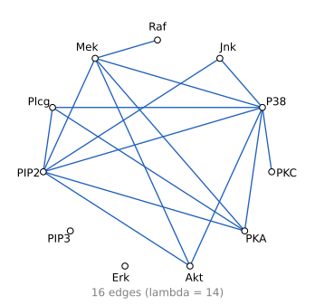
sachs.covmatrix (the sample covariance divided by 1000). The 16 edges are exactly those of the book's figure. PIP3 and Erk are isolated: on this scale their variances are about 2, small next to the penalty (see the note on scale). Code: fig_17_1. Reproduces Hastie, Tibshirani and Friedman (2009), Figure 17.1. Download: PDF · SVG17.2 Markov Graphs and Their Properties
pp. 627–630 This section is about what a graph says about a joint distribution; parametrisation and estimation come later.
See also (companion courses): Section 8.3.1, conditional independence properties of Markov random fields, and the d-separation demo, where separation in directed graphs is different (no explaining away here).
Definition 17.1 (graphs, paths, cliques) p. 627
A graph \(\Gc=(V,E)\) has a vertex set \(V\) and an edge set \(E\) of unordered pairs. Vertices \(X\) and \(Y\) are adjacent, \(X\sim Y\), if \(\{X,Y\}\in E\). A path is a sequence \(X_1,\dots,X_n\) with \(X_{i-1}\sim X_i\) for \(i=2,\dots,n\). A graph is complete if every pair of vertices is adjacent. A subgraph is a subset \(U\subseteq V\) with the edges among its vertices. A clique is a complete subgraph; it is maximal if no vertex can be added and keep it complete. For disjoint sets \(A,B,C\subseteq V\), \(C\) separates \(A\) and \(B\) if every path from a vertex of \(A\) to a vertex of \(B\) passes through a vertex of \(C\) (if no path joins \(A\) and \(B\), they are separated by the empty set).
Definition 17.2 (pairwise and global Markov properties) pp. 627–628, (17.1)–(17.2)
A distribution \(P\) of \(X_V\) is pairwise Markov with respect to \(\Gc\) if
\[ \text{no edge joining }X\text{ and }Y\ \Longrightarrow\ X\indep Y\given\rest, \tag{17.1} \]where "rest" is every other vertex, and globally Markov if for disjoint subsets \(A,B,C\)
\[ C\text{ separates }A\text{ and }B\ \Longrightarrow\ A\indep B\given C. \tag{17.2} \]The book writes (17.1) with a double arrow, but its own development only uses (and only can use, see the remark after Result 17.1) the direction shown: a missing edge implies independence.
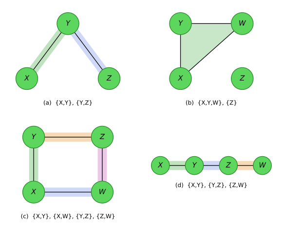
maximal_cliques) and agree with the book's: (a) \(\{X,Y\},\{Y,Z\}\); (b) \(\{X,Y,W\},\{Z\}\); (c) the four sides of the square; (d) the three links of the chain. Code: fig_17_2. Reproduces Hastie, Tibshirani and Friedman (2009), Figure 17.2. Download: PDF · SVGIn Figure 17.2(a), \(X\indep Z\given Y\). \(Y\) separates \(X\) and \(Z\) in (a) and (d); \(Z\) separates \(Y\) and \(W\) in (d); \(\{X,Z\}\) separates \(Y\) and \(W\) in (c); and in (b) the empty set separates \(Z\) from \(\{X,Y,W\}\), so \(Z\) is independent of the other three. The global property breaks a graph into conditionally independent pieces, which is the basis of exact computation on graphs.
Result 17.1 (pairwise and global Markov properties are equivalent for positive distributions) p. 628
(a) For every distribution, global Markov implies pairwise Markov. (b) If \(P\) has a density (or probability mass function) \(f>0\) everywhere on a product space, pairwise Markov implies global Markov.
Proof
(a) If \(X\) and \(Y\) are not adjacent, every path from \(X\) to \(Y\) has an interior vertex, all of which lie in "rest"; so rest separates them and (17.2) gives (17.1).
The intersection property. If \(f>0\), then \(X\indep Y\given(Z,W)\) and \(X\indep W\given(Z,Y)\) imply \(X\indep(Y,W)\given Z\). Indeed, positivity makes every conditional density well defined at every point, and the two assumptions say \(f(x\given y,z,w)=f(x\given z,w)\) and \(f(x\given y,z,w)=f(x\given z,y)\). Hence \(f(x\given z,w)=f(x\given z,y)\) for all \(y,w\); fixing \(y=y_0\) shows that \(f(x\given z,w)=a(x,z)\) does not depend on \(w\), so \(f(x\given y,z,w)=a(x,z)\), which is the claim. We also use decomposition: \(A\indep(B\cup D)\given C\) implies \(A\indep B\given C\) (integrate out \(D\)).
(b) We show by backward induction on \(|C|\) that \(A\indep B\given C\) whenever \(A,B\) are non-empty, \(A,B,C\) are disjoint and \(C\) separates \(A\) and \(B\). If \(|C|=p-2\), \(A\) and \(B\) are single non-adjacent vertices and this is (17.1). Suppose the claim holds for all separators larger than \(C\).
Case \(A\cup B\cup C=V\). One of \(A,B\) has two or more vertices (else \(|C|=p-2\)); say \(A\), and pick \(\alpha\in A\). The set \(C\cup\{\alpha\}\) separates \(A\setminus\{\alpha\}\) and \(B\), and \(C\cup(A\setminus\{\alpha\})\) separates \(\{\alpha\}\) and \(B\) (any path to \(B\) must cross \(C\)). By induction, \(A\setminus\{\alpha\}\indep B\given C\cup\{\alpha\}\) and \(\alpha\indep B\given C\cup(A\setminus\{\alpha\})\); the intersection property gives \(A\indep B\given C\).
Case \(A\cup B\cup C\ne V\). Pick \(\gamma\notin A\cup B\cup C\). Then \(C\cup\{\gamma\}\) separates \(A\) and \(B\), so \(A\indep B\given C\cup\{\gamma\}\). Also \(\gamma\) cannot be joined to both \(A\) and \(B\) by paths avoiding \(C\) (that would join \(A\) to \(B\) avoiding \(C\)); if it is not joined to \(A\), then \(B\cup C\) separates \(A\) and \(\gamma\), and by induction \(A\indep\gamma\given B\cup C\). The intersection property gives \(A\indep(B\cup\{\gamma\})\given C\), and decomposition gives \(A\indep B\given C\). The other case is symmetric. ∎
Why "for positive distributions". Let \(X_1=X_2=X_3\) be one fair coin and the graph have no edges. Given any one variable the other two are constants, so every pairwise statement holds, yet \(X_1\) and \(X_2\) are not independent: the global property fails. The intersection step is exactly what breaks.
For example, in Figure 17.2(d) the missing edge gives \(X\indep Z\given\{Y,W\}\); the global property gives the stronger \(X\indep Z\given Y\) and \(X\indep W\given Y\), and also \(Y\indep W\given Z\). In the precision-zeros demo you can pick any pair of a graph and see its smallest separating set and the conditional covariance (zero) given it.
Filling the gap 17.1: why the double arrow in (17.1) cannot hold in general p. 628
Derivation
Read as an equivalence, (17.1) would say that an edge forces dependence. But a graph's properties are implications only: every distribution in which all variables are independent is Markov with respect to every graph, including the complete one. What is true is that for "generic" parameters of a model on \(\Gc\) the edges are dependences. For the Gaussian, \(\theta_{jk}\ne0\) on an edge means \(X_j\) and \(X_k\) are dependent given the rest (Result 17.4); the converse statement is about the zero pattern of a particular \(\bTh\), not about the graph. The code checks the generic statement: for 20 random sparse precision matrices on 6 nodes, every separating set gives a conditional covariance below \(10^{-17}\), and every non-separating set gives one above \(10^{-9}\). ∎
The maximal cliques of Figure 17.2 are listed in its caption. Most computational methods first decompose a graph into cliques, compute within them and combine the results; the best known is the junction-tree algorithm for marginal probabilities (Lauritzen and Spiegelhalter, 1988; see Algorithm 8.6 of the companion course). The next result says which distributions are Markov on a graph.
See also (companion course): Section 8.3.2, factorization properties, where the theorem is proved in full.
Result 17.2 (Hammersley–Clifford; Hammersley and Clifford, 1971; Clifford, 1990) p. 629, (17.3)–(17.4)
Let \(f>0\) on a product space. Then \(f\) is (pairwise, equivalently globally) Markov with respect to \(\Gc\) if and only if
\[ f(x)=\frac1Z\prod_{C\in\Cc}\psi_C(x_C) \tag{17.3} \]for some positive functions \(\psi_C\) (the clique potentials) of the variables of the maximal cliques \(\Cc\), with normalising constant (partition function)
\[ Z=\sum_{x\in\Xc}\prod_{C\in\Cc}\psi_C(x_C) \tag{17.4} \](an integral for continuous variables).
Proof (factorisation implies Markov in full; the converse in outline)
(17.3) implies global Markov. Let \(C\) separate \(A\) and \(B\). Let \(\tilde A\) be the set of vertices joined to \(A\) by paths avoiding \(C\) (so \(A\subseteq\tilde A\)) and \(\tilde B=V\setminus(\tilde A\cup C)\supseteq B\). No clique contains a vertex of \(\tilde A\) and one of \(\tilde B\), since they would be adjacent and the second vertex would be in \(\tilde A\). So every clique lies in \(\tilde A\cup C\) or in \(\tilde B\cup C\), and grouping the factors gives \(f(x)=g(x_{\tilde A},x_C)\,h(x_{\tilde B},x_C)\). This factorisation is equivalent to \(X_{\tilde A}\indep X_{\tilde B}\given X_C\), and decomposition gives \(A\indep B\given C\). Positivity is not needed for this direction.
Pairwise Markov implies (17.3). Fix a reference point \(x^*\), and for \(S\subseteq V\) define \(H_S(x)=\sum_{U\subseteq S}(-1)^{|S\setminus U|}\log f(x_U,x^*_{V\setminus U})\) (finite because \(f>0\)). Möbius inversion gives \(\log f(x)=\sum_{S\subseteq V}H_S(x_S)\). If \(S\) contains two non-adjacent vertices \(j,k\), the pairwise property makes \(\log f\) a sum of a function without \(x_j\) and a function without \(x_k\) (given the rest), and the terms of \(H_S\) cancel in fours, so \(H_S\equiv0\). Hence only cliques carry terms, and grouping them into maximal cliques gives (17.3) with \(\psi_C=\exp(\sum H_S)\). The cancellation is written out in Result 8.13 of the companion course. ∎
Checked numerically: for a random positive Ising model on the four-cycle of Figure 17.2(c), all Möbius terms \(H_S\) with \(S\) not a clique are below \(3\times10^{-15}\).
Potentials are not densities in general (they need not be the marginals of their cliques); they are affinities that score some configurations of \(x_C\) above others. When the cliques are separated from each other, they can be taken to be densities (the book's footnote 1).
Filling the gap 17.2: a complete graph does not fix the order of interactions (17.5) pp. 629–630, Figure 17.3
On the complete graph with three nodes \(X,Y,Z\) (Figure 17.3 of the book, a triangle) both
\[ f^{(2)}(x,y,z)=\frac1Z\psi(x,y)\psi(x,z)\psi(y,z);\qquad f^{(3)}(x,y,z)=\frac1Z\psi(x,y,z) \tag{17.5} \]are Markov, since a complete graph asserts no independence.
Derivation
For binary variables, \(f^{(3)}\) is an arbitrary positive distribution on 8 cells: 7 free parameters. Taking logarithms, \(\log f^{(2)}\) is a sum of three functions of two binary arguments each; each has 4 values, and after removing redundant constants and main effects (which can be moved between factors) the model has 3 main effects and 3 two-way interactions: 6 free parameters. The missing parameter is the three-way interaction, the coefficient of \(xyz\) in \(\log f\); \(f^{(2)}\) is the "no second-order interaction" log-linear model for a \(2\times2\times2\) table (Bishop, Fienberg and Holland, 1975). So the graph cannot tell the two apart. Numerically, a random \(f^{(3)}\) projected by iterative proportional fitting onto the \(f^{(2)}\) family (matching its three two-way margins) stays at Kullback–Leibler distance 0.025 from it. ∎
The rest of the chapter uses pairwise Markov graphs: one potential per edge, so at most second-order interactions. They are parsimonious, easier to fit, have the least complexity compatible with the graph, and both the Gaussian and the binary models below depend on the data only through pairwise statistics.
17.3 Undirected Graphical Models for Continuous Variables
pp. 630–631 Assume \(X\sim N(\mu,\bSig)\). A Gaussian density is the exponential of a quadratic, so it has only pairwise interactions and is automatically a pairwise Markov graph model; Figure 17.1 is an example. All its conditionals are Gaussian, and \(\bTh=\bSig^{-1}\) holds the partial covariances.
See also (companion courses): Result 2.9, the conditional Gaussian, and Result 2.8, the partitioned inverse (Bayesian and Probabilistic Machine Learning); Result 3.7 (Foundations of Deep Learning).
Result 17.3 (the conditional distribution of one variable given the rest) p. 630, (17.6)–(17.7)
Write \(X=(Z,Y)\) with \(Z=(X_1,\dots,X_{p-1})\), \(Y=X_p\), and partition
\[ \bSig=\begin{pmatrix}\bSig_{ZZ}&\sigma_{ZY}\\ \sigma_{ZY}^\T&\sigma_{YY}\end{pmatrix}. \tag{17.7} \]Then
\[ Y\given Z=z\ \sim\ N\big(\mu_Y+(z-\mu_Z)^\T\bSig_{ZZ}^{-1}\sigma_{ZY},\ \sigma_{YY}-\sigma_{ZY}^\T\bSig_{ZZ}^{-1}\sigma_{ZY}\big). \tag{17.6} \]The conditional mean is the population linear regression of \(Y\) on \(Z\), with \(\beta=\bSig_{ZZ}^{-1}\sigma_{ZY}\) (as in (2.16)).
Proof sketch
Let \(\beta=\bSig_{ZZ}^{-1}\sigma_{ZY}\) and \(e=Y-\mu_Y-(Z-\mu_Z)^\T\beta\). Then \(\Cov(Z,e)=\sigma_{ZY}-\bSig_{ZZ}\beta=0\); since \((Z,e)\) is jointly Gaussian, \(e\) is independent of \(Z\), with variance \[ \sigma_{YY}-2\beta^\T\sigma_{ZY}+\beta^\T\bSig_{ZZ}\beta=\sigma_{YY}-\sigma_{ZY}^\T\bSig_{ZZ}^{-1}\sigma_{ZY}. \] So given \(Z=z\), \(Y=\mu_Y+(z-\mu_Z)^\T\beta+e\) with \(e\) still \(N(0,\cdot)\). The companion course derives the general case by completing the square. ∎
Result 17.4 (the precision matrix: regression coefficients and conditional independence) pp. 630–631, (17.8)–(17.9); Exercise 17.3
Partition \(\bTh=\bSig^{-1}\) like \(\bSig\). Then
\[ \theta_{ZY}=-\theta_{YY}\cdot\bSig_{ZZ}^{-1}\sigma_{ZY}, \tag{17.8} \]where \(1/\theta_{YY}=\sigma_{YY}-\sigma_{ZY}^\T\bSig_{ZZ}^{-1}\sigma_{ZY}>0\) is the conditional variance, and hence
\[ \beta=\bSig_{ZZ}^{-1}\sigma_{ZY}=-\theta_{ZY}/\theta_{YY}. \tag{17.9} \]Moreover, for any \(j\ne k\): \(\theta_{jk}=0\) if and only if \(X_j\indep X_k\given\rest\), and the partial correlation is \(\rho_{jk\given\rest}=-\theta_{jk}/\sqrt{\theta_{jj}\theta_{kk}}\).
Proof
(17.8). The last column of \(\bSig\bTh=\bI\) reads \(\bSig_{ZZ}\theta_{ZY}+\sigma_{ZY}\theta_{YY}=0\) and \(\sigma_{ZY}^\T\theta_{ZY}+\sigma_{YY}\theta_{YY}=1\). The first gives \(\theta_{ZY}=-\theta_{YY}\bSig_{ZZ}^{-1}\sigma_{ZY}\); substituting in the second gives \(\theta_{YY}(\sigma_{YY}-\sigma_{ZY}^\T\bSig_{ZZ}^{-1}\sigma_{ZY})=1\). The bracket is the conditional variance in (17.6), positive because \(\bSig\) is positive definite. Dividing (17.8) by \(-\theta_{YY}\) gives (17.9).
Zeros. By (17.9), the coefficient of \(X_k\) in the regression of \(X_j\) on the rest is \(-\theta_{jk}/\theta_{jj}\). By (17.6) the conditional distribution of \(X_j\) given the rest depends on \(x_k\) only through that coefficient, so \(\theta_{jk}=0\) iff the conditional law of \(X_j\) given the rest does not involve \(x_k\), which (Exercise 17.4) is \(X_j\indep X_k\given\rest\). Equivalently: the density is proportional to \(\exp\{-\frac12(x-\mu)^\T\bTh(x-\mu)\}\), and the only term involving both \(x_j\) and \(x_k\) is \(-\theta_{jk}(x_j-\mu_j)(x_k-\mu_k)\); the density factorises as \(g(x_j,\cdot)h(x_k,\cdot)\) iff that term vanishes.
Partial correlation. Exercise 17.3 shows that the conditional covariance of \((X_j,X_k)\) given the rest is \((\bTh_{aa})^{-1}\) with \(\bTh_{aa}=\begin{pmatrix}\theta_{jj}&\theta_{jk}\\ \theta_{jk}&\theta_{kk}\end{pmatrix}\), whose correlation is \(-\theta_{jk}/\sqrt{\theta_{jj}\theta_{kk}}\). ∎
So all the second-order information, structural (which entries are zero) and quantitative, sits in \(\bTh\), the natural parameter of the Gaussian, and the dependence structure can be learned by regressions. In the precision-zeros demo, a chain has a tridiagonal \(\bTh\) while every entry of \(\bSig\) is nonzero.
Filling the gap 17.3: the book's footnote 2, and covariance graphs p. 631
Derivation
Footnote 2. The footnote calls the distribution "arising from a Gaussian graphical model" a Wishart distribution. More precisely: if \(x_1,\dots,x_N\) are independent \(N(\mu,\bSig)\), then \(N\bS\) has a Wishart distribution with \(N-1\) degrees of freedom and scale \(\bSig\), with density proportional to \(\det(\bTh)^{(N-1)/2}\exp\{-\frac N2\Tr(\bS\bTh)\}\) as a function of \(\bTh\). Its log is \(\frac{N-1}2\log\det\bTh-\frac N2\Tr(\bS\bTh)\), which up to the factor \((N-1)/N\) on the first term is the partially maximised log-likelihood (17.11), an exponential family in the natural parameter \(\bTh\) with sufficient statistic \(\bS\). The data themselves are Gaussian; the sufficient statistic is Wishart.
Covariance graphs. In a covariance graph (relevance network) an edge means \(\sigma_{jk}\ne0\), i.e. marginal dependence. Zeros of \(\bSig\) are linear constraints on \(\bSig\), and the log-likelihood \(-\log\det\bSig-\Tr(\bS\bSig^{-1})\) is not concave in \(\bSig\) (it is concave in \(\bTh\)), so fitting a covariance graph is a non-convex problem with possibly several local maxima (Chaudhuri et al., 2007). ∎
17.3.1 Estimation of the Parameters when the Graph Structure is Known
pp. 631–634 Observations \(x_1,\dots,x_N\) are independent \(N(\mu,\bSig)\), and
\[ \bS=\frac1N\sum_{i=1}^N(x_i-\bar x)(x_i-\bar x)^\T \tag{17.10} \]is the empirical covariance matrix.
Result 17.5 (the Gaussian log-likelihood in \(\bTh\); concavity; the MLE is \(\bS\)) pp. 631–632, (17.11)
Maximised over \(\mu\) (at \(\hat\mu=\bar x\)), the log-likelihood is, up to the factor \(N/2\) and an additive constant,
\[ \ell(\bTh)=\log\det\bTh-\Tr(\bS\bTh). \tag{17.11} \]\(-\ell\) is convex on positive-definite matrices, with gradient \(\partial\ell/\partial\bTh=\bTh^{-1}-\bS\). If \(\bS\) is positive definite (almost surely when \(N>p\)), the unique maximiser is \(\hat\bTh=\bS^{-1}\), i.e. \(\hat\bSig=\bS\); if \(\bS\) is singular (for instance \(N\le p\)), \(\ell\) is unbounded above and there is no MLE.
Proof
Partial maximisation. The log-likelihood is \[ \frac N2\log\det\bTh-\frac12\sum_i(x_i-\mu)^\T\bTh(x_i-\mu)-\frac{Np}2\log2\pi. \] Writing \(x_i-\mu=(x_i-\bar x)+(\bar x-\mu)\), the cross terms sum to zero and \[ \sum_i(x_i-\mu)^\T\bTh(x_i-\mu)=N\Tr(\bS\bTh)+N(\bar x-\mu)^\T\bTh(\bar x-\mu), \] using \(a^\T\bTh a=\Tr(\bTh aa^\T)\). The last term is minimised by \(\mu=\bar x\), leaving \(\frac N2[\log\det\bTh-\Tr(\bS\bTh)]-\frac{Np}2\log2\pi\).
Derivative and concavity of \(\log\det\). For \(\bTh\succ0\) and symmetric \(\mathbf E\), write \(\bTh+t\mathbf E=\bTh^{1/2}(\bI+t\mathbf M)\bTh^{1/2}\) with \(\mathbf M=\bTh^{-1/2}\mathbf E\bTh^{-1/2}\), whose eigenvalues are \(m_1,\dots,m_p\). Then \[ \log\det(\bTh+t\mathbf E)=\log\det\bTh+\sum_i\log(1+tm_i). \] Its derivative at \(t=0\) is \(\sum_im_i=\Tr\mathbf M=\Tr(\bTh^{-1}\mathbf E)\), so the gradient is \(\bTh^{-1}\); its second derivative is \(-\sum_im_i^2\le0\), with equality only for \(\mathbf E=0\). So \(\log\det\) is strictly concave, and \(\Tr(\bS\bTh)\) is linear.
Maximiser. The gradient vanishes at \(\bTh^{-1}=\bS\). If \(\bS\succ0\), \(\hat\bTh=\bS^{-1}\) is a stationary point of a strictly concave function on a convex set, hence its unique maximiser. If \(\bS v=0\) for some unit vector \(v\), then along \(\bTh_t=\bI+tvv^\T\), \(\log\det\bTh_t=\log(1+t)\to\infty\) while \(\Tr(\bS\bTh_t)=\Tr\bS\) is constant. ∎
Now suppose some edges are missing, for example PIP3–Erk in Figure 17.1. Then the corresponding entries of \(\bTh\) are zero, and we maximise (17.11) subject to \(\theta_{jk}=0\) for \((j,k)\notin E\): an equality-constrained convex problem. Iterative proportional fitting (Speed and Kiiveri, 1986) and other methods using the clique decomposition exist (Whittaker, 1990; Lauritzen, 1996). The book proposes a regression-based method instead, whose real payoff comes in Section 17.3.2. The naive idea, regressing node \(j\) on its neighbours with the observed cross-products, ignores the constraints among the predictors; replacing the observed cross-product matrix by the current model estimate gives the exact constrained MLE.
Result 17.6 (the estimating equations for a known graph) pp. 632–633, (17.12)–(17.20)
With a Lagrange multiplier for each missing edge,
\[ \ell_C(\bTh)=\log\det\bTh-\Tr(\bS\bTh)-\sum_{(j,k)\notin E}\gamma_{jk}\theta_{jk}, \tag{17.12} \]whose stationarity condition is
\[ \bTh^{-1}-\bS-\bGam=0, \tag{17.13} \]with \(\bGam\) symmetric and zero on the diagonal and on the edges. Partition into part 1 (all but the last row and column) and part 2 (the last), and write \(\bW=\bTh^{-1}\). The upper-right block of (17.13) is
\[ \bw_{12}-\bs_{12}-\gamma_{12}=0, \tag{17.14} \]and from
\[ \begin{pmatrix}\bW_{11}&\bw_{12}\\ \bw_{12}^\T&w_{22}\end{pmatrix}\begin{pmatrix}\bTh_{11}&\theta_{12}\\ \theta_{12}^\T&\theta_{22}\end{pmatrix}=\begin{pmatrix}\bI&0\\0^\T&1\end{pmatrix} \tag{17.15} \]we get
\[ \bw_{12}=-\bW_{11}\theta_{12}/\theta_{22} \tag{17.16} \] \[ \phantom{\bw_{12}}=\bW_{11}\beta,\qquad\beta=-\theta_{12}/\theta_{22}. \tag{17.17} \]Substituting in (17.14),
\[ \bW_{11}\beta-\bs_{12}-\gamma_{12}=0. \tag{17.18} \]If node \(p\) has \(q\) neighbours, drop the \(p-1-q\) equations of the non-neighbours and the zero entries of \(\beta\), leaving the \(q\times q\) system
\[ \bW^*_{11}\beta^*-\bs^*_{12}=0, \tag{17.19} \]solved by \(\hat\beta^*=(\bW^*_{11})^{-1}\bs^*_{12}\) and padded with zeros. Finally
\[ \frac1{\theta_{22}}=w_{22}-\bw_{12}^\T\beta, \tag{17.20} \]and \(w_{22}=s_{22}\).
Proof
(17.13). By Result 17.5 the gradient of \(\log\det\bTh-\Tr(\bS\bTh)\) is \(\bTh^{-1}-\bS\), and that of \(\sum\gamma_{jk}\theta_{jk}\) is \(\bGam\) (with \(\gamma_{jk}=\gamma_{kj}\), each missing pair counted in both positions). The problem is concave with affine constraints, so (17.13) together with \(\theta_{jk}=0\) on the missing edges is necessary and sufficient for the constrained maximum (Boyd and Vandenberghe, 2004). Since \(\bGam\) vanishes on the diagonal and the edges, (17.13) says \(\bW=\bS\) there: the fitted covariance reproduces the sample covariance on every edge and on the diagonal, and is free elsewhere. In particular \(w_{22}=s_{22}\).
(17.16)–(17.17). The upper-right block of (17.15) is \(\bW_{11}\theta_{12}+\bw_{12}\theta_{22}=0\). Since \(\theta_{22}>0\) (a diagonal entry of a positive-definite matrix), \(\bw_{12}=-\bW_{11}\theta_{12}/\theta_{22}=\bW_{11}\beta\).
(17.19). \(\gamma_{12}\) has nonzero entries only at the non-neighbours of node \(p\), and there \(\theta_{12}\), hence \(\beta\), is zero. The rows of (17.18) at the neighbours do not involve \(\gamma\): they read \(\sum_{k\in E_p}(\bW_{11})_{jk}\beta_k=s_{jp}\) for \(j\in E_p\), which is (17.19). The rows at the non-neighbours only determine \(\gamma\), so they carry no information about \(\beta\).
(17.20). The bottom-right entry of (17.15) is \(\bw_{12}^\T\theta_{12}+w_{22}\theta_{22}=1\); dividing by \(\theta_{22}\) and using \(\theta_{12}=-\beta\theta_{22}\) gives \(w_{22}-\bw_{12}^\T\beta=1/\theta_{22}\). This is Exercise 17.6. ∎
Algorithm 17.1 (a modified regression algorithm for a Gaussian graphical model with known structure) p. 634
- Initialise \(\bW=\bS\).
- Repeat for \(j=1,2,\dots,p,1,2,\dots,p,\dots\) until convergence:
- Partition \(\bW\): part 1 is all but the \(j\)th row and column, part 2 the \(j\)th row and column.
- Solve \(\bW^*_{11}\beta^*-\bs^*_{12}=0\) for the coefficients of the neighbours of \(j\) (17.19); pad with zeros to get \(\hat\beta\).
- Update \(\bw_{12}=\bW_{11}\hat\beta\).
- In the final cycle, for each \(j\), set \(\hat\theta_{12}=-\hat\beta\cdot\hat\theta_{22}\) with \(1/\hat\theta_{22}=s_{22}-\bw_{12}^\T\hat\beta\).
The problem is not \(p\) separate regressions but \(p\) coupled ones; the common \(\bW\) in step (b) couples them. The book did not find the procedure in the literature; it is related to Dempster's (1972) covariance selection and to the iterative conditional fitting of Chaudhuri et al. (2007). The next result explains why it works.
Result 17.7 (Algorithm 17.1 is block coordinate ascent on the maximum-determinant completion) pp. 633–634
The dual of maximising (17.11) subject to \(\theta_{jk}=0\), \((j,k)\notin E\), is
\[ \max_{\bW\succ0}\ \log\det\bW\quad\text{subject to}\quad w_{jk}=s_{jk}\ \text{for } j=k \text{ and for } (j,k)\in E, \]and \(\hat\bW=\hat\bTh^{-1}\) is its solution: among all positive-definite matrices that agree with \(\bS\) on the diagonal and the edges, the fitted covariance has the largest determinant (Dempster, 1972). Steps (b)–(c) of Algorithm 17.1 maximise \(\log\det\bW\) exactly over the free entries of row and column \(j\), the others fixed. Hence \(\log\det\bW\) increases at every step, \(\bW\) stays positive definite, and the algorithm converges to \(\hat\bW\).
Proof
The dual. The Lagrangian of (17.12) is \(L(\bTh,\bGam)=\log\det\bTh-\Tr((\bS+\bGam)\bTh)\). For fixed \(\bGam\), Result 17.5 (with \(\bS+\bGam\) in place of \(\bS\)) gives \(\sup_\bTh L=-\log\det(\bS+\bGam)-p\) if \(\bS+\bGam\succ0\) (and \(+\infty\) otherwise). Minimising this over \(\bGam\) supported on the missing edges is maximising \(\log\det\bW\) over \(\bW=\bS+\bGam\), the stated problem. Strong duality holds because the primal has a strictly feasible point (\(\bTh=\bI\)), and at the optimum \(\hat\bW=\hat\bTh^{-1}\) by (17.13). Conversely, the gradient of \(\log\det\bW\) in a free entry \(w_{jk}\) is \(2(\bW^{-1})_{jk}\), so at the dual optimum \(\bW^{-1}\) has zeros on the missing edges: the maximum-determinant completion is exactly the constrained MLE.
The block step. With \(\bW_{11}\) and \(w_{22}=s_{22}\) fixed, the Schur complement gives \[ \log\det\bW=\log\det\bW_{11}+\log(w_{22}-\bw_{12}^\T\bW_{11}^{-1}\bw_{12}). \] Maximising over the free entries of \(\bw_{12}\) (those at non-neighbours) means minimising \(\bw_{12}^\T\bW_{11}^{-1}\bw_{12}\) with \((\bw_{12})_k=s_{kj}\) fixed at the neighbours \(k\). Substitute \(\bw_{12}=\bW_{11}\beta\): minimise \(\beta^\T\bW_{11}\beta\) subject to \((\bW_{11}\beta)_k=s_{kj}\) for neighbours \(k\). With multipliers \(\nu\), stationarity is \(2\bW_{11}\beta=\bW_{11}P\nu\), where \(P\) places \(\nu\) at the neighbours; so \(\beta=\frac12P\nu\) is zero at the non-neighbours, and the constraints become \(\bW^*_{11}\beta^*=\bs^*_{12}\). That is steps (b) and (c). The objective is a positive-definite quadratic, so this is the unique block maximiser.
Convergence. Each step does not decrease \(\log\det\bW\), which is bounded above by \(\sum_j\log s_{jj}\) (Hadamard's inequality), so \(\bW\) stays in a compact set of positive-definite matrices. A strictly concave function maximised exactly and uniquely over each block in turn converges to its maximiser (Bertsekas, 1999, Proposition 2.7.1). Step 3 then reads off \(\hat\bTh\) by (17.17) and (17.20). ∎
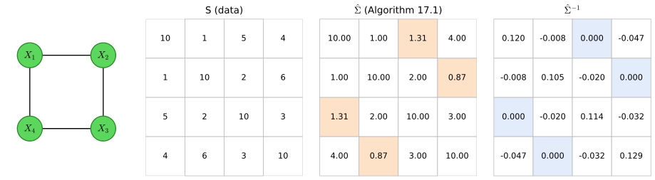
fig_17_4, modified_regression. Reproduces Hastie, Tibshirani and Friedman (2009), Figure 17.4, with the book's numerical example. Download: PDF · SVGFilling the gap 17.4: the example of Figure 17.4 in numbers p. 634
Derivation
For node 1 the neighbours are 2 and 4, so step (b) solves the \(2\times2\) system with \(\bW^*_{11}=\begin{pmatrix}w_{22}&w_{24}\\w_{42}&w_{44}\end{pmatrix}\) and right side \((s_{21},s_{41})=(1,4)\); variable 3 is left out. Starting from \(\bW=\bS\), the first sweep already moves \(w_{13}\) from 5 to 1.3130 and \(w_{24}\) from 6 to 0.8706, and after five sweeps nothing changes in the twelfth digit:
\[ \hat\bSig=\begin{pmatrix}10&1&1.3142&4\\1&10&2&0.8705\\1.3142&2&10&3\\4&0.8705&3&10\end{pmatrix},\qquad \hat\bSig^{-1}=\begin{pmatrix}0.1197&-0.0079&0&-0.0472\\-0.0079&0.1048&-0.0199&0\\0&-0.0199&0.1137&-0.0324\\-0.0472&0&-0.0324&0.1286\end{pmatrix}. \]The log-likelihood (17.11) rises at every sweep, and a general-purpose optimiser of (17.11) over the eight free entries of \(\bTh\) reaches the same value, \(-12.8949070824\). Among 200 random positive-definite matrices that agree with \(\bS\) except at (1,3) and (2,4), none has a larger determinant. All entries agree with the book's two-decimal display except \(\hat\theta_{22}=0.1048\), which the book prints as 0.11 (note). This is the "positive-definite completion" of \(\bS\). ∎
17.3.2 Estimation of the Graph Structure
pp. 635–638 Usually the edges are unknown, and an \(L_1\) (lasso) penalty is used to discover them.
See also (this course): Result 3.16, the optimality conditions of the lasso, and Result 3.30, the coordinate update; (companion course) Section 8.4.8, learning the graph structure.
Result 17.8 (neighbourhood selection; Meinshausen and Bühlmann, 2006) p. 635
Regress each variable on all the others with a lasso penalty, and declare \(\theta_{jk}\ne0\) if the coefficient of \(X_k\) for \(X_j\) or (alternatively and) that of \(X_j\) for \(X_k\) is nonzero. In the population, by (17.9) the coefficient of \(X_k\) for \(X_j\) is \(-\theta_{jk}/\theta_{jj}\), so its zero pattern is exactly that of \(\bTh\). Meinshausen and Bühlmann prove that with suitably chosen penalties the procedure recovers the set of nonzero \(\theta_{jk}\) with probability tending to one, even when \(p\) grows faster than \(N\), under a "neighbourhood stability" condition analogous to the lasso's irrepresentability condition (3.81).
The method estimates only the zero pattern, not \(\bTh\) or \(\bSig\). Run from the covariance matrix: the lasso \(\frac1{2N}\|y-\bZ\beta\|^2+\lambda\|\beta\|_1\) of a centred variable on the others equals \(\frac12\beta^\T\bS_{11}\beta-\bs_{12}^\T\beta+\lambda\|\beta\|_1\) plus a constant. At \(\lambda=0\) the code recovers \(-\theta_{jk}/\theta_{jj}\) to \(10^{-8}\); at \(\lambda=14\) on the flow data the "or" rule gives 10 edges and the "and" rule 5, against 16 for the graphical lasso at the same \(\lambda\).
A more systematic approach maximises the penalised log-likelihood
\[ \log\det\bTh-\Tr(\bS\bTh)-\lambda\|\bTh\|_1, \tag{17.21} \]where \(\|\bTh\|_1\) is the sum of the absolute values of all entries of \(\bTh=\bSig^{-1}\). Its negative is convex. In place of (17.13), a maximiser satisfies
\[ \bTh^{-1}-\bS-\lambda\cdot\Sign(\bTh)=0, \tag{17.22} \]with \(\Sign(\theta_{jk})=\sgn(\theta_{jk})\) if \(\theta_{jk}\ne0\) and \(\Sign(\theta_{jk})\in[-1,1]\) if \(\theta_{jk}=0\) (subgradient notation). The development of Section 17.3.1 leads to
\[ \bW_{11}\beta-\bs_{12}+\lambda\cdot\Sign(\beta)=0, \tag{17.23} \]which is exactly the estimating equation of a lasso. With response \(\by\) and predictors \(\bZ\), the lasso minimises
\[ \tfrac12(\by-\bZ\beta)^\T(\by-\bZ\beta)+\lambda\cdot\|\beta\|_1 \tag{17.24} \](this is (3.52) with a factor \(\frac12\)), whose subgradient equation is
\[ \bZ^\T\bZ\beta-\bZ^\T\by+\lambda\cdot\Sign(\beta)=0. \tag{17.25} \]So \(\bZ^\T\by\) plays the role of \(\bs_{12}\) (up to \(1/N\)) and the estimated cross-product matrix \(\bW_{11}\) replaces \(\bZ^\T\bZ\).
Result 17.9 (each block of the graphical lasso is a lasso) pp. 635–636, (17.22)–(17.27)
(a) The upper-right block of (17.22) is equivalent to (17.23) with \(\beta=-\theta_{12}/\theta_{22}\) and \(\bw_{12}=\bW_{11}\beta\). (b) For \(\bW_{11}\succ0\), the solutions of (17.23) are exactly the minimisers of the convex function
\[ g(\beta)=\tfrac12\beta^\T\bW_{11}\beta-\bs_{12}^\T\beta+\lambda\|\beta\|_1 . \](c) Minimising \(g\) over \(\beta_j\) with the other coordinates fixed gives, with \(\bV=\bW_{11}\),
\[ \hat\beta_j\leftarrow S\Big(s_{12j}-\sum_{k\ne j}V_{kj}\hat\beta_k,\ \lambda\Big)\Big/V_{jj}, \tag{17.26} \] \[ S(x,t)=\sgn(x)(|x|-t)_+ . \tag{17.27} \](d) The diagonal of the solution is \(w_{jj}=s_{jj}+\lambda\), which is why Algorithm 17.2 can fix it at the start.
Proof
(a) The upper-right block of (17.22) is \(\bw_{12}-\bs_{12}-\lambda\Sign(\theta_{12})=0\). As in Result 17.6, \(\bw_{12}=\bW_{11}\beta\) with \(\beta=-\theta_{12}/\theta_{22}\), and \(\theta_{22}>0\), so \(\beta\) and \(\theta_{12}\) have opposite signs entry by entry and \(\Sign(\theta_{12})=-\Sign(\beta)\) (as sets, including the interval \([-1,1]\) at zero). Substituting gives (17.23).
(b) \(g\) is the sum of a convex quadratic and a convex norm, and its subdifferential at \(\beta\) is \(\{\bW_{11}\beta-\bs_{12}+\lambda u:\ u\in\Sign(\beta)\}\). A point minimises a convex function iff 0 is a subgradient (Chapter 3, Filling the gap 3.7), which is (17.23). Expanding (17.24), \(\frac12\beta^\T\bZ^\T\bZ\beta-\beta^\T\bZ^\T\by+\lambda\|\beta\|_1+\frac12\by^\T\by\): the same form, which is the sense in which (17.23) is a lasso.
(c) As a function of \(\beta_j\) alone, \(g=\frac12V_{jj}\beta_j^2-\beta_jr_j+\lambda|\beta_j|+\text{const}\) with \(r_j=s_{12j}-\sum_{k\ne j}V_{kj}\beta_k\). For \(\beta_j>0\) the derivative \(V_{jj}\beta_j-r_j+\lambda\) vanishes at \(\beta_j=(r_j-\lambda)/V_{jj}\), admissible iff \(r_j>\lambda\); similarly \(\beta_j=(r_j+\lambda)/V_{jj}\) iff \(r_j<-\lambda\); and if \(|r_j|\le\lambda\) then \(0\in-r_j+\lambda[-1,1]\), so \(\beta_j=0\). Together: \(\beta_j=S(r_j,\lambda)/V_{jj}\). Cycling through the coordinates converges to the minimiser because the non-smooth part is separable (Tseng, 2001; Result 3.30).
(d) \(\bTh\succ0\) has \(\theta_{jj}>0\), so \(\Sign(\theta_{jj})=1\), and the diagonal of (17.22) reads \(w_{jj}-s_{jj}-\lambda=0\). In the variant of the book's footnote 3, where the diagonal is not penalised, the same argument gives \(w_{jj}=s_{jj}\). ∎
Algorithm 17.2 (graphical lasso; Friedman, Hastie and Tibshirani, 2008, building on Banerjee, El Ghaoui and d'Aspremont, 2008) p. 636
- Initialise \(\bW=\bS+\lambda\bI\). The diagonal of \(\bW\) is not changed afterwards.
- Repeat for \(j=1,2,\dots,p,1,2,\dots,p,\dots\) until convergence:
- Partition \(\bW\) into part 1 (all but row and column \(j\)) and part 2 (row and column \(j\)).
- Solve \(\bW_{11}\beta-\bs_{12}+\lambda\cdot\Sign(\beta)=0\) by the cyclical coordinate descent (17.26).
- Update \(\bw_{12}=\bW_{11}\hat\beta\).
- In the final cycle, for each \(j\), set \(\hat\theta_{12}=-\hat\beta\cdot\hat\theta_{22}\) with \(1/\hat\theta_{22}=w_{22}-\bw_{12}^\T\hat\beta\).
The book's statement that it "can be shown" that the algorithm gives the exact maximiser of (17.21) is the next result.
Result 17.10 (the dual of the graphical lasso; existence, uniqueness and convergence) p. 636
For \(\lambda>0\) the dual of (17.21) is
\[ \max_{\bW}\ \log\det\bW\quad\text{subject to}\quad |w_{jk}-s_{jk}|\le\lambda\ \text{ for all } j,k , \]a strictly concave problem on a compact set containing \(\bS+\lambda\bI\succ0\). It has a unique solution \(\hat\bW\), even when \(\bS\) is singular (\(p>N\)), and \(\hat\bTh=\hat\bW^{-1}\) is the unique maximiser of (17.21), with \(\Tr(\bS\hat\bTh)+\lambda\|\hat\bTh\|_1=p\). Steps (b)–(c) of Algorithm 17.2 maximise \(\log\det\bW\) exactly over row and column \(j\), so the dual objective increases at every step and the algorithm converges to \(\hat\bW\).
Proof
Duality. Write \(\lambda\|\bTh\|_1=\max_{\|\bU\|_\infty\le1}\lambda\Tr(\bU\bTh)\) for symmetric \(\bU\) (take \(u_{jk}=\sgn\theta_{jk}\)). Then (17.21) is \(\max_\bTh\min_\bU\ \log\det\bTh-\Tr((\bS+\lambda\bU)\bTh)\). The function is concave in \(\bTh\), linear in \(\bU\), and \(\bU\) ranges over a compact convex set, so the max and min can be exchanged (Sion's minimax theorem). For fixed \(\bU\), the inner maximum over \(\bTh\) is \(-\log\det(\bS+\lambda\bU)-p\) (Result 17.5), finite iff \(\bS+\lambda\bU\succ0\). So the dual is \(\min_\bU-\log\det(\bS+\lambda\bU)-p\), i.e. maximise \(\log\det\bW\) over \(\bW=\bS+\lambda\bU\), \(\|\bU\|_\infty\le1\).
Existence and uniqueness. The feasible set is closed and bounded, \(\log\det\) is continuous where finite and tends to \(-\infty\) at singular matrices, and the feasible point \(\bS+\lambda\bI\) is positive definite (here \(\lambda>0\) matters when \(\bS\) is singular); so a maximiser exists, and strict concavity makes it unique. At the saddle point \(\hat\bTh=\hat\bW^{-1}\), and \(\Tr(\hat\bW\hat\bTh)=p\) with \(\hat\bW=\bS+\lambda\hat\bU\), \(\Tr(\hat\bU\hat\bTh)=\|\hat\bTh\|_1\), gives \(\Tr(\bS\hat\bTh)+\lambda\|\hat\bTh\|_1=p\): zero duality gap.
The block step. With the rest fixed, maximising \(\log\det\bW\) over \(\bw_{12}\) means minimising \(\frac12\bw_{12}^\T\bW_{11}^{-1}\bw_{12}\) subject to \(\|\bw_{12}-\bs_{12}\|_\infty\le\lambda\) (Schur complement, as in Result 17.7). Its KKT conditions, with \(\beta=\bW_{11}^{-1}\bw_{12}\), are: \(\beta_k>0\Rightarrow w_k-s_k=-\lambda\); \(\beta_k<0\Rightarrow w_k-s_k=\lambda\); \(\beta_k=0\Rightarrow|w_k-s_k|\le\lambda\). That is \(\bw_{12}-\bs_{12}+\lambda\Sign(\beta)\ni0\) with \(\bw_{12}=\bW_{11}\beta\), which is (17.23). So the lasso of step (b) solves the box-constrained block problem exactly, and step (c) applies its solution. Convergence follows as in Result 17.7 (Banerjee et al., 2008). ∎
Numerically, at \(\lambda\in\{0.5,7,14,27,36\}\) on the flow data, the code's fits satisfy (17.22) to a relative \(2\times10^{-10}\), the duality identity to \(3\times10^{-13}\), and agree with R's glasso to a relative \(7\times10^{-13}\).
Result 17.11 (where the graph is empty, and how it splits) beyond the book; Witten, Friedman and Simon (2011), Mazumder and Hastie (2012)
(a) If \(\lambda\ge\lambda_{\max}=\max_{j\ne k}|s_{jk}|\), the graphical lasso solution is \(\hat\bTh=\diag\{1/(s_{jj}+\lambda)\}\): no edges. For \(\lambda<\lambda_{\max}\) there is at least one edge. (b) If the graph with edges \(\{(j,k):|s_{jk}|>\lambda\}\) has connected components \(V_1,\dots,V_m\), then \(\hat\bTh\) is block diagonal with these blocks (up to ordering), each block being the graphical lasso of the corresponding sub-matrix of \(\bS\).
Proof
(a) Try \(\bW=\diag(s_{jj}+\lambda)\), \(\bTh=\bW^{-1}\). The diagonal of (17.22) holds; off the diagonal \(\theta_{jk}=0\) and (17.22) requires \(w_{jk}-s_{jk}=-s_{jk}\in\lambda[-1,1]\), i.e. \(|s_{jk}|\le\lambda\). By uniqueness (Result 17.10) this is the solution. If \(\lambda<|s_{jk}|\) for some pair, a diagonal \(\bW\) violates (17.22), so the solution has an edge.
(b) Solve the graphical lasso separately on each block and assemble \(\bW\) and \(\bTh\) block diagonally. Within blocks (17.22) holds; between blocks \(\theta_{jk}=w_{jk}=0\) and \(|s_{jk}|\le\lambda\) (no thresholded edge joins different components), so (17.22) holds there too. By uniqueness this is the solution. (So the graphical-lasso graph has no edges between the thresholded components; that its components are exactly these is the other half of the cited theorem.) ∎
For the book's matrix \(\lambda_{\max}=92.42\) (Raf–Mek). At \(\lambda=7,14,27,36,50,70\) the components of the graphical-lasso graph and of the thresholded graph agree exactly.
Filling the gap 17.5: edge-specific penalties subsume Algorithm 17.1 pp. 636–637
Derivation
Replace \(\lambda\|\bTh\|_1\) by \(\sum_{j,k}\lambda_{jk}|\theta_{jk}|\). Every step above goes through with \(\lambda\) replaced entrywise: (17.26) thresholds coordinate \(k\) at \(\lambda_{jk}\), and the dual constraint is \(|w_{jk}-s_{jk}|\le\lambda_{jk}\). Take \(\lambda_{jj}=0\), \(\lambda_{jk}=0\) on the edges and \(\lambda_{jk}=\infty\) on the missing edges: the soft threshold sets \(\beta_k=0\) whenever \(\lambda_{jk}=\infty\) and does nothing where \(\lambda_{jk}=0\), so the coordinate descent solves (17.19) and Algorithm 17.2 becomes Algorithm 17.1. The dual becomes "\(w_{jk}=s_{jk}\) on the edges and diagonal, free elsewhere", which is Result 17.7. The code confirms this on the flow data: Algorithm 17.1 with the graph of Figure 17.1 agrees with R's glasso run with \(\rho=0\) and those entries forced to zero to a relative \(2\times10^{-13}\). ∎
Because each step is a warm-started lasso, the whole path in \(\lambda\) is cheap to compute. Figure 17.5 shows four solutions for the flow data; the graph thins out as \(\lambda\) grows.
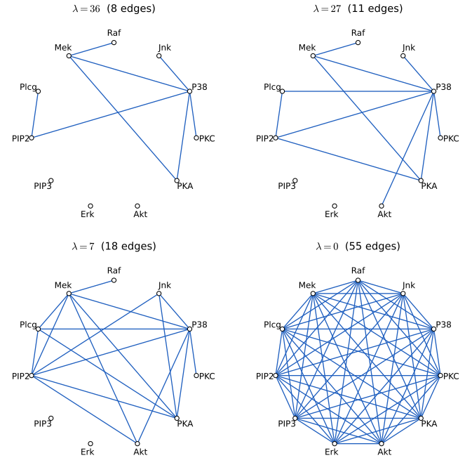
fig_17_5, glasso_path. Reproduces Hastie, Tibshirani and Friedman (2009), Figure 17.5. Download: PDF · SVG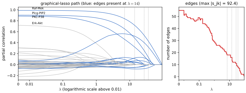
fig_17_s1. Download: PDF · SVGFinally, some nodes may be unobserved. If only some values at a node are missing, the EM algorithm can fill them in (Exercise 17.9). If a whole node is hidden, the Gaussian model gains nothing:
Result 17.12 (hidden Gaussian nodes) p. 638
If \(X=(X_V,X_H)\sim N(\mu,\bTh^{-1})\) and \(X_H\) is never observed, then \(X_V\) is Gaussian with covariance \(\bSig_{VV}\) and precision \(\bTh_{VV}-\bTh_{VH}\bTh_{HH}^{-1}\bTh_{HV}\). The model for the observed nodes is therefore a Gaussian whose precision matrix is "sparse minus low rank" (rank at most \(|H|\)): a subset of all Gaussians on \(V\), not an enlargement, and usually without zeros.
Proof
Marginals of Gaussians are Gaussian with the corresponding block of \(\bSig\). The partitioned-inverse formula (as in (17.8)) gives \((\bSig_{VV})^{-1}=\bTh_{VV}-\bTh_{VH}\bTh_{HH}^{-1}\bTh_{HV}\), the Schur complement of \(\bTh_{HH}\). The subtracted matrix has rank at most \(|H|\). For example, one hidden node joined to four observed nodes that are not joined to each other (a star) gives an observed precision with all six off-diagonal entries nonzero: the observed graph is complete although no two observed nodes share an edge. In the discrete case the nonlinearity makes hidden units genuinely enlarge the model (Section 17.4.2). ∎
17.4 Undirected Graphical Models for Discrete Variables
pp. 638–639 Pairwise Markov networks with binary nodes are the most common discrete models: Ising models in statistical mechanics, Boltzmann machines in machine learning, where the nodes are "units" that may be visible or hidden, often arranged in layers as in a neural network. They suit structured inputs such as images but are computationally demanding. First, all \(p\) nodes are visible, with edges \(E\).
See also (companion courses): the Ising prior for image de-noising, Filling the gap 8.9 and the image de-noising demo; energy-based models, Definition 14.2 of Foundations of Deep Learning.
Definition 17.3 (the Ising model) p. 638, (17.28)–(17.29)
For \(X\in\Xc=\{0,1\}^p\),
\[ p(X,\bTh)=\exp\Big[\sum_{(j,k)\in E}\theta_{jk}X_jX_k-\Phi(\bTh)\Big], \tag{17.28} \] \[ \Phi(\bTh)=\log\sum_{x\in\Xc}\Big[\exp\Big(\sum_{(j,k)\in E}\theta_{jk}x_jx_k\Big)\Big], \tag{17.29} \]where the edge set includes a constant node \(X_0\equiv1\) joined to every node, so that \(\theta_{j0}X_j\) are node (main-effect) terms. Since \(x_j^2=x_j\) for binary \(x_j\), the code stores \(\theta_{j0}\) on the diagonal of a symmetric \(p\times p\) matrix \(\bTh\).
The terms \(\theta_{jk}X_jX_k\) are a particular parametrisation of the log potentials of the edges, and \(\Phi\) is the log partition function. In statistics this is the Poisson log-linear model with first-order interactions for a \(2^p\) table of counts (Bishop et al., 1975; McCullagh and Nelder, 1989; Agresti, 2002). Why the constant node is needed is Exercise 17.10: without it the model cannot even fit the margins.
Result 17.13 (the Ising model has logistic conditionals; Exercise 17.11) p. 639, (17.30)
\[ \Pr(X_j=1\given X_{-j}=x_{-j})=\frac1{1+\exp\big(-\theta_{j0}-\sum_{(j,k)\in E}\theta_{jk}x_k\big)}, \tag{17.30} \]where \(X_{-j}\) is every node except \(j\). So \(\theta_{jk}\) is the log odds ratio for \(X_j\) and \(X_k\) given all the other nodes, and \(\theta_{jk}=0\) iff \(X_j\indep X_k\given\rest\).
Proof
Let \(x^1\) and \(x^0\) agree with \(x_{-j}\) and have \(x_j=1\) and \(x_j=0\). Every term of (17.28) without \(x_j\) and \(\Phi\) cancel in the ratio \(p(x^1)/p(x^0)=\exp(\theta_{j0}+\sum_{k:(j,k)\in E}\theta_{jk}x_k)\). Since \(\Pr(X_j=1\given x_{-j})=p(x^1)/(p(x^1)+p(x^0))\), dividing through by \(p(x^1)\) gives (17.30). The log odds of \(X_j\) is linear in \(x_k\) with slope \(\theta_{jk}\), which is the conditional log odds ratio; the conditional law of \(X_j\) given the rest is free of \(x_k\) iff \(\theta_{jk}=0\), and Exercise 17.4 turns that into conditional independence. ∎
17.4.1 Estimation of the Parameters when the Graph Structure is Known
pp. 639–641 With observations \(x_i\in\{0,1\}^p\), \(i=1,\dots,N\), the log-likelihood is
\[ \ell(\bTh)=\sum_{i=1}^N\log\Pr\nolimits_\bTh(X_i=x_i)=\sum_{i=1}^N\Big[\sum_{(j,k)\in E}\theta_{jk}x_{ij}x_{ik}-\Phi(\bTh)\Big]. \tag{17.31} \]Result 17.14 (gradient, Hessian and moment matching) pp. 639–640, (17.32)–(17.35)
The gradient is
\[ \frac{\partial\ell(\bTh)}{\partial\theta_{jk}}=\sum_{i=1}^Nx_{ij}x_{ik}-N\frac{\partial\Phi(\bTh)}{\partial\theta_{jk}}, \tag{17.32} \] \[ \frac{\partial\Phi(\bTh)}{\partial\theta_{jk}}=\sum_{x\in\Xc}x_jx_k\cdot p(x,\bTh)=\E_\bTh(X_jX_k), \tag{17.33} \]so the maximum-likelihood equations are
\[ \hat\E(X_jX_k)-\E_\bTh(X_jX_k)=0, \tag{17.34} \] \[ \hat\E(X_jX_k)=\frac1N\sum_{i=1}^Nx_{ij}x_{ik}. \tag{17.35} \]The Hessian is \(-N\Cov_\bTh(T)\), with \(T=(X_jX_k)_{(j,k)\in E}\) the sufficient statistics; it is negative definite, so \(\ell\) is strictly concave and has at most one maximiser, which exists iff the observed moments lie in the interior of the convex hull of \(\{T(x):x\in\Xc\}\) (for example when every cell of the \(2^p\) table has a positive count).
Proof
(17.32) is immediate from (17.31). For (17.33), \[ \frac{\partial\Phi}{\partial\theta_{jk}}=\frac{\sum_xx_jx_ke^{\sum\theta x x}}{\sum_xe^{\sum\theta x x}}=\sum_xx_jx_kp(x,\bTh). \] Differentiating once more, \[ \frac{\partial^2\Phi}{\partial\theta_a\partial\theta_b}=\E(T_aT_b)-\E(T_a)\E(T_b)=\Cov(T_a,T_b). \] A covariance matrix is positive semidefinite, and \(c^\T\Cov(T)c=\Var(c^\T T)=0\) would make \(c^\T T(x)\) constant on all of \(\{0,1\}^p\), impossible for \(c\ne0\) because the monomials \(x_jx_k\) (and \(x_j\)) are linearly independent functions on \(\{0,1\}^p\) together with the constant. So \(\Phi\) is strictly convex and \(\ell=\sum_i\theta^\T T(x_i)-N\Phi\) strictly concave. This is the general exponential-family fact that maximum likelihood sets sufficient statistics equal to their expectations; existence is Barndorff-Nielsen's (1978) condition. ∎
Checked: the gradient agrees with finite differences of the exact log-likelihood to \(10^{-9}\), and on the dichotomised flow data Newton's method reaches the maximum (average log-likelihood \(-6.7995\) per cell, against \(-11\log2=-7.6246\) for independent fair coins) in 7 steps, matching all 66 moments to \(3\times10^{-15}\).
For small \(p\) the moments \(\E_\bTh(X_jX_k)\) can be computed by enumerating the \(2^p\) states (strictly, the \(2^{p-2}\) with \(x_j=x_k=1\)), which is infeasible beyond about \(p=30\). The book lists three exact approaches:
Result 17.15 (Poisson log-linear models and iterative proportional fitting) p. 640; Exercise 17.12
(a) Poisson regression. Treat the \(2^p\) cell counts \(y\) as independent Poisson responses with \(\log\mu(x)=\theta_{00}+\sum_{(j,k)\in E}x_jx_k\theta_{jk}\). The Poisson maximum-likelihood estimates of \(\theta_{jk}\) are the Ising estimates, and \(\hat\theta_{00}=\log N-\Phi(\hat\bTh)\). The design has \(2^p\) rows and \(1+p+|E|\) columns (at most \(1+p+p(p-1)/2\)), so a Newton (IRLS) step costs \(O(p^42^p)\).
(b) Gradient ascent needs \(O(p^22^{p-2})\) per gradient but more steps.
(c) Iterative proportional fitting solves one equation of (17.34) exactly at a time. If the current model gives \(m=\E_\bTh(X_jX_k)\) and the data \(q=\hat\E(X_jX_k)\), the update is
Proof
(a) is Exercise 17.12, solved below. (c) Raising \(\theta_{jk}\) by \(\delta\) multiplies the unnormalised probability of every \(x\) with \(x_jx_k=1\) by \(e^\delta\) and leaves the others. So the new moment is \(me^\delta/(1-m+me^\delta)\); setting it equal to \(q\) and solving gives \(e^\delta=q(1-m)/(m(1-q))\). The same formula updates the node terms (\(x_j^2=x_j\)). Each step maximises \(\ell\) over one coordinate, so the likelihood never decreases. ∎
On the dichotomised flow data, statsmodels' Poisson GLM reproduces the Newton estimates to \(10^{-13}\), and IPF increases the likelihood at every sweep, ending 60 sweeps \(3\times10^{-4}\) below the maximum: one sweep costs about as much as a gradient, and convergence is linear, slower when the parameters are strongly coupled.
For \(p>30\) the gradient must be approximated. The mean-field approximation (Peterson and Anderson, 1987) replaces \(\E_\bTh(X_jX_k)\) by \(\E_\bTh(X_j)\E_\bTh(X_k)\) and solves the self-consistency equations \(m_j=\sigma(\theta_{j0}+\sum_k\theta_{jk}m_k)\) (the book's text has a typo here, see note). Gibbs sampling (Section 8.6) gives near-exact answers by sampling each node in turn from (17.30). On the fitted flow-data model, mean field misses some \(\E(X_jX_k)\) by 0.17 while 20000 Gibbs sweeps are within 0.01. Decomposable models (for instance trees) have closed-form estimates and avoid these problems (Whittaker, 1990, Chapter 12).
17.4.2 Hidden Nodes
pp. 641–642 Let \(X_\mathcal{H}\) be hidden and \(X_\mathcal{V}\) visible. Unlike the Gaussian case, hidden units make a discrete model richer.
Result 17.16 (the likelihood and gradient with hidden units) pp. 641–642, (17.36)–(17.38)
The observed-data log-likelihood is
\[ \ell(\bTh)=\sum_{i=1}^N\log\Big[\sum_{x_\mathcal{H}\in\Xc_\mathcal{H}}\exp\Big(\sum_{(j,k)\in E}\theta_{jk}x_{ij}x_{ik}\Big)\Big]-N\Phi(\bTh), \](the book's (17.36) places \(\Phi\) inside the sum over edges; see note), where in each term the hidden coordinates of \(x_i\) are the summation variables. Its gradient, divided by \(N\), is
\[ \frac1N\frac{\partial\ell(\bTh)}{\partial\theta_{jk}}=\hat\E_\mathcal{V}\E_\bTh(X_jX_k\given X_\mathcal{V})-\E_\bTh(X_jX_k), \tag{17.37} \]where for observation \(i\)
\[ \E_\bTh(X_jX_k\given X_\mathcal{V}=x_{i\mathcal{V}})=\begin{cases}x_{ij}x_{ik}&j,k\in\mathcal{V}\\ x_{ij}\Pr_\bTh(X_k=1\given X_\mathcal{V}=x_{i\mathcal{V}})&j\in\mathcal{V},\ k\in\mathcal{H}\\ \Pr_\bTh(X_j=1,X_k=1\given X_\mathcal{V}=x_{i\mathcal{V}})&j,k\in\mathcal{H}.\end{cases} \tag{17.38} \]Proof
\(\Pr(X_\mathcal{V}=x_{i\mathcal{V}})=\sum_{x_\mathcal{H}}p(x_{i\mathcal{V}},x_\mathcal{H})\), and \(\log p=\sum\theta xx-\Phi\) with \(\Phi\) not depending on \(x_\mathcal{H}\), so \(\Phi\) comes out of the sum once per observation. Differentiating \(\log\sum_{x_\mathcal{H}}e^{F(x_\mathcal{H})}\) gives \(\sum_{x_\mathcal{H}}\frac{e^F}{\sum e^F}\partial F/\partial\theta_{jk}\), and \(e^F/\sum e^F=\Pr_\bTh(x_\mathcal{H}\given x_{i\mathcal{V}})\) while \(\partial F/\partial\theta_{jk}=x_jx_k\). So the first term is \(\sum_i\E_\bTh(X_jX_k\given X_\mathcal{V}=x_{i\mathcal{V}})\), the "impute, then average" of the book (this is Fisher's identity, the same calculation as the E-step of EM). The second term is \(N\,\E_\bTh(X_jX_k)\) by (17.33). (17.38) uses that a visible \(x_{ij}\) is a constant given \(X_\mathcal{V}\) and that for binary variables \(\E(X_k\given\cdot)=\Pr(X_k=1\given\cdot)\) and \(\E(X_jX_k\given\cdot)=\Pr(X_j=X_k=1\given\cdot)\). ∎
Two Gibbs runs are needed: one from the model, for \(\E_\bTh(X_jX_k)\), and one for each training case with the visible units clamped at their values, for the conditional expectations, and both at every gradient step. This is very slow, which motivates the restrictions of Section 17.4.4.
17.4.3 Estimation of the Graph Structure
pp. 642–643 Lee et al. (2007) maximise the \(L_1\)-penalised log-likelihood exactly by conjugate gradients; the bottleneck is again \(\E_\bTh(X_jX_k)\), manageable for sparse graphs by the junction tree. Wainwright, Ravikumar and Lafferty (2007) approximate instead, in the spirit of neighbourhood selection.
Result 17.17 (node-wise \(L_1\) logistic regressions) p. 642
By (17.30), the regression of \(X_j\) on the other nodes is a logistic regression with coefficients \(\theta_{jk}\). Fit an \(L_1\)-penalised logistic regression for each node, giving \(\tilde\theta_{jk}\) (node \(j\) as outcome) and \(\tilde\theta_{kj}\) (node \(k\) as outcome), and symmetrise: the "min" rule takes the one smaller in absolute value, the "max" rule the larger. Under incoherence conditions both recover the edge set with probability tending to one (Wainwright et al., 2007), and they never compute \(\E_\bTh(X_jX_k)\), so dense graphs are no harder.
Unlike the Gaussian case, here \(\bTh\) itself is the object of interest (there is no covariance to invert), so the node-wise approximation estimates exactly what is wanted. Hoefling and Tibshirani (2008) found the approximations only slightly worse than the exact penalised fit. On the dichotomised flow data with eleven nodes, where the exact fit is cheap, the comparison is:
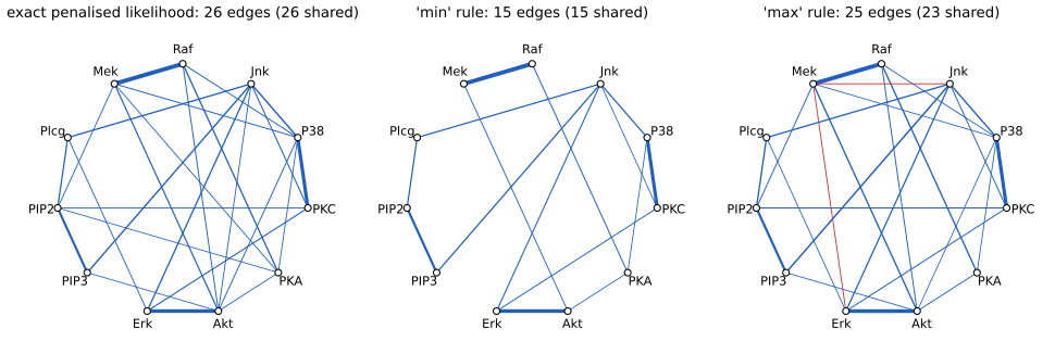
fig_17_s2, ising_l1, wainwright. Download: PDF · SVG17.4.4 Restricted Boltzmann Machines
pp. 643–645 A restricted Boltzmann machine (RBM) has one layer of visible and one layer of hidden units, with no connections inside a layer. In Figure 17.6 the visible layer is split into features \(V_1\) and labels \(V_2\), written
\[ V_1\leftrightarrow H\leftrightarrow V_2 . \tag{17.39} \]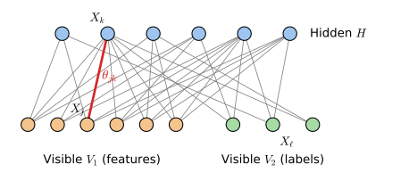
fig_17_6. Reproduces Hastie, Tibshirani and Friedman (2009), Figure 17.6. Download: PDF · SVGFor example \(V_1\) could be the binary pixels of a handwritten digit and \(V_2\) ten label units.
Result 17.18 (what the restriction buys: factorised conditionals and free energies) pp. 643–644
Write the RBM as \(p(v,h)\propto\exp(b^\T v+c^\T h+v^\T\bW h)\) (biases \(b,c\) from the constant node). Then (a) given \(v\) the hidden units are independent with \(\Pr(h_j=1\given v)=\sigma(c_j+v^\T\bW_{\cdot j})\), and given \(h\) the visible units are independent with \(\Pr(v_i=1\given h)=\sigma(b_i+\bW_{i\cdot}h)\); (b) the hidden units can be summed out:
\[ \sum_hp(v,h)\propto\exp\{-F(v)\},\qquad -F(v)=b^\T v+\sum_j\log\big(1+e^{c_j+v^\T\bW_{\cdot j}}\big); \](c) with a one-of-ten label unit \(y\), \(\Pr(y\given x)=e^{-F(x,y)}/\sum_{y'}e^{-F(x,y')}\), which needs no partition function.
Proof
(a) Given \(v\), \(\log p(v,h)=\text{const}+\sum_jh_j(c_j+v^\T\bW_{\cdot j})\) is a sum of terms each involving one \(h_j\), so \(p(h\given v)\) factorises, and each factor is the logistic of its coefficient (as in (17.30)). The case given \(h\) is symmetric. This is why all units of a layer can be sampled at once: one Gibbs "sweep" is two block updates, and the clamped expectations (17.38) are available in closed form, \(\E(v_ih_j\given v)=v_i\sigma(c_j+v^\T\bW_{\cdot j})\).
(b) \(\sum_{h\in\{0,1\}^H}e^{b^\T v+\sum_jh_ja_j}=e^{b^\T v}\prod_j(1+e^{a_j})\) with \(a_j=c_j+v^\T\bW_{\cdot j}\), because the sum of a product of independent factors is the product of their sums.
(c) \(\Pr(y\given x)=p(x,y)/\sum_{y'}p(x,y')\); the partition function is common to numerator and denominator and cancels. This is the book's "comparing the unnormalised joint densities of each label category". ∎
Checked: for a small RBM, summing the hidden units by brute force agrees with (b) to \(10^{-10}\), the conditional of \(h\) given \(v\) factorises to \(10^{-14}\), and (c) agrees with enumeration to \(10^{-14}\).
An RBM has the same shape as a single-hidden-layer neural network (Section 11.3), but its edges are undirected, its hidden units binary and random, and it is fitted by maximising the likelihood of all visible units (features and labels) rather than the conditional likelihood of the labels. It can therefore spend hidden units on structure in the features that has nothing to do with the labels, which may help when such features are combined with other layers.
Gibbs sampling in an RBM can take a long time to reach stationarity, and longer as the weights grow. Hinton (2002) found that learning works well if the model expectation in (17.37) is estimated by starting the chain at the data and running only a few steps: sample \(H\) given \(V_1,V_2\), then \(V_1,V_2\) given \(H\), then \(H\) given \(V_1,V_2\) again. This is contrastive divergence.
See also (companion course): Result 14.14, the likelihood gradient of an energy-based model, and Result 14.18, what contrastive divergence optimises, in Foundations of Deep Learning.
Result 17.19 (contrastive divergence CD-\(k\)) p. 644; Hinton (2002)
Let \(p^0\) be the empirical distribution of the visible data and \(p^k\) the distribution after \(k\) full Gibbs sweeps started from \(p^0\). CD-\(k\) replaces the model term \(\E_\bTh(X_jX_k)\) of (17.37) by its expectation under \(p^k\) (with the last hidden layer entering through its probabilities). (a) As \(k\to\infty\), \(p^k\) tends to the model distribution and CD-\(k\) to the exact gradient. (b) If the data distribution equals a model distribution \(p_\bTh\), the CD update has expectation zero at \(\bTh\): the true parameter is a fixed point. (c) In general CD is not the gradient of any objective; it approximates the gradient of \(\mathrm{KL}(p^0\|p_\bTh)-\mathrm{KL}(p^k\|p_\bTh)\) with one term dropped, and its fixed points differ (usually slightly) from the maximum-likelihood estimate (Carreira-Perpiñán and Hinton, 2005).
Proof
(a) Every conditional is strictly between 0 and 1, so the Gibbs chain on the finite state space is irreducible and aperiodic with stationary distribution \(p_\bTh\) (Result 8.10); hence \(p^k\to p_\bTh\) and the CD expectation tends to \(\E_\bTh\). (b) If \(p^0=p_\bTh\), the chain starts in its stationary distribution and stays there, so \(p^k=p^0\) and the data and "model" terms are equal in expectation. (c) The derivation of the approximate objective, and why the dropped term is usually small, is Result 14.18 of the companion course. ∎
Because this chapter's binary example has only 2048 visible states, the exact gradient and the exact likelihood can be computed alongside CD (Figure 17.S3). Both fits start from the same point with the same steps.
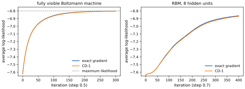
fig_17_s3, train_boltzmann. Download: PDF · SVGThe book's example trains an RBM by contrastive divergence on the MNIST digits (LeCun et al., 1998) with 2000 hidden units, 784 binary pixel units and one ten-way label unit, reaching 1.9% test error (a support vector machine: 1.4%). Replacing the pixels by 500 features from an RBM trained on images alone, whose hidden states feed a second 500-unit RBM, whose states in turn feed the 2000-unit joint model, lowers the error to 1.25%; this greedy layer-wise learning is described in Hinton, Osindero and Teh (2006).
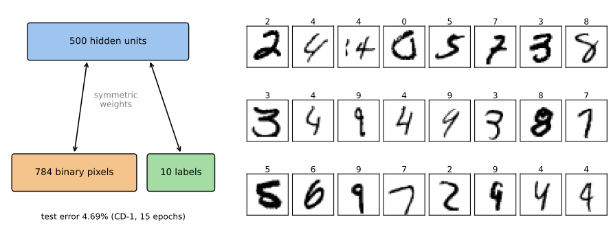
fig_17_7, mnist_rbm. Reproduces Hastie, Tibshirani and Friedman (2009), Figure 17.7, in reduced form. Download: PDF · SVGNotes on the book
Note on the book: one entry of \(\hat\bSig^{-1}\) on p. 634
The example after Figure 17.4 prints the \((2,2)\) entry of \(\hat\bSig^{-1}\) as 0.11. Algorithm 17.1, a general-purpose optimiser and the maximum-determinant characterisation all give 0.1048, which rounds to 0.10. Every other printed entry of \(\hat\bSig\) and \(\hat\bSig^{-1}\) is reproduced to the book's two decimals (Filling the gap 17.4).
Note on the book: the mean-field approximation, p. 641
The text says that mean field estimates \(\E_\bTh(X_jX_k)\) by \(\E_\bTh(X_j)\E_\bTh(X_j)\); the second factor should be \(\E_\bTh(X_k)\).
Note on the book: equations (17.36) and (17.37)
In (17.36) the log partition function is written inside the sum over edges, \(\sum_{(j,k)\in E}(\theta_{jk}x_{ij}x_{ik}-\Phi(\bTh))\), which would subtract \(\Phi\) once per edge and put it inside the sum over the hidden states. It belongs outside (Result 17.16): \[ \ell=\sum_i\log\sum_{x_\mathcal{H}}\exp\Big(\sum_E\theta_{jk}x_{ij}x_{ik}\Big)-N\Phi(\bTh). \] Also, (17.37) is the gradient of \(\ell/N\), not of \(\ell\) as written; compare (17.32), which keeps the factor \(N\).
Note on the book: Exercise 17.5
The exercise refers to "the setup in Section 17.4.1"; the equations \(\bS_{11}\beta-\bs_{12}=0\) belong to the Gaussian setup of Section 17.3.1.
Note on the book: the correction term in Exercise 17.9
In (17.44) the correction \(c_{i,jj'}\) is given as \(\hat\Sigma_{jj'}\) for \(j,j'\in m_i\). The expected cross-product of two missing values is \(\hat x_{ij}\hat x_{ij'}\) plus their conditional covariance given the observed values, \(\hat\Sigma_{jj'}-\hat\bSig_{j,o_i}\hat\bSig_{o_i,o_i}^{-1}\hat\bSig_{o_i,j'}\), not \(\hat\Sigma_{jj'}\) (Little and Rubin, 2002). Using \(\hat\Sigma_{jj'}\) counts the explained part of the variance twice: in the code's run of Exercise 17.9(c) it inflates the fitted variance of Jnk from 48803 to 53479 (data scale). Also, the second factor of (17.44) should read \((\hat x_{ij'}-\hat\mu_{j'})\).
Note on the book: "up to \(1+p+p^2\) columns", p. 640, and footnote 2, p. 631
The Poisson design for the pairwise model has \(1+p+p(p-1)/2\) columns (an intercept, \(p\) node terms and one column per pair), so \(p^2\) is a loose bound. Footnote 2's "the distribution arising from a Gaussian graphical model is a Wishart distribution" refers to the sampling distribution of \(N\bS\), not to the data (Filling the gap 17.3).
Note on the book: the penalty is applied on the covariance scale
The values \(\lambda=0,7,14,27,36\) of Figures 17.1 and 17.5 refer to the file sachs.covmatrix on the book's website, which is the sample covariance of the raw measurements divided by 1000 (confirmed against sachs.data to \(10^{-4}\)); with that matrix the code reproduces the book's edge sets exactly. The \(L_1\) penalty is not scale invariant: proteins with small variance (PIP3 and Erk, about 2, against 415 for PKA) have large precision entries and are penalised away first, which is why they are isolated in Figure 17.1 although Erk–Akt and PIP2–PIP3 have unpenalised partial correlations 0.72 and 0.90. On the correlation scale (each protein standardised) the graph with 16 edges contains both (demo preset 4). Neither choice is wrong, but the graph depends on it.
Exercises
All 12 exercises of Chapter 17 (Hastie, Tibshirani and Friedman, 2009, pp. 645–648), restated in my own words, with complete solutions (hidden).
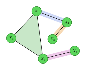
fig_17_8. Reproduces Hastie, Tibshirani and Friedman (2009), Figure 17.8. Download: PDF · SVGExercise 17.1. For the graph of Figure 17.8, list the conditional independences it implies and find its maximal cliques.
Solution
Maximal cliques: \(\{X_1,X_2,X_6\}\), \(\{X_1,X_4\}\), \(\{X_3,X_4\}\), \(\{X_5,X_6\}\).
Pairwise (17.1): the nine non-adjacent pairs give \(X_j\indep X_k\given\rest\) for \((j,k)\) = (1,3), (1,5), (2,3), (2,4), (2,5), (3,5), (3,6), (4,5), (4,6).
Local: each node is independent of its non-neighbours given its neighbours: \(X_1\indep\{X_3,X_5\}\given\{X_2,X_4,X_6\}\); \(X_2\indep\{X_3,X_4,X_5\}\given\{X_1,X_6\}\); \(X_3\indep\{X_1,X_2,X_5,X_6\}\given X_4\); \(X_4\indep\{X_2,X_5,X_6\}\given\{X_1,X_3\}\); \(X_5\indep\{X_1,\dots,X_4\}\given X_6\); \(X_6\indep\{X_3,X_4\}\given\{X_1,X_2,X_5\}\).
Global (17.2): every separation gives an independence; the smallest separators of the non-adjacent pairs are \(X_1\indep X_3\given X_4\); \(X_1\indep X_5\given X_6\); \(X_2\indep X_3\given X_1\) (or \(X_4\)); \(X_2\indep X_4\given X_1\); \(X_2\indep X_5\given X_6\); \(X_3\indep X_5\given X_1\) (or \(X_4\), or \(X_6\)); \(X_3\indep X_6\given X_1\) (or \(X_4\)); \(X_4\indep X_5\given X_1\) (or \(X_6\)); \(X_4\indep X_6\given X_1\). Grouping them: \(X_1\) separates \(\{X_3,X_4\}\) from \(\{X_2,X_5,X_6\}\), \(X_4\) separates \(X_3\) from the rest and \(X_6\) separates \(X_5\) from the rest, so \(\{X_3,X_4\}\indep\{X_2,X_5,X_6\}\given X_1\), \(X_3\indep\{X_1,X_2,X_5,X_6\}\given X_4\) and \(X_5\indep\{X_1,\dots,X_4\}\given X_6\); every other implied statement follows from these by decomposition and weak union. The code finds the minimal separators by enumerating all subsets (
minimal_separators).Exercise 17.2. For four variables, draw a graph with the given independences: (a) \(X_1\indep X_3\given X_2\) and \(X_2\indep X_4\given X_3\); (b) \(X_1\indep X_4\given X_2,X_3\) and \(X_2\indep X_4\given X_1,X_3\); (c) \(X_1\indep X_4\given X_2,X_3\), \(X_1\indep X_3\given X_2,X_4\) and \(X_3\indep X_4\given X_1,X_2\).
Solution
We look for the graph with the most edges whose separations give the statements (any subgraph also works, down to the empty graph).
(a) The chain \(X_1-X_2-X_3-X_4\). \(X_2\) separates \(X_1\) and \(X_3\), and \(X_3\) separates \(X_2\) and \(X_4\). No edge can be added: \(1-3\) or \(2-4\) would join the separated pairs directly, and \(1-4\) would create the path \(1-4-3\) avoiding \(X_2\).
(b) The conditioning sets are "the rest", so these are pairwise statements: remove edges \(1-4\) and \(2-4\) from the complete graph, leaving \(1-2\), \(1-3\), \(2-3\), \(3-4\): a triangle on \(X_1,X_2,X_3\) with \(X_4\) attached to \(X_3\).
(c) Again pairwise: remove \(1-4\), \(1-3\) and \(3-4\), leaving \(1-2\), \(2-3\), \(2-4\): a star centred at \(X_2\), in which \(X_2\) alone separates every other pair.
Exercise 17.3. Let \(\bSig\) be the covariance of \(X\), \(X_a=(X_1,X_2)\), \(X_b\) the rest, \(\bSig_{a.b}=\bSig_{aa}-\bSig_{ab}\bSig_{bb}^{-1}\bSig_{ba}\) the partial covariance of \(X_a\) after linear adjustment for \(X_b\) (for a Gaussian, the covariance of \(X_a\given X_b\)), and \(\bTh=\bSig^{-1}\). Show: (1) \(\bSig_{a.b}=\bTh_{aa}^{-1}\); (2) a zero off-diagonal entry of \(\bTh\) means a zero partial correlation; (3) the "correlation matrix" of \(\bTh\), \(\mathbf R=\diag(\bTh)^{-1/2}\bTh\diag(\bTh)^{-1/2}\) (17.40), has \(r_{jk}=-\rho_{jk\given\rest}\).
Solution
(1) Block-multiply \(\bSig\bTh=\bI\): \(\bSig_{aa}\bTh_{aa}+\bSig_{ab}\bTh_{ba}=\bI\) and \(\bSig_{ba}\bTh_{aa}+\bSig_{bb}\bTh_{ba}=0\). The second gives \(\bTh_{ba}=-\bSig_{bb}^{-1}\bSig_{ba}\bTh_{aa}\); substituting in the first, \((\bSig_{aa}-\bSig_{ab}\bSig_{bb}^{-1}\bSig_{ba})\bTh_{aa}=\bI\), so \(\bSig_{a.b}=\bTh_{aa}^{-1}\). (\(\bTh_{aa}\) is invertible as a principal block of a positive-definite matrix.)
(2) With \(\bTh_{aa}=\begin{pmatrix}\theta_{11}&\theta_{12}\\ \theta_{12}&\theta_{22}\end{pmatrix}\), \(\bSig_{a.b}=\bTh_{aa}^{-1}=\frac1{\theta_{11}\theta_{22}-\theta_{12}^2}\begin{pmatrix}\theta_{22}&-\theta_{12}\\-\theta_{12}&\theta_{11}\end{pmatrix}\). Its off-diagonal entry, the partial covariance, is zero iff \(\theta_{12}=0\). Any pair can be moved into positions 1, 2 by permuting the variables.
(3) The partial correlation is \(\rho_{12\given\rest}=\frac{-\theta_{12}}{\sqrt{\theta_{22}\theta_{11}}}\) (the determinant cancels), while \(r_{12}=\theta_{12}/\sqrt{\theta_{11}\theta_{22}}\). So \(r_{jk}=-\rho_{jk\given\rest}\). Checked numerically to \(10^{-12}\), and against the correlation of the residuals of the two regressions on the rest (200000 simulated draws, agreement to 0.01).
Exercise 17.4. If the conditional density of \(X_1\) given \(X_2,\dots,X_p\) does not depend on \(x_2\), show that \(X_1\indep X_2\given X_3,\dots,X_p\).
Solution
Write \(R=(X_3,\dots,X_p)\). Then \[ f(x_1,x_2\given r)=f(x_1\given x_2,r)f(x_2\given r)=f(x_1\given r)f(x_2\given r), \] using the assumption \(f(x_1\given x_2,r)=f(x_1\given r)\). The conditional joint density of \((X_1,X_2)\) given \(R\) is the product of the conditional marginals, which is the definition of \(X_1\indep X_2\given R\). (The assumption also gives \(f(x_1\given r)=\int f(x_1\given x_2,r)f(x_2\given r)\,dx_2\), which equals \(f(x_1\given x_2,r)\), so the notation is consistent.)
Exercise 17.5. In the setup of Section 17.3.1 with no missing edges (the book says 17.4.1, see note), show that \(\bS_{11}\beta-\bs_{12}=0\) are the estimating equations of the multiple regression of the last variable on the others.
Solution
Let \(\bX\) be the \(N\times(p-1)\) matrix of centred predictors and \(\by\) the centred last variable. Least squares minimises \(\|\by-\bX\beta\|^2\), with normal equations \(\bX^\T\bX\beta=\bX^\T\by\). Dividing by \(N\): \(\bX^\T\bX/N=\bS_{11}\) and \(\bX^\T\by/N=\bs_{12}\), so the normal equations are \(\bS_{11}\beta-\bs_{12}=0\) (the intercept is absorbed by centring). With no missing edges, (17.13) gives \(\bW=\bS\), so step (b) of Algorithm 17.1 is this regression and step (c) leaves \(\bw_{12}=\bS_{11}\hat\beta=\bs_{12}\) unchanged: the algorithm stops after one sweep at \(\hat\bSig=\bS\), and step 3 gives \(\hat\bTh=\bS^{-1}\) via the regression coefficients (17.9).
Exercise 17.6. Use (17.16) to derive the partitioned-inverse formulas
\[ \theta_{12}=-\bW_{11}^{-1}\bw_{12}\theta_{22}, \tag{17.41} \] \[ \theta_{22}=1/(w_{22}-\bw_{12}^\T\bW_{11}^{-1}\bw_{12}). \tag{17.42} \]Since \(\hat\beta=\bW_{11}^{-1}\bw_{12}\), deduce \(\hat\theta_{22}=1/(w_{22}-\bw_{12}^\T\hat\beta)\) and \(\hat\theta_{12}=-\hat\beta\hat\theta_{22}\).
Solution
(17.16) is \(\bw_{12}=-\bW_{11}\theta_{12}/\theta_{22}\); multiplying by \(-\theta_{22}\bW_{11}^{-1}\) gives (17.41). The \((2,2)\) entry of (17.15) is \(\bw_{12}^\T\theta_{12}+w_{22}\theta_{22}=1\); inserting (17.41), \(\theta_{22}(w_{22}-\bw_{12}^\T\bW_{11}^{-1}\bw_{12})=1\), which is (17.42); the bracket is positive (it is the Schur complement of \(\bW_{11}\) in a positive-definite matrix). With \(\hat\beta=\bW_{11}^{-1}\bw_{12}\) (step (c) of Algorithm 17.1 read backwards), these become \(\hat\theta_{22}=1/(w_{22}-\bw_{12}^\T\hat\beta)\) and \(\hat\theta_{12}=-\hat\beta\hat\theta_{22}\): \(\hat\theta_{12}\) is \(\hat\beta\) rescaled by \(-\hat\theta_{22}\). In Algorithm 17.1, \(w_{22}=s_{22}\); in Algorithm 17.2, \(w_{22}=s_{22}+\lambda\).
Exercise 17.7. Program Algorithm 17.1 and fit the flow-cytometry data with the graph of Figure 17.1.
Solution
The code's
modified_regressionis Algorithm 17.1 as stated, using the 16 edges of Figure 17.1 (reproduced in Figure 17.1) and the book's covariance matrix. It converges in 3 sweeps; the fitted \(\hat\bTh\) has its 39 zeros exactly, \(\hat\bSig\) equals \(\bS\) on the diagonal and the 16 edges, and the result agrees with R'sglassowith \(\rho=0\) and the 39 entries constrained to zero to a relative \(2\times10^{-13}\). The log-likelihood (17.11) is \(-39.719\) against \(-38.475\) for the complete graph (\(\hat\bTh=\bS^{-1}\)), so the likelihood-ratio statistic for the 39 missing edges is \(N\times1.245\approx9292\) on 39 degrees of freedom: with 7466 cells even tiny partial correlations are "significant", and the sparse graph is a summary for interpretation rather than a model the data cannot reject. The largest fitted partial correlations are Raf–Mek, PKC–P38 and Plcg–PIP2.Exercise 17.8. (a) Program the lasso by the coordinate descent (17.26) and check it against LARS or another solver. (b) Use it to program the graphical lasso (Algorithm 17.2), apply it to the flow-cytometry data, vary \(\lambda\) and examine the networks.
Solution
(a)
lasso_cdruns (17.26) on \((\bV,\bs)=(\bZ^\T\bZ,\bZ^\T\by)\) until no coordinate moves by more than \(10^{-12}\). On a simulated problem (\(N=80\), \(p=6\)) it agrees with scikit-learn's coordinate-descentLasso(whose penalty is scaled by \(1/N\), so \(\alpha=\lambda/N\)) to \(3\times10^{-14}\) at \(\lambda=0.5,5,20\), and with the LARS-lasso path interpolated between its breakpoints to \(10^{-8}\).(b)
graphical_lassois Algorithm 17.2 with a warm-started inner lasso. On the flow data it gives 8, 11, 16, 18 and 55 edges at \(\lambda=36,27,14,7,0\) (Figures 17.1 and 17.5), agrees with R'sglassoto \(7\times10^{-13}\), and satisfies (17.22) and the duality identity of Result 17.10. Figure 17.S1 shows the whole path: the first edge to appear (at \(\lambda=92.4\)) is Raf–Mek; P38 becomes the hub; the edge count is not monotone at very small \(\lambda\); and the low-variance proteins lose their edges early: PIP3 its last near \(\lambda=3\), Erk between \(\lambda=5\) and 7. The graphical-lasso demo runs the same algorithm in the browser.Exercise 17.9. A Gaussian graphical model with some values missing. (a) For the EM algorithm with \(x_i\in\R^p\), \(N(\mu,\bSig)\), observed coordinates \(o_i\) and missing \(m_i\), show that the E-step imputes
\[ \hat x_{i,m_i}=\E(x_{i,m_i}\given x_{i,o_i},\theta)=\hat\mu_{m_i}+\hat\bSig_{m_i,o_i}\hat\bSig_{o_i,o_i}^{-1}(x_{i,o_i}-\hat\mu_{o_i}) \tag{17.43} \]and the M-step re-estimates \(\hat\mu_j=\sum_i\hat x_{ij}/N\) and
\[ \hat\Sigma_{jj'}=\sum_{i=1}^N\big[(\hat x_{ij}-\hat\mu_j)(\hat x_{ij'}-\hat\mu_{j'})+c_{i,jj'}\big]/N \tag{17.44} \]with a correction \(c_{i,jj'}\) for \(j,j'\in m_i\); explain it. (b) Implement EM for a graphical model with Algorithm 17.1 as the M-step. (c) Set Jnk missing in the first 1000 cells of the flow data, fit the model of Figure 17.1, and compare the imputed values with the truth and with a regression of Jnk on its neighbours fitted to the complete cells.
Solution
(a) The complete-data log-likelihood is \(\frac N2\log\det\bTh-\frac12\sum_i(x_i-\mu)^\T\bTh(x_i-\mu)\), linear in the sufficient statistics \(\sum_ix_i\) and \(\sum_ix_ix_i^\T\). The E-step replaces them by their conditional expectations given the observed values at the current \((\hat\mu,\hat\bSig)\). By the conditional Gaussian (Result 17.3, with blocks), \(x_{i,m_i}\given x_{i,o_i}\) is Gaussian with mean (17.43) and covariance \(\mathbf C_i=\hat\bSig_{m_im_i}-\hat\bSig_{m_io_i}\hat\bSig_{o_io_i}^{-1}\hat\bSig_{o_im_i}\). Hence \(\E(x_i)=\hat x_i\) and \(\E(x_ix_i^\T)=\hat x_i\hat x_i^\T+\mathbf C_i\) (zero outside the missing block). The M-step maximises the expected log-likelihood, which is (17.11) with \(\tilde\bS=\frac1N\sum_i[(\hat x_i-\hat\mu)(\hat x_i-\hat\mu)^\T+\mathbf C_i]\): so \(\hat\mu\) is the mean of the completed data and, without constraints, \(\hat\bSig=\tilde\bS\). The correction \(c_{i,jj'}=(\mathbf C_i)_{jj'}\) restores the variability that imputation by a conditional mean removes: a conditional mean varies less than the value it replaces, and ignoring \(\mathbf C_i\) would bias \(\hat\bSig\) downwards. (The correction is the conditional covariance, not \(\hat\Sigma_{jj'}\) as printed: note.)
(b) With a graph, the M-step maximises (17.11) with \(\tilde\bS\) subject to the missing edges: Algorithm 17.1 applied to \(\tilde\bS\). This is
em_missing; it starts from Algorithm 17.1 applied to the mean-imputed covariance, and the observed-data log-likelihood never decreases.(c) Only 1000 of the 82126 values are missing, so EM converges in 6 iterations. By the global Markov property the conditional mean of Jnk given all the other proteins depends only on its neighbours in Figure 17.1, PIP2 and P38, so EM imputes a linear function of those two. The root-mean-square error of the imputed Jnk is 44.55, and a least-squares regression of Jnk on PIP2 and P38 fitted to cells 1001–7466 gives 44.55 as well, with predictions whose correlation with EM's rounds to 1.0000. Both are honest but weak: Jnk's standard deviation within those 1000 cells is 44.0 (its overall standard deviation is 216), so the predictions capture the shift of these cells' mean (\(-33\) against 0 overall) and little of the variation within them. The first 1000 cells come from a single experimental condition of Sachs et al., and a regression on all ten other proteins, which explains 70% of Jnk's variance in the remaining cells, does no better there (RMSE 50.4).
Exercise 17.10. With a binary graphical model on two variables, show why the constant node \(X_0\equiv1\) is essential.
Solution
Without it, (17.28) is \(p(x_1,x_2)\propto\exp(\theta_{12}x_1x_2)\), so \(p(0,0)=p(1,0)=p(0,1)=1/(3+e^{\theta_{12}})\) and \(p(1,1)=e^{\theta_{12}}/(3+e^{\theta_{12}})\): one parameter for a table with three free probabilities, and the three cells other than \((1,1)\) are forced to be equal. Even independent variables with \(\Pr(X_1=1)=0.3\) cannot be represented. For the table \((p_{00},p_{10},p_{01},p_{11})=(0.4,0.1,0.2,0.3)\) the best such model is at Kullback–Leibler distance 0.100. With node terms, \(p\propto\exp(\theta_{10}x_1+\theta_{20}x_2+\theta_{12}x_1x_2)\) has three parameters and represents every positive \(2\times2\) table: \(\theta_{10}=\log(p_{10}/p_{00})\), \(\theta_{20}=\log(p_{01}/p_{00})\) and \(\theta_{12}=\log\frac{p_{00}p_{11}}{p_{10}p_{01}}\), the log odds ratio (the code fits that table exactly). The node terms carry the margins; the edge term carries only the association.
Exercise 17.11. Show that the Ising model (17.28) implies the logistic conditionals (17.30).
Solution
This is Result 17.13: in \(\Pr(X_j=1\given x_{-j})=p(x^1)/(p(x^1)+p(x^0))\) all terms of (17.28) without \(x_j\), and \(\Phi\), cancel, leaving \(1/(1+\exp\{-(\theta_{j0}+\sum_k\theta_{jk}x_k)\})\). Verified numerically by enumeration for random parameters to \(10^{-14}\).
Exercise 17.12. Cell counts \(y_i\) of all \(n=2^p\) binary configurations \(x_i\) are modelled as Poisson with
\[ \log\mu(X)=\theta_{00}+\sum_{(j,k)\in E}x_{ij}x_{ik}\theta_{jk}, \tag{17.45} \] \[ \Pr(Y=y\given X=x)=\frac{e^{-\mu(x)}\mu(x)^y}{y!}. \tag{17.46} \]Write the log-likelihood and its gradient, and show (a) that the equation for \(\theta_{00}\) computes the partition function (17.29), and (b) that the other equations are (17.34).
Solution
The log-likelihood is \(L=\sum_{i=1}^n[y_i\log\mu(x_i)-\mu(x_i)-\log y_i!]\), with \(\partial\log\mu/\partial\theta_{jk}=x_jx_k\) (and \(x_0=1\)). So
\[ \frac{\partial L}{\partial\theta_{jk}}=\sum_{i=1}^n\big(y_i-\mu(x_i)\big)x_{ij}x_{ik},\qquad \frac{\partial L}{\partial\theta_{00}}=\sum_{i=1}^n\big(y_i-\mu(x_i)\big). \](a) Setting the second to zero: \[ N=\sum_iy_i=\sum_x\mu(x)=e^{\theta_{00}}\sum_x\exp\Big(\sum_E\theta_{jk}x_jx_k\Big)=e^{\theta_{00}+\Phi(\bTh)}, \] so \(\hat\theta_{00}=\log N-\Phi(\hat\bTh)\): the intercept equation computes the log partition function. Consequently \(\hat\mu(x)/N=p(x,\hat\bTh)\), the Ising probability, since \(\hat\mu(x)/N=\exp(\sum\hat\theta_{jk}x_jx_k-\Phi(\hat\bTh))\).
(b) Then \(\sum_x\hat\mu(x)x_jx_k=N\E_{\hat\bTh}(X_jX_k)\), while \(\sum_iy_ix_{ij}x_{ik}=\sum_{\text{data}}x_jx_k=N\hat\E(X_jX_k)\); the gradient equation is \(N[\hat\E(X_jX_k)-\E_{\hat\bTh}(X_jX_k)]=0\), which is (17.34). Conversely, conditioning independent Poisson counts on their total \(N\) gives a multinomial with cell probabilities \(\mu(x)/\sum\mu\) (the book's footnote 4), so the two likelihoods share their \(\theta_{jk}\) estimates. On the dichotomised flow data (\(p=11\), 2048 cells) statsmodels' Poisson GLM reproduces the Newton Ising fit to \(10^{-13}\) and \(\hat\theta_{00}=\log N-\Phi\) to \(10^{-6}\).
Demonstrations for this chapter
Each demonstration runs in the browser on the course's data files and links back to these notes. The ▶ Demo boxes above open them already set to the case under discussion.
| Demonstration | What you can see | Sections and results |
|---|---|---|
| The graphical lasso | Algorithm 17.2 on the flow-cytometry covariance: the graph at any \(\lambda\), the path of all partial correlations, the covariance and correlation scales, and node-wise lasso selection with the "or" and "and" rules. Presets: 1 \(\lambda=14\) (Fig 17.1); 2 \(\lambda=36\); 3 \(\lambda=0\); 4 correlation scale; 5 node-wise lasso. | 17.3.2; Results 17.8–17.11 |
| Zeros of the precision matrix | A Gaussian graphical model on a chosen graph: \(\bTh\) against \(\bSig\), marginal and partial correlations of any pair with its smallest separator, and Algorithm 17.1 fitted to Figure 17.4's matrix or to a simulated sample, sweep by sweep. Presets: 1 chain; 2 Figure 17.4; 3 star; 4 two components; 5 fitted to a sample. | 17.2, 17.3.1; Results 17.1, 17.4, 17.7 |
| Boltzmann machines: exact gradients and contrastive divergence | A fully visible Boltzmann machine and an RBM fitted to the dichotomised flow data, with the exact likelihood over all 2048 states: exact gradient ascent and CD-\(k\) side by side, the fitted parameters, and moment matching. Presets: 1 step 0.5; 2 step 1, unstable exact run; 3 RBM (Fig 17.S3); 4 RBM, step 1; 5 CD-5. | 17.4.1, 17.4.4; Results 17.14, 17.19 |
Related demonstrations in the companion courses: the image de-noising demo (an Ising prior), the d-separation demo and the Langevin sampling demo; in this course, the LARS and lasso demo of Chapter 3. The Python code that produces every figure of this page is code/ch17_undirected_graphical_models.py (see the code index).
References
- Hastie, T., Tibshirani, R. and Friedman, J. (2009). The Elements of Statistical Learning: Data Mining, Inference, and Prediction, 2nd edition. Springer, New York. Chapter 17, pp. 625–648. hastie.su.domains/ElemStatLearn.
- Ackley, D. H., Hinton, G. E. and Sejnowski, T. J. (1985). A learning algorithm for Boltzmann machines. Cognitive Science, 9(1), 147–169.
- Agresti, A. (2002). Categorical Data Analysis, 2nd edition. Wiley, New York.
- Banerjee, O., El Ghaoui, L. and d'Aspremont, A. (2008). Model selection through sparse maximum likelihood estimation for multivariate Gaussian or binary data. Journal of Machine Learning Research, 9, 485–516.
- Barndorff-Nielsen, O. (1978). Information and Exponential Families in Statistical Theory. Wiley, Chichester.
- Bertsekas, D. P. (1999). Nonlinear Programming, 2nd edition. Athena Scientific, Belmont, MA.
- Bishop, Y., Fienberg, S. and Holland, P. (1975). Discrete Multivariate Analysis. MIT Press, Cambridge, MA.
- Boyd, S. and Vandenberghe, L. (2004). Convex Optimization. Cambridge University Press.
- Carreira-Perpiñán, M. A. and Hinton, G. E. (2005). On contrastive divergence learning. In Proceedings of the 10th International Workshop on Artificial Intelligence and Statistics, 33–40.
- Chaudhuri, S., Drton, M. and Richardson, T. S. (2007). Estimation of a covariance matrix with zeros. Biometrika, 94(1), 199–216.
- Clifford, P. (1990). Markov random fields in statistics. In Disorder in Physical Systems, G. Grimmett and D. Welsh (eds), Oxford University Press, 19–32.
- Dempster, A. P. (1972). Covariance selection. Biometrics, 28(1), 157–175.
- Friedman, J., Hastie, T. and Tibshirani, R. (2008). Sparse inverse covariance estimation with the graphical lasso. Biostatistics, 9(3), 432–441.
- Hammersley, J. M. and Clifford, P. (1971). Markov fields on finite graphs and lattices. Unpublished manuscript.
- Hinton, G. E. (2002). Training products of experts by minimizing contrastive divergence. Neural Computation, 14(8), 1771–1800.
- Hinton, G. E., Osindero, S. and Teh, Y.-W. (2006). A fast learning algorithm for deep belief nets. Neural Computation, 18(7), 1527–1554.
- Hoefling, H. and Tibshirani, R. (2009). Estimation of sparse binary pairwise Markov networks using pseudo-likelihoods. Journal of Machine Learning Research, 10, 883–906 (cited in the book as Hoefling and Tibshirani, 2008).
- Koller, D. and Friedman, N. (2009). Probabilistic Graphical Models: Principles and Techniques. MIT Press, Cambridge, MA (cited in the book as Koller and Friedman, 2007).
- Lauritzen, S. L. (1996). Graphical Models. Oxford University Press.
- Lauritzen, S. L. and Spiegelhalter, D. J. (1988). Local computations with probabilities on graphical structures and their application to expert systems. Journal of the Royal Statistical Society, Series B, 50(2), 157–224.
- LeCun, Y., Bottou, L., Bengio, Y. and Haffner, P. (1998). Gradient-based learning applied to document recognition. Proceedings of the IEEE, 86(11), 2278–2324.
- Lee, S.-I., Ganapathi, V. and Koller, D. (2007). Efficient structure learning of Markov networks using L1-regularization. In Advances in Neural Information Processing Systems 19, MIT Press, 817–824.
- Little, R. J. A. and Rubin, D. B. (2002). Statistical Analysis with Missing Data, 2nd edition. Wiley, New York.
- Mazumder, R. and Hastie, T. (2012). Exact covariance thresholding into connected components for large-scale graphical lasso. Journal of Machine Learning Research, 13, 781–794.
- McCullagh, P. and Nelder, J. (1989). Generalized Linear Models, 2nd edition. Chapman and Hall, London.
- Meinshausen, N. and Bühlmann, P. (2006). High-dimensional graphs and variable selection with the lasso. The Annals of Statistics, 34(3), 1436–1462.
- Peterson, C. and Anderson, J. R. (1987). A mean field theory learning algorithm for neural networks. Complex Systems, 1(5), 995–1019.
- Ripley, B. D. (1996). Pattern Recognition and Neural Networks. Cambridge University Press.
- Sachs, K., Perez, O., Pe'er, D., Lauffenburger, D. A. and Nolan, G. P. (2005). Causal protein-signaling networks derived from multiparameter single-cell data. Science, 308(5721), 523–529 (cited in the book as Sachs et al., 2003).
- Speed, T. P. and Kiiveri, H. T. (1986). Gaussian Markov distributions over finite graphs. The Annals of Statistics, 14(1), 138–150.
- Tseng, P. (2001). Convergence of a block coordinate descent method for nondifferentiable minimization. Journal of Optimization Theory and Applications, 109(3), 475–494.
- Wainwright, M. J., Ravikumar, P. and Lafferty, J. D. (2007). High-dimensional graphical model selection using \(\ell_1\)-regularized logistic regression. In Advances in Neural Information Processing Systems 19, MIT Press, 1465–1472.
- Whittaker, J. (1990). Graphical Models in Applied Multivariate Statistics. Wiley, Chichester.
- Witten, D. M., Friedman, J. H. and Simon, N. (2011). New insights and faster computations for the graphical lasso. Journal of Computational and Graphical Statistics, 20(4), 892–900.
The numerical statements in the text (the Markov properties on random graphs, the Hammersley–Clifford interaction terms, the example of Figure 17.4, the agreement of Algorithms 17.1 and 17.2 with R's glasso and of the lasso with scikit-learn and LARS, the subgradient and duality conditions, the screening rule, the Ising and Poisson fits, the RBM identities, the EM results and the exercises' identities) were confirmed numerically.