Graph Embeddings
A graph says which of \(N\) objects are related. To use it in a learning algorithm we map every node to a vector, the embedding, so that relatedness in the graph becomes closeness (or a large inner product) in the vector space. The chapter organises the many ways of doing this as an encoder that produces the embedding, a decoder that turns embeddings back into pairwise scores, and a loss that compares them with the graph. Shallow encoders (a table of free vectors) lead to Laplacian eigenmaps, multi-dimensional scaling, hyperbolic embeddings, matrix factorisation and the skip-gram methods of DeepWalk; graph neural networks make the encoder a function of node features and neighbourhoods; label propagation and its neural relatives use a few labels. The notes prove the statements the book quotes: the Laplacian quadratic form and its eigenvector solution, classical MDS, the Eckart–Young factorisation, the window distribution and the loss of DeepWalk, skip-gram with negative sampling as an implicit matrix factorisation, the harmonic solution of label propagation, the fixed point and implicit gradient of the original GNN, the spectrum of the GCN propagation matrix and over-smoothing, neighbour-sampling variance, the Poincaré distance and Riemannian SGD, the variational bound of the graph auto-encoder and the Jensen–Shannon bound behind deep graph infomax. All of it is tested on Zachary's karate club, on two interleaved half-moons and on planted-partition graphs.
Ch. 1 Introduction Ch. 2 Univariate probability Ch. 3 Multivariate probability Ch. 4 Statistics Ch. 5 Decision theory Ch. 6 Information theory Ch. 7 Linear algebra Ch. 8 Optimisation Ch. 9 Discriminant analysis Ch. 10 Logistic regression Ch. 11 Linear regression Ch. 12 GLMs Ch. 13 Networks for tabular data Ch. 14 Networks for images Ch. 15 Networks for sequences Ch. 16 Exemplar-based methods Ch. 17 Kernel methods Ch. 18 Trees and boosting Ch. 19 Fewer labels Ch. 20 Dimensionality reduction Ch. 21 Clustering Ch. 22 Recommender systems Ch. 23 Graph embeddings
How to read these notes
They follow the book. Sections carry the book's numbers (23.3.2, 23.4.3.1, ...) and equations keep the book's numbers, e.g. \((23.8)\); equations without a number are steps the book skips. The chapter is starred: the book treats it briefly, and so do these notes except where a proof is missing.
Filling the gaps. Wherever the book quotes a result from the literature or says only "see the derivation in" a paper, an orange Filling the gap box gives the argument. Proofs start hidden: open one with its bar, or use the buttons below.
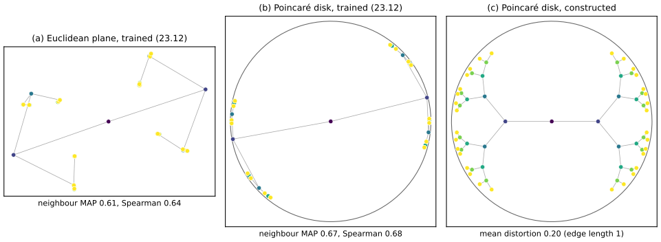
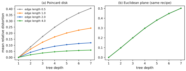
Figures and data. The book's nine figures are diagrams, reprinted drawings or molecule images; nothing in them is computed. Figures 23.1 and 23.6 are re-made with computed content (a grid against a real irregular graph; a tree embedded in the Euclidean plane and in the Poincaré disk), and Figures 23.S1 to 23.S8 are supplementary figures for the gaps. Figures 23.2, 23.3, 23.4, 23.5, 23.7, 23.8 and 23.9 (block diagrams, a transaction schema, molecule pictures) are not reproduced. Data: Zachary's karate-club graph (34 members, 78 ties, two factions) from networkx, two interleaved half-moons from scikit-learn, and simulated planted-partition graphs with Gaussian node features; the book supplies no data of its own. The book has no end-of-chapter exercises for this chapter, so the exercises section holds three supplementary ones. The ▶ Demo boxes open an interactive demonstration set to the case being discussed.
Main reference
K. P. Murphy, Probabilistic Machine Learning: An Introduction, MIT Press (2022), Chapter 23, pages 753–772 (book page: probml.github.io/pml-book/book1.html); the chapter is based on a survey by Chami, Abu-El-Haija, Perozzi, Ré and Murphy. Section, equation and figure numbers below refer to this book. The explanations, derivations, figures and code are my own.
Companion courses
Several pieces of this chapter are developed in full elsewhere on this site. These notes then give the statement and a short sketch and link to it.
- Foundations of Deep Learning (Bishop and Bishop): 13.1.3 permutation equivariance, 13.2.2 graph convolutional networks, 13.3.1 graph attention networks, 13.3.4 over-smoothing.
- Elements of Statistical Learning: 14.5.3 spectral clustering (the Laplacian eigenproblem of gap 23.1), 14.8 multidimensional scaling (gap 23.2) and 14.10 PageRank (random walks on a graph).
- Bayesian and Probabilistic Machine Learning (Bishop): 12.1 principal component analysis (the Eckart–Young step of gap 23.3) and 12.3 kernel PCA.
- Introduction to Statistical Learning: Chapter 12 on unsupervised learning (PCA and clustering).
What this chapter adds: the encoder/decoder language for graph methods, hyperbolic embeddings for hierarchies, the implicit-factorisation view of DeepWalk, label propagation as a harmonic function, and GNN variants (message passing, sampling, attention, contrastive learning).
The chapter at a glance
- 23.2 The loss \(\alpha\mathcal L_{\rm SUP}+\beta\mathcal L_{G,{\rm RECON}}+\gamma\mathcal L_{\rm REG}\) and its three ingredients: encoder, decoder, classifier.
- 23.3.2 Distance-based embeddings: classical MDS (gap 23.2) and Laplacian eigenmaps (gap 23.1).
- 23.3.3 Poincaré embeddings and their loss (gap 23.14, gap 23.15).
- 23.3.4 Matrix factorisation: Eckart–Young and the masked loss of graph factorisation (gap 23.3); GraRep (gap 23.4).
- 23.3.5 DeepWalk: the window distribution, the loss, and skip-gram as matrix factorisation (gap 23.5, gap 23.6, gap 23.7).
- 23.3.6 Label propagation and label spreading (gap 23.8).
- 23.4 GNNs: fixed point and implicit gradient (gap 23.9), message passing (gap 23.10), spectral convolutions and over-smoothing (gap 23.11), sampling (gap 23.12), attention (gap 23.13).
- 23.5 Graph auto-encoders and the variational bound (gap 23.16), deep graph infomax (gap 23.17).
Notation. \(\bm A\in\{0,1\}^{N\times N}\) is the adjacency matrix and \(\bm W\) a weighted version; \(\bm D=\diag(d_1,\dots,d_N)\) with \(d_i=\sum_jW_{ij}\) the degree matrix; \(\vol=\sum_id_i\); \(\bm L=\bm D-\bm W\) the (unnormalised) Laplacian; \(\bm P=\bm D^{-1}\bm W\) the random-walk transition matrix; \(\bm X\in\R^{N\times D}\) node features; \(\bm Z\in\R^{N\times L}\) the embedding with rows \(\bm z_i\). All graphs are undirected unless said otherwise.
Prerequisites. Chapter 7 (eigendecomposition, SVD, Eckart–Young), Chapter 8 (gradient methods), Chapter 6 (KL divergence) and, for the skip-gram section, the word-embedding material of Section 20.5.
23.1 Introduction
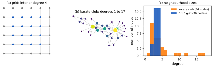
pp. 753–754 Graph-structured data comes with relations (edges) between the training samples (nodes): friendships, citations, bonds between atoms, links between web pages. An image is a very special graph, a grid in which every interior pixel has the same four neighbours in the same positions, so a convolution can reuse one filter everywhere. A general graph has no such alignment: neighbourhoods differ in size and have no natural ordering, so Euclidean convolutions do not apply directly (Figure 23.1). Graph representation learning maps nodes (or whole graphs) to low-dimensional vectors; the book separates unsupervised methods, which preserve graph structure, from supervised ones, which are trained for a prediction task, and transductive settings (one fixed graph, as in predicting attributes of users in a social network) from inductive ones (new graphs at test time, as in molecules). Non-Euclidean embedding spaces, notably hyperbolic space, are a third axis.
See also: permutation equivariance in Foundations of Deep Learning, the symmetry that replaces the grid's shift invariance.
23.2 Graph Embedding as an Encoder/Decoder Problem
pp. 754–756 Most methods fit one template, the graph encoder-decoder model. An encoder maps the weighted graph \(\bm W\) and optional features \(\bm X\) to embeddings, a decoder maps embeddings back to a matrix of pairwise scores, and (when labels exist) a classifier predicts labels from the embeddings: \[ \bm Z=\ENC(\bm W,\bm X;\bm\Theta_E),\tag{23.1} \] \[ \widehat{\bm W}=\DEC(\bm Z;\bm\Theta_D),\tag{23.2} \] \[ \hat{\bm y}^{S}=\DEC(\bm Z;\bm\Theta_S),\qquad S\in\{\mathcal N,\mathcal E,\mathcal G\}\ \text{(nodes, edges, graph)}.\tag{23.3} \] Training minimises a weighted sum of a supervised loss, a graph-reconstruction loss and a regulariser: \[ \mathcal L=\alpha\,\mathcal L^{S}_{\rm SUP}(\bm y^S,\hat{\bm y}^S;\bm\Theta)+\beta\,\mathcal L_{G,{\rm RECON}}(\bm W,\widehat{\bm W};\bm\Theta)+\gamma\,\mathcal L_{\rm REG}(\bm\Theta).\tag{23.4} \] Setting \(\alpha=0\) gives an unsupervised method. The rest of the chapter is a catalogue of choices of encoder (a table, a neural network), of the decoder (a distance, an inner product), of the target \(s(\bm W)\) and of the discrepancy \(d_1\) between \(s(\bm W)\) and \(\widehat{\bm W}\).
23.3 Shallow graph embeddings
p. 756 A shallow encoder is a look-up table: node \(i\) owns a free vector \(\bm z_i\in\R^L\) and \(\bm Z=\bm\Theta_E\in\R^{N\times L}\) is the parameter itself (23.5). The graph enters only through the loss. Such methods are transductive: a node absent at training time has no row in the table. The unsupervised case resembles PCA (Section 20.1) with a graph in place of a data matrix.
23.3.1 Unsupervised embeddings
p. 757 Two families are distinguished by the decoder. Distance-based methods take \(\widehat W_{ij}=d_2(\bm z_i,\bm z_j)\) and make connected nodes close. Outer-product methods take \(\widehat{\bm W}=\bm Z\bm Z^\T\) and make connected nodes have a large inner product. Both minimise \[ \mathcal L_{G,{\rm RECON}}(\bm W,\widehat{\bm W};\bm\Theta)=d_1\big(s(\bm W),\widehat{\bm W}\big),\tag{23.6} \] where \(s(\bm W)\) is a transformation of the graph (the matrix itself, a power, \(\mathbf 1-\bm W\), a matrix of shortest-path distances) and \(d_1\) a discrepancy between matrices, for instance the squared Frobenius norm.
23.3.2 Distance-based: Euclidean methods
pp. 757–758 Multi-dimensional scaling. Take \(s(\bm W)\) to be a matrix of dissimilarities (for instance hop distances) and \(\widehat W_{ij}=\|\bm z_i-\bm z_j\|\); the loss is the stress \[ d_1\big(s(\bm W),\widehat{\bm W}\big)=\sum_{i,j}\big(s(\bm W)_{ij}-\widehat W_{ij}\big)^2=\|s(\bm W)-\widehat{\bm W}\|_F^2.\tag{23.7} \] Minimising the stress needs iterative optimisation; classical MDS instead matches squared distances to inner products and is solved by one eigendecomposition (gap 23.2).
Laplacian eigenmaps. They solve \[ \min_{\bm Z\in\R^{N\times d}}\operatorname{tr}(\bm Z^\T\bm L\bm Z)\quad\text{s.t.}\quad\bm Z^\T\bm D\bm Z=\bm I,\ \ \bm Z^\T\bm D\mathbf 1=\bm 0,\tag{23.8} \] and since \(\operatorname{tr}(\bm Z^\T\bm L\bm Z)=\frac12\sum_{ij}W_{ij}\|\bm z_i-\bm z_j\|^2\), the objective is a reconstruction loss with \[ d_1\big(s(\bm W),\widehat{\bm W}\big)=\sum_{i,j}W_{ij}\widehat W_{ij},\qquad \widehat W_{ij}=\|\bm z_i-\bm z_j\|_2^2\tag{23.9, 23.10} \] (up to the factor \(\tfrac12\); the two constraints remove the scale and the constant eigenvector).
Filling the gap 23.1: the Laplacian quadratic form, and the eigenvector solution of (23.8) pp. 757–758, (23.8)–(23.10)
Derivation
The quadratic form. For symmetric \(\bm W\) and any \(\bm Z\) with rows \(\bm z_i\), \[ \sum_{i,j}W_{ij}\|\bm z_i-\bm z_j\|^2=\sum_{ij}W_{ij}\big(\|\bm z_i\|^2+\|\bm z_j\|^2-2\bm z_i^\T\bm z_j\big)=2\sum_id_i\|\bm z_i\|^2-2\sum_{ij}W_{ij}\bm z_i^\T\bm z_j=2\operatorname{tr}\big(\bm Z^\T(\bm D-\bm W)\bm Z\big), \] using \(\sum_jW_{ij}=d_i\). Hence \(\operatorname{tr}(\bm Z^\T\bm L\bm Z)=\frac12\sum_{ij}W_{ij}\|\bm z_i-\bm z_j\|^2\ge0\) when \(W_{ij}\ge0\): \(\bm L\) is positive semi-definite, and \(\bm L\mathbf 1=\bm 0\). If the graph is connected, \(\bm u^\T\bm L\bm u=0\) forces \(u_i=u_j\) along every edge, so the null space is spanned by \(\mathbf 1\) and \(0\) is a simple eigenvalue.
The solution of (23.8). Put \(\bm Y=\bm D^{1/2}\bm Z\). Then \(\bm Z^\T\bm D\bm Z=\bm Y^\T\bm Y=\bm I\), \(\bm Z^\T\bm D\mathbf 1=\bm Y^\T\bm D^{1/2}\mathbf 1\), and \(\operatorname{tr}(\bm Z^\T\bm L\bm Z)=\operatorname{tr}(\bm Y^\T\bm L_{\rm sym}\bm Y)\) with \(\bm L_{\rm sym}=\bm D^{-1/2}\bm L\bm D^{-1/2}=\bm I-\bm D^{-1/2}\bm W\bm D^{-1/2}\), a symmetric matrix with eigenvalues \(0=\lambda_1<\lambda_2\le\dots\le\lambda_N\) and eigenvector \(\bm D^{1/2}\mathbf 1\) (normalised) for \(\lambda_1\) (because \(\bm L_{\rm sym}\bm D^{1/2}\mathbf 1=\bm D^{-1/2}\bm L\mathbf 1=\bm0\)). The second constraint says that the columns of \(\bm Y\) are orthogonal to that eigenvector. By Ky Fan's theorem (the sum of the \(d\) smallest eigenvalues of a symmetric matrix is the minimum of \(\operatorname{tr}(\bm Y^\T\bm M\bm Y)\) over \(\bm Y^\T\bm Y=\bm I\), attained by the corresponding eigenvectors; restricted to the orthogonal complement of the bottom eigenvector the same holds for the remaining spectrum), the minimum is \(\lambda_2+\dots+\lambda_{d+1}\), attained by the eigenvectors \(\bm v_2,\dots,\bm v_{d+1}\) of \(\bm L_{\rm sym}\), i.e. \(\bm Z=\bm D^{-1/2}[\bm v_2,\dots,\bm v_{d+1}]\). Equivalently, the columns of \(\bm Z\) solve the generalised eigenproblem \(\bm L\bm z=\lambda\bm D\bm z\), and \(\bm D^{-1/2}\bm W\bm D^{-1/2}\) has eigenvalues \(1-\lambda_k\). Numerical confirmation. On the karate-club graph the smallest non-zero generalised eigenvalues are \(\lambda_2=0.1323\) and \(\lambda_3=0.2870\); the objective at the eigenvector solution equals \(\lambda_2+\lambda_3\), 300 random feasible matrices never do better, and the sign of the first coordinate (the Fiedler vector) places 32 of the 34 members on the correct side of the factional split. \(\square\)
Remark. The same eigenvectors, followed by k-means, are spectral clustering (companion course, ESL 14.5.3).
Filling the gap 23.2: classical MDS and its relation to PCA p. 757, (23.7), Section 20.4.4
Derivation
Suppose points \(\bm z_i\in\R^d\) have squared distances \(\Delta_{ij}^2=\|\bm z_i-\bm z_j\|^2=\|\bm z_i\|^2+\|\bm z_j\|^2-2\bm z_i^\T\bm z_j\). Let \(\bm J=\bm I-\frac1N\mathbf 1\mathbf 1^\T\) be the centring matrix and \(\bm\Delta^{(2)}=(\Delta_{ij}^2)\). Centring both sides, \(\bm J(\bm a\mathbf 1^\T)\bm J=\bm 0\) and \(\bm J(\mathbf 1\bm a^\T)\bm J=\bm0\) for any vector \(\bm a\) (here \(a_i=\|\bm z_i\|^2\)), so \[ -\tfrac12\bm J\bm\Delta^{(2)}\bm J=\bm J\bm Z\bm Z^\T\bm J=\tilde{\bm Z}\tilde{\bm Z}^\T,\qquad\tilde{\bm Z}=\bm J\bm Z\ \text{(the centred coordinates)}.\] Thus the double-centred squared-distance matrix \(\bm B\) is a Gram matrix of rank at most \(d\), positive semi-definite. If \(\tilde{\bm Z}=\bm U\bm S\bm V^\T\) is its SVD, then \(\bm B=\bm U\bm S^2\bm U^\T\), so an eigendecomposition \(\bm B=\bm Q\bm\Lambda\bm Q^\T\) returns the centred configuration as \(\bm Q\bm\Lambda^{1/2}=\bm U\bm S\), the principal-component scores of the data (the right rotation \(\bm V\) is lost: distances do not see rotations). For a general dissimilarity matrix (as for hop distances, which need not be Euclidean) \(\bm B\) may have negative eigenvalues; classical MDS keeps the \(d\) largest positive ones and sets \(\bm Z=\bm Q_{1:d}\bm\Lambda_{1:d}^{1/2}\), which by Eckart–Young (gap 23.3) is the best rank-\(d\) PSD approximation of \(\bm B\) in Frobenius norm. This is a different objective from the stress (23.7), which compares distances, not squared distances, and is minimised iteratively. Numerical confirmation. For 40 random points in \(\R^3\), MDS with \(d=3\) reproduces all pairwise distances to \(10^{-8}\) and its coordinates equal the PCA scores up to signs. \(\square\)
See also: multidimensional scaling and spectral clustering in the ESL companion course.
23.3.3 Distance-based: non-Euclidean methods
p. 758 Trees and other hierarchies have exponentially many nodes at depth \(r\); a Euclidean ball of radius \(r\) in \(\R^L\) has volume only \(\propto r^L\), so large trees cannot be embedded in a low-dimensional Euclidean space without distorting distances (gap 23.14 gives a counting proof). The hyperbolic plane has circumference growing like \(e^r\) and embeds trees almost isometrically. Nickel and Kiela use the Poincaré ball \(\{\bm x:\|\bm x\|<1\}\) with the distance \[ d_{\rm Poincar\acute e}(\bm z_i,\bm z_j)=\arcosh\!\Big(1+2\,\frac{\|\bm z_i-\bm z_j\|_2^2}{(1-\|\bm z_i\|_2^2)(1-\|\bm z_j\|_2^2)}\Big),\tag{23.11} \] as the decoder, and learn embeddings that bring connected nodes together and push unconnected ones apart through a softmax-type loss with negative sampling, \[ d_1(\bm W,\widehat{\bm W})=\sum_{i,j}W_{ij}\log\frac{e^{-\widehat W_{ij}}}{\sum_{k:W_{ik}=0}e^{-\widehat W_{ik}}}.\tag{23.12} \] Because the parameters live on a manifold, optimisation uses Riemannian SGD (gap 23.15). Other models use the Lorentz (hyperboloid) model, which is numerically more stable, mixed-curvature product spaces, or skip-gram losses with hyperbolic inner products.
Filling the gap 23.14: the Poincaré distance, its isometries, and why trees need hyperbolic room p. 758, (23.11)
Derivation
Where (23.11) comes from. The Poincaré ball is the open unit ball with the Riemannian metric \(\d s^2=\frac{4\|\d\bm x\|^2}{(1-\|\bm x\|^2)^2}\), conformal to the Euclidean one and blowing up at the rim. Along a ray from the origin, \(r=\|\bm x\|\), the length is \(\int_0^r\frac{2\,\d\rho}{1-\rho^2}=\ln\frac{1+r}{1-r}=2\artanh r\); this is the geodesic from the origin (a straight segment by symmetry), so \[ d(\bm 0,\bm x)=2\artanh\|\bm x\|.\] Put \(\bm y=\bm 0\) in (23.11): \(\arcosh\big(1+\frac{2r^2}{1-r^2}\big)=\arcosh\frac{1+r^2}{1-r^2}\), and since \(\cosh(2u)=\frac{1+\tanh^2u}{1-\tanh^2u}\), this equals \(2\artanh r\), as it should. For general points one uses that Möbius transformations of the ball (in the plane, \(z\mapsto\frac{z+p}{1+\bar pz}\) in complex notation, which moves \(0\) to \(p\)) are isometries of the metric and that the expression \(\frac{\|\bm x-\bm y\|^2}{(1-\|\bm x\|^2)(1-\|\bm y\|^2)}\) is invariant under them: composing the translation that moves \(\bm x\) to the origin with the formula above gives (23.11). Numerical confirmation. The integral of the metric along a radius equals \(2\artanh r\); translations of the disk leave all pairwise distances of random points unchanged to \(10^{-9}\); the triangle inequality holds on 30 random points.
Volume growth. In the hyperbolic plane a circle of radius \(r\) has circumference \(2\pi\sinh r\sim\pi e^r\), the same exponential rate at which a binary tree has \(2^r\) nodes at depth \(r\) (a complete binary tree has exactly \(2^{r+1}-1\) nodes within \(r\) edges of its root). In \(\R^L\) a ball of radius \(\rho\) has volume \(\propto\rho^L\).
Counting argument: trees are not Euclidean. Suppose the complete binary tree of depth \(h\) were mapped to \(\R^L\) by \(f\) with \(s\,d_T(u,v)\le\|f(u)-f(v)\|\le s\,c\,d_T(u,v)\) (distortion \(c\)), where \(d_T\) is the number of edges between \(u\) and \(v\). The \(2^h\) leaves are at pairwise tree distance at least \(2\), so their images are \(2s\)-separated; they all lie within \(s\,c\,h\) of the image of the root. Balls of radius \(s\) around the images are disjoint and lie in a ball of radius \(s(ch+1)\), so by comparing volumes \(2^h\le(ch+1)^L\), i.e. \(c\ge(2^{h/L}-1)/h\), which tends to infinity with \(h\) for fixed \(L\). In contrast, the hyperbolic plane admits embeddings of every tree with distortion arbitrarily close to 1 (Sarkar, 2011): place every child at hyperbolic distance \(\tau\) from its parent, spread in equal angles around the parent, and let \(\tau\) grow. Numerical confirmation. This construction gives the mean relative distortion of a depth-6 binary tree as 0.225, 0.114, 0.076, 0.057 for \(\tau=1,2,3,4\) (Figure 23.S8), every edge having hyperbolic length exactly \(\tau\), while the same recipe in the Euclidean plane has mean distortion 0.45 and worst distortion 1 at \(\tau=2\) (nodes collide). The price of the accuracy is a rim: points are at Euclidean radius \(\tanh(\tau k/2)\) at depth \(k\), exponentially close to 1. \(\square\)
Filling the gap 23.15: the loss (23.12) and Riemannian SGD p. 758, (23.12)
Derivation
The loss. For a related pair \((i,j)\) let \(\mathcal N(i,j)\) contain \(j\) and a sample of nodes not related to \(i\). The loss is the negative log-likelihood of picking \(j\) among them by a softmax of negative distances: \[ \ell_{ij}=-\log\frac{e^{-d(\bm z_i,\bm z_j)}}{\sum_{k\in\mathcal N(i,j)}e^{-d(\bm z_i,\bm z_k)}} .\] As printed, (23.12) is the log of this probability summed over edges, which is to be maximised; the minimised loss carries the opposite sign (see the notes on the book). Negative sampling replaces the sum over all non-neighbours by a small random subset.
Riemannian gradient. At a point \(\bm x\) of the ball the metric tensor is \(g_{\bm x}=\lambda_{\bm x}^2\bm I\) with \(\lambda_{\bm x}=\frac{2}{1-\|\bm x\|^2}\). The steepest-descent direction of a function \(f\) on a Riemannian manifold is \(-g_{\bm x}^{-1}\nabla_{\rm E}f\) (the direction \(\bm v\) minimising the first-order change \(\langle\nabla_{\rm E}f,\bm v\rangle\) subject to \(\|\bm v\|_{g}=1\)), so \[ \nabla_{\rm R}f(\bm x)=\frac{(1-\|\bm x\|^2)^2}{4}\nabla_{\rm E}f(\bm x),\qquad \bm x\leftarrow\operatorname{proj}\big(\bm x-\eta\,\nabla_{\rm R}f(\bm x)\big),\] where \(\operatorname{proj}\) pulls points that leave the ball back to just inside the rim (Nickel and Kiela use the retraction \(\bm x\mapsto\bm x-\eta\nabla_{\rm R}f\) followed by projection onto \(\|\bm x\|\le1-\varepsilon\)). The factor shrinks the step near the rim, where the metric is large. The Euclidean gradient of \(d\) is obtained by differentiating (23.11) (here by automatic differentiation). Numerical confirmation. The automatic-differentiation gradient of the Poincaré distance agrees with finite differences to \(10^{-8}\). Trained for 100 epochs on the 63-node binary tree in two dimensions, the Poincaré embedding ranks the tree neighbours of a node better than the Euclidean embedding trained with the same loss (mean average precision 0.67 against 0.61). \(\square\)
23.3.4 Outer product-based: Matrix factorization
pp. 758–759 Matrix-factorisation methods take the decoder \(\widehat{\bm W}=\bm Z\bm Z^\T\) (23.13) and fit it to a similarity matrix \(s(\bm W)\) (the adjacency matrix, the Laplacian, Katz, common-neighbour or Adamic–Adar scores) by minimising \(\|s(\bm W)-\widehat{\bm W}\|_F^2\). If the best rank-\(L\) approximation is wanted and \(s(\bm W)\) is symmetric, the answer is given by the leading eigenpairs (gap 23.3). Graph factorisation (Ahmed et al.) sums only over the existing edges, \[ \mathcal L_{G,{\rm RECON}}=\|\bm A\odot(\bm W-\widehat{\bm W})\|_F^2=\sum_{(i,j)\in\mathcal E}(W_{ij}-\widehat W_{ij})^2,\tag{23.14} \] which costs \(O(M)\) per pass for \(M\) edges. GraRep learns a source and a target embedding to handle directed graphs and uses powers to preserve \(k\)-hop neighbourhoods: \[ \widehat{\bm W}^{(k)}=\bm Z^{(k),s}\bm Z^{(k),t\,\T},\qquad\mathcal L=\big\|\bm D^{-k}\bm W^{k}-\widehat{\bm W}^{(k)}\big\|_F^2,\quad 1\le k\le K,\tag{23.15, 23.16} \] then concatenates the \(K\) embeddings. The powers become dense, so it does not scale; implicit factorisation of the skip-gram methods avoids this (Section 23.3.5).
Filling the gap 23.3: the best low-rank factorisation (Eckart–Young), and the masked loss (23.14) pp. 758–759, (23.13), (23.14)
Derivation
Claim. Let \(\bm S\) be real symmetric with eigenvalues \(\mu_1\ge\dots\ge\mu_N\) and orthonormal eigenvectors \(\bm q_k\). Among real \(\bm Z\in\R^{N\times L}\), \(\|\bm S-\bm Z\bm Z^\T\|_F^2\) is minimised by \(\bm Z=[\sqrt{\mu_1}\bm q_1,\dots,\sqrt{\mu_L}\bm q_L]\) when \(\mu_L\ge0\), with minimum \(\sum_{k>L}\mu_k^2\). If \(\bm S\) has negative eigenvalues the minimum over real \(\bm Z\) is \(\sum_{\mu_k<0}\mu_k^2+\sum_{k>L,\mu_k\ge0}\mu_k^2\) (\(\bm Z\bm Z^\T\) is PSD, so negative eigenvalues of \(\bm S\) cannot be matched), attained with the positive eigenvalues only.
Proof. Write \(\bm S=\bm Q\bm M\bm Q^\T\), and \(\bm T=\bm Q^\T\bm Z\bm Z^\T\bm Q\); since the Frobenius norm is invariant under orthogonal conjugation, \(\|\bm S-\bm Z\bm Z^\T\|_F^2=\|\bm M-\bm T\|_F^2=\sum_k(\mu_k-T_{kk})^2+\sum_{k\ne l}T_{kl}^2\). \(\bm T\) is PSD of rank \(\le L\). Rather than diagonalise \(\bm T\), compare in the eigenbasis directly. Write \(\bm M=\bm M_+-\bm M_-\) with \(\bm M_\pm\succeq0\) the positive and negative parts. For PSD \(\bm T\), \(\langle\bm M_-,\bm T\rangle\ge0\), so \(\langle\bm M,\bm T\rangle\le\langle\bm M_+,\bm T\rangle\) and \[ \|\bm M-\bm T\|_F^2=\|\bm M\|_F^2-2\langle\bm M,\bm T\rangle+\|\bm T\|_F^2\ \ge\ \|\bm M_+-\bm T\|_F^2+\|\bm M_-\|_F^2 .\] By the Eckart–Young–Mirsky theorem (for any matrix \(\bm R\) of rank \(\le L\), \(\|\bm M_+-\bm R\|_F^2\ge\sum_{k>L}\sigma_k(\bm M_+)^2\), a consequence of Weyl's inequality \(\sigma_{k+L}(\bm M_+)\le\sigma_k(\bm M_+-\bm R)\)), the first term is at least the sum of the squared dropped positive eigenvalues, and the truncated eigendecomposition of \(\bm M_+\) is PSD, of rank \(\le L\), and attains it while making the inequality \(\langle\bm M_-,\bm T\rangle=0\) an equality. So the minimum is \(\sum_{\mu_k<0}\mu_k^2+\sum_{k>L,\mu_k>0}\mu_k^2\), the claim; for PSD \(\bm S\) it is \(\sum_{k>L}\mu_k^2\). \(\square\)
Numerical confirmation. For a random PSD \(30\times30\) matrix the error of the rank-5 factorisation equals the root of the sum of the squared dropped eigenvalues; for an indefinite \(12\times12\) matrix the squared error equals the sum of the squared negative eigenvalues plus the squared dropped positive ones, and a numerical minimiser from six random starts does not beat it (59.6548 both).
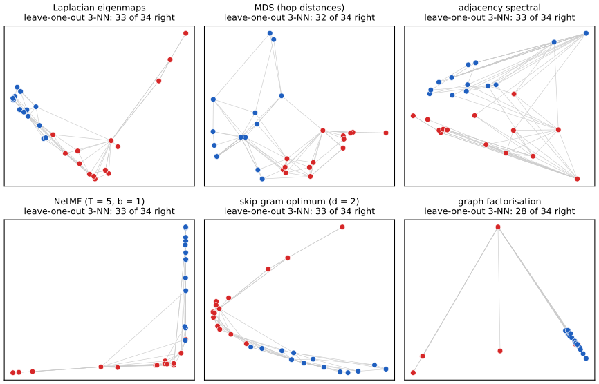
The masked loss. \(\bm A\odot(\bm W-\widehat{\bm W})\) has entries \(A_{ij}(W_{ij}-\widehat W_{ij})\), and \(A_{ij}^2=A_{ij}\) for a binary \(\bm A\), so \(\|\bm A\odot(\bm W-\widehat{\bm W})\|_F^2=\sum_{ij}A_{ij}(W_{ij}-\widehat W_{ij})^2\), a sum over the directed edges only (twice the sum over undirected edges). Gradient descent on it touches only \(M\) terms per step, giving the \(O(M)\) cost. The price is that non-edges impose nothing, so the loss is also minimised by embeddings that place unconnected nodes close together. On the karate club, graph factorisation in two dimensions fits the 156 directed edges to a mean absolute residual below 0.002 yet separates the factions only on 28 of 34 members by nearest neighbours (Figure 23.S1). \(\square\)
Filling the gap 23.4: what GraRep factorises p. 759, (23.15), (23.16)
Derivation
The aim of GraRep is to capture \(k\)-step proximity, which is encoded by the \(k\)-step transition matrix of the random walk, \(\bm P^k=(\bm D^{-1}\bm W)^k\), whose \((i,j)\) entry is the probability of being at \(j\) after \(k\) steps from \(i\) (Chapman–Kolmogorov: \(\bm P^{k}=\bm P\bm P^{k-1}\)). It is row-stochastic: \(\bm P\mathbf 1=\mathbf 1\Rightarrow\bm P^k\mathbf 1=\mathbf 1\). The matrix printed in (23.16), \(\bm D^{-k}\bm W^k\), is a different object: for \(k=2\), \((\bm D^{-2}\bm W^2)_{ij}=\frac1{d_i^2}\sum_lW_{il}W_{lj}\) whereas \((\bm P^2)_{ij}=\frac1{d_i}\sum_l\frac{W_{il}W_{lj}}{d_l}\); they coincide only if all degrees on the paths are equal (for instance regular graphs), and \(\bm D^{-2}\bm W^2\) is not row-stochastic in general. The intended target is therefore \(\bm P^k\). Numerical confirmation. On the karate club, \(\bm P^2\) has all row sums equal to 1, while \(\bm D^{-2}\bm A^2\) differs from it by up to 0.94 in a single entry and its row sums differ from 1. (GraRep itself factorises a logarithm of \(\bm P^k\) normalised by the column sums, in the original paper; the book's version drops this.) The best rank-\(L\) factorisation of an asymmetric target \(\bm T\) in Frobenius norm is the truncated SVD \(\bm T\approx\bm U_L\bm S_L\bm V_L^\T\), giving \(\bm Z^{s}=\bm U_L\bm S_L^{1/2}\), \(\bm Z^t=\bm V_L\bm S_L^{1/2}\) (Eckart–Young, gap 23.3). \(\square\)
23.3.5 Outer product-based: Skip-gram methods
pp. 759–760 Skip-gram word embeddings predict the words around a target word. DeepWalk applies this to graphs: simulate truncated random walks (each step moves to a neighbour chosen uniformly), treat each walk as a sentence, and train embeddings to predict the context nodes (those within a window of the centre) from the centre node, with the decoder \(\widehat{\bm W}=\bm Z\bm Z^\T\); in practice two vectors per node are used, a centre vector and a context vector, \(\widehat{\bm W}=\bm Z_{\rm out}\bm Z_{\rm in}^\T\). In the GraphEDM language the target is the expected window-averaged transition matrix, \[ s(\bm W)=\E_{q}\big[(\bm D^{-1}\bm W)^q\big],\qquad q\sim P(Q)=\mathrm{Cat}\big([1,\dots,T_{\max}]\big),\tag{23.17} \] and the loss, with the partition function approximated by hierarchical softmax or negative sampling (Section 20.5.2), is \[ \mathcal L_{G,{\rm RECON}}(\bm W,\widehat{\bm W};\bm\Theta)=\log\mathcal Z(\bm Z)-\sum_{v_i,v_j}s(\bm W)_{ij}\widehat W_{ij},\qquad\mathcal Z(\bm Z)=\prod_i\sum_j\exp(\widehat W_{ij}).\tag{23.18} \] Skip-gram is an implicit matrix factorisation (Levy and Goldberg; Qiu et al., NetMF), which links the section to Section 23.3.4 (gap 23.7). Figure 23.4 of the book (the pipeline of random-walk methods: walks, then a sequence model) is a diagram and is not reproduced.
Filling the gap 23.5: the window distribution in (23.17) p. 760, (23.17)
Derivation
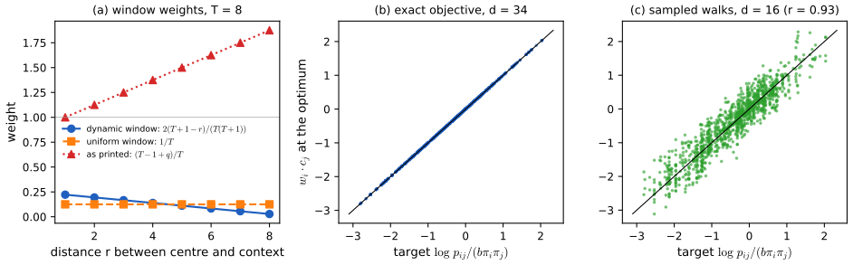
What the walk produces. Start a walk from a node and let it run; if it is stationary (started from \(\pi_i=d_i/\vol\)), the pair (node at position \(t\), node at position \(t+r\)) has the joint law \(\pi_i(\bm P^r)_{ij}\), because the walk is a Markov chain with transition matrix \(\bm P\); and it is symmetric in \((i,j)\) for undirected graphs (reversibility, \(\pi_iP_{ij}=\pi_jP_{ji}\)). A skip-gram implementation then chooses which pairs to use. With the uniform window of size \(T\), all offsets \(r=1,\dots,T\) are used equally, so a random (centre, context) pair has distance \(r\) with probability \(\omega_r=1/T\). With the word2vec dynamic window, the window size \(b\) is first drawn uniformly from \(\{1,\dots,T\}\) at each centre and every offset \(r\le b\) is used; a pair at offset \(r\) is therefore used with probability \(\Pr(b\ge r)=\frac{T-r+1}{T}\), and, normalised to a distribution over offsets, \[ \omega_r=\frac{T+1-r}{\sum_{u=1}^{T}(T+1-u)}=\frac{2(T+1-r)}{T(T+1)},\qquad r=1,\dots,T.\] In both cases the pair distribution is \(p_{ij}=\sum_{r=1}^T\omega_r\pi_i(\bm P^r)_{ij}\), i.e. in matrix form \(\bm\Pi\,\E_{q\sim\omega}[\bm P^q]\) with \(\bm\Pi=\diag(\pi)\): this is (23.17) with \(P(Q=q)=\omega_q\), which is a probability distribution on \(\{1,\dots,T_{\max}\}\) that does not increase with \(q\). The formula \(P(Q=q)=\frac{T_{\max}-1+q}{T_{\max}}\) printed in the book is not such a distribution (see the notes on the book): for \(T_{\max}=5\) the values sum to 7. Numerical confirmation. Simulating the dynamic window 200,000 times reproduces \(\omega_r\) to \(0.003\); 51,000 walks of length 35 (1500 rounds over the 34 starting nodes) on the karate club with the dynamic window give pair frequencies within total-variation distance 0.008 of \(\sum_r\omega_r\pi_i(\bm P^r)_{ij}\); the pair distribution sums to 1 and has both marginals \(\pi\). \(\square\)
Filling the gap 23.6: the loss (23.18) as a cross entropy p. 760, (23.18)
Derivation
Let \(p_{ij}\) be the pair distribution of the previous gap, \(\sum_{ij}p_{ij}=1\), with row sums \(\pi_i\). A skip-gram model predicts the context \(j\) from the centre \(i\) by the softmax \(q_\theta(j\given i)=\exp(\widehat W_{ij})/\sum_{k}\exp(\widehat W_{ik})\). The expected negative log-likelihood per pair is \[ -\sum_{ij}p_{ij}\log q_\theta(j\given i)=-\sum_{ij}p_{ij}\widehat W_{ij}+\sum_i\pi_i\log\sum_k e^{\widehat W_{ik}}.\] If the target is normalised by rows, \(s(\bm W)_{ij}=p_{ij}/\pi_i=\E_q[(\bm P^q)_{ij}]\) (each row sums to 1), and if all centres are weighted equally (\(\pi_i\) replaced by \(1\)), the loss becomes \(\sum_i\log\sum_ke^{\widehat W_{ik}}-\sum_{ij}s_{ij}\widehat W_{ij}=\log\mathcal Z-\sum_{ij}s_{ij}\widehat W_{ij}\) with \(\mathcal Z=\prod_i\sum_je^{\widehat W_{ij}}\), exactly (23.18); the rows of \(s\) summing to one is what makes every row's log-partition term appear with weight 1. (With the non-uniform weights \(\pi_i\) of true walk statistics the log-partition terms carry a factor \(\pi_i\).) Each row is a cross entropy, minimised when \(q_\theta(\cdot\given i)\) equals the row of \(s\): the softmax of the scores reproduces the \(q\)-step transition probabilities, and the minimum of the loss is the sum of the row entropies. Computing the denominators costs \(O(N)\) per centre, hence hierarchical softmax or negative sampling (gap 23.7). \(\square\)
Filling the gap 23.7: skip-gram with negative sampling is an implicit matrix factorisation p. 760, (23.18), [LG14], [Qiu+18]
Derivation
Setting. Skip-gram with negative sampling (SGNS) draws a pair \((i,j)\) from \(p_{ij}\) and \(b\) negative contexts \(k\) independently from the context marginal \(\pi_k\), and minimises \[ \mathcal L(\bm W,\bm C)=-\sum_{ij}\Big[p_{ij}\log\sigma(x_{ij})+b\,\pi_i\pi_j\log\sigma(-x_{ij})\Big],\qquad x_{ij}=\bm w_i^\T\bm c_j\] in expectation (centre vector \(\bm w_i\), context vector \(\bm c_j\)), since a given ordered pair \((i,j)\) appears as a positive with probability \(p_{ij}\) and as a negative with probability \(b\,\pi_i\pi_j\) per sample.
Result. If the dimension is large enough that \(x_{ij}\) can be set freely, the minimiser is \[ \bm w_i^\T\bm c_j=\log\frac{p_{ij}}{b\,\pi_i\pi_j}.\] Proof. \(\mathcal L\) separates over pairs: for each \((i,j)\) minimise \(f(x)=-p\log\sigma(x)-q\log\sigma(-x)\) with \(p=p_{ij}\), \(q=b\pi_i\pi_j\). Its derivative is \(f'(x)=-p\,\sigma(-x)+q\,\sigma(x)\), which is zero iff \(\frac{\sigma(x)}{\sigma(-x)}=e^{x}=\frac pq\); and \(f''=(p+q)\sigma(x)\sigma(-x)>0\), so the stationary point \(x=\log(p/q)\) is the global minimum. \(\square\)
Consequence (NetMF). With the uniform window, \(p_{ij}=\frac1T\sum_{r\le T}\pi_i(\bm P^r)_{ij}\), \(\pi_i=d_i/\vol\), so \[ \frac{p_{ij}}{b\,\pi_i\pi_j}=\Big[\frac{\vol}{bT}\sum_{r=1}^T\bm P^r\bm D^{-1}\Big]_{ij},\] and the SGNS solution is \(\bm W\bm C^\T=\log\bm M\) with \(\bm M=\frac{\vol}{bT}\sum_r\bm P^r\bm D^{-1}\) (symmetric for undirected graphs, since \(\bm P^r\bm D^{-1}=\bm D^{-1}\bm W(\bm D^{-1}\bm W)^{r-1}\bm D^{-1}\) is a product of the symmetric form \(\bm D^{-1/2}(\bm D^{-1/2}\bm W\bm D^{-1/2})^r\bm D^{-1/2}\)). When some entries of \(\bm M\) are below 1 the log is negative or minus infinity (pairs never seen together); NetMF therefore factorises the clipped matrix \(\log\max(\bm M,1)\) at rank \(L\) by the eigendecomposition of gap 23.3. For the dynamic window replace \(1/T\) by \(\omega_r\). Skip-gram methods are thus matrix factorisation with the decoder \(\bm Z\bm Z^\T\) and a specific data-dependent target, which explains why \(\bm P^r\) need not be formed in the training loop (the factorisation is implicit) and why larger \(b\) shifts the target down by \(\log b\). Numerical confirmation. On the karate club with a window of 10 and \(b=1\), minimising the exact expected SGNS loss with \(L=34\) gives inner products equal to the closed-form target to \(1.1\times10^{-4}\) (Figure 23.S2b); the gradient formula agrees with finite differences; a DeepWalk implementation trained by SGD on 3400 sampled walks with \(L=16\) gives inner products correlated 0.93 with the target (Figure 23.S2c). For \(b=1\) and \(T=5\) 384 of the 1156 entries of \(\bm M\) exceed 1, for \(b=5\) only 17 do. \(\square\)
See also: PageRank (ESL 14.10): the same random walk, summarised by its stationary distribution \(\pi\).
23.3.6 Supervised embeddings
p. 761 Learning unsupervised embeddings and then training a classifier on them is not ideal: the embedding need not preserve what matters for the task. Methods that combine the two steps keep the embedding shallow and use a few labels.
23.3.6.1 Label propagation
p. 761 In label propagation (Zhu and Ghahramani) the embedding is the label distribution itself, \(\hat{\bm y}^{\mathcal N}=\bm Z\), and the graph regulariser asks neighbouring nodes to have similar labels, \[ \mathcal L_{G,{\rm RECON}}=\sum_{i,j}W_{ij}\|\hat{\bm y}_i^{\mathcal N}-\hat{\bm y}_j^{\mathcal N}\|_2^2,\tag{23.19} \] minimised over functions that equal the true labels on the labelled nodes \(V_L\) by an iteration that replaces each unlabelled node's label distribution by the weighted average of its neighbours'. Label spreading (Zhou et al.) minimises the degree-normalised version \[ \mathcal L_{G,{\rm RECON}}=\sum_{i,j}W_{ij}\Big\|\frac{\hat{\bm y}_i^{\mathcal N}}{\sqrt{D_i}}-\frac{\hat{\bm y}_j^{\mathcal N}}{\sqrt{D_j}}\Big\|_2^2,\tag{23.20} \] and in both the supervised loss is the squared distance to the one-hot labels on the labelled nodes, \[ \mathcal L^{\mathcal N}_{\rm SUP}(\bm y^{\mathcal N},\hat{\bm y}^{\mathcal N})=\sum_{i:v_i\in V_L}\|\bm y_i^{\mathcal N}-\hat{\bm y}_i^{\mathcal N}\|_2^2.\tag{23.21} \] The methods work well on graphs in which proximity correlates positively with label similarity (homophily).
Filling the gap 23.8: the harmonic solution of label propagation, and the closed form of label spreading p. 761, (23.19)–(23.21)
Derivation
Harmonic solution. Split the nodes into labelled \(L\) and unlabelled \(U\) and fix \(\bm f_L=\bm Y_L\) (one column per class). The energy \(E(\bm f)=\frac12\sum_{ij}W_{ij}(f_i-f_j)^2=\bm f^\T\bm L\bm f\) (gap 23.1) is, in block form, \[ E=\bm f_L^\T\bm L_{LL}\bm f_L+2\bm f_U^\T\bm L_{UL}\bm f_L+\bm f_U^\T\bm L_{UU}\bm f_U .\] Its gradient in \(\bm f_U\) is \(2(\bm L_{UL}\bm f_L+\bm L_{UU}\bm f_U)\). \(\bm L_{UU}=\bm D_{UU}-\bm W_{UU}\) is positive definite if every connected component contains a labelled node (it is PSD as a principal submatrix of \(\bm L\), and \(\bm u^\T\bm L_{UU}\bm u=0\) would force \(\bm u\oplus\bm 0\) to be constant on each component, hence zero). Therefore \(E\) is strictly convex in \(\bm f_U\) with the unique minimiser \[ \bm f_U=-\bm L_{UU}^{-1}\bm L_{UL}\bm f_L=(\bm D_{UU}-\bm W_{UU})^{-1}\bm W_{UL}\bm f_L=(\bm I-\bm P_{UU})^{-1}\bm P_{UL}\bm f_L ,\] using \(\bm L_{UL}=-\bm W_{UL}\). This says \(f_i=\sum_jP_{ij}f_j\) for \(i\in U\): each unlabelled value is the weighted average of its neighbours' (the function is harmonic).
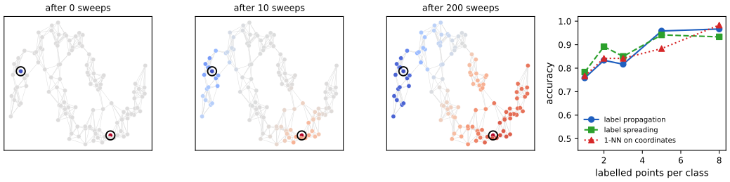
Iteration. The update \(\bm f_U^{t+1}=\bm P_{UU}\bm f_U^t+\bm P_{UL}\bm f_L\) is an affine map with linear part \(\bm P_{UU}\), a sub-stochastic matrix with spectral radius \(<1\) when every component has a labelled node (the walk leaves \(U\) with positive probability from every state). Hence \(\sum_t\bm P_{UU}^t=(\bm I-\bm P_{UU})^{-1}\) converges and the iteration converges geometrically to the fixed point above, which is the harmonic solution, from any start. The rate is the spectral radius of \(\bm P_{UU}\), close to 1 when labelled nodes are far, so convergence can be slow (on 120 points with 3 labels per class, 1455 sweeps are needed for \(10^{-13}\)).
Random-walk meaning. Let \(h_i\) be the probability that a random walk started at \(i\in U\) is first absorbed in a class-1 labelled node. Conditioning on the first step, \(h_i=\sum_jP_{ij}h_j\) with \(h=1\) on class-1 labelled nodes and \(0\) on the others: the same equations, so \(f_i=h_i\). Since \(h_i\in[0,1]\) and the class probabilities sum to 1 (maximum principle), the rows of the solution are probability vectors. Numerical confirmation. On two half-moons the iteration converges to the closed form; every unlabelled value is a neighbour average to \(10^{-10}\); 100 random perturbations of the unlabelled values all increase the energy; the absorption frequency of 4000 simulated walks (0.145) matches the harmonic value (0.140); on a path of 9 nodes with the ends labelled 0 and 1 the solution is the linear interpolation \(i/8\).
Label spreading. Add a fit term to the normalised energy: \(Q(\bm F)=\frac12\sum_{ij}W_{ij}\|\bm F_i/\sqrt{d_i}-\bm F_j/\sqrt{d_j}\|^2+\frac\mu2\|\bm F-\bm Y\|_F^2=\operatorname{tr}\bm F^\T(\bm I-\bm S)\bm F+\frac\mu2\|\bm F-\bm Y\|_F^2\) with \(\bm S=\bm D^{-1/2}\bm W\bm D^{-1/2}\) (by the computation of gap 23.1 with \(\bm F_i/\sqrt{d_i}\) in place of \(\bm z_i\)). Setting the gradient to zero, \(2(\bm I-\bm S)\bm F+\mu(\bm F-\bm Y)=\bm 0\), gives \(\big((2+\mu)\bm I-2\bm S\big)\bm F=\mu\bm Y\); with \(\alpha=\frac2{2+\mu}\) this is \(\bm F=(1-\alpha)(\bm I-\alpha\bm S)^{-1}\bm Y\). (Rescaling the energy rescales \(\mu\): with \(\frac14\sum_{ij}W_{ij}\|\cdot\|^2+\frac\mu2\|\bm F-\bm Y\|_F^2\) one gets \(\alpha=1/(1+\mu)\).) The matrix \(\bm I-\alpha\bm S\) is invertible since the eigenvalues of \(\bm S\) lie in \([-1,1]\) (gap 23.11), and the iteration \(\bm F\leftarrow\alpha\bm S\bm F+(1-\alpha)\bm Y\) converges to it because \(\|\alpha\bm S\|_2\le\alpha<1\): the series \((1-\alpha)\sum_t(\alpha\bm S)^t\bm Y\). Unlike label propagation, the labelled nodes are not clamped: \(\alpha\) trades smoothness against fidelity to the given labels. Numerical confirmation. Closed form and iteration agree to \(10^{-9}\) and the gradient of the energy vanishes at the closed form (with \(\alpha=0.9\)). \(\square\)
See also: spectral clustering (ESL), where the same Laplacian appears without labels.
23.4 Graph Neural Networks
p. 762 Shallow embeddings are free tables. A graph neural network replaces the table by an encoder \(\bm Z=\ENC(\bm X,\bm W;\bm\Theta_E)\) that computes the embedding of a node from its features and its neighbourhood, with parameters shared by all nodes. It can then embed unseen nodes and unseen graphs (inductive learning), and use node attributes. The models differ in how they define \(\ENC\).
23.4.1 Message passing GNNs
pp. 762–763 The original GNN (Gori et al.; Scarselli et al.) treats embedding as diffusion: starting from random \(\bm Z^0\) iterate \[ \bm Z^{t+1}=\ENC(\bm X,\bm W,\bm Z^t;\bm\Theta_E)\tag{23.22} \] with the same parameters at every step until convergence, then decode \(\hat{\bm y}^S=\DEC(\bm X,\bm Z^T;\bm\Theta_S)\) (23.23). Parameters are learned by backpropagation through the fixed point (the Almeida–Pineda algorithm). Banach's fixed-point theorem guarantees a unique limit if the map is a contraction; Scarselli et al. use messages \[ \bm Z_i^{t+1}=\sum_{j:(v_i,v_j)\in\mathcal E}f(\bm X_i,\bm X_j,\bm Z_j^t;\bm\Theta_E),\tag{23.24} \] with \(f\) an MLP constrained to be a contraction (gap 23.9). Gated graph sequence networks (Li et al.) drop the contraction requirement and unroll a fixed number of steps with a gated recurrent unit. Message passing neural networks (Gilmer et al.) use a fixed number of layers \(\ell\), each with a message function \(f^\ell\) and an update \(h^\ell\): \[ \bm m_i^{\ell+1}=\sum_{j:(v_i,v_j)\in\mathcal E}f^\ell(\bm H_i^\ell,\bm H_j^\ell),\tag{23.25} \] \[ \bm H_i^{\ell+1}=h^\ell(\bm H_i^\ell,\bm m_i^{\ell+1}),\qquad\bm H^0=\bm X,\tag{23.26} \] so that after \(\ell\) layers a node's representation depends on its \(\ell\)-hop neighbourhood (gap 23.10). GraphNet (Battaglia et al.) adds learned edge and graph-level representations.
Filling the gap 23.9: the contraction condition and the Almeida–Pineda gradient p. 762, (23.22)–(23.24)
Derivation
Convergence. Let \(F(\bm Z;\bm\theta)\) denote the update (23.22) and suppose \(\|F(\bm Z)-F(\bm Z')\|\le\kappa\|\bm Z-\bm Z'\|\) for all \(\bm Z,\bm Z'\) with \(\kappa<1\) in a complete metric space (a contraction). Banach: there is a unique fixed point \(\bm Z^\ast\) and \(\|\bm Z^t-\bm Z^\ast\|\le\kappa^t\|\bm Z^0-\bm Z^\ast\|\) (since \(\|\bm Z^{t+1}-\bm Z^\ast\|=\|F(\bm Z^t)-F(\bm Z^\ast)\|\le\kappa\|\bm Z^t-\bm Z^\ast\|\)). Example: the linear-tanh GNN \(F(\bm Z)=\tanh(\hat{\bm S}\bm Z\bm\Theta+\bm X)\) with \(\hat{\bm S}\) the GCN propagation matrix. Since \(\tanh\) is 1-Lipschitz, \(\|F(\bm Z)-F(\bm Z')\|_F\le\|\hat{\bm S}(\bm Z-\bm Z')\bm\Theta\|_F\le\|\hat{\bm S}\|_2\|\bm\Theta\|_2\|\bm Z-\bm Z'\|_F\), and \(\|\hat{\bm S}\|_2=1\) (gap 23.11), so \(\|\bm\Theta\|_2<1\) suffices, \(\kappa=\|\bm\Theta\|_2\). Numerical confirmation. With \(\|\bm\Theta\|_2=0.8\) the recursion on the karate club converges to \(10^{-13}\) in 36 steps and the observed late-stage contraction factor (0.42) is below \(\kappa=0.8\).
Gradient through the fixed point. Let \(\bm Z^\ast(\bm\theta)\) solve \(\bm Z^\ast=F(\bm Z^\ast,\bm\theta)\) and \(\mathcal L=\ell(\bm Z^\ast)\). Differentiating the fixed-point equation, \(\frac{\d\bm Z^\ast}{\d\bm\theta}=\frac{\partial F}{\partial\bm Z}\frac{\d\bm Z^\ast}{\d\bm\theta}+\frac{\partial F}{\partial\bm\theta}\), so \(\frac{\d\bm Z^\ast}{\d\bm\theta}=(\bm I-J)^{-1}\frac{\partial F}{\partial\bm\theta}\) with \(J=\partial F/\partial\bm Z\) at the fixed point; \(\bm I-J\) is invertible because \(\|J\|\le\kappa<1\). Therefore \[ \frac{\d\mathcal L}{\d\bm\theta}=\Big(\frac{\partial F}{\partial\bm\theta}\Big)^\T\bm u,\qquad\bm u=(\bm I-J^\T)^{-1}\nabla_{\bm Z}\ell,\ \text{i.e. }\ \bm u=J^\T\bm u+\nabla_{\bm Z}\ell .\] The adjoint \(\bm u\) is itself the fixed point of a contraction (\(\|J^\T\|<1\)), found by iterating, with cost independent of the number of forward iterations: this is the Almeida–Pineda recurrent backpropagation. For \(F=\tanh(\hat{\bm S}\bm Z\bm\Theta+\bm X)\) with \(\bm s=1-F^2\): \(J^\T\bm u=\hat{\bm S}^\T(\bm s\odot\bm u)\bm\Theta^\T\) and \(\partial\mathcal L/\partial\bm\Theta=(\hat{\bm S}\bm Z^\ast)^\T(\bm s\odot\bm u)\). Numerical confirmation. For the squared-error loss against a random target, this adjoint gradient equals finite differences of the fixed-point loss to \(2\times10^{-8}\). \(\square\)
Filling the gap 23.10: receptive fields and permutation equivariance of message passing pp. 762–763, (23.25), (23.26)
Derivation
Receptive field. Write the aggregation as the matrix product \(\bm m^{\ell+1}=\bm A\bm H^\ell\) (for a linear message \(f=\bm H_j\)) and add self-connections, \(\tilde{\bm A}=\bm A+\bm I\). By induction \((\tilde{\bm A}^\ell)_{ij}\) is the number of walks of length \(\ell\) from \(i\) to \(j\) in the graph with self loops, which is positive iff \(d(i,j)\le\ell\) (a shortest path of length \(m\le\ell\) can be padded with \(\ell-m\) self-loops, and a walk of length \(\ell\) cannot connect nodes more than \(\ell\) edges apart). Hence \(\bm H^\ell_i\) depends on exactly the features of nodes within \(\ell\) hops. Numerical confirmation. For the karate club, \((\bm A+\bm I)^3>0\) on exactly the pairs at hop distance at most 3.
Permutation equivariance. Let \(\bm\Pi\) be a permutation matrix, relabelling nodes: \(\bm A\mapsto\bm\Pi\bm A\bm\Pi^\T\), \(\bm H\mapsto\bm\Pi\bm H\). Then \(\bm\Pi\bm A\bm\Pi^\T\bm\Pi\bm H=\bm\Pi(\bm A\bm H)\), so aggregation by a sum (or mean, max) commutes with relabelling; and if \(f\) and \(h\) act identically on every node and edge, the whole layer satisfies \(\mathrm{layer}(\bm\Pi\bm A\bm\Pi^\T,\bm\Pi\bm H)=\bm\Pi\,\mathrm{layer}(\bm A,\bm H)\). This is the symmetry that replaces the translation invariance of convolutions (companion course, DL 13.1.3); an aggregator that depended on neighbour order (e.g. an LSTM over an arbitrary ordering) would break it, which is why the book requires a permutation-invariant AGG. Numerical confirmation. The check on the karate club with a random permutation gives equality to machine precision. \(\square\)
23.4.2 Spectral Graph Convolutions
p. 763 Spectral methods define convolution through the eigenbasis of the graph Laplacian. Spectrum-based methods (spectral CNN) compute the eigendecomposition explicitly, which is expensive and ties the filters to one graph; spectrum-free methods such as the graph convolutional network (GCN, Kipf and Welling) use polynomial approximations of spectral filters that need no eigendecomposition but use the whole graph in every layer. The GCN layer is \(\bm H^{\ell+1}=\sigma(\hat{\bm S}\bm H^\ell\bm\Theta^\ell)\) with \(\hat{\bm S}=\tilde{\bm D}^{-1/2}(\bm A+\bm I)\tilde{\bm D}^{-1/2}\), and gap 23.11 shows where it comes from, why its spectrum is benign, and why stacking many layers over-smooths.
Filling the gap 23.11: spectral filters, the GCN propagation matrix, and over-smoothing p. 763
Derivation
Graph Fourier transform. The symmetric normalised Laplacian \(\bm L_{\rm sym}=\bm I-\bm D^{-1/2}\bm A\bm D^{-1/2}=\bm U\bm\Lambda\bm U^\T\) has an orthonormal eigenbasis; the eigenvalues lie in \([0,2]\): for a unit vector \(\bm v=\bm D^{1/2}\bm x/\|\bm D^{1/2}\bm x\|\), \(\bm v^\T\bm L_{\rm sym}\bm v=\frac{\sum_{ij}A_{ij}(x_i-x_j)^2/2}{\sum_id_ix_i^2}\ge0\) and \(\sum_{ij}A_{ij}(x_i-x_j)^2\le2\sum_{ij}A_{ij}(x_i^2+x_j^2)=4\sum_id_ix_i^2\), so \(\bm v^\T\bm L_{\rm sym}\bm v\le2\). Small eigenvalues belong to smooth eigenvectors (signals that vary slowly across edges), large ones to oscillating signals, so \(\lambda\) plays the role of frequency. A spectral convolution of a signal \(\bm x\) with a filter \(g_{\bm\theta}\) is \(g_{\bm\theta}(\bm L_{\rm sym})\bm x=\bm Ug_{\bm\theta}(\bm\Lambda)\bm U^\T\bm x\): transform, scale each frequency, transform back.
From polynomial filters to the GCN. Parametrising \(g_{\bm\theta}\) by free values at every eigenvalue (spectral CNN) needs \(\bm U\) and \(N\) parameters. A polynomial \(g(\lambda)=\sum_{k\le K}\theta_k\lambda^k\) gives \(g(\bm L_{\rm sym})=\sum_k\theta_k\bm L_{\rm sym}^k\), a \(K\)-hop local operator (\((\bm L^k)_{ij}=0\) beyond \(k\) hops) with \(K+1\) parameters and no eigendecomposition; Chebyshev polynomials give a stable basis. Truncate at order one and approximate the largest eigenvalue by 2: the filter \(\theta_0\bm x+\theta_1(\bm L_{\rm sym}-\bm I)\bm x=\theta_0\bm x-\theta_1\bm D^{-1/2}\bm A\bm D^{-1/2}\bm x\); tying \(\theta=\theta_0=-\theta_1\) gives \[ \theta\big(\bm I+\bm D^{-1/2}\bm A\bm D^{-1/2}\big)\bm x=\bm U\,\theta(2-\bm\Lambda)\,\bm U^\T\bm x,\] a low-pass filter \(g(\lambda)=\theta(2-\lambda)\) (gain 2 at frequency 0, gain 0 at frequency 2). Its eigenvalues \(2-\lambda\in[0,2]\) make repeated application numerically unstable (they exceed 1). The renormalisation trick replaces \(\bm I+\bm D^{-1/2}\bm A\bm D^{-1/2}\) by \(\hat{\bm S}=\tilde{\bm D}^{-1/2}\tilde{\bm A}\tilde{\bm D}^{-1/2}\) with \(\tilde{\bm A}=\bm A+\bm I\), \(\tilde{\bm D}=\bm D+\bm I\).
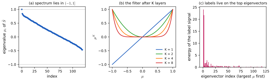
Spectrum of \(\hat{\bm S}\). \(\hat{\bm S}\) is the normalised adjacency matrix of the graph with self loops, and the same computation as above gives \(\bm I-\hat{\bm S}\in[0,2]\), i.e. eigenvalues of \(\hat{\bm S}\) in \([-1,1]\). Moreover \(\hat{\bm S}\tilde{\bm D}^{1/2}\mathbf 1=\tilde{\bm D}^{-1/2}\tilde{\bm A}\mathbf 1=\tilde{\bm D}^{1/2}\mathbf 1\), so \(1\) is an eigenvalue with eigenvector \(\bm v_1\propto\tilde{\bm D}^{1/2}\mathbf 1\); and the eigenvalue \(-1\) is excluded: \(\hat{\bm S}\bm v=-\bm v\) requires \(\sum_{ij}\tilde A_{ij}(x_i+x_j)^2=0\) for \(\bm x=\tilde{\bm D}^{-1/2}\bm v\), but \(\tilde A_{ii}=1\) forces \(x_i=0\) for every \(i\), so \(\bm v=\bm 0\). Hence the spectrum lies in \((-1,1]\), and \(1-\mu\in[0,2)\) for every eigenvalue \(\mu\) of \(\hat{\bm S}\) (the version without self loops can have eigenvalue \(-1\) on bipartite graphs, where signals alternate sign forever). Numerical confirmation. On a 90-node planted-partition graph \(\hat{\bm S}\) has all eigenvalues in \((-1,1]\), the top eigenvalue is 1 with eigenvector \(\tilde{\bm D}^{1/2}\mathbf 1\) to \(10^{-10}\); the normalised Laplacian of the karate club has largest eigenvalue 1.71 (\(\le2\)); and \(\theta(\bm I+\bm D^{-1/2}\bm A\bm D^{-1/2})\bm x\) equals the spectral filter \(\theta(2-\lambda)\) to \(10^{-9}\) (Figure 23.S5a, b).
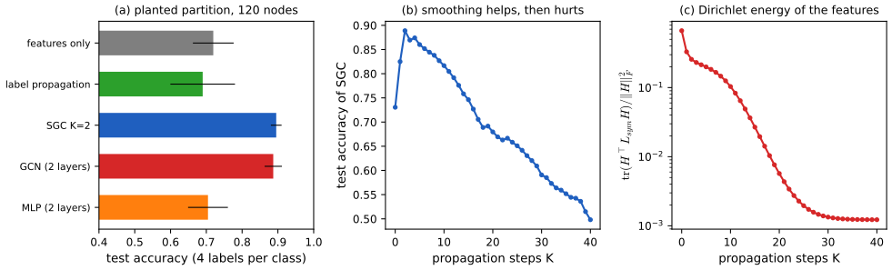
Over-smoothing. Let the graph be connected. The eigenvalues of \(\hat{\bm S}\) are \(1=\mu_1>\mu_2\ge\dots\ge\mu_N>-1\), so with the orthogonal projector \(\bm P_1=\bm v_1\bm v_1^\T/\|\bm v_1\|^2\), \[ \hat{\bm S}^K\bm X=\sum_k\mu_k^K\bm v_k\bm v_k^\T\bm X\ \longrightarrow\ \bm P_1\bm X\quad(K\to\infty),\qquad\|\hat{\bm S}^K\bm X-\bm P_1\bm X\|_F\le\max(|\mu_2|,|\mu_N|)^K\|\bm X\|_F.\] In the limit all rows are proportional to \(\sqrt{d_i+1}\): every node has the same feature direction, with a scale fixed by its degree, and the information distinguishing nodes is gone; the rate is the spectral gap \(1-\max(|\mu_2|,|\mu_N|)\). A nonlinearity and weights between the layers change the rate but not the phenomenon (companion course, DL 13.3.4). The Dirichlet energy \(\operatorname{tr}(\bm H^\T\bm L_{\rm sym}\bm H)/\|\bm H\|_F^2=\sum_k\lambda_k\|\bm v_k^\T\bm H\|^2/\sum_k\|\bm v_k^\T\bm H\|^2\) is a weighted average of the frequencies of \(\bm H\) that, for \(\bm H=\hat{\bm S}^K\bm X\), is non-increasing in \(K\): the weights \(\mu_k^{2K}\) shift towards the top (low-frequency) eigenvectors. (Here \(\bm L_{\rm sym}\) is that of the graph without self loops, so the energy approaches a small positive value, not zero, as in Figure 23.S4c.) Numerical confirmation. \(\hat{\bm S}^{200}\bm X\) equals \(\bm P_1\bm X\) to \(10^{-15}\) on the 90-node graph, and the Dirichlet energy is non-increasing over \(K=0,\dots,29\).
Why smoothing helps first. If node features are class means plus independent noise and the graph is homophilous, averaging over a neighbourhood of about \(\bar d\) nodes of the same class divides the noise variance by about \(\bar d\) while keeping the class mean. A large share of the label signal (57 percent in Figure 23.S5c) lives on the leading eigenvectors of \(\hat{\bm S}\), which are exactly those that survive the filter \(\mu^K\) (Figure 23.S5b). After a few steps the surviving components are those between communities (still useful) and then only the global projector (useless). \(\square\)
See also: graph convolutional networks and over-smoothing in Foundations of Deep Learning.
23.4.3 Spatial Graph Convolutions
p. 763 Spectrum-based filters depend on the spectrum of one graph and spectrum-free ones need the whole graph. Spatial methods define convolutions on fixed-size neighbourhoods in the vertex domain, by neighbourhood sampling or by attention, to obtain patches of fixed size from irregular graphs and to allow inductive learning.
23.4.3.1 Sampling-based spatial methods
pp. 763–764 GraphSAGE (Hamilton, Ying and Leskovec) samples \(q\) neighbours of each node instead of using all of them, so the cost per node is fixed and the model applies to graphs not seen in training. A layer is \[ \bm H^{\ell+1}_{:,i}=\sigma\Big(\bm\Theta_1^\ell\bm H^\ell_{:,i}+\bm\Theta_2^\ell\,\mathrm{AGG}\big(\{\bm H^\ell_{:,j}:v_j\in\mathrm{Sample}(\mathrm{nbr}(v_i),q)\}\big)\Big),\tag{23.27} \] with a permutation-invariant AGG (mean, max-pool). Figure 23.5 of the book illustrates the sampling and is not reproduced. Gap 23.12 quantifies the noise that sampling introduces.
Filling the gap 23.12: the mean of sampled neighbours is unbiased, with a finite-population variance p. 764, (23.27)
Derivation
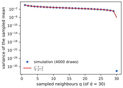
Let node \(i\) have \(d\) neighbours with (scalar, for one feature coordinate) values \(h_1,\dots,h_d\), mean \(\bar h\) and population variance \(\sigma^2=\frac1d\sum_k(h_k-\bar h)^2\). Draw \(q\le d\) of them uniformly without replacement, as a simple random sample \(S\), and let \(\hat h=\frac1q\sum_{k\in S}h_k\). Write \(\hat h=\frac1q\sum_{k=1}^dI_kh_k\) with \(I_k=\mathbb 1(k\in S)\), \(\E I_k=\frac qd\), \(\var I_k=\frac qd(1-\frac qd)\), and for \(k\ne l\), \(\cov(I_k,I_l)=\frac{q(q-1)}{d(d-1)}-\frac{q^2}{d^2}=-\frac{q(d-q)}{d^2(d-1)}\). Then \(\E\hat h=\frac1q\cdot\frac qd\sum_kh_k=\bar h\) (unbiased), and with \(h_k-\bar h=:e_k\), \(\sum_ke_k=0\), \[ \var\hat h=\frac1{q^2}\Big[\sum_ke_k^2\var I_k+\sum_{k\ne l}e_ke_l\cov(I_k,I_l)\Big]=\frac1{q^2}\Big[\frac{q(d-q)}{d^2}\sum_ke_k^2+\frac{q(d-q)}{d^2(d-1)}\sum_ke_k^2\Big]\] using \(\sum_{k\ne l}e_ke_l=(\sum_ke_k)^2-\sum_ke_k^2=-\sum_ke_k^2\), which turns the covariance term into \(+\frac{q(d-q)}{d^2(d-1)}\sum_ke_k^2\). The bracket is therefore \(\frac{q(d-q)}{d^2}\sum_ke_k^2\big(1+\frac1{d-1}\big)=\frac{q(d-q)}{d(d-1)}\sum_ke_k^2\), and with \(\sum_ke_k^2=d\sigma^2\), \[ \var\hat h=\frac1{q^2}\cdot\frac{q(d-q)}{d(d-1)}\,d\sigma^2=\frac{\sigma^2}{q}\cdot\frac{d-q}{d-1}.\] So the variance is the with-replacement value \(\sigma^2/q\) times the finite-population correction \(\frac{d-q}{d-1}\), which is \(1\) for \(q=1\) and \(0\) when all neighbours are used (\(q=d\)). Averaging in the aggregator is therefore an unbiased estimate of the full neighbourhood mean, and doubling \(q\) roughly halves the variance. Numerical confirmation. Enumerating all \(\binom73=35\) subsets of 7 values gives mean \(\bar h\) and variance \(\frac{\sigma^2}{3}\frac{4}{6}\) exactly; simulation with \(d=12\) and \(q=1,4,9\) agrees within sampling error, and Figure 23.S6 shows the formula against 4000 draws for \(d=30\). \(\square\)
23.4.3.2 Attention-based spatial methods
p. 764 Graph attention networks (GAT, Veličković et al.) learn, for each node, how much to weight each neighbour: scores computed from the two nodes' (transformed) features are normalised by a softmax over the neighbourhood. Unlike GraphSAGE, GAT attends to the whole neighbourhood and gives each neighbour a learned weight; unlike a GCN the weights depend on the features.
Filling the gap 23.13: the attention layer, and its relation to mean aggregation p. 764
Derivation
One head: with a weight matrix \(\bm\Theta\) and vectors \(\bm a_1,\bm a_2\), the (pre-)attention score is \(e_{ij}=\mathrm{LeakyReLU}(\bm a_1^\T\bm\Theta\bm h_i+\bm a_2^\T\bm\Theta\bm h_j)\) for \(j\in\mathcal N(i)\cup\{i\}\), the weights \(\alpha_{ij}=\frac{\exp e_{ij}}{\sum_{k\in\mathcal N(i)\cup\{i\}}\exp e_{ik}}\), and the output \(\bm h_i'=\sum_j\alpha_{ij}\bm\Theta\bm h_j\) (followed by a nonlinearity). Facts: (i) \(\alpha_{ij}\ge0\), \(\sum_j\alpha_{ij}=1\): the output is a convex combination of the neighbours' transformed features, a data-dependent weighted mean. (ii) If \(\bm a_1=\bm a_2=\bm 0\), all scores vanish and \(\alpha_{ij}=1/(|\mathcal N(i)|+1)\): the layer is the neighbourhood mean (a GCN with random-walk normalisation), so attention strictly generalises mean aggregation. (iii) Permutation equivariance as in gap 23.10, because \(\alpha_{ij}\) depends only on the features of \(i\) and \(j\) and the softmax normalises over a set. (iv) The scores are a sum of a node-\(i\) term and a node-\(j\) term before the LeakyReLU, so a layer's scores cost \(O(M)\) and are not a query-key dot product as in transformer attention. Because LeakyReLU is monotone, the ranking of the neighbours \(j\) of \(i\) by \(e_{ij}\) is the same for every \(i\) (it is the ranking of \(\bm a_2^\T\bm\Theta\bm h_j\)): this "static attention" limitation was pointed out by Brody et al. (2022); only the sharpness of the weights depends on the receiving node. Numerical confirmation. On the karate club the rows of \(\bm\alpha\) sum to 1, a random relabelling of the nodes permutes the output accordingly (\(10^{-10}\)), and zero attention parameters give the uniform neighbourhood mean. \(\square\)
23.4.3.3 Geometric spatial methods
p. 765 MoNet (Monti et al.) is designed for nodes with geometric (pseudo-)coordinates, such as meshes or point clouds. With pseudo-coordinates \(\bm U^s\) it learns \(K\) parametric patches \(g_k(\bm U^s)\) (each an \(N\times N\) matrix) and uses \[ \bm H^{\ell+1}=\sigma\Big(\sum_{k=1}^K\big(\bm W\odot g_k(\bm U^s)\big)\bm H^\ell\bm\Theta^\ell_k\Big),\qquad g_k(\bm U^s)=\exp\!\Big(-\tfrac12(\bm U^s-\bm\mu_k)^\T\bm\Sigma_k^{-1}(\bm U^s-\bm\mu_k)\Big),\tag{23.28, 23.29} \] with learned \(\bm\mu_k\) and diagonal \(\bm\Sigma_k\). It generalises the geodesic and anisotropic CNNs, whose patches are fixed on a specific coordinate system. (Each \(g_k\) is a Gaussian weight on a pair's pseudo-coordinate: a soft assignment of the neighbour to the \(k\)-th "direction", exactly as the position in a pixel patch selects the filter tap in an ordinary convolution.)
23.4.4 Non-Euclidean Graph Convolutions
p. 765 Shallow hyperbolic embeddings (Section 23.3.3) do not generalise to new graphs, while GNNs use node features. Hyperbolic graph convolutional networks (HGCN, Chami et al.; HGNN, Liu et al.) combine the two: at every layer node embeddings are mapped to the Euclidean tangent space at the origin (a first-order approximation of the manifold, \(\log_{\bm 0}\)), a Euclidean graph convolution is applied there, and the result is mapped back to the hyperbolic space (\(\exp_{\bm0}\)). On the Poincaré ball with the metric of gap 23.14 these maps are \(\exp_{\bm 0}(\bm v)=\tanh(\|\bm v\|)\,\bm v/\|\bm v\|\) and \(\log_{\bm0}(\bm x)=\artanh(\|\bm x\|)\,\bm x/\|\bm x\|\): the metric at the origin is \(4\|\d\bm x\|^2\), so a tangent vector \(\bm v\) has length \(2\|\bm v\|\) and the geodesic of that length ends at radius \(\tanh(\|\bm v\|)\), consistent with \(d(\bm0,\bm x)=2\artanh\|\bm x\|\). These maps give significant improvements on hierarchical graphs (Figure 23.6 of the book, a drawing of GCN against HGCN embeddings of a tree; our Figure 23.6 above compares the two geometries with shallow embeddings and the demo shows the effect of edge length).
23.5 Deep graph embeddings
p. 765 Here a GNN is the encoder and the loss is unsupervised or semi-supervised. Figure 23.7 of the book (the unsupervised GNN pipeline) is a diagram and is not reproduced.
23.5.1 Unsupervised embeddings
23.5.1.1 Structural deep network embedding
p. 766 SDNE (Wang et al.) feeds a row of the adjacency matrix to an auto-encoder, \(\bm Z=\ENC(\bm W;\bm\theta_E)\) (node features are ignored), and decodes \(\widehat{\bm W}=\DEC(\bm Z;\bm\Theta_D)\) without an outer product. Its loss combines a second-order proximity term (nodes with similar neighbourhoods get similar embeddings, through reconstruction of the row) and a first-order term, the Laplacian-eigenmaps penalty of Section 23.3.2: \[ \big\|(s(\bm W)-\widehat{\bm W})\odot\mathbb I(s(\bm W)>0)\big\|_F^2+\alpha_{\rm SDNE}\sum_{ij}s(\bm W)_{ij}\|\bm z_i-\bm z_j\|_2^2.\tag{23.30} \] The first term is the matrix-factorisation objective with a mask over the observed edges, as in graph factorisation (gap 23.3), but with a nonlinear decoder.
23.5.1.2 (Variational) graph auto-encoders
p. 767 The graph auto-encoder (GAE, Kipf and Welling) encodes with a graph convolutional network, \(\bm Z=\mathrm{GCN}(\bm W,\bm X;\bm\Theta_E)\), and decodes by an inner product, \(\widehat{\bm W}=\bm Z\bm Z^\T\), with the sigmoid cross-entropy reconstruction loss \[ \mathcal L_{G,{\rm RECON}}(\bm W,\widehat{\bm W};\bm\Theta)=-\Big(\sum_{ij}(1-W_{ij})\log\big(1-\sigma(\widehat W_{ij})\big)+W_{ij}\log\sigma(\widehat W_{ij})\Big).\tag{23.31} \] The sum over all \(N^2\) pairs is expensive; GAE samples negative pairs. The variational graph auto-encoder (VGAE) treats \(\bm Z\) as a latent variable with prior \(p(\bm Z)=\N(\bm Z\given\bm0,\bm I)\) and a GCN as inference network \(q_\phi(\bm Z\given\bm W,\bm X)\), and minimises the negative ELBO \[ \mathrm{NELBO}(\bm W,\bm X;\bm\Theta)=-\E_{q_\phi(\bm Z\given\bm W,\bm X)}[\log p(\bm W\given\bm Z)]+\KL\big(q_\phi(\bm Z\given\bm W,\bm X)\,\|\,p(\bm Z)\big)\tag{23.32} \] \[ =\mathcal L_{G,{\rm RECON}}(\bm W,\widehat{\bm W};\bm\Theta)+\KL\big(q_\phi(\bm Z\given\bm W,\bm X)\,\|\,p(\bm Z)\big).\tag{23.33} \]
Filling the gap 23.16: the GAE loss as a Bernoulli likelihood, and the VGAE bound p. 767, (23.31)–(23.33)
Derivation
(23.31) is a Bernoulli negative log-likelihood. Model each pair independently, \(p(W_{ij}\given\bm Z)=\mathrm{Ber}\big(W_{ij}\given\sigma(\bm z_i^\T\bm z_j)\big)\). Then \(-\log p(\bm W\given\bm Z)=-\sum_{ij}\big[W_{ij}\log\sigma(\widehat W_{ij})+(1-W_{ij})\log(1-\sigma(\widehat W_{ij}))\big]\), which is (23.31). Using \(\log\sigma(a)=-\operatorname{softplus}(-a)\) and \(\log(1-\sigma(a))=-\operatorname{softplus}(a)\), the loss equals \(\sum_{ij}\big[\operatorname{softplus}(\widehat W_{ij})-W_{ij}\widehat W_{ij}\big]\). Because most pairs are non-edges, implementations re-weight the positive terms (by \((N^2-M)/M\)) or sample negatives, which changes the objective to a weighted likelihood but not the model. Numerical confirmation. The two forms agree to machine precision on a random example.
The ELBO. For any \(q_\phi(\bm Z\given\cdot)\), Jensen's inequality gives \(\log p(\bm W)=\log\int p(\bm W\given\bm Z)p(\bm Z)\d\bm Z=\log\E_q\big[\frac{p(\bm W\given\bm Z)p(\bm Z)}{q(\bm Z)}\big]\ge\E_q[\log p(\bm W\given\bm Z)]-\KL(q\|p)\), and the gap is \(\KL(q\|p(\bm Z\given\bm W))\ge0\) (the same derivation as the VAE bound of Section 20.3.5). Minus the right side is (23.32). With a diagonal Gaussian posterior \(q=\prod_{i,l}\N(\mu_{il},\sigma_{il}^2)\) and prior \(\N(0,1)\), the KL is available in closed form, \[ \KL=\frac12\sum_{i,l}\big(\sigma_{il}^2+\mu_{il}^2-1-\log\sigma_{il}^2\big)\] (per coordinate, \(\E_q\log q-\E_q\log p=-\frac12\log\sigma^2-\frac12+\frac12(\sigma^2+\mu^2)\)), while the reconstruction expectation is estimated by one reparametrised sample \(\bm Z=\bm\mu+\bm\sigma\odot\bm\varepsilon\), \(\bm\varepsilon\sim\N(\bm 0,\bm I)\). Numerical confirmation. The closed-form KL for 500 random \((\mu,\log\sigma^2)\) agrees with a Monte Carlo estimate from 40,000 samples (270.28 against 270.36). \(\square\)
23.5.1.3 Iterative generative modelling of graphs (Graphite)
p. 767 Graphite (Grover et al.) enriches the decoder of GAE/VGAE by alternating a pairwise decoding with a graph convolution: \[ \widehat{\bm W}^{(k)}=\frac{\bm Z^{(k)}\bm Z^{(k)\T}}{\|\bm Z^{(k)}\|_2^2}+\frac{\mathbf 1\mathbf 1^\T}{N},\qquad\bm Z^{(k+1)}=\mathrm{GCN}\big(\widehat{\bm W}^{(k)},\bm Z^{(k)}\big),\] with \(\bm Z^{(0)}\) the encoder output; the normalised inner product plus the constant matrix is a dense, row-comparable proximity matrix used as the graph for the next convolution. Like GAE it can be deterministic or variational.
23.5.1.4 Methods based on contrastive losses
pp. 767–768 Deep graph infomax (DGI, Veličković et al.) makes up fake graphs \((\bm W^-,\bm X^-)\) (same adjacency, features permuted by rows), encodes both real and fake graphs with a shared GCN, summarises each by a readout (e.g. the row-wise mean), and trains a discriminator \(D\) to output close to 1 for (node, summary) pairs of the real graph and close to 0 for the fake one: \[ \min_{\bm\Theta}\ -\E_{\bm X,\bm W}\sum_{i=1}^N\log D\big(\bm z_i,R(\bm Z)\big)-\E_{\bm X^-,\bm W^-}\sum_{j=1}^{N^-}\log\Big(1-D\big(\bm z_j^-,R(\bm Z^-)\big)\Big).\tag{23.34} \] This is claimed to maximise a lower bound on the mutual information between node and graph representations; a variant (graphical mutual information, Peng et al.) uses node and neighbourhood instead. Gap 23.17 states and proves what the bound is.
Filling the gap 23.17: the discriminator loss and a mutual-information bound p. 768, (23.34)
Derivation
Setting. Let \(p\) be the distribution of the positive pairs \((\bm z,\bm s)\) (node embedding, summary) and \(q\) that of the negative pairs. Per pair, the loss in (23.34) is \(\ell(D)=\E_p[-\log D]+\E_q[-\log(1-D)]\) (the book sums over nodes; the per-pair normalisation does not change the minimiser).
Optimal discriminator. Pointwise, \(-p(x)\log D(x)-q(x)\log(1-D(x))\) is minimised at \(D^\ast(x)=\frac{p(x)}{p(x)+q(x)}\) (set the derivative \(-\frac pD+\frac q{1-D}\) to zero; convexity in \(D\)). With \(m=\frac{p+q}2\), \(D^\ast=\frac p{2m}\), \(1-D^\ast=\frac q{2m}\), and \[ \ell(D^\ast)=-\E_p\log\frac p{2m}-\E_q\log\frac q{2m}=2\log2-\KL(p\|m)-\KL(q\|m)=2\log2-2\,\JSD(p,q),\] where \(\JSD(p,q)=\frac12\KL(p\|m)+\frac12\KL(q\|m)\) is the Jensen–Shannon divergence. For any other discriminator \(\ell(D)\ge\ell(D^\ast)\), so \(2\log2-\ell(D)\le2\,\JSD(p,q)\) always.
Relation to mutual information. Suppose the negative pairs follow the product of the marginals of the positive ones, \(q=p_{\bm z}\otimes p_{\bm s}\); then \(\KL(p\|q)=I(\bm z;\bm s)\), the mutual information. Expanding the mixture, \(\KL(p\|m)\) and \(\KL(q\|m)\) satisfy \(\tfrac12\KL(p\|q)-\JSD(p,q)=\KL(m\|q)\ge0\) (compute \(\tfrac12\KL(p\|q)-\tfrac12\KL(p\|m)-\tfrac12\KL(q\|m)=\tfrac12\E_p\log\frac mq+\tfrac12\E_q\log\frac mq=\E_m\log\frac mq\)). Hence \[ 2\log2-\ell(D)\ \le\ 2\,\JSD(p,q)\ =\ \KL(p\|q)-2\KL(m\|q)\ \le\ I(\bm z;\bm s),\] so minimising (23.34) maximises a lower bound on the mutual information, as claimed. Caveats: the bound is on the Jensen–Shannon quantity, which is a weaker proxy than the KL-based mutual information (it is bounded by \(\log2\) while \(I\) is not), and DGI's negatives (permuted features on the same graph) only approximate the product of marginals, so the statement is heuristic for the method itself. Numerical confirmation. For random discrete \(p,q\) the loss at \(D^\ast\) equals \(2\log2-2\JSD\) to machine precision and \(\JSD=\frac12\KL(p\|q)-\KL(m\|q)\); for a random \(4\times5\) joint distribution \(2\JSD(p,p_{\bm z}p_{\bm s})=0.121\le I=0.212\). \(\square\)
23.5.2 Semi-supervised embeddings
p. 768 The simple special case here uses a nonlinear encoder of the node features and ignores the graph structure in the encoder, \(\bm Z=\ENC(\bm X;\bm\Theta_E)\), using the graph only in the loss.
23.5.2.1 SemiEmb
p. 768 SemiEmb (Weston et al.) encodes with an MLP and decodes with a distance, \(\widehat W_{ij}=\|\bm z_i-\bm z_j\|\) (\(L_2\) or \(L_1\)); it regularises intermediate or auxiliary layers with the label-propagation loss (23.19) and predicts labels from intermediate embeddings with a feed-forward network and a hinge loss. It is the neural analogue of Laplacian regularisation in label propagation (gap 23.8): the penalty \(\sum_{ij}W_{ij}\|\bm z_i-\bm z_j\|^2\) is the Dirichlet energy (gap 23.1) of the embedding.
23.5.2.2 Planetoid
pp. 768–769 Skip-gram methods learn embeddings in two steps (generate walks, then train), which need not suit a classification task. Planetoid (Yang et al.) maps nodes to \(\bm Z=[\bm Z^c\,\|\,\bm Z^F]=\ENC(\bm X;\bm\Theta_E)\), where \(\bm Z^c\) captures structure (a look-up table in the transductive version, a function of the features in the inductive version) and \(\bm Z^F\) captures features. Its objective has a graph term that predicts context, \[ \mathcal L_{G,{\rm RECON}}(\bm W,\widehat{\bm W};\bm\Theta)=-\E_{(i,j,\gamma)}\log\sigma\big(\gamma\widehat W_{ij}\big),\qquad\widehat W_{ij}=\bm z_i^\T\bm z_j,\tag{23.35} \] with \(\gamma=+1\) for a positive pair \((v_i,v_j)\in\mathcal E\) and \(\gamma=-1\) for a negative pair (the distribution is defined by a sampling process), and a supervised term, the cross entropy of labels on the labelled nodes, \[ \mathcal L^{\mathcal N}_{\rm SUP}(\bm y^{\mathcal N},\hat{\bm y}^{\mathcal N};\bm\Theta)=-\frac1{|V_L|}\sum_{i:v_i\in V_L}\sum_{k=1}^{C}y^{\mathcal N}_{ik}\log\hat y^{\mathcal N}_{ik}.\tag{23.36} \] Since \(\sigma(-a)=1-\sigma(a)\), (23.35) is exactly the positive and negative terms of skip-gram with negative sampling (gap 23.7): \(-\log\sigma(\widehat W_{ij})\) for a positive pair and \(-\log(1-\sigma(\widehat W_{ij}))\) for a negative one.
23.6 Applications
p. 769 The book lists applications of unsupervised and supervised graph embeddings.
23.6.1 Unsupervised applications
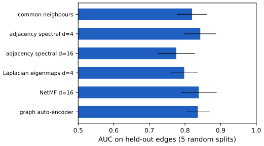
pp. 769–771 Graph reconstruction (23.6.1.1) asks for embeddings from which the graph can be recovered, measured by reconstruction error: it is dimensionality reduction for graphs (Sections 23.3.1 and 23.5.1). Link prediction (23.6.1.2) predicts missing or future edges (friendships, user-item links, suspicious transactions as in Figure 23.8, missing relations in a knowledge graph). The usual protocol hides a fraction of the edges (and samples as many non-edges), trains on the rest and ranks the held-out pairs; it differs from reconstruction, where nothing is held out. Edge labels are not used in training, so the book files link prediction under the unsupervised applications. Figure 23.S7 compares scores on a planted-partition graph. Clustering (23.6.1.3) applies k-means or another algorithm to the embeddings, or learns clusters jointly with the embedding. Visualisation (23.6.1.4) maps embeddings to two dimensions with t-SNE or PCA, colouring nodes by attributes (Figure 23.S1 does this directly with two-dimensional embeddings).
23.6.2 Supervised applications
pp. 771–772 Node classification (23.6.2.1; sometimes called statistical relational learning) predicts node labels, typically semi-supervised and transductive (one partially labelled graph); node features can add a great deal when informative, which is why GCN and GraphSAGE beat random-walk methods that ignore features (Figure 23.S4a: on the planted-partition task, a GCN reaches 0.89 where features alone give 0.72 and the graph alone 0.69). Graph classification (23.6.2.2) predicts a label for a whole graph, as for the toxicity or odour of a molecule (Figure 23.9, molecule pictures, not reproduced), is inductive, and needs a pooling operation that turns node embeddings into a graph embedding; permutation invariance (gap 23.10) requires a symmetric pooling such as the sum or mean over nodes.
Exercises
The April 2025 draft of the book has no end-of-chapter exercises for Chapter 23. These three supplementary exercises (numbered S1 to S3) practise the main computations; each has a complete worked solution (hidden).
Exercise 23.S1 (receptive fields and sampling). In the karate-club graph, member 34 has the largest degree, 17. (a) How many nodes lie within one hop and within two hops of it (itself included)? (b) A two-layer GraphSAGE network samples \(q=3\) neighbours at each layer. What is the largest number of distinct nodes whose features can reach node 34's output, and is sampling worth it on this graph?
Solution
(a) By gap 23.10, \((\bm A+\bm I)^\ell\) has a positive \((i,j)\) entry iff the hop distance is at most \(\ell\). Counting the positive entries in row 34 of \((\bm A+\bm I)\) and \((\bm A+\bm I)^2\) gives 18 nodes within one hop (the node and its 17 neighbours) and 24 within two hops (and all 33 nodes in the other 33 are within three hops, a diameter-5 graph).
(b) Sampling \(q=3\) neighbours of the node and \(q=3\) neighbours of each of those gives at most \(1+3+3\cdot3=13\) distinct nodes, against 24 for full aggregation: the cost is bounded independently of the degrees. On this small graph the saving is modest (24 against 13) and it costs variance \(\frac{\sigma^2}{3}\frac{17-3}{16}\) per aggregation (gap 23.12); the benefit appears on graphs where the two-hop ball is far larger than \(q^2\), such as social networks with hub nodes. (With \(q=5\) the bound \(1+5+25=31\) would exceed 24: sampling cannot reach more than the ball and is useless there.) \(\square\)
Exercise 23.S2 (a hyperbolic distance). Two points of the Poincaré disk are at the same Euclidean radius \(r\) on opposite sides of the origin, \(\bm x=(r,0)\), \(\bm y=(-r,0)\). Find \(d(\bm x,\bm y)\) from (23.11) and compare it with the Euclidean distance. For \(r=0.9\) give the numbers.
Solution
\(\|\bm x-\bm y\|^2=4r^2\), so \(1+\frac{2\cdot4r^2}{(1-r^2)^2}=\frac{(1-r^2)^2+8r^2}{(1-r^2)^2}=\frac{1+6r^2+r^4}{(1-r^2)^2}\), and \(d=\arcosh\frac{1+6r^2+r^4}{(1-r^2)^2}\). Using \(\cosh(2u)=2\cosh^2u-1\) with \(\cosh u=\frac{1+r^2}{1-r^2}\) (the half-distance, \(u=2\artanh r\)) gives \(2\frac{(1+r^2)^2}{(1-r^2)^2}-1=\frac{1+6r^2+r^4}{(1-r^2)^2}\), so \(d=2u=4\artanh r\): the geodesic is the diameter through the origin, of length twice \(d(\bm0,\bm x)\). For \(r=0.9\): \(4\artanh0.9=5.889\) (and \(\arcosh(1+2\cdot3.24/0.0361)=\arcosh(180.5)=5.889\)), against a Euclidean distance of 1.8 and a Euclidean diameter of at most 2: points that look only twice as far from each other as from the origin are 5.9 units apart, and as \(r\to1\), \(d\sim2\ln\frac{2}{1-r}\to\infty\). \(\square\)
Exercise 23.S3 (label propagation on a path). A path graph has nodes \(1,\dots,n\) joined in a line with unit weights, node 1 labelled 0 and node \(n\) labelled 1. Find the harmonic solution, and show that the iteration \(f_i\leftarrow\frac12(f_{i-1}+f_{i+1})\) converges to it.
Solution
For an interior node, harmonicity (gap 23.8) says \(f_i=\frac12(f_{i-1}+f_{i+1})\), i.e. \(f_{i+1}-f_i=f_i-f_{i-1}\): the increments are constant, so \(f\) is linear, and the boundary values give \(f_i=\frac{i-1}{n-1}\). It is unique (gap 23.8: \(\bm L_{UU}\) is positive definite since both components have a labelled node). The iteration is the map \(\bm f_U\leftarrow\bm P_{UU}\bm f_U+\bm P_{UL}\bm f_L\) with \(\bm P_{UU}\) the tridiagonal matrix with entries \(\frac12\) beside the diagonal, whose eigenvalues are \(\cos\frac{k\pi}{n-1}\), \(k=1,\dots,n-2\) (the eigenvectors are sines), so the spectral radius is \(\cos\frac\pi{n-1}<1\) and the error shrinks by about \(1-\frac{\pi^2}{2(n-1)^2}\) per sweep: for long paths the convergence is slow, in proportion to \(n^2\). Check: for \(n=9\) the code returns \(i/8\) to \(10^{-12}\). \(\square\)
Demonstrations
| Page | What it shows | In the notes |
|---|---|---|
| Shallow embeddings of the karate club | Laplacian eigenmaps, MDS on hop distances, adjacency spectral and NetMF (the closed-form target of DeepWalk) in two dimensions, with window length, number of negatives and window distribution. Presets: 1 Laplacian eigenmaps; 2 MDS; 3 adjacency spectral; 4 NetMF window 5; 5 many negatives; 6 window 1. | 23.3.2, 23.3.4, 23.3.5, gap 23.7 |
| Label propagation | Two half-moons joined by a nearest-neighbour graph: the clamped iteration, its harmonic limit and label spreading, with the number of labels, graph density, sweeps and spreading parameter. Presets: 1 ten sweeps; 2 after 1000 sweeps; 3 harmonic, three labels; 4 eight labels; 5 spreading; 6 sparse graph. | 23.3.6, gap 23.8 |
| Graph convolution as feature smoothing | Simplified GCN on a three-community graph with overlapping features: test accuracy and Dirichlet energy against the number of propagation steps, decision regions in the smoothed feature plane. Presets: 1 no propagation; 2 two layers; 3 ten layers; 4 over-smoothing; 5 one label per class. | 23.4.2, gap 23.11 |
| Trees in the Poincaré disk | A complete tree embedded with equal edge lengths in the Poincaré disk (geodesics drawn) and in the Euclidean plane, with distortion by tree distance. Presets: 1 binary, depth 5; 2 long edges; 3 short edges; 4 ternary tree; 5 depth 7. | 23.3.3, gap 23.14 |
The Python code that produces every figure of this page is code/ch23_graph_embeddings.py (see the code index). Companion demos: spectral clustering and PageRank (ESL), PCA (Bishop).
Notes on the book
Points where the book is imprecise or wrong
- (23.17), the window distribution. \(P(Q=q)=\frac{T_{\max}-1+q}{T_{\max}}\) is not a probability distribution: for \(q=T_{\max}\) it equals \(2-\frac1{T_{\max}}>1\), the values increase with \(q\), and they sum to \(\frac{3T_{\max}-1}2\) (7 for \(T_{\max}=5\)). The uniform window gives \(1/T_{\max}\) and the word2vec dynamic window \(\frac{2(T_{\max}+1-q)}{T_{\max}(T_{\max}+1)}\), decreasing in \(q\) (gap 23.5, Figure 23.S2a).
- (23.16), GraRep target. The \(k\)-step transition matrix is \((\bm D^{-1}\bm W)^k\), which is row-stochastic; \(\bm D^{-k}\bm W^k\) as printed is a different matrix (differing by up to 0.94 in one entry on the karate club for \(k=2\)) and is not row-stochastic (gap 23.4).
- (23.19), the labels. The graph term is printed as \(\sum_{ij}W_{ij}\|\bm y_i^{\mathcal N}-\hat{\bm y}_j^{\mathcal N}\|^2\), mixing the true label of \(i\) with the predicted label of \(j\); the smoothness term compares predictions, \(\|\hat{\bm y}_i-\hat{\bm y}_j\|^2\), as in (23.20) (gap 23.8).
- (23.12), sign. As printed it is a sum of log-probabilities to be maximised; the loss to minimise is its negative (gap 23.15).
- (23.9), factor \(\frac12\). \(\operatorname{tr}(\bm Z^\T\bm L\bm Z)=\frac12\sum_{ij}W_{ij}\|\bm z_i-\bm z_j\|^2\), so (23.9)–(23.10) represent the objective only up to the factor \(\frac12\); this does not change the minimiser (gap 23.1).
- Section 23.4.1, "Almeda-Pineda". The algorithm of Almeida (1987) and Pineda (1988) (gap 23.9).
- Section 23.5.1.4, "lower bound on the mutual information". What the DGI loss lower-bounds is the Jensen–Shannon quantity \(2\JSD(p,q)\), which is itself at most the mutual information when the negatives follow the product of marginals; permuted-feature negatives only approximate this (gap 23.17).
- Section 23.3.3, "(23.12) denominator". The sum runs over the unrelated nodes only and, as the text says, is approximated by negative sampling; the positive node should be included in the softmax denominator, as in the original paper (the printed form has the positive term outside the normaliser), see gap 23.15.
References
- Murphy, K. P. (2022). Probabilistic Machine Learning: An Introduction. MIT Press, Cambridge, MA. Chapter 23, pp. 753–772. probml.github.io/pml-book/book1.html.
- Ahmed, A., Shervashidze, N., Narayanamurthy, S., Josifovski, V. and Smola, A. J. (2013). Distributed large-scale natural graph factorization. Proceedings of the 22nd International Conference on World Wide Web.
- Almeida, L. B. (1987). A learning rule for asynchronous perceptrons with feedback in a combinatorial environment. Proceedings of the IEEE First International Conference on Neural Networks.
- Battaglia, P. W. et al. (2018). Relational inductive biases, deep learning, and graph networks. arXiv:1806.01261.
- Belkin, M. and Niyogi, P. (2003). Laplacian eigenmaps for dimensionality reduction and data representation. Neural Computation, 15(6), 1373–1396.
- Brody, S., Alon, U. and Yahav, E. (2022). How attentive are graph attention networks? International Conference on Learning Representations.
- Cao, S., Lu, W. and Xu, Q. (2015). GraRep: learning graph representations with global structural information. Proceedings of the 24th ACM International Conference on Information and Knowledge Management.
- Chami, I., Abu-El-Haija, S., Perozzi, B., Ré, C. and Murphy, K. (2021). Machine learning on graphs: a model and comprehensive taxonomy. arXiv:2005.03675.
- Chami, I., Ying, R., Ré, C. and Leskovec, J. (2019). Hyperbolic graph convolutional neural networks. Advances in Neural Information Processing Systems, 32.
- Gilmer, J., Schoenholz, S. S., Riley, P. F., Vinyals, O. and Dahl, G. E. (2017). Neural message passing for quantum chemistry. International Conference on Machine Learning.
- Grover, A., Zweig, A. and Ermon, S. (2019). Graphite: iterative generative modeling of graphs. International Conference on Machine Learning.
- Hamilton, W. L., Ying, R. and Leskovec, J. (2017). Inductive representation learning on large graphs. Advances in Neural Information Processing Systems, 30.
- Kipf, T. N. and Welling, M. (2016). Semi-supervised classification with graph convolutional networks. arXiv:1609.02907. And (2016), Variational graph auto-encoders, arXiv:1611.07308.
- Levy, O. and Goldberg, Y. (2014). Neural word embedding as implicit matrix factorization. Advances in Neural Information Processing Systems, 27.
- Monti, F., Boscaini, D., Masci, J., Rodolà, E., Svoboda, J. and Bronstein, M. M. (2017). Geometric deep learning on graphs and manifolds using mixture model CNNs. CVPR.
- Nickel, M. and Kiela, D. (2017). Poincaré embeddings for learning hierarchical representations. Advances in Neural Information Processing Systems, 30.
- Perozzi, B., Al-Rfou, R. and Skiena, S. (2014). DeepWalk: online learning of social representations. Proceedings of the 20th ACM SIGKDD International Conference on Knowledge Discovery and Data Mining.
- Pineda, F. J. (1988). Generalization of back propagation to recurrent and higher order neural networks. Neural Information Processing Systems.
- Qiu, J., Dong, Y., Ma, H., Li, J., Wang, K. and Tang, J. (2018). Network embedding as matrix factorization: unifying DeepWalk, LINE, PTE, and node2vec. Proceedings of the 11th ACM International Conference on Web Search and Data Mining.
- Sarkar, R. (2011). Low distortion Delaunay embedding of trees in hyperbolic plane. International Symposium on Graph Drawing.
- Scarselli, F., Gori, M., Tsoi, A. C., Hagenbuchner, M. and Monfardini, G. (2009). The graph neural network model. IEEE Transactions on Neural Networks, 20(1), 61–80.
- Veličković, P., Cucurull, G., Casanova, A., Romero, A., Liò, P. and Bengio, Y. (2018). Graph attention networks. International Conference on Learning Representations. And (2019), Deep graph infomax, ICLR.
- Wang, D., Cui, P. and Zhu, W. (2016). Structural deep network embedding. Proceedings of the 22nd ACM SIGKDD International Conference on Knowledge Discovery and Data Mining.
- Weston, J., Ratle, F. and Collobert, R. (2008). Deep learning via semi-supervised embedding. International Conference on Machine Learning.
- Yang, Z., Cohen, W. and Salakhutdinov, R. (2016). Revisiting semi-supervised learning with graph embeddings. International Conference on Machine Learning.
- Zachary, W. W. (1977). An information flow model for conflict and fission in small groups. Journal of Anthropological Research, 33(4), 452–473.
- Zhou, D., Bousquet, O., Lal, T. N., Weston, J. and Schölkopf, B. (2004). Learning with local and global consistency. Advances in Neural Information Processing Systems, 16.
- Zhu, X. and Ghahramani, Z. (2002). Learning from labeled and unlabeled data with label propagation. Technical report CMU-CALD-02-107, Carnegie Mellon University.
The numerical statements in the text (the Laplacian quadratic form and the eigenvector solution of Laplacian eigenmaps, classical MDS and PCA, the Eckart–Young error formulas, the window distributions and their simulation, the closed-form optimum and gradient of the skip-gram objective and its agreement with a sampled DeepWalk, the harmonic solution, absorption probabilities and label-spreading closed form, the spectrum of the GCN propagation matrix and over-smoothing, the fixed point and adjoint gradient of the GNN, sampling variance, attention, the Poincaré distance and its isometries, the tree-embedding distortions, the KL and Jensen–Shannon identities, the AUC and the answers to the exercises) were confirmed numerically.