Bayesian Inference
Until now the parameter has been a fixed unknown and probability has described only the data. Bayesian inference also puts a probability distribution on the parameter, a prior describing what we believe before seeing the data, and turns it into a posterior with Bayes' theorem: posterior proportional to likelihood times prior. The chapter shows how to compute posteriors (in closed form for conjugate priors, by simulation otherwise), why in regular problems they end up Normal and centred at the maximum likelihood estimate whatever the prior (the Bernstein–von Mises theorem), why "noninformative" priors are harder to define than they look (Jeffreys' prior), why Bayesian tests can disagree sharply with p-values, and where Bayesian methods fail outright. These notes prove what the book states, correct its few slips, and measure each claim on exact calculations and on the book's nerve data.
Ch. 1 Probability Ch. 2 Random variables Ch. 3 Expectation Ch. 4 Inequalities Ch. 5 Convergence Ch. 6 Models and inference Ch. 7 Estimating the CDF Ch. 8 Bootstrap Ch. 9 Parametric inference Ch. 10 Hypothesis testing Ch. 11 Bayesian inference Ch. 12 Decision theory Ch. 13 Regression Ch. 14 Multivariate models Ch. 15 Independence Ch. 16 Causal inference Ch. 17 Directed graphs Ch. 18 Undirected graphs Ch. 19 Log-linear models Ch. 20 Curve estimation Ch. 21 Orthogonal functions Ch. 22 Classification Ch. 23 Stochastic processes Ch. 24 Simulation
How to read these notes
They follow the book. Sections carry the book's numbers (11.1 to 11.12) and every displayed equation that appears in the book carries the book's own equation number, e.g. \((11.7)\). Numbered items keep the book's numbers (Example 11.1 to 11.10, Theorem 11.5); definitions the book states without a number are lettered (Definition 11.A, 11.B, ...). Equations without a number are steps that the book skips.
Filling the gaps. Wherever the book says "it can be shown", quotes a result without proof, or leaves an argument implicit, an orange Filling the gap box gives the full argument. Proofs and derivations start hidden: open one with its bar, or use the button below.
Figures and demonstrations. Chapter 11 of the book has no figures. The seven figures here are supplementary (numbered 11.S1 to 11.S7): each illustrates a gap filled in the notes and is computed by the Python code. The ▶ Demo boxes open an interactive demonstration already set to the case being discussed.
Main reference
L. Wasserman, All of Statistics: A Concise Course in Statistical Inference, Springer (2004), Chapter 11, pages 175–192 (book website: www.stat.cmu.edu/~larry/all-of-statistics). Section, equation, example and exercise numbers below refer to this book. Further reading is listed in the references.
The explanations, derivations, figures and code are my own; equations are cited by their numbers in the book.
Companion courses
Bayesian inference runs through several companion courses on this site, at other levels and in other words. The overlapping material is:
- Bayesian and Probabilistic Machine Learning, Chapter 2: the Beta prior for a proportion and its sequential updating (Result 2.3, our Example 11.1), the posterior of a Gaussian mean (Result 2.16, our (11.7)), conjugate priors for the exponential family (Section 2.4.2) and noninformative priors with the invariance argument for Jeffreys' prior (Section 2.4.3, Filling the gap 2.6); the two readings of probability (Section 1.2.3); Bayesian model comparison and the evidence (Section 3.4), close to our Bayes factors; the Laplace approximation (Section 4.4), the computational twin of Theorem 11.5. Demos: conjugate priors, Bayesian linear regression.
- Statistical Methods for Modern Biology, Section 2.9, Bayesian thinking: the Beta posterior of a proportion obtained by simulation (Section 2.9.5), updating with a second series of data (Section 2.9.6) and posterior intervals (Section 2.9.7). Demo: Bayesian updating of a proportion.
- Foundations of Deep Learning, Chapter 2: Bayes' theorem with the medical-screening example (Section 2.1.3), prior and posterior probabilities (Section 2.1.5), the transformation of densities (Section 2.4, which is why flat priors are not invariant) and Bayesian probabilities for model parameters (Section 2.6).
- Statistical Learning: Theory and Methods, Chapter 8: Bayesian methods (Section 8.3), the relationship between the bootstrap and Bayesian inference (Section 8.4) and MCMC for sampling from the posterior (Section 8.6).
Where a proof there is identical, these notes give the statement and a short argument and link to it. New here: a proof of the Bernstein–von Mises theorem in total variation (Filling the gap 11.9) and its consequences (11.10), the multiparameter Jeffreys prior (11.13), the sharp lower bounds on \(\P(H_0\given\xn)\) and the Jeffreys–Lindley paradox (11.15), the examples of Robins and Ritov (11.17) and of the normalising constant (11.18), and the exact frequentist coverage of Beta posterior intervals (11.19).
The chapter at a glance
- 11.1 Frequentists treat parameters as fixed and design procedures with long-run guarantees; Bayesians treat probability as degree of belief (which coherence forces to obey the axioms, Filling the gap 11.1) and so can put a distribution on a parameter.
- 11.2 Posterior \(\propto\) likelihood \(\times\) prior (11.2); point and interval summaries (11.3); conjugate priors: Beta for Bernoulli data (11.4), Normal for a Normal mean (11.5); updating one observation at a time (11.6).
- 11.3–11.4 The posterior of \(g(\th)\) by the change-of-variables formula (11.7, with the book's misprint corrected) or by transforming posterior draws (11.8).
- 11.5 Theorem 11.5: for large \(n\) the posterior is approximately \(N(\hth,\hse^2)\) (11.9), so Bayesian and Wald intervals agree, and the posterior of \(g(\th)\) follows a Bayesian delta method (11.10).
- 11.6 Improper priors are fine when the posterior is proper (11.11); flat priors depend on the parametrisation (11.12); Jeffreys' prior \(\propto\sqrt{I(\th)}\) does not (11.13).
- 11.7 Marginal posteriors by projecting joint draws; comparing two binomials (11.14).
- 11.8 \(\P(H_0\given\xn)\) for a point null, its prior-free lower bound, and why it can be large when the p-value is small (11.15).
- 11.9 A 75% confidence set that is certainly right (11.16); a missing-data problem where every likelihood-based method fails and the Horvitz–Thompson estimator works (11.17); an unknown normalising constant (11.18); posterior intervals are frequentist intervals only on average over the prior (11.19).
Notation. Data \(\Xn=(X_1,\dots,X_n)\) with observed value \(\xn\); the model is \(f(x\given\th)\), the likelihood \(L_n(\th)=\prod_if(x_i\given\th)\) and the log-likelihood \(\ell_n(\th)=\log L_n(\th)\). The prior density is \(f(\th)\) and the posterior \(f(\th\given\xn)\). The maximum likelihood estimate (MLE) is \(\hth\), the posterior mean \(\bth\), the Fisher information of one observation \(I(\th)=\E_\th[(\partial_\th\log f(X\given\th))^2]\), and \(\hse=1/\sqrt{nI(\hth)}\). \(\Phi\) is the standard Normal cdf, \(\phi\) its density, \(z_{\alpha/2}=\Phi^{-1}(1-\alpha/2)\). \(\Bet(a,b)\) has density \(p^{a-1}(1-p)^{b-1}/B(a,b)\) on \((0,1)\); \(\Gam(a,b)\) (shape \(a\), rate \(b\)) has density \(b^a\lambda^{a-1}e^{-b\lambda}/\Gamma(a)\). The total variation distance is \(\TV(P,Q)=\sup_A|P(A)-Q(A)|\), which equals \(\tfrac12\int|p-q|\).
Prerequisites. Bayes' theorem (Theorem 1.17), the Beta and Gamma integrals (Result 2.8), transformations of random variables (Result 2.17), the law of large numbers and the central limit theorem (Sections 5.3 and 5.4), the delta method (Theorem 5.13) and confidence sets (Section 6.3.2). The MLE and the Fisher information are the subject of Chapter 9 of the book; only their definitions and the facts stated here are used.
11.1 The Bayesian Philosophy
pp. 175–176 Everything so far has been frequentist. In my words, its three postulates are: (F1) probability is a long-run relative frequency, an objective property of the world; (F2) a parameter is a fixed constant, so it has no probability distribution; (F3) a procedure is judged by its long-run behaviour, as when a 95% confidence interval traps the true value in at least 95% of repetitions.
The Bayesian postulates replace these: (B1) probability measures a degree of belief, so it can be attached to any uncertain proposition, including one-off events with no frequency interpretation (the book's example: that a named scientist drank tea on a given day decades ago); (B2) in particular we can make probability statements about a parameter, even though it is a fixed number; (B3) inference about \(\th\) means producing a probability distribution for \(\th\), from which point and interval estimates are extracted.
The book warns that Bayesian methods carry no general guarantee of long-run performance; Section 11.9 shows how far from the guarantee they can fall. Postulate B1 hides an assumption: why should degrees of belief obey the rules of probability at all? The classical answer is a betting argument.
Filling the gap 11.1: why degrees of belief should be probabilities (the Dutch book argument) p. 176, B1
Suppose that for each event \(A\) you name a price \(q(A)\) at which you are willing both to buy and to sell a ticket that pays 1 if \(A\) happens and 0 otherwise. Call the prices coherent if no finite combination of purchases and sales at your prices makes you lose money whatever happens. Then coherence holds if and only if \(q\) satisfies the axioms of (finitely additive) probability: \(q(A)\ge0\), \(q(\Omega)=1\), and \(q(A\cup B)=q(A)+q(B)\) for disjoint \(A,B\).
Proof
Necessity. Prices are coherent only if each of the following sure losses is impossible. (i) If \(q(A)<0\), an opponent buys from you the ticket on \(A\): you pay him \(|q(A)|\) now (the price is negative) and owe him \(1_A\ge0\) later, a loss of at least \(|q(A)|>0\) in every outcome. (ii) If \(q(\Omega)\ne1\), the ticket on \(\Omega\) pays 1 for sure; if \(q(\Omega)<1\) the opponent buys it from you and gains \(1-q(\Omega)\) surely, if \(q(\Omega)>1\) he sells it to you and gains \(q(\Omega)-1\) surely. (iii) Let \(A,B\) be disjoint, so that \(1_{A\cup B}=1_A+1_B\) in every outcome. If \(q(A\cup B)<q(A)+q(B)\), the opponent buys from you the ticket on \(A\cup B\) and sells you the tickets on \(A\) and on \(B\). Now he pays \(q(A\cup B)\) and receives \(q(A)+q(B)\); later he receives \(1_{A\cup B}\) and pays \(1_A+1_B\), which cancel. His sure gain is \(q(A)+q(B)-q(A\cup B)>0\). The reverse inequality is handled by reversing every trade.
Sufficiency. If \(q\) is a finitely additive probability and you hold any finite portfolio \(\sum_kc_k(1_{A_k}-q(A_k))\) (positive \(c_k\) for tickets bought, negative for tickets sold), its expectation under \(q\) is \(\sum_kc_k(q(A_k)-q(A_k))=0\). A random variable with expectation 0 cannot be strictly negative in every outcome, so no portfolio is a sure loss. (With finitely many events involved, the expectation is a finite sum over the atoms of the algebra they generate, so only finite additivity is needed.) ∎
Conditional probability enters the same way: a ticket on \(A\) "called off" unless \(B\) happens must be priced at \(q(A\cap B)/q(B)\) when \(q(B)>0\), or a sure loss can again be built. So coherent updating after learning \(B\) is Bayes' theorem. The argument is due to Ramsey (1926) and de Finetti (1937). It gives finite, not countable, additivity, and it says nothing about which coherent prices to choose: that is the problem of choosing a prior, taken up in Section 11.6.
See also (companion courses): the frequentist and the Bayesian reading of probability in Section 1.2.3 of Bayesian and Probabilistic Machine Learning, and the two kinds of uncertainty in Chapter 2 of Foundations of Deep Learning.
11.2 The Bayesian Method
pp. 176–177 A Bayesian analysis has three steps: choose a prior density \(f(\th)\) expressing what is believed about \(\th\) before the data; choose a model \(f(x\given\th)\) for the data given \(\th\) (the notation \(f(x\given\th)\) replaces \(f(x;\th)\) because \(\th\) is now treated as a random variable); and after seeing \(X_1,\dots,X_n\) compute the posterior \(f(\th\given X_1,\dots,X_n)\).
For a discrete parameter and one discrete observation this is Bayes' theorem of Chapter 1 (Theorem 1.17):
\[ \P(\Theta=\th\given X=x)=\frac{\P(X=x\given\Theta=\th)\P(\Theta=\th)}{\sum_{\th'}\P(X=x\given\Theta=\th')\P(\Theta=\th')}. \]With densities,
\[ f(\th\given x)=\frac{f(x\given\th)f(\th)}{\int f(x\given\th)f(\th)\,\d\th}. \tag{11.1} \]With \(n\) iid observations, \(f(x\given\th)\) is replaced by \(f(\xn\given\th)=\prod_{i=1}^nf(x_i\given\th)=L_n(\th)\), so
\[ f(\th\given\xn)=\frac{L_n(\th)f(\th)}{c_n}\propto L_n(\th)f(\th), \tag{11.2} \] \[ c_n=\int L_n(\th)f(\th)\,\d\th. \tag{11.3} \]The normalising constant \(c_n\) (the marginal density of the data at \(\xn\)) does not depend on \(\th\). The slogan is: the posterior is proportional to the likelihood times the prior.
Definition 11.A (posterior mean and posterior interval) pp. 177–178, (11.4)
The posterior mean is
\[ \bth=\int\th f(\th\given\xn)\,\d\th=\frac{\int\th L_n(\th)f(\th)\,\d\th}{\int L_n(\th)f(\th)\,\d\th}. \tag{11.4} \]The posterior mode maximises \(f(\th\given\xn)\). A \(1-\alpha\) posterior interval is \(C=(a,b)\) with \(\int_{-\infty}^af(\th\given\xn)\d\th=\int_b^\infty f(\th\given\xn)\d\th=\alpha/2\), so that \(\P(\th\in C\given\xn)=1-\alpha\) (the equal-tailed choice; any set of posterior probability \(1-\alpha\) is a credible set).
(The book prints (11.4) without the \(\d\th\) in the numerator of the last fraction; this is in the author's errata.)
Filling the gap 11.2: Bayes' theorem for densities, and when the posterior exists p. 177, (11.1)–(11.3)
Let \(\Theta\) have density \(f(\th)\) and, given \(\Theta=\th\), let \(\Xn\) have density \(f(\xn\given\th)\), measurable in \((\th,\xn)\). Then \((\Theta,\Xn)\) has the joint density \(f(\th)f(\xn\given\th)\), the marginal density of the data is \(m(\xn)=c_n=\int f(\xn\given\th)f(\th)\d\th\), the set \(\{m=0\}\) has probability 0, and on \(\{0<m<\infty\}\) the conditional density of \(\Theta\) given \(\Xn=\xn\) is (11.2). For a proper prior, \(m(\Xn)<\infty\) with probability 1.
Proof
For measurable sets \(A\) (of parameters) and \(D\) (of data sets), the definition of the model and Tonelli's theorem (everything is non-negative) give
\[ \P(\Theta\in A,\Xn\in D)=\int_Af(\th)\int_Df(\xn\given\th)\,\d\xn\,\d\th=\int_D\int_Af(\th)f(\xn\given\th)\,\d\th\,\d\xn. \]So \(f(\th)f(\xn\given\th)\) is a joint density, and integrating out \(\th\) gives the marginal density \(m\). Then \(\P(m(\Xn)=0)=\int_{\{m=0\}}m(\xn)\d\xn=0\), and \(\int m=1\) forces \(m<\infty\) almost everywhere. Finally, the conditional density of \(\Theta\) given \(\Xn=\xn\) is by definition the joint density divided by the marginal: \(f(\th)f(\xn\given\th)/m(\xn)\), which is (11.2) since \(f(\xn\given\th)=L_n(\th)\) for iid data. Integrating it over \(A\) and then multiplying by \(m(\xn)\) and integrating over \(D\) gives back \(\P(\Theta\in A,\Xn\in D)\), which is the defining property of a conditional distribution. ∎
Two consequences. Dropping \(c_n\) is harmless because it is recovered by requiring the posterior to integrate to 1, and in conjugate examples it is read off a known density without integrating (Example 11.1). And with an improper prior (\(\int f=\infty\), Section 11.6) the argument breaks: \(c_n\) may be infinite, and then there is no posterior at all (Filling the gap 11.11).
Filling the gap 11.3: which summary of the posterior, and why pp. 177–178
Let \(\th\) have posterior distribution \(\Pi\) (given \(\xn\)). (a) If \(\int\th^2\d\Pi<\infty\), the posterior mean \(\bth\) is the unique minimiser of the posterior expected squared error \(c\mapsto\E[(\th-c)^2\given\xn]\). (b) If \(\int|\th|\d\Pi<\infty\), every posterior median minimises \(\E[|\th-c|\given\xn]\). (c) If the posterior has a continuous cdf \(F\) that is strictly increasing where it lies strictly between 0 and 1, the equal-tailed interval exists and is unique: \(a=F^{-1}(\alpha/2)\), \(b=F^{-1}(1-\alpha/2)\).
Proof
(a) \(\E[(\th-c)^2\given\xn]=\V(\th\given\xn)+(\bth-c)^2\), by expanding \(\th-c=(\th-\bth)+(\bth-c)\) and using \(\E[\th-\bth\given\xn]=0\). The second term vanishes only at \(c=\bth\).
(b) Write \(h(c)=\E[|\th-c|\given\xn]\), finite by assumption. Each map \(c\mapsto|\th-c|\) is convex, so \(h\) is convex. For \(c<c'\), the difference \(|\th-c'|-|\th-c|\) equals \(c'-c\) when \(\th\le c\), equals \(-(c'-c)\) when \(\th\ge c'\), and lies between these values otherwise; dividing by \(c'-c\) and letting \(c'\downarrow c\), dominated convergence (the quotients are bounded by 1) gives the right derivative
\[ h'_+(c)=\P(\th\le c\given\xn)-\P(\th>c\given\xn)=2F(c)-1. \]A convex function attains its minimum exactly at the points \(c\) where the left derivative is \(\le0\) and the right derivative is \(\ge0\), that is where \(2F(c^-)-1\le0\le2F(c)-1\): these are the medians.
(c) \(F\) is continuous, so by the intermediate value theorem it takes the values \(\alpha/2\) and \(1-\alpha/2\); strict monotonicity makes the solutions unique, and then \(\P(a<\th<b\given\xn)=F(b)-F(a)=1-\alpha\). ∎
The posterior mode is not a minimiser of an expected loss of this kind (it is the limit of the minimisers of \(\P(|\th-c|>\epsilon\given\xn)\) as \(\epsilon\to0\) for nice densities), and, unlike the median, it is not equivariant under reparametrisation. The equal-tailed interval is equivariant under monotone maps (Filling the gap 11.8), which is a reason to prefer it to the shortest (highest posterior density) interval.
Example 11.1 (a proportion with a flat prior). p. 178 Let \(X_1,\dots,X_n\sim\Bern(p)\) and take the uniform prior \(f(p)=1\). With \(s=\sum_ix_i\) successes,
\[ f(p\given\xn)\propto p^s(1-p)^{n-s}=p^{(s+1)-1}(1-p)^{(n-s+1)-1}, \]which is the kernel of a Beta density, so \(p\given\xn\sim\Bet(s+1,n-s+1)\) and the constant \(\Gamma(n+2)/(\Gamma(s+1)\Gamma(n-s+1))\) comes for free. The Bayes estimate is the posterior mean
\[ \bp=\frac{s+1}{n+2}=\lambda_n\hp+(1-\lambda_n)\tilde p,\qquad \hp=\frac sn,\ \ \tilde p=\frac12,\ \ \lambda_n=\frac n{n+2}. \tag{11.5, 11.6} \]With the prior \(\Bet(\alpha,\beta)\) instead, the posterior is \(\Bet(\alpha+s,\beta+n-s)\) and the posterior mean is \(\frac{n}{\alpha+\beta+n}\hp+\frac{\alpha+\beta}{\alpha+\beta+n}p_0\) with \(p_0=\alpha/(\alpha+\beta)\); the flat prior is \(\alpha=\beta=1\). For instance, \(s=6\) successes in \(n=20\) trials give \(\Bet(7,15)\), posterior mean \(7/22=0.318\) against the MLE 0.3, and the 95% posterior interval \((0.146,0.522)\) (Figure 11.S1(a)).
Definition 11.B (conjugate prior) p. 179
A family of priors is conjugate to a model if, for every prior in the family and every data set, the posterior is again in the family.
Filling the gap 11.4: the Beta family is conjugate to the Bernoulli, and the posterior mean shrinks the MLE pp. 178–179, (11.5)–(11.6)
For \(\alpha,\beta>0\) the prior \(\Bet(\alpha,\beta)\) and \(s\) successes in \(n\) Bernoulli trials give the posterior \(\Bet(\alpha+s,\beta+n-s)\), whose mean is a convex combination of the MLE and the prior mean with the weight \(n/(\alpha+\beta+n)\) on the MLE.
Proof
\[ L_n(p)f(p)=\frac{p^s(1-p)^{n-s}\,p^{\alpha-1}(1-p)^{\beta-1}}{B(\alpha,\beta)}\propto p^{\alpha+s-1}(1-p)^{\beta+n-s-1}. \]Since \(\alpha+s>0\) and \(\beta+n-s>0\), this is integrable on \((0,1)\) with integral \(B(\alpha+s,\beta+n-s)\) (the Beta integral, Result 2.8), so (11.2) is the \(\Bet(\alpha+s,\beta+n-s)\) density. Its mean is \((\alpha+s)/(\alpha+\beta+n)\), and
\[ \frac{\alpha+s}{\alpha+\beta+n}=\frac{n}{\alpha+\beta+n}\cdot\frac sn+\frac{\alpha+\beta}{\alpha+\beta+n}\cdot\frac{\alpha}{\alpha+\beta}. \]The two weights are positive and add to 1. ∎
The prior acts like \(\alpha\) extra successes and \(\beta\) extra failures, so \(\alpha+\beta\) is its "sample size". As \(n\to\infty\) the weight on the MLE tends to 1 for any fixed prior, the first hint of Theorem 11.5 (Figure 11.S1(b)). The full proof that the Beta density integrates to 1, with its moments, is Result 2.2 of Bayesian and Probabilistic Machine Learning; the same calculation done one observation at a time is its Result 2.3.
Example 11.2 (a Normal mean with a Normal prior). p. 179 Let \(X_1,\dots,X_n\sim N(\th,\sigma^2)\) with \(\sigma\) known and take the prior \(\th\sim N(a,b^2)\). Then (Exercise 11.1)
\[ \th\given\Xn\sim N(\bth,\tau^2),\qquad \bth=w\overline X+(1-w)a,\quad w=\frac{1/\se^2}{1/\se^2+1/b^2},\quad\frac1{\tau^2}=\frac1{\se^2}+\frac1{b^2}, \tag{11.7} \]with \(\se=\sigma/\sqrt n\), the standard error of the MLE \(\overline X\). As \(n\to\infty\), \(w\to1\) and \(\tau/\se\to1\), so the posterior is approximately \(N(\hth,\se^2)\); the same happens for fixed \(n\) as \(b\to\infty\) (a flatter and flatter prior). The 95% posterior interval is \(\bth\pm1.96\,\tau\) (the book prints the upper end as \(\bth+1.96\), without the \(\tau\); this is in the author's errata), and for large \(n\) it is close to the confidence interval \(\hth\pm1.96\,\se\).
Filling the gap 11.5: the Normal posterior (11.7), by completing the square p. 179, (11.7); Exercise 11.1
The posterior in Example 11.2 is \(N(\bth,\tau^2)\) with \(\bth\) and \(\tau\) as in (11.7). Equivalently: precisions add (\(1/\tau^2=1/\se^2+1/b^2\)) and the posterior mean is the precision-weighted average of the data mean and the prior mean.
Proof
As a function of \(\th\), \(L_n(\th)\propto\exp\{-\sum_i(x_i-\th)^2/(2\sigma^2)\}\). Since \(\sum_i(x_i-\th)^2=\sum_i(x_i-\overline x)^2+n(\overline x-\th)^2\) and the first term does not involve \(\th\), \(L_n(\th)\propto\exp\{-(\th-\overline x)^2/(2\se^2)\}\). Multiplying by the prior,
\[ \log\{L_n(\th)f(\th)\}=-\frac{(\th-\overline x)^2}{2\se^2}-\frac{(\th-a)^2}{2b^2}+\text{const}=-\frac12\Big(\frac1{\se^2}+\frac1{b^2}\Big)\th^2+\Big(\frac{\overline x}{\se^2}+\frac a{b^2}\Big)\th+\text{const}. \]A quadratic \(-\tfrac12P\th^2+Q\th\) with \(P>0\) equals \(-\tfrac P2(\th-Q/P)^2\) plus a constant, so the posterior is Normal with precision \(P=1/\se^2+1/b^2=1/\tau^2\) and mean
\[ \frac QP=\frac{\overline x/\se^2+a/b^2}{1/\se^2+1/b^2}=w\overline x+(1-w)a. \]The interval follows from \((\th-\bth)/\tau\given\Xn\sim N(0,1)\): \(\P(\th<c\given\Xn)=\Phi((c-\bth)/\tau)=0.025\) gives \(c=\bth-1.96\tau\), and symmetrically \(d=\bth+1.96\tau\). Finally \(w=b^2/(b^2+\se^2)\to1\) and \(\tau^2/\se^2=b^2/(b^2+\se^2)\to1\) whenever \(\se/b\to0\), which covers both \(n\to\infty\) and \(b\to\infty\). ∎
In Figure 11.S1(c), five observations from \(N(2,1)\) with the prior \(N(0,1)\) give \(\overline x=1.660\), \(w=5/6\), posterior \(N(1.383,0.408^2)\): the posterior interval \((0.583,2.184)\) is shifted toward the prior mean and is shorter than the confidence interval \((0.784,2.537)\). The same result in the language of precision matrices is Result 2.16 of Bayesian and Probabilistic Machine Learning.
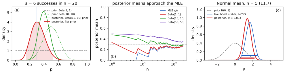
fig_11_s1. Download: PDF · SVGTwo further remarks complete the method. Posteriors can be updated as data arrive, and they depend on the data only through a sufficient statistic.
Filling the gap 11.6: updating one observation at a time, and sufficiency p. 177
(a) For iid data, the posterior after \(x_1,\dots,x_n\) is obtained by using the posterior after \(x_1,\dots,x_{n-1}\) as the prior for \(x_n\); in particular the order of the observations does not matter. (b) If \(T(\xn)\) is sufficient, in the sense that \(L_n(\th)=g(T(\xn),\th)h(\xn)\), the posterior depends on the data only through \(T(\xn)\).
Proof
(a) With proportionality constants that do not depend on \(\th\),
\[ f(\th\given x_1,\dots,x_n)\propto\Big[f(\th)\prod_{i=1}^{n-1}f(x_i\given\th)\Big]f(x_n\given\th)\propto f(\th\given x_1,\dots,x_{n-1})\,f(x_n\given\th). \]The product over \(i\) is symmetric in the \(x_i\), so the order is irrelevant. (b) In
\[ f(\th\given\xn)=\frac{g(T,\th)h(\xn)f(\th)}{\int g(T,\th')h(\xn)f(\th')\,\d\th'} \]the factor \(h(\xn)\) cancels. ∎
For the Beta–Bernoulli model, updating \(\Bet(\alpha,\beta)\) by one success gives \(\Bet(\alpha+1,\beta)\) and by one failure \(\Bet(\alpha,\beta+1)\); after all the data the result is \(\Bet(\alpha+s,\beta+n-s)\), which depends on the data only through \(s\). The credible-interval demo draws this sequence of posterior intervals; the biostatistics course does the same with a second series of data in Section 2.9.6.
11.3 Functions of Parameters
p. 180 To make inferences about \(\tau=g(\th)\), apply the method of Chapter 2 for the distribution of a function of a random variable (the three steps for a transformation) to the posterior: the posterior cdf of \(\tau\) is
\[ H(\tau\given\xn)=\P(g(\th)\le\tau\given\xn)=\int_Af(\th\given\xn)\,\d\th,\qquad A=\{\th:g(\th)\le\tau\}, \]and the posterior density is \(h(\tau\given\xn)=H'(\tau\given\xn)\).
Example 11.3 (the log-odds). p. 180 With Bernoulli data and the flat prior, \(p\given\xn\sim\Bet(s+1,n-s+1)\). For \(\psi=\log\{p/(1-p)\}\), whose inverse is \(p=e^\psi/(1+e^\psi)\),
\[ H(\psi\given\xn)=\P\Big(p\le\frac{e^\psi}{1+e^\psi}\,\Big|\,\xn\Big)=\int_0^{e^\psi/(1+e^\psi)}f(p\given\xn)\,\d p, \]and differentiating with the chain rule gives the density below. The book's last two lines contain a slip: the derivative of \(e^\psi/(1+e^\psi)\) is \(e^\psi/(1+e^\psi)^2\), not \(1/(1+e^\psi)^2\) (in the author's errata), so the exponents in the final formula are off by one.
Filling the gap 11.7: the posterior density of the log-odds, corrected p. 180, Example 11.3
With \(p\given\xn\sim\Bet(s+1,n-s+1)\), the posterior density of \(\psi=\logit p\) is, for \(\psi\in\R\),
\[ h(\psi\given\xn)=\frac{\Gamma(n+2)}{\Gamma(s+1)\Gamma(n-s+1)}\Big(\frac{e^\psi}{1+e^\psi}\Big)^{s+1}\Big(\frac1{1+e^\psi}\Big)^{n-s+1}, \]with posterior mean \(\E(\psi\given\xn)=\Psi(s+1)-\Psi(n-s+1)\), where \(\Psi=\Gamma'/\Gamma\) is the digamma function.
Proof
Write \(u(\psi)=e^\psi/(1+e^\psi)\); then \(1-u=1/(1+e^\psi)\) and \(u'(\psi)=e^\psi/(1+e^\psi)^2=u(1-u)\). Since \(u\) is increasing, \(H(\psi\given\xn)=F(u(\psi))\) with \(F\) the posterior cdf of \(p\), and by the chain rule \(h(\psi\given\xn)=f(u(\psi)\given\xn)\,u'(\psi)\). Substituting \(f(p\given\xn)\propto p^s(1-p)^{n-s}\) and \(u'=u(1-u)\) gives \(u^{s+1}(1-u)^{n-s+1}\) times the Beta constant: the display. (The book's version, with \(u'\) replaced by \((1-u)^2\), is proportional to \(u^s(1-u)^{n-s+2}\): the log-odds density of a \(\Bet(s,n-s+2)\) variable, which is shifted to the left; Figure 11.S2(a) shows both.)
For the mean, \(\psi=\log p-\log(1-p)\) and, for \(p\sim\Bet(a,b)\),
\[ \E\log p=\frac{\int_0^1\log p\;p^{a-1}(1-p)^{b-1}\,\d p}{B(a,b)}=\partial_a\log B(a,b)=\Psi(a)-\Psi(a+b), \]by differentiating the Beta integral under the integral sign (allowed since \(|\log p|\,p^{a-1}\) is integrable near 0 for \(a>0\)). Symmetrically \(\E\log(1-p)=\Psi(b)-\Psi(a+b)\). Subtracting, \(\E\psi=\Psi(a)-\Psi(b)\) with \(a=s+1\), \(b=n-s+1\). ∎
For \(s=6\), \(n=20\) the mean is \(\Psi(7)-\Psi(15)=-0.802\), close to but not equal to \(\logit\) of the posterior mean of \(p\), \(\logit(7/22)=-0.762\): posterior means are not equivariant under nonlinear maps, posterior quantiles are.
11.4 Simulation
pp. 180–181 Often the posterior is easier to sample than to integrate. Given draws \(\th_1,\dots,\th_B\sim f(\th\given\xn)\), a histogram approximates the posterior density, the average \(B^{-1}\sum_j\th_j\) approximates the posterior mean, and the sample quantiles \((\th_{\alpha/2},\th_{1-\alpha/2})\) approximate the \(1-\alpha\) posterior interval. For \(\tau=g(\th)\), the values \(\tau_j=g(\th_j)\) are draws from the posterior of \(\tau\), with no calculus at all. Chapter 24 of the book explains how to draw from a posterior that is known only up to its constant.
Example 11.4. p. 181 For Example 11.3: draw \(P_1,\dots,P_B\sim\Bet(s+1,n-s+1)\) and set \(\psi_i=\log\{P_i/(1-P_i)\}\). Figure 11.S2(a) shows the histogram of \(B=10\,000\) such values with the corrected density of Filling the gap 11.7; a Kolmogorov–Smirnov test on 200 000 draws accepts the corrected density and rejects the printed one decisively.
Filling the gap 11.8: why posterior simulation works, and how accurate it is p. 181
Let \(\th_1,\dots,\th_B\) be iid from the posterior (given \(\xn\)). (a) \(\tau_j=g(\th_j)\) are iid from the posterior of \(g(\th)\), for any measurable \(g\). (b) If \(\V(\th\given\xn)=v<\infty\), then \(B^{-1}\sum_j\th_j\to\bth\) almost surely, with Monte Carlo standard error \(\sqrt{v/B}\). (c) If the posterior cdf \(F\) is continuous and strictly increasing near its \(q\)-quantile \(t_q\), the sample \(q\)-quantile converges to \(t_q\) almost surely. (d) For increasing \(g\), the posterior \(q\)-quantile of \(g(\th)\) is \(g(t_q)\); so equal-tailed posterior intervals transform: the interval for \(g(\th)\) is \((g(a),g(b))\).
Proof
(a) \(\P(g(\th_j)\in A)=\P(\th_j\in g^{-1}(A))\) is the posterior probability of \(\{g(\th)\in A\}\), and functions of independent variables are independent. (b) The strong law of large numbers (Section 5.3) and \(\V(B^{-1}\sum_j\th_j)=v/B\). (c) Fix \(\epsilon>0\). By strict monotonicity, \(F(t_q-\epsilon)<q<F(t_q+\epsilon)\). The empirical cdf \(F_B(t)\) converges to \(F(t)\) almost surely at the two points \(t_q\pm\epsilon\) (strong law for indicators), so for all large \(B\), \(F_B(t_q-\epsilon)<q<F_B(t_q+\epsilon)\), which puts the sample \(q\)-quantile in \((t_q-\epsilon,t_q+\epsilon]\). (d) \(\P(g(\th)\le g(t)\given\xn)=\P(\th\le t\given\xn)\) for increasing \(g\). ∎
In Example 11.4 the posterior standard deviation of \(\psi\) is about 0.47, so with \(B=10\,000\) draws the posterior mean is estimated to within about \(\pm0.01\) (two Monte Carlo standard errors). Part (d) is why the exact interval for the log-odds is simply the logit of the interval for \(p\).
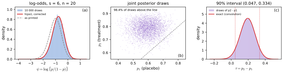
fig_11_s2. Download: PDF · SVG11.5 Large Sample Properties of Bayes' Procedures
p. 181 In both examples of Section 11.2 the posterior mean ended up close to the MLE. This is general.
Theorem 11.5 (the posterior is approximately Normal) p. 181
Let \(\hth\) be the MLE and \(\hse=1/\sqrt{nI(\hth)}\). Under regularity conditions, the posterior is approximately Normal with mean \(\hth\) and standard deviation \(\hse\); hence \(\bth\approx\hth\). If \(C_n=(\hth-z_{\alpha/2}\hse,\ \hth+z_{\alpha/2}\hse)\) is the asymptotic \(1-\alpha\) (Wald) confidence interval, then it is also an approximate \(1-\alpha\) posterior interval:
\[ \P(\th\in C_n\given\Xn)\to1-\alpha. \]There is also a Bayesian delta method: for \(\tau=g(\th)\), \(\tau\given\Xn\approx N(\widehat\tau,\widehat{\se}(\widehat\tau)^2)\) with \(\widehat\tau=g(\hth)\) and \(\widehat{\se}(\widehat\tau)=\hse\,|g'(\hth)|\).
The book gives a heuristic proof in its appendix (Section 11.11) and does not state the regularity conditions. The precise result is the Bernstein–von Mises theorem: the posterior and the Normal distribution are close in total variation, in probability under the true parameter. Here it is in one dimension with a complete proof.
Filling the gap 11.9: the Bernstein–von Mises theorem, with a proof p. 181, Theorem 11.5; p. 190, Appendix
Let \(X_1,X_2,\dots\) be iid \(f(x\given\th_0)\), with \(\th_0\) an interior point of an open interval \(\Theta\), and write \(\ell(\th;x)=\log f(x\given\th)\). Assume:
- (smoothness) \(\ell(\cdot;x)\) is three times continuously differentiable on a neighbourhood \(U=[\th_0-\delta_0,\th_0+\delta_0]\), with \(\sup_{\th\in U}|\ell'''(\th;x)|\le M(x)\) and \(\E_{\th_0}M(X)<\infty\); also \(\E_{\th_0}|\ell''(\th_0;X)|<\infty\);
- (information) \(I(\th_0)=-\E_{\th_0}\ell''(\th_0;X)\in(0,\infty)\);
- (MLE) with probability tending to 1 the MLE \(\hth\) exists, satisfies \(\ell_n'(\hth)=0\), and \(\hth\convp\th_0\);
- (separation) for every \(\delta>0\) there is \(\eta>0\) such that, with probability tending to 1, \(\ell_n(\th)-\ell_n(\th_0)\le-n\eta\) for all \(\th\) with \(|\th-\th_0|\ge\delta\);
- (prior) the prior is a proper density, continuous and positive at \(\th_0\).
Let \(\pi_n\) be the posterior density of \(h=\sqrt n(\th-\hth)\) and \(\phi_I\) the \(N(0,1/I(\th_0))\) density. Then
\[ \int_{\R}\big|\pi_n(h)-\phi_I(h)\big|\,\d h\convp0. \]Equivalently, \(\TV\big(\Pi(\cdot\given\Xn),\ N(\hth,1/(nI(\th_0)))\big)\convp0\), and the same holds with \(I(\th_0)\) replaced by \(I(\hth)\) if \(I\) is continuous at \(\th_0\), or by the observed information \(-\ell_n''(\hth)/n\).
Proof
Set-up. On the event (of probability tending to 1) where \(\hth\) exists, the posterior density of \(h\) is \(\pi_n(h)=g_n(h)/D_n\), with
\[ g_n(h)=f\big(\hth+h/\sqrt n\big)\exp\{\ell_n(\hth+h/\sqrt n)-\ell_n(\hth)\},\qquad D_n=\int g_n(h)\,\d h \](the change of variables \(\th=\hth+h/\sqrt n\) has Jacobian \(1/\sqrt n\), which cancels between numerator and denominator). Let \(g_0(h)=f(\th_0)e^{-I h^2/2}\) with \(I=I(\th_0)\), so that \(D_0=\int g_0=f(\th_0)\sqrt{2\pi/I}>0\) and \(\phi_I=g_0/D_0\). It suffices to prove \(\int|g_n-g_0|\convp0\). Indeed, then \(|D_n-D_0|\le\int|g_n-g_0|\convp0\), and
\[ \int\Big|\frac{g_n}{D_n}-\frac{g_0}{D_0}\Big|\le\frac{\int|g_n-g_0|}{D_n}+\frac{|D_0-D_n|}{D_n}\convp0. \]Taylor expansion. On the event \(\{|\hth-\th_0|\le\delta_0/2\}\), for \(|\th-\hth|\le\delta_0/2\) both points lie in \(U\), and since \(\ell_n'(\hth)=0\),
\[ \ell_n(\th)-\ell_n(\hth)=\tfrac12(\th-\hth)^2\ell_n''(\hth)+R,\qquad|R|\le\tfrac16|\th-\hth|^3\textstyle\sum_iM(X_i). \]With \(\th=\hth+h/\sqrt n\), \(J_n=-\ell_n''(\hth)/n\) and \(\overline M_n=n^{-1}\sum_iM(X_i)\), this reads \(\ell_n(\th)-\ell_n(\hth)=-\tfrac12h^2J_n+R_n(h)\) with \(|R_n(h)|\le|h|^3\overline M_n/(6\sqrt n)\). By the law of large numbers \(\overline M_n\to\mu_M=\E M(X)\), and \(J_n\convp I\): indeed \(|\ell''(\hth;x)-\ell''(\th_0;x)|\le M(x)|\hth-\th_0|\), so
\[ \Big|J_n-\Big(-\frac1n\sum_i\ell''(\th_0;X_i)\Big)\Big|\le\overline M_n|\hth-\th_0|\convp0, \]and the average converges to \(I\).
Three regions. Fix \(\epsilon>0\). Choose \(\delta\in(0,\delta_0/4]\) so small that \(2\delta\mu_M/3\le I/8\) and \(f(\th)\le2f(\th_0)\) for \(|\th-\th_0|\le3\delta\) (continuity of \(f\) at \(\th_0\)). Then choose \(K\) so large that \(3f(\th_0)\int_{|h|>K}e^{-Ih^2/8}\d h<\epsilon\). Work on the event \(E_n\) where \(|\hth-\th_0|\le\delta\), \(J_n\ge I/2\), \(\overline M_n\le2\mu_M\) and the separation inequality holds with this \(\delta\) and its \(\eta\); \(\P(E_n)\to1\).
(i) \(|h|\le K\). Here \(|R_n(h)|\le K^3\overline M_n/(6\sqrt n)\to0\) uniformly, \(\sup_{|h|\le K}|h^2(J_n-I)|\le K^2|J_n-I|\convp0\), and \(\sup_{|h|\le K}|f(\hth+h/\sqrt n)-f(\th_0)|\convp0\) by continuity of \(f\) at \(\th_0\) and consistency of \(\hth\). Hence \(\sup_{|h|\le K}|g_n(h)-g_0(h)|\convp0\), and the integral of \(|g_n-g_0|\) over \(|h|\le K\) is at most \(2K\) times this supremum.
(ii) \(K<|h|\le2\delta\sqrt n\). Here \(|\th-\hth|=|h|/\sqrt n\le2\delta\le\delta_0/2\), so the Taylor bound applies and
\[ |R_n(h)|\le h^2(2\delta)\overline M_n/6\le h^2\cdot2\delta\mu_M/3\le h^2I/8; \]with \(J_n\ge I/2\) the exponent is at most \(-h^2I/4+h^2I/8=-h^2I/8\). Also \(|\th-\th_0|\le3\delta\), so \(f(\th)\le2f(\th_0)\). Hence \(g_n(h)\le2f(\th_0)e^{-Ih^2/8}\), and with \(g_0\le f(\th_0)e^{-Ih^2/8}\) we get \(\int_{K<|h|\le2\delta\sqrt n}(g_n+g_0)<\epsilon\).
(iii) \(|h|>2\delta\sqrt n\). Here \(|\th-\hth|>2\delta\) and therefore \(|\th-\th_0|>\delta\). Since \(\ell_n(\hth)\ge\ell_n(\th_0)\) (the MLE maximises \(\ell_n\)), the separation inequality gives \(\ell_n(\th)-\ell_n(\hth)\le\ell_n(\th)-\ell_n(\th_0)\le-n\eta\) there, so
\[ \int_{|h|>2\delta\sqrt n}g_n(h)\,\d h=\sqrt n\int_{|\th-\hth|>2\delta}f(\th)e^{\ell_n(\th)-\ell_n(\hth)}\d\th\le\sqrt n\,e^{-n\eta}\int f(\th)\,\d\th=\sqrt n\,e^{-n\eta}\to0, \]using that the prior is proper; and \(\int_{|h|>2\delta\sqrt n}g_0\to0\).
Adding the three regions, \(\P(\int|g_n-g_0|>3\epsilon)\to0\) for every \(\epsilon\), which is the claim.
Other centrings and scales. Total variation is unchanged by the bijection \(h\mapsto\hth+h/\sqrt n\), which gives the statement about \(\Pi(\cdot\given\Xn)\). Two Normal laws with the same mean and variances \(\sigma_1^2,\sigma_2^2\) are at total variation distance at most \(\tfrac12\sqrt{2\,\mathrm{KL}}\) (Pinsker's inequality) with \(\mathrm{KL}=\tfrac12(r-1-\log r)\), \(r=\sigma_1^2/\sigma_2^2\), which tends to 0 when \(r\to1\); \(I(\hth)/I(\th_0)\convp1\) by continuity, and \(J_n/I\convp1\) was shown above. ∎
The assumptions deserve a word. Smoothness and positive information are what make the log-likelihood locally quadratic; the separation condition rules out a second, distant region of high likelihood (it holds, for instance, when \(\Theta\) is compact, the model is identifiable and \(\ell\) is continuous in \(\th\), by a uniform law of large numbers); the prior only needs to be continuous and positive at \(\th_0\): any such prior gives the same limit, which is why the prior "washes out". The same proof works in \(\R^k\) with \(I(\th_0)\) a positive definite matrix. Without the separation condition, or when the number of parameters grows with \(n\), the conclusion can fail (Example 11.9).
Filling the gap 11.10: posterior mean against MLE, posterior intervals, and the Bayesian delta method p. 181
Under the conditions of Filling the gap 11.9: (a) \(\P(\th\in C_n\given\Xn)\convp1-\alpha\) for the Wald interval \(C_n\); (b) if moreover the prior has a finite mean, \(\sqrt n(\bth-\hth)\convp0\), so the posterior mean and the MLE are asymptotically interchangeable; (c) if \(g\) is continuously differentiable with \(g'(\th_0)\ne0\), the posterior probability of \(g(\hth)\pm z_{\alpha/2}\hse|g'(\hth)|\) tends to \(1-\alpha\).
Proof
(a) Let \(Q_n=N(\hth,\hse^2)\). For any set \(A\), \(|\Pi(A\given\Xn)-Q_n(A)|\) is at most the total variation distance between \(\Pi(\cdot\given\Xn)\) and \(Q_n\), and \(Q_n(C_n)=1-\alpha\) exactly. The distance tends to 0 in probability by Filling the gap 11.9 (with \(I(\hth)\), assuming \(I\) continuous at \(\th_0\)).
(b) \(\sqrt n(\bth-\hth)=\int h\,\pi_n(h)\d h\) and \(\int h\,\phi_I(h)\d h=0\), so it suffices that \(\int|h|\,|\pi_n-\phi_I|\convp0\). Repeat the proof of Filling the gap 11.9 with the weight \(1+|h|\): in regions (i) and (ii) the bounds are multiplied by \(1+|h|\), still integrable against \(e^{-Ih^2/8}\); in region (iii) the bound becomes
\[ \sqrt n\,e^{-n\eta}\int(1+\sqrt n|\th-\hth|)f(\th)\,\d\th\le\sqrt n\,e^{-n\eta}\big(1+\sqrt n(\E_f|\th|+|\hth|)\big)\to0, \]which is where the finite prior mean is used.
(c) Let
\[ A_n=\big\{\th:|g(\th)-g(\hth)|\le z_{\alpha/2}\,\hse\,|g'(\hth)|\big\}. \]As in (a), \(|\Pi(A_n\given\Xn)-Q_n(A_n)|\to0\) in probability. Under \(Q_n\), \(\th=\hth+\hse Z\) with \(Z\sim N(0,1)\), and by the mean value theorem \(g(\th)-g(\hth)=g'(\xi)\hse Z\) for some \(\xi\) between \(\hth\) and \(\th\). Since \(\hse\to0\) and \(g'\) is continuous, \(g'(\xi)/g'(\hth)\to1\) in \(Q_n\)-probability, so
\[ Q_n(A_n)=\P\big(|Z\,g'(\xi)/g'(\hth)|\le z_{\alpha/2}\big)\to\P(|Z|\le z_{\alpha/2})=1-\alpha \]by Slutsky's theorem (Theorem 5.5). This is the frequentist delta method (Theorem 5.13) applied to the Normal approximation of the posterior. ∎
How fast? The distance in Filling the gap 11.9 is typically of order \(n^{-1/2}\): the posterior is skewed by the third derivative of \(\ell\) and shifted by the prior, both effects of relative size \(1/\sqrt n\). For the exponential model of the nerve data with the flat prior on the rate, the total variation distance is 0.084 at \(n=10\), 0.027 at \(n=100\) and 0.0094 at \(n=799\) (slope \(-0.50\) on log scales), and the posterior probability of the 95% Wald interval is 0.927, 0.948 and 0.950 (Figure 11.S3). The log scale does not reduce the distance (0.088, 0.028, 0.0099) but it moves the posterior probability of the Wald interval for \(\log\lambda\) closer to 95% at small \(n\) (0.955 at \(n=10\)).
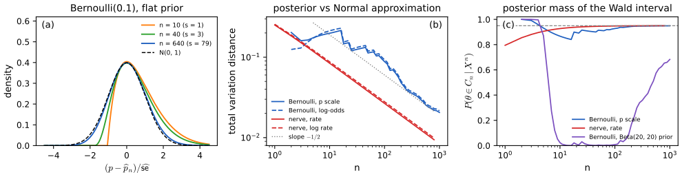
fig_11_s3. Download: PDF · SVGSee also (companion courses): the Laplace approximation, which centres the same Normal at the posterior mode with the curvature of the log-posterior, in Section 4.4 of Bayesian and Probabilistic Machine Learning; the bootstrap as an approximate posterior in Section 8.4 of Statistical Learning: Theory and Methods.
11.6 Flat Priors, Improper Priors, and "Noninformative" Priors
pp. 181–182 Where does the prior come from? Subjectivists answer: from your honest opinion before the data. That is feasible in small problems but impractical with many parameters, and it sits uneasily with the aim of objective scientific inference. The alternative is a "noninformative" prior, and the obvious candidate is a flat one, \(f(\th)\propto\) constant. In the Bernoulli example \(f(p)=1\) gave the sensible \(\Bet(s+1,n-s+1)\). Two problems arise.
Definition 11.C (improper prior) p. 182
A non-negative function \(f\) with \(\int f(\th)\d\th=\infty\), used as a prior through (11.2), is an improper prior. The formal posterior \(L_n(\th)f(\th)/\int L_n f\) is legitimate whenever \(0<\int L_n(\th)f(\th)\d\th<\infty\).
Improper priors. For \(X_1,\dots,X_n\sim N(\th,\sigma^2)\) with \(\sigma\) known and the flat prior \(f(\th)\propto c\), the formal posterior is \(f(\th\given\xn)\propto L_n(\th)f(\th)\propto L_n(\th)\) (the book writes \(f(\th)\) on the left, a slip: it is the posterior), that is \(\th\given\xn\sim N(\overline x,\sigma^2/n)\), and the Bayesian point and interval estimates coincide with the frequentist ones. Improper priors are acceptable as long as the posterior is a proper distribution.
Filling the gap 11.11: when an improper prior gives a proper posterior p. 182
(a) Normal mean, flat prior:
\[ \int L_n(\th)\,\d\th=(2\pi\sigma^2)^{-n/2}e^{-\sum_i(x_i-\overline x)^2/(2\sigma^2)}\sqrt{2\pi\sigma^2/n}<\infty, \]so the posterior \(N(\overline x,\sigma^2/n)\) is proper for every data set, and the posterior interval \(\overline x\pm z_{\alpha/2}\sigma/\sqrt n\) has frequentist coverage exactly \(1-\alpha\) for every \(\th\). (b) Bernoulli with the improper prior \(f(p)=1/\{p(1-p)\}\) (which is flat on the log-odds, Filling the gap 11.12): the posterior \(\Bet(s,n-s)\) is proper if and only if \(0<s<n\). (c) The scaling constant of an improper prior is arbitrary, and it cancels in (11.2); this is exactly what goes wrong in testing (Filling the gap 11.15).
Proof
(a) By the decomposition \(\sum_i(x_i-\th)^2=\sum_i(x_i-\overline x)^2+n(\th-\overline x)^2\) (as in Filling the gap 11.5), \(L_n(\th)\) is a constant times the \(N(\overline x,\sigma^2/n)\) density in \(\th\); its integral is the stated finite number. The interval is \(\overline X\pm z_{\alpha/2}\sigma/\sqrt n\), and \(\P_\th(|\overline X-\th|<z_{\alpha/2}\sigma/\sqrt n)=1-\alpha\) since \(\sqrt n(\overline X-\th)/\sigma\sim N(0,1)\) under \(\P_\th\).
(b) \(L_n(p)/\{p(1-p)\}=p^{s-1}(1-p)^{n-s-1}\), and \(\int_0^1p^{a-1}(1-p)^{b-1}\d p\) is finite if and only if \(a>0\) and \(b>0\) (near 0 the integrand behaves like \(p^{a-1}\), integrable iff \(a>0\); similarly near 1). So the posterior exists iff \(s\ge1\) and \(n-s\ge1\).
(c) Replacing \(f\) by \(kf\) multiplies numerator and denominator of (11.2) by \(k\). ∎
Part (b) is a real hazard: after 10 failures and no success, the prior that is "flat on the log-odds" gives no posterior at all; the Jeffreys-prior demo shows the case. The flat prior on \(p\) and Jeffreys' prior both give proper posteriors for every data set.
Flat priors are not invariant. p. 182 Take \(X\sim\Bern(p)\) and \(f(p)=1\), meant to express ignorance about \(p\). The log-odds \(\psi=\log\{p/(1-p)\}\) then has the density \(f_\Psi(\psi)=e^\psi/(1+e^\psi)^2\), which is not flat. But ignorance about \(p\) is ignorance about \(\psi\), so a flat prior on \(\psi\) would seem equally justified, and the two choices contradict each other. "Flat" is not a well-defined notion: it depends on the parametrisation.
Filling the gap 11.12: what a flat prior on one scale is on another p. 182
If \(\phi=g(\th)\) with \(g\) smooth and strictly monotone, a prior density \(f_\Theta\) for \(\th\) is the density \(f_\Phi(\phi)=f_\Theta(g^{-1}(\phi))\,|\d g^{-1}(\phi)/\d\phi|\) for \(\phi\); equivalently, a prior flat in \(\phi\) is the prior \(f_\Theta(\th)\propto|g'(\th)|\) for \(\th\). In particular, flat on \(p\) is the logistic density \(e^\psi/(1+e^\psi)^2\) on \(\psi=\logit p\), and flat on \(\psi\) is the improper prior \(1/\{p(1-p)\}\) on \(p\).
Proof
This is the transformation formula for densities (Result 2.17): for increasing \(g\), \(\P(\Phi\le\phi)=\P(\Theta\le g^{-1}(\phi))\), and differentiating gives \(f_\Theta(g^{-1}(\phi))\,(g^{-1})'(\phi)\); for decreasing \(g\) the sign flips, hence the absolute value. For the flat prior on \(p\) and \(\psi=\logit p\): \(g^{-1}(\psi)=e^\psi/(1+e^\psi)\) with derivative \(e^\psi/(1+e^\psi)^2\), and \(f_\Theta\equiv1\). Conversely, \(f_\Phi\equiv1\) corresponds to \(f_\Theta(p)=|g'(p)|=1/\{p(1-p)\}\). ∎
The logistic density integrates to 1 and is symmetric about 0 with variance \(\pi^2/3\): flat on \(p\) says that the log-odds is probably between \(-3\) and 3 (Figure 11.S4(a)). The prior \(1/\{p(1-p)\}\) piles infinite mass near 0 and 1. Which of these is "noninformative"? Neither choice is privileged; that is the point. The same mechanism (the Jacobian) is explained for machine-learning readers in Section 2.4 of Foundations of Deep Learning.
Definition 11.D (Jeffreys' prior) pp. 182–183
For a one-parameter model, Jeffreys' prior is \(f(\th)\propto I(\th)^{1/2}\), with \(I(\th)\) the Fisher information. For \(\th=(\th_1,\dots,\th_k)\) it is \(f(\th)\propto\sqrt{\det I(\th)}\), with \(I(\th)\) the Fisher information matrix.
The book says this rule "turns out to be transformation invariant" without explaining what that means or why. Here is both.
Filling the gap 11.13: Jeffreys' prior is invariant, and what it is in standard models pp. 182–183
(a) Invariance. Let \(\phi=g(\th)\) with \(g\) a smooth bijection with nonzero derivative. Applying Jeffreys' rule in the \(\phi\) parametrisation, \(f_\Phi(\phi)\propto\sqrt{I_\Phi(\phi)}\), and carrying the result back to \(\th\) with the Jacobian gives \(\sqrt{I_\Theta(\th)}\): the rule produces the same beliefs whichever parametrisation it is applied in. The same holds in \(\R^k\) with determinants. (b) Examples. Bernoulli: \(\Bet(1/2,1/2)\). Poisson: \(\lambda^{-1/2}\) (improper). \(N(\mu,\sigma^2)\) with \(\sigma\) known: flat in \(\mu\). Scale \(\sigma\) with \(\mu\) known: \(1/\sigma\). Both \((\mu,\sigma)\): \(1/\sigma^2\). (c) Flat in the variance-stabilising scale. If \(\phi=\int^\th\sqrt{I(t)}\d t\), then \(I_\Phi\equiv1\) and Jeffreys' prior is flat in \(\phi\); for the Bernoulli, \(\phi=2\arcsin\sqrt p\).
Proof
(a) Write \(\th=\th(\phi)=g^{-1}(\phi)\). The score in the new parametrisation is, by the chain rule, \(\partial_\phi\log f(X\given\th(\phi))=\th'(\phi)\,\partial_\th\log f(X\given\th)\), so \(I_\Phi(\phi)=\E[(\partial_\phi\log f)^2]=\th'(\phi)^2I_\Theta(\th(\phi))\). Hence \(\sqrt{I_\Phi(\phi)}=|\th'(\phi)|\sqrt{I_\Theta(\th(\phi))}\). Carrying this density back to \(\th\) multiplies by \(|\d\phi/\d\th|=1/|\th'(\phi)|\) (Filling the gap 11.12), leaving \(\sqrt{I_\Theta(\th)}\). In \(\R^k\), with \(J=\partial\th/\partial\phi\), the score transforms as \(J^\T\nabla_\th\log f\), so \(I_\Phi=J^\T I_\Theta J\) and \(\sqrt{\det I_\Phi}=|\det J|\sqrt{\det I_\Theta}\); the Jacobian of the change of variables is again \(|\det J|\).
(b) Bernoulli: \(\partial_p\log f=x/p-(1-x)/(1-p)\), whose second moment is \(p\cdot p^{-2}+(1-p)(1-p)^{-2}=1/\{p(1-p)\}\); so \(f(p)\propto p^{-1/2}(1-p)^{-1/2}\), the \(\Bet(1/2,1/2)\) density (proper, with constant \(1/\pi\)). Poisson: the score is \(x/\lambda-1\), with variance \(\V(X)/\lambda^2=1/\lambda\); so \(f\propto\lambda^{-1/2}\), and \(\int_0^\infty\lambda^{-1/2}\d\lambda=\infty\). Normal mean: the score is \((x-\mu)/\sigma^2\), with variance \(1/\sigma^2\), constant in \(\mu\). Normal scale: the score in \(\sigma\) is \(-1/\sigma+(x-\mu)^2/\sigma^3\), with variance \(\V((x-\mu)^2)/\sigma^6=2\sigma^4/\sigma^6=2/\sigma^2\), so \(f\propto1/\sigma\). Both: the information matrix is \(\mathrm{diag}(1/\sigma^2,2/\sigma^2)\) (the off-diagonal term \(\E[(X-\mu)^3]/\sigma^5-\E[X-\mu]/\sigma^3\) vanishes), with determinant \(2/\sigma^4\), so \(f\propto1/\sigma^2\). This differs from the product of the two one-parameter answers, \(1/\sigma\); many authors prefer the latter (Kass and Wasserman 1996 discuss why).
(c) \(\phi'(\th)=\sqrt{I(\th)}\), so by the formula in (a) \(I_\Phi=I_\Theta/\phi'(\th)^2=1\). For the Bernoulli, \(\int\{p(1-p)\}^{-1/2}\d p=2\arcsin\sqrt p\). ∎
Two remarks. First, "variance-stabilising" is meant literally: by the delta method, \(\sqrt n(\phi(\hth)-\phi(\th))\convd N(0,1)\) whatever \(\th\), so Jeffreys' prior is the flat prior in the one scale where the data are equally informative everywhere. Second, the book calls \(\Bet(1/2,1/2)\) "very close to a uniform density". It is U-shaped and unbounded at both ends; it crosses 1 at \(p=\tfrac12(1\pm\sqrt{1-4/\pi^2})\), that is at 0.114 and 0.886, and its total variation distance from the uniform is
\[ \TV=(p_2-p_1)-\frac2\pi\big(\arcsin\sqrt{p_2}-\arcsin\sqrt{p_1}\big)=0.2105. \]What is true is that the two lead to similar posteriors once \(s\) and \(n-s\) are both moderately large (each adds less than one pseudo-observation). The invariance argument is also given in Filling the gap 2.6 of Bayesian and Probabilistic Machine Learning.
Example 11.6 (Jeffreys' prior for a proportion). p. 183 For the \(\Bern(p)\) model \(I(p)=1/\{p(1-p)\}\), so Jeffreys' rule gives \(f(p)\propto p^{-1/2}(1-p)^{-1/2}\), the \(\Bet(1/2,1/2)\) density, and the posterior is \(\Bet(s+1/2,n-s+1/2)\). In the multiparameter case the rule uses \(\sqrt{\det I(\th)}\).
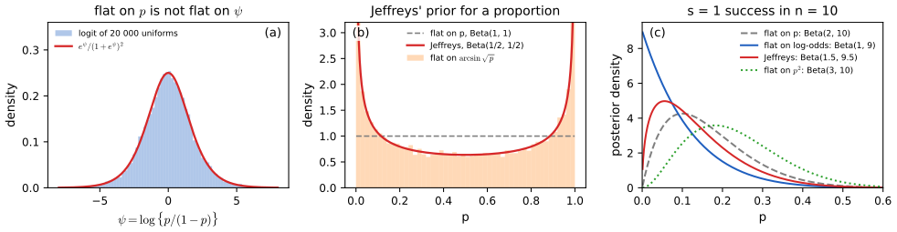
fig_11_s4. Download: PDF · SVGSee also (companion courses): noninformative priors for location and scale parameters in Section 2.4.3 of Bayesian and Probabilistic Machine Learning.
11.7 Multiparameter Problems
pp. 183–184 For \(\th=(\th_1,\dots,\th_p)\) the posterior is still
\[ f(\th\given\xn)\propto L_n(\th)f(\th). \tag{11.8} \]Inference about one coordinate uses its marginal posterior
\[ f(\th_1\given\xn)=\int\cdots\int f(\th_1,\dots,\th_p\given\xn)\,\d\th_2\cdots\d\th_p. \tag{11.9} \]The integral is often intractable, but simulation avoids it: draw \(\th^1,\dots,\th^B\) from the joint posterior (superscripts index the draws) and keep the first coordinates \(\th^1_1,\dots,\th^B_1\); they are a sample from (11.9).
Example 11.7 (comparing two binomials). pp. 183–184 Of \(n_1\) control patients \(X_1\) survive and of \(n_2\) treated patients \(X_2\) survive, with \(X_1\sim\Bin(n_1,p_1)\) and \(X_2\sim\Bin(n_2,p_2)\) independent; the target is \(\tau=p_2-p_1\). With the flat prior \(f(p_1,p_2)=1\) on the unit square,
\[ f(p_1,p_2\given x_1,x_2)\propto p_1^{x_1}(1-p_1)^{n_1-x_1}\,p_2^{x_2}(1-p_2)^{n_2-x_2}=f(p_1\given x_1)f(p_2\given x_2), \]so \(p_1\) and \(p_2\) are independent a posteriori, with \(p_j\given x_j\sim\Bet(x_j+1,n_j-x_j+1)\). Drawing \(P_{1,b}\) and \(P_{2,b}\) independently from these and setting \(\tau_b=P_{2,b}-P_{1,b}\) gives a sample from \(f(\tau\given x_1,x_2)\).
Filling the gap 11.14: marginals by projection, posterior independence, and the exact density of \(p_2-p_1\) pp. 183–184
(a) If \(\th^b\) is drawn from the joint posterior, its first coordinate is a draw from (11.9). (b) In Example 11.7 the joint posterior factorises because the likelihood and the prior both factorise. (c) The posterior density of \(\tau=p_2-p_1\) is the convolution
\[ f(\tau\given x_1,x_2)=\int_{\max(0,-\tau)}^{\min(1,1-\tau)}f(p\given x_1)\,f(p+\tau\given x_2)\,\d p,\qquad-1<\tau<1, \]and its mean is \(\E(\tau\given x_1,x_2)=\frac{x_2+1}{n_2+2}-\frac{x_1+1}{n_1+2}\).
Proof
(a) By Fubini's theorem,
\[ \P(\th_1\in A)=\P(\th\in A\times\R^{p-1})=\int_A\Big[\int f(\th_1,\th_2,\dots\given\xn)\,\d\th_2\cdots\d\th_p\Big]\d\th_1, \]which is (11.9). (b) If \(f(\th)=f_1(\th_1)f_2(\th_2)\) and \(L(\th)=L_1(\th_1)L_2(\th_2)\), then \(f(\th\given x)\propto[L_1f_1](\th_1)\cdot[L_2f_2](\th_2)\), and a joint density that is a product of a function of \(\th_1\) and a function of \(\th_2\) on a product set means independence, each factor normalised being the marginal. (c) For independent \(P_1,P_2\) with densities \(f_1,f_2\), \(\P(P_2-P_1\le t)=\int f_1(p)\P(P_2\le p+t)\d p\); differentiate in \(t\) under the integral (the integrand is bounded by \(f_1(p)\sup f_2\), and \(\sup f_2<\infty\) for these Betas) to get \(\int f_1(p)f_2(p+t)\d p\), with \(p\) restricted to where both arguments lie in \((0,1)\). The mean is the difference of the two Beta means. ∎
With the data of Exercise 11.4 (30/50 and 40/50) the exact posterior mean of \(\tau\) is \(41/52-31/52=0.192\) and \(\P(\tau>0\given\text{data})=0.985\) by numerical integration of the convolution, both reproduced by 100 000 simulated differences (Figure 11.S2(b, c)).
11.8 Bayesian Testing
pp. 184–185 To test \(H_0:\th=\th_0\) against \(H_1:\th\ne\th_0\) the Bayesian puts prior probabilities on the hypotheses, typically \(\P(H_0)=\P(H_1)=1/2\), and a prior density \(f(\th)\) for \(\th\) under \(H_1\). Bayes' theorem then gives
\[ \P(H_0\given\Xn=\xn)=\frac{\tfrac12f(\xn\given\th_0)}{\tfrac12f(\xn\given\th_0)+\tfrac12\int f(\xn\given\th)f(\th)\d\th}=\frac{L(\th_0)}{L(\th_0)+\int L(\th)f(\th)\,\d\th}. \]In estimation the prior mattered little for large \(n\); in testing it matters a great deal. Improper priors cannot be used, because the arbitrary constant in \(f\) no longer cancels. And since \(0\le\int L(\th)f(\th)\d\th\le L(\hth)\), there is a prior-free lower bound
\[ \frac{L(\th_0)}{L(\th_0)+L(\hth)}\le\P(H_0\given\Xn=\xn)\le1. \]Filling the gap 11.15: the posterior probability of a point null, Bayes factors, and the Jeffreys–Lindley paradox pp. 184–185; Exercise 11.8
(a) The formula above is Bayes' theorem for the mixed prior \(\tfrac12\delta_{\th_0}+\tfrac12f\). Its odds form is posterior odds = prior odds \(\times\) Bayes factor, with \(B_{01}=L(\th_0)/\int L(\th)f(\th)\d\th\). (b) With an improper \(f\), \(\P(H_0\given\xn)\) can be made any number in \((0,1)\). (c) The lower bound holds for every proper \(f\). (d) For \(X_1,\dots,X_n\sim N(\mu,1)\), \(H_0:\mu=0\), \(\mu\sim N(0,b^2)\) under \(H_1\), and \(z=\sqrt n\,\overline x\) (the Wald statistic),
\[ \P(H_0\given\xn)=\Big[1+\frac1{\sqrt{1+nb^2}}\exp\Big(\frac{z^2}2\cdot\frac{nb^2}{1+nb^2}\Big)\Big]^{-1}. \](e) For fixed \(z\) (fixed p-value) and \(n\to\infty\), \(\P(H_0\given\xn)\to1\): a result that is "significant at 5%" can be strong evidence for \(H_0\). (f) Over all \(b\) (with \(n=1\), \(x=z\), \(|z|>1\)), the smallest value is \(1/(1+e^{(z^2-1)/2}/|z|)\), attained at \(b^2=z^2-1\); the prior-free bound is \(1/(1+e^{z^2/2})\).
Proof
(a) The prior puts mass \(\tfrac12\) on \(\{\th_0\}\) and spreads \(\tfrac12\) with density \(f\) elsewhere; the marginal density of the data is \(\tfrac12L(\th_0)+\tfrac12\int Lf\), and \(\P(H_0\given\xn)\) is the \(H_0\) part divided by the total (Bayes' theorem with a partition into \(H_0\) and \(H_1\)). Dividing \(\P(H_0\given\xn)\) by \(\P(H_1\given\xn)\) gives \(\frac{\P(H_0)}{\P(H_1)}B_{01}\).
(b) Replacing \(f\) by \(kf\) divides \(B_{01}\) by \(k\), and \(k>0\) is arbitrary for an improper prior; writing \(B^{(1)}_{01}\) for the Bayes factor with \(k=1\), \(\P(H_0\given\xn)=1/(1+k/B^{(1)}_{01})\), which ranges over all of \((0,1)\) as \(k\) ranges over \((0,\infty)\).
(c) \(\int L(\th)f(\th)\d\th\le\sup_\th L(\th)\int f=L(\hth)\), and \(x\mapsto a/(a+x)\) is decreasing.
(d) \(\overline X\) is sufficient, so the likelihood ratio is that of \(\overline X\) (Filling the gap 11.6). Under \(H_0\), \(\overline X\sim N(0,1/n)\); under \(H_1\), \(\overline X=\mu+\epsilon\) with \(\mu\sim N(0,b^2)\) and \(\epsilon\sim N(0,1/n)\) independent, so marginally \(\overline X\sim N(0,b^2+1/n)\). The ratio of the two densities at \(\overline x\) is
\[ B_{01}=\frac{\sqrt{n}\,e^{-n\overline x^2/2}}{(b^2+1/n)^{-1/2}e^{-\overline x^2/(2(b^2+1/n))}}=\sqrt{1+nb^2}\,\exp\Big(-\frac{z^2}2\Big(1-\frac1{1+nb^2}\Big)\Big), \]and \(\P(H_0\given\xn)=1/(1+1/B_{01})\), which is the display.
(e) The term added to 1 is at most \((nb^2)^{-1/2}e^{z^2/2}\to0\).
(f) With \(n=1\) and \(v=1+b^2\ge1\), \(1/B_{01}=v^{-1/2}e^{(z^2/2)(1-1/v)}\). Its logarithm \(-\tfrac12\log v+\tfrac{z^2}2(1-1/v)\) has derivative \(-\tfrac1{2v}+\tfrac{z^2}{2v^2}\), positive for \(v<z^2\) and negative after, so the maximum of \(1/B_{01}\) (the minimum of \(\P(H_0\given x)\)) is at \(v=z^2\), with value \(e^{(z^2-1)/2}/|z|\). The prior-free bound: \(L(\th_0)/L(\hth)=e^{-z^2/2}\) since \(\hth=x\). ∎
Numbers. With \(x=1.96\) (two-sided p-value 0.05) and \(n=1\): \(\P(H_0\given x)=0.432\), 0.351, 0.360 and 0.600 for \(b=0.5\), 1, 3 and 10; the minimum over Normal priors is 0.321 (at \(b=1.69\)) and the bound over all priors is 0.128. With \(x=2.576\) (p-value 0.01) the two minima are 0.133 and 0.035. Keeping \(z=1.96\) and \(b=1\) while \(n\) grows, \(\P(H_0\given\xn)\) is 0.35 at \(n=1\), 0.60 at \(n=100\), 0.94 at \(n=10^4\) and 0.993 at \(n=10^6\) (Figure 11.S5). The disagreement was pointed out by Lindley (1957); the lower bounds are in Berger and Sellke (1987). Bayes factors as a tool for model comparison are developed in Section 3.4 of Bayesian and Probabilistic Machine Learning.
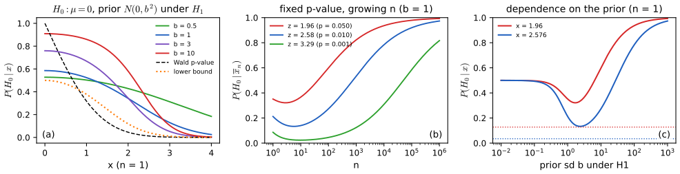
fig_11_s5. Download: PDF · SVG11.9 Strengths and Weaknesses of Bayesian Inference
pp. 185–189 Bayes' theorem is a principled way to combine prior information with data, and it is natural when such information exists. It also lets us say "\(\th\) is in \(C_n\) with probability 95%", which a confidence interval does not: the 95% of a confidence interval is a property of the procedure, a probability statement about \(C_n\) and not about \(\th\). The book is careful to add that psychological appeal is not a scientific argument. In parametric models with large samples the two approaches give approximately the same answers (Theorem 11.5); in general they need not. Three examples follow: the first shows the appeal, the second and third show failures.
Example 11.8 (Example 6.14 revisited). pp. 185–186 Let \(\th\) be a fixed unknown real number (the book again prints "known", as in Example 6.14; see the notes on the book), let \(X_1,X_2\) be independent with \(\P(X_i=1)=\P(X_i=-1)=1/2\), and observe only \(Y_i=\th+X_i\). The set \(C=\{Y_1-1\}\) if \(Y_1=Y_2\) and \(C=\{(Y_1+Y_2)/2\}\) if \(Y_1\ne Y_2\) is a 75% confidence set: \(\P_\th(\th\in C)=3/4\) for every \(\th\) (Filling the gap 6.10). After observing \(Y_1=15\), \(Y_2=17\), \(C=\{16\}\) and we know for certain that \(\th=16\). The Bayesian answer, for an integer \(\th\) and any prior mass function with \(f(\th)>0\) for every integer: the likelihood is \(1/4\) at \(\th=16\) and 0 elsewhere, so \(\P(\th=16\given Y=(15,17))=1\). Calling \(\{16\}\) a 75% confidence set is not wrong, but it is not a probability statement about \(\th\).
Filling the gap 11.16: the Bayesian analysis of Example 11.8 in both cases pp. 185–186
Let \(f\) be a prior mass function on the integers with \(f(\th)>0\) everywhere. (a) If \(Y_1\ne Y_2\) the posterior is a point mass at \((Y_1+Y_2)/2\). (b) If \(Y_1=Y_2=y\) the posterior puts mass \(f(y-1)/\{f(y-1)+f(y+1)\}\) on \(y-1\) and the rest on \(y+1\). (c) The confidence set \(C\) traps \(\th\) with conditional frequency 1 given \(Y_1\ne Y_2\) and \(1/2\) given \(Y_1=Y_2\); its 75% is the average of the two.
Proof
The four equally likely values of \((X_1,X_2)\) give \(L(\th)=\P(Y=(y_1,y_2)\given\th)=\tfrac14\) if \(\{y_1-\th,y_2-\th\}\subset\{-1,1\}\) is consistent with some \((x_1,x_2)\), and 0 otherwise. (a) If \(y_1\ne y_2\), then \(\{y_1,y_2\}=\{\th-1,\th+1\}\), which forces \(\th=(y_1+y_2)/2\): a single \(\th\) has positive likelihood, and the posterior is the point mass there whatever the prior. (b) If \(y_1=y_2=y\), the likelihood is \(\tfrac14\) at both \(\th=y-1\) and \(\th=y+1\); Bayes' theorem gives posterior masses proportional to \(f(y-1)\) and \(f(y+1)\). (c) Given \(Y_1\ne Y_2\) (probability 1/2), \(C\) is the correct value. Given \(Y_1=Y_2\), which happens when \(X_1=X_2=1\) or \(X_1=X_2=-1\) with conditional probability 1/2 each, \(C=\{Y_1-1\}\) is correct only in the first case. So \(\P_\th(\th\in C)=\tfrac12\cdot1+\tfrac12\cdot\tfrac12=\tfrac34\). ∎
So the posterior reports exactly the conditional information that the 75% averages away: certainty in half of the cases, a prior-dependent coin flip in the other half. With a flat prior on the integers (improper, but the posterior is proper) the second case gives \(\tfrac12\) and \(\tfrac12\), which is also the conditional frequency of being right.
Example 11.9 (a simplified version of the example of Robins and Ritov 1997). pp. 186–188 Let \(B\) be finite but huge (the book suggests \(100^{100}\)), much larger than any feasible \(n\). The unknown parameter is \(\th=(\th_1,\dots,\th_B)\in[0,1]^B\), and \(\xi=(\xi_1,\dots,\xi_B)\) is a vector of known numbers with \(0<\delta\le\xi_j\le1-\delta\). Each observation \((X_i,R_i,Y_i)\) is drawn as follows: \(X_i\) is uniform on \(\{1,\dots,B\}\); \(R_i\sim\Bern(\xi_{X_i})\); if \(R_i=1\) then \(Y_i\sim\Bern(\th_{X_i})\) is observed, and if \(R_i=0\) it is missing. The target is
\[ \psi=\P(Y_i=1)=\sum_{j=1}^B\P(Y_i=1\given X_i=j)\P(X_i=j)=\frac1B\sum_{j=1}^B\th_j. \]The likelihood of one observation is
\[ f(X_i)f(R_i\given X_i)f(Y_i\given X_i)^{R_i}=\frac1B\,\xi_{X_i}^{R_i}(1-\xi_{X_i})^{1-R_i}\,\th_{X_i}^{Y_iR_i}(1-\th_{X_i})^{(1-Y_i)R_i}, \]and dropping the known factors,
\[ \ell(\th)=\sum_{i=1}^nY_iR_i\log\th_{X_i}+(1-Y_i)R_i\log(1-\th_{X_i})=\sum_{j=1}^Bn_j\log\th_j+\sum_{j=1}^Bm_j\log(1-\th_j), \]with \(n_j=\#\{i:Y_i=1,R_i=1,X_i=j\}\) and \(m_j=\#\{i:Y_i=0,R_i=1,X_i=j\}\). Since \(B\gg n\), \(n_j=m_j=0\) for almost every \(j\): the MLE of most \(\th_j\) is undefined, and for most \(j\) the posterior of \(\th_j\) is its prior. Hence \(f(\psi\given\text{data})\approx f(\psi)\): in a Bayesian analysis the data say little about \(\psi\). The frequentist Horvitz–Thompson estimator
\[ \widehat\psi=\frac1n\sum_{i=1}^n\frac{R_iY_i}{\xi_{X_i}} \tag{11.10} \]satisfies (Exercise 11.7)
\[ \E(\widehat\psi)=\psi,\qquad\V(\widehat\psi)\le\frac1{n\delta^2}, \tag{11.11} \]so its mean squared error is of order \(1/n\) however large \(B\) is. It cannot come from a likelihood-based method, because the \(\xi_{X_i}\) it uses drop out of the likelihood. Bayesian methods are tied to the likelihood, and in high-dimensional and nonparametric problems the likelihood may not support accurate inference.
Filling the gap 11.17: what a Bayesian gets in Example 11.9, and why Horvitz–Thompson works pp. 186–188, (11.10)–(11.11); Exercise 11.7
(a) Independent priors. If the \(\th_j\) are independent \(\Unif(0,1)\) a priori, \(|\E(\psi\given\text{data})-\tfrac12|\le n/B\), whatever the data. (b) An exchangeable prior. If, given \(\mu\sim\Unif(0,1)\), the \(\th_j\) are iid \(\Bet(\kappa\mu,\kappa(1-\mu))\) for some \(\kappa>0\), and the observed cells \(X_i\) (with \(R_i=1\)) are distinct, then
\[ \Big|\E(\psi\given\text{data})-\frac{1+\sum_iR_iY_i}{2+\sum_iR_i}\Big|\le\frac nB,\qquad\frac{1+\sum_iR_iY_i}{2+\sum_iR_i}\to\frac{\E(\xi_X\th_X)}{\E(\xi_X)}=\psi+\frac{\Cov(\xi_X,\th_X)}{\E(\xi_X)} \]almost surely as \(n\to\infty\) (with \(X\) uniform on the cells). This is \(\psi\) only if the response probabilities \(\xi\) and the outcomes \(\th\) are uncorrelated across cells. (c) Horvitz–Thompson. \(\E\widehat\psi=\psi\) and \(\V(\widehat\psi)=\frac1n\big(\E[\th_X/\xi_X]-\psi^2\big)\le\frac1{n\delta}\le\frac1{n\delta^2}\).
Proof
(a) The likelihood factorises over cells, so with independent priors the posterior makes the \(\th_j\) independent, \(\th_j\given\text{data}\sim\Bet(1+n_j,1+m_j)\). At most \(n\) cells are observed; the others keep the prior mean \(\tfrac12\). So \(\E(\psi\given\text{data})=\frac1B\sum_j\E(\th_j\given\text{data})\) differs from \(\tfrac12\) by at most \(\frac1B\cdot n\cdot\tfrac12\le n/B\).
(b) Given \(\mu\), distinct observed cells have independent \(\th\)'s, each with mean \(\mu\); integrating \(\th_{X_i}\) out, the observed \(Y_i\) are independent \(\Bern(\mu)\) given \(\mu\), whatever \(\kappa\). (The \(X_i\) and \(R_i\) have distributions free of \(\th\) and \(\mu\), so they contribute only constants.) The posterior of \(\mu\) is therefore \(\Bet(1+\sum_iR_iY_i,1+\sum_iR_i(1-Y_i))\), with mean \((1+\sum R_iY_i)/(2+\sum R_i)\). For an unobserved cell, conditioning first on \(\mu\) gives \(\E(\th_j\given\text{data})=\E(\mu\given\text{data})\), so as in (a) \(\E(\psi\given\text{data})\) differs from \(\E(\mu\given\text{data})\) by at most \(n/B\). Finally the pairs \((R_iY_i,R_i)\) are iid, with \(\E(R_iY_i)=\E(\E(R_iY_i\given X_i))=\E(\xi_X\th_X)\) (given \(X_i\), \(R_i\) and \(Y_i\) are independent) and \(\E R_i=\E\xi_X\); divide the two strong laws of large numbers. Then \(\E(\xi_X\th_X)=\Cov(\xi_X,\th_X)+\E\xi_X\E\th_X\) and \(\E\th_X=\psi\).
(c) Conditioning on \(X_i\), \(\E(R_iY_i/\xi_{X_i}\given X_i)=\xi_{X_i}\th_{X_i}/\xi_{X_i}=\th_{X_i}\), whose average over the uniform \(X_i\) is \(\psi\). Since \(R_iY_i\in\{0,1\}\), the conditional second moment of \(R_iY_i/\xi_{X_i}\) given \(X_i\) is \(\xi_{X_i}\th_{X_i}/\xi_{X_i}^2=\th_{X_i}/\xi_{X_i}\), so one term has variance \(\E[\th_X/\xi_X]-\psi^2\le\E[1/\xi_X]\le1/\delta\), and the average of \(n\) iid terms has \(1/n\) of it. Since \(\delta<1\), \(1/(n\delta)\le1/(n\delta^2)\): the book's bound (11.11) holds and can be sharpened by a factor \(\delta\). ∎
A simulation (Figure 11.S6(b)). Take \(B=10^6\) cells with \(u_j\) uniform, \(\th_j=u_j^2\) and \(\xi_j=0.05+0.9u_j\), so that cells with a high chance of a 1 are also observed more often, and \(n=1000\). Then \(\psi=0.334\). Over 1000 samples: Horvitz–Thompson has mean 0.333 and standard deviation 0.019 (the formula in (c) gives 0.0198); the exchangeable-prior Bayes estimate has mean 0.483 (the limit in (b) is \(0.4833\)) and standard deviation 0.022, so it is confidently wrong; the independent-prior Bayes estimate is 0.500 to five decimals. (About \(n^2/(2B)\approx0.5\) pairs of observations share a cell on average, so the distinctness assumption of (b) fails only negligibly.) Letting the prior depend on the known \(\xi\) can repair the Bayesian answer; the point of the example is that the likelihood alone carries no trace of \(\xi\).
Example 11.10 (an unknown normalising constant). pp. 188–189 Let \(f(x)=c\,g(x)\) be a density with \(g>0\) known and \(c=1/\int g\) unknown because the integral is intractable, and suppose we can sample \(X_1,\dots,X_n\) from \(f\) (Chapter 24 of the book). A frequentist estimate: take a consistent density estimate \(\widehat f_n\) (Chapter 20 of the book), any point \(x\), and \(\widehat c=\widehat f_n(x)/g(x)\), which is consistent for \(c=f(x)/g(x)\). A Bayesian with a prior \(\pi(c)>0\) on \((0,\infty)\) finds \(L_n(c)=\prod_icg(X_i)\propto c^n\), so the posterior \(\propto c^n\pi(c)\) does not depend on the data at all, and the posterior mean \(\int_0^\infty c^{n+1}\pi(c)\d c/\int_0^\infty c^n\pi(c)\d c\) grows without bound.
Filling the gap 11.18: the posterior mean of the normalising constant pp. 188–189
Let \(\mu_k=\int_0^\infty c^k\pi(c)\d c\) and assume \(\mu_k<\infty\) for all \(k\) (otherwise the posterior is improper for large \(n\)). Then the posterior mean \(m_n=\mu_{n+1}/\mu_n\) is nondecreasing in \(n\) and converges to \(c^*\), the upper end of the prior's support (the supremum of the \(t\) for which the prior gives positive probability to \((t,\infty)\)). So \(m_n\to\infty\) when the support is unbounded (the book's claim), and \(m_n\to c^*\) otherwise.
Proof
Monotone. By the Cauchy–Schwarz inequality, \(\mu_n^2=\big(\int c^{(n-1)/2}c^{(n+1)/2}\pi\big)^2\le\mu_{n-1}\mu_{n+1}\), that is \(\mu_n/\mu_{n-1}\le\mu_{n+1}/\mu_n\).
Limit. Clearly \(m_n\le c^*\). Fix \(t<t'<c^*\), and let \(q=\int_{t'}^\infty\pi>0\). Then \(\int_0^tc^n\pi\le t^n\) while \(\mu_n\ge\int_{t'}^\infty c^n\pi\ge t'^nq\), so the posterior probability of \(\{c\le t\}\) is at most \((t/t')^n/q\to0\). Hence \(m_n=\E(c\given\text{data})\ge t\,\P(c>t\given\text{data})\to t\). As \(t\) is arbitrary below \(c^*\), \(m_n\to c^*\). ∎
For the prior \(\pi(c)=e^{-c}\) the posterior is \(\Gam(n+1,1)\) and \(m_n=n+1\); for the half-Normal prior \(\pi(c)\propto e^{-c^2/2}\), \(m_n=\sqrt2\,\Gamma(\tfrac{n+2}2)/\Gamma(\tfrac{n+1}2)\approx\sqrt n\); for \(\Unif(0,10)\), \(m_n=10(n+1)/(n+2)\to10\) (Figure 11.S6(c)). Whatever the truth (\(c=1/\sqrt{2\pi}\) for \(g(x)=e^{-x^2/2}\)), more data make the answer worse.
How should this be read? The family \(\{c\,g:c>0\}\) contains only one density, the one with \(c=1/\int g\); for every other \(c\) the "model" \(c\,g\) is not a probability density, so the likelihood \(c^n\prod g(X_i)\) does not compare genuine competing explanations of the data. The uncertainty about \(c\) is computational (an integral we cannot do), not statistical, and the data are informative about it only through features that the likelihood discards, such as where the sample points fall. The example shows that blindly applying Bayes' theorem to such a likelihood fails; this is the book's moral: Bayesian inference can be no better than the likelihood it rests on.
What to conclude? p. 189 Frequentist and Bayesian methods answer different questions. To combine prior beliefs with data in a principled way, use Bayesian inference; to build procedures with guaranteed long-run performance, such as confidence intervals, use frequentist methods. Bayesian methods tend to run into trouble when the parameter space is high-dimensional, and in particular a 95% posterior interval need not contain the true value 95% of the time. The last statement deserves a precise version.
Filling the gap 11.19: the frequentist coverage of posterior intervals p. 189
(a) On average over the prior, exactly. If \(C(x)\) has posterior probability at least \(1-\alpha\) for every \(x\), then \(\int\P_\th(\th\in C(X))f(\th)\d\th\ge1-\alpha\), with equality when every \(C(x)\) has posterior probability exactly \(1-\alpha\). (b) At a fixed \(\th\), anything. For Bernoulli data and the \(\Bet(a,b)\) prior, the coverage of the equal-tailed interval at \(p\) is the finite sum \(\sum_{s:L_s<p<U_s}\binom ns p^s(1-p)^{n-s}\) and can be far below \(1-\alpha\). (c) The edges. With the flat prior the lower end of the interval after \(s\) successes increases with \(s\), and after \(s=0\) it is \(L_0=1-(1-\alpha/2)^{1/(n+1)}\); so for \(p<L_0\) the coverage is exactly 0.
Proof
(a) Consider \((\Theta,X)\) drawn from the prior and the model. By Fubini's theorem, \(\P(\Theta\in C(X))\) can be computed two ways: integrating first over \(x\) gives \(\int\P_\th(\th\in C(X))f(\th)\d\th\), the prior average of the coverage function; integrating first over \(\th\) gives
\[ \int\P(\Theta\in C(x)\given X=x)\,m(x)\,\d x\ge(1-\alpha)\int m=1-\alpha. \](b) \(S\sim\Bin(n,p)\), and \(p\in(L_S,U_S)\) is an event determined by \(S\).
(c) The ratio of the \(\Bet(s+2,n-s)\) and \(\Bet(s+1,n-s+1)\) densities is proportional to \(p/(1-p)\), increasing in \(p\); a monotone likelihood ratio implies stochastic ordering, so every quantile of the posterior increases with \(s\), and \(L_s\ge L_0\) for all \(s\). After \(s=0\) the posterior is \(\Bet(1,n+1)\), with cdf \(1-(1-p)^{n+1}\); setting it equal to \(\alpha/2\) gives \(L_0\). If \(p<L_0\le L_s\) for all \(s\), no interval contains \(p\). ∎
Numbers for \(n=30\) and 95% intervals (Figure 11.S6(a)). Flat prior: coverage 0.974, 0.964, 0.930 and 0.957 at \(p=0.1\), 0.2, 0.3 and 0.5; its minimum over \(0.05\le p\le0.95\) is 0.921; and \(L_0=0.00082\), below which the coverage is 0. Jeffreys' prior: \(L_0=1.6\times10^{-5}\), and the coverage never falls below 0.889 on the grid \(p=0.001,\dots,0.999\); Brown, Cai and DasGupta (2001) recommend this "Jeffreys interval" for a proportion. The prior \(\Bet(10,10)\): coverage 0, 0.607, 0.841 and 0.984 at the same four values, and at least 0.95 only for \(0.364\le p\le0.636\), where the prior is right. Yet all three average to exactly 0.95 over their own priors, as (a) says. The Normal-mean version of this calculation is Filling the gap 6.11.
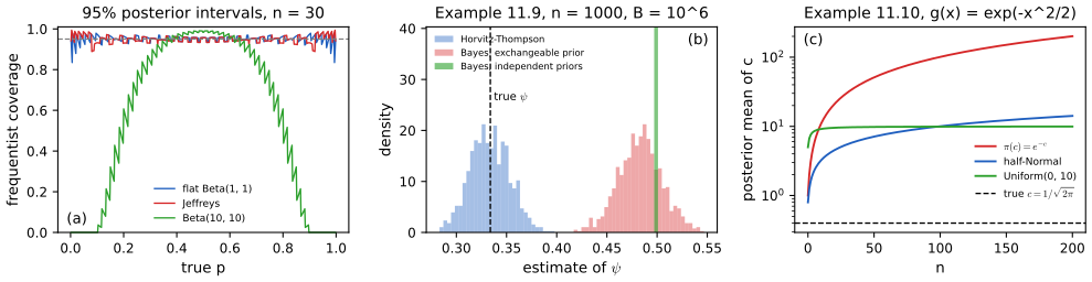
fig_11_s6. Download: PDF · SVGSee also (companion courses): posterior intervals for a proportion in Section 2.9.7 of Statistical Methods for Modern Biology; in this course, the coverage of the frequentist intervals for a proportion in the Chapter 6 coverage demo.
11.10 Bibliographic Remarks
pp. 189–190 The book points to the textbooks of Carlin and Louis (1996), Gelman, Carlin, Stern and Rubin (1995), Lee (1997), Robert (1994) and Schervish (1995); to Cox (1993), Diaconis and Freedman (1986), Freedman (1999), Barron, Schervish and Wasserman (1999), Ghosal, Ghosh and van der Vaart (2000), Shen and Wasserman (2001) and Zhao (2000) for the technicalities of nonparametric Bayesian inference (where Theorem 11.5 can fail); to Robins and Ritov (1997) for the full, nonparametric form of Example 11.9; to Berger and Delampady (1987) and Kass and Raftery (1995) for Bayesian testing; and to Kass and Wasserman (1996) for noninformative priors. Example 11.10 is credited in the book to a personal communication. For the Bernstein–von Mises theorem in full generality see van der Vaart (1998, Section 10.2); for the Dutch book argument, Ramsey (1926) and de Finetti (1937); for Jeffreys' rule, Jeffreys (1946).
11.11 Appendix
p. 190 The book's argument for Theorem 11.5, in outline. The effect of the prior fades as \(n\) grows, so \(f(\th\given\Xn)\propto L_n(\th)f(\th)\approx L_n(\th)\) and \(\log f(\th\given\Xn)\approx\ell(\th)\). Expand \(\ell\) to second order around the MLE, where \(\ell'(\hth)=0\): \(\ell(\th)\approx\ell(\hth)+\tfrac12(\th-\hth)^2\ell''(\hth)\). Exponentiating, \(f(\th\given\Xn)\propto\exp\{-\tfrac12(\th-\hth)^2/\sigma_n^2\}\) with \(\sigma_n^2=-1/\ell''(\hth)\), a Normal density with mean \(\hth\) and variance \(\sigma_n^2\). Finally, with \(\ell_i=\log f(X_i\given\th)\),
\[ \frac1{\sigma_n^2}=-\ell''(\hth)=\sum_i-\ell_i''(\hth)=n\Big(\frac1n\sum_i-\ell_i''(\hth)\Big)\approx n\,\E_\th\big(-\ell_i''(\hth)\big)=nI(\hth), \]so \(\sigma_n\approx\hse\).
Filling the gap 11.20: what the heuristic leaves out p. 190
Each "\(\approx\)" of the argument hides a step that Filling the gap 11.9 makes precise.
Details
(1) "The prior fades" really means that the prior is nearly constant on the shrinking region \(|\th-\hth|=O(1/\sqrt n)\) where the likelihood lives; this needs continuity and positivity of \(f\) at \(\th_0\), not just any prior (a prior that vanishes near \(\th_0\) can never be overcome). (2) The quadratic expansion is accurate only for \(|\th-\hth|=O(1/\sqrt n)\); away from \(\hth\) the posterior mass must be controlled separately, which is what the third-derivative bound (moderate distances) and the separation condition (large distances) do. A pointwise approximation of the density says nothing about the tails, while the conclusion \(\P(\th\in C_n\given\Xn)\to1-\alpha\) needs the whole distribution, hence the total variation (\(L^1\)) statement. (3) The average \(n^{-1}\sum_i-\ell_i''\) is evaluated at the random point \(\hth\), so the plain law of large numbers does not apply; the Lipschitz bound \(|\ell''(\hth)-\ell''(\th_0)|\le M|\hth-\th_0|\) closes this gap. (4) The last step writes \(\E_\th\) for the expectation that defines \(I\); the expectation is under the true \(\th_0\), and \(I(\hth)\approx I(\th_0)\) uses continuity of \(I\). ∎
Notes on the book
Five slips of Chapter 11 are in the author's errata lists; the other points below are mine, each with the evidence.
Page 177, equation (11.4): a missing \(\d\th\)
The numerator of the last expression for the posterior mean should be \(\int\th L_n(\th)f(\th)\,\d\th\). Listed in the author's errata.
Page 179, Example 11.2: \(d=\bth+1.96\tau\)
The upper end of the posterior interval is printed as \(\bth+1.96\), without \(\tau\) (Filling the gap 11.5). Listed in the author's errata.
Page 180, Example 11.3: the derivative of \(e^\psi/(1+e^\psi)\), and the final density
The derivative is \(e^\psi/(1+e^\psi)^2\), not \((1/(1+e^\psi))^2\) (listed in the author's errata). The error propagates to the final formula, which should read \(\big(\frac{e^\psi}{1+e^\psi}\big)^{s+1}\big(\frac1{1+e^\psi}\big)^{n-s+1}\) times the Beta constant: the printed version, with exponents \(s\) and \(n-s+2\), is the log-odds density of a different Beta distribution (Filling the gap 11.7); a Kolmogorov–Smirnov test on simulated draws rejects it decisively (Figure 11.S2(a)).
Page 182, improper priors: \(f(\th)\) should be \(f(\th\given\xn)\)
The display "\(f(\th)\propto L_n(\th)f(\th)\propto L_n(\th)\)" has the prior on the left where the posterior is meant; as printed it would say that the prior is proportional to the likelihood. Not in the errata lists.
Page 183, Example 11.6: "very close to a uniform density"
\(\Bet(1/2,1/2)\) is U-shaped and unbounded at 0 and 1, and its total variation distance from \(\Unif(0,1)\) is 0.21 (Filling the gap 11.13). The two priors give similar posteriors once both \(s\) and \(n-s\) are moderately large, which is presumably what is meant. A matter of wording, not in the errata lists.
Page 185, Example 11.8: \(\th\) should be unknown, not "known"
As in Example 6.14 (page 93), the example begins "Let \(\th\) be a fixed, known real number". The example's point, that after seeing \(Y=(15,17)\) "we are certain that \(\th=16\)", only makes sense if \(\th\) was unknown before the data; and the Bayesian analysis that follows puts a prior on \(\th\). Not in the errata lists (the same slip on page 93 is discussed in the Chapter 6 notes).
Page 186, Example 11.8: "is it" should be "it is"
The last sentence of the example should read "But it is not a probability statement about \(\th\)". Listed in the author's errata.
Page 186, Example 11.9: \((X_n,Y_n,R_n)\) should be \((X_n,R_n,Y_n)\)
The order of the last triple differs from the others. Listed in the author's errata.
Page 188, Example 11.9: "Horwitz" should be "Horvitz", and (11.11) can be sharpened
The estimator (11.10) is due to Horvitz and Thompson (1952). And the variance bound \(1/(n\delta^2)\) in (11.11) is correct but loose: the exact variance is \(n^{-1}(\E[\th_X/\xi_X]-\psi^2)\le1/(n\delta)\) (Filling the gap 11.17). Neither point is in the errata lists.
Page 189, Example 11.10: the posterior mean need not tend to infinity
The posterior mean \(\mu_{n+1}/\mu_n\) increases to the upper end of the prior's support: to infinity when the support is unbounded, but to 10 for a \(\Unif(0,10)\) prior, for instance; and for heavy-tailed priors (\(\mu_n=\infty\) for large \(n\)) there is no posterior at all (Filling the gap 11.18). The book's condition "\(\pi(c)>0\) for all \(c>0\)" does give an unbounded support, so the claim holds under it when the moments exist. A precision rather than an error; not in the errata lists.
11.12 Exercises
pp. 190–192 Each exercise is restated in my own words, followed by a worked solution. Computational answers come from the Python code (functions ex2 to ex8), with the seeds given there.
Exercise 11.1. Derive the Normal posterior (11.7).
Solution
This is Filling the gap 11.5: as a function of \(\th\), the likelihood is proportional to \(\exp\{-(\th-\overline x)^2/(2\se^2)\}\) because \(\sum_i(x_i-\th)^2=\sum_i(x_i-\overline x)^2+n(\th-\overline x)^2\); multiplying by the \(N(a,b^2)\) prior gives the exponential of a quadratic in \(\th\) with leading coefficient \(-\tfrac12(1/\se^2+1/b^2)\) and linear coefficient \(\overline x/\se^2+a/b^2\). Completing the square gives a Normal with precision \(1/\tau^2=1/\se^2+1/b^2\) and mean \(\tau^2(\overline x/\se^2+a/b^2)=w\overline x+(1-w)a\). It was confirmed numerically by normalising likelihood times prior on a fine grid.
Exercise 11.2. Let \(X_1,\dots,X_n\sim N(\mu,1)\). (a) Simulate \(n=100\) observations with \(\mu=5\). (b) With the flat prior \(f(\mu)=1\), find and plot the posterior density. (c) Draw 1000 values from the posterior, plot their histogram and compare with (b). (d) For \(\th=e^\mu\), find the posterior density analytically and by simulation. (e) Find a 95% posterior interval for \(\mu\). (f) Find a 95% interval for \(\th\).
Solution
(a) The simulated sample has \(\overline x=4.9916\) (sample standard deviation 0.956). (b) By Filling the gap 11.11(a) with \(\sigma=1\), \(\mu\given\xn\sim N(\overline x,1/n)=N(4.9916,0.1^2)\). (c) 1000 draws have mean 4.988 and standard deviation 0.101; their histogram follows the density (Figure 11.S7(a)). (d) \(\th=e^\mu\) is increasing with inverse \(\log\th\), so by the transformation formula
\[ h(\th\given\xn)=\frac1{\th}\,\frac{\sqrt n}{\sqrt{2\pi}}\exp\Big\{-\frac n2(\log\th-\overline x)^2\Big\},\qquad\th>0, \]a log-Normal density with median \(e^{\overline x}=147.2\) and mean \(e^{\overline x+1/(2n)}=147.9\); the exponentials of the 1000 draws follow it (Figure 11.S7(b)). (e) \(\overline x\pm1.96/\sqrt n=(4.796,5.188)\). (f) The book asks for a "confidence interval" here; both readings have the same answer. Since quantiles transform (Filling the gap 11.8(d)), the 95% posterior interval for \(\th\) is \((e^{4.796},e^{5.188})=(121.0,179.0)\), and because \((4.796,5.188)\) is also an exact 95% confidence interval for \(\mu\) and \(\exp\) is increasing, the same interval is an exact 95% confidence interval for \(\th\). The delta method gives instead \(e^{\overline x}(1\pm1.96/\sqrt n)=(118.3,176.0)\), symmetric and slightly shifted; the simulated quantiles give \((120.9,179.0)\).
Exercise 11.3. Let \(X_1,\dots,X_n\sim\Unif(0,\th)\) and \(f(\th)\propto1/\th\). Find the posterior density.
Solution
The likelihood is \(L_n(\th)=\th^{-n}\) if \(\th\ge x_{(n)}=\max_ix_i\) and 0 otherwise (each density \(1/\th\) on \((0,\th)\) must be positive at every \(x_i\)). So \(f(\th\given\xn)\propto\th^{-(n+1)}\) on \([x_{(n)},\infty)\), and since \(\int_{x_{(n)}}^\infty\th^{-(n+1)}\d\th=x_{(n)}^{-n}/n\),
\[ f(\th\given\xn)=\frac{n\,x_{(n)}^n}{\th^{n+1}},\qquad\th\ge x_{(n)}, \]a Pareto distribution. It is proper for every \(n\ge1\) although the prior is improper. Its mean is \(n\,x_{(n)}/(n-1)\) for \(n\ge2\), its median \(2^{1/n}x_{(n)}\), and the \(1-\alpha\) posterior interval with the lower end at \(x_{(n)}\) is \((x_{(n)},\alpha^{-1/n}x_{(n)})\). The prior \(1/\th\) is the Jeffreys-type prior for a scale parameter; the interval coincides with the exact confidence interval based on \(\P_\th(X_{(n)}/\th\le t)=t^n\).
Exercise 11.4. Of 50 patients on placebo 30 improve, and of 50 on a new treatment 40 improve. Let \(\tau=p_2-p_1\), with \(p_2\) the improvement probability under treatment and \(p_1\) under placebo. (a) Find the MLE of \(\tau\), its standard error and a 90% confidence interval by the delta method. (b) The same with the parametric bootstrap. (c) With the prior \(f(p_1,p_2)=1\), use simulation to find the posterior mean and a 90% posterior interval for \(\tau\). (d) For the log-odds ratio \(\psi=\log\frac{p_1}{1-p_1}-\log\frac{p_2}{1-p_2}\) find the MLE and a 90% delta-method interval. (e) Use simulation to find the posterior mean and a 90% posterior interval for \(\psi\).
Solution
(a) \(\widehat p_1=0.6\), \(\widehat p_2=0.8\), \(\widehat\tau=0.2\). The two estimates are independent, so
\[ \hse(\widehat\tau)=\sqrt{0.6\cdot0.4/50+0.8\cdot0.2/50}=\sqrt{0.008}=0.0894, \]and with \(z_{0.05}=1.645\) the interval is \(0.2\pm0.147=(0.053,0.347)\). (b) Drawing \(\widehat p_1^*=\Bin(50,0.6)/50\) and \(\widehat p_2^*=\Bin(50,0.8)/50\) 100 000 times, the standard deviation of \(\widehat p_2^*-\widehat p_1^*\) is 0.0892 and the Normal-based interval is \((0.053,0.347)\); the percentile interval is \((0.06,0.34)\). (c) The posterior is \(\Bet(31,21)\times\Bet(41,11)\) (Example 11.7). From 100 000 draws: posterior mean 0.192 (exactly \(41/52-31/52=0.1923\)) and 90% interval \((0.047,0.335)\), slightly shifted toward 0 because the flat prior pulls each proportion toward 1/2 (Figure 11.S2(c)). (d) \(\widehat\psi=\log(1.5)-\log(4)=-0.981\). The gradient of \(\psi\) is \((1/\{p_1(1-p_1)\},-1/\{p_2(1-p_2)\})\), so by the multivariate delta method (Theorem 5.15)
\[ \hse=\sqrt{1/(50\cdot0.24)+1/(50\cdot0.16)}=\sqrt{1/12+1/8}=0.456, \]and the 90% interval is \(-0.981\pm0.751=(-1.732,-0.230)\). (e) Transforming the same posterior draws: posterior mean \(-0.951\), 90% interval \((-1.696,-0.224)\). The two approaches agree closely, as Theorem 11.5 predicts with 50 observations per group.
Exercise 11.5. For the Bernoulli observations 0 1 0 1 0 0 0 0 0 0, plot the posterior for \(p\) under the priors \(\Bet(1/2,1/2)\), \(\Bet(1,1)\), \(\Bet(10,10)\) and \(\Bet(100,100)\).
Solution
Here \(s=2\), \(n=10\), and the posteriors are \(\Bet(2.5,8.5)\), \(\Bet(3,9)\), \(\Bet(12,18)\) and \(\Bet(102,108)\) (Filling the gap 11.4), with posterior means 0.227, 0.250, 0.400 and 0.486 and 95% intervals \((0.044,0.503)\), \((0.060,0.518)\), \((0.235,0.577)\) and \((0.418,0.553)\) (Figure 11.S7(c)). The first two are dominated by the data (the MLE is 0.2); \(\Bet(10,10)\) is worth 20 observations and pulls the posterior halfway to 1/2; \(\Bet(100,100)\) is worth 200 and the ten observations barely move it. With little data the prior matters.
Exercise 11.6. Let \(X_1,\dots,X_n\sim\Pois(\lambda)\). (a) With the prior \(\lambda\sim\Gam(\alpha,\beta)\), show that the posterior is Gamma and find its mean. (b) Find Jeffreys' prior and the posterior.
Solution
(a) With \(s=\sum_ix_i\), \(L_n(\lambda)=\prod_ie^{-\lambda}\lambda^{x_i}/x_i!\propto\lambda^se^{-n\lambda}\). With the prior density \(\propto\lambda^{\alpha-1}e^{-\beta\lambda}\) (shape \(\alpha\), rate \(\beta\)), the posterior is \(\propto\lambda^{\alpha+s-1}e^{-(\beta+n)\lambda}\), that is \(\lambda\given\xn\sim\Gam(\alpha+s,\beta+n)\), with mean
\[ \frac{\alpha+s}{\beta+n}=\frac n{\beta+n}\,\overline x+\frac\beta{\beta+n}\,\frac\alpha\beta, \]a weighted average of the MLE \(\overline x\) and the prior mean \(\alpha/\beta\); the prior is worth \(\beta\) observations. (If the Gamma is parametrised by a scale \(\beta\), replace \(\beta\) by \(1/\beta\).) (b) The score of one observation is \(x/\lambda-1\), so \(I(\lambda)=\V(X)/\lambda^2=1/\lambda\), and Jeffreys' prior is \(f(\lambda)\propto\lambda^{-1/2}\), improper (Filling the gap 11.13). The posterior is \(\propto\lambda^{s-1/2}e^{-n\lambda}\), the \(\Gam(s+\tfrac12,n)\) distribution, proper for every data set with \(n\ge1\) (even \(s=0\)), with mean \((s+\tfrac12)/n\). The Jeffreys-prior demo shows that the same posterior results whether the rule is applied to \(\lambda\), \(\log\lambda\), \(\sqrt\lambda\) or \(1/\lambda\).
Exercise 11.7. In Example 11.9, prove (11.11).
Solution
This is Filling the gap 11.17(c). The terms \(Z_i=R_iY_i/\xi_{X_i}\) are iid. Conditionally on \(X_i=j\), \(R_i\sim\Bern(\xi_j)\) and \(Y_i\sim\Bern(\th_j)\) independently, so \(\E(Z_i\given X_i=j)=\xi_j\th_j/\xi_j=\th_j\) and \(\E(Z_i)=B^{-1}\sum_j\th_j=\psi\). Hence \(\E\widehat\psi=\psi\). Next \(Z_i^2=R_iY_i/\xi_{X_i}^2\), so \(\E(Z_i^2\given X_i=j)=\th_j/\xi_j\le1/\delta\), and \(\V(Z_i)\le\E(Z_i^2)\le1/\delta\). Therefore \(\V(\widehat\psi)=\V(Z_1)/n\le1/(n\delta)\le1/(n\delta^2)\), the last step because \(0<\delta<1\). Both identities were confirmed exactly on a small population and by simulation with \(B=10^6\) cells.
Exercise 11.8. Let \(X\sim N(\mu,1)\) and test \(H_0:\mu=0\) against \(H_1:\mu\ne0\) with \(\P(H_0)=\P(H_1)=1/2\) and the prior \(\mu\sim N(0,b^2)\) under \(H_1\). Find \(\P(H_0\given X=x)\) and compare it with the p-value of the Wald test, numerically, for several \(x\) and \(b\). Repeat with a sample of size \(n\) and observe that \(\P(H_0\given\text{data})\) can be large while the p-value is small, especially for large \(n\) (the Jeffreys–Lindley paradox).
Solution
Under \(H_1\), \(X\) is marginally \(N(0,1+b^2)\), so
\[ \P(H_0\given x)=\frac{\phi(x)}{\phi(x)+(1+b^2)^{-1/2}\phi\big(x/\sqrt{1+b^2}\big)}, \]while the Wald p-value is \(2(1-\Phi(|x|))\). With \(n\) observations replace \(x\) by \(\overline x\), and the result is the formula of Filling the gap 11.15(d) in terms of \(z=\sqrt n\,\overline x\). Some values with \(n=1\):
\(x\) p-value \(b=0.5\) \(b=1\) \(b=3\) \(b=10\) bound 1.000 0.317 0.503 0.524 0.668 0.860 0.378 1.645 0.100 0.460 0.418 0.483 0.725 0.205 1.960 0.050 0.432 0.351 0.360 0.600 0.128 2.576 0.010 0.365 0.212 0.138 0.273 0.035 3.290 0.001 0.275 0.086 0.024 0.045 0.004 "bound" is the prior-free lower bound \(1/(1+e^{x^2/2})\). A p-value of 0.05 corresponds to a posterior probability of \(H_0\) between 0.35 and 0.60 for these priors, and never below 0.128 for any prior. With a sample of size \(n\) and the p-value fixed at 0.05 (\(z=1.96\)) and \(b=1\), \(\P(H_0\given\text{data})\) is 0.35, 0.60, 0.82, 0.94 and 0.993 for \(n=1\), \(10^2\), \(10^3\), \(10^4\) and \(10^6\) (Figure 11.S5(b)): the larger the sample, the more a "significant" result supports \(H_0\). Note that \(n\) and \(b\) enter only through \(nb^2\), so \(n=100\) with \(b=1\) gives the same answer as \(n=1\) with \(b=10\). The reason: with \(z\) fixed, \(\overline x=z/\sqrt n\to0\), a value that \(H_0\) predicts well and that \(H_1\), spreading its prediction over \(\mu\in\R\) with scale \(b\), predicts badly.
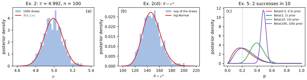
fig_11_s7. Download: PDF · SVGDemonstrations for this chapter
Each demonstration runs in the browser and links back to these notes. The ▶ Demo boxes above open them already set to the case under discussion.
| Demonstration | What you can see | Sections and results |
|---|---|---|
| Updating a proportion and the coverage of its posterior interval | The posterior interval updated one toss at a time; the interval for every possible outcome with the binomial probabilities; the exact frequentist coverage against \(p\), its minimum, and its average over the prior. Presets: 1 Example 11.1; 2 Jeffreys' prior; 3 a confident prior far from the truth; 4 the same prior when it is right; 5 the prior washes out. | Example 11.1, 11.9; Filling the gaps 11.6, 11.19 |
| The posterior becomes Normal | The exact posterior against \(N(\hth,\hse^2)\) for coin tosses or the nerve data, their total variation distance against \(n\), and the posterior probability of the Wald interval, in the natural or the log scale, under three priors. Presets: 1 a fair coin; 2 a rare event; 3 the log-odds scale; 4 the nerve data; 5 a confident, wrong prior. | Theorem 11.5, 11.11; Filling the gaps 11.9, 11.10 |
| Flat priors, Jeffreys' prior and reparametrisation | The flat or Jeffreys rule applied to \(p\) (or \(\lambda\)) and to a transformed parameter, carried between the scales with the Jacobian; the resulting posteriors; the Fisher information computed from the score in each scale. Presets: 1 flat on \(p\) or on the log-odds; 2 Jeffreys; 3 the variance-stabilising scale; 4 an improper posterior; 5 Poisson counts. | 11.6, Example 11.6, Exercise 11.6; Filling the gaps 11.11–11.13 |
Related demonstrations in the companion courses: the conjugate-prior demo and the Bayesian linear regression demo of Bayesian and Probabilistic Machine Learning, the beta-binomial demo of Statistical Methods for Modern Biology, and, in this course, the Chapter 1 base-rate demo for Bayes' theorem with events. The Python code that produces every figure of this page is code/ch11_bayesian_inference.py (see the code index).
References
- Wasserman, L. (2004). All of Statistics: A Concise Course in Statistical Inference. Springer, New York. Chapter 11, pp. 175–192. www.stat.cmu.edu/~larry/all-of-statistics.
- Barron, A., Schervish, M. J. and Wasserman, L. (1999). The consistency of posterior distributions in nonparametric problems. The Annals of Statistics, 27(2), 536–561.
- Berger, J. O. and Delampady, M. (1987). Testing precise hypotheses. Statistical Science, 2(3), 317–335.
- Berger, J. O. and Sellke, T. (1987). Testing a point null hypothesis: the irreconcilability of P values and evidence. Journal of the American Statistical Association, 82(397), 112–122.
- Berger, J. O. and Wolpert, R. L. (1984). The Likelihood Principle. Institute of Mathematical Statistics, Hayward, California.
- Brown, L. D., Cai, T. T. and DasGupta, A. (2001). Interval estimation for a binomial proportion. Statistical Science, 16(2), 101–133.
- Carlin, B. P. and Louis, T. A. (1996). Bayes and Empirical Bayes Methods for Data Analysis. Chapman and Hall, London.
- Cox, D. D. (1993). An analysis of Bayesian inference for nonparametric regression. The Annals of Statistics, 21(2), 903–923.
- Cox, D. R. and Lewis, P. A. W. (1966). The Statistical Analysis of Series of Events. Methuen, London. (Source of the nerve data.)
- de Finetti, B. (1937). La prévision: ses lois logiques, ses sources subjectives. Annales de l'Institut Henri Poincaré, 7(1), 1–68.
- Diaconis, P. and Freedman, D. (1986). On the consistency of Bayes estimates. The Annals of Statistics, 14(1), 1–26.
- Freedman, D. (1999). On the Bernstein–von Mises theorem with infinite-dimensional parameters. The Annals of Statistics, 27(4), 1119–1140.
- Gelman, A., Carlin, J. B., Stern, H. S. and Rubin, D. B. (1995). Bayesian Data Analysis. Chapman and Hall, London.
- Ghosal, S., Ghosh, J. K. and van der Vaart, A. W. (2000). Convergence rates of posterior distributions. The Annals of Statistics, 28(2), 500–531.
- Horvitz, D. G. and Thompson, D. J. (1952). A generalization of sampling without replacement from a finite universe. Journal of the American Statistical Association, 47(260), 663–685.
- Jeffreys, H. (1946). An invariant form for the prior probability in estimation problems. Proceedings of the Royal Society of London, Series A, 186(1007), 453–461.
- Kass, R. E. and Raftery, A. E. (1995). Bayes factors. Journal of the American Statistical Association, 90(430), 773–795.
- Kass, R. E. and Wasserman, L. (1996). The selection of prior distributions by formal rules. Journal of the American Statistical Association, 91(435), 1343–1370.
- Lee, P. M. (1997). Bayesian Statistics: An Introduction, 2nd edition. Arnold, London.
- Lindley, D. V. (1957). A statistical paradox. Biometrika, 44(1/2), 187–192.
- Ramsey, F. P. (1926). Truth and probability. Published in The Foundations of Mathematics and Other Logical Essays (1931), Routledge and Kegan Paul, London.
- Robert, C. P. (1994). The Bayesian Choice. Springer, New York.
- Robins, J. M. and Ritov, Y. (1997). Toward a curse of dimensionality appropriate (CODA) asymptotic theory for semi-parametric models. Statistics in Medicine, 16(3), 285–319.
- Schervish, M. J. (1995). Theory of Statistics. Springer, New York.
- Shen, X. and Wasserman, L. (2001). Rates of convergence of posterior distributions. The Annals of Statistics, 29(3), 687–714.
- van der Vaart, A. W. (1998). Asymptotic Statistics. Cambridge University Press, Cambridge.
- Zhao, L. H. (2000). Bayesian aspects of some nonparametric problems. The Annals of Statistics, 28(2), 532–552.
The numerical statements in the text (the conjugate posteriors and their summaries, the loss-minimising property of the posterior mean and median, the log-odds density and its mean, the posterior of \(p_2-p_1\), the total variation distances and posterior probabilities of the Wald interval for the nerve data and the coin tosses, the Fisher information in every parametrisation used and the invariance of Jeffreys' prior, the distance between \(\Bet(1/2,1/2)\) and the uniform, the multiparameter Normal information, the posterior probabilities of a point null, their minima and the Lindley limit, the exact and prior-averaged coverage of Beta posterior intervals, the Robins–Ritov simulation and the Horvitz–Thompson variance, the posterior means of the normalising constant, and the solutions of the exercises) were confirmed numerically.