Probability Redux: Stochastic Processes
Almost everything earlier in the book is about independent observations. This chapter lets the past matter, in the two simplest ways that still have a rich theory. In a Markov chain the next state depends on the present one only; the questions are whether the chain settles into an equilibrium, how fast, and how to estimate its transition probabilities. In a Poisson process events arrive "completely at random" in time; the questions are what the gaps between them look like and how to test that the rate is constant. The book states the main theorems of Markov chain theory (the recurrence criterion, the classification of states, the convergence to the stationary distribution, the ergodic theorem, the asymptotics of the maximum likelihood estimator) without proof, and proves the Poisson results only informally. These notes supply complete proofs, built on two ideas: the first-passage decomposition, which turns questions about returns into generating functions, and coupling, which proves convergence by making two copies of the chain meet.
Ch. 1 Probability Ch. 2 Random variables Ch. 3 Expectation Ch. 4 Inequalities Ch. 5 Convergence Ch. 6 Models and inference Ch. 7 Estimating the CDF Ch. 8 Bootstrap Ch. 9 Parametric inference Ch. 10 Hypothesis testing Ch. 11 Bayesian inference Ch. 12 Decision theory Ch. 13 Regression Ch. 14 Multivariate models Ch. 15 Independence Ch. 16 Causal inference Ch. 17 Directed graphs Ch. 18 Undirected graphs Ch. 19 Log-linear models Ch. 20 Curve estimation Ch. 21 Orthogonal functions Ch. 22 Classification Ch. 23 Stochastic processes Ch. 24 Simulation
How to read these notes
They follow the book. Sections carry the book's numbers (23.1 to 23.5); Section 23.2 is split along the book's own run-in headings (transition probabilities, states, convergence, examples, inference). Numbered items keep the book's numbers (Definition 23.5, Theorem 23.9, ..., Example 23.36) and numbered equations keep theirs, \((23.1)\) to \((23.17)\). Results the book uses without a number, and the new results needed to fill its gaps, are lettered (Definition 23.A, Theorem 23.D, ...).
Filling the gaps. Wherever the book says "it can be shown", quotes a result without proof, or leaves an argument informal, an orange Filling the gap box gives the full argument. Proofs and derivations start hidden: open one with its bar, or use the button below.
Figures and demonstrations. The three figures of the chapter are reproduced: Figures 23.1 and 23.2 by new simulations (as in the book), and Figure 23.3 with a simulated stand-in, because the book does not distribute its web server data. Five supplementary figures (23.S1 to 23.S5) illustrate gaps filled in the notes and two exercises. All are produced by the Python code. The ▶ Demo boxes open an interactive demonstration already set to the case being discussed.
Main reference
L. Wasserman, All of Statistics: A Concise Course in Statistical Inference, Springer (2004), Chapter 23, pages 381–401 (book website: www.stat.cmu.edu/~larry/all-of-statistics). Section, equation, example and exercise numbers below refer to this book. Further reading is listed in the references.
The explanations, derivations, figures and code are my own; equations are cited by their numbers in the book.
Companion courses
Markov chains and Poisson counts appear in four companion courses on this site. The overlapping material is:
- Bayesian and Probabilistic Machine Learning, Section 11.2.1 (Markov chains for sampling): homogeneity, invariance and detailed balance (Definition 11.1, Result 11.16), geometric convergence of a finite chain with a positive power \(\Pm^m\) by a Doeblin argument (Result 11.17), and Metropolis-Hastings (Result 11.19); its MCMC demo. Also Section 13.1 (Markov models of sequences) and Section 13.2 (hidden Markov models, with the stationary distribution of the hidden chain in Result 13.5), and its HMM demo.
- Statistical Learning: Theory and Methods, Section 14.10: PageRank is the stationary distribution of a random surfer's chain (see also its note on the two normalisations), with the PageRank demo.
- Statistical Methods for Modern Biology, Section 2.8: Markov chains for DNA (Definition 2.5), transition probabilities estimated by counting, and the CpG island demo; Hardy-Weinberg proportions in Section 2.7.2.
Those courses use Markov chains as tools (to sample, to model sequences, to rank pages) and mostly for finite chains with a positive power of \(\Pm\). Here the general countable theory is developed: recurrence and transience (Filling the gap 23.5), random walks and Pólya's theorem (23.7), stationary distributions and mean return times (Theorem 23.D), a coupling proof of convergence that needs no positive power (23.11), the ergodic theorem (23.11) and the asymptotics of the transition-probability MLE (23.17). Where a companion course already proves a finite-chain result in full, the statement here is followed by a shorter argument and a link.
The chapter at a glance
- 23.1 A stochastic process is a family of random variables indexed by time; its law is fixed by its finite-dimensional distributions, and any joint density factorises into conditionals given the past, \((23.1)\).
- 23.2 A Markov chain forgets everything but the present. Its \(n\)-step transition matrix is \(\Pm^n\) (Chapman-Kolmogorov) and the law of \(X_n\) is \(\mu_0\Pm^n\). States split into communicating classes; a state is recurrent exactly when the expected number of returns is infinite (Theorem 23.15). An irreducible, aperiodic, positive recurrent chain converges to its unique stationary distribution, and time averages converge to stationary means (Theorem 23.25). The MLE of \(p_{ij}\) is \(n_{ij}/n_i\), consistent and asymptotically Normal (Theorem 23.31).
- 23.3 A Poisson process has independent increments and rate \(\lambda(t)\); its counts are Poisson with mean \(\int\lambda\) (Theorem 23.33). For a constant rate the gaps are iid exponential (Theorem 23.35) and, given their number, the event times are uniform order statistics (Theorem 23.F), which is what the test of Example 23.36 uses.
Notation. \(\Xc\) is the state space (finite or countable for chains), \(\P_i\) and \(\E_i\) are probability and expectation for the chain started at \(X_0=i\), \(\P_\mu\) for \(X_0\sim\mu\). \(p_{ij}(n)\) is an \(n\)-step transition probability, with \(p_{ij}(0)=\ind\{i=j\}\). Distributions on \(\Xc\) are row vectors. For a Poisson process, \(X(t)\) counts events in \([0,t]\) and \(W_n\) is the time of the \(n\)th event.
Prerequisites. Conditional probability and the law of total probability (Chapter 1), the Poisson, exponential and gamma laws (Result 2.6, Result 2.8), order statistics (Result 2.21), generating functions (Section 3.6), the strong law of large numbers (Theorem 5.18) and the central limit theorem (Theorem 5.8), the multinomial MLE (Theorem 14.5) and Pearson's \(\chi^2\) test (Theorem 10.17). See the course home.
23.1 Introduction
p. 381 Daily temperatures, the price of a share, the letters along a DNA molecule: in each case consecutive observations are dependent, and the order in which they come matters. The object that models such data is a whole collection of random variables indexed by time.
Definition 23.A (stochastic process, state space, index set, sample path) p. 381
A stochastic process \(\{X_t:t\in T\}\) is a collection of random variables on one probability space, all taking values in a set \(\Xc\), the state space. The index set \(T\) is thought of as time: discrete, \(T=\{0,1,2,\dots\}\), or continuous, \(T=[0,\infty)\). We also write \(X(t)\) for \(X_t\). For each outcome \(\omega\), the function \(t\mapsto X_t(\omega)\) is a sample path. The finite-dimensional distributions of the process are the joint laws of \((X_{t_1},\dots,X_{t_k})\) for all finite sets of times \(t_1<\dots<t_k\).
Examples 23.1 to 23.4 pp. 381–382
23.1 (iid observations). An iid sequence \(X_1,X_2,\dots\) is a process with \(T=\{1,2,\dots\}\); every finite-dimensional distribution is a product.
23.2 (the weather). \(\Xc=\{\text{sunny},\text{cloudy}\}\) and \(T=\{0,1,2,\dots\}\): a discrete state space and a discrete index set.
23.3 (stock prices). A price recorded continuously: \(T=[0,\infty)\), and the price, though discrete in cents, can be treated as continuous. Figure 23.1 shows a simulated price.
23.4 (the empirical cdf). For \(X_1,\dots,X_n\sim F\) on \([0,1]\), \(\{\widehat F_n(t):t\in[0,1]\}\) is a process with continuous index set; its finite-dimensional distributions are multinomial (Filling the gap 7.2). The Glivenko-Cantelli theorem and the DKW inequality (Theorems 7.4 and 7.5) are statements about the whole sample path at once, \(\sup_t|\widehat F_n(t)-F(t)|\), which is why the process point of view is useful there.
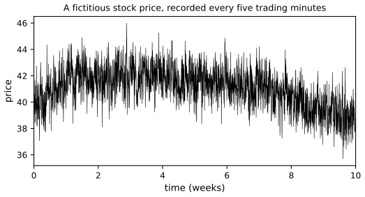
fig_23_1. Download: PDF · SVGp. 382 Whatever the dependence, a joint density (or mass function) of \(X_1,\dots,X_n\) factorises into one-step conditionals:
\[ f(x_1,\dots,x_n)=f(x_1)f(x_2\given x_1)\cdots f(x_n\given x_1,\dots,x_{n-1})=\prod_{i=1}^nf(x_i\given\text{past}_i), \tag{23.1} \]with \(\text{past}_i=(X_1,\dots,X_{i-1})\). The models of this chapter are defined by restricting how \(f(x_i\given\text{past}_i)\) may depend on the past.
Filling the gap 23.1: why (23.1) holds, and when finite-dimensional distributions define a process pp. 381–382
The chain rule. \((23.1)\) holds at every \((x_1,\dots,x_n)\) with \(f(x_1,\dots,x_{n-1})>0\); where a marginal vanishes, both sides are 0 under the usual convention that a conditional density is set arbitrarily (say to 0) where the conditioning density is 0.
Building a process. A process with index set \(\{0,1,2,\dots\}\) involves infinitely many random variables, and one must check that they can live on one probability space. Kolmogorov's extension theorem says that any family of finite-dimensional distributions that is consistent (the law of \((X_{t_1},\dots,X_{t_k})\) is the margin of the law of any larger set of times) is the family of some process. For the processes of this chapter there is a direct construction from a single sequence \(U_1,U_2,\dots\) of iid Uniform\((0,1)\) variables (Algorithm 23.A for Markov chains, Theorem 23.E for Poisson processes), and such a sequence exists on \([0,1]\) with Lebesgue measure: split the binary digits of one uniform into infinitely many disjoint infinite subsequences.
Proof of the chain rule
By induction on \(n\). For \(n=1\) there is nothing to prove. If it holds for \(n-1\), the definition of the conditional density of \(X_n\) given \((X_1,\dots,X_{n-1})\) (Definition 2.9) gives \(f(x_1,\dots,x_n)\)
23.2 Markov Chains
p. 383 In this section the state space is discrete, \(\Xc=\{1,\dots,N\}\) or \(\Xc=\{1,2,\dots\}\), and time is \(\{0,1,2,\dots\}\), written \(n\).
Definition 23.5 (Markov chain) p. 383
\(\{X_n:n\ge0\}\) is a Markov chain if, for all \(n\ge1\) and all \(x\in\Xc\),
\[ \P(X_n=x\given X_0,\dots,X_{n-1})=\P(X_n=x\given X_{n-1}). \tag{23.2} \]Equivalently, \((23.1)\) simplifies to \(f(x_0,\dots,x_n)\)
The book sets three questions: when does a chain settle into an equilibrium, how are its parameters estimated, and how can one build a chain with a prescribed equilibrium (the subject of the book's Chapter 24, Markov chain Monte Carlo)? The first two are answered here. Everything rests on using \((23.2)\) in stronger forms than it is stated in.
Theorem 23.B (equivalent forms of the Markov property)
For a process with discrete states, the following are equivalent.
- \((23.2)\) holds (for all conditioning values of positive probability).
- For every \(n\) and every path, \(\P(X_0=x_0,\dots,X_n=x_n)\)
\({}=\mu_0(x_0)\prod_{k=1}^np_{x_{k-1}x_k}^{(k)}\), where \(\mu_0\) is the law of \(X_0\) and \(p^{(k)}_{ij}=\P(X_k=j\given X_{k-1}=i)\). - (past and future are independent given the present) For all \(n,m\ge1\), states \(i,j_1,\dots,j_m\), and every event \(A\) determined by \((X_0,\dots,X_{n-1})\) with \(\P(A,X_n=i)>0\), \[ \P(X_{n+1}=j_1,\dots,X_{n+m}=j_m\given A,\,X_n=i)=\P(X_{n+1}=j_1,\dots,X_{n+m}=j_m\given X_n=i). \]
For a homogeneous chain (below) the right side of (3) is \(p_{ij_1}p_{j_1j_2}\cdots p_{j_{m-1}j_m}\), whatever \(n\).
Filling the gap 23.2: proof of Theorem 23.B, and why it is needed pp. 383–386
The proof of the Chapman-Kolmogorov equations (Theorem 23.9) replaces \(\P(X_{m+n}=j\given X_m=k,X_0=i)\) by \(\P(X_{m+n}=j\given X_m=k)\). That is not \((23.2)\): the conditioning is on part of the past (\(X_0\) only), and the target is \(n\) steps ahead. Part (3) with \(A=\{X_0=i\}\) is exactly what is used.
Proof
(1) \(\Rightarrow\) (2): the chain rule \((23.1)\) for mass functions, with each factor \(\P(X_k=x_k\given X_0=x_0,\dots,X_{k-1}=x_{k-1})\) replaced by \(p^{(k)}_{x_{k-1}x_k}\) using (1). (If some prefix of the path has probability 0, both sides are 0.)
(2) \(\Rightarrow\) (3): \(A\) is a union of paths \((x_0,\dots,x_{n-1})\) over some set \(S\). By (2),
\[ \P(A,X_n=i,X_{n+1}=j_1,\dots,X_{n+m}=j_m)=\sum_{(x_0,\dots,x_{n-1})\in S}\mu_0(x_0)\Big[\prod_{k=1}^{n}p^{(k)}_{x_{k-1}x_k}\Big]_{x_n=i}\cdot\prod_{l=1}^mp^{(n+l)}_{j_{l-1}j_l}, \]with \(j_0=i\). The last product does not depend on the path, so this equals \(\P(A,X_n=i)\prod_lp^{(n+l)}_{j_{l-1}j_l}\). Dividing by \(\P(A,X_n=i)\) shows that the conditional probability equals \(\prod_lp^{(n+l)}_{j_{l-1}j_l}\) for every such \(A\); taking \(A\) to be the sure event shows that this is also \(\P(\cdot\given X_n=i)\).
(3) \(\Rightarrow\) (1): take \(m=1\) and \(A=\{X_0=x_0,\dots,X_{n-2}=x_{n-2}\}\) (shifting \(n\) by one). ∎
Algorithm 23.A (simulating a Markov chain) p. 386
Given \(\mu_0\) and \(\Pm\), and iid \(U_0,U_1,U_2,\dots\sim\) Uniform\((0,1)\), with states listed as \(1,2,\dots\):
- \(X_0=\) the smallest \(j\) with \(U_0<\mu_0(1)+\dots+\mu_0(j)\).
- For \(n=0,1,2,\dots\): \(X_{n+1}=\phi(X_n,U_{n+1})\), where \(\phi(i,u)=\) the smallest \(j\) with \(u<p_{i1}+\dots+p_{ij}\).
This is the book's step-by-step recipe written as a formula. It produces a Markov chain with initial law \(\mu_0\) and transition matrix \(\Pm\): \(X_0,\dots,X_n\) are functions of \(U_0,\dots,U_n\), so \(U_{n+1}\) is independent of them, and \(\P(X_{n+1}=j\given X_0,\dots,X_n=i)\)
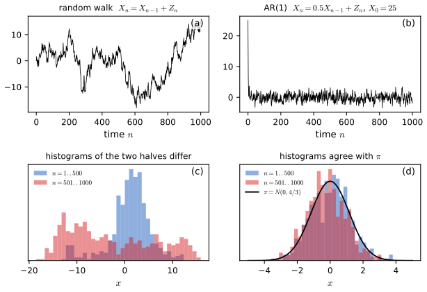
fig_23_2. Download: PDF · SVGTransition probabilities
p. 384 A chain is homogeneous if \(\P(X_{n+1}=j\given X_n=i)\) does not depend on \(n\). From here on all chains are homogeneous.
Definition 23.6 (transition probabilities, transition matrix) p. 384
\[ p_{ij}\equiv\P(X_{n+1}=j\given X_n=i) \tag{23.3} \]are the transition probabilities, and the matrix \(\Pm=(p_{ij})\) is the transition matrix. It is stochastic: \(p_{ij}\ge0\) and every row sums to one, \(\sum_jp_{ij}=1\) (the book writes \(\sum_i\), a slip: see the notes on the book). Row \(i\) is the law of the next state from \(i\).
Examples 23.7 and 23.8 pp. 384–385
23.7 (random walk with absorbing barriers). On \(\{1,\dots,N\}\), step right with probability \(p\), left with \(q=1-p\), and stay for ever at 1 or \(N\) once there: \(p_{11}=p_{NN}=1\) and \(p_{i,i+1}=p\), \(p_{i,i-1}=q\) for \(1<i<N\).
23.8 (the weather). With states (sunny, cloudy),
\[ \Pm=\begin{pmatrix}0.4&0.6\\0.8&0.2\end{pmatrix}: \]after a sunny day, the next is cloudy with probability 0.6. Its stationary distribution is \(\pi=(4/7,3/7)\) (Exercise 23.3 with \(a=0.6\), \(b=0.8\)).
p. 385 The \(n\)-step transition probabilities are
\[ p_{ij}(n)=\P(X_{m+n}=j\given X_m=i), \tag{23.4} \]which by homogeneity (and Theorem 23.B(3)) do not depend on \(m\); \(\Pm_n\) is the matrix of them.
Theorem 23.9 (the Chapman-Kolmogorov equations) p. 385
\[ p_{ij}(m+n)=\sum_kp_{ik}(m)\,p_{kj}(n). \tag{23.5} \]In matrix form \(\Pm_{m+n}=\Pm_m\Pm_n\) \((23.6)\), and since \(\Pm_1=\Pm\), induction gives \(\Pm_n=\Pm^n\), the \(n\)th matrix power \((23.7)\).
Proof
By the law of total probability over the state at time \(m\), then the multiplication rule, then Theorem 23.B(3) with \(A=\{X_0=i\}\) (which removes \(X_0\) from the conditioning):
\[ p_{ij}(m+n)=\sum_k\P(X_m=k\given X_0=i)\,\P(X_{m+n}=j\given X_m=k,X_0=i)=\sum_kp_{ik}(m)\,p_{kj}(n), \]the sum running over \(k\) with \(p_{ik}(m)>0\) (the other terms vanish). All terms are nonnegative, so the countable sum is unproblematic. ∎
Lemma 23.10 (the marginal distributions) p. 387
Let \(\mu_n=(\mu_n(1),\mu_n(2),\dots)\) with \(\mu_n(i)=\P(X_n=i)\) \((23.8)\); \(\mu_0\) is the initial distribution. Then \(\mu_n=\mu_0\Pm^n\).
Proof
\(\mu_n(j)\)
Filling the gap 23.3: powers of a stochastic matrix, and the two-state chain pp. 385–387
(a) Products of stochastic matrices are stochastic, so \(\Pm^n\) is a transition matrix and \(\mu_0\Pm^n\) a distribution. (b) For two states with \(p_{12}=a\), \(p_{21}=b\), \(0<a+b<2\),
\[ \Pm^n=\frac1{a+b}\begin{pmatrix}b&a\\b&a\end{pmatrix}+\frac{(1-a-b)^n}{a+b}\begin{pmatrix}a&-a\\-b&b\end{pmatrix}. \]So \(\mu_n\) approaches \(\pi=(b,a)/(a+b)\) at the geometric rate \(|1-a-b|\): for the weather chain the rate is \(|1-0.6-0.8|=0.4\), and the distance to \(\pi\) after 10 days is \(4.5\times10^{-5}\) from a sunny start (Figure 23.S1(a)). This is Exercise 23.3.
Proof
(a) If \(\Pm,\mathbf Q\) are stochastic, \((\Pm\mathbf Q)_{ij}\)
Summary of terminology p. 387: transition matrix \(\Pm(i,j)=p_{ij}\); \(n\)-step matrix \(\Pm_n(i,j)=p_{ij}(n)=(\Pm^n)_{ij}\); marginal \(\mu_n(i)=\P(X_n=i)\); \(\mu_n=\mu_0\Pm^n\).
States
p. 387 States are classified by which other states they can reach, and by whether the chain comes back to them.
Definition 23.11 (accessible, communicate) p. 387
\(i\) reaches \(j\) (\(j\) is accessible from \(i\)), written \(i\to j\), if \(p_{ij}(n)>0\) for some \(n\ge0\), with the convention \(p_{ii}(0)=1\). If \(i\to j\) and \(j\to i\), then \(i\) and \(j\) communicate, \(i\lra j\).
Theorem 23.12 (communication is an equivalence relation) p. 387
(1) \(i\lra i\); (2) \(i\lra j\Rightarrow j\lra i\); (3) \(i\lra j\) and \(j\lra k\Rightarrow i\lra k\); (4) hence \(\Xc\) is a disjoint union of classes \(\Xc_1,\Xc_2,\dots\), two states communicating exactly when they are in the same class.
Filling the gap 23.4: proof of Theorem 23.12, the \(n=0\) convention, and closed classes pp. 387–388
The book allows "some \(n\)" without saying whether \(n=0\) counts. It must: in Example 23.7 with \(N=3\), state 2 moves to an absorbing end point at the first step, so \(p_{22}(n)=0\) for every \(n\ge1\), and without \(n=0\) part (1) fails for state 2.
The chain is irreducible if there is a single class. A set \(C\) is closed if \(p_{ij}=0\) for \(i\in C\), \(j\notin C\) (then \(p_{ij}(n)=0\) for all \(n\): the chain never leaves \(C\)); a closed set \(\{i\}\) is an absorbing state, \(p_{ii}=1\). In Example 23.13 (\(\Xc=\{1,2,3,4\}\), rows \((\tfrac13,\tfrac23,0,0)\), \((\tfrac23,\tfrac13,0,0)\), \((\tfrac14,\tfrac14,\tfrac14,\tfrac14)\), \((0,0,0,1)\)) the classes are \(\{1,2\}\) (closed), \(\{3\}\) (not closed) and \(\{4\}\) (absorbing); the code finds them by computing which states reach which (a transitive closure) and grouping mutually reachable ones.
Proof
(1) \(p_{ii}(0)=1>0\). (2) The definition is symmetric. (3) If \(p_{ij}(m)>0\) and \(p_{jk}(n)>0\), Chapman-Kolmogorov gives \(p_{ik}(m+n)\ge p_{ij}(m)p_{jk}(n)>0\); the same holds in the reverse direction. (4) Any equivalence relation partitions its set into equivalence classes: the class of \(i\) is \(\{j:j\lra i\}\); two classes that share a state coincide by (2) and (3), and every state lies in its own class by (1). For "closed implies never leaves": if \(i\in C\), \(p_{ij}(n+1)=\sum_kp_{ik}(n)p_{kj}\), and by induction \(p_{ik}(n)=0\) for \(k\notin C\), while \(p_{kj}=0\) for \(k\in C\), \(j\notin C\). ∎
Definition 23.14 (recurrent, transient) p. 388
State \(i\) is recurrent (persistent) if \(\P(X_n=i\text{ for some }n\ge1\given X_0=i)\)
Theorem 23.15 (the recurrence criterion) p. 388
\[ i\text{ is recurrent}\iff\sum_{n}p_{ii}(n)=\infty, \tag{23.9} \] \[ i\text{ is transient}\iff\sum_np_{ii}(n)<\infty. \tag{23.10} \]More precisely, \(\sum_{n\ge0}p_{ii}(n)=1/(1-f_{ii})\), the expected number of visits to \(i\) (counting time 0) of the chain started at \(i\).
The book's proof writes the expected number of visits as \(\sum_np_{ii}(n)\) and then argues that a chain that returns with probability one returns again and again. The repeated-return argument needs the chain to "start afresh" at a random time, the return time; the next box proves the criterion in two ways, first without random times at all.
First-passage probabilities p. 390, (23.12)–(23.13)
For \(n\ge1\) let \(f_{ij}(n)\)
Filling the gap 23.5: proof of Theorem 23.15 (first passages and the renewal equation) pp. 388–389
The first-passage decomposition. For \(n\ge1\) and all \(i,j\),
\[ p_{ij}(n)=\sum_{k=1}^nf_{ij}(k)\,p_{jj}(n-k). \]Generating functions. For \(0\le s<1\) put \(P_{ij}(s)=\sum_{n\ge0}p_{ij}(n)s^n\) and \(F_{ij}(s)=\sum_{n\ge1}f_{ij}(n)s^n\). The decomposition is a convolution, so
\[ P_{ii}(s)=1+F_{ii}(s)P_{ii}(s),\qquad P_{ij}(s)=F_{ij}(s)P_{jj}(s)\ (i\ne j). \]Hence \(P_{ii}(s)=1/(1-F_{ii}(s))\), and letting \(s\uparrow1\) (monotone convergence on both sides) gives \(\sum_np_{ii}(n)=1/(1-f_{ii})\), which is infinite exactly when \(f_{ii}=1\). This proves \((23.9)\) and \((23.10)\). The second identity gives, for \(i\ne j\),
\[ \sum_{n\ge0}p_{ij}(n)=f_{ij}\sum_{n\ge0}p_{jj}(n), \]so if \(j\) is transient then \(\sum_np_{ij}(n)<\infty\) and \(p_{ij}(n)\to0\) from every start. In Example 23.28 below, state 3 returns with probability \(f_{33}=1/3\) and is visited \(1/(1-1/3)=3/2\) times on average, numbers the code obtains from the first-passage probabilities and confirms by simulation.
The book's argument, made precise. Let \(V\) be the number of visits to \(i\). By the strong Markov property (Theorem 23.C) applied at the \(k\)th return time, \(\P_i(V\ge k+1)=f_{ii}^{\,k}\): \(V\) is geometric with mean \(1/(1-f_{ii})\) when \(f_{ii}<1\), and \(V=\infty\) almost surely when \(f_{ii}=1\). Since \(V=\sum_n\ind\{X_n=i\}\), \(\E_iV=\sum_np_{ii}(n)\) (monotone convergence), the same identity.
Proofs
Decomposition. The events \(B_k\)
Generating functions. All series have nonnegative terms bounded by \(s^n\), so they converge for \(s<1\) and may be multiplied termwise: \(\sum_{n\ge1}s^n\sum_{k=1}^nf_{ij}(k)p_{jj}(n-k)\)
The geometric number of visits. Let \(\tau_k\) be the time of the \(k\)th return (\(\tau_k=\infty\) if there are fewer). \(\tau_k\) is a stopping time, and on \(\{\tau_k<\infty\}\), \(X_{\tau_k}=i\). By Theorem 23.C the chain after \(\tau_k\) is a copy started at \(i\), independent of the past, so \(\P_i(\tau_{k+1}<\infty\given\tau_k<\infty)\)
Theorem 23.C (the strong Markov property)
A random time \(\tau\in\{0,1,\dots,\infty\}\) is a stopping time if each event \(\{\tau=n\}\) is determined by \(X_0,\dots,X_n\) (the first visit to a state is one; the last visit is not). Then, given \(\tau<\infty\) and \(X_\tau=i\), the process \((X_{\tau+m})_{m\ge0}\) is a Markov chain with transition matrix \(\Pm\) started at \(i\), and it is independent of \((X_0,\dots,X_\tau)\).
Proof
Let \(A\) be an event determined by \((\tau,X_0,\dots,X_\tau)\) on \(\{\tau<\infty\}\). Then \(A\cap\{\tau=n\}\) is determined by \(X_0,\dots,X_n\), and Theorem 23.B(3) gives
\[ \P(A,\tau=n,X_n=i,X_{n+1}=j_1,\dots,X_{n+m}=j_m)=\P(A,\tau=n,X_n=i)\,p_{ij_1}\cdots p_{j_{m-1}j_m}. \]Summing over \(n\) gives \(\P(A,\tau<\infty,X_\tau=i,X_{\tau+1}=j_1,\dots)\)
Theorem 23.16 (facts about recurrence) p. 389
(1) If \(i\) is recurrent and \(i\lra j\), then \(j\) is recurrent. (2) If \(i\) is transient and \(i\lra j\), then \(j\) is transient. (3) A finite Markov chain has at least one recurrent state. (4) All states of a finite irreducible chain are recurrent.
Theorem 23.17 (the decomposition theorem) p. 389
\(\Xc=\Xc_T\cup\Xc_1\cup\Xc_2\cup\cdots\) (disjoint), where \(\Xc_T\) is the set of transient states and each \(\Xc_k\) is a closed, irreducible set of recurrent states.
Filling the gap 23.6: proofs of Theorems 23.16 and 23.17, and the finite case p. 389
Two further facts are needed. (5) A recurrent class is closed: if \(i\) is recurrent and \(i\to j\), then \(j\to i\), and indeed \(f_{ji}=1\). (6) In a finite chain a class is recurrent exactly when it is closed. So for a finite chain the classification is purely graph-theoretic: find the classes, mark the closed ones recurrent and the rest transient, which is what the code (classify) and the demo do.
Proofs
(1) Choose \(r,s\) with \(p_{ji}(r)>0\), \(p_{ij}(s)>0\). By Chapman-Kolmogorov, \(p_{jj}(r+n+s)\)
(3) Start anywhere, at \(i\). For every \(n\), \(\sum_{j}p_{ij}(n)=1\), so \(\sum_j\sum_np_{ij}(n)=\infty\); with finitely many \(j\), some \(j\) has \(\sum_np_{ij}(n)=\infty\). By Filling the gap 23.5, \(\sum_np_{ij}(n)\)
(5) Suppose \(i\) is recurrent, \(p_{ij}(m)>0\), and \(f_{ji}<1\). With probability at least \(p_{ij}(m)(1-f_{ji})>0\) the chain from \(i\) is at \(j\) at time \(m\) and afterwards never visits \(i\) (Theorem 23.B(3)), so \(f_{ii}<1\), a contradiction. Hence \(f_{ji}=1\), in particular \(j\to i\).
(6) A closed finite class is a finite irreducible chain on its own, recurrent by (4). If the class \(C\) is not closed, some \(i\in C\) has \(p_{ik}>0\) with \(k\notin C\); \(k\) does not reach \(i\) (otherwise \(k\in C\)), so \(f_{ii}\le1-p_{ik}<1\).
Theorem 23.17. Let \(\Xc_T\) be the transient states. The remaining states are recurrent; by (1) and (2) recurrence is a class property, so they are a union of classes \(\Xc_1,\Xc_2,\dots\), each irreducible by definition and closed by (5). ∎
Example 23.18 (random walk on the integers) p. 389
On \(\Xc=\Z\), \(p_{i,i+1}=p\) and \(p_{i,i-1}=q=1-p\). All states communicate, so all are recurrent or all transient. A return to 0 at time \(2n\) needs exactly \(n\) steps each way, so
\[ p_{00}(2n)=\binom{2n}{n}p^nq^n, \tag{23.11} \]and \(p_{00}(2n+1)=0\). Stirling's formula \(n!\sim n^n\sqrt n\,e^{-n}\sqrt{2\pi}\) gives \(p_{00}(2n)\sim(4pq)^n/\sqrt{\pi n}\), whose sum is infinite exactly when \(p=q=1/2\). The walk is recurrent if \(p=1/2\) and transient otherwise.
Filling the gap 23.7: Example 23.18 in detail, the return probability, and Pólya's theorem p. 389
(a) Stirling and comparison. \(\binom{2n}{n}\)
(b) How likely is a return? With the generating functions of Filling the gap 23.5 in the variable \(s^2\): the binomial series gives \(P_{00}(s)\)
For \(p=0.6\): return probability 0.8 and 4 returns on average. For the symmetric walk, \(1-F_{00}(s)=\sqrt{1-s^2}\) also gives the classical identity \(\P_0(\text{no return by time }2n)\)
(c) Pólya's theorem. The simple random walk on \(\Z^d\) (each of the \(2d\) neighbours with probability \(1/(2d)\)) is recurrent for \(d=1,2\) and transient for \(d\ge3\). Exact formulas:
\[ d=2:\ p_{00}(2n)=\Big[\binom{2n}{n}4^{-n}\Big]^2\sim\frac1{\pi n},\qquad d=3:\ p_{00}(2n)=\binom{2n}{n}\frac{1}{36^n}\sum_{j=0}^n\binom nj^2\binom{2j}{j}. \]In the plane the sum of \(1/(\pi n)\) diverges, but only like \((\log n)/\pi\); in space \(p_{00}(2n)\sim2\,(3/(4\pi n))^{3/2}\) is summable. The expected number of visits in three dimensions has Watson's closed form \(\sum_np_{00}(n)\)
Derivations for (b) and (c)
(b) \(\binom{2n}{n}=(-4)^n\binom{-1/2}{n}\), so \(\sum_n\binom{2n}{n}x^n=(1-4x)^{-1/2}\) for \(|x|<1/4\) (Newton's binomial series). From \(P_{00}=1/(1-F_{00})\), \(F_{00}(s)=1-\sqrt{1-4pqs^2}\), and \(s\uparrow1\) gives \(f_{00}=1-\sqrt{(p+q)^2-4pq}=1-|p-q|\). For \(p=q\): \(\P_0(T>2n)\) has generating function \((1-F_{00}(s))/(1-s^2)\)
(c), \(d=2\). Rotate by \(45^\circ\): with \(U=x+y\) and \(V=x-y\), each step of the planar walk changes \((U,V)\) by \((\pm1,\pm1)\) with all four sign pairs equally likely, so \(U\) and \(V\) are independent simple walks on \(\Z\), and \((x,y)=0\) iff \(U=V=0\). Hence \(p_{00}(2n)\)
(c), \(d=3\). A closed path of length \(2n\) has \(i\), \(j\), \(k\) steps in each direction along the three axes and the same numbers back, \(i+j+k=n\): there are \(\sum\frac{(2n)!}{(i!j!k!)^2}\)
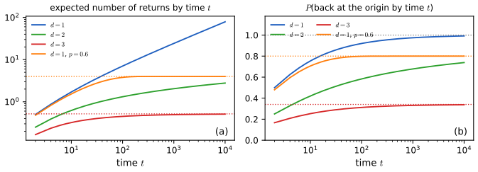
fig_23_s2. Download: PDF · SVGConvergence of Markov chains
p. 390 Started at \(X_0=i\), the recurrence time (first passage time) to \(j\) is
\[ T_{ij}=\min\{n>0:X_n=j\}, \tag{23.12} \]with \(T_{ij}=\infty\) if the chain never reaches \(j\). The mean recurrence time of a recurrent state is
\[ m_i=\E(T_{ii})=\sum_nnf_{ii}(n), \tag{23.13} \]with \(f_{ij}(n)=\P(T_{ij}=n)\) the first-passage probabilities above. A recurrent state is null if \(m_i=\infty\) and positive (non-null) if \(m_i<\infty\). The symmetric random walk on \(\Z\) is null recurrent: it returns surely, but \(\P_0(T_{00}>2n)\)
Lemma 23.19 and Lemma 23.20 p. 390
23.19. If \(i\) is null recurrent, then \(p_{ii}(n)\to0\). 23.20. In a finite chain every recurrent state is positive. (Proofs: Filling the gap 23.9 for 23.20 and 23.12 for 23.19, which uses the coupling of Theorem 23.25.)
The key to both lemmas, and to the convergence theorem, is that positive recurrence is the same thing as having a stationary distribution (Definition 23.23 below), with an explicit formula.
Theorem 23.D (stationary distributions and mean return times)
Let the chain be irreducible.
- If it is recurrent, fix a state \(i\) and let \(\nu_j\)
\({}=\E_i\big[\#\{0\le n<T_{ii}:X_n=j\}\big]\), the expected number of visits to \(j\) during one excursion from \(i\). Then \(\nu\Pm=\nu\), \(\nu_i=1\), \(0<\nu_j<\infty\) for all \(j\), and \(\sum_j\nu_j=m_i\). - (Kac) If \(\pi\) is a stationary distribution, then the chain is recurrent and \(\pi_j=1/m_j\) for every \(j\). In particular \(\pi\) is unique and all states are positive recurrent.
- Hence an irreducible chain has a stationary distribution if and only if it is positive recurrent (one state positive recurrent is enough), and then \(\pi_j=\nu_j/m_i=1/m_j\).
Filling the gap 23.8: proof of Theorem 23.D pp. 390–391
The theorem is what the book's sequence "recurrent, non-null, aperiodic" is for: non-null is exactly the condition for an equilibrium to exist. The proof uses only the Markov property at fixed times. For the weather chain it gives \(m_{\text{sunny}}=7/4\) and \(m_{\text{cloudy}}=7/3\), and for Exercise 23.6 \(m=(13,\,1.6,\,104/31)\); the code computes the mean return times from the first-passage probabilities and finds exactly \(1/\pi_j\).
Proof
(1) Invariance. Write \(T=T_{ii}\) and \(\nu_j=\sum_{n\ge0}\P_i(X_n=j,T>n)\). The event \(\{T>n\}\) is determined by \(X_0,\dots,X_n\), so by Theorem 23.B,
\[ \sum_k\nu_kp_{kj}=\sum_{n\ge0}\sum_k\P_i(X_n=k,T>n)p_{kj}=\sum_{n\ge0}\P_i(X_{n+1}=j,T>n)=\sum_{n\ge1}\P_i(X_n=j,T\ge n). \]For \(j\ne i\), \(\{X_n=j,T\ge n\}=\{X_n=j,T>n\}\) and the \(n=0\) term of \(\nu_j\) is 0, so the sum is \(\nu_j\). For \(j=i\), \(\{X_n=i,T\ge n\}=\{T=n\}\) and the sum is \(\P_i(T<\infty)=1=\nu_i\) (recurrence). Finite and positive: by irreducibility pick \(r,s\) with \(p_{ji}(r)>0\), \(p_{ij}(s)>0\); \(\nu=\nu\Pm^r=\nu\Pm^s\) gives \(1=\nu_i\ge\nu_jp_{ji}(r)\) and \(\nu_j\ge\nu_ip_{ij}(s)>0\). Total mass: \(\sum_j\nu_j\)
(2) Recurrence. First \(\pi_j>0\) for all \(j\): pick \(k\) with \(\pi_k>0\) and \(n\) with \(p_{kj}(n)>0\); \(\pi_j\)
and \(\P_\pi(X_0=j,T\ge1)=\pi_j=1-a_1\). Summing over \(n=1,\dots,N\) telescopes to \(1-a_N\). As \(N\to\infty\), \(a_N\to\P_\pi(\text{never at }j)=0\), because in an irreducible recurrent chain every state is reached from every start (\(f_{kj}=1\), Filling the gap 23.6(5)). Hence \(\pi_j\E_j(T_{jj})\)
(3) If \(i\) is positive recurrent, \(\pi=\nu/m_i\) is a stationary distribution by (1) (the chain is recurrent by Theorem 23.16(1)); by (2) it is the only one and \(m_j=1/\pi_j<\infty\) for all \(j\). Conversely (2) shows that a stationary distribution forces positive recurrence. ∎
p. 390 Periodicity. The chain with \(\Pm=\begin{pmatrix}0&1&0\\0&0&1\\1&0&0\end{pmatrix}\) moves \(1\to2\to3\to1\) deterministically. The period of state \(i\) is \(d(i)=\gcd\{n\ge1:p_{ii}(n)>0\}\); \(i\) is periodic if \(d(i)>1\) and aperiodic if \(d(i)=1\). Here every state has period 3 (the book says the chain started at 1 is in state 3 at times 3, 6, 9; it is in state 1 then: see the notes on the book). A state that can never return has no period. A state with \(p_{ii}>0\) is aperiodic.
Lemma 23.21 (period is a class property) p. 390
If \(i\) has period \(d\) and \(i\lra j\), then \(j\) has period \(d\).
Definitions 23.22 to 23.24 (ergodic, stationary, limiting distribution) pp. 390–391
23.22. A state is ergodic if it is recurrent, non-null and aperiodic; a chain is ergodic if all its states are.
23.23. A probability vector \(\pi\) is a stationary (invariant) distribution if \(\pi=\pi\Pm\). Then \(X_0\sim\pi\) implies \(X_n\sim\pi\Pm^n=\pi\) for every \(n\): once in distribution \(\pi\), the chain stays there.
23.24. The chain has a limiting distribution \(\pi\) if \(\lim_{n\to\infty}p_{ij}(n)=\pi_j\) for all \(i,j\): every row of \(\Pm^n\) converges to the same \(\pi\).
Filling the gap 23.9: proofs of Lemmas 23.20 and 23.21 p. 390
Proofs
Lemma 23.20. A recurrent state \(i\) of a finite chain lies in a closed irreducible class \(C\) (Theorem 23.17), on which the chain is irreducible and recurrent. The vector \(\nu\) of Theorem 23.D(1) has finitely many entries, each finite, so \(m_i=\sum_{j\in C}\nu_j<\infty\).
Lemma 23.21. Pick \(r,s\) with \(p_{ij}(r)>0\), \(p_{ji}(s)>0\). Then \(p_{ii}(r+s)>0\), so \(d(i)\mid r+s\). If \(p_{jj}(n)>0\), then \(p_{ii}(r+n+s)\)
Filling the gap 23.10: aperiodic means eventually positive
Number-theoretic lemma. If a set \(S\) of positive integers is closed under addition and \(\gcd S=1\), then \(S\) contains every sufficiently large integer.
Consequence. If the chain is irreducible and aperiodic, then for all \(i,j\) there is \(N_{ij}\) with \(p_{ij}(n)>0\) for all \(n\ge N_{ij}\). For a finite chain some power \(\Pm^m\) has all entries positive, the hypothesis under which the companion course proves geometric convergence (Result 11.17).
Proof
The gcd of \(S\) is the gcd of some finite subset \(\{n_1,\dots,n_r\}\) (the gcd of the first \(k\) elements decreases and stabilises). Bézout gives integers \(c_k\) with \(\sum c_kn_k=1\); putting the positive and negative terms on two sides, \(1=a-b\) with \(a,b\) in \(S\cup\{0\}\) (positive integer combinations of elements of \(S\) lie in \(S\)). If \(b=0\), \(1\in S\) and we are done. Otherwise, for \(n\ge b^2\) write \(n=qb+r\) with \(0\le r<b\le q\); then \(n=qb+r(a-b)=(q-r)b+ra\) with \(q-r\ge0\), an element of \(S\).
For the chain: \(S_i=\{n\ge1:p_{ii}(n)>0\}\) is closed under addition (Chapman-Kolmogorov) and has gcd 1, so \(p_{ii}(n)>0\) for \(n\ge N_i\). With \(p_{ij}(r)>0\), \(p_{ij}(n)\ge p_{ii}(n-r)p_{ij}(r)>0\) for \(n\ge N_i+r\). For finitely many states take the largest \(N_{ij}\). ∎
Theorem 23.25 (convergence and the ergodic theorem) p. 391
An irreducible, ergodic Markov chain has a unique stationary distribution \(\pi\), its limiting distribution exists and equals \(\pi\), and for every bounded function \(g\), with probability one,
\[ \lim_{N\to\infty}\frac1N\sum_{n=1}^Ng(X_n)=\E_\pi(g)\equiv\sum_jg(j)\pi_j. \tag{23.14} \]More precisely, for every initial distribution, \(\TV(\mu_n,\pi)\)
Filling the gap 23.11: a coupling proof of Theorem 23.25, and the ergodic theorem p. 391
Existence and uniqueness of \(\pi\) are Theorem 23.D(3): the chain is irreducible and positive recurrent.
The coupling. Run two independent copies, \(X\) from \(\mu_0\) and \(Y\) from \(\pi\), until the first time \(T\) at which they are in the same state, and from then on move them together. After \(T\) the two have the same position, and \(Y\) is always distributed as \(\pi\), so for every set \(A\)
\[ |\P(X_n\in A)-\pi(A)|=|\P(X_n\in A)-\P(Y_n\in A)|\le\P(X_n\ne Y_n)\le\P(T>n). \]This is the coupling inequality, \(\TV(\mu_n,\pi)\le\P(T>n)\). It remains to see that \(T<\infty\) almost surely, and this is where aperiodicity enters: the pair \((X_n,Y_n)\) is a Markov chain on \(\Xc\times\Xc\) which, thanks to Filling the gap 23.10, is irreducible, and which has the stationary distribution \(\pi\otimes\pi\); by Theorem 23.D it is recurrent, so it hits the diagonal. In the periodic 3-cycle the two copies started in different states move in parallel and never meet, and the convergence indeed fails (Example 23.27). Figure 23.S1(c) and the demo show \(\P(T>n)\) and \(\TV(\mu_n,\pi)\) side by side.
The ergodic theorem. Cut the path at the successive visits to a fixed state \(i\). The pieces (excursions) are iid by the strong Markov property; each has mean length \(m_i\) and contains on average \(\nu_j=m_i\pi_j\) visits to \(j\). The strong law of large numbers applied to the excursion lengths and to the sums of \(g\) over excursions gives \((23.14)\).
Proof
The product chain. \(Z_n=(X_n,Y_n)\) with \(X,Y\) independent chains is a Markov chain with transition probabilities \(p_{ik}p_{jl}\) from \((i,j)\) to \((k,l)\) and \(n\)-step probabilities \(p_{ik}(n)p_{jl}(n)\). By Filling the gap 23.10 these are positive for all large \(n\), so \(Z\) is irreducible; \(\sum_{i,j}\pi_i\pi_jp_{ik}p_{jl}\)
The coupled chain has the right law. Define \(X'_n=X_n\) for \(n\le T\) and \(X'_n=Y_n\) for \(n>T\). \(T\) is a stopping time for \(Z\). By the strong Markov property (Theorem 23.C for \(Z\)), given the past up to \(T\) and \(Z_T=(k,k)\), the future \((Z_{T+m})\) is a product chain from \((k,k)\), whose two coordinates are each \(\Pm\)-chains from \(k\). So after \(T\), both \((X_{T+m})\) and \((X'_{T+m})=(Y_{T+m})\) are \(\Pm\)-chains from \(X_T\), independent of the past: \(X'\) and \(X\) have the same law (compute the probability of any path by splitting on the value of \(T\)). Therefore \(\P(X_n\in A)=\P(X'_n\in A)\) and the coupling inequality holds as displayed, because \(X'_n=Y_n\) when \(T\le n\).
Limits. \(\P(T>n)\to0\), so \(\TV(\mu_n,\pi)\to0\); with \(\mu_0=\delta_i\), \(p_{ij}(n)\to\pi_j\). Uniqueness again: any stationary \(\pi'\) satisfies \(\pi'_j=\sum_i\pi'_ip_{ij}(n)\to\pi_j\) by dominated convergence.
Ergodic theorem. Let \(\tau_0<\tau_1<\cdots\) be the successive times at \(i\) (all finite, since the chain is irreducible and recurrent), \(L_k=\tau_{k+1}-\tau_k\) and \(G_k\)
which is \(o(N)\). Dividing by \(N\): \(\frac1N\sum_{n\le N}g(X_n)\)
Rates. For a finite chain, \(\P(T>n)\) decays geometrically (the pair chain must hit the diagonal within a fixed number of steps with probability bounded below), which gives \(\TV(\mu_n,\pi)\le C\rho^n\); the companion course derives the explicit Doeblin bound (Result 11.17). The true rate is the largest modulus of an eigenvalue of \(\Pm\) other than 1: 0.4 for the weather chain, 0.35 for Exercise 23.6, 0.5 for Example 23.29.
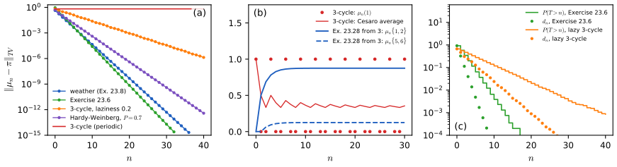
fig_23_s1. Download: PDF · SVGFilling the gap 23.12: proof of Lemma 23.19 (null recurrence means \(p_{ii}(n)\to0\)) p. 390
Two cases, for the class of \(i\) taken as an irreducible chain, first assumed aperiodic. If the product chain \(Z\) of Filling the gap 23.11 is transient, then \(\sum_np_{ii}(n)^2\)
p. 391 Detailed balance. \(\pi\) satisfies detailed balance if
\[ \pi_ip_{ij}=p_{ji}\pi_j\quad\text{for all }i,j. \tag{23.15} \]Theorem 23.26 (detailed balance implies stationarity) p. 391
If \(\pi\) satisfies detailed balance, then \(\pi\Pm=\pi\).
Proof
\((\pi\Pm)_j\)
Filling the gap 23.13: what detailed balance means: reversibility pp. 391–392
Run a chain in its stationary distribution, \(X_0\sim\pi\) with \(\pi_i>0\), and look at it backwards, \(Y_n=X_{N-n}\) for \(0\le n\le N\). Then \(Y\) is a Markov chain with stationary law \(\pi\) and transition probabilities
\[ p^*_{ij}=\frac{\pi_jp_{ji}}{\pi_i}. \]So the reversed chain has the same law as the forward one (the chain is reversible: a film of it cannot be told from the film run backwards) exactly when \(p^*=p\), which is detailed balance. Detailed balance is sufficient for stationarity but not necessary: in Exercise 23.6, \(\pi_1p_{13}=0.0077\) while \(\pi_3p_{31}=0.0149\), so that chain is stationary under \(\pi\) without being reversible (in equilibrium a net probability flow of 0.0072 per step circulates \(1\to2\to3\to1\)); the code estimates \(p^*\) from a reversed simulated path and finds the formula above. Every chain on a path graph (only \(p_{i,i\pm1}\) and \(p_{ii}\) non-zero, like Example 23.7 and Example 23.29) that has a stationary distribution satisfies detailed balance, because the net flow across each edge must be zero. Detailed balance is the design principle of Markov chain Monte Carlo (Example 23.30): it is a local condition, checkable pair by pair without knowing the normalising constant.
Proof
By stationarity and Theorem 23.B(2), \(\P(Y_0=y_0,\dots,Y_n=y_n)\)
Example 23.27 (a stationary distribution without convergence) p. 392
For the 3-cycle, \(\pi=(1/3,1/3,1/3)\) satisfies \(\pi\Pm=\pi\), and a chain started from \(\pi\) stays uniform. But from state 1 the law \(\mu_n\) cycles through the three point masses and has no limit: \(\TV(\mu_n,\pi)=2/3\) for all \(n\). What does survive is the average: \(\frac1N\sum_{n<N}\mu_n\to\pi\), and the ergodic theorem \((23.14)\) holds, since its proof did not use aperiodicity. The fix in practice is laziness: \(\varepsilon I+(1-\varepsilon)\Pm\) has the same stationary distributions and is aperiodic. Exercise 23.9 is the two-state version.
Examples of Markov chains
Example 23.28 p. 392
On \(\{1,\dots,6\}\) with rows \((\tfrac12,\tfrac12,0,0,0,0)\), \((\tfrac14,\tfrac34,0,0,0,0)\), \((\tfrac14,\tfrac14,\tfrac14,\tfrac14,0,0)\), \((\tfrac14,0,\tfrac14,\tfrac14,0,\tfrac14)\), \((0,0,0,0,\tfrac12,\tfrac12)\), \((0,0,0,0,\tfrac12,\tfrac12)\): \(C_1=\{1,2\}\) and \(C_2=\{5,6\}\) are closed irreducible sets; 3 and 4 are transient (the path \(3\to4\to6\) leaves for good); every state has \(p_{ii}>0\), so all are aperiodic. States 1, 2, 5, 6 are ergodic.
Filling the gap 23.14: where Example 23.28 ends up
The chain has two stationary distributions supported on the closed classes, \((\tfrac13,\tfrac23,0,0,0,0)\) and \((0,0,0,0,\tfrac12,\tfrac12)\), and every mixture of them is stationary: with two closed classes, uniqueness fails. Started at a transient state, the chain converges to a mixture whose weights are the absorption probabilities: with \(h_k=\P_k(\text{absorbed in }C_2)\), first-step analysis gives
\[ h_3=\tfrac14h_3+\tfrac14h_4,\qquad h_4=\tfrac14h_3+\tfrac14h_4+\tfrac14, \]so \(h_3=1/8\), \(h_4=3/8\), and from state 3, \(\mu_n\)
Derivation
Condition on the first step (Theorem 23.B): from 3 the chain goes to \(\{1,2\}\) (then \(h=0\)) with probability \(1/2\), stays at 3 or moves to 4 with probability \(1/4\) each. From 4: to 1 (\(h=0\)), 3, 4, or 6 (\(h=1\)) with \(1/4\) each. The first equation gives \(h_4=3h_3\); the second then gives \(\tfrac34\cdot3h_3=\tfrac14h_3+\tfrac14\), so \(h_3=1/8\). Within \(C_1\), \(\pi_1\cdot\tfrac12=\pi_2\cdot\tfrac14\) gives \((1/3,2/3)\). For \(f_{33}\): returning to 3 needs either a loop (\(1/4\)) or a move to 4 followed by an eventual return; from 4 the probability of reaching 3 is \(g=\tfrac14+\tfrac14g\), \(g=1/3\), so \(f_{33}\)
Example 23.29 (Hardy-Weinberg) pp. 392–393
Genotypes AA, Aa, aa have population fractions \((p,q,r)\). If every parent passes one of its two genes at random and mates are chosen at random, the pool of genes has a fraction \(P=p+q/2\) of A and \(Q=r+q/2\) of a, children are AA, Aa, aa with probabilities \((P^2,2PQ,Q^2)\), and the fraction of A among them is \(P^2+PQ=P(P+Q)=P\): the gene frequencies are stable and the genotype frequencies are \((P^2,2PQ,Q^2)\) from the second generation on (the Hardy-Weinberg law). Following one line of descent (one child per generation), the genotype of the \(n\)th descendant is a Markov chain on (AA, Aa, aa) with
\[ \Pm=\begin{pmatrix}P&Q&0\\P/2&1/2&Q/2\\0&P&Q\end{pmatrix},\qquad\pi=(P^2,\,2PQ,\,Q^2). \](The book's middle entry is \((P+Q)/2\), which is \(1/2\).) The same equilibrium is the null model of Section 2.7.2 of Statistical Methods for Modern Biology.
Filling the gap 23.15: the Hardy-Weinberg transition matrix, and convergence in one generation's halving
The child receives one gene from its parent in the line (each of the parent's two genes with probability \(1/2\)) and one from a random mate, which is A with probability \(P\). From AA the child gets A from the parent: AA with probability \(P\), Aa with \(Q\). From aa: Aa with \(P\), aa with \(Q\). From Aa: the parent passes A or a with probability \(1/2\) each, so AA with \(P/2\), aa with \(Q/2\), Aa with \(Q/2+P/2=1/2\). The chain is a path graph, so its stationary distribution satisfies detailed balance (Filling the gap 23.13): \(P^2\cdot Q=2PQ\cdot P/2\) and \(2PQ\cdot Q/2=Q^2\cdot P\), which confirms \(\pi=(P^2,2PQ,Q^2)\) by Theorem 23.26. The eigenvalues of \(\Pm\) are \(1\), \(1/2\) and \(0\), so the distance to equilibrium halves each generation (Figure 23.S1(a), with \(P=0.7\); demo chain "Hardy-Weinberg").
Example 23.30 (Markov chain Monte Carlo) p. 393
To sample from a density \(f=cg\) with \(g\) known and \(c\) unknown, start anywhere and, from \(X_i\), propose \(W\sim\N(X_i,b^2)\), accept it (\(X_{i+1}=W\)) with probability \(r=\min\{g(W)/g(X_i),1\}\), and otherwise stay (\(X_{i+1}=X_i\)). Under weak conditions \(X_0,X_1,\dots\) is an ergodic chain with stationary density \(f\), so by \((23.14)\) averages along the path estimate expectations under \(f\), although \(c\) is never computed.
Filling the gap 23.16: why \(f\) is stationary for the Metropolis chain p. 393
On a continuous state space, detailed balance reads \(f(x)k(x,y)=f(y)k(y,x)\) for the density \(k(x,y)\) of moves \(x\to y\ne x\). For the random-walk Metropolis chain, \(k(x,y)=\phi_b(y-x)\min\{g(y)/g(x),1\}\) with \(\phi_b\) the \(\N(0,b^2)\) density, so
\[ f(x)k(x,y)=c\,\phi_b(y-x)\min\{g(y),g(x)\}, \]which is symmetric in \(x\) and \(y\) because \(\phi_b\) is. Let \(a(x)=\int k(x,y)\d y\) be the acceptance probability from \(x\). For a set \(B\), the chain from \(X_i\sim f\) lands in \(B\) either by an accepted move or by staying:
\[ \P(X_{i+1}\in B)=\int_B\Big[\int f(x)k(x,y)\d x\Big]\d y+\int_Bf(y)(1-a(y))\d y. \]By symmetry the inner integral is \(\int f(y)k(y,x)\d x=f(y)a(y)\), so the total is \(\int_Bf\): \(f\) is stationary. The constant \(c\) cancels from the ratio. The book's Chapter 24 develops this; the companion course proves the general Metropolis-Hastings case (Result 11.19). The code runs the chain for \(g(x)=e^{-x^2/2-x^4/10}\) and recovers \(\E_f(X^2)=0.6155\) (computed by quadrature) to two decimals from \(10^5\) steps.
Inference for Markov chains
p. 394 Observe \(X_0,X_1,\dots,X_n\) from a chain on \(\{1,\dots,N\}\) with unknown \(\mu_0\) and \(\Pm\). Let \(n_{ij}\) be the number of observed transitions \(i\to j\) and \(n_i=\sum_jn_{ij}\). By Theorem 23.B(2) the likelihood is
\[ \mathcal L(\mu_0,\Pm)=\mu_0(x_0)\prod_{r=1}^np_{x_{r-1}x_r}=\mu_0(x_0)\prod_{i=1}^N\prod_{j=1}^Np_{ij}^{n_{ij}}. \]There is a single observation on \(\mu_0\), so it cannot be estimated; maximising over \(\Pm\) (rows nonnegative, summing to one) gives
\[ \hat p_{ij}=\frac{n_{ij}}{n_i}\qquad(n_i>0;\ \hat p_{ij}=0\text{ by convention if }n_i=0). \]Each row is estimated like a multinomial, from the transitions out of that state. This is the counting estimate of the DNA transition matrices in Section 2.8 of Statistical Methods for Modern Biology.
Theorem 23.31 (consistency and asymptotic normality of the MLE) p. 394
Assume the chain is irreducible and ergodic (the book says only ergodic; see the notes on the book). Let \(\hat p_{ij}(n)\) be the MLE after \(n\) transitions and \(N_i(n)=\sum_{r=1}^n\ind(X_r=i)\). Then \(\hat p_{ij}(n)\to p_{ij}\) in probability (indeed almost surely), and the matrix \(\big(\sqrt{N_i(n)}(\hat p_{ij}-p_{ij})\big)_{ij}\) converges in distribution to a Normal matrix with covariances
\[ \Sigma_{ij,k\ell}=\begin{cases}p_{ij}(1-p_{ij})&(i,j)=(k,\ell)\\-p_{ij}p_{i\ell}&i=k,\ j\ne\ell\\0&\text{otherwise.}\end{cases} \]Rows are asymptotically independent, and each row behaves like a multinomial proportion with \(N_i\) trials (Theorem 14.6). Since \(N_i(n)/n\to\pi_i\), the standard error of \(\hat p_{ij}\) is about \(\sqrt{p_{ij}(1-p_{ij})/(n\pi_i)}\), and a Wald interval is \(\hat p_{ij}\pm z_{\alpha/2}\sqrt{\hat p_{ij}(1-\hat p_{ij})/N_i}\).
Filling the gap 23.17: the MLE, and a proof of Theorem 23.31 by "stacks of successors" p. 394
The maximiser. The log-likelihood in \(\Pm\) is \(\sum_i\big[\sum_jn_{ij}\log p_{ij}\big]\), a sum of separate problems, one per row; row \(i\) is the multinomial log-likelihood with counts \(n_{i1},\dots,n_{iN}\), maximised at \(n_{ij}/n_i\) (Theorem 14.5; directly: \(\sum_jn_{ij}\log(p_{ij}/\hat p_{ij})\)
Stacks of successors. Build the chain differently: for each state \(i\) prepare an infinite stack of cards \(\xi_{i1},\xi_{i2},\dots\), iid with law \(p_{i\cdot}\), the stacks independent. At the \(k\)th visit to \(i\), move to the state on card \(\xi_{ik}\). This is a Markov chain with transition matrix \(\Pm\) (each move uses a fresh card independent of the past). In this construction \(n_{ij}\) is the number of \(j\)'s among the first \(N_i\) cards of stack \(i\), so \(\hat p_{i\cdot}\) is the empirical distribution of the first \(N_i\) cards: an iid multinomial sample with a random sample size.
Proof of Theorem 23.31
Consistency. By the ergodic theorem with \(g=\ind_{\{i\}}\), \(N_i(n)/n\to\pi_i>0\) almost surely (irreducibility makes \(\pi_i>0\); without it, a state in another closed class may never be visited and \(\hat p_{ij}\) stays at its conventional value). So \(N_i(n)\to\infty\), and the strong law for the cards of stack \(i\) gives \(\hat p_{ij}\to p_{ij}\) almost surely.
Normality. For a fixed number \(k\) of cards, the CLT for multinomial proportions gives \(\sqrt k(\bar\xi_{i,k}-p_{i\cdot})\rightsquigarrow\N(0,\Sigma_i)\) with \(\Sigma_i\)
What the normalisation by \(N_i\) matters for. Using \(n\) instead of \(N_i\) in the standard error understates it by the factor \(\sqrt{\pi_i}\): in Figure 23.S4(b) (Exercise 23.4's chain, \(\pi_1=0.75\)) the correct interval covers about 95% once \(n\ge200\), the wrong one about 91%.
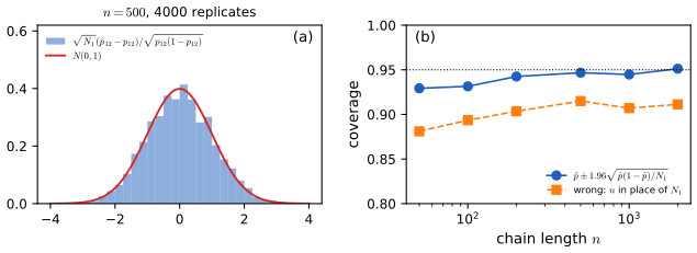
fig_23_s4. Download: PDF · SVG23.3 Poisson Processes
pp. 394–395 Counting events in time (accidents, decays, arriving messages) leads to the Poisson process. Three facts about the Poisson law are used throughout: if \(X\sim\Pois(\lambda)\) then \(\E X=\V X=\lambda\); if \(X\sim\Pois(\lambda)\) and \(Y\sim\Pois(\nu)\) are independent, \(X+Y\sim\Pois(\lambda+\nu)\); and if \(N\sim\Pois(\lambda)\) and \(Y\given N=n\sim\Bin(n,p)\), then \(Y\sim\Pois(\lambda p)\).
Filling the gap 23.18: the three Poisson facts, and a stronger form of the last p. 395
The probability generating function \(G_X(z)=\E z^X=e^{\lambda(z-1)}\) determines the law (its Taylor coefficients at 0 are the probabilities). Means and variances: Filling the gap 3.4. Sums: \(G_{X+Y}=G_XG_Y=e^{(\lambda+\nu)(z-1)}\). Thinning a Poisson count, in the stronger form needed below: if \(N\sim\Pois(\lambda)\) and, given \(N=n\), \((Y_1,\dots,Y_k)\) is multinomial\((n;p_1,\dots,p_k)\), then \(Y_1,\dots,Y_k\) are independent with \(Y_l\sim\Pois(\lambda p_l)\). With \(k=2\) this gives the book's statement and adds that the kept and the discarded counts are independent.
Proof of the multinomial splitting
For \(y_1,\dots,y_k\ge0\) with \(n=\sum y_l\), \(\P(Y=y)\)
p. 395 Let \(X(t)\) be the number of events in \([0,t]\). \(\{X(t):t\ge0\}\) is a counting process, with state space \(\{0,1,2,\dots\}\). Write \(f(h)=o(h)\) if \(f(h)/h\to0\) as \(h\to0\).
Definition 23.32 (Poisson process) p. 395
A counting process \(\{X(t):t\ge0\}\) is a Poisson process with intensity function \(\lambda(t)\ge0\) if
- \(X(0)=0\);
- for any \(0=t_0<t_1<\dots<t_n\) the increments \(X(t_1)-X(t_0),\dots,X(t_n)-X(t_{n-1})\) are independent;
- as \(h\downarrow0\), \[ \P(X(t+h)-X(t)=1)=\lambda(t)h+o(h), \tag{23.16} \] \[ \P(X(t+h)-X(t)\ge2)=o(h). \tag{23.17} \]
In words: in a short interval an event occurs with probability about \(\lambda(t)h\), and two events almost never do. Below, \(\lambda\) is taken continuous and the \(o(h)\) terms uniform for \(t\) in bounded intervals, a regularity the book leaves implicit and which holds in every example.
Theorem 23.33 (counts are Poisson) p. 395
For a Poisson process with intensity \(\lambda(t)\), \(X(s+t)-X(s)\)
Filling the gap 23.19: proof of Theorem 23.33 by a differential equation p. 395
Fix \(s\) and \(z\in[0,1]\), and let \(G(t)=\E z^{X(s+t)-X(s)}\). Independent increments turn the infinitesimal conditions into a differential equation for \(G\):
\[ G'(t)=\lambda(s+t)(z-1)\,G(t),\quad G(0)=1\quad\Longrightarrow\quad G(t)=\exp\{(z-1)(m(s+t)-m(s))\}, \]the generating function of \(\Pois(m(s+t)-m(s))\).
Proof
Write \(D=X(s+t+h)-X(s+t)\). By independent increments, \(G(t+h)=G(t)\,\E z^D\). Since \(0\le z\le1\),
\[ \E z^D=\P(D=0)+z\P(D=1)+\E[z^D;D\ge2]=1-\lambda(s+t)h+z\lambda(s+t)h+o(h), \]using \(\P(D=0)=1-\P(D=1)-\P(D\ge2)\) and \(0\le\E[z^D;D\ge2]\le\P(D\ge2)=o(h)\). So \((G(t+h)-G(t))/h\)
Definition 23.34 (homogeneous Poisson process) p. 396
If \(\lambda(t)\equiv\lambda>0\), the process is homogeneous with rate \(\lambda\), and \(X(t)\sim\Pois(\lambda t)\). The waiting times are \(W_0=0\) and \(W_n=\) the time of the \(n\)th event; the sojourn (interarrival) times are \(S_n=W_{n+1}-W_n\), \(n\ge0\).
Theorem 23.35 (exponential gaps, gamma waiting times) p. 396
For a homogeneous Poisson process with rate \(\lambda\), \(S_0,S_1,\dots\) are iid with density \(\lambda e^{-\lambda s}\), \(s\ge0\) (mean \(1/\lambda\)), and \(W_n\sim\Gam(n,1/\lambda)\), with density
\[ f(w)=\frac{\lambda^n}{\Gamma(n)}w^{n-1}e^{-\lambda w},\quad w>0, \]so \(\E W_n=n/\lambda\) and \(\V W_n=n/\lambda^2\). (The book's density ends in \(e^{-\lambda t}\), a slip for \(e^{-\lambda w}\).)
Filling the gap 23.20: a rigorous proof of Theorem 23.35 p. 396
The book's proof conditions on \(S_1=s\), an event of probability zero, and then applies independent increments after the random time \(W_1\). Both steps can be avoided by computing the joint law of the waiting times directly from counts in fixed intervals. For \(0\)
So \((W_1,\dots,W_n)\) has density \(\lambda^ne^{-\lambda w_n}\) on \(\{0<w_1<\dots<w_n\}\). The change of variables \(s_0=w_1\), \(s_k=w_{k+1}-w_k\) has Jacobian 1 and turns it into \(\prod_{k=0}^{n-1}\lambda e^{-\lambda s_k}\): the gaps are iid exponential. \(W_n\) is a sum of \(n\) of them, hence \(\Gam(n,1/\lambda)\) (Result 2.20), or integrate \(w_1,\dots,w_{n-1}\) out of the density over \(0<w_1<\dots<w_{n-1}<w\) (volume \(w^{n-1}/(n-1)!\)).
Proof of the box formula
For such disjoint boxes, the event is exactly: no event in \([0,a_1]\), exactly one in \((a_1,b_1]\), none in \((b_1,a_2]\), exactly one in \((a_2,b_2]\), ..., none in \((b_{n-1},a_n]\), at least one in \((a_n,b_n]\). The intervals are disjoint, so by independent increments and Theorem 23.33 the probability is
\[ e^{-\lambda a_1}\cdot\lambda(b_1-a_1)e^{-\lambda(b_1-a_1)}\cdot e^{-\lambda(a_2-b_1)}\cdots e^{-\lambda(a_n-b_{n-1})}\cdot\big(1-e^{-\lambda(b_n-a_n)}\big), \]and the exponents add up to \(-\lambda a_n\). The right-hand integral gives the same value. Such boxes determine the joint distribution on the ordered region (they form a family closed under intersection that generates its Borel sets), so the density is as claimed. The code checks the box formula by simulation. ∎
Theorem 23.E (three equivalent definitions of the homogeneous Poisson process)
For a counting process with \(X(0)=0\), the following are equivalent:
- Definition 23.32 with \(\lambda(t)\equiv\lambda\);
- independent increments, and \(X(t)-X(s)\sim\Pois(\lambda(t-s))\) for \(s<t\);
- the gaps \(S_0,S_1,\dots\) are iid \(\Exp(\lambda)\) (mean \(1/\lambda\)) and \(X(t)=\#\{n\ge1:W_n\le t\}\).
A fourth description, on a fixed window \([0,T]\): draw \(N\sim\Pois(\lambda T)\), then place \(N\) iid Uniform\((0,T)\) points (Theorem 23.F).
Filling the gap 23.21: proof of Theorem 23.E
Proof
(1) \(\Rightarrow\) (2) is Theorem 23.33. (2) \(\Rightarrow\) (3) is the proof in Filling the gap 23.20, which used only (2). (2) \(\Rightarrow\) (1): \(\P(X(h)=1)\)
(3) \(\Rightarrow\) (2): a process satisfying (2) exists: on each window \([k,k+1)\) put \(\Pois(\lambda)\) many uniform points, independently across windows; by the multinomial splitting of Filling the gap 23.18 the counts in disjoint subintervals are independent Poisson, which gives (2). By (2) \(\Rightarrow\) (3), its gaps are iid \(\Exp(\lambda)\). The whole path of a counting process is a function of its gaps, so any process with iid \(\Exp(\lambda)\) gaps has the same finite-dimensional distributions as this one, and therefore satisfies (2). ∎
Theorem 23.F (the order-statistics property)
For a homogeneous Poisson process, conditionally on \(X(T)=n\), the event times \((W_1,\dots,W_n)\) have density \(n!/T^n\) on \(\{0<w_1<\dots<w_n<T\}\): they are distributed as the order statistics of \(n\) iid Uniform\((0,T)\) variables. For an inhomogeneous process the unordered event times are, given \(X(T)=n\), iid with density \(\lambda(t)/m(T)\) on \([0,T]\).
Filling the gap 23.22: proof of Theorem 23.F, and two consequences
Consequences: (a) given \(X(T)=n\), the number of events in a subinterval of length \(\ell\) is \(\Bin(n,\ell/T)\), and the counts in \(k\) equal bins are multinomial with equal probabilities, the null hypothesis of Example 23.36 (and of Exercise 23.12); (b) given \(X(T)=n\), the \(k\)th event time is \(T\) times a \(\mathrm{Beta}(k,n-k+1)\) variable (Result 2.21). Figure 23.S3(c) shows (b) for \(T=10\), \(n=5\), \(k=3\).
Proof
Homogeneous case: repeat the box computation of Filling the gap 23.20 with \(b_n<T\) and the event "exactly one in \((a_n,b_n]\) and none in \((b_n,T]\)": the probability of the boxes together with \(X(T)=n\) is \(\prod_{k=1}^n\lambda(b_k-a_k)\cdot e^{-\lambda T}\), so the joint density of \((W_1,\dots,W_n)\) on \(\{X(T)=n\}\) is \(\lambda^ne^{-\lambda T}\) on the ordered region. Dividing by \(\P(X(T)=n)\)
Theorem 23.G (thinning and superposition)
(a) Thinning. Keep each event of a Poisson process with intensity \(\lambda(t)\) independently with probability \(p(t)\) (depending on the event's time). The kept events and the discarded events form two independent Poisson processes with intensities \(\lambda(t)p(t)\) and \(\lambda(t)(1-p(t))\).
(b) Superposition. The union of the events of independent Poisson processes with intensities \(\lambda_1(t)\) and \(\lambda_2(t)\) is a Poisson process with intensity \(\lambda_1(t)+\lambda_2(t)\).
Algorithm 23.B (simulating an inhomogeneous process by thinning)
If \(\lambda(t)\le\lambda_{\max}\) on \([0,T]\): generate a homogeneous process with rate \(\lambda_{\max}\) by adding \(\Exp(\lambda_{\max})\) gaps, and keep a point at time \(t\) with probability \(\lambda(t)/\lambda_{\max}\). By Theorem 23.G(a) the kept points are a Poisson process with intensity \(\lambda(t)\). The simulated web hits of Figure 23.3 and the inhomogeneous preset of the demo are made this way.
Filling the gap 23.23: proof of Theorem 23.G
Proof
(a) Use Theorem 23.F on \([0,T]\). Given \(X(T)=n\), the events are iid with density \(\lambda(t)/m(T)\), and each is independently kept with probability \(p(t)\). Partition \([0,T]\) into disjoint intervals \(I_1,\dots,I_r\) and classify each event by (interval, kept or not): \(2r\) categories, with probabilities \(\int_{I_l}\lambda p/m(T)\) and \(\int_{I_l}\lambda(1-p)/m(T)\). The \(2r\) counts are multinomial given \(n\), with \(n\sim\Pois(m(T))\), so by Filling the gap 23.18 they are independent Poissons with means \(\int_{I_l}\lambda p\) and \(\int_{I_l}\lambda(1-p)\). That is statement (2) of Theorem 23.E (in its inhomogeneous form) for both processes, jointly with their independence.
(b) For disjoint intervals, the counts of the union are sums of independent Poisson counts, independent across intervals, with means \(\int_I(\lambda_1+\lambda_2)\) (Filling the gap 23.18). ∎
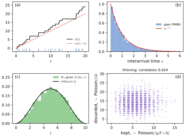
fig_23_s3. Download: PDF · SVGExample 23.36 (hits on a web server) pp. 396–397
The book's Figure 23.3 shows requests to a web server. If they form a homogeneous Poisson process on \([0,T]\), then \(N=X(T)\sim\Pois(\lambda T)\), the likelihood is \(\mathcal L(\lambda)\propto e^{-\lambda T}(\lambda T)^N\), and the MLE is \(\hat\lambda=N/T\) (48.0077 per minute in the book). To test homogeneity, split \([0,T]\) into four equal intervals: given \(N\), each event falls in each interval with probability \(1/4\) under the null, and Pearson's statistic \(\sum_{i=1}^4(O_i-E_i)^2/E_i\) with \(E_i=N/4\) is approximately \(\chi^2_3\) (Theorem 10.17). The book finds \(\chi^2=252\), a p-value near zero: the rate varies in time.
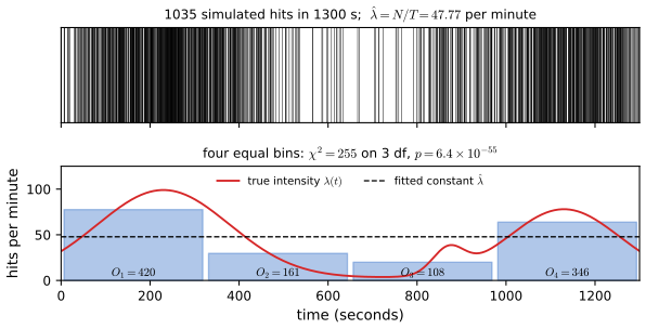
fig_23_3; data: data/ch23-hits.json. Download: PDF · SVGFilling the gap 23.24: the likelihood from the event times, and why the test conditions on \(N\) pp. 396–397
The full likelihood. The data are the event times, not only their number. By the proof of Theorem 23.F, the density of observing exactly the times \(w_1<\dots<w_N\) in \([0,T]\) is \(\lambda^Ne^{-\lambda T}\) for a constant rate, and \(\prod_k\lambda(w_k)\,e^{-m(T)}\) in general. For a constant rate it depends on the data through \(N\) only: \(N\) is sufficient, the book's count likelihood is the full likelihood up to a constant, and \(\hat\lambda=N/T\) (set the derivative of \(N\log\lambda-\lambda T\) to zero; the second derivative \(-N/\lambda^2\) is negative). The standard error is \(\sqrt{\hat\lambda/T}\).
The test. Because \(\lambda\) is unknown, the test conditions on \(N\), which removes it: by Theorem 23.F the bin counts are multinomial\((N;\tfrac14,\dots,\tfrac14)\) under the null, whatever \(\lambda\) is. Pearson's statistic and the likelihood ratio statistic \(G^2=2\sum O_i\log(O_i/E_i)\) both have the \(\chi^2_{k-1}\) limit (Theorem 10.17, Theorem 10.22). Simulating 4000 homogeneous processes, the code finds a rejection rate of 5.05% at the 5% level. The test only looks at the four bin totals: a rate that varies within the bins and averages out across them goes unnoticed, and more bins trade sensitivity to fast variation against power.
Units. The book reports \(\hat\lambda\) per minute while the axis of its figure runs to about 1300 without units. A rate of 48 per minute over 1300 minutes would mean about 62,000 events, for which \(\chi^2=252\) would be a mild 6% departure across bins, at odds with the long empty stretches in the figure; over 1300 seconds (about 22 minutes) it means about 1040 events, consistent with both. The simulated stand-in uses seconds.
23.4 Bibliographic Remarks
p. 397 The book points to Grimmett and Stirzaker (1982), Taylor and Karlin (1994), Guttorp (1995) and Ross (2002), from which its exercises are taken. The generating-function proof of the recurrence criterion and the coupling proof of convergence follow the tradition of Feller (1968) and Doeblin (1938), as presented by Lindvall (1992), Norris (1997) and Levin, Peres and Wilmer (2009), who also treat rates of convergence (mixing times). Pólya (1921) proved the recurrence theorem for lattice walks, and Watson (1939) evaluated the three-dimensional constant. The asymptotics of the transition-probability MLE are due to Anderson and Goodman (1957) and Billingsley (1961). The thinning algorithm for inhomogeneous Poisson processes is Lewis and Shedler (1979); Kingman (1993) is a short book on Poisson processes.
Notes on the book
None of the following is in the author's two errata lists (which have no entries for Chapter 23); each comes with its evidence.
Page 384: the rows of \(\Pm\) sum to one, \(\sum_jp_{ij}=1\), not \(\sum_ip_{ij}=1\)
The book writes \(\sum_ip_{ij}=1\) and in the next sentence says "each row can be regarded as a probability mass function". Rows are indexed by \(i\), so the sum is over \(j\): \(\sum_jp_{ij}\)
Page 390: the 3-cycle started in state 1 is in state 1, not state 3, at times 3, 6, 9
With \(p_{12}=p_{23}=p_{31}=1\), from \(X_0=1\) the path is \(2,3,1,2,3,1,\dots\) at times \(1,2,3,\dots\): the chain is in state 1 at times 3, 6, 9 and in state 3 at times 2, 5, 8. The conclusion (period 3) is unaffected. On the same page, "greater common divisor" should read "greatest common divisor", and in \((23.12)\) "assuming \(X_n\) ever returns to state \(i\)" should read "ever reaches state \(j\)".
Page 387: "\(p_{ij}(n)>0\) for some \(n\)" must allow \(n=0\)
Theorem 23.12(1), \(i\lra i\), fails for states that can never return if only \(n\ge1\) is allowed: in Example 23.7 with \(N=3\), \(p_{22}(n)=0\) for all \(n\ge1\). With the convention \(p_{ii}(0)=1\) (Filling the gap 23.4) the theorem holds.
Page 396, Theorem 23.35: the gamma density should end in \(e^{-\lambda w}\), and the gaps are indexed from \(S_0\)
The density printed as \(\frac1{\Gamma(n)}\lambda^nw^{n-1}e^{-\lambda t}\) is not a density in \(w\); it is \(\frac{\lambda^n}{\Gamma(n)}w^{n-1}e^{-\lambda w}\), as its stated mean \(n/\lambda\) and variance \(n/\lambda^2\) require. Also, with \(S_n=W_{n+1}-W_n\) the first gap is \(S_0=W_1\), while the proof calls the first gap \(S_1\) and the second \(S_2\).
Page 394, Theorem 23.31: the chain must also be irreducible
"Ergodic" (every state recurrent, non-null, aperiodic) allows several closed classes. Example 23.28 restricted to \(\{1,2\}\cup\{5,6\}\) is ergodic, but a chain started in \(\{1,2\}\) never visits 5 or 6, so \(N_5(n)=0\) for ever and \(\hat p_{56}\) stays at its conventional value 0, while \(p_{56}=1/2\): the MLE is not consistent. With irreducibility, \(N_i(n)/n\to\pi_i>0\) for every \(i\) and the theorem holds (Filling the gap 23.17).
Pages 390–391: the ergodic averages (23.14) do not need aperiodicity
Not an error, but worth knowing: Theorem 23.25 assumes an ergodic (in particular aperiodic) chain for all its conclusions, while \((23.14)\) holds for every irreducible positive recurrent chain (Filling the gap 23.11). For the periodic chain of Example 23.27, time averages converge to \(\E_\pi g\) although \(\mu_n\) does not converge. Likewise, in Example 23.29 the matrix entry \((P+Q)/2\) is simply \(1/2\).
23.5 Exercises
All sixteen exercises of Chapter 23 (Wasserman, 2004, pp. 398–401), restated in my own words, with complete solutions (hidden). Simulation results quoted below come from the Python code.
Exercise 23.1. A chain on \(\{0,1,2\}\) has rows \((0.1,0.2,0.7)\), \((0.9,0.1,0.0)\), \((0.1,0.8,0.1)\) and \(\mu_0=(0.3,0.4,0.3)\). Find \(\P(X_0=0,X_1=1,X_2=2)\) and \(\P(X_0=0,X_1=1,X_2=1)\).
Solution
By Theorem 23.B(2), \(\P(X_0=0,X_1=1,X_2=2)\)
\({}=\mu_0(0)p_{01}p_{12}\) \({}=0.3\times0.2\times0.0\) \({}=0\) (state 1 never moves to 2), and \(\P(X_0=0,X_1=1,X_2=1)\) \({}=0.3\times0.2\times0.1\) \({}=0.006\). Exercise 23.2. \(Y_1,Y_2,\dots\) are iid with \(\P(Y=0,1,2,3)=(0.1,0.3,0.2,0.4)\); \(X_0=0\) and \(X_n=\max\{Y_1,\dots,Y_n\}\). Show that \((X_n)\) is a Markov chain and find its transition matrix.
Solution
\(X_{n+1}=\max(X_n,Y_{n+1})\), and \(Y_{n+1}\) is independent of \((X_0,\dots,X_n)\) (a function of \(Y_1,\dots,Y_n\)). So \(\P(X_{n+1}=j\given X_0,\dots,X_n=i)\)
\[ \Pm=\begin{pmatrix}0.1&0.3&0.2&0.4\\0&0.4&0.2&0.4\\0&0&0.6&0.4\\0&0&0&1\end{pmatrix}. \]\({}=\P(\max(i,Y)=j)\), which depends on \(i\) only: a homogeneous chain (the construction of Algorithm 23.A with \(\phi(i,y)=\max(i,y)\)). From \(i\): stay with probability \(\P(Y\le i)\), jump to \(j>i\) with \(\P(Y=j)\): States 0, 1, 2 are transient and 3 is absorbing; a simulation of \(10^5\) sequences reproduces row 2 to within 0.01.
Exercise 23.3. For the two-state chain with \(p_{12}=a\), \(p_{21}=b\), \(0<a,b<1\), prove that every row of \(\Pm^n\) converges to \(\big(\frac b{a+b},\frac a{a+b}\big)\).
Solution
By Filling the gap 23.3, \(\Pm^n=\frac1{a+b}\begin{pmatrix}b&a\\b&a\end{pmatrix}+\frac{(1-a-b)^n}{a+b}\begin{pmatrix}a&-a\\-b&b\end{pmatrix}\). Since \(0<a+b<2\), \(|1-a-b|<1\) and the second term tends to 0 geometrically. (The formula can also be checked by induction: it holds for \(n=1\), and multiplying by \(\Pm\) on the right reproduces it with \(n+1\).) The code compares the formula with matrix powers.
Exercise 23.4. With \(a=0.1\), \(b=0.3\), simulate the chain, plot the proportions \(\hat p_n(1)\), \(\hat p_n(2)\) of time spent in each state against \(n\), and check that they approach the limits of Exercise 23.3.
Solution
The limits are \(b/(a+b)=0.75\) and \(a/(a+b)=0.25\). Figure 23.S5(a) shows one chain of length 20,000 started in state 1: the proportions wander at first (the chain stays about \(1/a=10\) steps in state 1 and \(1/b\approx3.3\) in state 2 per visit) and settle near the limits; at \(n=20{,}000\), \(\hat p_n(1)=0.739\). This is the ergodic theorem \((23.14)\) with \(g=\ind_{\{1\}}\). The fluctuations are larger than for iid sampling, because successive states are positively correlated.
Exercise 23.5 (branching process). Each animal has \(Y\) children, \(\P(Y=k)=p_k\), independently; \(X_n\) is the size of generation \(n\), \(X_0=1\), and \(X_{n+1}=Y^{(n)}_1+\dots+Y^{(n)}_{X_n}\). Let \(\mu=\E Y\), \(\sigma^2=\V Y\), \(M(n)=\E X_n\), \(V(n)=\V X_n\). (a) Show \(M(n+1)=\mu M(n)\) and \(V(n+1)=\sigma^2M(n)+\mu^2V(n)\). (b) Show \(M(n)=\mu^n\) and \(V(n)\)
\({}=\sigma^2\mu^{n-1}(1+\mu+\dots+\mu^{n-1})\). (c) What happens to \(V(n)\) for \(\mu>1\), \(\mu=1\), \(\mu<1\)? (d) With \(N=\min\{n:X_n=0\}\) and \(F(n)=\P(N\le n)\), show \(F(n)=\sum_kp_kF(n-1)^k\). (e) Compute \(F(n)\) for \(p_0=\tfrac14\), \(p_1=\tfrac12\), \(p_2=\tfrac14\). Solution
(a) Given \(X_n=x\), \(X_{n+1}\) is a sum of \(x\) iid copies of \(Y\): \(\E(X_{n+1}\given X_n)=\mu X_n\) and \(\V(X_{n+1}\given X_n)=\sigma^2X_n\). Iterated expectation and the law of total variance (Result 3.12) give \(M(n+1)=\mu M(n)\) and \(V(n+1)\)
\({}=\E(\sigma^2X_n)+\V(\mu X_n)\) \({}=\sigma^2M(n)+\mu^2V(n)\). (b) \(M(0)=1\) gives \(M(n)=\mu^n\). \(V(0)=0\), so \(V(1)=\sigma^2\), matching the formula; if it holds for \(n\), then \(V(n+1)\)
\({}=\sigma^2\mu^n+\mu^2\sigma^2\mu^{n-1}(1+\dots+\mu^{n-1})\) \({}=\sigma^2\mu^n(1+\mu+\dots+\mu^n)\), the formula for \(n+1\). (c) For \(\mu\ne1\), \(V(n)\)
\({}=\sigma^2\mu^{n-1}\frac{\mu^n-1}{\mu-1}\). If \(\mu>1\), \(V(n)\) \({}\sim\frac{\sigma^2}{\mu(\mu-1)}\mu^{2n}\) grows geometrically (the standard deviation grows like the mean \(\mu^n\)); if \(\mu=1\), \(V(n)=n\sigma^2\) grows linearly while the mean stays 1; if \(\mu<1\), \(V(n)\) \({}\sim\frac{\sigma^2}{1-\mu}\mu^{n-1}\) \({}\to0\), as the population dies out. (d) \(\{N\le n\}=\{X_n=0\}\) because 0 is absorbing. Condition on the first parent's \(k\) children: each starts an independent copy of the process, and the whole population is extinct at generation \(n\) exactly when all \(k\) sub-populations are extinct at their generation \(n-1\). So \(F(n)=\sum_kp_kF(n-1)^k=G(F(n-1))\), with \(G(s)=\E s^Y\) and \(F(0)=0\).
(e) \(G(s)=(1+s)^2/4\) (here \(Y\sim\Bin(2,\tfrac12)\), \(\mu=1\), \(\sigma^2=\tfrac12\)). \(F(1)=0.25\), \(F(2)=25/64=0.3906\), \(F(3)=0.4835\), \(F(4)=0.5502\), \(F(5)=0.6008\), \(F(10)=0.7415\), \(F(20)=0.8462\), \(F(50)=0.9296\). \(F(n)\to1\) (the critical process dies out surely; the extinction probability is the smallest root of \(G(s)=s\), here \(s=1\)) but slowly, like \(1-2/(\sigma^2n)=1-4/n\), so \(\E N=\infty\). Figure 23.S5(b) compares the recursion with 20,000 simulated lineages.
Exercise 23.6. Find the stationary distribution of \(\Pm\) with rows \((0.40,0.50,0.10)\), \((0.05,0.70,0.25)\), \((0.05,0.50,0.45)\).
Solution
Solve \(\pi\Pm=\pi\), \(\sum\pi_i=1\). The first column gives \(\pi_1\)
\({}=0.4\pi_1+0.05(\pi_2+\pi_3)\) \({}=0.4\pi_1+0.05(1-\pi_1)\), so \(\pi_1=1/13\). The third column gives \(0.55\pi_3=0.1\pi_1+0.25\pi_2\); with \(\pi_2=12/13-\pi_3\): \(0.8\pi_3=0.1/13+3/13\), \(\pi_3=31/104\), and \(\pi_2=65/104=5/8\). So \(\pi\) \({}=(1/13,\,5/8,\,31/104)\) \({}\approx(0.0769,0.6250,0.2981)\). The chain is irreducible and aperiodic, so this is also its limiting distribution; the mean return times are \(1/\pi=(13,1.6,3.35)\). Exercise 23.7. Show that if \(i\) is recurrent and \(i\lra j\), then \(j\) is recurrent.
Solution
This is Theorem 23.16(1), proved in Filling the gap 23.6: with \(p_{ji}(r)>0\) and \(p_{ij}(s)>0\), \(\sum_np_{jj}(n)\)
\({}\ge p_{ji}(r)p_{ij}(s)\sum_np_{ii}(n)\) \({}=\infty\), and Theorem 23.15 makes \(j\) recurrent. Exercise 23.8. Which states of the chain on \(\{1,\dots,6\}\) with rows \((\tfrac13,0,\tfrac13,0,0,\tfrac13)\), \((\tfrac12,\tfrac14,\tfrac14,0,0,0)\), \((0,0,0,0,1,0)\), \((\tfrac14,\tfrac14,\tfrac14,0,0,\tfrac14)\), \((0,0,1,0,0,0)\), \((0,0,0,0,0,1)\) are transient and which recurrent?
Solution
The moves: \(1\to\{1,3,6\}\), \(2\to\{1,2,3\}\), \(3\to5\), \(4\to\{1,2,3,6\}\), \(5\to3\), \(6\to6\). The classes are \(\{1\}\), \(\{2\}\), \(\{4\}\), \(\{3,5\}\), \(\{6\}\): nothing leads back to 1 or 2 once the chain moves to 3 or 6, and no state leads to 4 (its column is zero). \(\{3,5\}\) (a 2-cycle, period 2) and \(\{6\}\) (absorbing) are closed, hence recurrent; \(\{1\}\), \(\{2\}\), \(\{4\}\) are not closed, hence transient (Filling the gap 23.6(6)). State 4 is never revisited and has no period. The code's classification agrees.
Exercise 23.9. For \(\Pm=\begin{pmatrix}0&1\\1&0\end{pmatrix}\), show that \(\pi=(\tfrac12,\tfrac12)\) is stationary. Does the chain converge?
Solution
\(\pi\Pm=(\tfrac12,\tfrac12)\). But \(\Pm^n=I\) for even \(n\) and \(\Pm\) for odd \(n\), so \(\Pm^n\) has no limit and from a fixed state \(\mu_n\) alternates between the two point masses: the chain has period 2 and is not ergodic (Example 23.27 in two states). What does converge is the average \(\frac1N\sum_{n<N}\Pm^n\to\begin{pmatrix}1/2&1/2\\1/2&1/2\end{pmatrix}\), and time averages along the path converge to \(\tfrac12\) (Filling the gap 23.11).
Exercise 23.10. With \(0<p<1\), \(q=1-p\), the chain on \(\{1,\dots,5\}\) moves from \(k\le4\) to \(k+1\) with probability \(p\) and back to 1 with probability \(q\), and from 5 to 1 surely. Find its limiting distribution.
Solution
The chain is irreducible (\(1\to2\to\dots\to5\to1\)) and aperiodic (\(p_{11}=q>0\)), finite, hence ergodic: the limit is the stationary distribution. For \(k=2,\dots,5\) the only way into \(k\) is from \(k-1\), so \(\pi_k=p\,\pi_{k-1}\) and \(\pi_k=p^{k-1}\pi_1\). Normalising,
\[ \pi_k=\frac{(1-p)\,p^{k-1}}{1-p^5},\qquad k=1,\dots,5. \]The equation for state 1 holds automatically: \(q(\pi_1+\dots+\pi_4)+\pi_5\)
\({}=\pi_1[(1-p)(1+p+p^2+p^3)+p^4]\) \({}=\pi_1\). For \(p=1/2\): \(\pi=(16,8,4,2,1)/31\). Exercise 23.11. \(X(t)\) is a Poisson process with intensity \(\lambda(t)>0\) and \(\Lambda(t)=\int_0^t\lambda(u)\d u\). Define \(Y(s)=X(t)\) where \(s=\Lambda(t)\). Show that \(Y\) is a homogeneous Poisson process with rate 1.
Solution
Since \(\lambda>0\), \(\Lambda\) is continuous and strictly increasing, with a continuous increasing inverse, so \(Y(s)=X(\Lambda^{-1}(s))\) is defined for \(0\le s<\Lambda(\infty)\) (assume \(\Lambda(\infty)=\infty\) for all \(s\)). \(Y(0)=X(0)=0\). Disjoint \(s\)-intervals correspond to disjoint \(t\)-intervals, so increments of \(Y\) over disjoint intervals are increments of \(X\) over disjoint intervals, hence independent. By Theorem 23.33, \(Y(s_2)-Y(s_1)\)
\({}=X(t_2)-X(t_1)\) \({}\sim\Pois(\Lambda(t_2)-\Lambda(t_1))\) \({}=\Pois(s_2-s_1)\). By Theorem 23.E(2), \(Y\) is a rate-1 homogeneous Poisson process. (Read backwards, this is another way to simulate an inhomogeneous process: map unit-rate points through \(\Lambda^{-1}\).) Exercise 23.12. For a Poisson process with rate \(\lambda\), find the conditional distribution of \(X(t)\) given \(X(t+s)=n\).
Solution
For \(0\le k\le n\), by independent increments,
\[ \P(X(t)=k\given X(t+s)=n)=\frac{e^{-\lambda t}\frac{(\lambda t)^k}{k!}\,e^{-\lambda s}\frac{(\lambda s)^{n-k}}{(n-k)!}}{e^{-\lambda(t+s)}\frac{(\lambda(t+s))^n}{n!}}=\binom nk\Big(\frac t{t+s}\Big)^k\Big(\frac s{t+s}\Big)^{n-k}: \]\(\Bin(n,t/(t+s))\), free of \(\lambda\), as the order-statistics property predicts (each of the \(n\) uniform points lands in \([0,t]\) with probability \(t/(t+s)\)). Simulation with \(t=2\), \(s=3\), \(n=6\) matches \(\Bin(6,0.4)\) to within 0.02 in every cell.
Exercise 23.13. For a Poisson process with rate \(\lambda\), find \(\P(X(t)\text{ is odd})\).
Solution
\(\P(\text{odd})\)
\({}=e^{-\lambda t}\sum_{k\text{ odd}}\frac{(\lambda t)^k}{k!}\) \({}=e^{-\lambda t}\sinh(\lambda t)\) \({}=\frac{1-e^{-2\lambda t}}2\). Equivalently, \(\P(\text{even})-\P(\text{odd})\) \({}=\E(-1)^{X(t)}\) \({}=e^{-2\lambda t}\) from the generating function at \(z=-1\). It increases to \(1/2\) as \(t\to\infty\). Exercise 23.14. Users log in according to a Poisson process with rate \(\lambda\), and each stays logged in for an independent random time with cdf \(G\). Find the distribution of the number \(Y(t)\) of users logged in at time \(t\) (nobody is logged in at time 0).
Solution
A user arriving at time \(u\le t\) is still logged in at \(t\) with probability \(1-G(t-u)\). This is thinning with a time-dependent probability (Theorem 23.G(a)): the users still present form a Poisson process (in the arrival-time variable) with intensity \(\lambda(1-G(t-u))\) on \([0,t]\), so
\[ Y(t)\sim\Pois\Big(\lambda\int_0^t\big(1-G(t-u)\big)\d u\Big)=\Pois\Big(\lambda\int_0^t\big(1-G(v)\big)\d v\Big). \]As \(t\to\infty\) the mean tends to \(\lambda\E(\text{session length})\) (the infinite-server queue). Simulation with \(\lambda=3\), \(t=4\) and exponential sessions of mean 2 gives mean and variance both near \(3\cdot2(1-e^{-2})=5.19\).
Exercise 23.15. For a Poisson process with rate \(\lambda\) and waiting times \(W_1,W_2,\dots\), show that \(\E\sum_{i=1}^{X(t)}f(W_i)\)
\({}=\lambda\int_0^tf(w)\d w\) (for integrable \(f\)). Solution
The sum does not depend on the order of the points, so by Theorem 23.F, given \(X(t)=n\) it is distributed as \(\sum_{i=1}^nf(U_i)\) with \(U_i\) iid Uniform\((0,t)\), whose mean is \(n\cdot\frac1t\int_0^tf\). Taking expectations over \(X(t)\sim\Pois(\lambda t)\): \(\lambda t\cdot\frac1t\int_0^tf\)
\({}=\lambda\int_0^tf\) (Campbell's formula). With \(f=\cos\), \(\lambda=2\), \(t=3\), the simulated mean is within 0.03 of \(2\sin3=0.282\). Exercise 23.16. In a planar Poisson process with intensity \(\lambda\) (the number of points in a set \(A\) is \(\Pois(\lambda\,\mathrm{area}(A))\), independent for disjoint sets), let \(X\) be the distance from a fixed point \(x_0\) to the nearest point. Show that \(\P(X>t)=e^{-\lambda\pi t^2}\) and \(\E X=1/(2\sqrt\lambda)\).
Solution
\(X>t\) exactly when the disc of radius \(t\) around \(x_0\) contains no point: probability \(e^{-\lambda\pi t^2}\). Then \(\E X\)
\({}=\int_0^\infty\P(X>t)\d t\) \({}=\int_0^\infty e^{-\lambda\pi t^2}\d t\) \({}=\frac12\sqrt{\frac{\pi}{\lambda\pi}}\) \({}=\frac1{2\sqrt\lambda}\) (half a Gaussian integral). Simulating with \(\lambda=2\) gives a mean within 0.005 of \(0.354\).
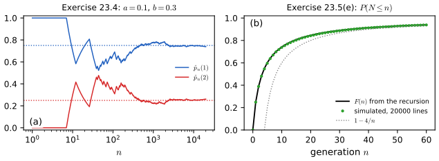
fig_23_s5. Download: PDF · SVGDemonstrations for this chapter
Each demonstration runs in the browser and links back to these notes. The ▶ Demo boxes above open them already set to the case under discussion.
| Demonstration | What you can see | Sections and results |
|---|---|---|
| Convergence to the stationary distribution | The law \(\mu_n\) of a chain from the book (as bars), its classes and periods, the distance to \(\pi\) on a log scale, and the coupling estimate of \(\P(T>n)\); laziness slider. Presets: 1 the weather chain; 2 Exercise 23.6; 3 the periodic 3-cycle; 4 the lazy 3-cycle; 5 Example 23.28. | 23.2; Theorem 23.25, 23.D; Filling the gaps 23.11, 23.14 |
| Recurrence of random walks | Simulated walkers on the line, in the plane and in space; the expected number of returns and the probability of having returned, exactly and by simulation. Presets: 1 the line; 2 a drift; 3 the plane; 4 space; 5 a small drift. | Theorem 23.15; Example 23.18; Filling the gaps 23.5, 23.7 |
| The Poisson process | A process built from exponential gaps, from a Poisson count and uniform times, by thinning, by superposition, or with a varying rate; gaps against the exponential density; the test of homogeneity with \(k\) bins, on one realisation and over replicates; the simulated web hits. Presets: 1 gaps; 2 count then uniform; 3 Example 23.36; 4 thinning; 5 a varying rate. | 23.3; Theorems 23.35, 23.E–23.G; Filling the gap 23.24 |
Related demonstrations in the companion courses: the PageRank demo of Statistical Learning: Theory and Methods (a stationary distribution by power iteration), the MCMC demo and the HMM demo of Bayesian and Probabilistic Machine Learning, and the CpG island demo of Statistical Methods for Modern Biology (transition matrices estimated by counting). The Python code that produces every figure of this page is code/ch23_stochastic_processes.py (see the code index).
References
- Wasserman, L. (2004). All of Statistics: A Concise Course in Statistical Inference. Springer, New York. Chapter 23, pp. 381–401. www.stat.cmu.edu/~larry/all-of-statistics.
- Anderson, T. W. and Goodman, L. A. (1957). Statistical inference about Markov chains. The Annals of Mathematical Statistics, 28(1), 89–110.
- Billingsley, P. (1961). Statistical Inference for Markov Processes. University of Chicago Press, Chicago.
- Doeblin, W. (1938). Exposé de la théorie des chaînes simples constantes de Markov à un nombre fini d'états. Revue mathématique de l'Union interbalkanique, 2, 77–105.
- Feller, W. (1968). An Introduction to Probability Theory and Its Applications, Volume I, 3rd edition. Wiley, New York.
- Grimmett, G. R. and Stirzaker, D. R. (1982). Probability and Random Processes. Oxford University Press, Oxford.
- Guttorp, P. (1995). Stochastic Modeling of Scientific Data. Chapman and Hall, London.
- Kingman, J. F. C. (1993). Poisson Processes. Oxford University Press, Oxford.
- Levin, D. A., Peres, Y. and Wilmer, E. L. (2009). Markov Chains and Mixing Times. American Mathematical Society, Providence.
- Lewis, P. A. W. and Shedler, G. S. (1979). Simulation of nonhomogeneous Poisson processes by thinning. Naval Research Logistics Quarterly, 26(3), 403–413.
- Lindvall, T. (1992). Lectures on the Coupling Method. Wiley, New York.
- Norris, J. R. (1997). Markov Chains. Cambridge University Press, Cambridge.
- Pólya, G. (1921). Über eine Aufgabe der Wahrscheinlichkeitsrechnung betreffend die Irrfahrt im Straßennetz. Mathematische Annalen, 84, 149–160.
- Ross, S. M. (2002). Probability Models, 8th edition. Academic Press, San Diego.
- Taylor, H. M. and Karlin, S. (1994). An Introduction to Stochastic Modeling, revised edition. Academic Press, San Diego.
- Watson, G. N. (1939). Three triple integrals. The Quarterly Journal of Mathematics, 10(1), 266–276.
The numerical statements in the text (the classes and periods of every chain, the stationary distributions, mean return times and absorption probabilities, the first-passage and renewal identities, the exact random-walk return probabilities and Watson's constant, the coupling inequality, the MLE and its sampling distribution, the Poisson box probabilities, order statistics, thinning and superposition, the test of Example 23.36 and the solutions of the exercises) were confirmed numerically.