Estimating the cdf and Statistical Functionals
This is the first chapter of real inference, and it starts with the most general problem there is: estimate an unknown distribution \(F\) from an iid sample, assuming nothing about it. The answer is the empirical distribution function, which puts mass \(1/n\) on each observation. It is unbiased at every point, it converges to \(F\) uniformly (the Glivenko–Cantelli theorem), and the Dvoretzky–Kiefer–Wolfowitz inequality turns it into a confidence band that holds for every \(F\) and every \(n\). Any feature of \(F\) (a mean, a variance, a quantile, a correlation) can then be estimated by evaluating the same feature at the empirical distribution: the plug-in principle. The book states the theorems and leaves the standard errors of most plug-in estimators to the next chapter. These notes prove the theorems, give the standard errors now through the influence function and the delta method, and show by simulation where the resulting Normal intervals can and cannot be trusted.
Ch. 1 Probability Ch. 2 Random variables Ch. 3 Expectation Ch. 4 Inequalities Ch. 5 Convergence Ch. 6 Models and inference Ch. 7 Estimating the CDF Ch. 8 Bootstrap Ch. 9 Parametric inference Ch. 10 Hypothesis testing Ch. 11 Bayesian inference Ch. 12 Decision theory Ch. 13 Regression Ch. 14 Multivariate models Ch. 15 Independence Ch. 16 Causal inference Ch. 17 Directed graphs Ch. 18 Undirected graphs Ch. 19 Log-linear models Ch. 20 Curve estimation Ch. 21 Orthogonal functions Ch. 22 Classification Ch. 23 Stochastic processes Ch. 24 Simulation
How to read these notes
They follow the book. Sections carry the book's numbers (7.1, 7.2, ...) and every displayed equation that appears in the book carries the book's own equation number, e.g. \((7.2)\). Numbered items keep the book's numbers (Definition 7.1, Theorem 7.5, Example 7.13); the confidence band, which the book states in an unnumbered box, is Definition 7.A. Equations without a number are steps that the book skips.
Filling the gaps. Wherever the book says "it can be shown", quotes a theorem without proof, or leaves an argument implicit, an orange Filling the gap box gives the full argument. Proofs and derivations start hidden: open one with its bar, or use the button below.
Figures and demonstrations. Figure 7.1 of the book is reproduced from the nerve data; Figure 7.2 cannot be, because its data are not distributed with the book (Example 7.15). Six supplementary figures (7.S1 to 7.S6) illustrate the gaps filled here; all are computed by the Python code. The ▶ Demo boxes open an interactive demonstration already set to the case being discussed.
Main reference
L. Wasserman, All of Statistics: A Concise Course in Statistical Inference, Springer (2004), Chapter 7, pages 97–105 (book website, with the data sets: www.stat.cmu.edu/~larry/all-of-statistics). Section, equation, example and exercise numbers below refer to this book. Further reading is listed in the references.
The explanations, derivations, figures and code are my own; equations are cited by their numbers in the book.
Companion courses
The empirical distribution function and the plug-in idea appear in several companion courses on this site, at other levels and for other purposes:
- Statistical Methods for Modern Biology, Chapter 3: the empirical CDF as a plot (Section 3.6.7), with uniform convergence, the DKW band and the Kolmogorov–Smirnov distance (Filling the gap 3.7, Result 3.4), and its ECDF and QQ-plot demo; sample quantiles in Section 2.6.1 (Definition 2.4).
- Statistical Learning: Theory and Methods, Chapter 7: the bootstrap, which resamples from \(\Fn\) (Section 7.11), and the Vapnik–Chervonenkis dimension (Section 7.9), whose uniform laws of large numbers generalise the Glivenko–Cantelli theorem from half-lines \((-\infty,x]\) to richer classes of sets; Section 8.2 on the bootstrap against maximum likelihood.
- Applied Statistical Learning in R and Python, Chapter 5: the nonparametric bootstrap standard error, a plug-in estimate computed by simulation (Definition 5.5).
- First-year notes, Estimation and hypothesis testing (advanced): large-sample intervals for a mean (Section 3.2), for proportions (Section 3.5) and for two samples (Section 3.4, Section 9), the Normal-based intervals (7.6) of this chapter in their elementary form.
The companion course proves Glivenko–Cantelli in a few lines and quotes the DKW inequality; here the result is the centre of the chapter, so the proof is given in full (Filling the gap 7.3), together with what is new: the reduction of every \(F\) to the uniform case (7.4), an elementary DKW-type inequality with a complete proof and the reason the constant 2 cannot be improved (7.5), simultaneous against pointwise coverage (7.6), the asymptotic normality of sample quantiles (7.11) and the influence function as the general tool for standard errors (7.12).
The chapter at a glance
- 7.1 The empirical cdf \(\Fn\) (Definition 7.1, Filling the gap 7.1) is, at each \(x\), a binomial proportion: unbiased, with variance \(F(1-F)/n\), consistent and asymptotically Normal (Theorem 7.3, 7.2). Uniformly in \(x\), \(\sup_x|\Fn(x)-F(x)|\to0\) almost surely (Theorem 7.4, 7.3), with the same law for every continuous \(F\) (7.4) and an exponential tail bound (Theorem 7.5, 7.5), which gives a band containing all of \(F\) with probability at least \(1-\alpha\) (Definition 7.A, 7.6).
- 7.2 A statistical functional is estimated by its plug-in \(T(\Fn)\) (Definition 7.7). For linear functionals this is a sample average (Theorem 7.9, 7.7). The variance, skewness and correlation are smooth functions of averages (7.8, 7.9, 7.10); sample quantiles are asymptotically Normal with a variance that involves the density (7.11). The influence function gives every one of these standard errors in a single formula (7.12). Differences of independent estimates add their variances (7.13).
Notation. \(X_1,\dots,X_n\) are independent and identically distributed (iid) with cdf \(F\) on \(\R\); \(\I(A)\) is the indicator of \(A\); \(X_{(1)}\le\dots\le X_{(n)}\) are the order statistics; \(\Xb=n^{-1}\sum_iX_i\). \(D_n=\sup_x|\Fn(x)-F(x)|\) is the Kolmogorov distance between \(\Fn\) and \(F\). \(\convp\), \(\convas\) and \(\convd\) denote convergence in probability, almost surely and in distribution; \(\Phi\) is the standard Normal cdf and \(z_{\alpha/2}=\Phi^{-1}(1-\alpha/2)\). For a function \(r\), \(\int r(x)\,\d F(x)=\E\,r(X)\).
Prerequisites. The quantile function (Chapter 2), means, variances and covariances (Chapter 3), Hoeffding's inequality (Chapter 4), the laws of large numbers, the central limit theorem, Slutsky's theorem and the delta method (Chapter 5), and the vocabulary of estimation and confidence sets (Chapter 6). See the course home.
7.1 The Empirical Distribution Function
p. 97 The setting is the largest nonparametric model of Chapter 6: \(X_1,\dots,X_n\sim F\) iid, with \(F\) any distribution function on the real line. The first target is \(F\) itself.
Definition 7.1 (empirical distribution function) p. 97, (7.1)
The empirical distribution function \(\Fn\) is the cdf that puts mass \(1/n\) at each data point \(X_i\):
\[ \Fn(x)=\frac{1}{n}\sum_{i=1}^n\I(X_i\le x),\qquad \I(X_i\le x)=\begin{cases}1&X_i\le x,\\0&X_i>x.\end{cases} \tag{7.1} \]Filling the gap 7.1: \(\Fn\) is a cdf, and integrals against it are averages p. 97
(a) For every sample, \(\Fn\) is a right-continuous non-decreasing step function with \(\Fn(-\infty)=0\) and \(\Fn(+\infty)=1\); it jumps by \(k/n\) at a value taken by exactly \(k\) observations (ties stack their masses). (b) It is the cdf of the empirical distribution \(P_n=n^{-1}\sum_i\delta_{X_i}\), the law of a random variable \(X^*\) that picks one of the observations at random. (c) For any function \(r\), \(\int r\,\d\Fn=\E\,r(X^*)=n^{-1}\sum_ir(X_i)\). (d) \(\Fn(x)=k/n\) for \(X_{(k)}\le x<X_{(k+1)}\) (with \(X_{(0)}=-\infty\), \(X_{(n+1)}=+\infty\)), so \(\Fn\) is the same as the sorted sample.
Proof
(a) Each map \(x\mapsto\I(X_i\le x)\) is the cdf of the point mass \(\delta_{X_i}\): 0 to the left of \(X_i\), 1 from \(X_i\) on, hence right-continuous and non-decreasing; an average of such functions keeps both properties and the limits 0 and 1. If \(X_i=v\) for exactly \(k\) indices, the jump at \(v\) is \(k/n\). (b) \(P_n((-\infty,x])=n^{-1}\#\{i:X_i\le x\}\)
The nerve data illustrate (a): the 799 waiting times are recorded to 0.01 seconds and take only 88 distinct values; the value 0.15 alone occurs 29 times, so \(\Fn\) jumps from 0.483 to 0.519 there.
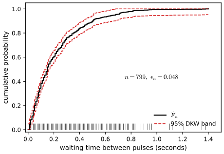
fig_7_1. Download: PDF · SVGExample 7.2 (nerve data). p. 98 The fraction of waiting times between 0.4 and 0.6 seconds is estimated by \(\Fn(0.6)-\Fn(0.4)=0.934-0.841=0.093\) (the book rounds to \(0.93-0.84=0.09\)). This is the proportion of observations in \((0.4,0.6]\), so it is itself an empirical frequency; its standard error is \(\sqrt{0.093\times0.907/799}=0.0103\) and a 95% Normal interval is \((0.073,0.113)\) (Exercise 7.6).
Theorem 7.3 (pointwise properties of \(\Fn\)) p. 98
At any fixed \(x\),
\[ \E\big(\Fn(x)\big)=F(x),\qquad \V\big(\Fn(x)\big)=\frac{F(x)(1-F(x))}{n},\qquad \mse=\frac{F(x)(1-F(x))}{n}\to0,\qquad \Fn(x)\convp F(x). \]Filling the gap 7.2: proof of Theorem 7.3 (Exercise 7.1), and the joint law of \(\Fn\) at several points (Exercises 7.4 and 7.5) p. 98
(a) \(n\Fn(x)\sim\Bin(n,F(x))\); Theorem 7.3 follows, and in fact \(\Fn(x)\convas F(x)\). (b) The central limit theorem holds at each \(x\):
\[ \sqrt n\big(\Fn(x)-F(x)\big)\convd N\big(0,F(x)(1-F(x))\big). \](c) For any \(x,y\),
\[ \Cov\big(\Fn(x),\Fn(y)\big)=\frac{F(\min(x,y))-F(x)F(y)}{n}. \](d) For points \(x_1,\dots,x_k\), the vector \(\sqrt n\big(\Fn(x_j)-F(x_j)\big)_{j}\) converges in distribution to \(N(0,\Sigma)\) with \(\Sigma_{jl}=F(\min(x_j,x_l))-F(x_j)F(x_l)\).
Proof
(a) Let \(Y_i=\I(X_i\le x)\). The \(Y_i\) are iid (functions of independent variables, Chapter 2) and \(\P(Y_i=1)=\P(X_i\le x)=F(x)\), so \(Y_i\sim\Bern(F(x))\) and \(n\Fn(x)=\sum_iY_i\sim\Bin(n,F(x))\). Hence \(\E\Fn(x)=F(x)\) and \(\V\Fn(x)=n^{-2}\cdot nF(x)(1-F(x))\). Being unbiased, \(\Fn(x)\) has MSE equal to its variance (Theorem 6.9: \(\mse=\text{bias}^2+\V\)), which is at most \(1/(4n)\to0\). Convergence in quadratic mean implies convergence in probability (Chapter 5, Theorem 5.4), and the strong law (Theorem 5.18) applied to the bounded \(Y_i\) gives almost sure convergence.
(b) The central limit theorem (Theorem 5.8) for the \(Y_i\), with mean \(F(x)\) and variance \(F(x)(1-F(x))\); when \(F(x)\in\{0,1\}\) the variance is 0 and the limit is the point mass at 0.
(c) Write \(Z_i=\I(X_i\le y)\). For \(i\ne l\), \(Y_i\) and \(Z_l\) are independent, so
\[ \Cov\big(\Fn(x),\Fn(y)\big)=\frac{1}{n^2}\sum_{i,l}\Cov(Y_i,Z_l)=\frac{1}{n^2}\sum_i\Cov(Y_i,Z_i)=\frac1n\Big(\E(Y_1Z_1)-F(x)F(y)\Big), \]and \(Y_1Z_1=\I(X_1\le x,\,X_1\le y)\)
(d) The vectors \(\big(\I(X_i\le x_1),\dots,\I(X_i\le x_k)\big)\) are iid with mean \((F(x_j))_j\) and covariance matrix \(\Sigma\) by the computation in (c); apply the multivariate central limit theorem (Theorem 5.12). ∎
The Brownian bridge. With \(u=F(x)\) and \(v=F(y)\), \(\Sigma\) has entries \(\min(u,v)-uv\): the covariance of the Brownian bridge \(B(u)\), \(0\le u\le1\), a Gaussian process tied to 0 at both ends. Part (d) says that the finite-dimensional laws of the empirical process \(\sqrt n(\Fn-F)\) converge to those of \(B(F(x))\); Donsker's theorem (Donsker, 1952) upgrades this to convergence of the whole process, and that is where Kolmogorov's limit law in Filling the gap 7.5 comes from: \(\sqrt nD_n\convd\sup_u|B(u)|\) for continuous \(F\). Figure 7.S1 confirms (a) to (c) by simulation.
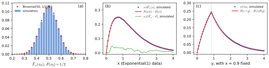
fig_7_s1. Download: PDF · SVGTheorem 7.3 is a statement at one \(x\) at a time. The next theorem is about all \(x\) at once, which is much stronger: there are uncountably many \(x\), and for each sample some of them are always estimated badly. The book states it without proof.
Theorem 7.4 (the Glivenko–Cantelli theorem) p. 98
Let \(X_1,\dots,X_n\sim F\). Then
\[ D_n=\sup_x\big|\Fn(x)-F(x)\big|\convp0, \]and, more precisely (the book's footnote), \(D_n\convas0\).
Filling the gap 7.3: proof of the Glivenko–Cantelli theorem p. 98
For every cdf \(F\) (continuous or not), \(D_n\) is a random variable and \(D_n\to0\) almost surely.
Proof
Measurability. A supremum over uncountably many \(x\) need not be measurable, but here it is a supremum over the rationals: both \(\Fn\) and \(F\) are right-continuous, so for any \(x\) and rationals \(q\downarrow x\), \(|\Fn(q)-F(q)|\to|\Fn(x)-F(x)|\). Hence \(D_n=\sup_{q\in\mathbb Q}|\Fn(q)-F(q)|\), a countable supremum of random variables.
A finite grid. Fix an integer \(k\ge2\) and let \(t_j=F^{-1}(j/k)=\inf\{x:F(x)\ge j/k\}\) for \(j=1,\dots,k-1\), with \(t_0=-\infty\) and \(t_k=+\infty\). Because \(F\) is right-continuous the infimum is attained, so \(F(t_j)\ge j/k\), and every \(x<t_j\) has \(F(x)<j/k\), so the left limit satisfies \(F(t_j-)\le j/k\). For \(x\in[t_{j-1},t_j)\), monotonicity of \(\Fn\) and \(F\) gives
\[ \begin{aligned} \Fn(x)-F(x)&\le\Fn(t_j-)-F(t_{j-1})\\ &=\big[\Fn(t_j-)-F(t_j-)\big]+\big[F(t_j-)-F(t_{j-1})\big]\le\big[\Fn(t_j-)-F(t_j-)\big]+\tfrac1k,\\ \Fn(x)-F(x)&\ge\Fn(t_{j-1})-F(t_j-)\\ &=\big[\Fn(t_{j-1})-F(t_{j-1})\big]-\big[F(t_j-)-F(t_{j-1})\big]\ge\big[\Fn(t_{j-1})-F(t_{j-1})\big]-\tfrac1k, \end{aligned} \]using \(F(t_j-)-F(t_{j-1})\le j/k-(j-1)/k\) (with \(F(-\infty)=\Fn(-\infty)=0\) and the left limits at \(+\infty\) equal to 1). The intervals \([t_{j-1},t_j)\) cover \(\R\), so
\[ D_n\le M_{n,k}+\frac1k,\qquad M_{n,k}=\max_{1\le j\le k-1}\max\Big\{\big|\Fn(t_j)-F(t_j)\big|,\ \big|\Fn(t_j-)-F(t_j-)\big|\Big\}. \]The strong law at finitely many points. \(\Fn(t_j)\) is the average of the iid indicators \(\I(X_i\le t_j)\) with mean \(F(t_j)\), and \(\Fn(t_j-)\) the average of \(\I(X_i<t_j)\) with mean \(F(t_j-)\). By the strong law (Theorem 5.18) each of these \(2(k-1)\) averages converges almost surely; a finite intersection of probability-one events has probability one, so \(M_{n,k}\to0\) almost surely and \(\limsup_nD_n\le1/k\) almost surely.
All grids at once. Let \(A_k=\{\limsup_nD_n\le1/k\}\). Each \(A_k\) has probability one, hence so does the countable intersection \(\bigcap_{k\ge2}A_k=\{\limsup_nD_n=0\}\). So \(D_n\to0\) almost surely, which implies \(D_n\convp0\) (Theorem 5.17). ∎
Two remarks. The left limits matter only when \(F\) has atoms; for continuous \(F\) the grid points \(t_j\) alone suffice. And the argument uses nothing about \(F\) beyond monotonicity: the price of "every \(F\)" is that the proof gives no rate. The rate comes from the DKW inequality below; the exact order of the largest fluctuations along a path is \(\sqrt{\log\log n/(2n)}\) (Chung, 1949), the dotted curve in the Glivenko–Cantelli demo.
See also (companion courses): the same theorem with a shorter proof in Filling the gap 3.7 of Statistical Methods for Modern Biology; uniform laws of large numbers over classes of sets of finite VC dimension, Section 7.9 of Statistical Learning: Theory and Methods.
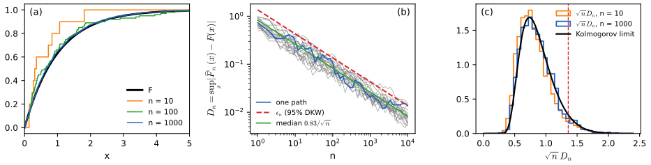
fig_7_s2. Download: PDF · SVGFilling the gap 7.4: every \(F\) reduces to the uniform case pp. 98–99
Let \(U_1,\dots,U_n\) be iid \(\Unif(0,1)\), \(G_n\) their empirical cdf and \(D_n^U=\sup_{0\le u\le1}|G_n(u)-u|\). Put \(X_i=F^{-1}(U_i)\), with \(F^{-1}(u)=\inf\{x:F(x)\ge u\}\). Then (a) the \(X_i\) are iid with cdf \(F\); (b) \(\Fn(x)=G_n(F(x))\) for every \(x\); (c) \(D_n\le D_n^U\), with equality when \(F\) is continuous. Consequently the law of \(D_n\) is the same for every continuous \(F\) (Normal, Cauchy, anything), and for any \(F\) it is stochastically smaller than in the continuous case: \(\P(D_n>\eps)\le\P(D_n^U>\eps)\) for all \(\eps\).
Proof
The switching identity. For \(u\in(0,1)\) and real \(x\), \(F^{-1}(u)\le x\iff u\le F(x)\). Indeed, if \(u\le F(x)\) then \(x\) belongs to the set whose infimum is \(F^{-1}(u)\); conversely the infimum is attained (right-continuity), so \(F(F^{-1}(u))\ge u\), and if \(F^{-1}(u)\le x\) then \(F(x)\ge F(F^{-1}(u))\ge u\).
(a) \(\P(X_i\le x)=\P(U_i\le F(x))=F(x)\); independence is preserved by applying a function to each \(U_i\). This is the inverse-cdf sampling of Chapter 2 (Result 2.4). (b) By the switching identity,
\[ \Fn(x)=\frac1n\#\{i:F^{-1}(U_i)\le x\}=\frac1n\#\{i:U_i\le F(x)\}=G_n(F(x)). \](c) By (b), \(D_n=\sup_x|G_n(F(x))-F(x)|\), a supremum of \(|G_n(u)-u|\) over the range \(\{F(x):x\in\R\}\subset[0,1]\); this is at most the supremum over all of \([0,1]\). If \(F\) is continuous its range contains \((0,1)\) by the intermediate value theorem, and \(|G_n(u)-u|\) at \(u=0\) and \(u=1\) is 0 almost surely, so the two suprema coincide. Since (a) shows that the constructed \(X_i\) are a valid sample from \(F\), the law of \(D_n\) is that of a quantity bounded by \(D_n^U\). ∎
Two consequences used below. First, a bound on \(\P(D_n^U>\eps)\) is a bound for every \(F\) at once: it suffices to prove the DKW inequality for uniforms. Second, for discrete \(F\) the band of Definition 7.A is conservative, because \(D_n\) only looks at the \(u\) values \(F\) actually takes. In the DKW demo the Normal, Cauchy and Exponential samples are built from the same uniforms and the band covers in exactly the same samples (presets 2 and 3); for Poisson(3) data the 95% band covers 992 times in 1000 (preset 4).
Computing \(D_n\). Between order statistics \(G_n\) is constant and \(u\) increases, so the supremum is attained at the jumps:
\[ D_n^U=\max_{1\le i\le n}\max\Big\{\frac in-U_{(i)},\ U_{(i)}-\frac{i-1}n\Big\}. \]For continuous \(F\) this is \(D_n\) with \(U_{(i)}=F(X_{(i)})\); for discrete \(F\) both \(\Fn\) and \(F\) are constant between support points, so \(D_n\) is a maximum over the support. The code uses these two formulas (sup_dist_uniform, sup_dist_discrete_u).
p. 99 The next result quantifies Glivenko–Cantelli with an explicit, distribution-free tail bound. It is the key to a confidence band.
Theorem 7.5 (the Dvoretzky–Kiefer–Wolfowitz (DKW) inequality) p. 99, (7.2)
Let \(X_1,\dots,X_n\sim F\). Then, for any \(\eps>0\),
\[ \P\Big(\sup_x\big|F(x)-\Fn(x)\big|>\eps\Big)\le2e^{-2n\eps^2}. \tag{7.2} \]Compare Hoeffding's inequality for a single proportion (Chapter 4, Theorem 4.5): at one fixed \(x\), \(\P(|\Fn(x)-F(x)|>\eps)\le2e^{-2n\eps^2}\). The DKW inequality says that the supremum over all \(x\) satisfies the same bound, with the same constant: estimating the whole cdf is, in this sense, no harder than estimating one probability.
Filling the gap 7.5: a DKW inequality with a complete proof, the constant 2, and Kolmogorov's limit p. 99
(a) An elementary version. For every \(F\), every \(n\), every \(\eps>0\) and every integer \(k>1/\eps\),
\[ \P(D_n>\eps)\le2(k-1)\,e^{-2n(\eps-1/k)^2}. \](b) The constant 2. Dvoretzky, Kiefer and Wolfowitz (1956) proved (7.2) with an unspecified constant \(C\) in place of 2; Massart (1990) proved that \(C=2\) works for all \(n\) and \(\eps\). (c) It cannot be improved. For continuous \(F\) and every \(t>0\),
\[ \P\big(\sqrt nD_n>t\big)\to2\sum_{k=1}^\infty(-1)^{k-1}e^{-2k^2t^2}\quad(n\to\infty), \]Kolmogorov's (1933) limit law, and the right side is at most \(2e^{-2t^2}\) but equals \(2e^{-2t^2}(1+o(1))\) as \(t\to\infty\): no constant smaller than 2 is valid for all \(n\) and \(\eps\).
Proof of (a), and what is known about (b) and (c)
(a) By Filling the gap 7.4 it suffices to bound \(\P(D_n^U>\eps)\) for uniform data. Let \(t_j=j/k\), \(j=0,\dots,k\). For \(u\in[t_{j-1},t_j]\), monotonicity gives
\[ \begin{aligned} G_n(u)-u&\le G_n(t_j)-t_{j-1}=\big(G_n(t_j)-t_j\big)+\tfrac1k,\\ G_n(u)-u&\ge G_n(t_{j-1})-t_j=\big(G_n(t_{j-1})-t_{j-1}\big)-\tfrac1k. \end{aligned} \]Since \(G_n(0)=0\) and \(G_n(1)=1\) almost surely, \(D_n^U\le\max_{1\le j\le k-1}|G_n(t_j)-t_j|+1/k\). So \(D_n^U>\eps\) forces \(|G_n(t_j)-t_j|>\eps-1/k>0\) for some \(j\le k-1\); each \(G_n(t_j)\) is a proportion of \(n\) Bernoulli(\(t_j\)) trials, so by Hoeffding's inequality (Theorem 4.5) and a union bound over the \(k-1\) points,
\[ \P(D_n^U>\eps)\le\sum_{j=1}^{k-1}\P\big(|G_n(t_j)-t_j|>\eps-\tfrac1k\big)\le2(k-1)e^{-2n(\eps-1/k)^2}. \]Optimising over \(k\) (roughly \(k\approx\sqrt n\)) gives a band of half-width of order \(\sqrt{\log n/n}\) rather than \(1/\sqrt n\). For \(n=799\) and \(\alpha=0.05\) the smallest \(\eps\) for which the bound reaches 0.05 is 0.080, against \(\eps_n=0.048\) from (7.2); for \(n=100\), 0.213 against 0.136. The elementary argument loses a logarithm because it ignores that the \(k-1\) proportions are strongly dependent; recovering the sharp constant needs the finer structure of the uniform empirical process. ∎
(b) Massart's proof (1990) is a delicate analysis of the uniform empirical process, beyond this course; the bound holds as stated whenever \(2e^{-2n\eps^2}\le1\), and is trivially true otherwise.
(c) The limit is the law of \(\sup_u|B(u)|\) for a Brownian bridge (Filling the gap 7.2); its derivation (Kolmogorov, 1933; Donsker, 1952) is beyond this course, but the comparison with the bound is elementary. The terms \(e^{-2k^2t^2}\) decrease in \(k\), so the alternating series lies between its first partial sums: \(2e^{-2t^2}-2e^{-8t^2}\le\) limit \(\le2e^{-2t^2}\). The ratio of the lower bound to \(2e^{-2t^2}\) is \(1-e^{-6t^2}\to1\). If (7.2) held with \(C<2\), letting \(n\to\infty\) at \(\eps=t/\sqrt n\) would give \(2e^{-2t^2}-2e^{-8t^2}\le Ce^{-2t^2}\), false for large \(t\).
Numbers. The exact law of \(D_n\) for continuous \(F\) can be computed (Figure 7.S3). With \(\eps_n=\sqrt{\log(2/\alpha)/(2n)}\) and \(\alpha=0.05\), the exact coverage \(\P(D_n\le\eps_n)\) is 0.9657 for \(n=10\), 0.9547 for \(n=100\), 0.9516 for \(n=799\); its limit is \(1-2\sum_k(-1)^{k-1}(\alpha/2)^{k^2}=0.9500008\). So the DKW band is slightly conservative for small \(n\) and essentially exact for large \(n\). The limit law of \(\sqrt nD_n\) has median 0.828 and mean \(\sqrt{\pi/2}\,\log2=0.869\).
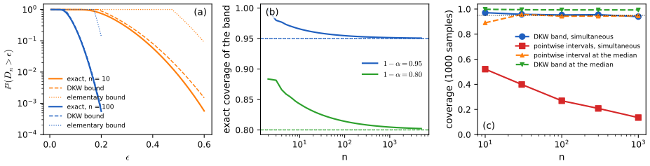
fig_7_s3. Download: PDF · SVGDefinition 7.A (a nonparametric \(1-\alpha\) confidence band for \(F\)) p. 99, (7.3)
Define
\[ L(x)=\max\{\Fn(x)-\eps_n,\,0\},\qquad U(x)=\min\{\Fn(x)+\eps_n,\,1\},\qquad \eps_n=\sqrt{\frac{1}{2n}\log\Big(\frac2\alpha\Big)}. \]It follows from (7.2) that for any \(F\),
\[ \P\big(L(x)\le F(x)\le U(x)\ \text{for all }x\big)\ge1-\alpha. \tag{7.3} \]Filling the gap 7.6: why (7.3) follows, what the band buys, and what it costs p. 99
(a) (7.3) holds for every \(F\) and every \(n\). (b) On the same event of probability at least \(1-\alpha\), every quantity that is monotone in \(F\) is trapped at once; for instance, simultaneously for all \(a<b\),
\[ \max\{L(b)-U(a),0\}\le F(b)-F(a)\le\min\{U(b)-L(a),1\}. \](c) The half-width is \(\eps_n\); a half-width \(\eps\) needs \(n\ge\log(2/\alpha)/(2\eps^2)\). (d) The pointwise Normal intervals \(\Fn(x)\pm z_{\alpha/2}\sqrt{\Fn(x)(1-\Fn(x))/n}\) are narrower (at most \(z_{\alpha/2}/(2\sqrt n)\)) and each covers \(F(x)\) with probability close to \(1-\alpha\), but taken together they do not form a \(1-\alpha\) band.
Proof and numbers
(a) Let \(A=\{D_n\le\eps_n\}\). By (7.2), \(\P(A^c)\le2e^{-2n\eps_n^2}=2e^{-\log(2/\alpha)}=\alpha\). On \(A\), \(\Fn(x)-\eps_n\le F(x)\le\Fn(x)+\eps_n\) for every \(x\), and since \(0\le F(x)\le1\) the clipped bounds hold too: \(L(x)\le F(x)\le U(x)\). Hence the event in (7.3) contains \(A\) and has probability at least \(1-\alpha\).
(b) On the event of (7.3), \(F(b)\le U(b)\) and \(F(a)\ge L(a)\), so \(F(b)-F(a)\le U(b)-L(a)\); the lower bound is symmetric, and \(F(b)-F(a)\in[0,1]\). Because the event does not depend on \(a,b\), the statement is simultaneous. For the nerve data, \(F(0.6)-F(0.4)\) lies in \((0,0.189)\): honest about all intervals at once, but much wider than the interval \((0.073,0.113)\) for this one pair (Exercise 7.6).
(c) Solve \(\sqrt{\log(2/\alpha)/(2n)}\le\eps\). For \(\alpha=0.05\) and \(\eps=0.05\), \(n\ge738\); for \(\eps=0.01\), \(n\ge18\,445\). The nerve data have \(n=799\) and \(\eps_n=0.048\), Example 7.6.
(d) Each pointwise interval is the Wald interval for a proportion, with coverage tending to \(1-\alpha\) (Chapter 6, Theorem 6.16), and its half-width is largest when \(\Fn=1/2\). But the event that all of them cover is an intersection over infinitely many \(x\), whose probability is much smaller. In 1000 Normal samples of size 100 (the stream of the DKW demo), the band contains \(F\) in 953 samples (exact probability 0.9547), while the pointwise intervals contain \(F\) at every \(x\in[X_{(1)},X_{(n)})\) in only 269; at \(n=1000\) in about 14%. At the single point \(x=\) median of \(F\), the exact coverage of the pointwise interval is 0.943 and that of the band 0.993 (\(n=100\)). The ratio of the two half-widths at the median, \(\eps_n/(z_{\alpha/2}/(2\sqrt n))\)
Example 7.6. p. 99 For the nerve data, \(n=799\) and \(\alpha=0.05\) give \(\eps_n=\sqrt{\log(40)/1598}=0.048\), the band of Figure 7.1.
See also (companion course): the DKW band on gene expression data and a coverage experiment for a two-component mixture, in the ECDF and QQ-plot demo of Statistical Methods for Modern Biology.
7.2 Statistical Functionals
p. 99 A statistical functional \(T(F)\) is any function of \(F\) (Chapter 6, Definition 6.B): the mean \(\mu=\int x\,\d F(x)\), the variance \(\sigma^2=\int(x-\mu)^2\,\d F(x)\), the median \(m=F^{-1}(1/2)\). Since \(\Fn\) estimates \(F\) well, a natural estimate of \(T(F)\) is \(T(\Fn)\).
Definition 7.7 (plug-in estimator) p. 99
The plug-in estimator of \(\th=T(F)\) is \(\hth=T(\Fn)\): plug in \(\Fn\) for the unknown \(F\).
Definition 7.8 (linear functional) p. 99
If \(T(F)=\int r(x)\,\d F(x)\) for some function \(r\), then \(T\) is a linear functional.
p. 100 The name comes from \(T(aF+bG)=aT(F)+bT(G)\): the integral is linear in the distribution. (For \(aF+bG\) to be a cdf one needs \(a,b\ge0\) and \(a+b=1\); then \(aF+bG\) is the mixture that draws from \(F\) with probability \(a\), and the identity is the law of total expectation.)
Theorem 7.9 (plug-in for a linear functional) p. 100, (7.4)
The plug-in estimator for the linear functional \(T(F)=\int r(x)\,\d F(x)\) is
\[ T(\Fn)=\int r(x)\,\d\Fn(x)=\frac1n\sum_{i=1}^nr(X_i). \tag{7.4} \]Filling the gap 7.7: linear plug-in estimators are unbiased, consistent and asymptotically Normal p. 100, (7.5)–(7.6)
Suppose \(\E\,r(X)^2<\infty\) and put \(\sigma_r^2=\V(r(X))\). Then (a) \(T(\Fn)\) is unbiased with \(\se=\sigma_r/\sqrt n\); (b) \(T(\Fn)\to T(F)\) almost surely; (c) \(\sqrt n(T(\Fn)-T(F))\convd N(0,\sigma_r^2)\), which is (7.5); (d) with \(\widehat\sigma_r^2=n^{-1}\sum_i(r(X_i)-T(\Fn))^2\), the Normal-based interval (7.6), \(T(\Fn)\pm z_{\alpha/2}\widehat\sigma_r/\sqrt n\), has coverage tending to \(1-\alpha\) whenever \(\sigma_r>0\).
Proof
Equation (7.4) is Filling the gap 7.1(c). The \(r(X_i)\) are iid with mean \(T(F)\) and variance \(\sigma_r^2\), so (a) is linearity of expectation and the variance of an average of independent terms; (b) is the strong law; (c) is the central limit theorem. (d) \(\widehat\sigma_r^2=n^{-1}\sum_ir(X_i)^2-T(\Fn)^2\) converges almost surely to \(\E r(X)^2-T(F)^2=\sigma_r^2\) by the strong law, so \(\widehat\sigma_r/\sigma_r\convp1\), and by Slutsky's theorem (Chapter 5, Theorem 5.10) \(\sqrt n(T(\Fn)-T(F))/\widehat\sigma_r\convd N(0,1)\). The coverage is \(\P\big(|\sqrt n(T(\Fn)-T(F))/\widehat\sigma_r|\le z_{\alpha/2}\big)\)
Two cautions. The guarantee is pointwise in \(F\), not uniform (Chapter 6, Definition 6.F): for heavily skewed \(F\) the \(n\) needed can be large. And without \(\E r(X)^2<\infty\) there is no standard error at all: for Cauchy data the sample mean does not even converge (Chapter 6, Filling the gap 6.6), although the DKW band, which needs no moments, works perfectly.
p. 100 In many cases, as for linear functionals,
\[ T(\Fn)\approx N\big(T(F),\se^2\big), \tag{7.5} \]and an approximate \(1-\alpha\) confidence interval for \(T(F)\), the Normal-based interval, is
\[ T(\Fn)\pm z_{\alpha/2}\,\hse. \tag{7.6} \]For 95% intervals \(z_{0.025}=1.96\approx2\), and the interval is \(T(\Fn)\pm2\hse\). The book postpones a general way of finding \(\hse\) to the bootstrap of Chapter 8; Filling the gap 7.12 gives one now.
Example 7.10 (the mean). p. 100 With \(r(x)=x\), \(\widehat\mu=\Xb\), \(\se=\sqrt{\V(\Xb)}=\sigma/\sqrt n\), estimated by \(\widehat\sigma/\sqrt n\), and the Normal-based interval is \(\Xb\pm z_{\alpha/2}\hse\). For the nerve data, \(\Xb=0.2186\) seconds with \(\hse=0.0074\).
Example 7.11 (the variance). pp. 100–101 With \(\sigma^2=T(F)=\int x^2\,\d F(x)-(\int x\,\d F(x))^2\), the plug-in estimator is
\[ \widehat\sigma^2=\int x^2\,\d\Fn(x)-\Big(\int x\,\d\Fn(x)\Big)^2=\frac1n\sum_{i=1}^nX_i^2-\Big(\frac1n\sum_{i=1}^nX_i\Big)^2=\frac1n\sum_{i=1}^n(X_i-\Xb)^2. \]Another reasonable estimator is the sample variance \(S_n^2=\frac{1}{n-1}\sum_i(X_i-\Xb)^2\); the book notes that there is little difference in practice. With this, the estimated standard error of the mean in Example 7.10 is \(\widehat\sigma/\sqrt n\). The variance is not a linear functional (it is not linear in \(F\)), but it is a smooth function of two linear ones.
Filling the gap 7.8: the plug-in variance, its bias and its standard error pp. 100–101
Let \(\mu_k=\E(X-\mu)^k\) be the central moments and suppose \(\mu_4<\infty\). Then (a) \(\E\widehat\sigma^2=\frac{n-1}{n}\sigma^2\) and \(\E S_n^2=\sigma^2\); (b) \(\V(S_n^2)=\frac1n\big(\mu_4-\frac{n-3}{n-1}\sigma^4\big)\); (c) \(\sqrt n(\widehat\sigma^2-\sigma^2)\convd N(0,\mu_4-\sigma^4)\), and the same holds for \(S_n^2\), so the two estimators are asymptotically equivalent; (d) \(\hse(\widehat\sigma^2)=\sqrt{(\widehat\mu_4-\widehat\sigma^4)/n}\) with \(\widehat\mu_4=n^{-1}\sum_i(X_i-\Xb)^4\) is consistent in the sense \(\sqrt n\,\hse\convp\sqrt{\mu_4-\sigma^4}\).
Proof
(a) is Chapter 3 (Result 3.7): \(\E\sum_i(X_i-\Xb)^2=(n-1)\sigma^2\). (b) Without loss of generality \(\mu=0\). Expand \(\sum_i(X_i-\Xb)^2=\sum_iX_i^2-n\Xb^2\) and compute the second moment term by term using independence: the only nonzero expectations of products of four \(X\)'s are \(\E X_i^4=\mu_4\) and \(\E X_i^2X_j^2=\sigma^4\) (\(i\ne j\)). Collecting terms gives
\[ \E\Big(\sum_i(X_i-\Xb)^2\Big)^2=\frac{(n-1)^2}{n}\mu_4+\frac{(n-1)(n^2-2n+3)}{n}\sigma^4, \]and subtracting \(((n-1)\sigma^2)^2\) and dividing by \((n-1)^2\) gives (b). (c) \(\widehat\sigma^2=a(\overline{X^2},\Xb)\) with \(a(t_2,t_1)=t_2-t_1^2\). The pair of averages is asymptotically Normal by the multivariate central limit theorem, and the multivariate delta method (Chapter 5, Theorem 5.15) with gradient \((1,-2\mu)\) gives the limit variance \(\V(X^2-2\mu X)=\V((X-\mu)^2)=\mu_4-\sigma^4\). Since \(S_n^2-\widehat\sigma^2=\widehat\sigma^2/(n-1)\), we have \(\sqrt n(S_n^2-\widehat\sigma^2)\convp0\) and Slutsky's theorem transfers the limit. (d) \(\widehat\mu_4\) and \(\widehat\sigma^2\) are continuous functions of the first four sample moments, which converge almost surely. ∎
For Normal data \(\mu_4=3\sigma^4\) and \(\se(\widehat\sigma^2)\approx\sigma^2\sqrt{2/n}\); for Exponential data \(\mu_4=9\sigma^4\) and the standard error is twice as large. The fourth moment is itself hard to estimate, so \(\hse\) tends to be too small for skewed data: with Exponential samples of size 100 the interval (7.6) for \(\sigma^2\) covers only 85% of the time (Figure 7.S4).
See also: the bias of \(\widehat\sigma^2\) in this course's sample variance demo (Chapter 3); in the companion course Bayesian and Probabilistic Machine Learning, the bias of the maximum likelihood variance, Result 1.8.
Example 7.12 (the skewness). p. 101 The skewness measures the lack of symmetry of a distribution:
\[ \kappa=\frac{\E(X-\mu)^3}{\sigma^3}=\frac{\int(x-\mu)^3\,\d F(x)}{\big(\int(x-\mu)^2\,\d F(x)\big)^{3/2}},\qquad \widehat\kappa=\frac{\frac1n\sum_i(X_i-\widehat\mu)^3}{\widehat\sigma^3}. \]For the nerve data \(\widehat\kappa=1.76\): the waiting times are strongly skewed to the right, as Figure 7.1 shows (an Exponential distribution has \(\kappa=2\)).
Filling the gap 7.9: the standard error of the skewness p. 101
If \(\E X^6<\infty\), then \(\widehat\kappa\convas\kappa\) and \(\sqrt n(\widehat\kappa-\kappa)\convd N(0,\tau^2)\), with
\[ \tau^2=\E\Big[\big(Z^3-\tfrac32\kappa Z^2-3Z+\tfrac12\kappa\big)^2\Big],\qquad Z=\frac{X-\mu}\sigma. \]For Normal data \(\tau^2=6\); for Exponential data \(\tau^2=72\).
Proof
\(\widehat\kappa=a(\overline X,\overline{X^2},\overline{X^3})\) for the smooth function
\[ a(t_1,t_2,t_3)=\frac{t_3-3t_1t_2+2t_1^3}{(t_2-t_1^2)^{3/2}},\qquad t_2>t_1^2. \]Consistency follows from the strong law and continuity of \(a\). The vector of the three averages is asymptotically Normal when \(\E X^6<\infty\) (the covariance matrix involves moments up to order 6), and the multivariate delta method gives a Normal limit with variance \(\V(L(X))\), where \(L(x)=\sum_j\partial_ja\,(x^j-\E X^j)\). The cleanest way to compute \(L\) is the chain rule of Filling the gap 7.12: with \(m_k=\int(x-\mu)^k\,\d F\), \(\kappa=m_3/m_2^{3/2}\), and the influence functions \(L_{m_2}(x)=(x-\mu)^2-m_2\) and \(L_{m_3}(x)=(x-\mu)^3-m_3-3m_2(x-\mu)\) give
\[ L(x)=\frac{L_{m_3}(x)}{\sigma^3}-\frac32\frac{m_3}{\sigma^5}L_{m_2}(x)=Z^3-\kappa-3Z-\tfrac32\kappa(Z^2-1)=Z^3-\tfrac32\kappa Z^2-3Z+\tfrac12\kappa. \]\(\E L=0\), so \(\tau^2=\E L^2\). For \(N(0,1)\): \(\kappa=0\), \(\E(Z^3-3Z)^2=15-18+9=6\). For Exponential(1), \(Z=X-1\) has central moments \(\E Z^2,\dots,\E Z^6=1,2,9,44,265\), \(\kappa=2\), and expanding \((Z^3-3Z^2-3Z+1)^2\) term by term gives
\[ \tau^2=265-6\cdot44+(81-54)+(4+36)-6\cdot1-0+9+1=72. \]∎
The cubic influence function is the warning: a single observation far out moves \(\widehat\kappa\) a lot, and \(\tau^2\) involves the sixth moment. For Exponential samples of size 100 the estimates are biased down (mean 1.79 against \(\kappa=2\)), their spread is 0.55 against \(\tau/\sqrt n=0.85\), \(\hse\) averages only 0.32, and the interval (7.6) covers 65% of the time; even at \(n=1000\) it covers 83%. The bootstrap of Chapter 8 does better here because it does not rely on the Normal shape.
Example 7.13 (correlation). pp. 101–102 For a bivariate \(Z=(X,Y)\) with cdf \(F\), the correlation \(\rho=T(F)=\E(X-\mu_X)(Y-\mu_Y)/(\sigma_X\sigma_Y)\) is \(T(F)=a(T_1(F),\dots,T_5(F))\), where
\[ T_1=\int x\,\d F,\quad T_2=\int y\,\d F,\quad T_3=\int xy\,\d F,\quad T_4=\int x^2\,\d F,\quad T_5=\int y^2\,\d F,\qquad a(t_1,\dots,t_5)=\frac{t_3-t_1t_2}{\sqrt{(t_4-t_1^2)(t_5-t_2^2)}}. \]Plugging in \(\Fn\) in each \(T_j\) gives the sample correlation
\[ \widehat\rho=\frac{\sum_i(X_i-\Xb)(Y_i-\overline Y_n)}{\sqrt{\sum_i(X_i-\Xb)^2}\sqrt{\sum_i(Y_i-\overline Y_n)^2}}. \]For the 272 Old Faithful eruptions, the correlation between eruption duration and waiting time is \(\widehat\rho=0.901\).
Filling the gap 7.10: the standard error of the sample correlation p. 102
If \(\E X^4,\E Y^4<\infty\) and \(\sigma_X,\sigma_Y>0\), then \(\widehat\rho\convas\rho\) and \(\sqrt n(\widehat\rho-\rho)\convd N(0,\tau^2)\) with
\[ \tau^2=\E\Big[\big(\tilde X\tilde Y-\tfrac12\rho(\tilde X^2+\tilde Y^2)\big)^2\Big],\qquad \tilde X=\frac{X-\mu_X}{\sigma_X},\ \tilde Y=\frac{Y-\mu_Y}{\sigma_Y}. \]For bivariate Normal data, \(\tau^2=(1-\rho^2)^2\).
Proof
Consistency: the five averages converge almost surely and \(a\) is continuous where the denominator is positive. Asymptotic normality: the five averages \((\overline X,\overline Y,\overline{XY},\overline{X^2},\overline{Y^2})\) are jointly asymptotically Normal (fourth moments are needed for their covariances) and \(a\) is differentiable, so the multivariate delta method applies. Its variance is \(\V(L(X,Y))\) for the influence function, which the chain rule (Filling the gap 7.12) computes most easily after standardising (\(\rho\) is invariant under \(x\mapsto(x-\mu_X)/\sigma_X\), \(y\mapsto(y-\mu_Y)/\sigma_Y\), so take \(\mu=0\), \(\sigma=1\)): perturbing \(F\) towards a point mass at \((x,y)\) changes the covariance by \(xy-\rho\) and each variance by \(x^2-1\) and \(y^2-1\), so
\[ L(x,y)=(xy-\rho)-\tfrac12\rho\,(x^2-1)-\tfrac12\rho\,(y^2-1)=xy-\tfrac12\rho(x^2+y^2). \]For the bivariate Normal, write \(Y=\rho X+\sqrt{1-\rho^2}\,W\) with \(W\) independent of \(X\) and use \(\E X^4=3\): a direct expansion gives \(\E L^2=(1-\rho^2)^2\). ∎
The variance shrinks as \(|\rho|\to1\), but the Normal approximation is poor there because \(\widehat\rho\le1\): for Old Faithful pairs resampled \(n=50\) at a time, the interval covers 91.7%. Fisher's transformation \(\tfrac12\log\frac{1+\widehat\rho}{1-\widehat\rho}\), whose asymptotic variance under normality is \(1/n\) for every \(\rho\) by the delta method, is the usual remedy (Fisher, 1915).
Example 7.14 (quantiles). p. 102 Let \(F\) be strictly increasing with density \(f\). For \(0<p<1\) the \(p\)th quantile is \(T(F)=F^{-1}(p)\). Because \(\Fn\) is a step function and not invertible, the book defines
\[ \Fn^{-1}(p)=\inf\{x:\Fn(x)\ge p\}, \]the \(p\)th sample quantile. By Filling the gap 7.1(d), \(\Fn^{-1}(p)=X_{(\lceil np\rceil)}\). For the nerve data the sample median is \(X_{(400)}=0.15\) and the 0.9 quantile \(X_{(720)}=0.51\).
Filling the gap 7.11: sample quantiles are consistent and asymptotically Normal p. 102
Let \(\xi_p=F^{-1}(p)\) and \(\widehat\xi_p=\Fn^{-1}(p)\). (a) If \(F(\xi_p-\delta)<p<F(\xi_p+\delta)\) for every \(\delta>0\) (true when \(F\) is strictly increasing near \(\xi_p\)), then \(\widehat\xi_p\convas\xi_p\). (b) If \(F\) is differentiable at \(\xi_p\) with \(f(\xi_p)>0\), then
\[ \sqrt n\big(\widehat\xi_p-\xi_p\big)\convd N\Big(0,\ \frac{p(1-p)}{f(\xi_p)^2}\Big). \]For the median of Normal data the asymptotic variance is \(\pi\sigma^2/2\), about 1.57 times that of the mean.
Proof
Switching. For any \(x\), \(\widehat\xi_p\le x\iff\Fn(x)\ge p\) (Filling the gap 7.4, applied to the cdf \(\Fn\)). So statements about the sample quantile become statements about a binomial proportion.
(a) Fix \(\delta>0\). By the strong law, \(\Fn(\xi_p+\delta)\to F(\xi_p+\delta)>p\) and \(\Fn(\xi_p-\delta)\to F(\xi_p-\delta)<p\) almost surely. Hence, almost surely, for all large \(n\): \(\Fn(\xi_p+\delta)\ge p\), so \(\widehat\xi_p\le\xi_p+\delta\); and \(\Fn(\xi_p-\delta)<p\), so \(\widehat\xi_p>\xi_p-\delta\). Intersect over \(\delta=1/m\), \(m=1,2,\dots\).
(b) Fix \(t\) and let \(x_n=\xi_p+t/\sqrt n\), \(p_n=F(x_n)\). Differentiability gives \(p_n=p+f(\xi_p)t/\sqrt n+o(1/\sqrt n)\), and continuity at \(\xi_p\) gives \(F(\xi_p)=p\). By switching,
\[ \P\big(\sqrt n(\widehat\xi_p-\xi_p)\le t\big)=\P\big(\Fn(x_n)\ge p\big)=\P\bigg(\frac{\sqrt n(\Fn(x_n)-p_n)}{\sqrt{p_n(1-p_n)}}\ge c_n\bigg),\quad c_n=\frac{\sqrt n(p-p_n)}{\sqrt{p_n(1-p_n)}}\to-\frac{f(\xi_p)\,t}{\sqrt{p(1-p)}}. \]Here \(n\Fn(x_n)\sim\Bin(n,p_n)\) with \(p_n\) changing with \(n\), so the ordinary central limit theorem does not apply directly; the Berry–Esseen inequality (Chapter 5, Theorem 5.11) does. For a standardised \(\Bin(n,q)\), with \(Y\sim\Bern(q)\), the distance to \(\Phi\) is at most
\[ \frac{C\,\E|Y-q|^3}{(q(1-q))^{3/2}\sqrt n}\le\frac{C}{\sqrt{nq(1-q)}}, \]which tends to 0 because \(p_n\to p\in(0,1)\). So the probability above differs from \(1-\Phi(c_n)\) by \(o(1)\), and \(1-\Phi(c_n)\to\Phi\big(f(\xi_p)t/\sqrt{p(1-p)}\big)\), the cdf at \(t\) of \(N(0,p(1-p)/f(\xi_p)^2)\). ∎
Standard error. \(\se(\widehat\xi_p)\approx\sqrt{p(1-p)/n}/f(\xi_p)\) needs the density at the quantile, which is not a plug-in quantity: \(\Fn\) has no density. In practice \(f(\widehat\xi_p)\) is estimated, for instance by a kernel density estimate (Chapter 20); the code and the demo use a Gaussian kernel with the normal-reference bandwidth (Silverman, 1986). For the nerve data this gives \(\hse=0.0071\) for the median and 0.021 for the 0.9 quantile, but the data have atoms (29 values equal 0.15), so these numbers must be read with care; the bootstrap of Chapter 8 avoids the density altogether. Convention. Chapter 2 of the book defines the quantile function with a strict inequality, \(\inf\{x:F(x)>q\}\) (Definition 2.5 of these notes); for \(\Fn\) and \(p=k/n\) the two conventions give \(X_{(k)}\) and \(X_{(k+1)}\). The limit theorem holds for both, since they differ only when \(np\) is an integer and then by one order statistic (see Notes on the book).
See also (companion course): sample quantiles and the QQ plot in Section 2.6.1 of Statistical Methods for Modern Biology.
p. 102 The book now asks how to get standard errors and intervals for Examples 7.11 to 7.14, and promises parametric formulas (Chapter 9) and the bootstrap (Chapter 8). The boxes above already gave them one by one. They are all instances of one idea, which is worth stating in general because it is exactly what the bootstrap approximates numerically.
Filling the gap 7.12: the influence function and the nonparametric delta method p. 102
Definition. The influence function of \(T\) at \(F\) is the derivative of \(T\) in the direction of a point mass \(\delta_x\):
\[ L_F(x)=\lim_{\eps\downarrow0}\frac{T\big((1-\eps)F+\eps\,\delta_x\big)-T(F)}{\eps}. \]It measures the effect on \(T\) of a small amount of contamination at \(x\) (Hampel, 1974). Examples (Figure 7.S5):
| \(T(F)\) | \(L_F(x)\) | \(\tau^2=\E L_F(X)^2\) |
|---|---|---|
| linear, \(\int r\,\d F\) | \(r(x)-T(F)\) | \(\V(r(X))\) |
| mean \(\mu\) | \(x-\mu\) | \(\sigma^2\) |
| variance \(\sigma^2\) | \((x-\mu)^2-\sigma^2\) | \(\mu_4-\sigma^4\) |
| skewness \(\kappa\) | \(z^3-\frac32\kappa z^2-3z+\frac12\kappa\) | 7.9 |
| correlation \(\rho\) | \(\tilde x\tilde y-\frac12\rho(\tilde x^2+\tilde y^2)\) | 7.10 |
| quantile \(\xi_p\) | \((p-\I(x\le\xi_p))/f(\xi_p)\) | \(p(1-p)/f(\xi_p)^2\) |
The theorem. Let \(T(F)=a(T_1(F),\dots,T_k(F))\) with linear \(T_j(F)=\int r_j\,\d F\), \(\E r_j(X)^2<\infty\), and \(a\) differentiable at \(t=(T_j(F))_j\). Then
\[ L_F(x)=\sum_{j=1}^k\partial_ja(t)\,\big(r_j(x)-T_j(F)\big),\qquad \sqrt n\big(T(\Fn)-T(F)\big)\convd N\big(0,\tau^2\big),\quad \tau^2=\E L_F(X)^2, \]and the plug-in standard error \(\hse=\sqrt{\sum_iL_{\Fn}(X_i)^2}/n\) satisfies \(\sqrt n\,\hse\convp\tau\) if \(a\) is continuously differentiable near \(t\). Consequently the Normal-based interval (7.6) has asymptotic coverage \(1-\alpha\) whenever \(\tau>0\). The same conclusions hold for quantiles under the conditions of Filling the gap 7.11(b), given a consistent estimate of \(f(\xi_p)\).
Proof
The influence functions. For a linear functional, \(T((1-\eps)F+\eps\delta_x)=(1-\eps)T(F)+\eps r(x)\), so the difference quotient is exactly \(r(x)-T(F)\). For \(T=a(T_1,\dots,T_k)\), each \(T_j\) moves along the straight line \(T_j+\eps(r_j(x)-T_j)\), and the chain rule gives the stated sum. The mean and the variance (\(a(t_1,t_2)=t_2-t_1^2\), \(r=(x,x^2)\): \(L=-2\mu(x-\mu)+(x^2-\E X^2)\)
The limit. The vector of averages \(\overline r=(n^{-1}\sum_ir_j(X_i))_j=(T_j(\Fn))_j\) satisfies \(\sqrt n(\overline r-t)\convd N(0,\Sigma)\) with \(\Sigma=\Cov(r(X))\) (Theorem 5.12). The multivariate delta method (Theorem 5.15) gives \(\sqrt n(a(\overline r)-a(t))\convd N(0,\nabla a^\T\Sigma\nabla a)\), and \(\nabla a^\T\Sigma\nabla a=\V\big(\sum_j\partial_ja\,r_j(X)\big)\)
an average of iid mean-zero terms: every smooth plug-in estimator behaves like a sample mean of its influence function.
The standard error. \(L_{\Fn}(x)=\sum_j\partial_ja(\overline r)(r_j(x)-\overline r_j)\), so
\[ n\,\hse^2=\frac1n\sum_iL_{\Fn}(X_i)^2=\nabla a(\overline r)^\T\,\widehat\Sigma\,\nabla a(\overline r), \]with \(\widehat\Sigma\) the plug-in covariance matrix of the \(r(X_i)\). Both \(\overline r\to t\) and \(\widehat\Sigma\to\Sigma\) almost surely (strong law), and \(\nabla a\) is continuous at \(t\), so \(n\,\hse^2\to\tau^2\) almost surely. Slutsky's theorem then gives the coverage, as in Filling the gap 7.7(d). For the quantile, \(\widehat\xi_p\to\xi_p\) by 7.11(a), and a consistent density estimate at a consistent point gives \(\hse\sqrt n\convp\tau\) if \(f\) is continuous at \(\xi_p\). ∎
Beyond smooth functions of means. The general statement, for functionals that are differentiable in a suitable sense (Hadamard differentiability tangentially to continuous functions), is van der Vaart (1998), Theorem 20.8; it covers quantiles, trimmed means and many more. The influence function also explains robustness: the mean, variance and skewness have unbounded \(L_F\) (one wild observation can move them arbitrarily), the median a bounded one. And it explains the bootstrap: resampling from \(\Fn\) estimates the distribution of \(T(\Fn)-T(F)\), whose spread is \(\tau/\sqrt n\) to first order, without computing \(L_F\) at all (Chapter 8).
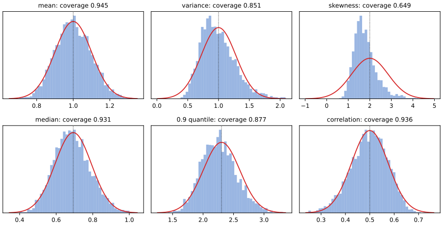
fig_7_s4. Download: PDF · SVG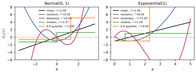
fig_7_s5. Download: PDF · SVGSee also: the delta method of Chapter 5 (Theorem 5.13 and the delta-method demo); the bootstrap standard error in the companion courses: Definition 5.5 of Applied Statistical Learning and Section 7.11 of Statistical Learning: Theory and Methods.
Example 7.15 (plasma cholesterol). pp. 102–103 Plasma cholesterol (mg/dl) was measured on 371 patients with chest pain (Scott et al., 1978): 51 with no evidence of heart disease and 320 with narrowing of the arteries. The book's Figure 7.2 shows the two histograms; the data are not distributed with the book, so the figure is not reproduced here, but every number of the example can be re-derived from the summaries it quotes. Treat the groups as samples from \(F_1\) and \(F_2\) with means \(\mu_1,\mu_2\). The plug-in estimates are \(\widehat\mu_1=195.27\) and \(\widehat\mu_2=216.19\), with \(\hse(\widehat\mu_j)=\widehat\sigma_j/\sqrt{n_j}\) equal to 5.0 and 2.4 (so \(\widehat\sigma_1\approx35.7\) and \(\widehat\sigma_2\approx42.9\)); the intervals \(\widehat\mu_j\pm2\hse\) are \((185,205)\) and \((211,221)\). For \(\th=\mu_2-\mu_1\), \(\hth=20.92\) and
\[ \hse(\hth)=\sqrt{\hse(\widehat\mu_1)^2+\hse(\widehat\mu_2)^2}=\sqrt{5.0^2+2.4^2}=5.55, \]so the approximate 95% interval is \(20.92\pm2\times5.55=(9.8,32.0)\): cholesterol is higher, on average, in the group with narrowed arteries. As the book stresses, this is an association; whether cholesterol causes the disease is a question for Chapter 16.
Filling the gap 7.13: the difference of two independent plug-in estimators p. 103
Let \(\widehat\th_1=T_1(\widehat F_{n_1,1})\) and \(\widehat\th_2=T_2(\widehat F_{n_2,2})\) be computed from independent samples, each asymptotically Normal with standard errors \(\se_1,\se_2\) that are consistently estimated. Then \(\V(\widehat\th_2-\widehat\th_1)=\se_1^2+\se_2^2\), and \(\widehat\th_2-\widehat\th_1\pm z_{\alpha/2}\sqrt{\hse_1^2+\hse_2^2}\) has asymptotic coverage \(1-\alpha\) as both \(n_1,n_2\to\infty\).
Proof
Independence makes the covariance vanish: \(\V(\widehat\th_2-\widehat\th_1)=\V(\widehat\th_2)+\V(\widehat\th_1)\) (Chapter 3, Result 3.7 and the variance of a sum). For the limit, \(Z_j=(\widehat\th_j-\th_j)/\se_j\convd N(0,1)\) independently, so the pair converges jointly to two independent standard Normals (the joint characteristic function factorises). With \(w=\se_2/\sqrt{\se_1^2+\se_2^2}\in[0,1]\), the standardised difference is \(wZ_2-\sqrt{1-w^2}Z_1\). Along any subsequence on which \(w\) converges, this tends to \(N(0,1)\) by the continuous mapping theorem; since the limit is the same for every subsequence, the whole sequence converges. Replacing \(\se_j\) by \(\hse_j\) is Slutsky's theorem, because \(\hse_j/\se_j\convp1\) for each \(j\). ∎
The same argument gives the intervals of Exercises 7.2, 7.9 and 7.10. Note that the variances add even though the estimate is a difference; and that, unlike Example 7.15, a confidence interval for a difference cannot be read off from whether the two separate intervals overlap: \((185,205)\) and \((211,221)\) are disjoint, but disjoint 95% intervals are a stricter criterion than an interval for the difference that excludes 0.
See also (companion course): two independent samples in the first-year notes, Section 3.4 (normal data) and Section 9 (two proportions).
7.3 Bibliographic Remarks
p. 104 The book calls the Glivenko–Cantelli theorem "the tip of the iceberg": distribution functions are the simplest case of empirical processes, which underlie much of modern statistical theory, and it recommends Shorack and Wellner (1986) and van der Vaart and Wellner (1996). For the results used above: Glivenko (1933) and Cantelli (1933) proved uniform convergence, Kolmogorov (1933) found the limit law of \(\sqrt nD_n\), Dvoretzky, Kiefer and Wolfowitz (1956) proved the exponential bound with an unspecified constant and Massart (1990) the constant 2; Donsker (1952) proved the convergence of the empirical process to the Brownian bridge and Chung (1949) the law of the iterated logarithm for \(D_n\). The influence function is due to Hampel (1974); the asymptotics of plug-in estimators and sample quantiles are developed in Serfling (1980) and van der Vaart (1998).
Notes on the book
Three slips of Chapter 7 are in the author's errata lists; the other notes are mine, with the evidence.
Page 100, after Theorem 7.9: \(\se\) should be \(\hse\)
"Sometimes we can find the estimated standard error se of \(T(\Fn)\)": the estimated standard error carries a hat, \(\hse\), as in (7.6). Listed in the author's errata (second printing).
Page 102, Example 7.14: "The estimate if \(T(F)\)" should be "The estimate of \(T(F)\)"
Listed in the author's errata.
Page 104, Exercises 7.3 and 7.7: "(as described in the appendix)" should be ignored
There is no appendix in Chapter 7: the band is the one of Section 7.1 (Definition 7.A). The errata list this for Exercise 7.7 (line −2 of page 104); the identical phrase in Exercise 7.3 needs the same correction, which the lists do not mention separately.
Pages 39 and 102: two conventions for the quantile function
Definition 2.16 of the book uses \(F^{-1}(q)=\inf\{x:F(x)>q\}\), Example 7.14 uses \(\inf\{x:\Fn(x)\ge p\}\). They agree for strictly increasing \(F\) but not for \(\Fn\): for \(n=799\) and \(p=0.5\) both give \(X_{(400)}\), but for even \(n\) the median is \(X_{(n/2)}\) under the second and \(X_{(n/2+1)}\) under the first, and the first quartile of the 272 Old Faithful eruption durations is \(X_{(68)}=2.150\) minutes under the second convention but \(X_{(69)}=2.167\) under the first, because \(\Fn(2.150)\) equals 1/4 exactly. The convention with \(\ge\) is the standard one (the left-continuous inverse), and it is the one for which the switching identity \(F^{-1}(u)\le x\iff u\le F(x)\) holds; these notes use it throughout Chapter 7. Asymptotic results are unaffected (Filling the gap 7.11). Not in the errata lists.
Page 99, Theorem 7.5: the constant 2 is Massart's
The inequality (7.2) with the constant 2 in front of the exponential is due to Massart (1990). Dvoretzky, Kiefer and Wolfowitz (1956) proved the bound with an unspecified universal constant, which is too weak to build the band of Definition 7.A with an explicit \(\eps_n\). The statement in the book is correct; only the attribution of the explicit constant is incomplete (Filling the gap 7.5). Not in the errata lists.
7.4 Exercises
All ten exercises of Chapter 7 (Wasserman, 2004, pp. 104–105), restated in my own words, with complete solutions (hidden). Computations use the book's data files and the chapter code (exercise_numbers).
Exercise 7.1. Prove Theorem 7.3.
Solution
\(n\Fn(x)=\sum_i\I(X_i\le x)\) is a sum of \(n\) independent Bernoulli(\(F(x)\)) variables, hence \(\Bin(n,F(x))\). So \(\E\Fn(x)=F(x)\) and \(\V\Fn(x)=F(x)(1-F(x))/n\). The bias is 0, so \(\mse=\V\Fn(x)\le1/(4n)\to0\), and convergence in quadratic mean implies \(\Fn(x)\convp F(x)\); Chebyshev's inequality gives the same directly: \(\P(|\Fn(x)-F(x)|>\eps)\)
\({}\le F(x)(1-F(x))/(n\eps^2)\). The strong law even gives almost sure convergence. Full details in Filling the gap 7.2(a). Exercise 7.2. \(X_1,\dots,X_n\sim\Bern(p)\) and, independently, \(Y_1,\dots,Y_m\sim\Bern(q)\). Find the plug-in estimator and estimated standard error of \(p\), and an approximate 90% confidence interval; then the same for \(p-q\).
Solution
\(p=\int x\,\d F(x)\) is the mean, a linear functional, so \(\widehat p=\Xb\), the proportion of ones. \(\V(\widehat p)=p(1-p)/n\), so \(\hse(\widehat p)=\sqrt{\widehat p(1-\widehat p)/n}\) (which is also the plug-in \(\widehat\sigma/\sqrt n\), since \(\widehat\sigma^2=\widehat p-\widehat p^2\) for 0/1 data). With \(z_{0.05}=1.645\), the approximate 90% interval is \(\widehat p\pm1.645\sqrt{\widehat p(1-\widehat p)/n}\). For \(\th=p-q\): \(\hth=\widehat p-\widehat q\) (plug-in applied to each distribution), and by independence (Filling the gap 7.13)
\[ \hse(\hth)=\sqrt{\frac{\widehat p(1-\widehat p)}{n}+\frac{\widehat q(1-\widehat q)}{m}},\qquad \text{90\% interval: }\ \widehat p-\widehat q\pm1.645\,\hse(\hth). \]Both intervals have asymptotic coverage 0.90 as \(n,m\to\infty\) when \(p,q\in(0,1)\); like all Wald intervals for proportions they are unreliable near 0 and 1 (Chapter 6, Filling the gap 6.13).
Exercise 7.3 (computer experiment). Draw 100 observations from \(N(0,1)\) and compute the 95% confidence band for \(F\). Repeat 1000 times and record how often the band contains the true \(F\). Repeat with Cauchy data.
Solution
The band has \(\eps_{100}=\sqrt{\log40/200}=0.1358\); it contains \(F\) exactly when \(D_{100}\le0.1358\), and \(D_{100}\) is computed from the sorted sample as in Filling the gap 7.4. With the samples of the DKW demonstration (uniforms transformed by \(F^{-1}\)), the band contains the Normal cdf in 953 of 1000 repetitions and the Cauchy cdf in the same 953: for continuous \(F\) the event \(D_n\le\eps\) is the same function of the underlying uniforms. With independent draws for the two distributions (
numpygenerator, seed 73) the counts are 951 and 957. All agree with the exact probability \(\P(D_{100}\le0.1358)=0.9547\), which is the same for every continuous \(F\), heavy tails or not. For comparison, the pointwise 95% intervals contain the Normal cdf over the whole range of the data in only 269 of the 1000 samples (Figure 7.S3(c)).▶ DemoExercise 7.3 with Cauchy data1000 samples of size 100: the band covers 953 times, as for Normal data.Exercise 7.4. For fixed \(x\), use the central limit theorem to find the limiting distribution of \(\Fn(x)\).
Solution
\(\Fn(x)\) is the average of the iid \(\I(X_i\le x)\), which have mean \(F(x)\) and variance \(F(x)(1-F(x))\). By the central limit theorem, \(\sqrt n(\Fn(x)-F(x))\)
\({}\convd N(0,F(x)(1-F(x)))\), that is, \(\Fn(x)\approx N\big(F(x),F(x)(1-F(x))/n\big)\). If \(F(x)=0\) or 1 the limit is the point mass at 0 (indeed \(\Fn(x)=F(x)\) with probability one). Figure 7.S1(a) shows the binomial law of \(n\Fn(x)\) at the median, already close to Normal at \(n=50\). Exercise 7.5. For two distinct points \(x\) and \(y\), find \(\Cov(\Fn(x),\Fn(y))\).
Solution
\[ \Cov\big(\Fn(x),\Fn(y)\big)=\frac{F(\min(x,y))-F(x)F(y)}{n}; \]for \(x<y\) this is \(F(x)(1-F(y))/n\ge0\). The proof is Filling the gap 7.2(c): cross terms with \(i\ne l\) vanish by independence, and \(\I(X\le x)\I(X\le y)=\I(X\le\min(x,y))\). The correlation, \(\sqrt{F(x)(1-F(y))/(F(y)(1-F(x)))}\) for \(x<y\), is close to 1 for nearby points and decays as they separate (Figure 7.S1(c)).
Exercise 7.6. For fixed \(a<b\) let \(\th=T(F)=F(b)-F(a)\) and \(\hth=\Fn(b)-\Fn(a)\). Find the estimated standard error of \(\hth\) and an approximate \(1-\alpha\) confidence interval for \(\th\).
Solution
\(\hth=n^{-1}\sum_i\I(a<X_i\le b)\), the proportion of observations in \((a,b]\); \(n\hth\sim\Bin(n,\th)\). Hence \(\V(\hth)=\th(1-\th)/n\), \(\hse=\sqrt{\hth(1-\hth)/n}\), and the interval is \(\hth\pm z_{\alpha/2}\sqrt{\hth(1-\hth)/n}\). The same result follows from Exercise 7.5:
\[ \V(\Fn(b))+\V(\Fn(a))-2\Cov(\Fn(a),\Fn(b))=\frac{F(b)(1-F(b))+F(a)(1-F(a))-2F(a)(1-F(b))}{n}=\frac{\th(1-\th)}{n}. \]Adding the two variances without the covariance would overstate the standard error. For the nerve data (Example 7.2), \(a=0.4\), \(b=0.6\): \(\hth=0.0926\), \(\hse=0.0103\), 95% interval \((0.073,0.113)\). If the interval \((a,b]\) were chosen after looking at the data, the simultaneous interval of Filling the gap 7.6(b), \((0,0.189)\), would be the honest one.
▶ DemoMove \(a\) and \(b\) on the nerve dataThe pointwise and the simultaneous interval for \(F(b)-F(a)\) at any level.Exercise 7.7. Using the magnitudes of the earthquakes near Fiji (on the book's website), estimate the cdf \(F\), plot a 95% confidence envelope, and give an approximate 95% confidence interval for \(F(4.9)-F(4.3)\).
Solution
The file
fijiquakes.dathas \(n=1000\) magnitudes, recorded to one decimal between 4.0 and 6.4, so \(\Fn\) is a staircase with jumps at 4.0, 4.1, .... The 95% band is \(\Fn\pm0.0429\) (\(\eps_{1000}=\sqrt{\log40/2000}\)), clipped to \([0,1]\) (Figure 7.S6(a)). \(\Fn(4.9)=0.802\) and \(\Fn(4.3)=0.276\), so \(\hth=0.526\) (the proportion of magnitudes in \((4.3,4.9]\)), with \(\hse=\sqrt{0.526\times0.474/1000}=0.0158\) and 95% interval \(0.526\pm1.96\times0.0158=(0.495,0.557)\) (Exercise 7.6). Because the magnitudes are rounded, "\(\le4.3\)" includes the whole atom at 4.3; the interval refers to the recorded values.Exercise 7.8. Using the Old Faithful data (on the book's website), estimate the mean waiting time, give its standard error and a 90% confidence interval, and estimate the median waiting time.
Solution
The file
faithful.dathas 272 eruptions. The mean waiting time is \(\widehat\mu=\Xb=70.90\) minutes, with \(\widehat\sigma=13.57\) and \(\hse=\widehat\sigma/\sqrt{272}=0.823\); the 90% interval is \(70.90\pm1.645\times0.823=(69.54,72.25)\). The sample median \(\Fn^{-1}(1/2)=X_{(136)}=76\) minutes (the average of the two middle values is also 76). The median is above the mean because the waiting times are bimodal, with a smaller cluster around 55 minutes and a larger one around 80 (Figure 7.S6(b)). The book defers the standard error of the median to the bootstrap; the formula of Filling the gap 7.11 with a kernel estimate of the density gives \(\hse\approx0.97\), but the waiting times take integer values, so this, too, is approximate.Exercise 7.9. 100 patients receive a standard antibiotic and 90 recover; 100 others receive a new antibiotic and 85 recover. With \(p_1\) and \(p_2\) the recovery probabilities, estimate \(\th=p_1-p_2\) and give its standard error and 80% and 95% confidence intervals.
Solution
\(\hth=0.90-0.85=0.05\) and, by Exercise 7.2,
\[ \hse=\sqrt{\frac{0.9\times0.1}{100}+\frac{0.85\times0.15}{100}}=\sqrt{0.002175}=0.0466. \]With \(z_{0.10}=1.2816\) and \(z_{0.025}=1.96\): the 80% interval is \(0.05\pm0.0598=(-0.010,0.110)\) and the 95% interval \(0.05\pm0.0914=(-0.041,0.141)\). Both contain 0, so the data are consistent with no difference in recovery rates; even the 80% interval barely does. A difference of 5 percentage points would need roughly four times as many patients per group to be detected reliably, since \(\hse\) scales as \(1/\sqrt n\).
Exercise 7.10. In a 1975 experiment, 26 clouds were seeded with silver nitrate and 26 were not, at random. With \(\th\) the difference in mean rainfall between the two groups, estimate \(\th\), its standard error, and a 95% confidence interval. (The book points to a data library that is no longer online; the same data are
clouds.daton the book's website.)Solution
Mean rainfall is 441.98 acre-feet for the seeded and 164.59 for the unseeded clouds, so \(\hth=277.40\). With the plug-in standard deviations (638.1 and 273.0), \(\hse=\sqrt{638.1^2/26+273.0^2/26}=136.1\) (138.8 with the divisor \(n-1\)), and the 95% interval is \(277.4\pm1.96\times136.1=(10.6,544.2)\): seeding appears to increase rainfall, but the interval is very wide. Both samples are extremely skewed (Figure 7.S6(c): rainfalls range from 1 to 2746 acre-feet, and the medians, 44 and 222, are far below the means), so a Normal approximation with \(n=26\) per group is doubtful. On the log scale, where the two distributions look like shifted copies of each other, the difference in mean log rainfall is 1.144 with \(\hse=0.441\) and 95% interval \((0.28,2.01)\): seeding multiplies typical rainfall by about \(e^{1.144}=3.1\). These are the data Simpson, Olsen and Eden (1975) analysed with a multiplicative model.
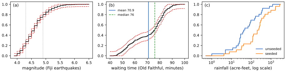
fig_7_s6. Download: PDF · SVGDemonstrations for this chapter
Each demonstration runs in the browser, on the book's data where possible, and links back to these notes. The ▶ Demo boxes above open them already set to the case under discussion.
| Demonstration | What you can see | Sections and results |
|---|---|---|
| The DKW band: one band for the whole cdf | The nerve data with the band at any level \(\alpha\) and intervals for \(F(b)-F(a)\); simulated samples from Normal, Cauchy, Exponential, Poisson(3) or the nerve data used as \(F\), with the simultaneous coverage of the band and of the pointwise intervals, and the exact coverage against \(n\). Presets: 1 Figure 7.1; 2 Exercise 7.3, Normal; 3 Exercise 7.3, Cauchy; 4 a discrete \(F\); 5 small \(n\). | 7.1; Theorem 7.5, Definition 7.A; Filling the gaps 7.4 to 7.6; Exercises 7.3, 7.6 |
| Plug-in estimators and their standard errors | Sampling distributions of six plug-in estimators against the Normal approximation \(N(T(F),\tau^2/n)\), the influence function, \(\hse\) and the coverage of (7.6), for five populations and three bivariate ones; a table of plug-in estimates for the nerve data. Presets: 1 the mean; 2 the variance; 3 the skewness; 4 the median; 5 the Old Faithful correlation. | 7.2; Theorem 7.9; Filling the gaps 7.7 to 7.12 |
| Glivenko–Cantelli: the largest gap goes to zero | \(D_n\) along up to 200 sample paths to \(n=10\,000\), with the DKW envelope, the typical size \(0.83/\sqrt n\) and the iterated-logarithm curve; the histogram of \(\sqrt nD_n\) against Kolmogorov's law. Presets: 1 one path; 2 100 paths; 3 Cauchy, distribution-free; 4 Poisson(3); 5 already Kolmogorov at \(n=10\). | Theorem 7.4, 7.5; Filling the gaps 7.3 to 7.5 |
Related demonstrations: the ECDF, DKW band and QQ-plot demo of Statistical Methods for Modern Biology (ECDFs of gene expression data), the Hoeffding interval demo of Chapter 4 (the one-point version of the DKW band), and the delta-method demo of Chapter 5. The Python code that produces every figure of this page is code/ch07_estimating_cdf.py (see the code index).
References
- Wasserman, L. (2004). All of Statistics: A Concise Course in Statistical Inference. Springer, New York. Chapter 7, pp. 97–105. www.stat.cmu.edu/~larry/all-of-statistics.
- Azzalini, A. and Bowman, A. W. (1990). A look at some data on the Old Faithful geyser. Applied Statistics, 39(3), 357–365.
- Cantelli, F. P. (1933). Sulla determinazione empirica delle leggi di probabilità. Giornale dell'Istituto Italiano degli Attuari, 4, 421–424.
- Chung, K. L. (1949). An estimate concerning the Kolmogoroff limit distribution. Transactions of the American Mathematical Society, 67, 36–50.
- Cox, D. R. and Lewis, P. A. W. (1966). The Statistical Analysis of Series of Events. Methuen, London.
- Donsker, M. D. (1952). Justification and extension of Doob's heuristic approach to the Kolmogorov–Smirnov theorems. The Annals of Mathematical Statistics, 23(2), 277–281.
- Dvoretzky, A., Kiefer, J. and Wolfowitz, J. (1956). Asymptotic minimax character of the sample distribution function and of the classical multinomial estimator. The Annals of Mathematical Statistics, 27(3), 642–669.
- Fisher, R. A. (1915). Frequency distribution of the values of the correlation coefficient in samples from an indefinitely large population. Biometrika, 10(4), 507–521.
- Glivenko, V. (1933). Sulla determinazione empirica delle leggi di probabilità. Giornale dell'Istituto Italiano degli Attuari, 4, 92–99.
- Hampel, F. R. (1974). The influence curve and its role in robust estimation. Journal of the American Statistical Association, 69(346), 383–393.
- Kolmogorov, A. N. (1933). Sulla determinazione empirica di una legge di distribuzione. Giornale dell'Istituto Italiano degli Attuari, 4, 83–91.
- Massart, P. (1990). The tight constant in the Dvoretzky–Kiefer–Wolfowitz inequality. The Annals of Probability, 18(3), 1269–1283.
- Scott, D. W., Gotto, A. M., Cole, J. S. and Gorry, G. A. (1978). Plasma lipids as collateral risk factors in coronary artery disease: a study of 371 males with chest pain. Journal of Chronic Diseases, 31, 337–345.
- Serfling, R. J. (1980). Approximation Theorems of Mathematical Statistics. Wiley, New York.
- Shorack, G. R. and Wellner, J. A. (1986). Empirical Processes with Applications to Statistics. Wiley, New York.
- Silverman, B. W. (1986). Density Estimation for Statistics and Data Analysis. Chapman and Hall, London.
- Simpson, J., Olsen, A. and Eden, J. C. (1975). A Bayesian analysis of a multiplicative treatment effect in weather modification. Technometrics, 17(2), 161–166.
- van der Vaart, A. W. (1998). Asymptotic Statistics. Cambridge University Press, Cambridge.
- van der Vaart, A. W. and Wellner, J. A. (1996). Weak Convergence and Empirical Processes. Springer, New York.
The numerical statements in the text (Example 7.2 and the nerve-data estimates, the exact and simulated coverage of the band, the elementary DKW bound, the Kolmogorov limits, the binomial law and covariance of \(\Fn\), the influence functions and their variances, the coverage of the Normal-based intervals, Example 7.15 and the solutions of the exercises) were confirmed numerically.